Stochastic second-order-cone complementarity problems

Math. Program., Ser. BDOI 10.1007/s10107-017-1121-z

FULL LENGTH PAPER

Stochastic second-order-cone complementarityproblems: expected residual minimization formulationand its applications

Gui-Hua Lin1 · Mei-Ju Luo2 · Dali Zhang3 ·Jin Zhang4

Received: 28 February 2015 / Accepted: 30 January 2017© Springer-Verlag Berlin Heidelberg and Mathematical Optimization Society 2017

Abstract This paper considers a class of stochastic second-order-cone complemen-tarity problems (SSOCCP), which are generalizations of the noticeable stochasticcomplementarity problems and can be regarded as the Karush–Kuhn–Tucker con-ditions of some stochastic second-order-cone programming problems. Due to theexistence of random variables, the SSOCCP may not have a common solution foralmost every realization . In this paper, motivated by the works on stochastic com-plementarity problems, we present a deterministic formulation called the expectedresidual minimization formulation for SSOCCP.We present an approximationmethodbased on the Monte Carlo approximation techniques and investigate some properties

This work was supported in part by NSFC (Nos. 11431004, 11501275, 71501127, 11671250, 11601458),Humanity and Social Science Foundation of Ministry of Education of China (No. 15YJA630034),Scientific Research Fund of Liaoning Provincial Education Department (No. L2015199), and Hong KongBaptist University FRG1/15-16/027.

B Gui-Hua [email protected]

Mei-Ju [email protected]

Dali [email protected]

Jin [email protected]

1 School of Management, Shanghai University, Shanghai 200444, China

2 School of Mathematics, Liaoning University, Shenyang 110036, Liaoning, China

3 Sino-US Global Logistics Institute, Antai College of Economics and Management, Shanghai JiaoTong University, Shanghai 200030, China

4 Department of Mathematics, Hong Kong Baptist University, Hong Kong, China

123

http://crossmark.crossref.org/dialog/?doi=10.1007/s10107-017-1121-z&domain=pdf

G.-H. Lin et al.

related to existence of solutions of the ERM formulation. Furthermore, we experi-ment some practical applications, which include a stochastic natural gas transmissionproblem and a stochastic optimal power flow problem in radial network.

Keywords SSOCCP · ERM formulation · Monte Carlo approximation · Natural gastransmission · Optimal power flow

Mathematics Subject Classification 90C15 · 90C30 · 90C33

1 Introduction

The second-order cone (SOC) in �ν is a closed cone defined as

Kν := {(x1, x2) ∈ � × �ν−1 | ‖x2‖ ≤ x1},

where ‖ · ‖ denotes the Euclidean norm. The second-order-cone complementarityproblem (SOCCP) is to find vectors x, y ∈ �n and z ∈ �l satisfying

x ∈ K, y ∈ K, xT y = 0, F(x, y, z) = 0, (1)

where F : �n × �n × �l → �n × �l is continuously differentiable and

K := Kn1 × · · · × Knm (2)

with n1 + · · · + nm = n. This problem is clearly a generalization of the classicalmixed complementarity problems and, especially, it includes the Karush–Kuhn–Tucker conditions of various second-order-cone programs (SOCP), which have lotsof applications in engineering design and portfolio optimization etc. [2], as specialcases. The SOCCP Eq. (1) has attracted much attention of many researchers and therehave been proposed several methods for solving it; see, e.g., [4,10,16,18].

In order to develop numerical algorithms for SOCCP, the so-called SOC comple-mentarity function φ : �ν × �ν → �ν satisfying

s ∈ Kν, t ∈ Kν, sT t = 0 ⇐⇒ φ(s, t) = 0 (3)

has been studied extensively. Two such functions known in the literature are presentedby Fukushima et al. in [16]: One is the vector-valued Fischer–Burmeister functionassociated with Kν defined as

φFB(s, t) := s + t − (s2 + t2)1/2 (4)

and the other is the natural residual function associated with Kν defined as

φNR(s, t) := s − [s − t]+, (5)

where [ · ]+ denotes the projection operator onto the convex cone Kν .

123

Stochastic second-order-cone complementarity problems…

To understand the above two functions, we need to review some basic concepts inJordan algebras. For any s = (s1, s2) ∈ � × �ν−1 and t = (t1, t2) ∈ � × �ν−1, theirJordan product is defined as

s ◦ t := (sT t, t1s2 + s1t2).

The identity element under this product is e := (1, 0, · · · , 0)T ∈ �ν and, forsimplicity, we denote by s2 = s ◦ s. See [13] for more details about the Jordan productassociated with symmetric cones.

We next recall the spectral factorization of vectors in �ν associated with the coneKν . It is well-known that any vector s = (s1, s2) ∈ � × �ν−1 can be decomposed as

s = λ1u1 + λ2u

2,

where {λ1, λ2} and {u1, u2} are respectively the spectral values and the associatedspectral vectors of s given by, for i = 1, 2,

λi := s1 + (−1)i ‖ s2 ‖,

ui :={

12

(1, (−1)i s2‖s2‖

)if s2 = 0,

12

(1, (−1)iw

)if s2 = 0

with w being an arbitrary unit vector in �ν−1. It is obvious that, if s2 = 0, the abovedecomposition is unique. It is shown in [16] that the projection of the vector s ontoKν can be written as

[s]+ = [λ1]+u1 + [λ2]+u2,

where [λ]+ := max{λ, 0} for a scalar λ ∈ �. Moreover, if s ∈ Kν , there exists aunique vector s1/2 ∈ Kν such that (s1/2)2 = s. Thus, the functions defined in Eqs. (4)and (5) can be represented as

φFB(s, t) = s + t − (s2 + t2)1/2 = s + t − (√

λ1u1 + √

λ2u2),

where {λ1, λ2} and {u1, u2} are given by, for i = 1, 2,

λi := ‖s‖2 + ‖t‖2 + 2(−1)i‖s1s2 + t1t2‖,

ui :={

12

(1, (−1)i s1s2+t1t2‖s1s2+t1t2‖

)if s1s2 + t1t2 = 0,

12

(1, (−1)iw

)if s1s2 + t1t2 = 0,

and

φNR(s, t) = s − [s − t]+ = s − ([λ1]+u1 + [λ2]+u2), (6)

123

G.-H. Lin et al.

where {λ1, λ2} and {u1, u2} are given by, for i = 1, 2,

λi := s1 − t1 + (−1)i‖s2 − t2‖, (7)

ui :={

12

(1, (−1)i s2−t2‖s2−t2‖

)if s2 = t2,

12

(1, (−1)iw

)if s2 = t2,

(8)

with w ∈ �ν−1 being an arbitrary unit vector. Note that both φFB and φNR are locallyLipschitz continuous but not differentiable everywhere [16].

Denote by x := (x1, · · · , xm) ∈ �n1 × · · · × �nm and y := (y1, · · · , ym) ∈�n1 ×· · ·×�nm . By means of the SOC complementarity function Eq. (3), the SOCCPEq. (1) can be easily reformulated as nonlinear equations

Φ(x, y) :=⎡⎢⎣

φ(x1, y1)...

φ(xm, ym)

⎤⎥⎦ = 0, F(x, y, z) = 0 (9)

and, along this approach, someNewton-typemethods have been developed for solvingEq. (1) successively. Another approach is to reformulate Eq. (1) as an optimizationproblem

min(x,y,z)

‖Φ(x, y)‖2 + ‖F(x, y, z)‖2

and some descent methods based on this approach are presented for solving Eq. (1).See [5] for more details about recent developments on SOCCP.

In this paper, we consider the following stochastic SOCCP (SSOCCP): Find vectorsx, y ∈ �n and z ∈ �l such that

x ∈ K, y ∈ K, xT y = 0, F(x, y, z, ξ) = 0 a.e. ξ ∈ Ω, (10)

where Ω denotes the support of the random variable ξ , F : �n × �n × �l × Ω →�n × �l , and a.e. is the abbreviation for “almost every”. This problem is obviously ageneralization of the stochastic complementarity problem (SCP)

x ≥ 0, F(x, ξ) ≥ 0, xTF(x, ξ) = 0 a.e. ξ ∈ Ω, (11)

which has been extensively studied in the recent literature. See [19] for more detailsabout the existing reformulations, numerical methods, and applications of Eq. (11).

Consider the stochastic optimization problem

min f (u)

s.t. h(u, ξ) = 0, g(u, ξ) ≤ 0 a.e. ξ ∈ Ω, (12)

where the objective may involve expectations or variances. This problem has manypractical applications such as water management in cooling-constrained power plants

123


[27], homogeneous product market [32], etc. Note that the problems with stochasticdominance constraints and the two-stage stochastic programs with recourse can berewritten in a generalized form of Eq. (12); see [12,26]. In addition, methodologiesfor some special cases of Eq. (12) are also considered; see, e.g., [28,32].

If some component functions of g(·, ξ) are SOC-representable [20], then Eq. (12)can be rewritten as a second-order-cone programming problem

min f (u)

s.t. h(u, ξ) = 0, H(x, u, ξ) = 0 a.e. ξ ∈ Ω,

x ∈ K. (13)

Recall that the SOC-representable functions include linear functions, convexquadratic functions, fractional quadratic functions, etc.; see, e.g., [2,20] for moredetails. Note that the equality constraints in Eq. (13) can be rewritten as

h(u) := Eξ [h(u, ξ) · h(u, ξ)] = 0,

H(x, u) := Eξ [H(x, u, ξ) · H(x, u, ξ)] = 0,

whereEξ denotes the expectation operator and · denotes the Hadamard product. Then,the Karush–Kuhn–Tucker system of problem Eq. (13) is

∇ f (u) + ∇ h(u)λ + ∇u H(x, u)μ = 0,

∇x H(x, u)μ − y = 0,

h(u, ξ) = 0, H(x, u, ξ) = 0 a.e. ξ ∈ Ω,

x ∈ K, y ∈ K, xT y = 0,

which is in the form of Eq. (10). This is one motivation to study the SSOCCP Eq. (10)in this paper. Besides, instead of rewriting Eq. (12) into Eq. (13) by the above SOC rep-resentable approach, our research is also inspired by some well-established practicalengineering SOC programming problems, as shown in Sects. 4.1 and 4.2. Specifically,engineers usually use the SOC convexification to attack malignant nonconvexity inpractice and it is interesting that the SOC relaxation may be exact with physicalexplanation in some cases (for instance, in Sect. 4.2, we study a circuit network oftree topology in which the alternating current optimal power flow (AC-OPF) admits anexact SOC relaxation). When uncertainty occurs (for example, the renewable resourceis involved; see Sect. 4.2), problem Eq. (13) appears naturally and motivates us toexplore the SSOCCP Eq. (10) as well.

However, because of the existence of the random element ξ , we generally cannotexpect that there exist vectors {x, y, z} satisfying Eq. (10) for almost every ξ ∈ Ω .This means that the SSOCCP Eq. (10) may not have a solution in general. Therefore,in order to get reasonable solutions in some senses, we need to present appropriatelydeterministic formulations for Eq. (10). In this paper, we mainly consider a deter-ministic formulation called expected residual minimization (ERM) formulation forEq. (10), which is motivated by the work [7] on the SCP Eq. (11). An approximation

123

G.-H. Lin et al.

method based on the Monte Carlo approximation techniques for solving the ERMmodel are proposed in Sect. 2 and some properties related to existence of solutionsof the ERM model are discussed in Sect. 3. Then, in Sect. 4, we report the modelingeffectiveness and computational efficiency of our investigations within the frameworkof two practical engineering settings, namely, a stochastic natural gas transmissionproblem and a stochastic optimal power flow problem in radial network.

Throughout this paper, we assume that the support set Ω is a compact set withinfinite number of elements in a finite dimensional Euclidean space and F(x, y, z, ξ) istwice continuously differentiable with respect to (x, y, z) and continuously integrablewith respect to ξ . For a given differentiable function H : �n → �m and a vectorx ∈ �n, ∇H(x) denotes the transposed Jacobian of H at x . Given a vector x ∈ �n

and a set X ⊆ �n , dist(x, X) denotes the distance from x to X under the Euclideannorm. For a given m × n matrix A = (ai j ), ‖A‖F denotes its Frobenius norm, thatis, ‖A‖F := (

∑mi=1

∑nj=1 a

2i j )

1/2. Moreover, I and O denote the identity matrix andnull matrix with suitable dimensions, respectively, and co{X} denotes the convex hullof a set X . In addition, we use sign(·) to stand for the sign function.

2 ERM formulation for SSOCCP

As introduced in Sect. 1, by means of the SOC complementarity function Eq. (3), theSSOCCP Eq. (10) can be reformulated as the stochastic nonlinear equations

Φ(x, y) = 0, F(x, y, z, ξ) = 0 a.e. ξ ∈ Ω,

where Φ is given as in Eq. (9). Recall that the above stochastic equations may nothave a common solution in general. Motivated by the work [7] on the SCP Eq. (11),we propose an ERM formulation for (10) as

min(x,y,z)

θERM(x, y, z) := Eξ [ ‖F(x, y, z, ξ)‖2 ] + ‖Φ(x, y)‖2. (14)

Onemain difficulty in dealingwithEq. (14) is that the problemcontains an expectation,which may have no analytical expression in general. We can employ the Monte Carlosampling techniques to approximate the expectation. Another possible difficulty is thatthe SOC complementarity function φ is generally not differentiable everywhere and sothe objective function may be nonsmooth. But this is not always the case. For the twoSOC complementarity functions introduced in Sect. 1, ‖φFB‖2 is actually a smoothfunction although φFB is nonsmooth, while ‖φNR‖2 and φNR are both nonsmoothfunctions.

As is known to us, the functions φFB and φNR are generalizations of the classicalreal-valued complementary functions

ϕFB(a, b) := a + b −√a2 + b2, (a, b) ∈ �2

123


and

ϕmin(a, b) := min{a, b}, (a, b) ∈ �2

respectively. Similarly to their prototypes, compared with each other, φFB owns bettersmoothing property and φNR has better approximation property. In particular, sinceφNR(s, t) = s − [s − t]+ = t − [t − s]+ for any s and t in �ν , we have

φNR(s, t) ={s if t − s ∈ Kν,

t if s − t ∈ Kν,

while there always exists a positive gap between φFB(s, t) and either s or t . Thisadvantage that φNR possesses may be particularly useful in dealing with the SOCCP

G(x) ∈ K, H(x) ∈ K, G(x)T H(x) = 0.

Our numerical experience reported in Sect. 4 also reveals that φNR may have betterperformance even though one fairly small smoothing parameter is involved. Furthercomparison between these two complementarity functions are given in Sect. 3.

In general, for an integrable function ψ : Ω → �, the Monte Carlo sam-pling estimate for Eξ [ψ(ξ)] is obtained by taking independently and identicallydistributed random samples Ωk := {ξ1, . . . , ξ Nk } from Ω and letting Eξ [ψ(ξ)] ≈1Nk

∑ξ i∈Ωk

ψ(ξ i ). We assume that Nk tends to infinity as k increases. The stronglaw of large numbers guarantees that this procedure converges with probability one(abbreviated by “w.p.1” below), that is,

limk→∞

1

Nk

∑ξ i∈Ωk

ψ(ξ i ) = Eξ [ψ(ξ)] w.p.1. (15)

In what follows, we consider two cases where φ is taken to be φFB and φNR inEq. (14) respectively.

2.1 The case of φFB

Consider the smooth ERM model

min(x,y,z)

θFB(x, y, z) := Eξ [ ‖F(x, y, z, ξ)‖2 ] + ‖ΦFB(x, y)‖2, (16)

whereΦFB denotes the functionΦ given in Eq. (9) by takingφ to beφFB. By generatingindependently and identically distributed random samples Ωk = {ξ1, . . . , ξ Nk } fromΩ , we can obtain the following approximation of Eq. (16):

min(x,y,z)

θkFB(x, y, z) := 1

Nk

∑ξ i∈Ωk

‖F(x, y, z, ξ i )‖2 + ‖ΦFB(x, y)‖2. (17)

123

G.-H. Lin et al.

We next study the convergence of the above sample average approximationmethod.Since (17) is a nonconvex optimization problem, we only investigate the limitingbehavior of its stationary points here. Actually, similar convergence result for its opti-mal solutions can be obtained more easily.

Theorem 1 Suppose that (xk, yk, zk) is a stationary point of problem Eq. (17) foreach k and (x, y, z) is an accumulation point of the sequence {(xk, yk, zk)}. Then(x, y, z) is a stationary point of problem Eq. (16) with probability one.

Proof Without loss of generality, we may assume limk→∞(xk, yk, zk) = (x, y, z).Let B be a compact and convex set containing the whole sequence {(xk, yk, zk)}. Bythe continuity of F , ∇(x,y,z)F, and ∇2

(x,y,z)Fj ( j = 1, . . . , n + l) on the compact set

B × Ω , there exists a constant C > 0 such that

‖F(x, y, z, ξ)‖ ≤ C, ‖∇(x,y,z)F(x, y, z, ξ)‖F ≤ C, (18)

‖∇2(x,y,z)Fj (x, y, z, ξ)‖F ≤ C ( j = 1, . . . , n + l) (19)

hold for every (x, y, z, ξ) ∈ B × Ω . Let

ΨFB(x, y) := ‖ΦFB(x, y)‖2.

By Proposition 2 of [6], ΨFB is smooth, that is, ∇ΨFB is continuous everywhere.For each k, since (xk, yk, zk) is stationary to problem Eq. (17), we have

2

Nk

∑ξ i∈Ωk

∇(x,y,z)F(xk, yk, zk, ξ i )F(xk, yk, zk, ξ i ) +[∇ΨFB(xk, yk)

0

]= 0. (20)

Consider the first term in the left–hand of Eq. (20). For each k and each j =1, . . . , n + l, we have

∣∣∣ 1

Nk

∑ξ i∈Ωk

∇(x,y,z)Fj (xk, yk, zk, ξ i )T F(xk, yk, zk, ξ i )

− 1

Nk

∑ξ i∈Ωk

∇(x,y,z)Fj (x, y, z, ξi )T F(x, y, z, ξ i )

∣∣∣≤ 1

Nk

∑ξ i∈Ωk

‖∇(x,y,z)Fj (xk, yk, zk, ξ i )‖ ‖F(xk, yk, zk, ξ i ) − F(x, y, z, ξ i )‖

+ 1

Nk

∑ξ i∈Ωk

‖∇(x,y,z)Fj (xk, yk, zk, ξ i )−∇(x,y,z)Fj (x, y, z, ξ

i )‖ ‖F(x, y, z, ξ i )‖

≤ C

Nk

∑ξ i∈Ωk

∫ 1

0

(‖∇(x,y,z)F(t xk+(1 − t)x, t yk+(1 − t)y, t zk+(1 − t)z, ξ i )‖F

+‖∇2(x,y,z)Fj (t x

k + (1 − t)x, t yk + (1 − t)y, t zk + (1 − t)z, ξ i )‖F)

123


×‖(xk, yk, zk) − (x, y, z)‖ dt≤ 2C2‖(xk, yk, zk) − (x, y, z)‖→ 0 as k → +∞,

where the second inequality follows from the mean-value theorem and Eq. (18), thethird inequality follows from Eqs. (18)–(19). We then have from Eq. (15) that

limk→∞

2

Nk

∑ξ i∈Ωk

∇(x,y,z)F(xk, yk, zk, ξ i )F(xk, yk, zk, ξ i )

= limk→∞

2

Nk

∑ξ i∈Ωk

∇(x,y,z)F(x, y, z, ξ i )F(x, y, z, ξ i )

= 2Eξ [ ∇(x,y,z)F(x, y, z, ξ)F(x, y, z, ξ) ]= Eξ [ ∇(x,y,z)(‖F(x, y, z, ξ)‖2) ]

holds with probability one. Moreover, by Eq. (18), we have

‖∇(x,y,z)F(x, y, z, ξ)F(x, y, z, ξ)‖ ≤ C2, (x, y, z, ξ) ∈ B × Ω

and hence, by Theorem 16.8 of [22],

limk→∞

2

Nk

∑ξ i∈Ωk

∇(x,y,z)F(xk, yk, zk, ξ i )F(xk, yk, zk, ξ i ) = ∇Eξ [ ‖F(x, y, z, ξ)‖2 ]

holds with probability one. Thus, letting k → +∞ in Eq. (20), we have

∇Eξ [ ‖F(x, y, z, ξ)‖2 ] + ∇ΨFB(x, y) = 0 w.p.1,

which means that (x, y, z) is a stationary point of Eq. (16) with probability one. ��

2.2 The case of φNR

Consider the nonsmooth ERM model

min(x,y,z)

θNR(x, y, z) := Eξ [ ‖F(x, y, z, ξ)‖2 ] + ‖ΦNR(x, y)‖2, (21)

whereΦNR denotes the functionΦ given in Eq. (9) by taking φ to be φNR. To deal withthis model, besides the Monte Carlo sampling techniques, some smoothing skills arealso necessary. Here, we employ the following smoothing approximation presented in[16] for the function φNR defined in Eq. (5): given a scalar μ > 0, let

φμNR(s, t) := s − 1

2

((

√λ21 + 4μ2 + λ1)u

1 + (

√λ22 + 4μ2 + λ2)u

2),

123

G.-H. Lin et al.

where {λ1, λ2} and {u1, u2} are the same as in Eqs. (7) and (8) respectively. It is shownin [16] that, for each (s, t) ∈ �2ν ,

limμ→+0

φμNR(s, t) = φNR(s, t)

and φμNR is a smooth function with

∇φμNR(s, t) =

[I − Mμ(s, t)Mμ(s, t)

], (22)

where

Mμ(s, t) :=

⎧⎪⎪⎪⎪⎪⎪⎪⎪⎪⎪⎨⎪⎪⎪⎪⎪⎪⎪⎪⎪⎪⎩

aμ(s, t)I if s2 − t2 = 0,

⎡⎢⎢⎣

bμ(s, t) dμ(s,t)(s2−t2)T

‖s2−t2‖

dμ(s,t)(s2−t2)‖s2−t2‖

(bμ(s,t)−cμ(s,t))(s2−t2)(s2−t2)T

‖s2−t2‖2 + cμ(s, t)I

⎤⎥⎥⎦

if s2 − t2 = 0

for s = (s1, s2) ∈ � × �ν−1 and t = (t1, t2) ∈ � × �ν−1 with

aμ(s, t) := s1−t12√

(s1−t1)2+4μ2+ 1

2 , (23)

bμ(s, t) := s1−t1−‖s2−t2‖4√

(s1−t1−‖s2−t2‖)2+4μ2+ s1−t1+‖s2−t2‖

4√

(s1−t1+‖s2−t2‖)2+4μ2+ 1

2 , (24)

cμ(s, t) := s1−t1√(s1−t1−‖s2−t2‖)2+4μ2+

√(s1−t1+‖s2−t2‖)2+4μ2

+ 12 , (25)

dμ(s, t) := − s1−t1−‖s2−t2‖4√

(s1−t1−‖s2−t2‖)2+4μ2+ s1−t1+‖s2−t2‖

4√

(s1−t1+‖s2−t2‖)2+4μ2. (26)

In addition, from the proof of Proposition 5.1 in [16], it is not difficult to see thatthere exists a positive constant C such that

‖φμNR(s, t) − φNR(s, t)‖ ≤ Cμ (27)

holds for each (s, t) ∈ �2ν .Taking a smoothing parameterμk > 0 and independently and identically distributed

random samples Ωk := {ξ1, . . . , ξ Nk } from Ω , we can obtain the following smoothapproximation of Eq. (21):

min(x,y,z)

θkNR(x, y, z) := 1

Nk

∑ξ i∈Ωk

‖F(x, y, z, ξ i )‖2 + ‖ΦμkNR(x, y)‖2, (28)

123


where

ΦμNR(x, y) :=

⎡⎢⎣

φμNR(x1, y1)

...

φμNR(xm, ym)

⎤⎥⎦

for x = (x1, . . . , xm) ∈ �n1 × . . . × �nm and y = (y1, . . . , ym) ∈ �n1 × · · · × �nm .Suppose that μk → +0 as k → +∞. We next study the convergence of the abovesample average approximation method. As mentioned in the last subsection, we onlyneed to investigate the limiting behavior of stationary points of problem Eq. (28)because similar convergence result for optimal solutions can be obtained more easily.To this end, the following definitions are useful.

Definition 1 [11] Let H : �p → �q be locally Lipschitz continuous. The Clarkegeneralized gradient of H at w is defined as

∂H(w) := co{

limw′→w,w′∈DH

∇H(w′)},

where DH denotes the set of points at which H is differentiable.

Definition 2 [18] Let H : �p → �q be locally Lipschitz continuous and Hμ :�p → �q be a function such that Hμ is continuously differentiable everywhere forany μ > 0 and limμ→+0 Hμ(w) = H(w) for any w ∈ �p. We say that Hμ satisfiesthe Jacobian consistency with H if

limμ→+0

dist(∇Hμ(w), ∂H(w)

) = 0

holds for any w ∈ �p.

For simplicity, we denote by

ΨNR(x, y) := ‖ΦNR(x, y)‖2, ΨμNR(x, y) := ‖Φμ

NR(x, y)‖2,and, for x = (x1, . . . , xm) ∈ �n1×· · ·×�nm and y = (y1, . . . , ym) ∈ �n1×· · ·×�nm ,we let

Ψ iNR(xi , yi ) := ‖φNR(xi , yi )‖2, Ψ

μ,iNR (xi , yi ) := ‖φμ

NR(xi , yi )‖2

for each i . Then we have

∂ΨNR(x, y) = ∂Ψ 1NR(x1, y1) × · · · × ∂Ψ m

NR(xm, ym) (29)

and

∇ΨμNR(x, y) =

⎡⎢⎣

∇Ψμ,1NR (x1, y1)

...

∇Ψμ,mNR (xm, ym)

⎤⎥⎦ . (30)

123

G.-H. Lin et al.

By Theorem 4.9 of [18], we have the following lemma immediately.

Lemma 1 The function ΨμNR satisfies the Jacobian consistency with ΨNR.

We next show the main convergence result of this subsection.

Theorem 2 Suppose that (xk, yk, zk) is a stationary point of problem Eq. (28) foreach k and (x, y, z) is an accumulation point of the sequence {(xk, yk, zk)}. Then(x, y, z) is a stationary point of problem Eq. (21) with probability one.

Proof Without loss of generality,wemay assume limk→∞(xk, yk, zk) = (x, y, z). LetB and C > 0 be the same as in the proof of Theorem 1. For each k, since (xk, yk, zk)is stationary to problem Eq. (28), we have

2

Nk

∑ξ i∈Ωk

∇(x,y,z)F(xk, yk, zk, ξ i )F(xk, yk, zk, ξ i ) +[∇Ψ

μkNR(xk, yk)

0

]= 0.(31)

In a similar way to the proof of Theorem 1, we can show that

limk→∞

2

Nk

∑ξ i∈Ωk

∇(x,y,z)F(xk, yk, zk, ξ i )F(xk, yk, zk, ξ i )

= ∇Eξ [ ‖F(x, y, z, ξ)‖2 ] (32)

holds with probability one. We next show

limk→∞ dist

(∇ΨμkNR(xk, yk), ∂ΨNR(x, y)

) = 0.

Denote by xk := (xk,1, . . . , xk,m) ∈ �n1 × · · · × �nm , yk := (yk,1, . . . , yk,m) ∈�n1 × · · · × �nm for each k and by x := (x1, . . . , xm) ∈ �n1 × · · · × �nm , y :=(y1, . . . , ym) ∈ �n1 × · · · × �nm . From Eqs.( 29) and ( 30), it is sufficient to showthat, for each i ,

limk→∞ dist

(∇Ψμk ,iNR (xk,i , yk,i ), ∂Ψ i

NR(x i , yi )) = 0. (33)

First of all, for any given i , we have

∥∥φμkNR(xk,i , yk,i ) − φ

μkNR(x i , yi )

∥∥≤ ∥∥φ

μkNR(xk,i , yk,i ) − φNR(xk,i , yk,i )

∥∥ + ∥∥φNR(xk,i , yk,i ) − φNR(x i , yi )∥∥

+∥∥φNR(x i , yi ) − φμkNR(x i , yi )

∥∥≤ 2Cμk + ∥∥φNR(xk,i , yk,i ) − φNR(x i , yi )

∥∥→ 0 as k → +∞, (34)

where the second inequality follows from Eq. (27). We consider five cases:

123


(I) Suppose that x i = yi . It follows that λ j = x i1 − yi1 + (−1) j‖x i2 − yi2‖ = 0 forj = 1, 2. By Theorem 4.6 and Proposition 4.8 of [18], we have

∂Ψ iNR(x i , yi ) =

{2

[I − VV

]φNR(x i , yi )

∣∣∣∣ V ∈ co(O, I, S)

},

where

S :={1

2

[1 wT

w (1 + β)I − βwwT

] ∣∣∣∣ β ∈ [−1, 1], ‖w‖ = 1

}.

It is not difficult to see from Eqs. (23)–(26) that any accumulation points of thesequences

{aμk (xk,i , yk,i )}, {bμk (x

k,i , yk,i )}, {cμk (xk,i , yk,i )}, {dμk (x

k,i , yk,i )}

belong to the intervals [0, 1], [0, 1], [0, 1], [0, 12 ] respectively. Therefore, any

accumulation point of {Mμk (xk,i , yk,i )}must belong to co(O, I, S). On the other

hand, it is easy to see from Eqs. (27) and (34) that limk→∞ φμkNR(xk,i , yk,i ) =

φNR(x i , yi ). Therefore, by Eq. (22), we can obtain Eq. (33) easily.(II) Suppose that x i = yi and x i2 − yi2 = 0. Since {∇φ

μkNR(xk,i , yk,i )} is bounded, we

have from Eq. (34) that

limk→∞ ∇φ

μkNR(xk,i , yk,i )

(φ

μkNR(xk,i , yk,i ) − φ

μkNR(x i , yi )

) = 0. (35)

On the other hand, it is easy to see from Eqs. (23)–(26) that

limk→∞ aμk (x

k,i , yk,i ) = limk→∞ bμk (x

k,i , yk,i ) = limk→∞ cμk (x

k,i , yk,i )

= 1

2sign(x i1 − yi1) + 1

2

and limk→∞ dμk (xk,i , yk,i ) = 0, which means

limk→∞

(Mμk (x

k,i , yk,i ) − Mμk (xi , yi )

) = 0 (36)

and hence

limk→∞

(∇φμkNR(xk,i , yk,i ) − ∇φ

μkNR(x i , yi )

) = 0. (37)

Since {φμkNR(x i , yi )} is bounded, we have

limk→∞

(∇φμkNR(xk,i , yk,i ) − ∇φ

μkNR(x i , yi )

)φ

μkNR(x i , yi ) = 0. (38)

123

G.-H. Lin et al.

Therefore, it follows from Eqs. (35) and (38) that

1

2

∥∥∇Ψμk ,iNR (xk,i , yk,i ) − ∇Ψ

μk ,iNR (x i , yi )

∥∥= ∥∥∇φ

μkNR(xk,i , yk,i )φμk

NR(xk,i , yk,i ) − ∇φμkNR(x i , yi )φμk

NR(x i , yi )∥∥

≤ ∥∥∇φμkNR(xk,i , yk,i )

(φ

μkNR(xk,i , yk,i ) − φ

μkNR(x i , yi )

)∥∥+∥∥(∇φ

μkNR(xk,i , yk,i ) − ∇φ

μkNR(x i , yi )

)φ

μkNR(x i , yi )

∥∥→ 0 as k → +∞.

By Lemma 1, we have

limk→∞ dist

(∇Ψμk ,iNR (x i , yi ), ∂Ψ i

NR(x i , yi )) = 0

and hence Eq. (33) holds.(III) Suppose that x i2 − yi2 = 0 and |x i1 − yi1| = ‖x i2 − yi2‖. From Eqs. (23)–(26), we

have

limk→∞

(aμk (x

k,i , yk,i ) − aμk (xi , yi )

) = limk→∞

(bμk (x

k,i , yk,i ) − bμk (xi , yi )

) = 0,

limk→∞

(cμk (x

k,i , yk,i ) − cμk (xi , yi )

) = limk→∞

(dμk (x

k,i , yk,i ) − dμk (xi , yi )

) = 0,

which implies Eq. (36) and hence Eq. (37). In a similar way to (II), we can getEq. (33).

(IV) Suppose that x i2 − yi2 = 0 and x i1 − yi1 = ‖x i2 − yi2‖. It follows that λ1 = 0 andλ2 > 0. By Theorem 4.6 and Proposition 4.8 of [18], we have


{2

[I − VV

]φNR(x i , yi )

∣∣∣∣ V ∈ co(I, I + Z)

},

where

Z := 1

2

⎡⎢⎣ −1

(x i2−yi2)T

‖x i2−yi2‖x i2−yi2

‖x i2−yi2‖− (x i2−yi2)(x

i2−yi2)

T

‖x i2−yi2‖2

⎤⎥⎦ .

Note that, by Eqs. (23)–(26), any accumulation points of the sequences

{bμk (xk,i , yk,i )}, {cμk (x

k,i , yk,i )}, {dμk (xk,i , yk,i )}

belong to [ 12 , 1], [ 12 , 1], [0, 12 ] respectively. It is not difficult to see that any

accumulation point of {Mμk (xk,i , yk,i )} must belong to co(I, I + Z). Since

limk→∞ φμkNR(xk,i , yk,i ) = φNR(x i , yi ), by Eq. (22), we can obtain Eq. (33)

easily.

123


(V) Suppose that x i2 − yi2 = 0 and x i1 − yi1 = −‖x i2 − yi2‖. It follows that λ1 < 0 andλ2 = 0. By Theorem 4.6 and Proposition 4.8 of [18], we have


{2

[I − VV

]φNR(x i , yi )

∣∣∣∣ V ∈ co(O, Z)

},

where

Z := 1

2

⎡⎢⎣ 1

(x i2−yi2)T

‖x i2−yi2‖x i2−yi2

‖x i2−yi2‖(x i2−yi2)(x

i2−yi2)

T

‖x i2−yi2‖2

⎤⎥⎦ .

In a similar way to (IV), we can show Eq. (33).

As a result, Eq. (33) holds in all cases. Letting k → +∞ in Eq. (31), we have fromEqs. (32)–(33) that

0 ∈ ∇Eξ [ ‖F(x, y, z, ξ)‖2 ] + ∂ΨNR(x, y) × {0} w.p.1,

which means that (x, y, z) is a stationary point of Eq. (21) with probability one. ��

2.3 Exponential convergence rate

In this subsection, we show that, with the increase of sample size, the optimal solutionsof the approximation problem Eqs. (17) or (28) converge exponentially to a solutionof the ERM formulation Eqs. (16) or (21) with probability approaching one undersuitable conditions. To this end, we first introduce a lemma.

Lemma 2 [28]LetW be a compact set and h : W×Ω → � be integrable everywhere.Suppose that the following conditions hold:

(i) For every w ∈ W, the moment generating function

Eξ

[et (h(w,ξ)−Eξ [h(w,ξ)])]

is finite-valued for all t in a neighbourhood of zero.(ii) There exist a measurable function κ : Ω → �+ and a constant γ > 0 such that

|h(w′, ξ) − h(w, ξ)| ≤ κ(ξ)‖w′ − w‖γ

for all ξ ∈ Ω and all w′, w ∈ W.(iii) The moment generating function Eξ [etκ(ξ)] is finite-valued for all t in a neigh-

bourhood of zero.

123

G.-H. Lin et al.

Then, for every ε > 0, there exist positive constants D(ε) and β(ε), independentof Nk, such that

Prob{supw∈W

∣∣∣ 1

Nk

∑ξ i∈Ωk

h(w, ξ i ) − Eξ [h(w, ξ)]∣∣∣ ≥ ε

}≤ D(ε)e−Nkβ(ε).

Applying the above lemma, we can obtain the following result related to the expo-nential convergence of the above approximation methods.

Theorem 3 Let (xk, yk, zk) be an optimal solution of Eq. (17) or Eq.( 28) for each kand (x, y, z) be an accumulation point of the sequence {(xk, yk, zk)}. Then, for everyε > 0, there exist positive constants D(ε) and β(ε), independent of Nk, such that

Prob{|θkFB(xk, yk, zk) − θFB(x, y, z)| ≥ ε

}≤ D(ε)e−Nkβ(ε) (39)

or

Prob{|θkNR(xk, yk, zk) − θNR(x, y, z)| ≥ ε

}≤ D(ε)e−Nkβ(ε). (40)

Proof Without loss of generality, we assume that {(xk, yk, zk)} itself converges to(x, y, z). Let B be a compact set that contains the whole sequence {(xk, yk, zk)}.

(1) Consider the case for Eq. (17). We first show that there exist positive constantsD(ε) and β(ε) such that

Prob{

sup(x,y,z)∈B

|θkFB(x, y, z) − θFB(x, y, z)| ≥ ε}

≤ D(ε)e−Nkβ(ε), (41)

which is equivalent to show

Prob{

sup(x,y,z)∈B

∣∣∣ 1

Nk

∑ξ i∈Ωk

‖F(x, y, z, ξ i )‖2 − Eξ [‖F(x, y, z, ξ)‖2]∣∣∣ ≥ ε

}

≤ D(ε)e−Nkβ(ε)

by Eqs. (16) and (17). To do this, it is sufficient to prove that the set W := B and thefunction h(x, y, z, ξ) := ‖F(x, y, z, ξ)‖2 satisfy the conditions given in Lemma 2. Infact, since both Ω and B are compact, by the continuous differentiability assumptionon F given in Sect. 1, these conditions hold.

Since (xk, yk, zk) is an optimal solution of Eq. (17) for each k, in a similar wayto Theorem 1, we can show that (x, y, z) is an optimal solution of Eq. (14). It thenfollows that

θkFB(xk, yk, zk) ≤ θkFB(x, y, z), θFB(x, y, z) ≤ θFB(xk, yk, zk),

123


from which we have

θkFB(xk, yk, zk) − θFB(x, y, z)

= θkFB(xk, yk, zk) − θkFB(x, y, z) + θkFB(x, y, z) − θFB(x, y, z)

≤ θkFB(x, y, z) − θFB(x, y, z)

≤ sup(x,y,z)∈B

|θkFB(x, y, z) − θFB(x, y, z)|

and

θkFB(xk, yk, zk) − θFB(x, y, z)

= θkFB(xk, yk, zk) − θFB(xk, yk, zk) + θFB(xk, yk, zk) − θFB(x, y, z)

≥ θkFB(xk, yk, zk) − θFB(xk, yk, zk)

≥ − sup(x,y,z)∈B

|θkFB(x, y, z) − θFB(x, y, z)|.

It follows that

|θkFB(xk, yk, zk) − θFB(x, y, z)| ≤ sup(x,y,z)∈B

|θkFB(x, y, z) − θFB(x, y, z)|.

This together with Eq. (41) implies Eq. (39).(2) Consider the case for Eq. 28. In this case, it is sufficient to show that the setW :=

B×[0, μ0] and the function h(x, y, z, μ, ξ) := ‖F(x, y, z, ξ)‖2 +ΦμNR(x, y) satisfy

the conditions given in Lemma 2. In fact, this can be guaranteed by the assumptionsgiven at the end of Sect. 1 and Eq. (27). Thus, in a similar manner to (1), we can showEq. (40) easily. This completes the proof. ��

2.4 Boundedness of level sets

It iswell known that the boundedness of the iteration sequences is a desired requirementfor various optimization methods. In order to ensure the boundedness of the iterationsequence, we generally investigate the boundedness of level sets. Given a nonnegativenumber γ , the level set of the ERM model Eq. 14 is given as

LERM(γ ) := {(x, y, z) ∈ �2n+l | θERM(x, y, z) ≤ γ }.

Note that, if there is some ni > 1 and we take

xk := (· · · , k, k, 0, · · · , 0︸︷︷︸Kni

, · · · )T , yk := (· · · , k,−k, 0, · · · , 0︸︷︷︸Kni

, · · · )T

for every k, then both xk and yk belong to the cone K and they are perpendicular toeach other. This means Φ(xk, yk) = 0 for each k, where Φ is given in Eq. 9 with φ

123

G.-H. Lin et al.

to be an SOC complementarity function, regardless of whether it takes φFB or φNR.As a result, we can only investigate the conditions on the mapping F to guarantee theboundedness of the level set LERM(γ ).

Definition 3 [30] The mapping H : �p × Ω → �q is locally coercive if, for any{wk} ⊆ �p satisfying ‖wk‖ → +∞, we have

Prob{ limk→∞ ‖H(wk, ξ)‖ = +∞} > 0.

The main result of this subsection can be stated as follows.

Theorem 4 Suppose that F is locally coercive. Then, for any γ ≥ 0, the level setLERM(γ ) is bounded.

Proof Suppose on the contrary that there exist a constant γ > 0 and a sequence{(xk, yk, zk)} ⊆ �2n+l with ‖(xk, yk, zk)‖ → +∞ such that

θERM(xk, yk, zk) ≤ γ

for each k. It follows that

γ ≥ Eξ [ ‖F(xk, yk, zk, ξ)‖2 ] ≥ (Eξ [ ‖F(xk, yk, zk, ξ)‖ ])2 (42)

for each k. By the Fatou’s lemma [22], we have

Eξ [ lim infk→∞ ‖F(xk, yk, zk, ξ)‖ ] ≤ lim inf

k→∞ Eξ [ ‖F(xk, yk, zk, ξ)‖ ]. (43)

Note that F is locally coercive, which means that

Prob{ limk→∞ ‖F(xk, yk, zk, ξ)‖ = +∞} > 0.

Therefore, the left-hand side in Eq. (43) is infinity and hence

lim infk→∞ Eξ [ ‖F(xk, yk, zk, ξ)‖ ] = +∞,

which contradicts Eq. (42) and so the level set LERM(γ ) is bounded for any γ ≥ 0. ��

3 Comparison between φNR and φFB

As stated at the beginning of Sect. 2, the function φFB generally owns better smoothingproperty, while the function φNR has better approximation property. On the otherhand, Chen and Fukushima [7] show that, in the one-dimensional case, φNR has someproperty that φFB does not possess; see Lemma 2.2 and Example 1 given in [7] fordetails. An interesting and natural question is whether the result can be extended tomulti-dimensional cases. We devote to answer this question in this section.

123


Consider the following special affine SSOCCP:

x ∈ K, M(ξ)x + q(ξ) ∈ K, xT (M(ξ)x + q(ξ)) = 0 a.e. ξ ∈ Ω, (44)

where M : Ω → �n×n and q : Ω → �n . For Eq. (44), it is natural to suggest itsERM formulation as follows:

minx

θ(x) := Eξ [ ‖Φ(x, M(ξ)x + q(ξ))‖2 ], (45)

where Φ is the same as in Eq. (9). Then we have the following result for φNR.

Theorem 5 Let Ω := {ξ1, ξ2, . . . , ξ N } and each ni ≤ 2 in Eq.( 2). Then the solutionset of problem Eq. (45) with φ to be φNR is nonempty.

Proof First of all, we show that ‖φNR(s, t)‖2 is a piecewise quadratic function overpolyhedral partitions in (s, t) ∈ �ni × �ni when ni ≤ 2. In fact, it is evident thatφNR(s, t) = min{s, t} is piecewise quadratic when ni = 1. Next, we suppose ni = 2and consider the following five cases:

(I) Suppose that s2 − t2 = 0. It is easy to see that

‖φNR(s, t)‖2 ={ ‖s‖2 if s1 ≤ t1, s2 = t2,

‖t‖2 if s1 ≥ t1, s2 = t2.

(II) Suppose that s1 − t1 ≥ |s2 − t2| > 0. This means s − t ∈ K2 and hence

‖φNR(s, t)‖2 = ‖t‖2

from the discussion at the beginning of Sect. 2.(III) Suppose that s1 − t1 ≤ −|s2 − t2| < 0. This means t − s ∈ K2 and, similarly to

(II), we have

‖φNR(s, t)‖2 = ‖s‖2.

(IV) Suppose that s2 − t2 > 0 and t2 − s2 ≤ s1 − t1 ≤ s2 − t2. By Eqs. (6)–(8), wehave

‖φNR(s, t)‖2 =∥∥∥s − [s1 − t1 − |s2 − t2|]+( 12 ,− s2−t2

2|s2−t2| )T

−[s1 − t1 + |s2 − t2|]+( 12 ,s2−t2

2|s2−t2| )T∥∥∥2

= 1

4(s1 + t1 − s2 + t2)

2 + 1

4(−s1 + t1 + s2 + t2)

2.

(V) Suppose that s2 − t2 < 0 and s2 − t2 ≤ s1 − t1 ≤ t2 − s2. By Eqs. (6)–(8), wehave

123

G.-H. Lin et al.

‖φNR(s, t)‖2 =∥∥∥s − [s1 − t1 − |s2 − t2|]+( 12 ,− s2−t2

2|s2−t2| )T

−[s1 − t1 + |s2 − t2|]+( 12 ,s2−t2

2|s2−t2| )T∥∥∥2

= 1

4(s1 + t1 + s2 − t2)

2 + 1

4(s1 − t1 + s2 + t2)

2.

In summary, from the continuity of the function φNR, we have

‖φNR(s, t)‖2 =

⎧⎪⎪⎪⎪⎨⎪⎪⎪⎪⎩

t21 + t22 if s1 − t1 ≥ s2 − t2, s1 − t1 ≥ t2 − s2,s21 + s22 if t1 − s1 ≥ s2 − t2, t1 − s1 ≥ t2 − s2,14 (s1 + t1 − s2 + t2)2 + 1

4 (−s1 + t1 + s2 + t2)2

if t2 − s2 ≤ s1 − t1 ≤ s2 − t2, s2 − t2 ≥ 0,14 (s1 + t1 + s2 − t2)2 + 1

4 (s1 − t1 + s2 + t2)2 otherwise,

which indicates that ‖φNR(s, t)‖2 is indeed a piecewise quadratic function over poly-hedral partitions in (s, t).

Note that the objective function of Eq. (45) can be written as

θ(x) =m∑i=1

N∑j=1

p j ‖φNR(xi , yij )‖2,

where x := (x1, . . . , xm) ∈ �n1 × · · · × �nm , M(ξ j )x + q(ξ j ) := (y1j , . . . , ymj ) ∈

�n1 ×· · ·×�nm for each j = 1, . . . , N , and p j denotes the probability of the sampleξ j for each j = 1, . . . , N . From the above discussion, it is not difficult to see that theobjective function θ is piecewise quadratic function over polyhedral partitions. Sincethis function is bounded below on whole space, by the Frank–Wolfe theorem given in[15], problem Eq. (45) has an optimal solution at least. This completes the proof. ��

Theorem 5 indicates that Lemma 2.2 in [7] can be extended from one-dimensionalcases to two-dimensional cases. It is still an open question whether the lemma canbe extended to general cases. Note that, by Example 1 given in [7], the conclusion inTheorem 5 does not hold for the case of φFB.

Remark 1 If we rewrite the affine SSOCCP Eq. (44) by introducing an additionalvariable as the form

x ∈ K, y ∈ K, xT y = 0, y − M(ξ)x + q(ξ) = 0 a.e. ξ ∈ Ω

and consider its ERM model

min(x,y)

Eξ [ ‖y − M(ξ)x − q(ξ)‖2 ] + ‖Φ(x, y)‖2 (46)

instead of problem Eq. (45), then we can get an interesting and understandable result,that is, Theorem 5 remains true without the discrete assumption related to the sample

123


space Ω (we can show this result in a very similar way and so omit its proof here).Our next question is how about the case of φFB? Note that Example 1 in [7] can notserve as a counterexample in this case. In fact, for this example, the model Eq. (46)becomes

min(x,y)

y2 + 1 + (x + y −√x2 + y2)2,

which attains its infimum at x∗ = 0 and y∗ = 0 obviously. We are not sure whetherthe model Eq. (46) with φ to be φFB has similar conclusion as φNR. We would like toleave it as a future work.

4 Applications

The theoretical results given in the previous sections indicate that the SSOCCPEq. (10)can be solved via the variation schemeEq. (14). In this section, as a further supplement,we consider two practical engineering problems.

4.1 Natural gas production and transportation

Natural gas is one of the fastest-growing energy sources. How to plan the generationand distribution of natural gas in transmission networks is becoming a key issue ingas production and transportation. Recently, a substantial number of studies focus onnatural gas transmission optimization problems [23,25,29]. The most difficult issuein optimization is from the nonlinear relationship between the transmission flow in apipeline and the pressures at two ends of the pipeline, and the uncertainty of losses atcompressor stations. In this subsection, we implement the ERM framework to solvethis type of problems.

Consider an optimizationmodel for a natural gas network1 consisted by a number ofhub-and-spoke subnetworks where every hub is a compressor station with a number offields andmarkets connected to and only to it.Wedenote byN := {1, 2, . . . , N } the setof nodes in the transmission network, which is classified into three subsets: Ng ⊂ Nof all field nodes with producers, Ns ⊂ N of all station nodes with compressors bywhich every gas flow is split into two or more pipelines, and Nm ⊂ N of all marketnodes with consumptions. Without loss of generality, we assume that the intersectionsbetween any two of the above subsets are empty. This assumption can be achievedby introducing virtual pipelines. For every node i ∈ N , we have two sets of nodesconnected to it: I(i), the set of nodes with pipelines going into node i , and O(i), theset of nodes with pipelines going out node i . It is worth emphasizing that, due to thehub-and-spoke structure, for any i ∈ Ng , I(i) is empty and O(i) is a singleton withits element being the station node to which node i is connected. Similarly, for anyi ∈ Nm , O(i) is empty and I(i) is a singleton with its element being the station nodefrom which node i is connected.

1 We refer readers to [3,25] for detailed analysis on how to model natural gas production and transmission.

123

G.-H. Lin et al.

Uncertainties often occur in transmission operations (for example, a small propor-tion of the gas flow at a station is tapped off transmission pipelines to provide fuel forthe compressors at the station; see, e.g., Sect. V in [31]). Here, we take the losses atstations as uncertainties and denote by ξi the loss at node i ∈ Ns . We also denote thelosses at all compressor stations by a random vector ξ := (ξ1, . . . , ξS), where S is thenumber of stations in the network.

The transmission network is centrally operated to deliver natural gas for each mar-ket.Wedenote by p j (Q j ) the unit price of natural gas inmarket j ∈ Nm ,where p j (Q j )

is a decreasing function with respect to the supply quantity Q j into market j . In ourstudy, we consider an extensively investigated price function p j (Q j ) := a j −b jQ j forevery j ∈ Nm . At field nodes, before real transmissions, the producers are contractedfor their minimum generations. We use Gi to denote the minimum generation at nodei and Ci to denote the unit generation cost of natural gas at field i ∈ Ng .

Now we introduce the parameters for pipelines. We denote by Pmaxi j and Pmin

i j

(Pmaxi j and Pmin

i j ) the maximum and minimum pressures at the inlet (outlet) end of

the pipeline from node i to node j for i, j ∈ N . Here, we define Pmaxi j = Pmin

i j = 0

and Pmaxi j = Pmin

i j = 0 when i and j are not connected. To generate one unit inletpressure for the pipeline from i to j , a cost ci j is incurred. In our model, the pressuresat the inlet ends of the pipelines connecting from fields to stations are fixed by theproduction contract and denoted by Pi j for every i ∈ Ng and the corresponding stationnode j ∈ O(i), which is enforced by the production standards. On the other hand, thepressures at the inlet ends of the pipelines connecting tomarkets from stations are fixedby the supply contracts and denoted by Pji for every i ∈ Nm and the correspondingstation node j ∈ I(i), which is predetermined based on the market standards.

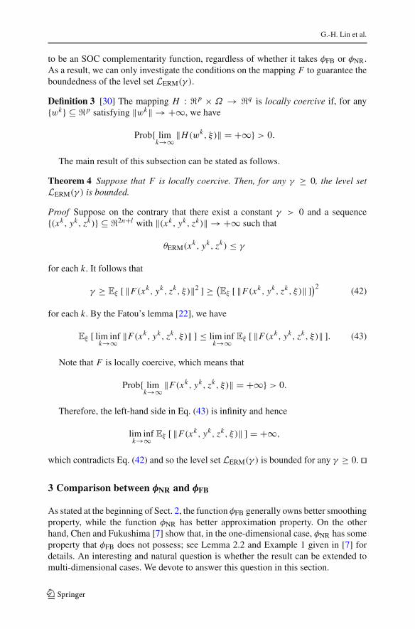
The nonlinear relationship between the pressure difference at two ends of a pipelineand the quantity of natural gas transmitted through this pipeline can be described viathe Weymouth equation. In particular, the flow qi j for the pipeline connecting nodesi and j is upper bounded by

qci j (pi j , pi j ) := Ki j

√(pi j )2 − (pi j )2, (47)

where pi j and pi j are the inlet and outlet pressures, respectively, and Ki j is a constantcomputed from the physical properties of this pipeline such as length, dimension,friction factor, etc.2

2 For a particular pipeline, the Weymouth equation can be expressed as (see (1) and (2) in [1] with theadjustment on parameter units)

qci j (pi j , pi j ) = 77.52 × 10−6 ×(Tbpb

)D5/2

√(pi j )2−(pi j )2

γg ZT L f ,

where Tb is the base temperature (unit R), pb is the base pressure (unit psia), D is the inside diameter (unitin), γg is the gas specific gravity (air = 1), Z is the gas deviation factor at average flowing temperature andaverage pressure, T is the average flowing temperature (unit R), L is the length of pipe (unit mile), and fis the Moody friction factor.

123


020

4060

80

020

4060

800

20

40

60

80

100

120

ˆijpij

qij

020

4060

80

020

4060

800

20

40

60

80

100

120

ˆij

pij

qij

(a) (b)

p p

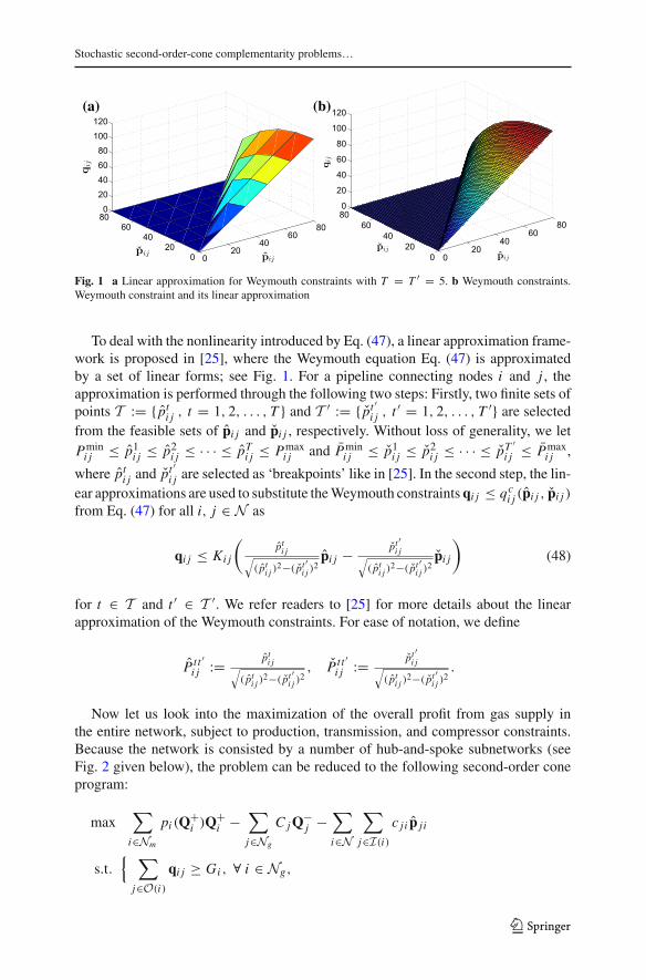
Fig. 1 a Linear approximation for Weymouth constraints with T = T ′ = 5. b Weymouth constraints.Weymouth constraint and its linear approximation

To deal with the nonlinearity introduced by Eq. (47), a linear approximation frame-work is proposed in [25], where the Weymouth equation Eq. (47) is approximatedby a set of linear forms; see Fig. 1. For a pipeline connecting nodes i and j , theapproximation is performed through the following two steps: Firstly, two finite sets ofpoints T := { pti j , t = 1, 2, . . . , T } and T ′ := { pt ′i j , t ′ = 1, 2, . . . , T ′} are selectedfrom the feasible sets of pi j and pi j , respectively. Without loss of generality, we letPmini j ≤ p1i j ≤ p2i j ≤ · · · ≤ pTi j ≤ Pmax

i j and Pmini j ≤ p1i j ≤ p2i j ≤ · · · ≤ pT

′i j ≤ Pmax

i j ,

where pti j and pt′i j are selected as ‘breakpoints’ like in [25]. In the second step, the lin-

ear approximations are used to substitute theWeymouth constraintsqi j ≤ qci j (pi j , pi j )from Eq. (47) for all i, j ∈ N as

qi j ≤ Ki j

(pti j√

( pti j )2−( pt

′i j )

2pi j − pt

′i j√

( pti j )2−( pt

′i j )

2pi j

)(48)

for t ∈ T and t ′ ∈ T ′. We refer readers to [25] for more details about the linearapproximation of the Weymouth constraints. For ease of notation, we define

P tt ′i j := pti j√

( pti j )2−( pt

′i j )

2, P tt ′

i j := pt′i j√

( pti j )2−( pt

′i j )

2.

Now let us look into the maximization of the overall profit from gas supply inthe entire network, subject to production, transmission, and compressor constraints.Because the network is consisted by a number of hub-and-spoke subnetworks (seeFig. 2 given below), the problem can be reduced to the following second-order coneprogram:

max∑i∈Nm

pi (Q+i )Q+

i −∑j∈Ng

C jQ−j −

∑i∈N

∑j∈I(i)

c ji p j i

s.t.{ ∑

j∈O(i)

qi j ≥ Gi , ∀ i ∈ Ng,

123

G.-H. Lin et al.

q2i j + K 2i j p

2i j ≤ K 2

i j p2i j , ∀ i ∈ Ng, j ∈ O(i),

q2j i + K 2j i p

2j i ≤ K 2

j i p2j i , ∀ i ∈ Nm, j ∈ I(i),

qi j ≤ Ki j

(P tt ′i j pi j − P tt ′

i j pi j)

, ∀ t ∈ T , t ′ ∈ T ′, i ∈ Ns, j ∈ O(i) ∩ Ns,

Q+i =

∑j∈I(i)

q j i , ∀ i ∈ N ,

Q−i =

∑j∈O(i)

qi j , ∀ i ∈ N ,

Q−i − Q+

i ≤ −ξi , ∀ i ∈ Ns,

Pmini j ≤ pi j ≤ Pmax

i j , ∀ j ∈ N , i ∈ I( j),

Pmini j ≤ pi j ≤ Pmax

i j , ∀ j ∈ N , i ∈ I( j)}

∀ ξi , i ∈ Ns . (49)

Here, the decision variables include the vectors of inlet pressures, outlet pressures,and flow quantities transmitted in the pipelines and are denoted respectively by

⎧⎨⎩p := (

p12, . . . , p1N , . . . , pi j , . . . , pN1, . . . , pN (N−1)),

p := (p12, . . . , p1N , . . . , pi j , . . . , pN1, . . . , pN (N−1)

),

q := (q12, . . . ,q1N , . . . ,qi j , . . . ,qN1, . . . ,qN (N−1)

),

the intermediate variables Q+i and Q−

i are the total quantities transmitted into andout node i respectively for each i ∈ N . The objective function includes three terms:the total revenue with pi (Q

+i )Q+

i to be the revenue obtained from market i ∈ Nm ,the production costs in the fields with Q−

i to be the quantity of gas produced in fieldi ∈ Ng , and the operation costs spent for generating pressures. It is straightforwad tosee that the objective function is concave and quadratic.

Now let us go through the constraints. The first set of constraints is on the pro-ductions of natural gas at field nodes, which means that the gas quantity transmittedout a field must be no less than the minimum contracted production. The second setof constraints is on the flow quantities transmitted in a pipeline from field nodes. Bysetting Pmax

i j = 0 for any unconnected pair i ∈ Ng and j ∈ N , we have pi j = 0 andhence qi j = pi j = 0. The third set of constraints is on the flow quantities transmittedin a pipeline to market nodes. By setting Pmax

j i = 0 for any unconnected pair i ∈ Nm

and j ∈ N , we have p j i = 0 and hence q j i = p j i = 0.

Remark 2 Note that the second set of constraints in Eq. (49) can be rewritten as

√q2i j + K 2

i j p2i j ≤ Ki j pi j

for every i ∈ Ng and the corresponding j ∈ O(i). Similarly, the third set of constraintsin Eq. (49) can be rewritten as

√q2j i + K 2

j i p2j i ≤ K ji p j i

123


for every i ∈ Nm and the corresponding j ∈ I(i). Therefore, these two sets ofconstraints are actually SOC constraints.

The fourth set of constraints is on the flow in a pipeline connecting two stationnodes, where the linear approximations are implemented to reformulate the constraintsqi j ≤ qci j (pi j , pi j ), i = j and i, j ∈ Ns , into linear constraints, where qci j (pi j , pi j ) isgiven as in Eq. (47).

Remark 3 In [25], this typeof linear approximations has beenused for every pipeline ina transmission network, where the number of constraints resulted from linear approx-imation is N (N − 1) × T × T ′. For the network with hub-and-spoke substructure,the second, third and fourth sets of constraints show that we only need to implementthe linear approximations to the pipelines connecting stations and so the number ofconstraints on pipeline flows can be reduced in our problem.

The fifth and sixth sets of constraints define Q+i and Q−

i as the quantities of flowstransmitted into and out node i ∈ N . The seventh set of constraints is on the randomlosses at station nodes, where ξi is the quantity of the natural gas tapped off at stationi ∈ Ns . The eighth and ninth sets of constraints are from the upper and lower boundsof inlet pressures and outlet pressures of pipelines. Recall that Pmax

i j = Pmini j = 0 and

Pmaxi j = Pmin

i j = 0 when i and j are not connected. Recall also that the pressures atinlet ends of pipelines connecting from fields are fixed by the contracts and thus wedefine Pmax

i j = Pmini j = Pi j for all i ∈ Ng and, similarly, the inlet ends of pipelines

connecting to the markets from stations are fixed by the supply contracts and thus wedefine Pmax

j i = Pminj i = Pji for all i ∈ Nm .

It is worth mentioning that, in the real world, the natural gases produced at differentfields are usuallywith different percentages of their chemical components, where thesepercentages are often used tomeasure the quality of natural gases.Accordingly, anotherset of constraints has to be made on inlet and outlet pressures to control the mixed gasat each station to achieve the contracted quality standard.

To concentrate our focus on applying theoretical framework, we assume that thenatural gas qualities at different fields are the same and never changed in the transmis-sion. This assumption can be relaxed by introducing a set of linear equality constraintsfor mass balance on each component; see, e.g., [25].

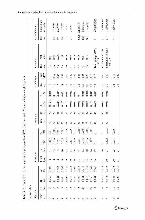
Before proceeding to the numerical tests, we summarize the notation on parametersused in the model in Table 1.

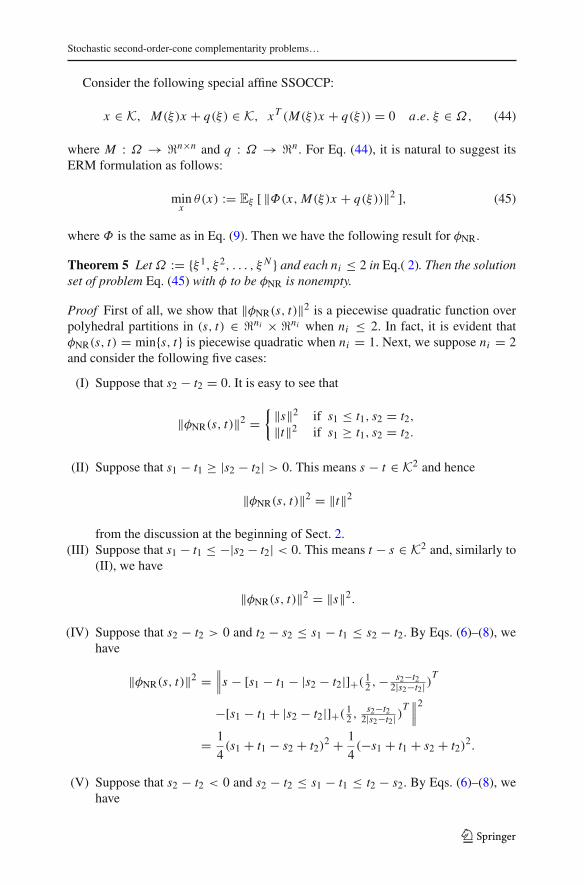
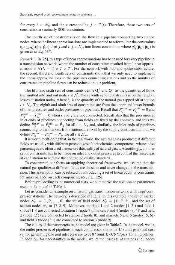
Let us consider an example on a natural gas transmission network with three com-pressor stations. The network is described in Fig. 2. In this example, the set of marketnodes Nm = {1, 2, . . . , 6}, the set of field nodes Ng = {1′, 2′, 3′}, and the set ofstation nodes Ns = {7, 8, 9}. Moreover, markets 1 and 2 (nodes {1, 2}) and field 1(node {1′}) are connected to station 1 (node 7), markets 3 and 4 (nodes {3, 4}) and field2 (node {2′}) are connected to station 2 (node 8), and markets 5 and 6 (nodes {5, 6})and field 3 (node {3′}) are connected to station 3 (node 9).

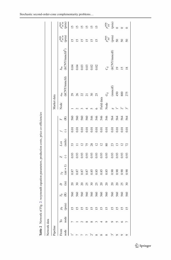
The values of the parameters in the model are given in Table 2. In the model, we fixthe outlet pressures of pipelines to each compressor station at 15 (unit: psia) and costci j for generating one unit inlet pressure to be 87 (unit: k×CNY/psia) for all pipelines.In addition, for uncertainties in the model, we let the losses ξi at stations (i.e., nodes

123

G.-H. Lin et al.

Table 1 Notation

Gi Minimum production at field i ∈ Ng

Ki j Weymouth constant for pipeline from node i to j ∈ O(i)

P t t ′i j , P t t ′

i j Coefficients in the linear approximation of Weymouth equations

Pmini j , Pmax

i j Lower and upper bounds on inlet end of pipeline from i to j ∈ O(i)

Pmini j , Pmax

i j Lower and upper bounds on outlet end of pipeline from i to j ∈ O(i)

ai − biQ+i Unit price for gas in market i ∈ Nm

Ci unit cost for gas production in field i ∈ Ng

ci j Unit cost for generating pressure at an end of pipeline from i ∈ Nto j ∈ O(i)

Fig. 2 Structure of the natural gas network

i = 7, 8, 9) follow normal distribution with means being 15, 20, 10 and variancesbeing 5.5, 9.0, 3.5, respectively.

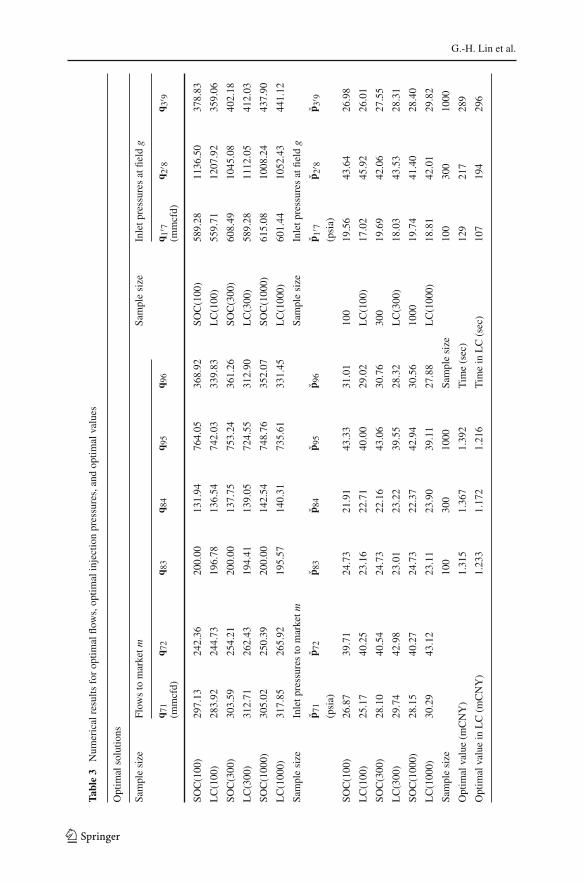
In our numerical tests, we used the linear approximation Eq. (48) with T = T ′ =10 for the Weymouth equation Eq. (47). Note that the linear approximation doesnot change the objective function and other constraints. We solved our optimizationproblems and the problems in [25] with the same samples of ξ . In Table 3, we denoteour optimization problem and the problem in [25] by SOC(n) and LC(n) respectively,where n is the sample size in each test. In our tests, we varied n from 100, 300 to 1000and compared the results of SOC(n) and LC(n).

We implemented the ERM scheme to solve this model and analyzed the impactof loss uncertainties at stations to the overall profit and optimal operations in thetransmission network. The results given in Table 3 were obtained by using the functionφNR. The problems were solved in the GAMS platform byNLP solver. Table 3 lists the

123


Table2

Networkof

Fig.

2:weymouth

equatio

nparameters,productio

ncosts,priceco-efficiencies

Networkdata

Pipelin

eMarketd

ata

From

Top b

T bD

γg

ZLen

fT

Nod

ea m

b mpm

inm

′ mpm

axm

′ mno

deno

de(psia)

(R)

(in)

(air=1)

(-)

(mile

)(-)

(R)

(kCNY/m

mcfd)

(kCNY/m

mcfd2)

(psia)

(psia)

1′7

1556

020

0.87

0.93

330.01

560

129

0.04

1515

71

1556

030

0.87

0.93

110.01

560

226

0.04

1515

72

1556

020

0.87

0.93

120.01

560

322

0.03

1515

78

1556

025

0.87

0.93

750.01

560

421

0.03

1515

2′8

1556

030

0.85

0.93

280.01

546

530

0.02

1515

83

1556

025

0.85

0.93

120.01

546

625

0.02

1515

84

1556

020

0.85

0.93

120.01

546

Fielddata

89

1556

020

0.85

0.93

800.01

546

Nod

eGg

Cg

pmax

gg′

pmin

gg′

3′9

1556

020

0.90

0.93

230.01

564

g(m

mcdf)

(kCNY/m

mcdf)

(psia)

(psia)

95

1556

020

0.90

0.93

130.01

564

1′45

019

500

96

1556

025

0.90

0.93

120.01

564

2′80

015

500

97

1556

030

0.90

0.93

720.01

564

3′27

518

500

123

G.-H. Lin et al.

Table3

Num

ericalresults

foroptim

alflo

ws,optim

alinjectionpressures,andoptim

alvalues

Optim

alsolutio

ns

Samplesize

Flow

sto

marketm

Samplesize

Inletp

ressures

atfield

g

q 71

q 72

q 83

q 84

q 95

q 96

q 1′ 7

q 2′ 8

q 3′ 9

(mmcfd)

(mmcfd)

SOC(100

)29

7.13

242.36

200.00

131.94

764.05

368.92

SOC(100

)58

9.28

1136

.50

378.83

LC(100

)28

3.92

244.73

196.78

136.54

742.03

339.83

LC(100

)55

9.71

1207

.92

359.06

SOC(300

)30

3.59

254.21

200.00

137.75

753.24

361.26

SOC(300

)60

8.49

1045

.08

402.18

LC(300

)31

2.71

262.43

194.41

139.05

724.55

312.90

LC(300

)58

9.28

1112

.05

412.03

SOC(100

0)30

5.02

250.39

200.00

142.54

748.76

352.07

SOC(100

0)61

5.08

1008

.24

437.90

LC(100

0)31

7.85

265.92

195.57

140.31

735.61

331.45

LC(100

0)60

1.44

1052

.43

441.12

Samplesize

Inletp

ressures

tomarketm

Samplesize

Inletp

ressures

atfield

g

p 71

p 72

p 83

p 84

p 95

p 96

p 1′ 7

p 2′ 8

p 3′ 9

(psia)

(psia)

SOC(100

)26

.87

39.71

24.73

21.91

43.33

31.01

100

19.56

43.64

26.98

LC(100

)25

.17

40.25

23.16

22.71

40.00

29.02

LC(100

)17

.02

45.92

26.01

SOC(300

)28

.10

40.54

24.73

22.16

43.06

30.76

300

19.69

42.06

27.55

LC(300

)29

.74

42.98

23.01

23.22

39.55

28.32

LC(300

)18

.03

43.53

28.31

SOC(100

0)28

.15

40.27

24.73

22.37

42.94

30.56

1000

19.74

41.40

28.40

LC(100

0)30

.29

43.12

23.11

23.90

39.11

27.88

LC(100

0)18

.81

42.01

29.82

Samplesize

100

300

1000

Samplesize

100

300

1000

Optim

alvalue(m

CNY)

1.31

51.36

71.39

2Tim

e(sec)

129

217

289

Optim

alvaluein

LC(m

CNY)

1.23

31.17

21.21

6Tim

ein

LC(sec)

107

194

296

123


sample averaged solutions. Here, to avoid redundancy, we only report the main resultsin approximation solutions for inlet pressures in pipelines, gas quantities transmittedby pipelines, and the optimal values of objective function under different sample sizes.

Notice that, in our method, the linear approximation is only incorporated for theconstraints of gas quantities in pipelines connecting stations rather than all pipelines in‘LC(n)’. Therefore, we can take the results solved from the ‘LC(n)’ model as approx-imation to the results in ‘SOC(n)’. From another point of view, both models can betaken as approximations to the true natural gas transmission problem, where ‘SOC(n)’is closer with less number of linear approximation of the Weymouth constraints. Forcomputational time, the results show that solving the model with second-order coneconstraint is almost at the same level as ‘LC(n)’ with a little longer computationaltime.

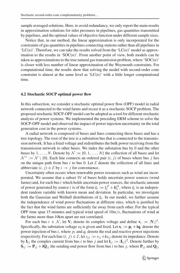
4.2 Stochastic SOCP optimal power flow

In this subsection, we consider a stochastic optimal power flow (OPF) model in radialnetwork connected to the wind farms and recast it as a stochastic SOCP problem. Theproposed stochastic SOCP-OPFmodel can be adopted as a tool for different stochasticanalysis of power systems. We implemented the preceding ERM scheme to solve theSOCP-OPF model and observed the impact of power injection uncertainty on the totalgeneration cost in the power systems.

A radial network is composed of buses and lines connecting these buses and has atree topology. The root of the tree is a substation bus that is connected to the transmis-sion network. It has a fixed voltage and redistributes the bulk power receiving from thetransmission network to other buses. We index the substation bus by 0 and the otherbuses by 1, . . . , N . Denote by N := {0, 1, . . . , N } the collection of all buses and letN+ := N \ {0}. Each line connects an ordered pair (i, j) of buses where bus j lieson the unique path from bus i to bus 0. Let E denote the collection of all lines andabbreviate (i, j) ∈ E by i → j for convenience.

Uncertainty often occurs when renewable power resources such as wind are incor-porated. We assume that a subset W of buses holds uncertain power sources (windfarms) and, for each bus i which holds uncertain power sources, the stochastic amountof power generated by source i is of the form ξi := ξ

pi + iξqi , where ξi is an indepen-

dent random variable with known mean and deviation. In particular, we investigateboth the Gaussian and Weibull distributions of ξi . In our model, we further assumethe independence of wind power fluctuations at different sites, which is justified bythe fact that the wind farms are sufficiently far away from each other. For the typicalOPF time span 15 minutes and typical wind speed of 10m/s, fluctuations of wind atthe farms more than 10km apart are not correlated.

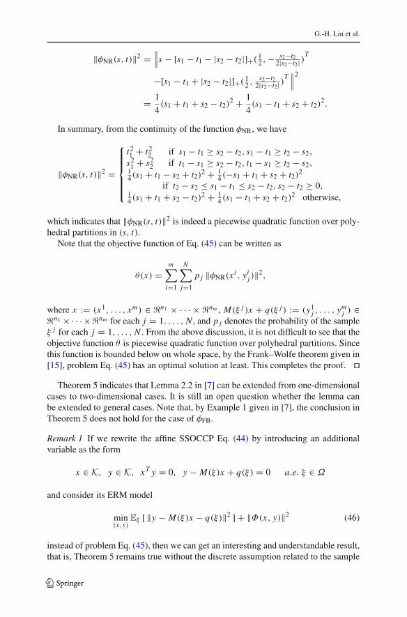
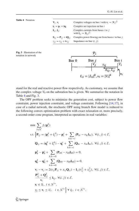
For each bus i ∈ N , let Vi denote its complex voltage and define vi := |Vi |2.Specifically, the substation voltage v0 is given and fixed. Let si := pi + iqi denote thepower injection of bus i , where pi and qi denote the real and reactive power injectionsrespectively. For each line (i, j) ∈ E , let zi j := ri j +ixi j denote its impedance. Denoteby Ii j the complex current from bus i to bus j and let li j := |Ii j |2. Denote further bySi j := Pi j + iQi j the sending-end power flow from bus i to bus j , where Pi j and Qi j

123

G.-H. Lin et al.

Table 4 NotationVi , vi Complex voltages on bus i with vi = |Vi |2si = pi + iqi Complex net injection on bus i

Ii j , li j Complex currents from buses i to jwith li j = |Ii j |2

Si j = Pi j + iQi j Complex power flowing out from buses i to bus j

zi j = ri j + ixi j Impedance on line (i, j)

Fig. 3 Illustration of thenotation in network

stand for the real and reactive power flow respectively. As customary, we assume thatthe complex voltage V0 on the substation bus is given. We summarize the notation inTable 4 and Fig. 3.

The OPF problem seeks to minimize the generation cost, subject to power flowconstraint, power injection constraint, and voltage constraint. Following [14,17], incase of a radial network, the stochastic OPF using branch flow model is reduced tothe following convex optimization problem with exact relaxation or, more precisely,a second-order cone program, interpreted as operations in real variables:

min∑i∈N

fi (pgi )

s·t·{Pi j = (pgi + ξ

pi ) − pci +

∑h:h→i

(Phi − rhi lhi ), ∀(i, j) ∈ E,

Qi j = (qgi + ξqi ) − qci +

∑h:h→i

(Qhi − xhi lhi ), ∀(i, j) ∈ E,

pg0 − pc0 +∑

h:h→0

(Ph0 − rh0lh0) = 0,

qg0 − qc0 +∑

h:h→0

(Qh0 − xh0lh0) = 0,

vi − v j = 2(ri jPi j + xi jQi j ) − li j (r2i j + x2i j ), ∀(i, j) ∈ E,

P2i j + Q2

i j

vi≤ li j , ∀(i, j) ∈ E,

si ∈ Si , i ∈ N+,

vi ≤ vi ≤ vi , i ∈ N+} ∀ ξi , i ∈ N+,

123


where ξi := ξpi + iξqi , pi := pci − pgi and qi := qci − qgi are the real and reactive net

loads at node i . In particular, pci and qci are the real and reactive power consumptionat node i , pgi and qgi are the real and reactive conventional power generation at nodei . We use h : h → i to denote a collection of buses inN prior to i in the tree networktopology with (h, i) ∈ E and use h : h → 0 to denote the collection of buses in Nprior to the substation root with (h, 0) ∈ E . In addition, we assume that each fi isconvex quadratic and, particularly, fi (p

gi ) := ci2(p

gi )

2 + ci1pgi + ci0 in our model.

Notice that the convex relaxed power flow equation li j ≥ P2i j+Q2

i jvi

, (i, j) ∈ E , isexactly in the form of a rotated second-order cone in �4, which is a convex set givenas

K2r := {(x1, x2, x3) ∈ � × � × �2 | x1x2 ≥ xT3 x3, x1 ≥ 0, x2 ≥ 0}.

Trivially, the rotated second-order cone in �4 can be expressed as a linear transfor-mation (actually, a rotation) of the (plain) second-order cone in �4, due to

x1x2 ≥ xT3 x3, x1 ≥ 0, x2 ≥ 0 ⇐⇒∥∥∥∥[x1 − x22x3

] ∥∥∥∥ ≤ x1 + x2.

Recall that (x1, x2, x3) ∈ K2r if and only if (x1 + x2, x4) ∈ K4, where x4 :=

(x1−x2, 2x3). For a clear presentation in the subsequent discussion,we recast the abovedistribution network stochastic dispatch problem in the following compact SOCPform:

min f (x)

s·t·{x ∈ X ,

Ax + Bξ = 0,

‖Gix‖ ≤ gTi x, ∀ i with (i, j) ∈ E}

∀ ξ, (50)

where the vector x represents all dispatching variables related to optimal power flowof the distribution network, f (x) represents the total generation cost, and X is thefeasible set of radial distribution network.

Notice that Eq. (50) actually coincides with the linear form of Eq. (13), which is notcomputationally trackable by any commonly-used commercial SOCP solvers such asMOSEK or Gurobi. Our key step toward numerical solution of problem Eq. (50) is toreformulate it into the SSOCCP Eq. (10) by its KKT system, as discussed previously.Hence, as in convex programming, the KKT conditions are necessary and sufficientfor global optimality [21]. As each KKT point is a global minimizer of Eq. (50), wemay consider to solve Eq. (50) by searching its KKT points, which is exactly what wehave discussed in the preceding sections for SSOCCP.

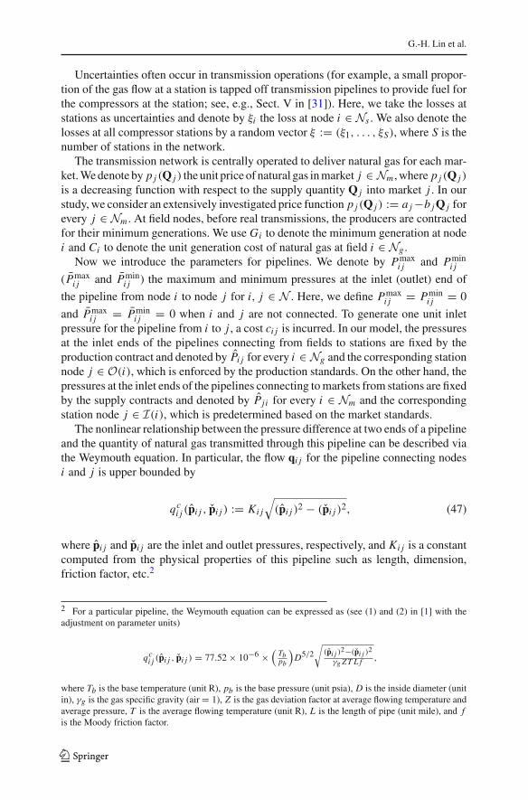
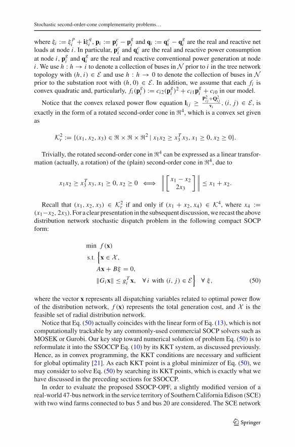
In order to evaluate the proposed SSOCP-OPF, a slightly modified version of areal-world 47-bus network in the service territory of Southern California Edison (SCE)with two wind farms connected to bus 5 and bus 20 are considered. The SCE network

123

G.-H. Lin et al.

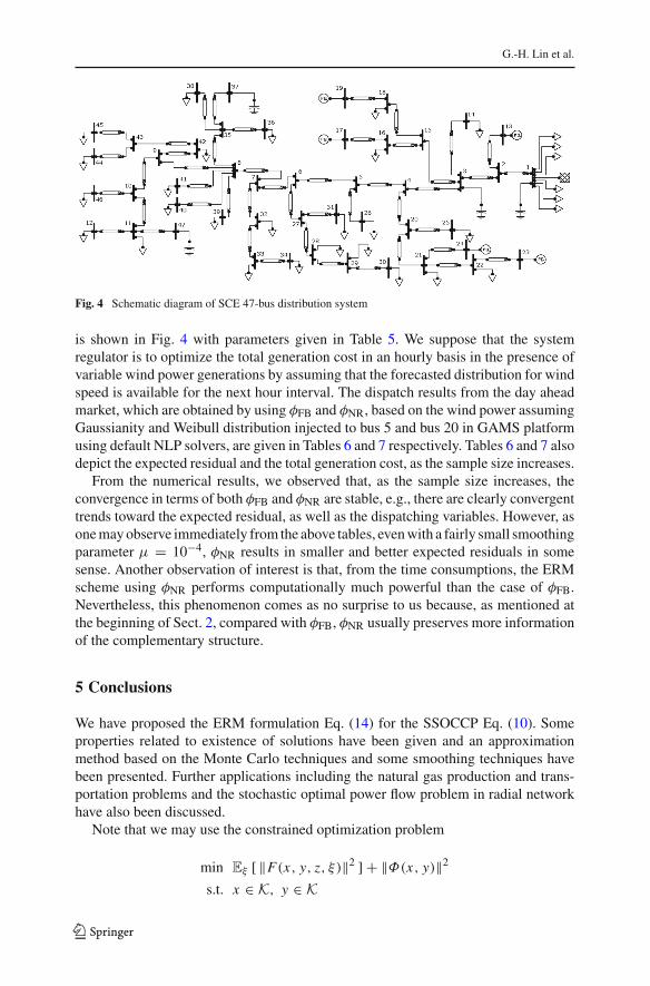
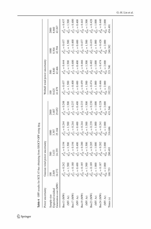
Fig. 4 Schematic diagram of SCE 47-bus distribution system

is shown in Fig. 4 with parameters given in Table 5. We suppose that the systemregulator is to optimize the total generation cost in an hourly basis in the presence ofvariable wind power generations by assuming that the forecasted distribution for windspeed is available for the next hour interval. The dispatch results from the day aheadmarket, which are obtained by using φFB and φNR, based on the wind power assumingGaussianity and Weibull distribution injected to bus 5 and bus 20 in GAMS platformusing default NLP solvers, are given in Tables 6 and 7 respectively. Tables 6 and 7 alsodepict the expected residual and the total generation cost, as the sample size increases.

From the numerical results, we observed that, as the sample size increases, theconvergence in terms of both φFB and φNR are stable, e.g., there are clearly convergenttrends toward the expected residual, as well as the dispatching variables. However, asonemayobserve immediately from the above tables, evenwith a fairly small smoothingparameter μ = 10−4, φNR results in smaller and better expected residuals in somesense. Another observation of interest is that, from the time consumptions, the ERMscheme using φNR performs computationally much powerful than the case of φFB.Nevertheless, this phenomenon comes as no surprise to us because, as mentioned atthe beginning of Sect. 2, compared with φFB, φNR usually preserves more informationof the complementary structure.

5 Conclusions

We have proposed the ERM formulation Eq. (14) for the SSOCCP Eq. (10). Someproperties related to existence of solutions have been given and an approximationmethod based on the Monte Carlo techniques and some smoothing techniques havebeen presented. Further applications including the natural gas production and trans-portation problems and the stochastic optimal power flow problem in radial networkhave also been discussed.

Note that we may use the constrained optimization problem

min Eξ [ ‖F(x, y, z, ξ)‖2 ] + ‖Φ(x, y)‖2s.t. x ∈ K, y ∈ K

123


Table5

Networkof

Fig.

1:lin

eim

pedances,p

eakspot

load

KVA,capacito

rsandPV

generatio

n’snameplateratin

gs

Networkdata

Linedata

Linedata

Linedata

Loaddata

Loaddata

PVgenerators

From

ToR

XFrom

ToR

XFrom

ToR

XBus

Peak

Bus

Peak

Bus

Nam

eplate

bus

bus

(Ω)

(Ω)

bus

bus

(Ω)

(Ω)

bus

bus

(Ω)

(Ω)

no.

MVA

no.

MVA

no.

capacity

12

0.25

90.80

88

410.10

70.03

121

220.19

80.04

61

1034

0.2

213

00

835

0.07

60.01

522

230

011

0.67

360.27

131.5MW

23

0.03

10.09

28

90.03

10.03

127

310.04

60.01

512

0.45

380.45

170.4MW

34

0.46

0.09

29

100.01

50.01

527

280.10

70.03

114

0.89

391.34

191.5MW

314

0.09

20.03

19

420.15

30.04

628

290.10

70.03

116

0.07

400.13

231MW

315

0.21

40.04

610

110.10

70.07

629

300.06

10.01

518

0.67

410.67

242MW

420

0.33

60.06

110

460.22

90.12

232

330.04

60.01

521

0.45

420.13

45

0.10

70.18

311

470.03

10.01

533

340.03

10

222.23

440.45

Shun

tcapacito

rs

526

0.06

10.01

511

120.07

60.04

635

360.07

60.01

525

0.45

450.2

Bus

Nam

plate

56

0.01

50.03

115

180.04

60.01

535

370.07

60.04

626

0.2

460.45

No.

1capacity

627

0.16

80.06

115

160.10

70.01

535

380.10

70.01

528

0.13

67

0.03

10.04

616

170

042

430.06

10.01

529

0.13

Basevolta

ge(K

V)

=12

.35

16000

KVAR

732

0.07

60.01

518

190

043

440.06

10.01

530

0.2

BaseKVA=10

003

1200

KVAR

78

0.01

50.01

520

210.12

20.09

243

450.06

10.01

531

0.07

Substatio

nvolta

ge=12

.35

3718

00KVAR

840

0.04

60.01

520

250.21

40.04

632

0.13

4718

00KVAR

839

0.22

40.04

621

240

033

0.27

123

G.-H. Lin et al.

Table6

OPF

results

forSC

E47-bus

obtainingfrom

SSOCP-OPF

using

φFB

Power

uncertainty

Gausian

windpower

uncertainty

Weibullwindpower

uncertainty

Samplesize

100

500

1000

2000

100

500

1000

2000

Exp

ectedresidu

al2.84

93.43

33.39

73.40

78.62

58.84

08.50

48.66

0Generationcost(M

W)

24.272

24.255

25.104

25.052

41.879

42.466

42.594

42.267

Bus13

(MW)

pg 13=

0.24

2pg 13

=0.19

4pg 13

=0.24

4pg 13

=0.24

8pg 13

=0.43

7pg 13

=0.44

4pg 13

=0.43

7pg 13

=0.43

7

(MVAr)

qg 13

=1.50

0qg 13

=1.50

0qg 13

=1.50

0qg 13

=1.50

0qg 13

=1.50

0qg 13

=1.50

0qg 13

=1.50

0qg 13

=1.50

0

Bus17

(MW)

pg 17=

0.18

0pg 17

=0.19

4pg 17

=0.24

4pg 17

=0.23

7pg 17

=0.40

0pg 17

=0.40

0pg 17

=0.40

0pg 17

=0.40

0

(MVAr)

qg 17

=0.40

0qg 17

=0.40

0qg 17

=0.40

0qg 17

=0.40

0qg 17

=0.40

0qg 17

=0.40

0qg 17

=0.40

0qg 17

=0.40

0

Bus19

(MW)

pg 19=

0.18

5pg 19

=0.20

0pg 19

=0.24

4pg 19

=0.23

3pg 19

=0.45

9pg 19

=0.46

6pg 19

=0.43

7pg 19

=0.44

3

(MVAr)

qg 19

=1.50

0qg 19

=1.50

0qg 19

=1.50

0qg 19

=1.50

0qg 19

=1.50

0qg 19

=1.50

0qg 19

=1.50

0qg 19

=1.50

0

Bus23

(MW)

pg 23=

0.18

9pg 23

=0.20

5pg 23

=0.23

9pg 23

=0.23

0pg 23

=0.47

4pg 23

=0.48

2pg 23

=0.41

9pg 23

=0.42

8

(MVAr)

qg 23

=1.00

0qg 23

=1.00

0qg 23

=1.00

0qg 23

=1.00

0qg 23

=1.00

0qg 23

=1.00

0qg 23

=1.00

0qg 23

=1.00

0

Bus24

(MW)

pg 24=

0.18

7pg 24

=0.20

2pg 24

=0.24

1pg 24

=0.22

8pg 24

=0.46

6pg 24

=0.47

4pg 24

=0.42

8pg 24

=0.44

0

(MVAr)

qg 24

=2.00

0qg 24

=2.00

0qg 24

=2.00

0qg 24

=2.00

0qg 24

=2.00

0qg 24

=2.00

0qg 24

=2.00

0qg 24

=2.00

0

Tim

es(s)

168.75

328

0.49

331

6.68

643

1.54

619

2.22

132

1.74

024

0.38

245

4.49

1

123


Table7

OPF

results

forSC

E47-bus

obtainingfrom

SSOCP-OPF

using

φμ NRwith

μ=

10−4

Power

uncertainty

Gausian

Weibull

Samplesize

100

500

1000

2000

100

500

1000

2000

Exp

ectedresidu

al1.31

01.51

41.50

01.55

13.80

13.84

13.69

23.48

7Generationcost(M

W)

11.534

11.504

11.807

11.667

18.742

18.906

18.923

18.086

Bus13

(MW)

pg 13=

0.11

5pg 13

=0.11

5pg 13

=0.11

8pg 13

=0.11

7pg 13

=0.18

7pg 13

=0.18

9pg 13

=0.18

9pg 13

=0.18

1

(MVAr)

qg 13

=1.50

0qg 13

=1.50

0qg 13

=1.50

0qg 13

=1.50

0qg 13

=1.50

0qg 13

=1.50

0qg 13

=1.50

0qg 13

=1.50

0

Bus17

(MW)

pg 17=

0.11

5pg 17

=0.11

5pg 17

=0.11

8pg 17

=0.11

7pg 17

=0.18

7pg 17

=0.18

9pg 17

=0.18

9pg 17

=0.18

1

(MVAr)

qg 17

=0.40

0qg 17

=0.40

0qg 17

=0.40

0qg 17

=0.40

0qg 17

=0.40

0qg 17

=0.40

0qg 17

=0.40

0qg 17

=0.40

0

Bus19

(MW)

pg 19=

0.11

5pg 19

=0.11

5pg 19

=0.11

8pg 19

=0.11

7pg 19

=0.18

7pg 19

=0.18

9pg 19

=0.18

9pg 19

=0.18

1

(MVAr)

qg 19

=1.50

0qg 19

=1.50

0qg 19

=1.50

0qg 19

=1.50

0qg 19

=1.50

0qg 19

=1.50

0qg 19

=1.50

0qg 19

=1.50

0

Bus23

(MW)

pg 23=

0.11

5pg 23

=0.11

5pg 23

=0.11

8pg 23

=0.11

7pg 23

=0.18

7pg 23

=0.18

9pg 23

=0.18

9pg 23

=0.18

1

(MVAr)

qg 23

=1.00

0qg 23

=1.00

0qg 23

=1.00

0qg 23

=1.00

0qg 23

=1.00

0qg 23

=1.00

0qg 23

=1.00

0qg 23

=1.00

0

Bus24

(MW)

pg 24=

0.11

5pg 24

=0.11

5pg 24

=0.11

8pg 24

=0.11

7pg 24

=0.18

7pg 24

=0.18

9pg 24

=0.18

9pg 24

=0.18

1

(MVAr)

qg 24

=2.00

0qg 24

=2.00

0qg 24

=2.00

0qg 24

=2.00

0qg 24

=2.00

0qg 24

=2.00

0qg 24

=2.00

0qg 24

=2.00

0

Tim

es(s)

10.278

18.773

20.925

18.909

9.94

410

.064

34.614

34.946

123

G.-H. Lin et al.

as a new ERM formulation, instead of the unconstrained formulation Eq. (14). It ispossible to extend the convergence results shown in Sect. 2 to this case because thefeasible region of the above problem is convex and the Slater’s constraint qualificationholds for it obviously. One advantage of this constrained formulation is to guaran-tee better feasibility of approximation solutions than the unconstrained formulation.Alternatively, as is known to us, the constrained optimization problem is generallymore difficult to solve than the unconstrained optimization problem.

On the other hand, we notice that the multistage variational inequality problems,which are important generalizations of the single-stage problem Eq. (11) and can betraced back to the multistage stochastic programs as well, have been considered byChen et al. [8] and Rockafellar Wets [24]. As a future work, we will discuss similarextensions of the SSOCCP Eq. (10) in the next step.

Acknowledgements The authors are grateful to several anonymous referees and Prof. Xiaojun Chen fortheir helpful comments and suggestions, which have led to much improvement of the paper.

References

1. Adeosun, T.A., Olatunde, O.A., Aderohunmu, J.O., Ogunjare, T.O.: Development of unsteady-stateWeymouth equations for gas volumetric flow rate in horizontal and inclined pipes. J. Nat. Gas Sci.Eng. 1, 113–117 (2009)

2. Alizadeh, F., Goldfarb, D.: Second-order cone programming. Math. Program. 95, 3–51 (2003)3. Babonneau, F., Nesterov, Y., Vial, J.P.: Design and operations of gas transmission networks. Oper. Res.

60, 34–47 (2012)4. Chen, J.S., Chen, X., Tseng, P.: Analysis of nonsmooth vector-valued functions associatedwith second-

order cones. Math. Program. 101, 95–117 (2004)5. Chen, J.S., Pan, S.: A survey on SOC complementarity functions and solution methods for SOCPs and

SOCCPs. Pac. J. Optim. 8, 33–74 (2012)6. Chen, J.S., Tseng, P.: An unconstrained smooth minimization reformulation of the second-order cone

complementarity problem. Math. Program. 104, 297–327 (2005)7. Chen, X., Fukushima, M.: Expected residual minimization method for stochastic linear complemen-

tarity problems. Math. Oper. Res. 30, 1022–1038 (2005)8. Chen, X., Pong, T.K., Wets, R.J.-B.: Two-stage stochastic variational inequalities: an ERM-solution

procedure. Technical Report (2016)9. Chen, X., Zhang, C., Fukushima, M.: Robust solution of monotone stochastic linear complementarity

problems. Math. Program. 117, 51–80 (2009)10. Chen, X.D., Sun, D., Sun, J.: Complementarity functions and numerical experiments on some smooth-

ing Newton methods for second-order-cone complementarity problems. Comput. Optim. Appl. 25,39–56 (2003)

11. Clarke, F.H.: Optimization and Nonsmooth Analysis. Wiley, New York (1983)12. Dentcheva, D., Ruszczynski, A.: Optimization with stochastic dominance constraints. SIAM J. Optim.

14, 548–566 (2003)13. Faraut, U., Koranyi, A.: Analysis on Symmetric Cones, Oxford Mathematical Monographs. Oxford

University Press, New York (1994)14. Farivar, M., Low, S.H.: Branch flow model: relaxations and convexification. IEEE 51st Annual Con-

ference on Decision and Control, 3672–3679 (2012)15. Frank, M., Wolfe, P.: An algorithm for quadratic programming. Nav. Res. Logist. 3, 95–110 (1956)16. Fukushima, M., Luo, Z.Q., Tseng, P.: Smoothing functions for second-order-cone complementarity

problems. SIAM J. Optim. 12, 436–460 (2001)17. Gan, L., Li, N., Topcu, U., Low, S.H.: Exact convex relaxation of optimal power flow in radial networks.

IEEE Trans. Automat. Control 60, 72–87 (2015)18. Hayashi, S., Yamashita, N., Fukushima, M.: A combined smoothing and regularization method for

monotone second-order cone complementarity problems. SIAM J. Optim. 15, 593–615 (2005)

123


19. Lin, G.H., Fukushima, M.: Stochastic equilibrium problems and stochastic mathematical programswith equilibrium constraints: a survey. Pac. J. Optim. 6, 455–482 (2010)

20. Lobo, M.S., Vandenberghe, L., Boyd, S., Lebret, H.: Applications of second order cone programming.Linear Algebra Appl. 284, 193–228 (1998)

21. Lopez, M., Still, G.: Semi-infinite programming. Eur. J. Oper. Res. 180, 491–518 (2007)22. Patrick, B.: Probability and Measure. Wiley, New York (1995)23. Rios-Mercado,R.Z.,Wu, S., Scott, L.R., Boyd, E.A.:A reduction technique for natural gas transmission

network optimization problems. Ann. Oper. Res. 117, 217–234 (2002)24. Rockafellar, R.T., Wets, R.J-B.: Stochastic variational inequalities: Single-stage to multistage. Math.

Program. (to appear)25. Rømo, F., Tomasgard, A., Hellemo, L., Fodstad, M., Eidesen, B.H., Pedersen, B.: Optimizing Norwe-

gian natural gas production and transport. Interface 39, 46–56 (2009)26. Ruszczynski, A., Shapiro, A.: Stochastic Programming. Handbooks in Operations Research and Man-

agement Science. Elsevier, Amsterdam (2003)27. Salazar, J.M., Diwekar, U., Constantinescu, E., Zavala, V.M.: Stochastic optimization approach to

water management in cooling-constrained power plants. Appl. Energy 112, 12–22 (2013)28. Shapiro, A., Xu, H.: Stochastic mathematical programs with equilibrium constraints, modelling and

sample average approximation. Optimization 57, 395–418 (2008)29. Thompson, M., Davison, M., Rasmussen, H.: Natural gas storage valuation and optimization: A real

options application. Nav. Res. Logist. 56, 226–238 (2009)30. Tang, C.L.,Wu,X.P.: Periodic solutions for second order systemswith not uniformly coercive potential.

J. Math. Anal. Appl. 259, 386–397 (2001)31. Wong, P.J., Larson, R.E.: Optimization of natural gas pipeline systems via dynamic programming.

IEEE Trans. Automat. Control 13, 475–481 (1968)32. Xu, H.: An implicit programming approach for a class of stochastic mathematical programs with

complementarity constraints. SIAM J. Optim. 16, 670–696 (2006)

123

Documents

Stochastic second-order-cone complementarity problems