Embed Size (px)
Citation preview
Stochastic Processes: An Introduction
Solutions Manual
Peter W Jones and Peter Smith
School of Computing and Mathematics, Keele University, UKMay 2009

Preface
The website includes answers and solutions of all the end-of-chapter problems in the textbookStochastic Processes: An Introduction. We hope that they will prove of help to lecturers andstudents. Both the original problems as numbered in the text are also included so that the materialcan be used as an additional source of worked problems.
There are obviously references to results and examples from the textbook, and the manualshould be viewed as a supplement to the book. To help identify the sections and chapters, the fullcontents of Stochastic Processes follow this preface.
Every effort has been made to eliminate misprints or errors (or worse), and the authors, whowere responsible for the LaTeX code, apologise in advance for any which occur.
Peter JonesPeter Smith Keele, May 2009
1

Contents of Stochastic Processes
Chapter 1: Some Background in Probability1.1 Introduction1.2 Probability1.3 Conditional probability and independence1.4 Discrete random variables1.5 Continuous random variables1.6 Mean and variance1.7 Some standard discrete probability distributions1.8 Some standard continuous probability distributions1.9 Generating functions1.10 Conditional expectationProblems
Chapter 2: Some Gambling Problems2.1 Gambler’s ruin2.2 Probability of ruin2.3 Some numerical simulations2.4 Expected duration of the game2.5 Some variations of gambler’s ruin
2.5.1 The infinitely rich opponent2.5.2 The generous gambler2.5.3 Changing the stakes
Problems
Chapter 3: Random Walks3.1 Introduction3.2 Unrestricted random walks3.3 Probability distribution after n steps3.4 First returns of the symmetric random walk3.5 Other random walksProblems
Chapter 4: Markov Chains4.1 States and transitions4.2 Transition probabilities4.3 General two-state Markov chain4.4 Powers of the transition matrix for the m-state chain4.5 Gambler’s ruin as a Markov chain4.6 Classification of states4.7 Classification of chainsProblems
Chapter 5: Poisson Processes5.1 Introduction5.2 The Poisson process5.3 Partition theorem approach5.4 Iterative method5.5 The generating function5.6 Variance for the Poisson process
2

5.7 Arrival times5.8 Summary of the Poisson processProblems
Chapter 6: Birth and Death Processes6.1 Introduction6.2 The birth process6.3 Birth process: generating function equation6.4 The death process6.5 The combined birth and death process6.6 General population processesProblems
Chapter 7: Queues7.1 Introduction7.2 The single server queue7.3 The stationary process7.4 Queues with multiple servers7.5 Queues with fixed service times7.6 Classification of queues7.7 A general approach to the M(λ)/G/1 queueProblems
Chapter 8: Reliability and Renewal8.1 Introduction8.2 The reliability function8.3 The exponential distribution and reliability8.4 Mean time to failure8.5 Reliability of series and parallel systems8.6 Renewal processes8.7 Expected number of renewalsProblems
Chapter 9: Branching and Other Random Processes9.1 Introduction9.2 Generational growth9.3 Mean and variance9.4 Probability of extinction9.5 Branching processes and martingales9.6 Stopping rules9.7 The simple epidemic9.8 An iterative scheme for the simple epidemicProblems
Chapter 10: Computer Simulations and Projects
3
Chapters of the Solutions Manual
Chapter 1: Some Background in Probability 5
Chapter 2: Some Gambling Problems 16
Chapter 3: Random Walks 30
Chapter 4: Markov Chains 44
Chapter 5: Poisson Processes 65
Chapter 6: Birth and Death Processes 71
Chapter 7: Queues 93
Chapter 8: Reliability and Renewal 108
Chapter 9: Branching and Other Random Processes 116
4
Chapter 1
Some background in probability
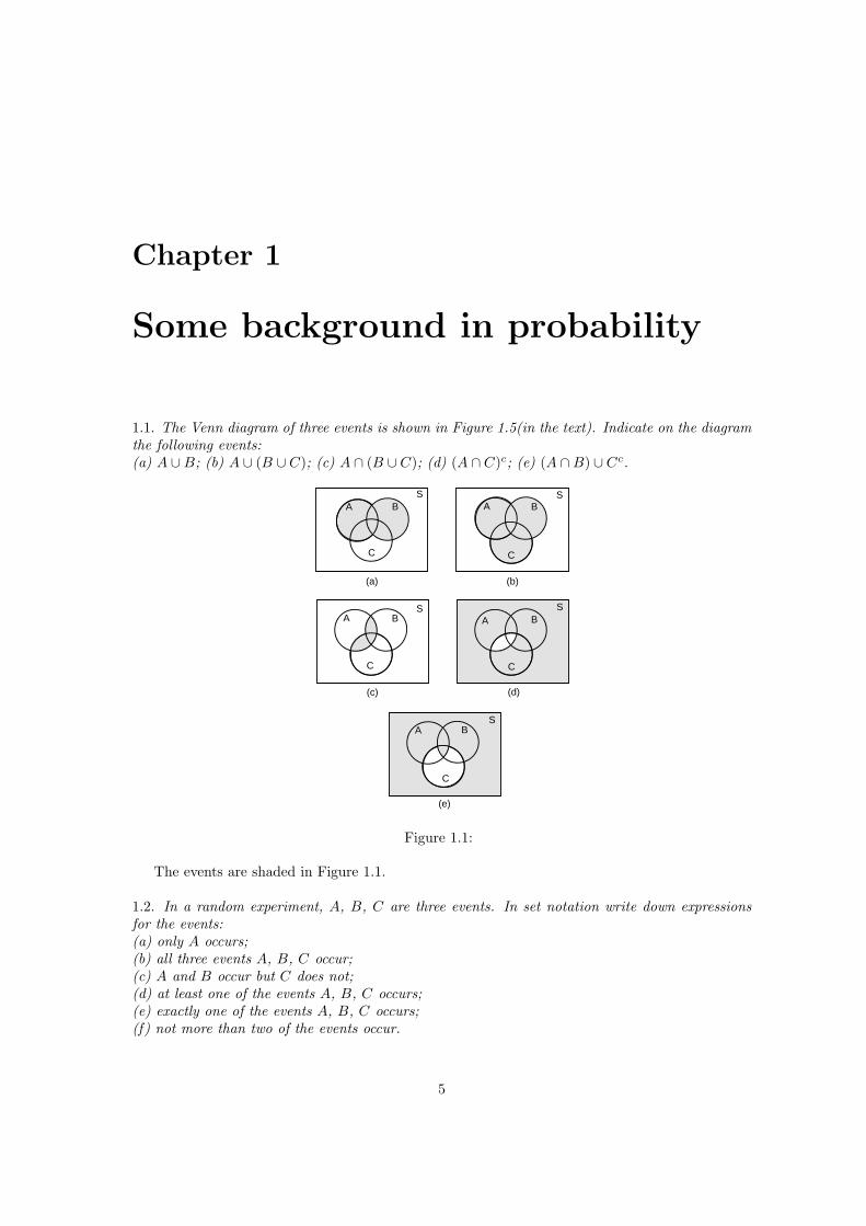
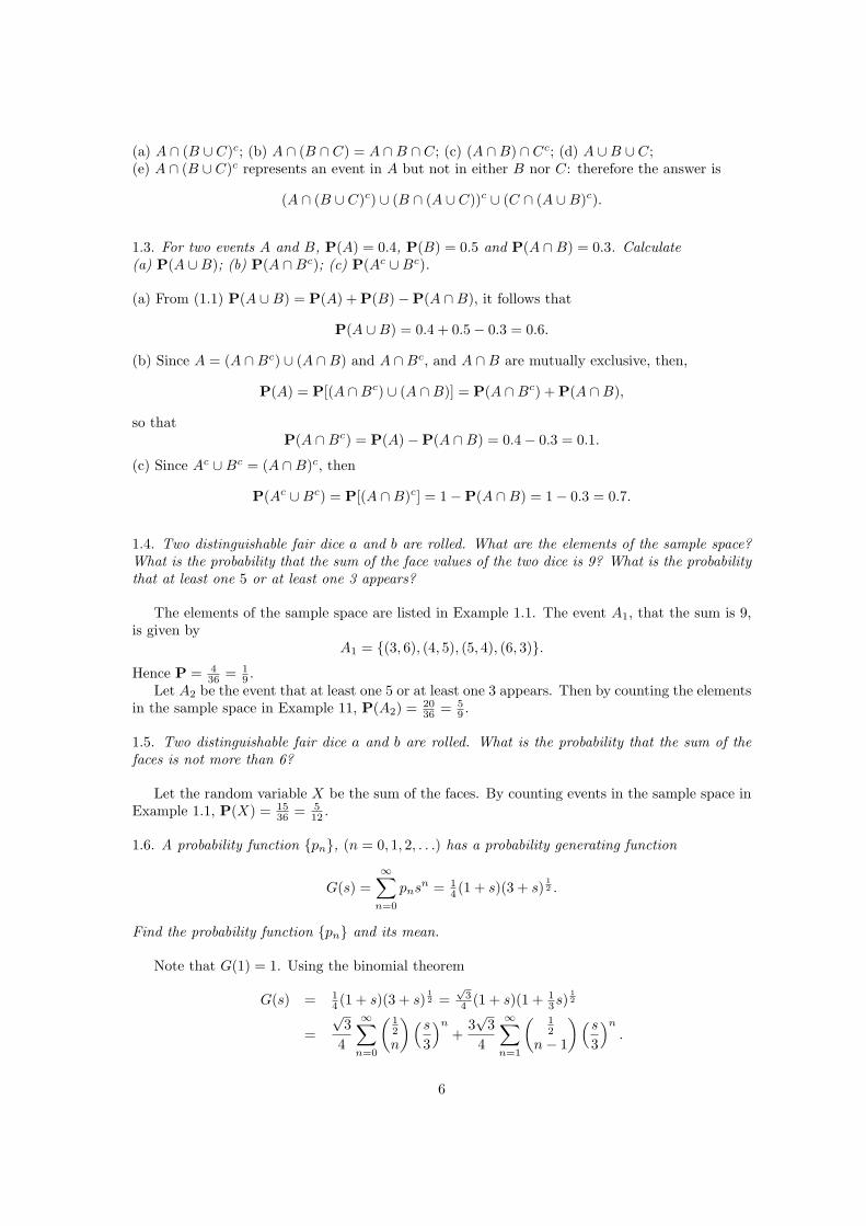
1.1. The Venn diagram of three events is shown in Figure 1.5(in the text). Indicate on the diagramthe following events:(a) A ∪B; (b) A ∪ (B ∪ C); (c) A ∩ (B ∪ C); (d) (A ∩ C)c; (e) (A ∩B) ∪ Cc.
(c)
(a) (b)
(d)
(e)
S S
S S
S
A A
A A
A
B B
B B
B
C C
C C
C
Figure 1.1:
The events are shaded in Figure 1.1.
1.2. In a random experiment, A, B, C are three events. In set notation write down expressionsfor the events:(a) only A occurs;(b) all three events A, B, C occur;(c) A and B occur but C does not;(d) at least one of the events A, B, C occurs;(e) exactly one of the events A, B, C occurs;(f) not more than two of the events occur.
5
(a) A ∩ (B ∪ C)c; (b) A ∩ (B ∩ C) = A ∩B ∩ C; (c) (A ∩B) ∩ Cc; (d) A ∪B ∪ C;(e) A ∩ (B ∪ C)c represents an event in A but not in either B nor C: therefore the answer is
(A ∩ (B ∪ C)c) ∪ (B ∩ (A ∪ C))c ∪ (C ∩ (A ∪B)c).
1.3. For two events A and B, P(A) = 0.4, P(B) = 0.5 and P(A ∩B) = 0.3. Calculate(a) P(A ∪B); (b) P(A ∩Bc); (c) P(Ac ∪Bc).
(a) From (1.1) P(A ∪B) = P(A) + P(B)−P(A ∩B), it follows that
P(A ∪B) = 0.4 + 0.5− 0.3 = 0.6.
(b) Since A = (A ∩Bc) ∪ (A ∩B) and A ∩Bc, and A ∩B are mutually exclusive, then,
P(A) = P[(A ∩Bc) ∪ (A ∩B)] = P(A ∩Bc) + P(A ∩B),
so thatP(A ∩Bc) = P(A)−P(A ∩B) = 0.4− 0.3 = 0.1.
(c) Since Ac ∪Bc = (A ∩B)c, then
P(Ac ∪Bc) = P[(A ∩B)c] = 1−P(A ∩B) = 1− 0.3 = 0.7.
1.4. Two distinguishable fair dice a and b are rolled. What are the elements of the sample space?What is the probability that the sum of the face values of the two dice is 9? What is the probabilitythat at least one 5 or at least one 3 appears?
The elements of the sample space are listed in Example 1.1. The event A1, that the sum is 9,is given by
A1 = {(3, 6), (4, 5), (5, 4), (6, 3)}.Hence P = 4
36 = 19 .
Let A2 be the event that at least one 5 or at least one 3 appears. Then by counting the elementsin the sample space in Example 11, P(A2) = 20
36 = 59 .
1.5. Two distinguishable fair dice a and b are rolled. What is the probability that the sum of thefaces is not more than 6?
Let the random variable X be the sum of the faces. By counting events in the sample space inExample 1.1, P(X) = 15
36 = 512 .
1.6. A probability function {pn}, (n = 0, 1, 2, . . .) has a probability generating function
G(s) =∞∑
n=0
pnsn = 14 (1 + s)(3 + s)
12 .
Find the probability function {pn} and its mean.
Note that G(1) = 1. Using the binomial theorem
G(s) = 14 (1 + s)(3 + s)
12 =
√3
4 (1 + s)(1 + 13s)
12
=√
34
∞∑n=0
( 12
n
) (s
3
)n
+3√
34
∞∑n=1
( 12
n− 1
) (s
3
)n
.
6
The probabilities can now be read off from the coefficients of the series:
p0 =√
34
, pn =√
33n4
[( 12
n
)+ 3
( 12
n− 1
)], (n = 1, 2, . . .).
The expected value is given by
µ = G′(1) =14
dds
[(1 + s)(3 + s)
12
]s=1
=[14(3 + s)
12 +
18(1 + s)(3 + s)−
12
]
s=1
=58
1.7. Find the probability generating function G(s) of the Poisson distribution (see Section 1.7) withparameter α given by
pn =e−ααn
n!, n = 0, 1, 2, . . . .
Determine the mean and variance of {pn} from the generating function.
Given pn = e−ααn/n!, the generating function is given by
G(s) =∞∑
n=0
pnsn =∞∑
n=0
e−ααnsn
n!= e−α
∞∑n=0
(αs)n
n!= eα(s−1).
The mean and variance are given by
µ = G′(1) =dds
[eα(s−1)
]s=1
= α,
σ2 = G′′(1) + G′(1)− [G′(1)]2 = [α2eα(s−1) + αeα(s−1) − α2e2α(s−1)]s=1 = α,
as expected.
1.8. A panel contains n warning lights. The times to failure of the lights are the independentrandom variables T1, T2, . . . , Tn which have exponential distributions with parameters α1, α2, . . . , αn
respectively. Let T be the random variable of the time to first failure, that is
T = min{T1, T2, . . . , Tn}.
Show that T has an exponential distribution with parameter∑n
j=1 αj. Show also that the probabilitythat the i-th panel light fails first is αi/(
∑nj=1 αj).
The probability that no warning light has failed by time t is
P(T ≥ t) = P(T1 ≥ t ∩ T2 ≥ t ∩ · · · ∩ Tn ≥ t)= P(T1 ≥ t)P(T2 ≥ t) · · ·P(Tn ≥ t)= e−α1te−α2t · · · e−αnt = e−(α1+α2+···+αn)t.
7
Let Ti represent the random variable that the ith component fails first. The probability thatthe ith component fails first is
P(Ti = T ) =∑
δt
∏
n6=i
P(Tn > t)P(t < Ti < t + δt)
=∑
δt
∏
n6=i
P(Tn > t)[e−αit − e−αi(t+δt)]
≈∑
δt
∏
n6=i
P(Tn > t)αiδte−αit
→∫ ∞
0
αi exp
[−t
n∑
i=1
αi
]dt =
αi∑ni=1 αi
as δt → 0.
1.9. The geometric probability function with parameter p is given by
p(x) = qx−1p, x = 1, 2, . . .
where q = 1 − p (see Section 1.7). Find its probability generating function. Calculate the meanand variance of the geometric distribution from its pgf.
The generating function is given by
G(s) =∞∑
x=1
qx−1psx =p
q
∞∑x=1
(qs)x =p
q
qs
1− qs=
ps
1− qs,
using the formula for the sum of a geometric series.The mean is given by
µ = G′(1) =dds
[ps
1− qs
]
s=1
=[
p
1− qs+
pqs
(1− qs)2
]
s=1
=1p.
For the variance,
G′′(s) =dds
[p
(1− qs)2
]=
2pq
(1− qs)3.
is required. Hence
σ2 = G′′(1) + G′(1)− [G′(1)]2 =2q
p2+
1p− 1
p2=
1− p
p2.
1.10. Two distinguishable fair dice a and b are rolled. What are the probabilities that:(a) at least one 4 appears;(b) only one 4 appears;(c) the sum of the face values is 6;(d) the sum of the face values is 5 and one 3 is shown;(e) the sum of the face values is 5 or only one 3 is shown?
From the Table in Example 1.1:(a) If A1 is the event that at least one 4 appears, then P(A1) = 11
36 .(b) If A2 is the event that only one 4 appears, then P(A2) = 10
36 = 518 .
(c) If A3 is the event that the sum of the faces is 6, then P(A3) = 536 .
8
(d) If A4 is the event that the face values is 5 and one 3 is shown, then P(A4) = 236 = 1
18 .(e) If A5 is the event that the sum of the faces is 5 or only one 3 is shown, then P(A5) = 7
36 .
1.11. Two distiguishable fair dice a and b are rolled. What is the expected sum of the face values?What is the variance of the sum of the face values?
Let N be the random variable representing the sum x + y, where x and y are face values of thetwo dice. Then
E(N) =136
6∑x=1
6∑y=1
(x + y) =136
[6
6∑x=1
x + 66∑
y=1
y
]= 7.
and
V(N) = E(N2)−E(N) =136
6∑x=1
6∑y=1
(x + y)2 − 72
=136
[12
6∑x=1
x2 + 2(6∑
x=1
x)2]− 49
=136
[(12× 91) + 2× 212]− 49 =356
= 5.833 . . . .
1.12. Three distinguishable fair dice a, b and c are rolled. How many possible outcomes are therefor the faces shown? When the dice are rolled, what is the probability that just two dice show thesame face values and the third one is different?
The sample space contains 63 = 216 elements of the form, (in the order a, b, c),
S = {(i, j, k)}, (i = 1, . . . , 6; j = 1, . . . , 6; k = 1, . . . , 6).
Let A be the required event. Suppose that a and b have the same face values, which can occur in6 ways, and that c has a different face value which can occurs in 5 ways. Hence the total numberof ways in which a and b are the same but c is different is 6 × 5 = 30 ways. The faces b and c,and c and a could also be the same so that the total number of ways for the possible outcome is3× 30 = 90 ways. Therefore the required probability is
P(A) =90216
=512
.
1.13. In a sample space S, the events B and C are mutually exclusive, but A and B, and A andC are not. Show that
P(A ∪ (B ∪ C)) = P(A) + P(B) + P(C)−P(A ∩ (B ∪ C)).
From a well-shuffled pack of 52 playing cards a single card is randomly drawn. Find the proba-bility that it is a club or an ace or the king of hearts.
From (1.1) (in the book)
P(A ∪ (B ∪ C)) = P(A) + P(B ∪ C)−P(A ∩ (B ∪ C)) (i).
Since B and C are mutually exclusive,
P(B ∪ C) = P(B) + P(C). (ii)
9
From (i) and (ii), it follows that
P(A ∪ (B ∪ C)) = P(A) + P(B) + P(C)−P(A ∩ (B ∪ C)).
Let A be the event that the card is a club, B the event that it is an ace, and C the event thatit is the king of hearts. We require P(A∪ (B ∪C)). Since B and C are mutually exclusive, we canuse the result above. The individual probabilities are
P(A) =1352
=14; P(B) =
452
=113
; P(C) =152
,
and since A ∩ (B ∪ C) is the ace of clubs,
P(A ∩ (B ∪ C)) =152
.
Finally
P(A ∪ (B ∪ C)) =14
+113
+152− 1
52=
1752
.
1.14. Show that
f(x) =
0 x < 012a 0 ≤ x ≤ a12ae−(x−a)/a x > a
is a possible probability density function. Find the corresponding probability function.
Check the density function as follows:∫ ∞
−∞f(x)dx =
12a
∫ a
0
dx +12a
∫ ∞
a
e−(x−a)/adx
= 12 − 1
2 [e−(x−a)/a]∞a = 1.
The probability function is given by, for 0 ≤ x ≤ a,
F (x) =∫ x
−∞f(u)du =
∫ x
0
12a
du =x
2a,
and, for x > a, by
F (x) =∫ x
0
f(u)du =∫ a
0
12a
du +∫ a
0
12a
e−(u−a)/adu
=12− 1
2a[ae−(u−a)/a]xa
= 1− 12e−(x−a)/a.
1.15. A biased coin is tossed. The probability of a head is p. The coin is tossed until the first headappears. Let the random variable N be the total number of tosses including the first head. FindP(N = n), and its pgf G(s). Find the expected value of the number of tosses.
The probability that the total number of throws is n (including the head) until the first headappears is
P(N = n) =
(n−1) times︷ ︸︸ ︷(1− p)(1− p) · · · (1− p) p = (1− p)n−1p, (n ≥ 1)
10
The probability generating function is given by
G(s) =∞∑
n=1
(1− p)n−1psn =p
1− p
∞∑n=1
[(1− p)s]n
=p
1− p· s(1− p)[1− s(1− p)]
=ps
1− s(1− p),
after summing the geometric series.For the mean, we require G′(s) given by,
G′(s) =p
[1− s(1− p)]+
sp(1− p)[1− s(1− p)]2
=p
[1− s(1− p)]2.
The mean is given by µ = G′(1) = 1/p.
1.16. The n random variables X1, X2, . . . , Xm are independent and identically distributed each witha gamma distribution with parameters n and α. The random variable Y is defined by
Y = X1 + X2 + · · ·+ Xm.
Using the moment generating function, find the mean and variance of Y .
The probability density function for the gamma distribution with parameters n and α is
f(x) =αn
Γ(n)xn−1e−αx.
It was shown in Section 1.9 that the moment generating function for Y is given, in general, by
MY (s) = [MX(s)]m,
where X has a gamma distribution with the same parameters. Hence
MY (s) =(
α
α− s
)nm
=(1− s
α
)nm
= 1 +nm
αs +
nm(nm + 1)2α2
s2 + · · ·
HenceE(Y ) =
nm
α, V(Y ) = E(Y 2)− [E(Y )]2 =
nm
α2.
1.17. A probability generating function with parameter 0 < α < 1 is given by
G(s) =1− α(1− s)1 + α(1− s)
.
Find pn = P(N = n) by expanding the series in powers of s. What is the mean of the probabilityfunction {pn}?
Applying the binomial theorem
G(s) =1− α(1− s)1 + α(1− s)
=(1− α)[1 + (α/(1− α))s](1 + α)[1− (α/(1 + α))s]
=(
1− α
1 + α
)(1 +
αs
1− α
) ∞∑n=
(αs
1 + α
)n
=1− α
1 + α
∞∑n=0
(α
1 + α
)n
sn +α
1 + α
∞∑n=0
(α
1 + α
)n
sn+1.
11
The summation of the two series leads to
G(s) =1− α
1 + α
∞∑n=0
(α
1 + α
)n
sn +∞∑
n=1
(α
1 + α
)n
sn
=1− α
1 + α+
21 + α
∞∑n=1
(α
1 + α
)n
sn
Hencep0 =
1 + α
1− α, pn =
2αn
(1 + α)n+1, (n = 1, 2, . . .).
The mean is given by
G′(1) =dds
[1− α(1− s)1 + α(1− s)
]
s=1
=[
2α
[1 + a(1− s)]2
]
s=1
= 2α
1.18. Find the moment generating function of the random variables X which has the uniformdistribution
f(x) ={
1/(b− a) a ≤ x ≤ b0 for all other values of x
Deduce E(Xn).
The moment generating function of the uniform distribution is
MX(s) =∫ b
a
exs
b− adx =
1b− a
1s[ebs − eas]
=1
b− a
∞∑n=1
(bn − an
n!
)sn−1
Hence
E(X) =12(b + a), E(Xn) =
bn+1 − an+1
(n + 1)(b− a).
1.19. A random variable X has the normal distribution N(µ, σ2). Find its momemt generatingfunction.
By definition
MX(s) = E(eXs) =1
σ√
2π
∫ ∞
−∞esx exp
[− (x− µ)2
2σ2
]dx
=1
σ√
2π
∫ ∞
−∞exp
[2σ2xs− (x− µ)2
2σ2
]dx
Apply the substitution x = µ + σ(v − σs): then
MX(s) = exp(sµ + 12σ2s2)
∫ ∞
−∞
1√2π
e−12 v2
dv
= exp(sµ + 12σ2s2) + 1 = exp(sµ + 1
2σ2s2)
(see the Appendix for the integral).
12
Expansion of the exponential function in powers of s gives
MX(s) = 1 + µs +12(σ2 + µ2)s2 + · · · .
So, for example, E(X2) = µ2 + σ2.
1.20. Find the probability generating functions of the following distributions, in which 0 < p < 1:(a) Bernoulli distribution: pn = pn(1− p)n, (n = 0, 1);(b) geometric distribution: pn = p(1− p)n−1, (n = 1, 2, . . .);(c) negative binomial distribution with parameter r expressed in the form:
pn =(
r + n− 1r − 1
)pr(1− p)n, (n = 0, 1, 2, . . .)
where r is a positive integer. In each case find also the mean and variance of the distribution usingthe probability generating function.
(a) For the Bernoulli distribution
G(s) = p0 + p1s = (1− p) + ps.
The mean is given byµ = G′(1) = p,
and the variance by
σ2 = G′′(1) + G′(1)− [G′(1)]2 = p− p2 = p(1− p).
(b) For the geometric distribution (with q = 1− p)
G(s) =∞∑
n=1
pqn−1sn = ps
∞∑n=0
(qs)n =ps
1− qs
summing the geometric series. The mean and variance are given by
µ = G′(1) =[
p
1− qs
]
s=1
=1p,
σ2 = G′′(1) + G′(1)− [G′(1)]2 =[
2pq
(1− qs)3
]
s=1
+1p− 1
p2=
1− p
p2.
(c) For the negative binomial distribution (with q = 1− p)
G(s) =∞∑
n=0
(r + n− 1
r − 1
)prqnsn = pr
(1 + r(qs) +
r(r + 1)2!
(qs)2 + · · ·)
=pr
(1− qs)r
The derivatives of G(s) are given by
G′(s) =rqpr
(1− qs)r+1, G′′(s) =
r(r + 1)q2pr
(1− qs)r+2.
Hence the mean and variance are given by
µ = G′(1) =rq
p,
13
σ2 = G′′(1) + G′(1)− [G′(1)]2 =r(r + 1)q2
p2+
rq
p− r2q2
p2=
rq
p2
1.21. A word of five letters is transmitted by code to a receiver. The transmission signal is weak,and there is a 5% probability that any letter is in error independently of the others. What is theprobability that the word is received correctly? The same word is transmitted a second time withthe same errors in the signal. If the same word is received, what is the probability now that theword is correct?
Let A1, A2, A3, A4, A5 be the events that the letters in the word are correct. Since the eventsare independent, the probability that the word is correctly transmitted is
P(A1 ∩A2 ∩A3 ∩A4 ∩A5) = 0.955 ≈ 0.774.
If a letter is sent a second time the probability that one error occurs twice is 0.052 = 0.0025.Hence the probability that the letter is correct is 0.9975. For 5 letters the probability that theword is correct is 0.99755 ≈ 0.988.
1.22. A random variable N over the positive integers has the probability distribution with
pn = P(N = n) = − αn
n ln(1− α), (0 < α < 1; n = 1, 2, 3, . . .).
What is its probability generating function? Find the mean of the random variable.
The probability generating function is given by
G(s) = −∞∑
n=1
αnsn
n log(1− α)=
log(1− αs)log(1− α)
for 0 ≤ s < 1/α.Since
G′(s) =−α
(1− αs) log(1− α),
the mean isµ = G′(1) =
−α
(1− α) log(1− α).
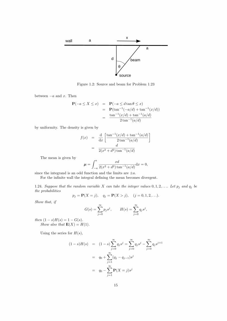
1.23. The source of a beam of light is a perpendicular distance d from a wall of length 2a, withthe perpendicular from the source meeting the wall at its midpoint. The source emits a pulse oflight randomly in a direction θ, the angle between the direction of the pulse and the perpendicularis chosen uniformly in the range − tan−1(a/d) ≤ θ ≤ tan−1(a/d). Find the probability distributionof x (−a ≤ x ≤ a) where the pulses hit the wall. Show that its density function is given by
f(x) =d
2(x2 + d2) tan−1(a/d),
(this the density function of a Cauchy distribution). If a → ∞, what can you say about themean of this distribution?
Figure 1.2 shows the beam and wall. Let X be the random variable representing any displacement
14
x
d
a
a
θ
source
wall
beam
Figure 1.2: Source and beam for Problem 1.23
between −a and x. Then
P(−a ≤ X ≤ x) = P(−a ≤ d tan θ ≤ x)= P(tan−1(−a/d) + tan−1(x/d))
=tan−1(x/d) + tan−1(a/d)
2 tan−1(a/d)
by uniformity. The density is given by
f(x) =ddx
[tan−1(x/d) + tan−1(a/d)
2 tan−1(a/d)
]
=d
2(x2 + d2) tan−1(a/d)
The mean is given by
µ =∫ a
−a
xd
2(x2 + d2) tan−1(a/d)dx = 0,
since the integrand is an odd function and the limits are ±a.For the infinite wall the integral defining the mean becomes divergent.
1.24. Suppose that the random variable X can take the integer values 0, 1, 2, . . .. Let pj and qj bethe probabilities
pj = P(X = j), qj = P(X > j), (j = 0, 1, 2, . . .).
Show that, if
G(s) =∞∑
j=0
pjsj , H(s) =
∞∑
j=0
qjsj ,
then (1− s)H(s) = 1−G(s).Show also that E(X) = H(1).
Using the series for H(s),
(1− s)H(s) = (1− s)∞∑
j=0
qjsj =
∞∑
j=0
qjsj −
∞∑
j=0
qjsj+1
= q0 +∞∑
j=1
(qj − qj−1)sj
= q0 −∞∑
j=1
P(X = j)sj
15
= 1− p0 −∞∑
j=1
pjsj = 1−G(s)
Note that generally H(s) is not a probability generating function.The mean of the random variable X is given by
E(X) =∞∑
j=1
jpj = G′(1) = H(1),
differentiating the formula above.
16
Chapter 2
Some gambling problems
2.1. In the standard gambler’s ruin problem with total stake a and gambler’s stake k and thegambler’s probability of winning at each play is p, calculate the probability of ruin in the followingcases;(a) a = 100, k = 5, p = 0.6;(b) a = 80, k = 70, p = 0.45;(c) a = 50, k = 40, p = 0.5.Also find the expected duration in each case.
For p 6= 12 , the probability of ruin uk and the expected duration of the game dk are given by
uk =sk − sa
1− sa, dk =
11− 2p
[k − a(1− sk)
(1− sa)
].
(a) uk ≈ 0.132, dk ≈ 409.(b) uk ≈ 0.866, dk ≈ 592.(c) For p = 1
2 ,
uk =a− k
a, dk = k(a− k).
so that uk = 0.2, dk = 400.
2.2. In a casino game based on the standard gambler’s ruin, the gambler and the dealer each startwith 20 tokens and one token is bet on at each play. The game continues until one player has nofurther tokens. It is decreed that the probability that any gambler is ruined is 0.52 to protect thecasino’s profit. What should the probability that the gambler wins at each play be?
The probability of ruin is
u =sk − sa
1− sa,
where k = 20, a = 40, p is the probability that the gambler wins at each play, and s = (1− p)/p.Let r = s20. Then u = r/(1 + r), so that r = u/(1− u) and
s =(
u
1− u
)1/20
.
Finally
p =1
1 + s=
(1− u)1/20
(1− u)1/20 + u1/20≈ 0.498999.
17
2.3. Find general solutions of the following difference equations:(a) uk+1 − 4uk + 3uk−1 = 0;(b) 7uk+2 − 8uk+1 + uk = 0;(c) uk+1 − 3uk + uk−1 + uk−2 = 0.(d) puk+2 − uk + (1− p)uk−1 = 0, (0 < p < 1).
(a) The characteristic equation ism2 − 4m + 3 = 0
which has the solutions m1 = 1 and m2 = 3. The general solution is
uk = Amk1 + Bmk
2 = A + B.3k,
where A and B are any constants.(b) The characteristic equation is
7m2 − 8m + 1 = 0,
which has the solutions m1 = 1 and m2 = 17 . The general solution is
uk = A + B17k
.
(c) The characteristic equation is the cubic equation
m3 − 3m2 + m + 1 = (m− 1)(m2 − 2m + 1) = 0,
which has the solutions m1 = 1, m2 = 1 +√
2, and m3 = 1−√2. The general solution is
uk = A + B(1 +√
2)k + C(1−√
2)k.
(d) The characteristic equation is the cubic equation
pm3 −m + (1− p) = (m− 1)(pm2 + pm− (1− p)) = 0,
which has the solutions m1 = 1, m2 = − 12 + 1
2
√[(4− 3p)/p] and m3 = − 1
2 − 12
√[(4− 3p)/p]. The
general solution isuk = A + Bmk
2 + Cmk3 .
2.4 Solve the following difference equations subject to the given boundary conditions:(a) uk+1 − 6uk + 5uk−1 = 0, u0 = 1, u4 = 0;(b) uk+1 − 2uk + uk−1 = 0, u0 = 1, u20 = 0;(c) dk+1 − 2dk + dk−1 = −2, d0 = 0, d10 = 0;(d) uk+2 − 3uk + 2uk−1 = 0, u0 = 1, u10 = 0, 3u9 = 2u8.
(a) The charactedristic equation ism2 − 6m + 5 = 0,
which has the solutions m1 = 1 and m2 = 5. Therefore the general solution is given by
uk = A + 5kB.
The boundary conditions u0 = 1, u4 = 0 imply
A + B = 1, A + 54B = 0,
18
which have the solutions A = 625/624 and B = −1/624. The required solution is
uk =625624
− 5k
624.
(b) The characteristic equation is
m2 − 2m + 1 = (m− 1)2 = 0,
which has one solution m = 1. Using the rule for repeated roots,
uk = A + Bk.
The boundary conditions u0 = 1 and u20 = 0 imply A = 1 and B = −1/20. The required solutionis uk = (20− k)/20.(c) This is an inhomogeneous equation. The characteristic equation is
m2 − 2m + 1 = (m− 1)2 = 0,
which has the repeated solution m = 1. Hence the complementary function is A + Bk. For aparticular solution, we must try uk = Ck2. Then
dk+1 − 2dk + dk−1 = C(k + 1)2 − 2Ck2 + C(k − 1)2 = 2C = −2
if C = −1. Hence the general solution is
uk = A + Bk − k2.
The boundary conditions d0 = d10 = 0 imply A = 0 and B = 10. Therefore the required solutionis uk = k(10− k).(d) The characteristic equation is
m3 − 3m + 2 = (m− 1)2(m + 2) = 0,
which has two solutions m1 = 1 (repeated) and m2 = −2. The general solution is given by
uk = A + Bk + C(−2)k.
The boundary conditions imply
A + C = 1, A + 10B + C(−2)10 = 0, 3A + 27B + 3C(−2)9 = 2[A + 8B + C(−2)8].
The solutions of these linear equations are
A =3174431743
, B =307231743
, C = − 131743
so that the required solution is
uk =1024(31− 2k)− (−2)k
31743.
2.5. Show that a difference equation of the form
auk+2 + buk+1 − uk + cuk−1 = 0,
where a, b, c ≥ 0 are probabilities with a + b + c = 1, can never have a characteristic equation withcomplex roots.
19
The characteristic equation can be expressed in the form
am3 + bm2 −m + c = (m− 1)[am2 + (a + b)m− (1− a− b)] = 0,
since a + b + c = 1. One solution is m1 = 1, and the others satisfy the quadratic equation
am2 + (a + b)m− (1− a− b) = 0.
The discriminant is given by
(a + b)2 + 4(1− a− b) = (a− b)2 + 4a(1− a) ≥ 0,
since a ≤ 1.
2.6. In the standard gambler’s ruin problem with equal probabilities p = q = 12 , find the expected
duration of the game given the usual initial stakes of k units for the gambler and a − k units forthe opponent.
The expected duration dk satisfies
dk+1 − 2dk + dk−1 = −2.
The complementary function is A + Bk, and for a particular solution try dk = Ck2. Then
dk+1 − 2dk + dk−1 + 2 = C(k + 1)2 − 2Ck2 + C(k − 1)2 + 2 = 2C + 2 = 0
if C = −1. Hencedk = A + Bk − k2.
The boundary conditions d0 = da = 0 imply A = 0 and B = a. The required solution is therefore
dk = k(a− k).
2.7. In a gambler’s ruin problem the possibility of a draw is included. Let the probability that thegambler wins, loses or draws against an opponent be respectively, p, p, 1−2p, (0 < p < 1
2 ). Find theprobability that the gambler loses the game given the usual initial stakes of k units for the gamblerand a− k units for the opponent. Show that dk, the expected duration of the game, satisfies
pdk+1 − 2pdk + pdk−1 = −1.
Solve the difference equation and find the expected duration of the game.
The difference equation for the probability of ruin uk is
uk = puk+1 + (1− 2p)uk + puk−1 or uk+1 − 2uk + uk−1 = 0.
The general solution is uk = A + Bk. The boundary conditions u0 = 1 and ua = 0 imply A = 1and B = −1/a, so that the required probability is given by uk = (a− k)/a.
The expected duration dk satisfies
dk+1 − 2dk + dk+1 = −1/p.
The complementary function is A + Bk. For the particular solution try dk = Ck2. Then
C(k + 1)2 − 2Ck2 + C(k − 1)2 = 2C = −1/p
20
if C = −1/(2p). The boundary conditions d0 = da = 0 imply A = 0 and B = a/(2p), so that therequired solution is
dk = k(a− 2p)/(2p).
2.8. In the changing stakes game in which a game is replayed with each player having twice asmany units, 2k and 2(a − k) respectively, suppose that the probability of a win for the gambler ateach play is 1
2 . Whilst the probability of ruin is unaffected by how much is the expected duration ofthe game extended compared with the original game?
With initial stakes of k and a− k, the expected duration is dk = k(a− k). If the initial stakesare doubled to 2k and 2a− 2k, then the expected duration becomes, using the same formula,
d2k = 2k(2a− 2k) = 4k(a− k) = 4dk.
2.9. A roulette wheel has 37 radial slots of which 18 are red, 18 are black and 1 is green. Thegambler bets one unit on either red or black. If the ball falls into a slot of the same colour, thenthe gambler wins one unit, and if the ball falls into the other colour (red or black), then the casinowins. If the ball lands in the green slot, then the bet remains for the next spin of the wheel ormore if necessary until the ball lands on a red or black. The original bet is either returned or lostdepending on whether the outcome matches the original bet or not (this is the Monte Carlo system).Show that the probability uk of ruin for a gambler who starts with k chips with the casino holdiinga− k chips satisfies the difference equation
36uk+1 − 73uk + 37uk−1 = 0.
Solve the difference equation for uk. If the house starts with ∈1,000,000 at the roulette wheel andthe gambler starts with ∈10,000, what is the probability that the gambler breaks the bank if ∈5,000are bet at each play.
In the US system the rules are less generous to the players. If the ball lands on green then theplayer simply loses. What is the probability now that the player wins given the same initial stakes?(see Luenberger (1979))
There is the possibility of a draw (see Example 2.1). At each play the probability that thegambler wins is p = 18
37 . The stake is returned with probability
137
(1837
)+
1372
(1837
)+ · · · = 1
361837
=174
,
or the gambler loses after one or more greens also with probability 1/74 by the same argument.Hence uk, the probability that the gambler loses satisfies
uk =1837
uk+1 +174
(uk + uk−1) +1837
uk+1,
or36uk+1 − 73uk + 37uk−1 = 0.
The charactersitic equation is
36m2 − 73m + 37 = (m− 1)(36m− 37) = 0,
which has the solutions m1 = 1 and m2 = 37/36. With u0 = 1 and ua = 0, the required solution is
uk =sk − sa
1− sa, s =
3736
.
21
The bets are equivalent to k = 10000/5000 = 2, a = 1010000/5000 = 202. The probability thatthe gambler wins is
1− uk =1− sk
1− sa=
1− s2
1− s202= 2.23× 10⁻⁴.
In the US system, uk satisfies
uk =1837
uk+1 +1937
uk−1, or 18uk+1 − 37uk + 19uk−1 = 0.
in this case the ratio is s′ = 19/18. Hence the probability the the gambler wins is
1− uk =1− s′2
1− s′202= 2.06× 10⁻⁶,
which is less than the previous value.
2.10. In a single trial the possible scores 1 and 2 can occur each with probability 12 . If pn is the
probability of scoring exactly n points at some stage, show that
pn = 12pn−1 + 1
2pn−2.
Calculate p1 and p2, and find a formula for pn. How does pn behave as n becomes large? How doyou interpret the result?
Let An be the event that the score is n at some stage. Let B1 be the event score 1, and B2
score 2. Then
P(An) = P(An|B1)P(B1) + P(An|B2)P(B2) = P(An−1) 12 + P(An−2) 1
2 ,
orpn = 1
2pn−1 + 12pn−2.
Hence2pn − pn−1 − pn−2 = 0.
The characteristic equation is
2m2 −m− 1 = (m− 1)(2m + 1) = 0,
which has the solutions m1 = 1 and m2 = − 12 . Hence
pn = A + B(− 12 )n.
The initial conditions are p1 = 12 and p2 = 1
2 + 12
12 = 3
4 . Hence
A− 12B = 1
2 , A + 14B = 3
4 ,
so that A = 23 , B = 1
3 . Hence
pn = 23 + 1
3 (− 12 )n, (n = 1, 2, . . .).
As n →∞, pn → 23 .
2.11. In a single trial the possible scores 1 and 2 can occur with probabilities q and 1 − q, where0 < p < 1. Find the probability of scoring exactly n points at some stage in an indefinite successionof trials. Show that
pn → 12− p
,
22
as n →∞.
Let pn be the probability. Then
pn = qpn−1 + (1− q)pn−2, or pn − qpn−1 − (1− q)pn−2 = 0.
The characteristic equation is
m2 − qm− (1− q) = (m− 1)[m + (1− q)] = 0,
which has the solutions m1 = 1 and m2 = −(1− q). Hence
pn = A + B(q − 1)n.
The initial conditions are p1 = q, p2 = 1− q + q2, which imply
q = A + B(q − 1), 1− q + q2 = A + B(q − 1)2.
The solution of these equations leads to A = 1/(2− q) and B = (q − 1)/(q − 2), so that
pn =1
2− q[1− (q − 1)n+1].
2.12. The probability of success in a single trial is 13 . If un is the probability that there are no two
consecutive successes in n trials, show that un satisfies
un+1 = 23un + 2
9un−1.
What are the values of u1 and u2? Hence show that
un =16
[(3 + 2
√3)
(1 +
√3
3
)n
+ (3− 2√
3)
(1−√3
3
)n].
Let An be the event that there have not been two consecutive successes in the first n trials.Let B1 be the event of success and B2 the event of failure. Then
P(An) = P(An|B1)P(B1) + P(An|B2)P(B2).
Now P(An|B2) = P(An−1): failure will not change the probability. Also
P(An|B1) = P(An−1|B2)P(B2) = P(An−2)P(B2).
Since P(B1) = 13 , P(B2) = 2
3 ,
un = 29un−2 + 2
3un−1 or 9un − 6un−1 − 2un = 0,
where un = P(An).The characteristic equation is
9m2 − 6m− 2 = 0,
which has the solutions m1 = 13 (1 +
√3) and m2 = 1
3 (1−√3). Hence
un = A13n
(1 +√
3)n + B13n
(1−√
3)n.
23
The initial conditions are u1 = 1 and u2 = 1− 13
13 = 8
9 . Therefore A and B are defined by
1 =A
3(1 +
√3) +
B
3(1−
√3),
89
=A
9(1 +
√3)2 +
B
9(1−
√3)2 =
A
9(4 + 2
√3) +
B
9(4− 2
√3).
The solutions are A = 16 (2
√3 + 3) and B = 1
6 (−2√
3 + 3). Finally
un =1
6 · 3n[(2√
3 + 3)(1 +√
3)n + (−2√
3 + 3)(1−√
3)n].
2.13. A gambler with initial capital k units plays against an opponent with initial capital a − kunits. At each play of the game the gambler either wins one unit or loses one unit with probability12 . Whenever the opponent loses the game, the gambler returns one unit so that the game maycontinue. Show that the expected duration of the game is k(2a− 1− k) plays.
The expected duration dk satisfies
dk+1 − 2dk + dk−1 = −2, (k = 1, 2, . . . , a− 1).
The boundary conditions are d0 = 0 and da = da−1, indicating the return of one unit when thegambler loses. The general solution for the duration is
dk = A + Bk − k2.
The boundary conditions imply
A = 0, A + Ba− a2 = A + B(a− 1)− (a− 1)2,
so that B = 2a− 1. Hence dk = k(2a− 1− k).
2.14. In the usual gambler’s ruin problem, the probability that the gambler is eventually ruined is
uk =sk − sa
1− sa, s =
q
p, (p 6= 1
2 ).
In a new game the stakes are halved, whilst the players start with the same initial sums. How doesthis affect the probability of losing by the gambler? Should the gambler agree to this change of ruleif p < 1
2? By how many plays is the expected duration of the game extended?
The new probability of ruin vk (with the stakes halved) is, adapting the formula for uk,
vk = u2k =s2k − s2a
1− s2a=
(sk + sa)(sk − sa)(1− sa)(1 + sa)
= uk
(sk + sa
1 + sa
).
Given p < 12 , then s = (1− p)/p > 1 and sk > 1. It follows that
vk > uk
(1 + sa
1 + sa
)= uk.
With this change the gambler is more likely to lose.From (2.9), the expected duration of the standard game is given by
dk =1
1− 2p
[k − a(1− sk)
(1− sa)
].
24
With the stakes halved the expected duration hk is
hk = d2k =1
1− 2p
[2k − 2a(1− s2k)
(1− s2a)
].
The expected duration is extended by
hk − dk =1
1− 2p
[k − 2a(1− s2k)
(1− s2a)+
a(1− sk)(1− sa)
]
=1
1− 2p
[k +
a(1− sk)(sa − 1− 2sk)(1− s2a)
].
2.15. In a gambler’s ruin game, suppose that the gambler can win £2 with probability 13 or lose £1
with probability 23 . Show that
uk =(3k − 1− 3a)(−2)a + (−2)k
1− (3a + 1)(−2)a.
Compute uk if a = 9 for k = 1, 2, . . . , 8.
The probability of ruin uk satisfies
uk = 13uk+2 + 2
3uk−1 or uk+2 − 3uk + 2uk = 0.
The characteristic equation is
m3 − 3m + 2 = (m− 1)2(m + 2) = 0,
which has the solutions m1 = 1 (repeated) and m2 = −2. Hence
uk = A + Bk + C(−2)k.
The boundary conditions are u0 = 1, ua = 0, ua−1 = 23ua−2. The constants A, B and C satisfy
A + C = 1, A + Ba + C(−2)a = 0,
3[A + B(a + 1) + C(−2)a−1] = 2[A + B(a− 2) + C(−2)a−2],
orA + B(a + 1)− 8C(−2)a−2 = 0.
The solution of these equations is
A =−(−2)a(3a + 1)
1− (−2)a(3a + 1), B =
3(−2)a
1− (−2)a(3a + 1), C =
11− (−2)a(3a + 1)
.
Finally
uk =(3k − 1− 3a)(−2)a + (−2)k
1− (−2)a(3a + 1).
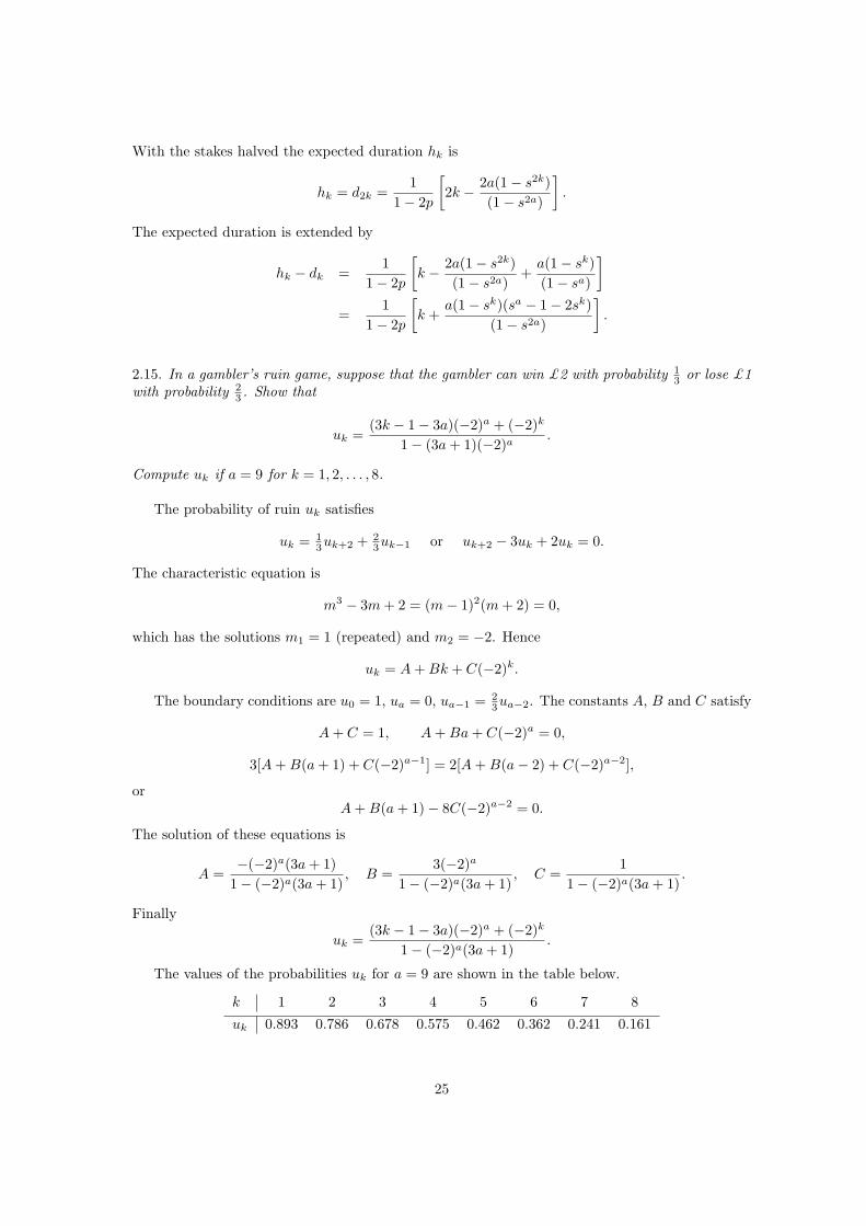
The values of the probabilities uk for a = 9 are shown in the table below.
k 1 2 3 4 5 6 7 8
uk 0.893 0.786 0.678 0.575 0.462 0.362 0.241 0.161
25
2.16. Find the general solution of the difference equation
uk+2 − 3uk + 2uk−1 = 0.
A reservoir with total capacity of a volume units of water has, during each day, either a netinflow of two units with probability 1
3 or a net outflow of one unit with probability 23 . If the
reservoir is full or nearly full any excess inflow is lost in an overflow. Derive a difference equationfor this model for uk, the probability that the reservoir will eventually become empty given that itinitially contains k units. Explain why the upper boundary conditions can be written ua = ua−1
and ua = ua−2. Show that the reservoir is certain to be empty at some time in the future.
The characteristic equation is
m3 − 3m + 2 = (m− 1)2(m + 2) = 0.
The general solution is (see Problem 2.15)
uk = A + Bk + C(−1)k.
The boundary conditions for the reservoir are
u0 = 1, ua = 13ua + 2
3ua−1, ua−1 = 13ua + 2
3ua−2.
The latter two conditions are equivalent to ua = ua−1 = ua−2. Hence
A + C = 1, A + Ba + C(−2)a = A + B(a− 1) + C(−2)a−1 = A + B(a− 2) + C(−2)a−2.
which have the solutions A = 1, B = C = 0. The solution is uk = 1, which means that that thereservoir is certain to empty at some future date.
2.17. Consider the standard gambler’s ruin problem in which the total stake is a and gambler’sstake is k, and the gambler’s probability of winning at each play is p and losing is q = 1− p. Finduk, the probability of the gambler losing the game, by the following alternative method. List thedifference equation (2.2) as
u2 − u1 = s(u1 − u0) = s(u1 − 1)u3 − u2 = s(u2 − u1) = s2(u1 − 1)
...uk − uk−1 = s(uk−1 − uk−2) = sk−1(u1 − 1),
where s = q/p 6= 12 and k = 2, 3, . . . a. The boundary condition u0 = 1 has been used in the first
equation. By adding the equations show that
uk = u1 + (u1 − 1)s− sk
1− s.
Determine u1 from the other boundary condition ua = 0, and hence find uk. Adapt the samemethod for the special case p = q = 1
2 .
Addition of the equations gives
uk − u1 = (u1 − 1)(s + s2 + · · ·+ sk−1) = (u1 − 1)s− sk
1− s
26
summing the geometric series. The condition ua = 0 implies
−u1 = (u1 − 1)s− sa
1− s.
Henceu1 =
s− sa
1− sa,
so that
uk =sk − sa
1− s.
2.18. A car park has 100 parking spaces. Cars arrive and leave randomly. Arrivals or departuresof cars are equally likely, and it is assumed that simultaneous events have negligible probability.The ‘state’ of the car park changes whenever a car arrives or departs. Given that at some instantthere are k cars in the car park, let uk be the probability that the car park first becomes full beforeit becomes empty. What are the boundary conditions for u0 and u100? How many car movementscan be expected before this occurs?
The probability uk satisfies the difference equation
uk =12uk+1 +
12uk−1 or uk+1 − 2uk + uk−1.
The general solution is uk = A + Bk. The boundary conditions are u0 = 0 and u100 = 1. HenceA = 0 and B = 1/100, and uk = k/100.
The expected duration of car movements until the car park becomes full is dk = k(100− k).
2.19. In a standard gambler’s ruin problem with the usual parameters, the probability that thegambler loses is given by
uk =sk − sa
1− sa, s =
1− p
p.
If p is close to 12 , given say by p = 1
2 + ε where |ε| is small, show, by using binomial expansions,that
uk =a− k
a
[1− 2kε− 4
3(a− 2k)ε2 + O(ε3)
]
as ε → 0. (The order O terminology is defined as follows: we say that a function g(ε) = O(εb) asε → 0 if g(ε)/εb is bounded in a neighbourhood which contains ε = 0. See also the Appendix in thebook.)
Let p = 12 + ε. Then s = (1− 2ε)/(1 + 2ε), and
uk =(1− 2ε)k(1 + 2ε)−k − (1− 2ε)a(1 + 2ε)−a
1− (1− 2ε)a(1 + 2ε)−a.
Apply the binomial theorem to each term. The result is
uk =a− k
a
[1− 2kε− 4
3(a− 2k)ε2 + O(ε3)
].
[Symbolic computation of the series is a useful check.]
2.20. A gambler plays a game against a casino according to the following rules. The gambler andcasino each start with 10 chips. From a deck of 53 playing cards which includes a joker, cards are
27
randomly and successively drawn with replacement. If the card is red or the joker the casino wins 1chip from the gambler, and if the card is black the gambler wins 1 chip from the casino. The gamecontinues until either player has no chips. What is the probability that the gambler wins? Whatwill be the expected duration of the game?
From (2.4) the probability uk that the gambler loses is (see (2.4))
uk =sk − sa
1− sa,
with k = 10, a = 20, p = 26/53, and s = 27/26. Hence
u10 =(27/26)10 − (27/26)20
1− (27/26)20≈ 0.593.
Therefore the probability that the gambler wins is approximately 0.407.By (2.9)
dk =1
1− 2p
[k − a(1− sk
1− sa
]= 98.84,
for the given data.
2.21. In the standard gambler’s ruin problem with total stake a and gambler’s stake k, the probabilitythat the gambler loses is
uk =sk − sa
1− sa,
where s = (1 − p)/p. Suppose that uk = 12 , that is fair odds. Express k as a function of a. Show
that,
k =ln[ 12 (1 + sa)]
ln s.
Given
uk =sk − sa
1− saand uk = 1
2 ,
then 1− sa = 2(sk − sa) or sk = 12 (1 + sa). Hence
k =ln[ 12 (1 + sa)]
ln s,
but generally k will not be an integer.
2.22. In a gambler’s ruin game the probability that the gambler wins at each play is αk and losesis 1− αk, (0 < αk < 1, 0 ≤ k ≤ a− 1), that is, the probability varies with the current stake. Theprobability uk that the gambler eventually loses satisfies
uk = αkuk+1 + (1− αk)uk−1, uo = 1, ua = 0.
Suppose that uk is a specified function such that 0 < uk < 1, (1 ≤ k ≤ a− 1), u0 = 1 and ua = 0.Express αk in terms of uk−1, uk and uk+1.
Find αk in the following cases:(a) uk = (a− k)/a;(b) uk = (a2 − k2)/a2;(c) uk = 1
2 [1 + cos(kπ/a)].
28
From the difference equation
αk =uk − uk−1
uk+1 − uk−1.
(a) uk = (a− k)/a. Then
αk =(a− k)− (a− k + 1)
(a− k − 1)− (a− k + 1)=
12,
which is to be anticipated from eqn (2.5).(b) uk = (a2 − k2)/a2. Then
αk =(a2 − k2)− [a2 − (k − 1)2]
[a2 − (k + 1)2]− [a2 − (k − 1)2]=
2k − 14k
.
(c) uk = 1/(a + k). Then
αk =[1/(a + k)]− [1/(a + k − 1)]
[1/(a + k + 1)]− [1/(a + k − 1)]=
a + k + 12(a + k)
.
2.23. In a gambler’s ruin game the probability that the gambler wins at each play is αk and losesis 1− αk, (0 < αk < 1, 1 ≤ k ≤ a− 1), that is, the probability varies with the current stake. Theprobability uk that the gambler eventually loses satisfies
uk = αkuk+1 + (1− αk)uk−1, uo = 1, ua = 0.
Reformulate the difference equation as
uk+1 − uk = βk(uk − uk−1),
where βk = (1− αk)/αk. Hence show that
uk = u1 + γk−1(u1 − 1), (k = 2, 3, . . . , a)
whereγk = β1 + β1β2 + · · ·+ β1β2 . . . βk.
Using the boundary condition at k = a, confirm that
uk =γa−1 − γk−1
1 + γa−1.
Check that this formula gives the usual answer if αk = p 6= 12 , a constant.
The difference equation can be expressed in the equivalent form
uk+1 − uk = βk(uk − uk−1),
where βk = (1− αk)/αk. Now list the equations as follows, noting that u0 = 0,:
u2 − u1 = β1(u1 − 1)u3 − u2 = β1β2(u1 − 1)
· · · = · · ·uk − uk−1 = β1β2 · · ·βk−1(u1 − 1)
Adding these equations, we obtain
uk − u1 = γk−1(u1 − 1),
29
whereγk−1 = β1 + β1β2 + · · ·+ β1β2 · · ·βk−1.
The condition ua = 0 implies−u1 = γa−1(u1 − 1),
so thatu1 +
γa−1
1 + γa−1.
Finally
uk =γa−1 − γk−1
1 + γa−1.
If αk = p 6= 12 , then βk = (1− p)/p = s, say, and
γk = s + s2 + · · ·+ sk =s− sk+1
1− s.
Hence
uk =(s− sa)/(1− s)− (s− sk)/(1− s)
1 + (s− sa)/(1− s)=
sk − sa
1− sa
as required.
2.24. Suppose that a fair n-sided die is rolled n independent times. A match is said to occur if sidei is observed on the ith trial, where i = 1, 2, . . . , n.(a) Show that the probability of at least one match is
1−(
1− 1n
)n
.
(b) What is the limit of this probability as n →∞?(c) What is the probability that just one match occurs in n trials?(d) What value does this probability approach as n →∞?(e) What is the probability that two or more matches occur in n trials?
(a) The probability of no matches is(
n− 1n
)n
.
The probability of at least one match is
1−(
n− 1n
)n
= 1−(
1− 1n
)n
.
(b) As n →∞, (1− 1
n
)n
→ e−1.
Hence for large n, the probability of at least one match approaches 1− e−1 = (e− 1)/e.(c) There is only one match with probability
(n− 1
n
)n−1
.
30
(d) As n →∞ (n− 1
n
)n−1
=(
1− 1n
)(1− 1
n
)n
= e−1.
(e) Probability of two or more matches is
(n− 1
n
)n−1
−(
n− 1n
)n
=1n
(1− 1
n
)n−1
.
31
Chapter 3
Random Walks
3.1. In a simple random walk the probability that the walk advances by one step is p and retreats by onestep is q = 1− p. At step n let the position of the walker be the random variable Xn. If the walk starts atx = 0, enumerate all possible sample paths which lead to the value X4 = −2. Verify that
P{X4 = −2} =
(4
1
)pq3.
If the walks which start at x = 0 and finish at x = −2, then each walk must advance one step withprobability p and retreat 3 steps with probability q3. the possible walks are:
0 → −1 → −2 → −3 → −20 → −1 → −2 → −1 → −20 → 1 → 0 → −1 → −20 → −1 → 0 → −1 → −2
By (3.4),
P{X4 = −2} =
(4
1
)pq3.
3.2. A symmetric random walk which starts from the origin. Find the probability that the walker is at theorigin at step 8. What is the probability also at step 8 that the walker is at the origin but that it is not thefirst visit there?
By (3.4), the probability that the walker is at the origin at step 8 is given by
P(X8) =
(8
4
)1
28=
8!
4!4!
1
28= 0.273.
The generating function of the first returns fn is given by (see Section 3.4)
Q(s) =
∞∑n=0
fnsn = 1− (1− s2)12 .
We require f8 in the expansion of Q(s). Thus, using the binomial theorem, the series expansion for Q(s)is
Q(s) =1
2s2 +
1
8s4 +
1
16s6 +
5
128s8 + O(s10).
Therefore the probability of a first return at step 8 is 5/128 = 0.039. Hence the probability that the walkis at the origin but not a first return is 0.273− 0.039 = 0.234.
32
3.3. An asymmetric walk starts at the origin. From eqn (3.4), the probability that the walk reaches x in nsteps is given by
vn,x =
(n
12(n + x)
)p
12 (n+x)q
12 (n−x),
where n and x are both even or both odd. If n = 4, show that the mean value position x is 4(p − q),confirming the result in Section 3.2.
The furthest positions that the walk can reach from the origin in 4 steps are x = −4 and x = 4, andsince n is even, the only other positions reachable are x = −2, 0, 2. Hence the required mean value is
µ = −4v4,−4 − 2v4,−2 + 2v4,2 + 4v4,4
= −4
(4
0
)q4 − 2
(4
1
)pq3 + 2
(4
3
)p3q + 4
(4
4
)p4
= −4q4 − 8pq3 + 8p3q + 4p4
= 4(p− q)(p + q)3 = 4(p− q).
3.4. The pgf for the first return distribution {fn}, (n = 1, 2, . . .), to the origin in a symmetric random walkis given by
F (s) = 1− (1− s2)12 ,
(see Section 3.4).(a) Using the binomial theorem find a formula for fn, the probability that the first return occurs at the n-thstep.(b) What is the variance of fn?
Using the binomial theorem
F (s) = 1− (1− s2)12 = 1−
∞∑n=0
(12
n
)(−1)ns2n.
(a) From the series, the probability of a first return at step n is
fn =
(−1)12 n+1
(12
12n
)n even
0 n odd
(b) The variance of fn is defined by
V = F ′′(1)− F ′(1)− [F ′(1)]2.
We can anticipate that the variance will be infinite (as is the case with the mean) since the limit of thederivatives of F (s) are unbounded as s → 1.
3.5. A coin is spun 2n times and the sequence of heads and tails is recorded. What is the probability thatthe number of heads equals the number of tails after 2n spins?
This problem can be viewed as a symmetric random walk starting at the origin in which a head isrepresented as a step to the right, say, and a tail a step to the left. We require the probability that thewalk returns to the origin after 2n steps, which is (see Section 3.3)
v2n,0 =1
22n
(2n
n
)=
(2n)!
22nn!n!.
3.6. For an asymmetric walk with parameters p and q = 1− p, the probability that the walk is at the originafter n steps is
qn = vn,0 =
(n12n
)p
12 nq
12 n n even,
0 n odd
33
from eqn (3.4). Show that its generating function is
H(s) = (1− 4pqs2)−12 .
If p 6= q, show that the mean number of steps to the return is
m = H ′(1) =4pqs
(1− 4pqs2)32
∣∣∣∣s=1
=4pq
(1− 4pq)32
.
What is its variance?
The generating function H(s) is defined by
H(s) =
∞∑n=0
(2n
n
)pnqns2n =
∞∑n=0
22n
(− 1
2
n
)pnqns2n
= (1− 4pqs2)−12
using the binomial identity from Section 3.3 or the Appendix.The mean number of steps to the return is
µ = H ′(1) =4pqs
(1− 4pqs2)32
∣∣∣∣s=1
=4pq
(1− 4pq)32
.
The second derivative of H(s) is
H ′′(s) =4pq + 32p2q2s2
(1− 4pqs2)52
.
Hence the variance is
V(W ) = H ′′(1) + H ′(1)− [H ′(1)]2 =4pqs
(1− 4pq)32
+4pq
(1− 4pq)32
+16p2q2
(1− 4pq)3
=4pq[(1− 4pq)
12 (1 + 4pq − 4p2q2)− 4pq]
(1− 4pq)3.
3.7. Using the results of Problem 3.6 and eqn (3.12) relating to the generating functions of the returns andfirst returns to the origin, namely
H(s)− 1 = H(s)Q(s),
which is still valid for the asymmetric walk, show that
Q(s) = 1− (1− 4pqs2)12 ,
where p 6= q. Show that a first return to the origin is not certain unlike the situation in the symmetricwalk. Find the mean number of steps to the first return.
From Problem 3.6,
H(s) = (1− 4pqs2)−12 ,
so that, by (3.12),
Q(s) = 1− 1
H(s)= 1− (1− 4pqs2)
12 .
It follows that
Q(1) =
∞∑n=1
fn = 1− (1− 4pq)12 = 1− [(p + q)2 − 4pq]
12
= [(p− q)2]12 = 1− |p− q| < 1,
34
if p 6= q. Hence a first return to the origin is not certain.The mean number of steps is
µ = Q′(1) =4pq
(1− 4pq)12
=4pq
|p− q| .
3.8. A symmetric random walk starts from the origin. Show that the walk does not revisit the origin in thefirst 2n steps with probability
hn = 1− f2 − f4 − · · · − f2n,
where fn is the probability that a first return occurs at the n-th step.The generating function for the sequence {fn} is
Q(s) = 1− (1− s2)12 ,
(see Section 3.4). Show that
fn =
{(−1)
12 n+1
( 1212 n
)n even
0 n odd, (n = 1, 2, 3, . . .).
Show that hn satisfies the first-order difference equation
hn+1 − hn = (−1)n+1
(12
n + 1
).
Verify that this equation has the general solution
hn = C +
(2n
n
)1
22n,
where C is a constant. By calculating h1, confirm that the probability of no return to the origin in the first2n steps is
(2nn
)/22n.
The probability that a first return occurs at step 2j is f2j : a first return cannot occur after an oddnumber of steps. Therefore the probability hn that a first return has not occurred in the first 2n steps isgiven by the difference
hn = 1− f2 − f4 − · · · − f2n.
The probability fm, that the first return to the origin occurs at step m is the coefficient of sm in theexpansion
Q(s) = 1− (1− s2)12 = −
∞∑n=1
(12
n
)(−s2)n.
Therefore
fm =
(−1)12 m+1
(12
12m
)m even
0 m odd
(m = 1, 2, . . .)
The difference
hn = 1− f2 − f4 − · · · − f2n
= 1−(
12
1
)+
(12
2
)− · · ·+
(12
n
)(−1)n
Hence hn staisfies the difference equation
hn+1 − hn =
(12
n + 1
)(−1)n+1.
35
The homogeneous part of the difference equation has a constant solution C, say. For the particular solutiontry the choice suggested in the question, namely
hn =
(2n
n
)1
22n.
Then
hn+1 − hn =
(2n + 2
n + 1
)1
22n+2−
(2n
n
)1
22n
= −(
2n
n
)1
22n+1
1
(n + 1)
=(−1)n+1
2(n + 1)
(− 1
2
n
)(using the binomial identity before (3.7)
= (−1)n+1
(12
n + 1
)
Hence
hn = C +1
22n
(2n
n
).
The initial condition is h1 = 12, from which it follows that C = 0. Therefore the probability that no return
to the origin has occurred in the first 2n steps is
hn =1
22n
(2n
n
).
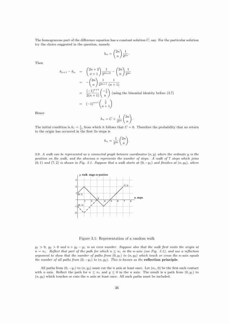
3.9. A walk can be represented as a connected graph between coordinates (n, y) where the ordinate y is theposition on the walk, and the abscissa n represents the number of steps. A walk of 7 steps which joins(0, 1) and (7, 2) is shown in Fig. 3.1. Suppose that a walk starts at (0,−y1) and finishes at (n, y2), where
Figure 3.1: Representation of a random walk
y1 > 0, y2 > 0 and n + y2 − y1 is an even number. Suppose also that the walk first visits the origin atn = n1. Reflect that part of the path for which n ≤ n1 in the n-axis (see Fig. 3.1), and use a reflectionargument to show that the number of paths from (0, y1) to (n, y2) which touch or cross the n-axis equalsthe number of all paths from (0,−y1) to (n, y2). This is known as the reflection principle.
All paths from (0,−y1) to (n, y2) must cut the n axis at least once. Let (n1, 0) be the first such contactwith n axis. Reflect the path for n ≤ n1 and y ≤ 0 in the n axis. The result is a path from (0, y1) to(n, y2) which touches or cuts the n axis at least once. All such paths must be included.
36
3.10. A walk starts at (0, 1) and returns to (2n, 1) after 2n steps. Using the reflection principle (see Problem3.9) show that there are
(2n)!
n!(n + 1)!
different paths between the two points which do not ever revisit the origin. What is the probability thatthe walk ends at (2n, 1) after 2n steps without ever visiting the origin, assuming that the random walk issymmetric?
Show that the probability that the first visit to the origin after 2n+1 steps is
pn =1
22n+1
(2n)!
n!(n + 1)!.
Let M(m, d) represent the total number of different paths in the (n, y) plane which are of length mjoining positions denoted by y = y1 and y = y2: here d is the absolute difference d = |y2 − y1|. The totalnumber of paths from (0, 1) to (0, 2n) is
M(2n, 0) =
(2n
n
).
By the reflection principle (Problem 3.9) the number of paths which cross the n axis (that is, visit theorigin) is
M(2n, 2) =
(2n
n− 1
).
Hence the number of paths from (0, 1) to (0, 2n) which do not visit the origin is
M(2n, 0)−M(2n, 2) =
(2n
n
)−
(2n
n− 1
)=
(2n)!
n!n!− (2n)!
(n− 1)!(n + 1)!
=(2n)!)
n!(n + 1)!
The total number of paths is 22n. Also to visit the origin for the first time at step 2n + 1, the walkmust be at y = 1 at step 2n, from where there is a probability of 1
2that the walk moves to the origin.
Hence the probability is
pn =1
22n
(2n)!
n!(n + 1)!
1
2=
1
22n+1
(2n)!
n!(n + 1)!.
3.11. A symmetric random walks starts at the origin. Let fn,1 be the probability that the first visit toposition x = 1 occurs at the n-th step. Obviously, f2n,1 = 0. The result from Problem 3.10 can be adaptedto give
f2n+1,1 =1
22n+1
(2n)!
n!(n + 1)!, (n = 0, 1, 2, . . .).
Suppose that its pgf is
G1(s) =
∞∑n=0
f2n+1,1s2n+1.
Show thatG1(s) = [1− (1− s2)
12 ]/s.
[Hint: the identity
1
22n+1
(2n)!
n!(n + 1)!= (−1)n
(12
n + 1
), (n = 0, 1, 2, . . .)
is useful in the derivation of G1(s).]Show that any walk starting at the origin is certain to visit x > 0 at some future step, but that the
mean number of steps in achieving this is infinite.
37
The result
f2n+1,1 =1
22n+1
(2n)!
n!(n + 1)!
is simply the result in the last part of Problem 3.10.For the pgf
G1(s) =
∞∑n=0
f2n+1,1s2n+1 =
∞∑n=0
1
22n+1
(2n)!s2n+1
n!(n + 1)!
The identity before (3.7) (in the book) states that(
2n
n
)= (−1)n
(− 1
2
n
)22n.
Therefore, using this result
(2n)!
22n+1n!(n + 1)!=
(2n
n
)1
22n+1(n + 1)= (−1)n
(− 1
2
n
)1
2(n + 1)= (−1)n
(12
n + 1
).
Hence
G1(s) =
∞∑s=0
(−1)n
(12
n + 1
)s2n+1
=
(12
1
)s−
(12
2
)s3 +
(12
3
)s5 − · · ·
=1
s[1− (1− s2)
12 ]
using the binomial theorem.That G1(1) = 1 implies that the random walk is certain to visit x > 0 at some future step. However,
G′(1) = ∞ which means that expected number to that event is infinite.
3.12. A symmetric random walk starts at the origin. Let fn,x be the probability that the first visit to positionx occurs at the n-th step (as usual, fn,x = 0 if n + x is an odd number). Explain why
fn,x =
n−1∑k=1
fn−k,x−1fk,1, (n ≥ x > 1).
If Gx(s) is its pgf, deduce thatGx(s) = {G1(s)}x,
where G1(s) is given explicitly in Problem 3.11. What are the probabilities that the walk first visits x = 3at the steps n = 3, n = 5 and n = 7?
Consider k = 1. The first visit to x− 1 has probability fn−1,x−1 in n− 1 steps. Having reached therethe walk must first visit x in one further step with probability f1,1. Hence the probability is fn−1,x−1f1,1.If k = 2, the first visit to x − 1 in n − 2 steps occurs with probability fn−2,x−1: its first visit to x mustoccur after two steps. Hence the probability is fn−2,x−1f2,1. And so on. The sum of these probabilitiesgives
fn,x =
n−1∑k=1
fn−k,x−1fk,1, (n ≥ x > 1).
Multiply both sides of this equation by sn and sum over n from n = x:
Gx(s) =
∞∑n=x
n−1∑k=1
fn−k,x−1fk,1sn = Gx−1(s)G1(s).
By repeated application of this difference equation, it follows that
Gx(s) =[1
s
{1− (1− s2)
12
}]x
.
38
For x = 3,
G1(s) =[1
s
{1− (1− s2)
12
}]3
.
Expansion of this function as a Taylor series in s gives the coefficients and probabilities:
G2(s) =1
4s3 +
1
8s5 +
1
64s7 + O(s9).
3.13. Problem 3.12 looks at the probability of a first visit to position x ≥ 1 at the n-th step in a symmetricrandom walk which starts at the origin. Why is the pgf for the first visit to position x where |x| ≥ 1 givenby
Gx(s) = {G1(s)}|x|,where F1(s) is defined in Problem 3.11?
First visits to x > 0 and to −x at step n must be equally likely. Hence fn,x = fn,−x. Therefore
Gx(s) = [1− (1− s2)12 ]|x|.
3.14. An asymmetric walk has parameters p and q = 1−p 6= p. Let gn,1 be the probability that the first visitto x = 1 occurs at the n-th step. As in Problem 3.11, g2n,1 = 0. It was effectively shown in Problem 3.10that the number of paths from the origin, which return to the origin after 2n steps is
(2n)!
n!(n + 1)!.
Explain why
g2n+1,1 =(2n)!
n!(n + 1)!pn+1qn.
Suppose that its pgf is
G1(s) =
∞∑n=0
g2n+1,1s2n+1.
Show thatG1(s) = [1− (1− 4pqs2)
12 ]/(2qs).
(The identity in Problem 3.11 is required again.)What is the probability that the walk ever visits x > 0? How does this result compare with that for the
symmetic random walk?What is the pgf for the distribution of first visits of the walk to x = −1 at step 2n + 1?
The probability that the first return to x = 1 at the (2n + 1)th step is g2n+1,1 The number of paths oflength 2n which never visit x = 1 is (adapt the answer in Problem 3.10),
(2n)!
n!(n + 1)!.
The consequent probability of this occurrence is, since there are n steps to the right with probability pand to the left with probability q,
(2n)!
n!(n + 1)!pnqn.
the probability that the next step visits x = 1 is
(2n)!
n!(n + 1)!pn+1qn,
which is the previous probability multiplied by p. Using the identity in Problem 3.11,
g2n+1,1 =
(12
n + 1
)(−1)n(2p)n(2q)n2p.
39
Its pgf G1(s) is given by
G1(s) =
∞∑n=0
(12
n + 1
)(−1)n(4pq)n2ps2n+1 = [1− (1− 4pqs2)
12 ]/(2qs)
using a binomial expansion.Use an argumant that any walk which enters x > 0 must first visit x = 1 as follows. The probability
that the walks first visit to x = 1 occurs at all is
∞∑n=0
g2n+1,1 = G1(1) =1
2q[1− {(p + q)2 − 4pq} 1
2 ] =1
2q[1− |p− q|].
A symmetry argument in which p and q are interchanged gives the pgf for the distribution of first visitsto x = −1, namely
H1(s) = [1− (1− 4pqs2)12 ]/(2ps).
3.15. It was shown in Section 3.3 that, in a random walk with parameters p and q = 1− p, the probabilitythat a walk is at position x at step n is given by
vn,x =
(n
12(n + x)
)p
12 (n+x)q
12 (n−x), |x| ≤ n,
where 12(n + x) must be an integer. Verify that vn,x satisfies the difference equation
vn+1,x = pvn,x−1 + qvn,x+1,
subject to the initial conditionsv0,0 = 1, vn,x = 0, (x 6= 0).
Note that this difference equation has differences on two arguments.Can you develop a direct argument which justifies the difference equation for the random walk?
Given
vn,x =
(n
12(n + x)
)p
12 (n+x)q
12 (n−x), |x| ≤ n,
then
pvn,x−1 + qvn,x+1 = p
(n
12(n + x− 1)
)p
12 (n+x−1)q
12 (n−x+1)
+q
(n
12(n + x + 1)
)p
12 (n+x+1)q
12 (n−x−1)
= p12 (n+x+1)q
12 (n−x+1)
[(n
12(n + x− 1)
)+
(n
12(n + x + 1)
)]
=p
12 (n+x+1)q
12 (n−x+1)n!
[ 12(n + x + 1)]![ 1
2(n− x + 1)]!
[ 12(n + x + 1) + 1
2(n− x + 1)]
= p12 (n+x+1)q
12 (n−x+1)
(n + 1
12(n + x)
)= vn+1,x.
3.16. In the usual notation, v2n,0 is the probability that, in a symmetric random walk, the walk visits theorigin after 2n steps. Using the difference equation from Problem 3.15, v2n,0 satisfies
v2n,0 = 12v2n−1,−1 + 1
2v2n−1,1 = v2n−1,1.
How can the last step be justified? Let
G1(s) =
∞∑n=1
v2n−1,1s2n−1
40
be the pgf of the distribution {v2n−1,1}. Show that
G1(s) = [(1− s2)−12 − 1]/s.
By expanding G1(s) as a power series in s show that
v2n−1,1 =
(2n− 1
n
)1
22n−1.
By a repetition of the argument show that
G2(s) =
∞∑n=0
v2n,2s2n = [(2− s)(1− s2)−
12 − 2]/s.
Use a symmetry argument. Multiply both sides of the difference equation by s2n and sum from n = 1to infinity. Then
∞∑n=1
v2n,0s2n = s
∞∑n=1
v2n−1,1s2n−1.
Therefore in the notation in the problem
H(s)− 1 = sG1(s),
where H(s) = (1− s2)12 . Therefore
G1(s) =
∞∑n=1
v2n−1,1s2n−1
as required.From the series for G1(s) expanded as a binomial series, the general coefficient is
v2n−1,1 =
(− 1
2
n
)(−1)n =
(2n
n
)1
22n=
(2n)!
22nn!n!=
(2n− 1
n
)1
22n−1.
From the difference equationv2n+1,1 = 1
2v2n,0 + 1
2v2n,2.
Multiplying by s2n+1 and summing over n
G1(s) =1
2
∞∑n=0
v2n,0s2n+1 +
1
2
∞∑n=0
v2n,2s2n+1 =
1
2sH(s) +
1
2sG2(s).
Therefore
G2(s) =1
3[(2− s)(1− s2)−
12 − 2].
3.17. A random walk takes place on a circle which is marked out with n positions. Thus, as shown inFig. 3.2, position n is the same as position O. This is known as a cyclic random walk of period n. Asymmetric random walk starts at O. What is the probability that the walk is at O after j steps in the cases:(a) j < n;(b) n ≤ j < 2n?Distinguish carefully the cases in which j and n are even and odd.
(a) j < n. The walk cannot circumscribe the circle. This case is the same as the walk on a line. Letpj be the probability that the walk is at O at step j. Then by (3.6)
pn = vn,0 =
(n12n
)1
2nn even
0 n odd
41
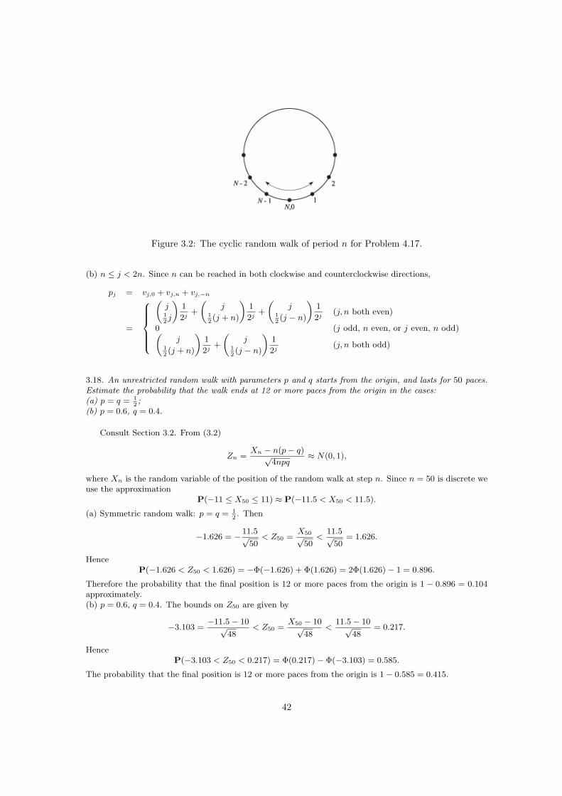
Figure 3.2: The cyclic random walk of period n for Problem 4.17.
(b) n ≤ j < 2n. Since n can be reached in both clockwise and counterclockwise directions,
pj = vj,0 + vj,n + vj,−n
=
(j12j
)1
2j+
(j
12(j + n)
)1
2j+
(j
12(j − n)
)1
2j(j, n both even)
0 (j odd, n even, or j even, n odd)(j
12(j + n)
)1
2j+
(j
12(j − n)
)1
2j(j, n both odd)
3.18. An unrestricted random walk with parameters p and q starts from the origin, and lasts for 50 paces.Estimate the probability that the walk ends at 12 or more paces from the origin in the cases:(a) p = q = 1
2;
(b) p = 0.6, q = 0.4.
Consult Section 3.2. From (3.2)
Zn =Xn − n(p− q)√
4npq≈ N(0, 1),
where Xn is the random variable of the position of the random walk at step n. Since n = 50 is discrete weuse the approximation
P(−11 ≤ X50 ≤ 11) ≈ P(−11.5 < X50 < 11.5).
(a) Symmetric random walk: p = q = 12. Then
−1.626 = − 11.5√50
< Z50 =X50√
50<
11.5√50
= 1.626.
HenceP(−1.626 < Z50 < 1.626) = −Φ(−1.626) + Φ(1.626) = 2Φ(1.626)− 1 = 0.896.
Therefore the probability that the final position is 12 or more paces from the origin is 1 − 0.896 = 0.104approximately.(b) p = 0.6, q = 0.4. The bounds on Z50 are given by
−3.103 =−11.5− 10√
48< Z50 =
X50 − 10√48
<11.5− 10√
48= 0.217.
HenceP(−3.103 < Z50 < 0.217) = Φ(0.217)− Φ(−3.103) = 0.585.
The probability that the final position is 12 or more paces from the origin is 1 − 0.585 = 0.415.
42
3.19. In an unrestricted random walk with parameters p and q, for what value of p are the mean andvariance of the probability distribution of the position of the walk at stage n the same?
From Section 3.2 the mean and variance of Xn, the random variable of the position of the walk at stepn, are given by
E(Xn) = n(p− q), V(Xn) = 4npq,
where q = 1− p. The mean and variance are equal if 2p− 1 = 4p(1− p), that is, if
4p2 − 2p− 1 = 0.
The required probability is p = 14(1 +
√5).
3.20. Two walkers each perform symmetric random walks with synchronized steps both starting from theorigin at the same time. What is the probability that they are both at the origin at step n?
If A and B are the walkers, then the probability an that A is at the origin is given by
an =
(n12n
)1
2n(n even)
0 (n odd)
.
The probability bn for B is given by the same formula. They can only visit the origin if n is even, in whichcase the probability that they are both there is
anbn =
(n12n
)21
22n.
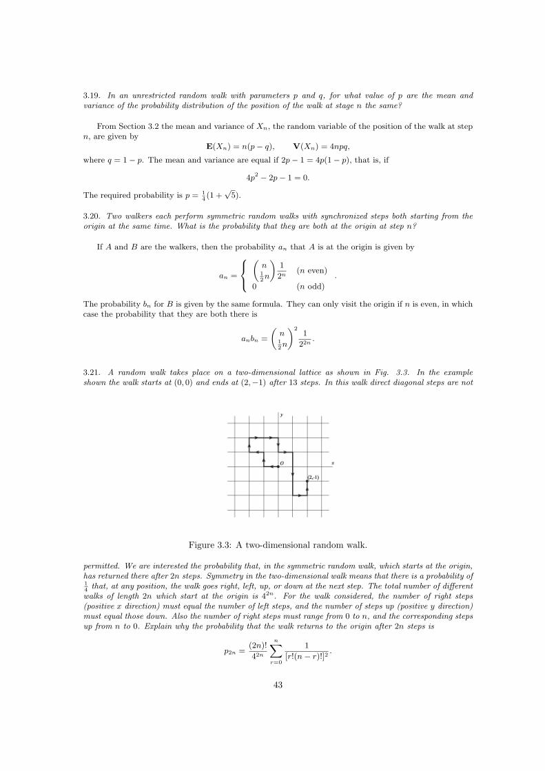
3.21. A random walk takes place on a two-dimensional lattice as shown in Fig. 3.3. In the exampleshown the walk starts at (0, 0) and ends at (2,−1) after 13 steps. In this walk direct diagonal steps are not
Figure 3.3: A two-dimensional random walk.
permitted. We are interested the probability that, in the symmetric random walk, which starts at the origin,has returned there after 2n steps. Symmetry in the two-dimensional walk means that there is a probability of14
that, at any position, the walk goes right, left, up, or down at the next step. The total number of differentwalks of length 2n which start at the origin is 42n. For the walk considered, the number of right steps(positive x direction) must equal the number of left steps, and the number of steps up (positive y direction)must equal those down. Also the number of right steps must range from 0 to n, and the corresponding stepsup from n to 0. Explain why the probability that the walk returns to the origin after 2n steps is
p2n =(2n)!
42n
n∑r=0
1
[r!(n− r)!]2.
43
Prove the two identities
(2n)!
[r!(n− r)!]2=
(2n
n
)(n
r
)2
,
(2n
n
)=
n∑r=0
(n
r
)2
.
[Hint: compare the coefficients of xn in (1 + x)2n and [(1 + x)n]2.] Hence show that
p2n =1
42n
(2n
n
)2
.
Calculate p2, p4, 1/(πp40), 1/(πp80). How do you would you guess that p2n behaves for large n?
At each intersection there are 4 possible paths. Hence there are 42n different paths which start theorigin.
For a walk which returns to the origin there must be r, say, left and right steps, and n−r up and downsteps (r = 0, 1, 2, . . . , n) to ensure the return. For fixed r, the number of ways in which r left, r right,(n− r) up and (n− r) down steps can be chosen from 2n is the multinomial formula
(2n)!
r!r!(n− r)!(n− r)!.
For all r, the total number of ways is
n∑r=0
(2n)!
r!r!(n− r)!(n− r)!.
Therefore the probability that a return to the origin occurs is
p2n =(2n)!
42n
n∑r=0
1
[r!(n− r)!]2.
For example if n = 2, then
p4 =4!
44
2∑r=0
1
r!(2− r)!=
4!
44
(1
2+ 1 +
1
2
)=
3
16.
For the first identity
(2n)!
[r!(n− r)!]2=
(2n)!
n!n!
(n!
r!(n− r)!
)2
=
(2n
n
)(n
r
)2
.
For the second identity
(2n
n
)= the coefficient of xn in the expansion of (1 + x)2n
= the coefficient of xn in the expansion of [(1 + x)n]2
= the coefficient of xn in
[1 +
(n
1
)x +
(n
2
)x2 + · · ·+
(n
n
)xn
]2
=
(n
0
)(n
n
)+
(n
1
)(n
n− 1
)+ · · · +
(n
n
)(n
0
)
=
(n
0
)2
+
(n
1
)2
+ · · ·(
n
n
)2 [since
(n
r
)=
(n
n− r
)]
=
n∑r=0
(n
r
)2
44
Hence
p2n =2
42n
(2n
n
)2
.
The computed values are p20 = 0.01572 and p40 = 0.00791. Then
1
πp20= 20.25,
1
πp40= 40.25,
which imply that possibly p2n ∼ 1/(nπ) as n →∞.
3.22. A random walk takes place on the positions {. . . ,−2,−1, 0, 1, 2, . . .}. The walk starts at 0. At stepn, the walker has a probability qn of advancing one position, or a probability 1− qn of retreating one step(note that the probability depends on the step not the position of the walker). Find the expected position ofthe walker at step n. Show that if qn = 1
2+ rn, (− 1
2< rn < 1
2), and the series
∑∞j=1
rj is convergent, thenthe expected position of the walk will remain finite as n →∞.
If Xn is the random variable representing the position of the walker at step n, then
P(Xn+1 = j + 1|Xn = j) = qn, P(Xn+1 = j − 1|Xn = j) = 1− qn.
If Wi is the modified Bernoulli random variable (Section 3.2), then
E(Xn) = E
n∑i=1
Wi =
n∑i=1
E(Wi) =
n∑i=1
[1.qi + (−1)(1− qi)]
= 2
n∑i=1
qi − n.
Let qn = 12
+ rn, (− 12
< rn < 12). Then
E(Xn) = 2
n∑i=1
( 12
+ ri)− n =
n∑i=1
ri.
Hence E(Xn) is finite as n →∞ if the series on the right is convergent.
3.23. A symmetric random walk starts at k on the positions 0, 1, 2, . . . , a, where 0 < k < a. As,in thegambler’s ruin problem, the walk stops whenever 0 or a is first reached. Show that the expected number ofvisits to position j where 0 < j < k is 2j(a− k)/a before the walk stops.
One approach is to this problem by repeated application of result (2.5) for gamnler’s ruin.A walk which starts at k first reached j before a with probability (by (2.5))
p =(a− j)− (k − j)
a− j=
a− k
a− j.
A walk which starts at j reaches a (and stops) before reaching j (again by (2.5)) with probability
1
2
1
a− j=
1
2(a− j),
and reaches 0 before returning to j with probability
j − (j − 1)
2j=
1
2j.
Hence the probability that the walk from j stops without returning to j with probability
q =1
2(a− j)+
1
2j=
a
2j(a− j).
45
Given that the walk is at j, it nexts visits j with probability
r = 1− q = 1− a
2j(a− j)=
2j(a− j)− a
2j(a− j).
Therefore the probability that the walk starts from k visits j m times before stopping is
hm = prm−1q.
The expected number of visits to j is
µ =
∞∑m=1
mhm = pq
∞∑m=1
mrm−1 =pq
(1− r)2,
summing the quasi-geometric series. Substituting for p, q, and r,
µ =a− k
a− j· a
2j(a− j)
[1− 2j(a− j)− a
2j(a− j)
]−2
=a(a− k)
2j(a− j)2· 4j2(a− j)2
a2=
2(a− k)j
a
46
Chapter 4
Markov chains
4.1. If T = [pij ], (i, j = 1, 2, 3) and
pij =i + j
6 + 3i,
show that T is a row-stochastic matrix. What is the probability that a transition between states E2 and E3
occurs at any step?If the initial probability distribution in a Markov chain is
p(0) =[
12
14
14
],
what are the probabilities that states E1, E2 and E3 are occupied after one step. Explain why the probabilitythat the chain finishes in state E2 is 1
3irrespective of the number of steps.
Since
pij =i + j
6 + 3i,
then3∑
j=1
pij =
3∑j=1
i + j
6 + 3i=
3i
6 + 3i+
6
6 + 3i= 1,
for all i. Also 0 < pi,j < 1. Therefore T is a stochastic matrix. The probability that a transition from E2
to E3 occurs is p23 = 512
.
The probabilities that the states E1, E2 and E3 are occupied after one step given p(0) are given by
p(1) = p(0)T =[
12
14
14
]
29
13
49
14
13
512
415
13
25
=
[173720
13
307720
]
Each term in the second column of T is a 13. By row-on-column matrix multiplication, each element
in the second column of T n is a 13. Hence the second term in p(0)T
n is 13
independently of p(0).
4.2. If
T =
12
14
14
13
13
13
14
12
14
,
calculate p(2)22 , p
(2)31 and p
(2)13 .
p(2)ij are the elements of T 2. The matrix multiplication gives
T 2 =
1948
13
1348
1336
1336
518
1748
1748
724
.
47
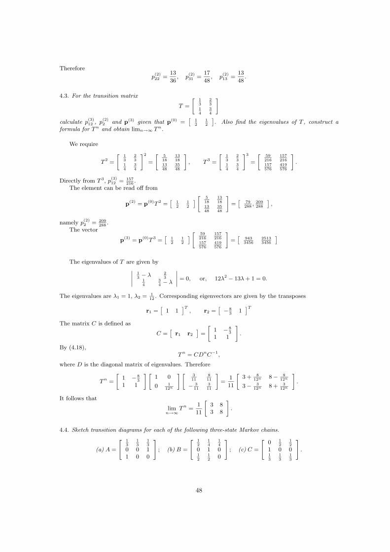
Therefore
p(2)22 =
13
36, p
(2)31 =
17
48, p
(2)13 =
13
48.
4.3. For the transition matrix
T =
[13
23
14
34
]
calculate p(3)12 , p
(2)2 and p(3) given that p(0) =
[12
12
]. Also find the eigenvalues of T , construct a
formula for T n and obtain limn→∞ T n.
We require
T 2 =
[13
23
14
34
]2
=
[518
1318
1348
3548
], T 3 =
[13
23
14
34
]3
=
[59216
157216
157576
419576
].
Directly from T 3, p(3)12 = 157
216.
The element can be read off from
p(2) = p(0)T 2 =[
12
12
] [518
1318
1348
3548
]=
[79288
, 209288
],
namely p(2)2 = 209
288.
The vector
p(3) = p(0)T 3 =[
12
12
] [59216
157216
157576
419576
]=
[9433456
25133456
]
The eigenvalues of T are given by
∣∣∣∣13− λ 2
314
34− λ
∣∣∣∣ = 0, or, 12λ2 − 13λ + 1 = 0.
The eigenvalues are λ1 = 1, λ2 = 112
. Corresponding eigenvectors are given by the transposes
r1 =[
1 1]T
, r2 =[− 8
31
]T
The matrix C is defined as
C =[
r1 r2
]=
[1 − 8
3
1 1
].
By (4.18),T n = CDnC−1,
where D is the diagonal matrix of eigenvalues. Therefore
T n =
[1 − 8
3
1 1
][1 0
0 112n
][311
811
− 311
311
]=
1
11
[3 + 8
12n 8− 812n
3− 312n 8 + 3
12n
].
It follows that
limn→∞
T n =1
11
[3 83 8
].
4.4. Sketch transition diagrams for each of the following three-state Markov chains.
(a) A =
[ 13
13
13
0 0 11 0 0
]; (b) B =
[ 12
14
14
0 1 012
12
0
]; (c) C =
[0 1
212
1 0 013
13
13
].
48
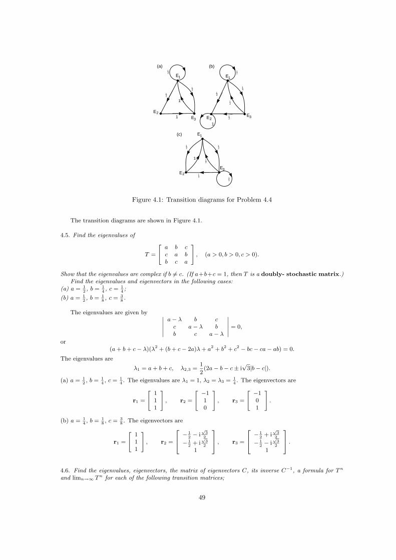
E1 E1
E1
E2E2
E2
E3E3
E3
12
12
12
12
12
12
12
12
13
13
13
14
14
1
1
1
1
(a) (b)
(c)
Figure 4.1: Transition diagrams for Problem 4.4
The transition diagrams are shown in Figure 4.1.
4.5. Find the eigenvalues of
T =
[a b cc a bb c a
], (a > 0, b > 0, c > 0).
Show that the eigenvalues are complex if b 6= c. (If a+b+c = 1, then T is a doubly- stochastic matrix.)Find the eigenvalues and eigenvectors in the following cases:
(a) a = 12, b = 1
4, c = 1
4;
(b) a = 12, b = 1
8, c = 3
8.
The eigenvalues are given by ∣∣∣∣∣a− λ b c
c a− λ bb c a− λ
∣∣∣∣∣ = 0,
or(a + b + c− λ)(λ2 + (b + c− 2a)λ + a2 + b2 + c2 − bc− ca− ab) = 0.
The eigenvalues are
λ1 = a + b + c, λ2,3 =1
2(2a− b− c± i
√3|b− c|).
(a) a = 12, b = 1
4, c = 1
4. The eigenvalues are λ1 = 1, λ2 = λ3 = 1
4. The eigenvectors are
r1 =
[111
], r2 =
[ −110
], r3 =
[ −101
].
(b) a = 14, b = 1
8, c = 3
8. The eigenvectors are
r1 =
[111
], r2 =
− 1
2− i
√3
2
− 12
+ i√
32
1
, r3 =
− 1
2+ i
√3
2
− 12− i
√3
2
1
.
4.6. Find the eigenvalues, eigenvectors, the matrix of eigenvectors C, its inverse C−1, a formula for T n
and limn→∞ T n for each of the following transition matrices;
49
(a)
T =
[18
78
12
12
];
(b)
T =
[ 12
18
38
14
38
38
14
58
18
];
(a) The eigenvalues are λ1 = 1, λ2 = − 38. The corresponding eigenvectors are
r1 =
[11
], r2 =
[− 7
4
1
].
The matrix C and its inverse are given by
C =[
r1 r2
]=
[1 − 7
4
1 1
], C−1 =
[ 411
711
− 411
411
].
The matrix T n is given by
T n = CDnC−1 =
[1 − 7
4
1 1
][1 00 − 3
8
]n [ 411
711
− 411
411
]
=1
11
[4 + 7(− 3
8)n 7− 7(− 3
8)n
4− (− 38)n 7 + (− 3
8)n
]→ 1
11
[4 7
4 7
]
as n →∞.(b) The eigenvalues are λ1 = − 1
4, λ2 = 1
4, λ3 = 1, and the corresponding eigenvectors are
r1 =
− 3
7
− 37
1
, r2 =
[ −211
], r3 =
[111
]
The matrix C is given by
C =[
r1 r2 r3
]=
− 3
7−2 1
− 37
1 1
1 1 1
Then
T n = CDnC−1 =
− 3
7−2 1
− 37
1 1
1 1 1
[(− 1
4)n 0 0
0 ( 14)n 0
0 0 1
]
0 − 710
710
− 13
13
113
1130
310
=
13
+ 1321−2n 11
30+ 3
5(−1)n2−1−2n − 1
321−2n 3
10− 3
5(−1)n2−1−2n
13− 4n
31130
+ 35(−1)n2−1−2n + 4−n
3310− 3
5(−1)n2−1−2n
13− 4−n
31130− 7
5(−1)n2−1−2n + 4−n
3310
+ 75(−1)n2−1−2n
,
so that
limt→∞
T n =
13
1130
310
13
1130
310
13
1130
310
.
4.7. The weather in a certain region can be characterized as being sunny(S), cloudy(C) or rainy(R) onany particular day. The probability of any type of weather on one day depends only on the state of the
50
weather on the previous day. For example, if it is sunny one day then sun or clouds are equally likely onthe next day with no possibility of rain. Explain what other the day-to-day possibilities are if the weatheris represented by the transition matrix.
T =
S C R
S 12
12
0C 1
214
14
R 0 12
12
Find the eigenvalues of T and a formula for T n. In the long run what percentage of the days are sunny,cloudy and rainy?
The eigenvalues of T are given by
∣∣∣∣∣
12− λ 1
20
12
14− λ 1
4
0 12
12− λ
∣∣∣∣∣ = −1
8(4λ + 1)(2λ− 1)(λ− 1) = 0.
Let λ1 = − 14, λ2 = 1
2and λ3 = 1. The coresponding eigenvectors are
r1 =
1
− 32
1
, r2 =
[ − 12
01
], r3 =
[111
]
The matrix of eigenvectors C is given by
C =[
r1 r2 r3
]=
1 − 12
1
− 32
0 1
1 1 1
If D is the diagonal matrix of eigenvalues, then by (4.18)
T n = CDnC−1 =
1 − 12
1
− 32
0 1
1 1 1
[(− 1
4)n 0 0
0 ( 12)n 0
0 0 1
]
415
− 25
215
− 23
0 23
25
25
15
As n →∞
T n →
1 − 12
1
− 32
0 1
1 1 1
[0 0 00 0 00 0 1
]
415
− 25
215
− 23
0 23
25
25
15
=
1
5
[2 2 12 2 12 2 1
].
In the long run 40% of the days are of the days are sunny, 40% are cloudy and 20% are rainy.
4.8. The eigenvalue method of Section 4.4 for finding general powers of stochastic matrices is only guaran-teed to work if the eigenvalues are distinct. Several possibilities occur if the stochastic matrix of a Markovchain has a repeated eigenvalue. The following three examples illustrate these possibilities.(a) Let
T =
[ 14
14
12
1 0 012
14
14
]
be the transition matrix of a three-state Markov chain. Show that T has the repeated eigenvalue λ1 = λ2 =− 1
4and λ3 = 1, and two distinct eigenvectors
r1 =
[1−41
]r3 =
[111
].
51
In this case diagonalization of T is not possible. However it is possible to find a non-singular matrix Csuch that
T = CJC−1,
where J is the Jordan decomposition matrix given by
J =
[λ1 1 00 λ1 00 0 1
]=
[ − 14
1 00 − 1
40
0 0 1
],
C =[
r1 r2 r3
],
and r2 satisfies(T − λ1I3)r2 = r1.
Show that we can choose
r2 =
[ −10240
].
Find a formula for Jn and confirm that, as n →∞,
T n →
1225
15
825
1225
15
825
1225
15
825
.
(b) A four-state Markov chain has the transition matrix
S =
1 0 0 034
0 14
00 1
40 3
4
0 0 0 1
.
Sketch the transition diagram for the chain, and note that the chain has two absorbing states and is thereforenot a regular chain. Show that the eigenvalues of S are − 1
4, 1
4and 1 repeated. Show that there are four
distinct eigenvectors. Choose the diagonalizing matrix C as
C =
0 0 −4 −5−1 1 −3 41 1 0 10 0 1 0
.
Find its inverse, and show that, as n →∞,
Sn →
1 0 0 045
0 0 15
15
0 0 45
0 0 0 1
.
Note that since the rows are not the same this chain does not have an invariant distribution: this is causedby the presence of two absorbing states.(c) Show that the transition matrix
U =
[ 12
0 12
16
13
12
16
0 56
]
has a repeated eigenvalue, but that, in this case, three independent eigenvectors can be associated with U .Find a diagonalizing matrix C, and find a formula for Un using Un = CDnC−1, where
D =
[ 13
0 00 1
30
0 0 1
].
52
Confirm also that this chain has an invariant distribution.
(a) The eigenvalues are given by
∣∣∣∣∣
14− λ 1
412
1 −λ 012
14
14− λ
∣∣∣∣∣ = − 1
16(λ− 1)(1 + 4λ)2
Hence they are λ1 = − 14
(repeated) and λ2 = 1. This leads to the two eigenvectors
r1 =
[1−41
], r3 =
[111
]
The Jordan decomposition matrix is given by
J =
[ − 14
1 00 − 1
40
0 0 1
].
Let r2 satisfy
[T − λ1I3]r2 = r1 or
12
14
12
1 14
012
14
12
r2 =
1
−4
1
.
The solution for the linear equations for the components of r2 gives
r2 =[−10 24 0
]T.
The matrix C is defined in the usual way as
C =[
r1 r2 r3
]=
[1 −10 1−4 24 11 0 1
].
Its computed inverse is
C−1 =
− 12
25− 1
51725
− 110
0 110
1225
15
825
.
If T = CJC−1, then T n = CJnC−1, where
Jn =
− 1
41 0
0 − 14
0
0 0 1
n
=
(− 14)n n(− 1
4)n−1 0
0 (− 14)n 0
0 0 1
.
As n →∞,
T n →
1 −10 1
−4 24 1
1 0 1
0 0 0
0 0 0
0 0 1
− 12
25− 1
51725
− 110
0 110
1225
15
825
=
1225
15
825
1225
15
825
1225
15
825
.
(b) The transition diagram is shown in Figure 4.2. The eigenvectors are given by
∣∣∣∣∣∣∣
1− λ 0 0 034
−λ 14
00 1
4−λ 3
4
0 0 0 1− λ
∣∣∣∣∣∣∣=
1
16(λ− 1)2(4λ− 1)(4λ + 1) = 0.
53
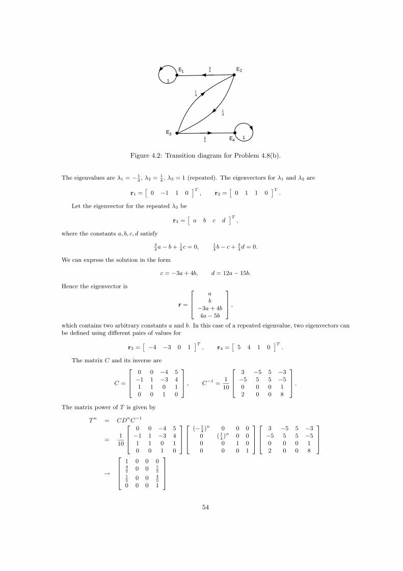
E1 E2
E3
1
1E434
34
14
14
Figure 4.2: Transition diagram for Problem 4.8(b).
The eigenvalues are λ1 = − 14, λ2 = 1
4, λ3 = 1 (repeated). The eigenvectors for λ1 and λ2 are
r1 =[
0 −1 1 0]T
, r2 =[
0 1 1 0]T
.
Let the eigenvector for the repeated λ3 be
r3 =[
a b c d]T
,
where the constants a, b, c, d satisfy
34a− b + 1
4c = 0, 1
4b− c + 3
4d = 0.
We can express the solution in the form
c = −3a + 4b, d = 12a− 15b.
Hence the eigenvector is
r =
ab
−3a + 4b4a− 5b
,
which contains two arbitrary constants a and b. In this case of a repeated eigenvalue, two eigenvectors canbe defined using different pairs of values for
r3 =[−4 −3 0 1
]T, r4 =
[5 4 1 0
]T.
The matrix C and its inverse are
C =
0 0 −4 5−1 1 −3 41 1 0 10 0 1 0
, C−1 =
1
10
3 −5 5 −3−5 5 5 −50 0 0 12 0 0 8
.
The matrix power of T is given by
T n = CDnC−1
=1
10
0 0 −4 5−1 1 −3 41 1 0 10 0 1 0
(− 14)n 0 0 0
0 ( 14)n 0 0
0 0 1 00 0 0 1
3 −5 5 −3−5 5 5 −50 0 0 12 0 0 8
→
1 0 0 045
0 0 15
15
0 0 45
0 0 0 1
54
as n →∞(c) The eigenvaues are given by
∣∣∣∣∣
12− λ 0 1
216
13− λ 1
216
0 56− λ
∣∣∣∣∣ = −1
9(λ− 1)(3λ− 1)2.
Hence the eigenvalues are λ1 = 13
(repeated) and λ3 = 1. Corresponding to the eigenvalue λ1, we canobtain the eigenvector
r1 =
[ −3bab
]= b
[ −301
]+ a
[010
],
where a and b are arbitrary. Two distinct eigenvectors can be obtained by putting a = 0, b = 1 and byputting a = 1, b = 0. The three eigenvectors are
r1 =
[ −301
], r2 =
[010
], r3 =
[111
].
The matrix C and its inverse become
C =
[ −3 0 10 1 11 0 1
], C−1 =
1
4
[ −1 0 1−1 4 −31 0 3
].
With
D =
[ 13
0 00 1
30
0 0 1
],
then
Un =
[ −3 0 10 1 11 0 1
][( 13)n 0 00 ( 1
3)n 0
0 0 1
]1
4
[ −1 0 1−1 4 −31 0 3
]
→[ −3 0 1
0 1 11 0 1
][0 0 00 0 00 0 1
]1
4
[ −1 0 1−1 4 −31 0 3
]
=
14
0 34
14
0 34
14
0 34
,
as n →∞.
4.9. Miscellaneous problems on transition matrices. In each case find the eigenvalues of T , a formula forT n and the limit of T n as n →∞. The special cases discussed in Problem 4.8 can occur.(a)
T =
[ 12
732
932
1 0 012
14
14
];
(b)
T =
[ 13
14
512
1 0 014
14
12
];
(c)
T =
[ 14
316
916
34
0 14
14
14
12
];
55
(d)
T =
[ 14
14
12
512
13
14
12
14
14
];
(e)
T =
1 0 0 012
0 0 12
0 0 1 00 1
212
0
.
(a) The eigenvalues of T are λ1 = − 18
(repeated) and λ3 = 1, with the corresponding eigenvectors
r1 =
[ 14
−21
], r2 =
[111
].
The Jordan decomposition matrix J is required, where
J =
[ − 18
1 00 − 1
80
0 0 1
],
and r2 is given by
[T − λ1I3]r2 = r1 or
58
732
932
1 18
012
14
38
r2 =
14
−2
1
The remaining eigenvector is
r2 =
[ −3843
].
The matrix C and its inverse are given by
C =
14
−3 1
−2 8 1
1 43
1
, C−1 =
− 10
27− 13
541118
− 16
124
18
1627
527
29
Then
T n =
14
−3 1
−2 8 1
1 43
1
(− 18)n 1 0
0 (− 18)n 0
0 0 1
− 10
27− 13
541118
− 16
124
18
1627
527
29
Matrix multiplcation gives
limn→∞
T n =
1627
527
29
1627
527
29
1627
527
29
.
(b) The eigenvalues of T are λ1 = − 14, λ2 = − 1
6, and λ3 = 1, which are all different, so that the
calculations are straightforward. The eigenvectors are given by
r1 =
1
−4
1
, r2 =
512
− 52
1
, r3 =
1
1
1
The matrix C and its inverse are
C =
1 512
1
−4 − 52
1
1 1 1
, C−1 =
65
− 15
−1
− 127
0 127
1835
15
27
56
Finally
limn→∞
T n =
1 512
1
−4 − 52
1
1 1 1
0 0 0
0 0 0
0 0 1
65
− 15
−1
− 127
0 127
1835
15
27
=
1835
15
27
1835
15
27
1835
15
27
.
(c) The eigenvalues are given by
∣∣∣∣∣
14
316
916
34
0 14
14
14
12
∣∣∣∣∣ = − 1
32(λ− 1)(32λ2 + 8λ + 1).
Hence the eigenvalues are λ1 = − 18(1+i), λ2 = − 1
8(1− i), and λ3 = 1. This stochastic matrix has complex
eigenvalues. The corresponding eigenvectors are
r1 =
− 3
26+ 15
26i
− 3113− 14
13i
1
, r2 =
− 3
26− 15
26i
− 3113
+ 1413
i1
r3 =
[111
].
The diagonal matrix of eigenvalues is
D =
[ − 18(1 + i) 0 00 − 1
8(1− i) 0
0 0 1
].
After some algebra (easily computed using software)
limn→∞
T n =
1441
1582
3982
1441
1582
3982
1441
1582
3982
.
(d) The eigenvalues are given by λ1 = − 14, λ2 = 1
12, and λ3 = 1. The corresponding eigenvectors are
r1 =
− 11
949
1
, r2 =
1
− 83
1
r3 =
[111
].
The matrix C and the diagonal matrix D are given by
C =
[ − 119
1 149
− 83
11 1 1
], D =
[ − 14
0 00 1
120
0 0 1
].
It follows that
limn→∞
T n =
2155
311
1955
2155
311
1955
2155
311
1955
.
(e) The eigenvalues of T are λ1 = − 12, λ1 = 1
2, λ3 = 1 (repeated). There is a repeated eigenvalue but
we can still find four eigenvectors given by
r1 =
0−101
, r2 =
0101
, r3 =
3201
, r4 =
−2−110
The matrix C and its inverse can be compiled from these eigenvectors:
C =
0 0 3 −2−1 1 2 −10 0 0 11 1 1 0
, C−1 =
16
− 12
− 16
12
− 12
12
− 12
12
13
0 23
00 0 1 0
.
57
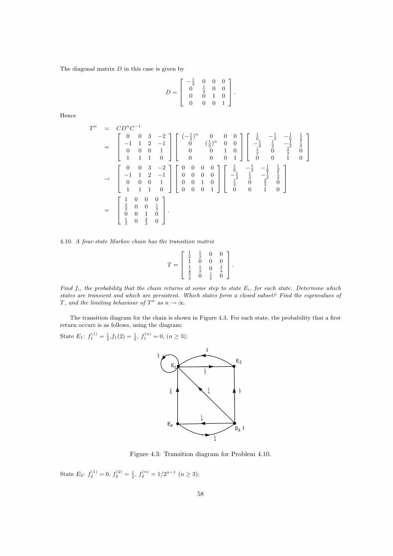
The diagonal matrix D in this case is given by
D =
− 1
20 0 0
0 12
0 00 0 1 00 0 0 1
.
Hence
T n = CDnC−1
=
0 0 3 −2−1 1 2 −10 0 0 11 1 1 0
(− 12)n 0 0 0
0 ( 12)n 0 0
0 0 1 00 0 0 1
16
− 12
− 16
12
− 12
12
− 12
12
13
0 23
00 0 1 0
→
0 0 3 −2−1 1 2 −10 0 0 11 1 1 0
0 0 0 00 0 0 00 0 1 00 0 0 1
16
− 12
− 16
12
− 12
12
− 12
12
13
0 23
00 0 1 0
=
1 0 0 023
0 0 13
0 0 1 013
0 23
0
.
4.10. A four-state Markov chain has the transition matrix
T =
12
12
0 01 0 0 014
12
0 14
34
0 14
0
.
Find fi, the probability that the chain returns at some step to state Ei, for each state. Determine whichstates are transient and which are persistent. Which states form a closed subset? Find the eigenvalues ofT , and the limiting behaviour of T n as n →∞.
The transition diagram for the chain is shown in Figure 4.3. For each state, the probability that a firstreturn occurs is as follows, using the diagram:
State E1: f(1)1 = 1
2,f1(2) = 1
2, f
(n)1 = 0, (n ≥ 3);
E1
E2
E3
12
1
1E4
34
14
14
12
14
12
Figure 4.3: Transition diagram for Problem 4.10.
State E2: f(1)2 = 0, f
(2)2 = 1
2, f
(n)2 = 1/2n−1 (n ≥ 3);
58
State E3: f(1)3 = 0, f
(2)3 = 1
42 , f(n)3 = 1/4n, (n ≥ 3):
State E4: f(n)4 = f
(n)3 for all n.
The probability of a return at any stage is
fn =
∞∑r=1
f (n)r ,
for each n. Therefore
f1 =1
2+
1
2= 1, f2 =
1
2+
1
22+
1
23+ · · · = 1,
f3 = f4 =1
42+
1
43+ · · · = 1
12,
summing geometric series for f2 and f3. Hence E1 and E2 are persistent states , but E3 and E4 aretransient.
The eigenvalues pf T are λ1 = − 12, λ2 = − 1
4, λ3 = 1
4, and λ4 = 1. The corresponding eigenvectors are
r1 =
− 1
323
−11
, r2 =
00−11
, r3 =
0011
, r4 =
1111
.
Therefore D, C and its inverse are given by
D =
− 12
0 0 0
0 − 14
0 0
0 0 14
0
0 0 0 1
, C =
− 13
0 0 123
0 0 1
−1 −1 1 1
1 1 1 1
, C−1 =
−1 1 0 0
1 −1 − 12
12
− 23
− 13
12
12
23
13
0 0
Hence
limn→∞
T n =
− 13
0 0 123
0 0 1
−1 −1 1 1
1 1 1 1
0 0 0 0
0 0 0 0
0 0 0 0
0 0 0 1
−1 1 0 0
1 −1 − 12
12
− 23
− 13
12
12
23
13
0 0
=
23
− 13
0 023
− 13
0 023
− 13
0 023
− 13
0 0
4.11. A six-state Markov chain has the transition matrix
T =
14
12
0 0 0 14
0 0 0 0 0 10 1
40 1
412
00 0 0 0 1 00 0 0 1
212
00 0 0 1
212
00 0 1 0 0 0
.
Sketch its transition diagram. From the diagram which states do you think are transient and which doyou think are persistent? Which states form a closed subset? Determine the invariant distribution in thesubset.
Intuitively E1, E2, E3 and E6 are transient since paths can always escape through E3 and not return.
59
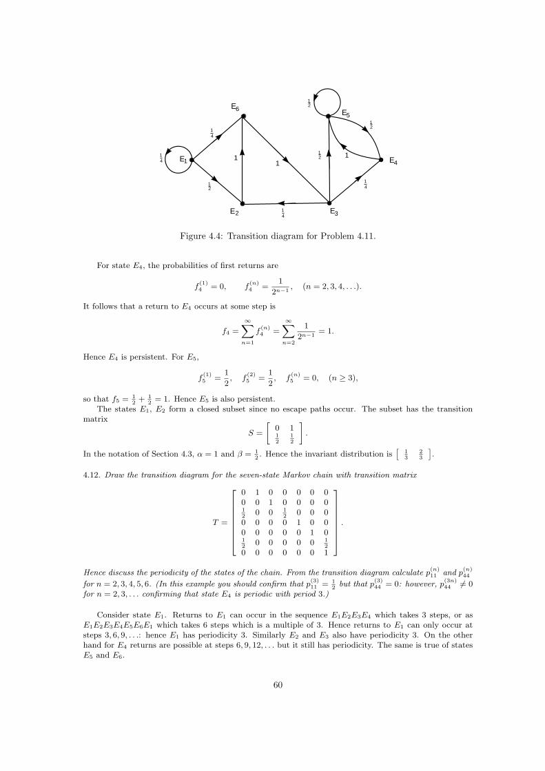
E1
E2 E3
12
11
E414
14
12
14
E5E6
1
14
12
12
Figure 4.4: Transition diagram for Problem 4.11.
For state E4, the probabilities of first returns are
f(1)4 = 0, f
(n)4 =
1
2n−1, (n = 2, 3, 4, . . .).
It follows that a return to E4 occurs at some step is
f4 =
∞∑n=1
f(n)4 =
∞∑n=2
1
2n−1= 1.
Hence E4 is persistent. For E5,
f(1)5 =
1
2, f
(2)5 =
1
2, f
(n)5 = 0, (n ≥ 3),
so that f5 = 12
+ 12
= 1. Hence E5 is also persistent.The states E1, E2 form a closed subset since no escape paths occur. The subset has the transition
matrix
S =
[0 112
12
].
In the notation of Section 4.3, α = 1 and β = 12. Hence the invariant distribution is
[13
23
].
4.12. Draw the transition diagram for the seven-state Markov chain with transition matrix
T =
0 1 0 0 0 0 00 0 1 0 0 0 012
0 0 12
0 0 00 0 0 0 1 0 00 0 0 0 0 1 012
0 0 0 0 0 12
0 0 0 0 0 0 1
.
Hence discuss the periodicity of the states of the chain. From the transition diagram calculate p(n)11 and p
(n)44
for n = 2, 3, 4, 5, 6. (In this example you should confirm that p(3)11 = 1
2but that p
(3)44 = 0: however, p
(3n)44 6= 0
for n = 2, 3, . . . confirming that state E4 is periodic with period 3.)
Consider state E1. Returns to E1 can occur in the sequence E1E2E3E4 which takes 3 steps, or asE1E2E3E4E5E6E1 which takes 6 steps which is a multiple of 3. Hence returns to E1 can only occur atsteps 3, 6, 9, . . .: hence E1 has periodicity 3. Similarly E2 and E3 also have periodicity 3. On the otherhand for E4 returns are possible at steps 6, 9, 12, . . . but it still has periodicity. The same is true of statesE5 and E6.
60
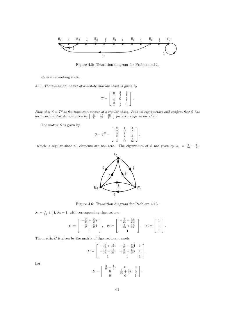
E1 E2 E3 E4 E5 E61 E71
1
1 112
12
12
12
Figure 4.5: Transition diagram for Problem 4.12.
E7 is an absorbing state.
4.13. The transition matrix of a 3-state Markov chain is given by
T =
0 34
14
12
0 12
34
14
0
.
Show that S = T 2 is the transition matrix of a regular chain. Find its eigenvectors and confirm that S hasan invariant distribution given by
[1437
1337
1037
]for even steps in the chain.
The matrix S is given by
S = T 2 =
916
116
38
38
12
18
18
916
516
,
which is regular since all elements are non-zero. The eigenvalues of S are given by λ1 = 316− 1
4i,
E1
E2 E3
14
12
34
12
34
14
Figure 4.6: Transition diagram for Problem 4.13.
λ2 = 316
+ 14i, λ3 = 1, with corresponding eigenvectors
r1 =
− 16
25+ 13
25i
− 1625− 13
25i
1
, r2 =
− 2
25− 14
25i
− 225
+ 1425
i
1
, r3 =
1
1
1
.
The matrix C is given by the matrix of eigenvectors, namely
C =
− 16
25+ 13
25i − 2
25− 14
25i 1
− 1625− 13
25i − 2
25+ 14
25i 1
1 1 1
.
Let
D =
[ 316− 1
4i 0 0
0 316
+ 14i 0
0 0 1
].
61
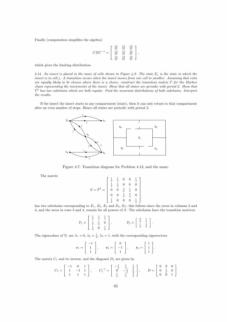
Finally (computation simplifies the algebra)
CDC−1 =
1437
1337
1037
1437
1337
1037
1437
1337
1037
,
which gives the limiting distribution.
4.14. An insect is placed in the maze of cells shown in Figure 4.9. The state Ej is the state in which theinsect is in cell j. A transition occurs when the insect moves from one cell to another. Assuming that exitsare equally likely to be chosen where there is a choice, construct the transition matrix T for the Markovchain representing the movements of the insect. Show that all states are periodic with period 2. Show thatT 2 has two subchains which are both regular. Find the invariant distributions of both subchains. Interpretthe results.
If the insect the insect starts in any compartment (state), then it can only return to that compartmentafter an even number of steps. Hence all states are periodic with period 2.
E1
E2
E3
12
1
1
E4
12
12
E5
12
12
12
12
E4 E2
E1
E3E5
Figure 4.7: Transition diagram for Problem 4.13, and the maze.
The matrix
S = T 2 =
12
14
0 0 14
12
12
0 0 0
0 0 34
14
0
0 0 14
34
012
0 0 0 12
has two subchains corresponding to E1, E2, E5 and E3, E4: this follows since the zeros in columns 3 and4, and the zeros in rows 3 and 4, remain for all powers of S. The subchains have the transition matrices
T1 =
12
14
14
12
12
012
0 12
, T2 =
[34
14
14
34
].
The eigenvalues of T1 are λ1 = 0, λ2 = 12, λ3 = 1, with the corresponding eigenvectors
r1 =
[ −111
], r2 =
[0−11
], r3 =
[111
].
The matrix C1 and its inverse, and the diagonal D1 are given by
C1 =
[ −1 0 11 −1 11 1 1
], C−1
1 =
[ − 12
14
14
0 − 12
12
12
14
14
], D =
[0 0 00 1
20
0 0 1
]
62
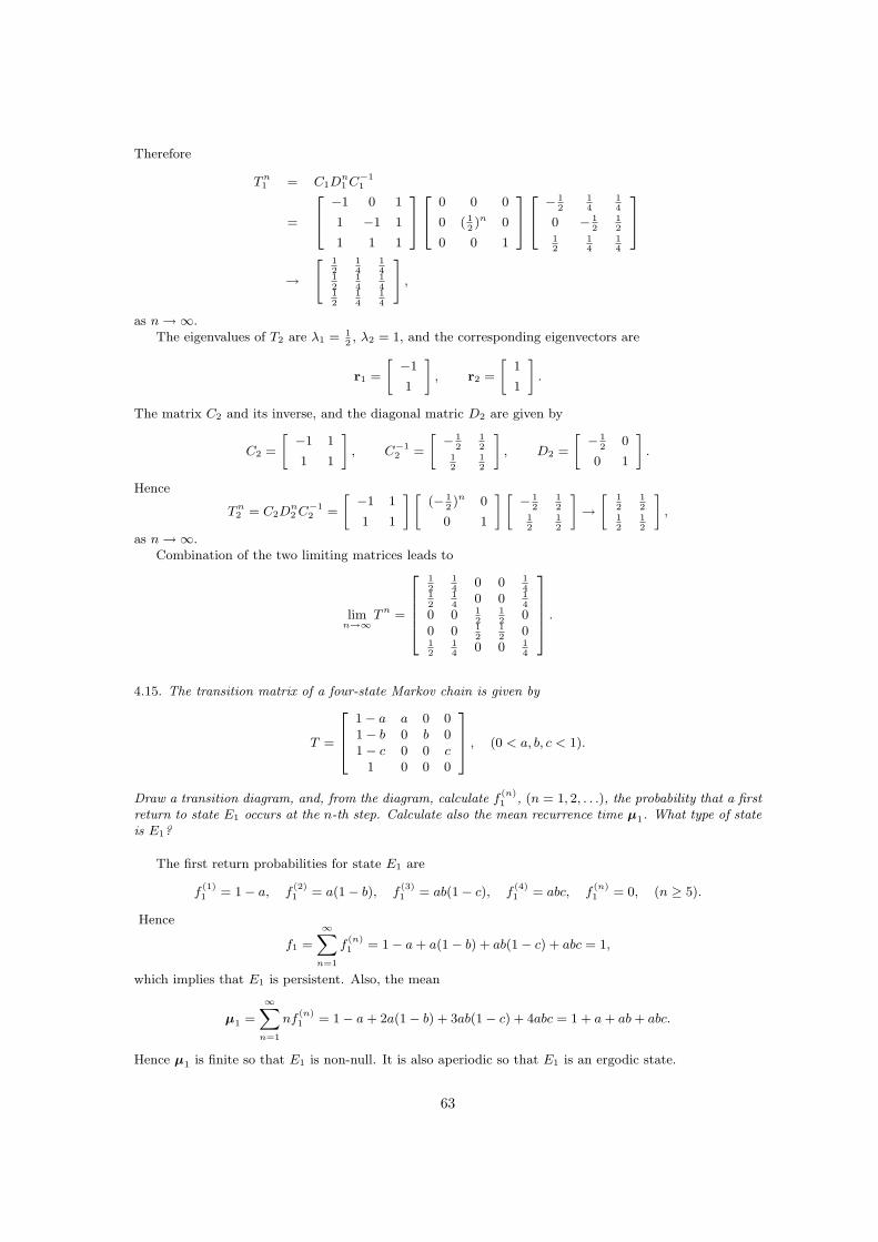
Therefore
T n1 = C1D
n1 C−1
1
=
−1 0 1
1 −1 1
1 1 1
0 0 0
0 ( 12)n 0
0 0 1
− 1
214
14
0 − 12
12
12
14
14
→[ 1
214
14
12
14
14
12
14
14
],
as n →∞.The eigenvalues of T2 are λ1 = 1
2, λ2 = 1, and the corresponding eigenvectors are
r1 =
[ −1
1
], r2 =
[1
1
].
The matrix C2 and its inverse, and the diagonal matric D2 are given by
C2 =
[ −1 1
1 1
], C−1
2 =
[ − 12
12
12
12
], D2 =
[ − 12
0
0 1
].
Hence
T n2 = C2D
n2 C−1
2 =
[ −1 1
1 1
][(− 1
2)n 0
0 1
][ − 12
12
12
12
]→
[12
12
12
12
],
as n →∞.Combination of the two limiting matrices leads to
limn→∞
T n =
12
14
0 0 14
12
14
0 0 14
0 0 12
12
00 0 1
212
012
14
0 0 14
.
4.15. The transition matrix of a four-state Markov chain is given by
T =
1− a a 0 01− b 0 b 01− c 0 0 c
1 0 0 0
, (0 < a, b, c < 1).
Draw a transition diagram, and, from the diagram, calculate f(n)1 , (n = 1, 2, . . .), the probability that a first
return to state E1 occurs at the n-th step. Calculate also the mean recurrence time µ1. What type of stateis E1?
The first return probabilities for state E1 are
f(1)1 = 1− a, f
(2)1 = a(1− b), f
(3)1 = ab(1− c), f
(4)1 = abc, f
(n)1 = 0, (n ≥ 5).
Hence
f1 =
∞∑n=1
f(n)1 = 1− a + a(1− b) + ab(1− c) + abc = 1,
which implies that E1 is persistent. Also, the mean
µ1 =
∞∑n=1
nf(n)1 = 1− a + 2a(1− b) + 3ab(1− c) + 4abc = 1 + a + ab + abc.
Hence µ1 is finite so that E1 is non-null. It is also aperiodic so that E1 is an ergodic state.
63
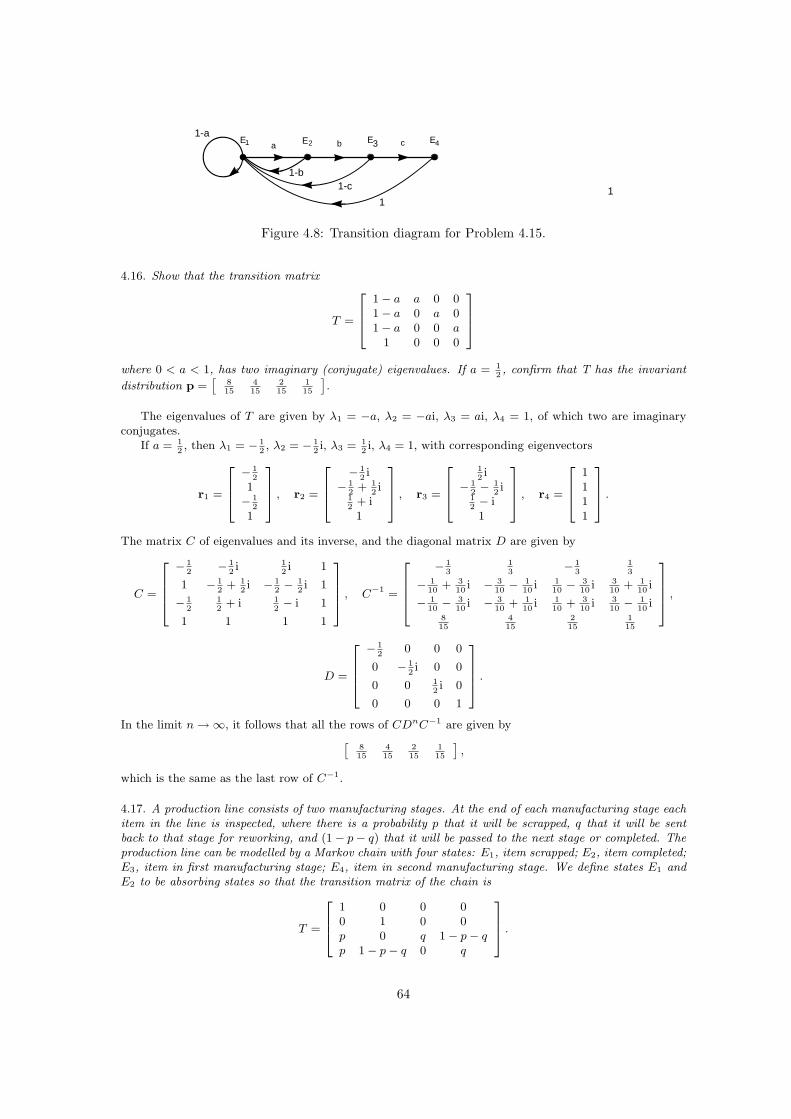
E1 E2 E3 E4
1-b
111-c
1-aa b c
Figure 4.8: Transition diagram for Problem 4.15.
4.16. Show that the transition matrix
T =
1− a a 0 01− a 0 a 01− a 0 0 a
1 0 0 0
where 0 < a < 1, has two imaginary (conjugate) eigenvalues. If a = 12, confirm that T has the invariant
distribution p =[
815
415
215
115
].
The eigenvalues of T are given by λ1 = −a, λ2 = −ai, λ3 = ai, λ4 = 1, of which two are imaginaryconjugates.
If a = 12, then λ1 = − 1
2, λ2 = − 1
2i, λ3 = 1
2i, λ4 = 1, with corresponding eigenvectors
r1 =
− 1
2
1− 1
2
1
, r2 =
− 12i
− 12
+ 12i
12
+ i1
, r3 =
12i
− 12− 1
2i
12− i1
, r4 =
1111
.
The matrix C of eigenvalues and its inverse, and the diagonal matrix D are given by
C =
− 12
− 12i 1
2i 1
1 − 12
+ 12i − 1
2− 1
2i 1
− 12
12
+ i 12− i 1
1 1 1 1
, C−1 =
− 13
13
− 13
13
− 110
+ 310
i − 310− 1
10i 1
10− 3
10i 3
10+ 1
10i
− 110− 3
10i − 3
10+ 1
10i 1
10+ 3
10i 3
10− 1
10i
815
415
215
115
,
D =
− 12
0 0 0
0 − 12i 0 0
0 0 12i 0
0 0 0 1
.
In the limit n →∞, it follows that all the rows of CDnC−1 are given by
[815
415
215
115
],
which is the same as the last row of C−1.
4.17. A production line consists of two manufacturing stages. At the end of each manufacturing stage eachitem in the line is inspected, where there is a probability p that it will be scrapped, q that it will be sentback to that stage for reworking, and (1− p− q) that it will be passed to the next stage or completed. Theproduction line can be modelled by a Markov chain with four states: E1, item scrapped; E2, item completed;E3, item in first manufacturing stage; E4, item in second manufacturing stage. We define states E1 andE2 to be absorbing states so that the transition matrix of the chain is
T =
1 0 0 00 1 0 0p 0 q 1− p− qp 1− p− q 0 q
.
64
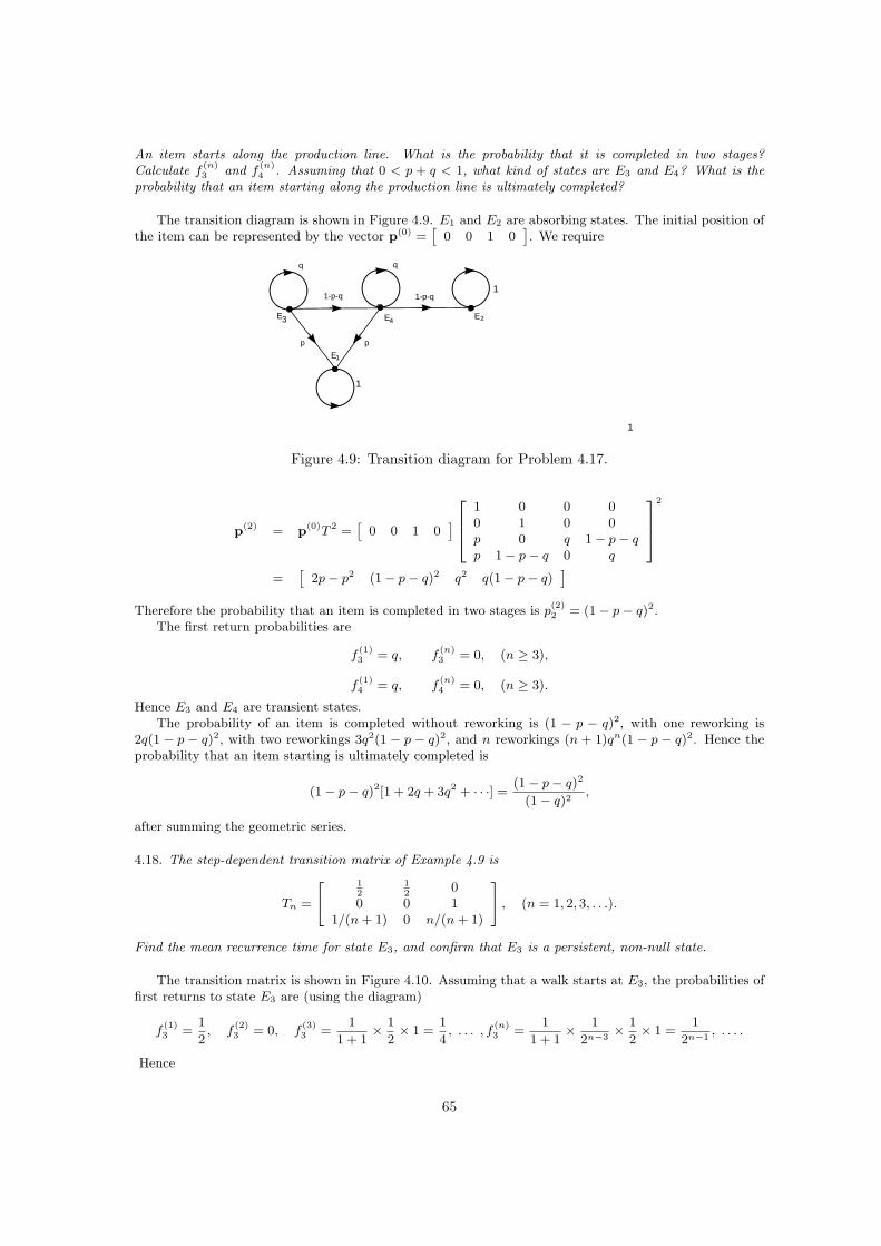
An item starts along the production line. What is the probability that it is completed in two stages?Calculate f
(n)3 and f
(n)4 . Assuming that 0 < p + q < 1, what kind of states are E3 and E4? What is the
probability that an item starting along the production line is ultimately completed?
The transition diagram is shown in Figure 4.9. E1 and E2 are absorbing states. The initial position ofthe item can be represented by the vector p(0) =
[0 0 1 0
]. We require
E1
E2E3 E4
1
1
1
q q
p p
1-p-q 1-p-q
Figure 4.9: Transition diagram for Problem 4.17.
p(2) = p(0)T 2 =[
0 0 1 0]
1 0 0 00 1 0 0p 0 q 1− p− qp 1− p− q 0 q
2
=[
2p− p2 (1− p− q)2 q2 q(1− p− q)]
Therefore the probability that an item is completed in two stages is p(2)2 = (1− p− q)2.
The first return probabilities are
f(1)3 = q, f
(n)3 = 0, (n ≥ 3),
f(1)4 = q, f
(n)4 = 0, (n ≥ 3).
Hence E3 and E4 are transient states.The probability of an item is completed without reworking is (1 − p − q)2, with one reworking is
2q(1 − p − q)2, with two reworkings 3q2(1 − p − q)2, and n reworkings (n + 1)qn(1 − p − q)2. Hence theprobability that an item starting is ultimately completed is
(1− p− q)2[1 + 2q + 3q2 + · · ·] =(1− p− q)2
(1− q)2,
after summing the geometric series.
4.18. The step-dependent transition matrix of Example 4.9 is
Tn =
[ 12
12
00 0 1
1/(n + 1) 0 n/(n + 1)
], (n = 1, 2, 3, . . .).
Find the mean recurrence time for state E3, and confirm that E3 is a persistent, non-null state.
The transition matrix is shown in Figure 4.10. Assuming that a walk starts at E3, the probabilities offirst returns to state E3 are (using the diagram)
f(1)3 =
1
2, f
(2)3 = 0, f
(3)3 =
1
1 + 1× 1
2× 1 =
1
4, . . . , f
(n)3 =
1
1 + 1× 1
2n−3× 1
2× 1 =
1
2n−1, . . . .
Hence
65
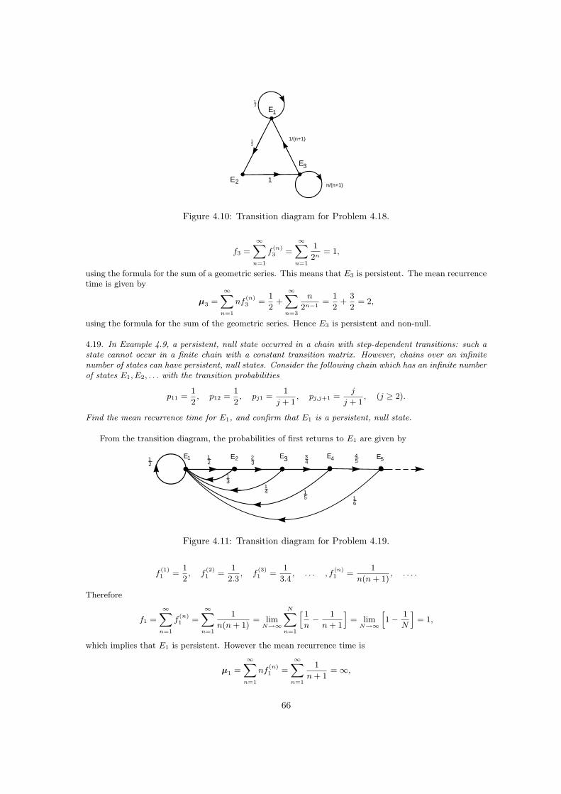
E1
E2
E3
12
12
1n/(n+1)
1/(n+1)
Figure 4.10: Transition diagram for Problem 4.18.
f3 =
∞∑n=1
f(n)3 =
∞∑n=1
1
2n= 1,
using the formula for the sum of a geometric series. This means that E3 is persistent. The mean recurrencetime is given by
µ3 =
∞∑n=1
nf(n)3 =
1
2+
∞∑n=3
n
2n−1=
1
2+
3
2= 2,
using the formula for the sum of the geometric series. Hence E3 is persistent and non-null.
4.19. In Example 4.9, a persistent, null state occurred in a chain with step-dependent transitions: such astate cannot occur in a finite chain with a constant transition matrix. However, chains over an infinitenumber of states can have persistent, null states. Consider the following chain which has an infinite numberof states E1, E2, . . . with the transition probabilities
p11 =1
2, p12 =
1
2, pj1 =
1
j + 1, pj,j+1 =
j
j + 1, (j ≥ 2).
Find the mean recurrence time for E1, and confirm that E1 is a persistent, null state.
From the transition diagram, the probabilities of first returns to E1 are given by
E1 E2 E3 E4 E512
12
13
23
34
45
14 1
5 16
Figure 4.11: Transition diagram for Problem 4.19.
f(1)1 =
1
2, f
(2)1 =
1
2.3, f
(3)1 =
1
3.4, . . . , f
(n)1 =
1
n(n + 1), . . . .
Therefore
f1 =
∞∑n=1
f(n)1 =
∞∑n=1
1
n(n + 1)= lim
N→∞
N∑n=1
[1
n− 1
n + 1
]= lim
N→∞
[1− 1
N
]= 1,
which implies that E1 is persistent. However the mean recurrence time is
µ1 =
∞∑n=1
nf(n)1 =
∞∑n=1
1
n + 1= ∞,
66
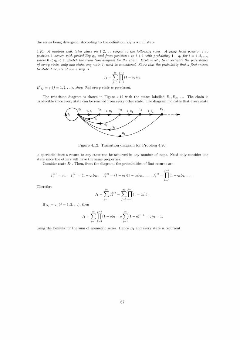
the series being divergent. According to the definition, E1 is a null state.
4.20. A random walk takes place on 1, 2, . . . subject to the following rules. A jump from position i toposition 1 occurs with probability qi, and from position i to i + 1 with probability 1 − qi for i = 1, 2, . . .,where 0 < qi < 1. Sketch the transition diagram for the chain. Explain why to investigate the persistenceof every state, only one state, say state 1, need be considered. Show that the probability that a first returnto state 1 occurs at some step is
f1 =
∞∑j=1
j−1∏k=1
(1− qk)qj .
If qj = q (j = 1, 2, . . .), show that every state is persistent.
The transition diagram is shown in Figure 4.12 with the states labelled E1, E2, . . .. The chain isirreducible since every state can be reached from every other state. The diagram indicates that every state
E1 E2 E3 E4 E5
q1
q5
q41-q31-q21-q11-
q4
q3
q2
Figure 4.12: Transition diagram for Problem 4.20.
is aperiodic since a return to any state can be achieved in any number of steps. Need only consider onestate since the others will have the same properties.
Consider state E1. Then, from the diagram, the probabilities of first returns are
f(1)1 = q1, f
(2)1 = (1− q1)q2, f
(3)1 = (1− q1)(1− q2)q3, . . . , f
(j)1 =
j−1∏k=1
(1− qk)qj , . . . .
Therefore
f1 =
∞∑j=1
f(j)1 =
∞∑j=1
j−1∏k=1
(1− qk)qj .
If qj = q, (j = 1, 2, . . .), then
f1 =
∞∑j=1
j−1∏k=1
(1− q)q = q
∞∑j=1
(1− q)j−1 = q/q = 1,
using the formula for the sum of geometric series. Hence E1 and every state is recurrent.
67
Chapter 5
Poisson processes
5.1. The number of cars which pass a roadside speed camera within a specified hour is assumed to be aPoisson process with parameter λ = 92 per hour. It is also found that 1% of cars exceed the designatedspeed limit. What are the probabilities that (a) at least one car exceeds the speed limit, (b) at least two carsexceed the speed limit in the hour.
With λ = 92 in the Poisson process, the mean number of cars in the hour is 92 × 1 = 92. Of these,on average, 0.92 cars exceed the speed limit. Assume that the cars which exceed the limit form a Poissonprocess with parameter λ1 = 0.92. Let N(t) be a random variable of the number of cars exceeding thespeed limit by time t measured from the beginning of the hour.
(a) The probability that at least one car has exceeded the limit within the hour is
1−P(N(t) < 1) = 1− e−λ1 = 1− 0.398 = 0.602.
(b) The probability that at least two cars have exceeded the limit within the hour is
1−P(N(t) < 2) = 1− e−λ1 − λ1e−λ1 = 1− 0.398− 0.367 = 0.235.
5.2. If the between-event time in a Poisson process has an exponential distribution with parameter λ withdensity λe−λt, then the probabilitythat the time for the next event to occur is at least t1 is
P{Qt > t} = e−λt.
Show that, if t1, t2 ≥ 0, then
P{Qt > t1 + t2|Qt > t1} = P{Qt > t2}.
What does this result imply about the Poisson process and its memory of past events?
By formula (1.2) on conditional probability
P(Q > t1 + t2|Q > t1) =P(Q > t1 + t2 ∩Q > t1)
P(Q > t1)=
P(Q > t1 + t2)
P(Q > t1)
=e−λ(t1+t2)
e−λt1= e−λt2
= P(Q > t2)
The result shows the loss of memory property of the Poisson process.
5.3. The number of cars which pass a roadside speed camera are assumed to behave as a Poisson processwith intensity λ. It is found that the probability that a car exceeds the designated speed limit is σ.
(a) Show that the number of cars which break the speed limit also form a Poisson process.
68
(b) If n cars pass the camera in time t, find the probability function for the number of cars which exceedthe speed limit.
(a) Let N(t) be the random variable representing m the number of speeding cars which have occurred intime t. The probability qn(t) = P(N(t) = m) satisfies
qn(t + δt) ≈ qn−1(t)λσδt + qn(t)(1− λσδt),
where λσδt is the probability that a speeding car appears in the time δt. This is the equation for a Poissonprocess with intensity λσ.(b) Of the n cars the number of ways in which m speeding cars can be arranged is
n!
m!(n−m)!=
(n
m
).
The probability that any individual event occurs is(
n
m
)σm(1− σ)n−m, (m = 0, 1, 2, . . . , n),
which is the binomial distribution.
5.4. The variance of a random variable Xt is given by
V(Xt) = E(X2t )−E(Xt)
2.
In terms of the generating function G(s, t), show that
V(Xt) =
[∂
∂s
(s∂G(s, t)
∂s
)−
(∂G(s, t)
∂s
)2]
s=1
.
(an alternative formula to (5.20)). Obtain the variance for the Poisson process using its generating function
G(s, t) = eλ(s−1)t
given by eqn (5.17), and check your answer with that given in Problem 5.3.
The assumption is that the random variable Xt is a function of the time t. Let pn(t) = P(Xt = n).The probability generating function G(s, t) becomes a function of two variables s and t. It is defined by
G(s, t) =
∞∑n=0
pn(t)sn.
The mean of Xt is given by
E(Xt) =
∞∑n=1
npn(t) =∂G(s, t)
∂s
∣∣∣∣s=1
The mean of X2t is given by
E(X2t ) =
∞∑n=1
n2pn(t) =∂
∂s
(s∂G(s, t)
∂s
)
s=1
.
Hence
V(Xt) =
[∂
∂s
(s∂G(s, t)
∂s
)−
(∂G(s, t)
∂s
)2]
s=1
.
For the Poisson process G(s, t) = eλ(s−1)t. Then
E(Xt) =∂
∂s[eλ(s−1)t]
∣∣∣s=1
= λt,
69
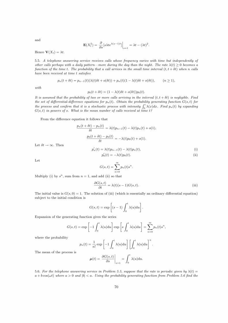
and
E(X2t ) =
∂
∂s[sλteλ(s−1)t]
∣∣∣s=1
= λt− (λt)2.
Hence V(Xt) = λt.
5.5. A telephone answering service receives calls whose frequency varies with time but independently ofother calls perhaps with a daily pattern—more during the day than the night. The rate λ(t) ≥ 0 becomes afunction of the time t. The probability that a call arrives in the small time interval (t, t + δt) when n callshave been received at time t satisfies
pn(t + δt) = pn−1(t)(λ(t)δt + o(δt)) + pn(t)(1− λ(t)δt + o(δt)), (n ≥ 1),
withp0(t + δt) = (1− λ(t)δt + o(δt))p0(t).
It is assumed that the probability of two or more calls arriving in the interval (t, t + δt) is negligible. Findthe set of differential-difference equations for pn(t). Obtain the probability generating function G(s, t) for
the process and confirm that it is a stochastic process with intensity∫ t
0λ(x)dx. Find pn(t) by expanding
G(s, t) in powers of s. What is the mean number of calls received at time t?
From the difference equation it follows that
pn(t + δt)− pn(t)
δt= λ(t)pn−1(t)− λ(t)pn(t) + o(1),
p0(t + δt)− p0(t)
δt= −λ(t)p0(t) + o(1).
Let δt →∞. Thenp′n(t) = λ(t)pn−1(t)− λ(t)pn(t), (i)
p′0(t) = −λ(t)p0(t). (ii)
Let
G(s, t) =
∞∑n=0
pn(t)sn.
Multiply (i) by sn, sum from n = 1, and add (ii) so that
∂G(s, t)
∂t= λ(t)(s− 1)G(s, t). (iii)
The initial value is G(s, 0) = 1. The solution of (iii) (which is essentially an ordinary differential equation)subject to the initial condition is
G(s, t) = exp
[(s− 1)
∫ t
0
λ(u)du
].
Expansion of the generating function gives the series
G(s, t) = exp
[−1
∫ t
0
λ(u)du
]exp
[s
∫ t
0
λ(u)du
]=
∞∑n=0
pn(t)sn,
where the probability
pn(t) =1
n!exp
[−1
∫ t
0
λ(u)du
][∫ t
0
λ(u)du
]n
.
The mean of the process is
µ(t) =∂G(s, t)
∂s
∣∣∣∣s=1
=
∫ t
0
λ(u)du.
5.6. For the telephone answering service in Problem 5.5, suppose that the rate is periodic given by λ(t) =a + b cos(ωt) where a > 0 and |b| < a. Using the probability generating function from Problem 5.6 find the
70
probability that n calls have been received at time t. Find also the mean number of calls received at time t.Sketch graphs of p0(t), p1(t) and p2(t) where a = 0.5, b = 0.2 and ω = 1.
Using the results from Problem 5.5,
G(s, t) = exp
[(s− 1)
∫ t
0
(a + b cos ωu)du
]= exp[(s− 1)(at + (b/ω) sin ωt)].
Hence
pn(t) =1
n!e−[at+(b/ω) sin ωt][at + (b/ω) sin ωt]n,
and the mean isµ(t) = at + (b/ω) sin ωt.
The first three probabilities are shown in Figure 5.1.
t
p (t)
0p (t)
p (t)
1
2
Figure 5.1: Graphs of the probabilities p0(t), p1(t) and p2(t) versus t in Problem 5.6.
5.7. A Geiger counter is pre-set so that its initial reading is n0 at time t = 0. What are the initialconditions on pn(t), the probability that the reading is n at time t, and its generating function G(s, t)?Find pn(t), and the mean reading of the counter at time t.
The probability generating function for this Poisson process is (see eqn (5.16))
G(s, t) = A(s)eλ(s−1)t.
The initial condition is G(s, 0) = xn0 . Hence A(s) = sn0 and
G(s, t) = sn0eλ(s−1)t.
The power series expansion of G(s, t) is
G(s, t) =
∞∑n=n0
snλn−n0e−λt
(n− n0)!.
Hence
pn(t) = 0, (n < n0), pn(t) =(λt)n−n0e−λt
(n− n0)!, (n ≥ n0).
The mean reading at time t is given by
µ(t) =∂G(s, t)
∂s
∣∣∣∣s=1
= n0 + λt.
71
5.8. A Poisson process with probabilities
pn(t) = P[N(t) = n] =(λt)ne−λt
n!
has a random variable N(t). If λ = 0.5, calculate the following probabilities associated in the process:(a) P[N(3) = 6];(b) P[N(2.6) = 3];(c) P[N(3.7) = 4|N(2.1) = 2];(d) P[N(7)−N(3) = 3].
(a) P(N(3) = 6) = p6(3) =(0.5× 3)6e−0.5×3
6!= 0.00353.
(b) P(N(2.6) = 3) = p3(2.6) =(0.5× 2.6)3e−0.5×2.6
3!= 0.100.
(c) P[N(3.7) = 4|N(2.1) = 2] = P[N(1.6) = 2] = p2(1.6) =(0.5× 1.6)2e−0.5×1.6
2!= 0.144.
(d) P[N(7)−N(3) = 3] = P[N(4) = 3] = 0.180.
5.9. A telephone banking service receives an average of 1000 call per hour. On average a customer transac-tion takes one minute. If the calls arrive as a Poisson process, how many operators should the bank employto avoid an expected accumulation of incoming calls?
Let time t be measured in minutes . The intensity of the Poisson process λ = 1000/60 = 50/3. Theexpected inter-arrival time is
1
λ=
3
50= 0.06 minutes.
This must be covered1
0.06= 16.7 operators.
Hence 17 operators would be required to cover expected incoming calls.
5.10. A Geiger counter automatically switches off when the nth particle has been recorded, where n is fixed.The arrival of recorded particles is assumed to be a Poisson process with parameter λt. What is the expectedvalue of the switch-off times?
The probability distribution for the switch-off times is
F (t) = 1− {probabilities that 0, 1, 2, . . . , n− 1 particles recorded by time t)}
= 1− e−λt
{1 + λt + · · ·+ (λt)n−1
(n− 1)!
}
= 1− e−λt
n−1∑r=0
(λt)r
r!
Its density is, for t > 0,
f(t) =dF (t)
dt=
d
dt
{1− e−λt
n−1∑r=0
(λt)r
r!
}
= λe−λt
n−1∑r=0
(λt)n
n!− e−λt
n−1∑r=1
λntn−1
(n− 1)!
= λe−λt (λt)n−1
(n− 1)!.
72
which is gamma. Its expected value is
µ =
∫ ∞
0
tf(t)dt =
∫ ∞
0
λe−λt λn−1
(n− 1)!tndt =
λn
(n− 1)!
∫ ∞
0
e−λttndt
=1
λ(n− 1)!
∫ ∞
0
e−sds =n!
λ(n− 1)!=
n
λ.
5.11. Particles are emitted from a radioactive source, and, N(t), the random variable of the number of
particles emitted up to time t form t = 0, is a Poisson process with intensity λ. The probability that any
particle hits a certain target is p, independently of any other particle. If Mt is the random variable of the
number of particles that hit the target up to time t, show, using the law of total probability, that M(t) forms
a Poisson process with intensity λp.
For any two times t1, t2, (t2 > t1 ≥ 0), using the law of total probability, with t2 − t1 = t,
P[M(t2)−M(t1) = k] =∞∑
n=k
P[N(t2)−N(t1) = n](
n
k
)pk(1− p)n−k
=∞∑
n=k
e−λt (λt)n
n!
(n
k
)pk(1− p)n−k
= e−λt pk
(1− p)k
∞∑
n=k
(λt)n
n!
(n
k
)(1− p)n
= e−λt (pλt)k
k!
∞∑
n=k
[(1− p)λt]n−k
(n− k)!
=(λpt)ke−λpt
k!,
which is a Poisson process of intensity λp.
73
Chapter 6
Birth and death processes
6.1. A colony of cells grows from a single cell. The probability that a cell divides in a time interval δt is
λδt + o(δt).
There are no deaths. Show that the probability generating function for this death process is
G(s, t) =se−λt
1− (1− e−λt)s.
Find the probability that the original cell has not divided at time t, and the mean and variance of populationsize at time t (see Problem 5.4, for the variance formula using the probability generating function).
This is a birth process with parameter λ and initial population size 1. Hence the probability generatingfunction is (see eqn (6.12))
G(s, t) = se−λt[1− (1− e−λt)s]−1,
which satisfies the initial condition G(s, 0) = s. It follows that the probability that the population size is1 at time t is p1(t) = e−λt.
The mean population size is
µ(t) =∂G(s, t)
∂s
∣∣∣∣s=1
= eλt.
Using the generating function, the variance of the population size is
σ2 =
[∂
∂s
(s∂G(s, t)
∂s
)− ∂G(s, t)
∂s
]
s=1
= [2e2λt − eλt]− e2λt = e2λt − eλt.
6.2. A simple birth process has a constant birth-rate λ. Show that its mean population size µ(t) satisfiesthe differential equation
dµ(t)
dt= λµ(t).
How can this result be interpreted in terms of a deterministic model for a birth process?
From Section 6.3, the mean population of the birth process with initial population n0 is given byµ(t) = n0e
λt. It can be verified that
dµ
dt− λµ = n0λeλt − n0λeλt = 0,
This differential equation is a simple deterministic model for the population in a birth process, so thatthe mean population size in the stochastic process satisfies a deterministic equation. [However, this is notalways the case in the relation between stochastic and deterministic models.]
74
6.3. The probability generating function for a simple death process with death-rate µ and initial populationsize n0 is given by
G(s, t) = (1− e−µt)n0
[1 +
se−µt
1− e−µt
]n0
(see Equation (6.17)). Using the binomial theorem find the probability pn(t) for n ≤ n0. If n0 is an evennumber, find the probability that the population size has halved by time t. A large number of experimentswere undertaken with live samples with a variety of initial population sizes drawn from a common sourceand the times of the halving of deaths were recorded for each sample. What would be the expected time forthe population to halve?
The binomial expansion of G(s, t) is given by
G(s, t) = (1− e−µt)n0
[1 +
se−µt
1− e−µt
]n0
= (1− e−µt)n0
n0∑n=0
(n0
n
)e−nµtsn
(1− e−µt)n
From this series, the coefficient of sn is
pn(t) = (1− e−µt)n0−ne−nµt
(n0
n
), (n = 0, 1, 2, . . . , n0)
which is the probability that the population size is n at time t.Let n0 = 2m0, where m0 is an integer, which ensures that n0 is even. We require
pm0 = (1− e−µt)m0e−m0µt
(2m0
m0
).
The mean population size at time t is given by
µ = G− s(1, t) = n0e−µt.
This mean is half the initial population is n0eµt = 1
2n0, which occurs, on average, at time t = µ−1 ln 2.
6.4. A birth process has a probability generating function G(s, t) given by
G(s, t) =s
eλt + s(1− e−λt).
(a) What is the initial population size?(b) Find the probability that the population size is n at time t.(c) Find the mean and variance of the population size at time t.
(a) Since G(s, 0) = s, the initial population size is n0 = 1.(b) Expand the generating function using the binomial theorem:
G(s, t) =s
eλt + s(1− e−λt)= se−λt
∞∑n=0
sn(1− e−λt)n.
The coefficients give the required probabilities:
p0(t) = 0, pn(t) = e−λt(1− e−λt)n−1.
(c) Since
∂G(s, t)
∂s
∣∣∣∣s=1
=eλt
[eλt + s(1− eλt)]2
∣∣∣∣s=1
= eλt. (i)
Hence the mean population size is µ = eλt.
75
From (i),
∂2G(s, t)
∂s2
∣∣∣∣s=1
=−2eλt(1− eλt)
[eλt + s(1− eλt)]3
∣∣∣∣s=1
= −2eλt(1− eλt).
Hence the variance is given by
V(t) =
[∂G(s, t)
∂s+ s
∂2G(s, t)
∂s2−
(∂G(s, t)
∂s
)]
s=1
= eλt − 2eλt(1− eλt)− e2λt
= e2λt − eλt.
6.5. A random process has the probability generating function
G(s, t) =(
2 + st
2 + t
)r
,
where r is a positive integer. What is the initial state of the process? Find the probability pn(t) associatedwith the generating function. What is pr(t)? Show that the mean associated with G(s, t) is
µ(t) =rt
2 + t.
Since G(s, 0) = 1, this implies that the initial size is 1.Expansion of G(s, t) using the binomial theorem leads to
G(s, t) =(
2 + st
2 + t
)r
=(
2
2 + t
)r (1 +
1
2st
)r
=(
2
2 + t
)r∞∑
n=0
(r
n
)(st
2
)n
Hence the probability that the size is n at time t is
pn(t) =(
2
2 + t
)r(
r
n
)(t
2
)n
, (n = 0, 1, 2, . . .),
With n = r,
pr(t) =(
2
2 + t
)r(
r
r
)(t
2
)r
=(
rt
2 + t
)r
.
The mean size is given by
µ(t) =∂G(s, t)
∂s
∣∣∣∣s=1
=rt(2 + st)r−1
(2 + t)r
∣∣∣∣s=1
=rt
2 + t.
6.6. In a simple birth and death process with unequal birth and death-rates λ and µ, the probability gener-ating function is given by
G(s, t) =
[µ(1− s)− (µ− λs)e−(λ−µ)t
λ(1− s)− (µ− λs)e−(λ−µ)t
]n0
,
for an initial population size n0 (see Equation (6.23)).(a) Find the mean population size at time t.(b) Find the probability of extinction at time t.(c) Show that, if λ < µ, then the probability of ultimate extinction is 1. What is it if λ > µ?(d) Find the variance of the population size.
76
(a) Let G(s, t) = [A(s, t)/B(s, t)]n0 with obvious definitions for A(s, t) and B(s, t). Then
∂G(s, t)
∂s=
[A(s, t)]n0−1
[B(s, t)]n0+1[(−µ + λe−(λ−µ)t)B(s, t)− (−λ + λe−(λ−µ)t))A(s, t)].
If s = 1, then A(1, t) = B(1, t) = −(µ− λ)e−(λ−µ)t. Therefore the mean population size is given by
µ = n0e(λ−µ)t.
(b) The probability of extinction at time t is
p0(t) = G(0, t) =
[µ− µe−(λ−µ)t
λ− µe−(λ−µ)t
]n0
.
(c) If λ < µ, then e(λ−µ)t → 0 as t →∞. Hence p0(t) → 1.If λ > µ, then p0(t) → (µ/λ)n0 as t →∞.(d) This requires a lengthy differentiation to obtain the second derivative of G(s, t): symbolic compu-
tation is very helpful. The variance is given by
V(t) = Gss(1, t) + Gs(1, t)− [Gs(1, t)]2 = n0(λ + µ)
(λ− µ)[e(λ−µ) − 1], (λ 6= µ).
6.7. In a population model, the immigration rate λn = λ, a constant, and the death rate µn = nµ. For aninitial population size n0, the probability generating function is (Example 6.3)
G(s, t) = eλs/µ exp[−λ(1− (1− s)e−µt)/µ][1− (1− s)e−µt]n0 .
Find the probability that extinction occurs at time t. What is the probability of ultimate extinction?
The probability of extinction is
p0(t) = G(0, t) = (1− e−µt)n0e−λ(1−e−µt)/µ.
The probability of ultimate extinction is
limt→∞
p0(t) = e−λ/µ.
6.8. In a general birth and death process a population is maintained by immigration at a constant rate λ,and the death rate is nµ. Using the differential-difference equations (6.26) directly, obtain the differentialequation
dµ(t)
dt+ µµ(t) = λ,
for the mean population size µ(t). Solve this equation assuming an initial population n0 and compare theanswer with that given in Example 6.3.
In terms of a generating function the mean of a process is given by
µ(t) =∑n=1
npn(t).
From (6.25) (in the book) the differential-difference equation for this immigration-death model is
dpn(t)
dt= λpn−1(t)− (λ + nµ)pn(t) + µ(n + 1)pn+1(t), (n = 1, 2, . . .).
77
Multiply this equation by n and sum over over n:
∞∑n=1
ndpn(t)
dt= λ
∞∑n=1
npn−1(t)− λ
∞∑n=1
npn(t)− µ
∞∑n=1
npn(t) + µ
∞∑n=1
n(n + 1)pn+1(t)
= λ
∞∑n=0
(n + 1)pn(t)− λµ(t)− µ
∞∑n=1
n2pn(t) + µ
∞∑n=2
n(n− 1)pn(t)
= λµ(t) + λ− λµ(t)− µµ(t)
= λ− µµ(t).
Hencedµ(t)
dt+ µµ(t) = λ.
This is a first-order linear equation with general solution
µ(t) = Ae−µt +λ
µ.
The initial condition implies A = n0 − (λ/µ). Hence
µ(t) =
(n0 − λ
µ
)e−µt +
λ
µ.
6.9. In a death process the probability of a death when the population size is n 6= 0 is a constant µ butobviously zero if the population size is zero. Verify that, if the initial population is n0, then pn(t), theprobability that the population size is n at time t is given by
p0(t) =µn0
(n0 − 1)!
∫ t
0
sn0−1e−µsds, pn(t) =(µt)n0−n
(n0 − n)!e−µt, (1 ≤ n ≤ n0),
Show that the mean time to extinction is n0/µ.
The probability that a death occurs in time δt is a constant µ independently of the population size.Hence
pn0(t + δt) = (1− µ)pn0(t), (i)
pn(t + δt) = µpn+1(t) + (1− µ)pn(t), (n = 1, . . . , n0 − 1), (ii)
p0(t + δt) = µp1(t) + p0(t). (iii)
subject to the initial conditions pn0(0) = 1, pn(0) = 0, (n = 0, 1, 2, . . . n0 − 1). Divide through each of theeqns (i) and (ii) by δt, and let t →∞ to obtain the differential-difference equations
p′n0(t) = −µpn0(t), (iv)
p′n(t) = −µpn(t) + µpn+1(t), (n = 1, 2, . . . , n0 − 1). (v)
p′0(t) = µp1(t). (vi)
From (iii) and the initial conditions,pn0(t) = Ae−µt = e−µt.
From (iv) with n = n0 − 1,
p′n0−1(t) = −µpn0−1(t) + µpn0(t) = −µpn0−1(t) + e−µt.
Subject to the initial condition pn0−1(0) = 1, this first-order linear equation has the solution
pn0(t) = µte−µt.
Repeat this process which leads to the conjecture that
pn(t) =(µt)n0−n
(n0 − n)!e−µt, (n = 1, 2, . . . , n0 − 1),
78
which can be proved by induction. The final probability satisfies
p′0(t) = µp1(t) =µn0tn0−1
(n0 − 1)!e−µt.
Direct integration gives
p0(t) =µn0
(n0 − 1)!
∫ t
0
sn0−1e−µsds. (vii)
It can be checked that p0(t) → 1 as t →∞ which confirms that extinction is certain.The probability distribution of the random variable T of the time to extinction is p0(t) = P[T ≤ t]
given by (viii). Its density is
f(t) =dp0(t)
dt=
µn0 tn0−1
(n0 − 1)!e−µt.
Hence the expected value of T is
E(T ) =
∫ ∞
0
tf(t)dt =
∫ ∞
0
µn0 tn0
(n0 − 1)!e−µt =
n0
µ,
using an integral formula for the factorial (see the Appendix in the book).
6.10. In a birth and death process the birth and death rates are given by
λn = nλ + α, µn = nµ,
where α represents a constant immigration rate. Show that the probability generating function G(s, t) ofthe process satisfies
∂G(s, t)
∂t= (λs− µ)(s− 1)
∂G(s, t)
∂s+ α(s− 1)G(s, t).
Show also that, ifG(s, t) = (µ− λs)−α/λS(s, t),
then S(s, t) satisfies∂S(s, t)
∂t= (λs− µ)(s− 1)
∂S(s, t)
∂s.
Let the initial population size be n0. Solve the partial differential equation for S(s, t) using the method ofSection 6.5 and confirm that
G(s, t) =(µ− λ)α/λ[(µ− λs)− µ(1− s)e(λ−µ)t]n0
[(µ− λs)− λ(1− s)e(λ−µ)t]n0+(α/λ).
(Remember the modified initial condition for S(s, t).)Find p0(t), the probability that the population is zero at time t (since immigration takes place even
when the population is zero there is no question of extinction in this process). Hence show that
limt→∞
p0(t) =
(µ− λ
µ
)α/λ
if λ < µ. What is the limit if λ > µ?The long term behaviour of the process for λ < µ can be investigated by looking at the limit of the
probability generating function as t →∞. Show that
limt→∞
G(s, t) =
(µ− λ
µ− λs
)α/λ
.
This is the probability generating function of a stationary distribution and it indicates that a balance hasbeen achieved the birth and immigration rates, and the death rate. What is the long term mean population?
If you want a further lengthy exercise investigate the probability generating function in the special caseλ = µ.
79
The differential-difference equations are
p′0(t) = −αp0(t) + µp1(t), (i)
p′n(t) = [(n− 1)λ + α]pn−1(t)− (nλ + α + nµ)pn(t) + (n + 1)µpn+1(t), (n = 1, 2, . . .) (ii)
Multiply (ii) by sn, sum over n ≥ 1 and add (i) leads to
∞∑n=0
p′n(t)sn =
∞∑n=1
[(n− 1)λ + α]pn−1(t)− (nλ + α + nµ)pn(t)sn
+
∞∑n=0
(n + 1)µpn+1(t)sn
Let the probability generating function be G(s, t) =∑∞
n=0pn(t)sn. Then the summations above lead to
∂G(s, t)
∂t= (λs− µ)(s− 1)
∂G(s, t)
∂s+ α(α− 1)G(s, t).
Let G(s, t) = (µ− λs)−α/λS(s, t). Then
∂G(s, t)
∂s= (µ− λs)−α/λ ∂S(s, t)
∂s+ α(µ− λs)−(α/λ)−1S(s, t),
and∂G(s, t)
∂t= (µ− λs)−α/λ ∂S(s, t)
∂t.
This transformation removes the non-derivative term to leave
∂S(s, t)
∂t= (λs− µ)(s− 1)
∂S(s, t)
∂s.
Now apply the change of variable defined by
ds
dz= (λs− µ)(s− 1)
as in Section 6.5(a). Integration gives (see eqn (6.21))
s =λ− µe(λ−µ)z
λ− λe(λ−µ)z= h(z) (say). (iii)
The initial condition is equivalent to G(s, 0) = sn0 or S(s, 0) = (µ− λs)α/λsn0 . It follows that
S(f(z), 0) =
[λ(µ− λ)
λ− λe(λ−µ)z
]α/λ [λ− µe(λ−µ)z
λ− λe(λ−µ)z
]n0
= w(z) (say).
Since S(f(z), t) = w(z + t) for any smooth function of z + t, it follows that
G(s, t) = (µ− λs)−α/λS(f(z), t) = (µ− λs)−α/λw(z + t)
= (µ− λs)−α/λ
[λ(µ− λ)
λ− λe(λ−µ)(z+t)
]α/λ [λ− µe(λ−µ)(z+t)
λ− λe(λ−µ)(z+t)
]n0
,
where z is defined by s = h(z) given by (iii). Finally
G(s, t) =(µ− λ)α/λ[(µ− λs)− µ(1− s)e(λ−µ)t]n0
[(µ− λs)− λ(1− s)e(λ−µ)t]n0+(α/λ), (iv)
as displayed in the problem.The probability that the population is zero at time t is
p0(t) = G(0, t) =(µ− λ)α/λ(µ− µe(λ−µ)t)n0
(µ− λe(λ−µ)t)n0+(α/λ).
80
If λ < µ, then
p0(t) →(
µ− λ
µ
)α/λ
.
If λ > µ, then
p0(t) =(µ− λ)α/λ(µe−(λ−µ)t − µ)n0
(µe−(λ−µ)t − λ)n0+(α/λ)→
(λ− µ
λ
)α/λ (µ
λ
)n0
,
as t →∞.The long term behaviour for λ < µ is determined by letting t →∞ in (iv) resulting in
limt→∞
G(s, t) =
(µ− λ
µ− λs
)α/λ
.
Express G(s, t) in the form
G(s, t) = (µ− λ)α/λ A(s, t)
B(s, t),
where
A(s, t) = [(µ− λs)− µ(1− s)e(λ−µ)t]n0 , B(s, t) = [(µ− λs)− λ(1− s)e(λ−µ)t]n0+(α/λ).
Then
Gs(s, t) = (µ− λ)α/λ As(s, t)B(s, t)−A(s, t)Bs(s, t)
[B(s, t)]2
For the mean we require s = 1, for which value
A(1, t) = (µ− λ)n0 , B(1, t) = (µ− λ)n0+(α/λ),
As(1, t) = n0(−λ + µe(λ−µ)t)(µ− λ)n0−1,
Bs(1, t) = (n0 + (α/λ))(−λ + λe(λ−µ)t)(µ− λ)n0+(α/λ)−1.
Hence
µ(t) = Gs(1, t) = (µ− λ)α/λ As(1, t)B(1, t)−A(1, t)Bs(1, t)
[B(1, t)]2
=n0
µ− λ[α + {n0(µ− λ)− α}e(λ−µ)t].
If λ < µ, then
µ(t) → n0α
µ− λ,
as t →∞. If λ > µ, then the mean becomes unbounded as would be expected.
6.11. In a birth and death process with immigration, the birth and death rates are respectively
λn = nλ + α, µn = nµ.
Show directly from the differential-difference equations for pn(t), that the mean population size µ(t) satisfiesthe differential equation
dµ(t)
dt= (λ− µ)µ(t) + α.
Deduce the resultµ(t) → α
µ− λ
as t →∞ if λ < µ. Discuss the design of a deterministic immigration model based on this equation.
The difference equations for the probability pn(t) are given by
p′0(t) = −αp0(t) + µp1(t), (i)
p′n(t) = [(n− 1)λ + α]pn−1(t)− [(nλ + α + nµ)pn(t) + (n + 1)µpn+1(t). (ii)
81
The mean µ(t) is given by µ(t) =∑∞
n=1npn(t). Multiply (ii) by n and sum from n = 1. Then, re-ordering
the sums
dµ(t)
dt=
∞∑n=1
np′n(t) = λ
∞∑n=2
n(n− 1)pn−1(t) + α
∞∑n=1
pn−1(t)− α
∞∑n=1
npn(t)
−(λ + µ)
∞∑n=1
n2pn(t) + µ
∞∑n=1
n(n + 1)pn+1(t)
= λ
∞∑n=1
n(n + 1)pn(t) + α
∞∑n=0
pn(t)− α
∞∑n=1
npn(t)
−(λ + µ)
∞∑n=1
n2pn(t) + µ
∞∑n=2
n(n− 1)pn(t)
= α + (λ− µ)µ(t).
The mean of the stochastic process satisfies a simple deterministic model for a birth and death processwith immigration.
6.12. In a simple birth and death process with equal birth and death rates λ, the initial population size hasa Poisson distribution with probabilities
pn(0) = e−α αn
n!(n = 0, 1, 2, . . .),
with intensity α. It could be thought of as a process in which the initial distribution has arisen as the resultof some previous process. Find the probability generating function for this process, and confirm that theprobability of extinction at time t is exp[−α/(1 + λt)] and that the mean population size is α for all t.
In Section 6.5(b), the probability generating function G(s, t) for the case in which the birth and deathrates are equal satisfies
∂G(s, t)
∂t= λ(1− s)2
∂G(s, t)
∂s.
To solve the partial differential equation, the transformation
z =1
λ(1− s), or s =
λz − 1
λz(i)
is used. The result is that G(s, t) = w(z + t) for any smooth function w. The initial condition at t = 0 is
w(z) =
∞∑n=0
pn(0)sn =
∞∑n=0
αne−α
n!sn = eα(s−1) = exp
[α
(λz − 1
λz− 1
)]= e−α/(λz),
usng the transformation (i). Hence
G(s, t) = w(z + t) = e−α/[λ(z+t)] = exp
[−α
/(1
1− s+ λt
)]= exp
[−α(1− s)
1 + λt(1− s)
]
The probability of extinction at time t is
p0(t) = G(0, t) = exp[−α/(1 + λt)].
6.13. A birth and death process takes place as follows. A single bacterium is allowed to grow and assumedto behave as a simple birth process with birth rate λ for a time t1 without any deaths. No further growththen takes place. The colony of bacteria is then allowed to die with the assumption that it is a simple deathprocess with death rate µ for a time t2. Show that the probability of extinction after the total time t1 + t2 is
∞∑n=1
eλt1(1− e−λt1)n−1(1− e−µt2)n.
82
Using the formula for the sum of a geometric series, show that this probability can be simplified to
eµt2 − 1
eλt1 + eµt2 − 1.
Suppose that at time t = t1 the population size is n. From Section 6.3, the probability that thepopulation is of size n at time t1 entirely through births is
pn(t1) = e−λt1(1− e−λt1)n−1.
From Section 6.4 on the death process, the probability that the population becomes extinct after a furthertime t2 is
q0(t2) = (1− e−µt2)n.
The probability that the population increases to n and then declines to zero is
pn(t)q0(t) = e−λt1(1− e−λt1)n−1(1− e−µt2)n
Now n can take any value equal to or greater than 1. Hence the probability of extinction through everypossible n is
s(t1, t2) =
∞∑n=1
e−λt1(1− e−λt1)n−1(1− e−µt2)n.
The probability s(t1, t2) can be expressed as a geometric series in the form
s(t1, t2) =e−λt1
1− e−λt1
∞∑n=1
[(1− e−λt1)(1− e−µt2)]n
=e−λt1
(1− e−λt1)· (1− e−λt1)(1− e−µt2)
[1− (1− e−λt1)(1− e−µt2)]
=eµt2 − 1
eλt1 + eµt2 − 1
6.14. As in the previous problem a single bacterium grows as a simple birth process with rate λ and nodeaths for a time τ . The colony numbers then decline as a simple death process with rate µ. Show that theprobability generating function for the death process is
(1− e−µt(1− s))e−λτ
1− (1− e−λτ )(1− e−µt(1− s)),
where t is measured from the time τ . Show that the mean population size during the death process is eλτ−µt.
During the birth process the generating function is (see eqn (6.12))
G(s, t) =se−λt
1− (1− e−λt)s,
assuming an initial population of 1. For the death process suppose that time restarts from t = 0, and thatthe new probability generating function is H(s, t). At t = 0,
H(s, 0) = G(s, τ) =se−λτ
1− (1− e−λτ )s.
For the death process the transformation is s = 1− e−µz, so that
H(s, 0) = w(z) =(1− e−µz)e−λτ
1− (1− e−λτ )(1− e−µz).
83
Then, in terms of s,
H(s, t) = w(z + t) =[1− e−µt(1− s)]e−λt
1− (1− e−λτ )[1− e−µt(1− s)].
The mean population size in the death process is
Hs(1, t) =[1− (1− e−λτ )]e−µt−λτ + e−λτ−µt(1− e−λτ )
[1− (1− e−λτ ]2= eλτ−µt.
6.15. For a simple birth and death process the probability generating function ( equation (6.23)) is given by
G(s, t) =
[µ(1− s)− (µ− λs)e−(λ−µ)t
λ(1− s)− (µ− λs)e−(λ−µ)t
]n0
for an initial population of n0. What is the probability that the population is (a) zero, (b) 1 at time t?
G(s, t) =
[µ(1− s)− (µ− λs)e−(λ−µ)t
λ(1− s)− (µ− λs)e−(λ−µ)t
]n0
=[{µ− µe−(λ−µ)t} − s{µ− λe−(λ−µ)t}]n0
[{λ− µe−(λ−µ)t} − s{λ− λe−(λ−µ)t}]n0
=
(µ− µe−(λ−µ)t
λ− µe−(λ−µ)t
)n0[1 + n0s
{λ− λe−(λ−µ)t
λ− µe−(λ−µ)t− µ− λe−(λ−µ)t
µ− µe−(λ−µ)t
}+ · · ·
]
The probabilities p0(t) and p1(t) are given by the first two coefficiemts in this series.
6.16. (An alternative method of solution for the probability generating function) The general solution ofthe first-order partial differential equation
A(x, y, z)∂z
∂x+ B(x, y, z)
∂z
∂y= C(x, y, z)
is f(u, v) = 0, where f is an arbitrary function, and u(x, y, z) = c1 and v(x, y, z) = c2 are two independentsolutions of
dx
A(x, y, z)=
dy
B(x, y, z)=
dz
C(x, y, z).
This is known as Cauchy’s method.Apply the method to the partial differential equation for the probability generating function for the
simple birth and death process, namely (equation (6.19))
∂G(s, t)
∂t= (λs− µ)(s− 1)
∂G(s, t)
∂s,
by solvingds
(λs− µ)(1− s)=
dt
−1=
dG
0.
Show that
u(s, t, G) = G = c1, and v(s, t, G) = e−(λ−µ)t
(1− sµλ− s
)= c2.
are two independent solutions. The general solution can be written in the form
G(s, t) = H
[e−(λ−µ)t
(1− sµλ− s
)].
Here H is a function determined by the initial condition G(s, 0) = sn0 . Find H and recover formula (6.22)for the probability generating function.
84
Note that in the birth and death equation the function C is zero. Comparing the two partial differentialequations, we have to solve
ds
(λs− µ)(1− s)=
dt
−1=
dG
0.
The second equality is simply dG = 0. This equation has a general solution which can be expressed as
u(s, t, G) ≡ G = c1.
The first equality requires the solution of the differential equation
ds
dt= −(λs− µ)(1− s).
The integration is given essentially in eqn (6.20) in the text which in terms of v can be expressed as
v(s, t, G) ≡ e−(λ−µ)t
(1− s
(µ/λ)− s
)= c2.
Hence the genetal solution is
f(u, v) = 0, or f
[G, e−(λ−µ)t
(1− s
(µ/λ)− s
)]= 0.
Alternatively, this can be written in the form
G(s, t) = H
[e−(λ−µ)t
(1− s
(µ/λ)− s
)],
where he function H is determined by initial conditions.Assuming that the initial population size is n0, then G(s, 0) = sn0 , which means that H is determined
by
H
(1− s
(µ/λ)− s
)= sn0 .
Let u = (1− s)/((µ/λ)− s). Then
H(u) =[λ− µu
λ− λu
]n0
,
which determines the functional form of H. The result follows by replacing u by
e−(λ−µ)t
(1− s
(µ/λ)− s
),
as the argument of H.
6.17. Apply the Cauchy’s method outlined in Problem 6.16 to the immigration model in Example 6.3. Inthis application the probability generating function satisfies
∂G(s, t)
∂t= λ(s− 1)G(s, t) + µ(1− s)
∂G(s, t)
∂s.
Solve the equation assuming an initial population of n0.
Reading the coefficients of the partial differential equation in Problem 6.16,
ds
µ(1− s)=
dt
−1=
dG
λ(s− 1).
Integration of the second equality gives
u(s, t, G) ≡ G +λ
µs = c1,
85
whilst the first givesv(s, t, G) = eµt(1− s) = c2.
The general solution can be expressed in the functional form
G(s, t) = −λ
µs + H(eµt(1− s)).
From the initial condition G(s, 0) = sn0 . Therefore
−λ
µs + H(1− s) = sn0 ,
so that
H(1− s) =λ
µs + sn0 .
Let u = 1− s: then
H(u) =λ
µ(1− u) + (1− u)n0 .
The result follows by replacing u by eµt(1− s) in this formula.
6.18. In a population sustained by immigration at rate λ with a simple death process with rate µ (seeExample 6.3), the probability pn(t) satisfies (equation (6. 25))
dp0(t)
dt= −λp0(t) + µp1(t),
dpn(t)
dt= λpn−1(t)− (λ + nµ)pn(t) + (n + 1)µpn+1(t).
Investigate the steady-state behaviour of the system by assuming that
pn(t) → pn, dpn(t)/dt → 0
for all n, as t → ∞. Show that the resulting difference equations for what is known as the correspondingstationary process
−λp0 + µp1 = 0,
λpn−1 − (λ + nµ)pn + (n + 1)µpn+1 = 0, (n = 1, 2, . . .)
can be solved iteratively to give
p1 =λ
µp0, p2 =
λ2
2!µ2p0, · · · pn =
λn
n!µnp0, · · · .
Using the condition∑∞
n=0pn = 1, and assuming that λ < µ, determine p0. Find the mean steady-state
population size, and compare the result with that obtained in Example 6.3.
From the steady-state difference equations
p1 =λ
µp0,
p2 =1
2µ[−λp0 + (λ + 2µ)p1] =
λ2
2!µ2,
p3 =1
3µ[−λp1 + (λ + 2µ)p2] =
λ3
3!µ3p0,
and so on: the result can be confirmed by an induction proof. The requirement∑∞
n=0pn = 1 implies
∞∑n=0
(λ
µ
)n
p0 =µ
µ− λp0 = 1
if p0 = (µ− λ)/µ.
86
The mean steady state population is given by
µ =
∞∑n=1
npn =
∞∑n=1
=
∞∑n=1
np0
n!
(λ
µ
)n
=
∞∑n=1
p0
(n− 1)!
(λ
µ
)n
= p0
(λ
µ
)eλ/µ =
(µ− λ)λ
µ2eλ/µ.
6.19. In a simple birth process the probability that the population is of size n at time t given that it was n0
at time t = 0 is given by
pn(t) =
(n− 1
n0 − 1
)e−λn0t(1− e−λt)n−n0 , (n ≥ n0).
(see Section 6.3 and Figure 6.1). Show that the probability achieves its maximum value for given n and n0
when t = (1/λ) ln(n/n0). Find also the maximum value of pn(t) at this time.
Differentiating pn(t), we obtain
dpn(t)
dt= λ
(n− 1
n0 − 1
)e−λn0t(1− e−λt)n−n0−1[−n0(1− e−λt) + λ(n− n0)e
−λt].
The derivative is zero if
e−λt =n0
n, or t =
1
λln
(n
n0
).
Substituting this time back into pn(t), it follows
maxt
[pn] =
(n− 1
n0 − 1
)nn0
0
nn(n− n0)
n−n0 .
6.20. In a birth and death process with equal birth and death parameters, λ, the probability generatingfunction is (see eqn(6.24))
G(s, t) =
[1 + (λt− 1)(1− s)
1 + λt(1− s)
]n0
.
Find the mean population size at time t. Show also that its variance is 2n0λt.
The derivative of G(s, t) with respect to s is given by
Gs(s, t) =n0[λt− (λt− 1)s]n0−1
[(1 + λt)− λts]n0+1.
The mean population size at time t is
µ(t) = Gs(1, t) = n0.
We require the second derivative given by
Gss(s, t) =n0[λt− (λt− 1)s]n0−2
[(1 + λt)− λts]n0+2[n0 − 1 + 2λts + 2λ2t2(1− s)]
The variance of the population size is
V(t) = Gss(1, t) + Gs(1, t)− [Gs(1, t)]2 = [2λn0t + n20 − n0] + n0 − n2
0 = 2n0λt.
6.21. In a death process the probability that a death occurs in time δt is a time-dependent parameter µ(t)nwhen the population size is n. The pgf G(s, t) satisfies
∂G
∂t= µ(t)(1− s)
∂G
∂s.
87
as in Section 6.4. Show thatG(s, t) = [1− e−τ (1− s)]n0 ,
where
τ =
∫ t
0
µ(s)ds.
Find the mean population size at time t.In a death process it is found that the expected value of the population size at time t is given by
µ(t) =n0
1 + αt, (t ≥ 0),
where α is a positive constant. Estimate the corresponding death-rate µ(t).
Let
z =
∫ds
1− s, so that s = 1− e−z,
and
τ =
∫ t
0
µ(u)du.
The equation for the probability generating function becomes
∂G
∂τ=
∂G
∂z.
The general solution can be expressed as G(s, t) = w(z + τ) for any arbitrary differentiable function w.Initially τ = 0. Hence
G(s, 0) = sn0 = w(z) = (1− e−z)n0 ,
so thatG(s, t) = w(z + τ) = [1− e−(z+τ)]n0 = [1− e−τ (1− s)]n0 .
The mean population size at time t is given by
µ(t) = Gs(1, t) = n0e−τ [1− e−tau(1− s)]n0−1
∣∣s=1
= n0e−τ = n0 exp
[−
∫ t
0
µ(u)du
].
Given the mean
µ(t) =n0
1 + αt= n0 exp
[−
∫ t
0
µ(u)du
], (i)
it follows that the death-rate is µ(t) = α/(1 + αt), which can be obtained by differentiating both sides (i)with rspect to t
6.22. A population process has a probability generating function G(s, t) which satisfies the equation
e−t ∂G
∂t= λ(s− 1)2
∂G
∂s.
If, at time t = 0, the population size is n0, show that
G(s, t) =
[1 + (1− s)(λet − λ− 1)
1 + λ(1− s)(et − 1)
]n0
.
Find the mean population size at time t, and the probability of ultimate extinction.
The generating function satisfies
e−t ∂G
∂t= λ(x− 1)2
∂G
∂s.
Let
τ =
∫ t
0
eudu, z =
∫ds
λ(s− 1)2.
88
The transformations are τ = et − 1 and s = (λz − 1)/(λz). The transformed partial differential equationhas the general solution G(s, t) = w(z + τ). The initial condition is
G(s, 0) = sn0 =(1− 1
λz
)n0
= w(z).
Hence
G(s, t) =
(1− 1
λ(z + τ)
)n0
=
[1− s− 1
−1 + λ(s− 1)(et − 1)
]n0
=
[(s− 1)(λet − λ− 1)− 1
λ(s− 1)(et − 1)− 1
]n0
as required.The mean population size is
µ(t) = Gs(1, t) = n0.
The probability of extinction at time t is
p0(t) = G(0, t) =
[λ(et − 1)
λ(et − 1) + 1
]n0
→ 1
as t →∞.
6.23. A population process has a probability generating function given by
G(s, t) =1− µe−t(1− s)
1 + µe−t(1− s),
where µ is a parameter. Find the mean of the population size at time t, and its limit as t → ∞. ExpandG(s, t) in powers of s, determine the probability that the population size is n at time t.
We require the derivative
Gs(s, t) =µe−t[1 + µe−t(1− s)] + µe−t(1− s)[1− µe−t(1− s)]
[1 + µe−t(1− s)]2
=2µe−t
[1 + µe−t(1− s)]2
Then the mean population size isµ(t) = Gs(1, t) = 2µe−t.
To find the individual probabilities we require the power series expansion of G(s, t). Using a binomialexpansion
G(s, t) =
(1− µe−t
1 + µe−t
)(1 +
µe−ts
1− µe−t
)(1− µe−ts
1 + µe−t
)−1
=
(1− µe−t
1 + µe−t
)(1 +
µe−ts
1− µe−t
) ∞∑n=0
(µe−t
1 + µe−t
)n
sn
=
(1− µe−t
1 + µe−t
)[ ∞∑n=0
(µe−t
1 + µe−t
)n
sn +
(µe−t
1− µe−t
) ∞∑n=1
(µe−t
1 + µe−t
)n
sn+1
]
the coefficients of the powers sn give the following probabilities:
p0(t) =1− µe−t
1 + µe−t,
pn(t) =1− µe−t
1 + µe−t
[µne−nt
(1 + µe−t)n+
µne−nt
(1 + µe−t)n−1
1
(1− µe−t)
]=
2µne−nt
(1 + µe−t)n+1, (n ≥ 1).
89
6.24. In a birth and death process with equal rates λ, the probability generating function is given by (seeeqn (6.24))
G(s, t) =
[λ(z + t)− 1
λ(z + t)
]n0
=
[1 + (λt− 1)(1− s)
1 + λt(1− s)
]n0
,
where n0 is the initial population size. Show that pi, the probability that the population size is i at time t,is given by
pi(t) =
i∑m=0
(n0
m
)(n0 + i−m− 1
i−m
)α(t)mβ(t)n0+i−m
if i ≤ n0, and by
pi(t) =
n0∑m=0
(n0
m
)(n0 + i−m− 1
i−m
)α(t)mβ(t)n0+i−m
if i > n0, where
α(t) =1− λt
λt, β(t) =
λt
1 + λt.
Expand G(s, t) as a power series in terms of s using the binomial expansion:
G(s, t) =(
λt
1 + λt
)n0 [1 +
1− λt
λts]n0 [
1− λt
1 + λts]−n0
=(
λt
1 + λt
)n0n0∑
k=0
(n0
k
)αksk
∞∑j=0
(n0 + j − 1
j
)βjsj ,
where
α =1− λt
λt, β =
λt
1 + λt.
Two cases have to be considered.(a) i ≤ n0.
pi(t) =(
λt
1 + λt
)n0[(
n0
0
)α0
(n0 + i− 1
i
)βi +
(n0
1
)α
(n0 + i− 2
i− 1
)βi−1 + · · ·
+
(n0
i
)αi
(n0 − 1
0
)β0
]
=(
λt
1 + λt
)n0+i i∑m=0
(n0
m
)(n0 + i− 1−m
i−m
)(α
β
)m
=(
λt
1 + λt
)n0+i i∑m=0
(n0
m
)(n0 + i− 1−m
i−m
)(1− (λt)2
(λt)2
)m
(b) i > n0.
pi(t) =(
λt
1 + λt
)n0[(
n0
0
)α0
(n0 + i− 1
i
)βi + · · ·+
(n0
n0
)αn0
(i− 1
i− n0
)βi−n0
]
=(
λt
1 + λt
)n0+i n0∑m=0
(n0
m
)(n0 + i− 1−m
i−m
)(1− (λt)2
(λt)2
)m
6.25. We can view the birth and death process by an alternative differencing method. Let pij(t) be theconditional probability
pij(t) = P(N(t) = j|N(0) = i),
90
where N(t) is the random variable representing the population size at time t. Assume that the process is inthe (fixed) state N(t) = j at times t and t + δt and decide how this can arise from an incremental changeδt in the time. If the birth and death rates are λj and µj, explain why
pij(t + δt) = pij(t)(1− λiδt− µiδt) + λiδtpi+1,j(t) + µiδtpi−1,j(t)
for i = 1, 2, 3, . . ., j = 0, 1, 2, . . .. Take the limit as δt → 0, and confirm that pij(t) satisfies the differentialequation
dpij(t)
dt= −(λi + µi)pij(t) + λpi+1,j(t) + µipi−1,j(t).
How should p0,j(t) be interpreted?
In this approach the final state in the process remains fixed, that is, the j in pij . We now view pij(t+δt)as pij(δt + t) — in other words see what happens in an initial δt. There will be a birth with probabilityλi in a time δt or a death with probability µi. Then
pij(t + δt) = pij(t)[1− λiδt− µiδt] + λiδt + µiδtpi−1,j(t) + o(δt)
for i = 1, 2, 3, . . .; j = 1, 2, 3, . . .. Hence
pij(t + δt)− pij(t)
δt= −(λi + µi)pij(t) + λipi+1,j(t) + µipi−1,j(t) + o(1).
In the limit δt → 0,dpij(t)
dt= −(λi + µi)pij(t) + λipi+1,j(t) + µipi−1,j(t),
where we require
p0,j(t) = P(N(t) = j|N(0) = 0) =
{0, j > 01, j = 0
6.26. Consider a birth and death process in which the rates are λi = λi and µi = µi, and the initialpopulation size is n0 = 1. If
p1,j = P(N(t) = j|N(0) = 1),
it was shown in Problem 6.25 that p1,j satisfies
dp1,j(t)
dt= −(λ + µ)p1,j(t) + λp2,j(t) + µp0,j(t),
where
p0,j(t) =
{0, j > 01, j = 0
If
Gi(s, t) =
∞∑j=0
pij(t)sj ,
show that∂G1(s, t)
∂t= −(λ + µ)G1(s, t) + λG2(s, t) + µ.
Explain why G2(s, t) = [G1(s, t)]2 (see Section 6.5). Hence solve what is effectively an ordinary differential
equation for G1(s, t), and confirm that
G1(s, t) =µ(1− s)− (µ− λs)e−(λ−µ)t
λ(1− s)− (µ− λs)e−(λ−µ)t,
as in eqn (6.23) with n0 = 1.
Givendp1,j(t)
dt= −(λ + µ)p1,j(t) + λp2,j(t) + µp0,j(t),
91
multiply the equation by sj and sum over j = 1, 2, . . .. Then
∂G(s, t)
∂t= −(λ + µ)G1(s, t) + λG2(s, t) + µ(t).
AlsoG2(s, t) = E[sN1(t)]E[sN2(t)] = E[sN1(t)]2 = G1(s, t)
2.
Therefore∂G1(s, t)
∂t= −(λ + µ)g1(s, t) + λG1(s, t)
2 + µ.
This is a separable first-order differential equation with general solution
∫dG1
(λG1 − µ)(G1 − 1)=
∫dt + A(x) = t + A(x),
where the ‘constant’ is a function of x. Assume that |G| < min(1, µ/λ). Then
t + A(x) = − λ
λG1 − µ
∫dG1
λG1 − µ+
1
λ− µ
∫dG1
G1 − 1
=1
λ− µln
(1−G1
µ− λG1
).
Hence
G1(s, t) =µ + B(x)e−(λ−µ)t
λ + B(x)e−(λ−µ)t,
where B(x) (more convenient than A(x)) is a function to be determined by the initial conditions.Initially, G(s, 0) = s, so that B(x) = (µ−λs)/(1− s). Finally G1(s, t) agrees with G(s, t) in eqn (6.23)
with n0 = 1.
6.27. In a birth and death process with parameters λ and µ, (µ > λ), and initial population size n0, showthat the mean time to extinction of the random variable Tn0 is given by
E(Tn0) = n0µ(µ− λ)2∫ ∞
0
te−(µ−λ)t[µ− µe−(µ−λ)t]n0−1
[µ− λe−(µ−λ)t]n0+1dt.
If n0 = 1, using integration by parts, evaluate the integral over the interval (0, τ), and then let τ → ∞ toshow that
E(T1) = − 1
λln
(µ− λ
µ
).
The distribution function for Tn0 is given by
F (t) = p0(t) = G(0, t) =
[µ− µe−(µ−λ)t
µ− λe−(µ−λ)t
]n0
,
(put s = 0 in (6.23)). Its density is
f(t) =dF (t)
dt= n0µ(µ− λ)2e−(µ−λ)t [µ− µe−(µ−λ)t]n0−1
[µ− λe−(µ−λ)t]n0+1, (t > 0).
The mean time to extinction is
E(Tn0) =
∫ ∞
0
tf(t)dt = n0µ(µ− λ)2∫ ∞
0
te−(µ−λ)t [µ− µe−(µ−λ)t]n0−1
[µ− λe−(µ−λ)t]n0+1dt,
as required.
92
If n0 = 1, then
E(T1) = µ(µ− λ)2∫ ∞
0
te−(µ−λ)t
[µ− λe−(µ−λ)t]2dt
=(µ− λ)2
µ
∫ ∞
0
te−(µ−λ)t
[1− (λ/µ)e−(µ−λ)t]2dt
Integrate the following finite integral between t = 0 and t = τ :∫ τ
0
te−(µ−λ)tdt
[1− (λ/µ)e−(µ−λ)t]2=
µ
λ(µ− λ)
[− t
1− (λ/µ)e−(µ−λ)t+
∫dt
1− (λ/µ)e−(µ−λ)t
]τ
0
=µ
λ(µ− λ)
[− t
1− (λ/µ)e−(µ−λ)t+
1
µ− λln{e(µ−λ)t − (λ/µ)}
]τ
0
=µ
λ(µ− λ)
[− τ
1− (λ/µ)τ+ τ +
1
µ− λln{1− (λ/µ)e−(µ−λ)τ}
− 1
µ− λln{1− (λ/µ)}
]
→ µ
λ(µ− λ)2ln{1− (λ/µ)},
as τ →∞. Finally
E(T1) = − 1
λln
(µ− λ
µ
).
6.28. A death process (see Section 6.4) has a parameter µ and the initial population size is n0. Its probabilitygenerating function is
G(s, t) = [1− e−µt(1− s)]n0 .
Show that the mean time to extinction is
n0
µ
n0−1∑k=0
(−1)k
(k + 1)2
(n0 − 1
k
).
Let Tn0 be a random variable representing the time to extinction. The probability distribution of Tn0
is given byF (t) = p0(t) = G(0, t) = (1− e−µt)n0 .
The mean time to extinction is
E(Tn0) =
∫ ∞
0
tdp0(t)
dtdt = n0µ
∫ ∞
0
te−µt(1− e−µt)n0−1dt.
Replace (1− e−µt)n0−1 by its binomial expnsion, namely
(1− e−µt)n0−1 =
∞∑k=0
(−1)k
(n0 − 1
k
)e−kµt,
and integrate the series term-by-term:
E(Tn0) = n0µ
∞∑k=0
(−1)k
(n0 − 1
k
)∫ ∞
0
te−(k+1)µtdt =n0
µ
∞∑k=0
(−1)k
(k + 1)2
(n0 − 1
k
).
6.29. A colony of cells grows from a single cell without deaths. The probability that a single cell dividesinto two cells in a time interval δt is λδt + o(δt). As in Problem 6.1, the probability generating functionfor the process is
G(s, t) =se−λt
1− (1− e−λt)s.
93
By considering the probability
F (t) = 1−n−1∑k=n
pk(t),
that is, the probability that the population is n or greater by time t, show that the expected time Tn for thepopulation to first reach n ≥ 2 is given by
E(Tn) =1
λ
n−1∑k=1
1
k.
The expansion of the generating function is
G(s, t) =
∞∑n=1
e−λt(1− e−λt)n−1sn.
Consider the probability function
F (t) =
∞∑k=n
pk(t) = 1−n−1∑k=1
pk(t) = 1−n−1∑k=1
e−λt(1− e−λt)k−1.
Its density is defined by, for n ≥ 3, (although it is not required)
f(t) =dF (t)
dt= λe−λt + λe−λt
n−1∑k=2
(1− ke−λt)(1− e−λt)k−2, (t > 0)
and for n = 2,f(t) = λe−λt, (t > 0).
Then,
E(Tn) = limτ→∞
∫ τ
0
tdF (t)
dtdt = lim
τ→∞
[[tF (t)τ
0 −∫ τ
0
F (t)dt
]
= limτ→∞
[τ −
n−1∑k=1
e−λτ (1− e−λτ )k−1 −∫ τ
0
{1−
n−1∑k=1
e−λt(1− e−λt)k−1
}dt
]
= limτ→∞
[τ −
n−1∑k=1
e−λτ (1− e−λτ )k−1 − τ +1
λ
n−1∑k=1
1
k(1− e−λτ )k
]
=1
λ
n−1∑k=1
1
k.
6.30. In a birth and death process, the population size represented by the random variable N(t) growsas a simple birth process with parameter λ. No deaths occur until time T when the whole populationdies. The distribution of the random variable T is exponential with parameter µ. The process starts withone individual at time t = 0. What is the probability that the population exists at time t, namely thatP[N(t) > 0]?
What is the conditional probability P[N(t) = n|N(t) > 0] for n = 1, 2, . . .? Hence show that
P[N(t) = n] = e(λ+µ)t(1− eλt)n−1.
Construct the probability generating function of this distribution, and find the mean population size at timet.
Since the catastrophe is a Poisson process with intensity µ
P[N(t) > 0] = e−µt.
94
The process must be simple birth conditional on no deaths, namely
P[N(t) = n|N(t) > 0] = e−λt(1− e−λt)n−1, (n = 1, 2, . . .).
HenceP[N(t) = 0] = 1−P[N(t) > 0] = 1− e−µt,
P[N(t) = n] = P[N(t) = n|N(t) > 0]P[N(t) > 0] = e−(λ+µ)t(1− e−λt)n−1, (n = 1, 2, . . .).
The probability generating function is G(s, t), where
G(s, t) =
∞∑n=0
P[N(t) = n]sn = 1− e−µt +
∞∑n=1
e−(λ+µ)t(1− e−λt)n−1sn
= 1− e−µt + e−(λ+µ)t s
1− s(1− e−λt)
using the formula for the sum of a geometric series.For the mean, we require
∂G(s, t)
∂s= e−(λ+µ)t
[1
1− s(1− e−λt)+
s(1− e−λt)
[1− s(1− e−λt)]2
].
Then the mean
µ(t) =∂G(s, t)
∂s
∣∣∣∣s=1
= e−(λ+µ)t[eλt + e2λt − eλt] = e(λ−µ)t.
6.31. In a birth and death process, the variable birth and death rates are, for t > 0, respectively given by
λn(t) = λ(t)n > 0, (n = 0, 1, 2, . . .) µn(t) = µ(t)n > 0, (n = 1, 2, . . .).
If pn(t) is the probability that the population size at time t is n, show that its probability generating functionis
G(s, t) =
∞∑n=0
pn(t)sn,
satisfies∂G
∂t= (s− 1)[λ(t)s− µ(t)]
∂G
∂s.
Suppose that µ(t0 = αλ(t) (α > 0, α 6= 1), and that the initial population size is n0. Show that
G(s, t) =
[1− αq(s, t)
1− q(s, t)
]n0
where q(s, t) =(
1− s
α− s
)exp
[(1− α)
∫ t
0
λ(u)du
].
Find the probability of extinction at time t.
Using eqns (6.25), the differential-difference equations are
p′0(t) = µ(t)p1(t),
p′n(t) = (n− 1)λ(t)pn−1(t)− n[λ(t) + µ(t)]pn(t) + (n + 1)µ(t)pn+1(t), (n = 1, 2, . . .).
In the usual way multiply the equations by sn and sum over n:
∞∑n=0
p′n(t)sn =
∞∑n=2
(n− 1)λ(t)pn−1(t)sn − [λ(t) + µ(t)]
∞∑n=1
npn(t)sn +
∞∑n=0
(n + 1)µ(t)pn+1(t)sn
Let G(s, t) =∑∞
n=0pn(t)sn. Then the series can be expressed in terms of G(s, t) as
∂G
∂t= λ(t)s2 ∂G
∂s− [λ(t) + µ(t)]s
∂G
∂s+ µ(t)
∂G
∂s
= (s− 1)[λ(t)s− µ(t)]∂G
∂s
95
Let µ(t) = αλ(t), (α 6= 1). Then
∂G
∂t= (s− 1)(s− α)
∂G
∂s.
Let dτ = λ(t)dt so that τ can be defined by
τ =
∫ t
0
λ(u)du.
Let ds/dz = (s− 1)(s− α) and define z by
z =
∫ds
(s− 1)(s− α)=
1
1− α
∫ [1
α− s− 1
1− s
]ds
=1
1− αln
[1− s
α− s
],
where s < min(1, α). Inversion of this equation gives
s =1− αe(1−α)z
1− e(1−α)z= q(z),
say. Let G(s, t) = Q(z, τ) after the change of variable. Q(z, τ) satisfies
∂Q
∂τ=
∂Q
∂z.
Since the initial population size is n0, then
Q(z, 0) = sn0 =
[1− αe(1−α)z
1− e(1−α)z
]n0
.
Hence
Q(z, τ) =
[1− αe(1−α)(z+τ)
1− e(1−α)(z+τ)
]n0
.
Finally
G(s, t) =
[1− αq(s, t)
1− q(s, t)
]n0
where q(s, t) =(
1− s
α− s
)exp
[(1− α)
∫ t
0
λ(u)du
]
as required.The probability of extinction is
G(0, t) =
[1− αq(0, t)
1− q(0, t)
]n0
,
where
q(0, t) =1
αexp
[(1− α)
∫ t
0
λ(u)du
].
6.32. A continuous time process has three states E1, E2, and E3. In time δt the probability of a changefrom E1 to E2 is λδt, from E2 to E3 is also λδt, and from E2 to E1 is µδt. E3 can be viewed as anabsorbing state. If pi(t) is the probability that the process is in state Ei (i = 1, 2, 3) at time t, show that
p′1(t) = −λp1(t) + µp2(t), p′2(t) = λp1(t)− (λ + µ)p2(t), p′3(t) = λp2(t).
Find the probabilities p1(t), p2(t), p3(t), if the process starts in E1 at t = 0.The process survives as long as it is in states E1 or E2. What is the survival probability of the process?
By the usual birth and death method
p1(t + δt) = µδtp2(t) + (1− λδt)p1(t) + O((δt)2),
96
p2(t + δt) = λδtp1(t) + (1− λδt− µδt)p2(t) + O((δt)2),
p3(t + δt) = λδtp2(t) + O((δt)2).
Let δt → 0 so that the probabilities satisfy
p′1(t) = µp2(t)− λp1(t), (i)
p′2(t) = λp1(t)− (λ + µ)p2(t), (ii)
p′3(t) = λp2(t). (iii)
Eliminate p2(t) between (i) and (ii) so that p1(t)
p′′1 (t) + (2λ + µ)p′1(t) + λ2p1(t) = 0.
This second-order differential equation has the characteristic equation
m2 + (2λ + µ)m + λ2 = 0,
which has the solutionsm1
m2
}= α± β,
where α = − 12(2λ + µ) and β = 1
2
√(4λ + µ). Therefore, since p1(0) = 1, then
p1(t) = Aem1t + (1−A)em2t.
From (i), since p2(0) = 0,
p2(t) =1
µ[p′1(t) + λp1(t)]
=1
µ[A(m1 + λ)em1t + (1−A)(m2 + λ)em2t]
=(m1 + λ)(m2 + λ)
µ(m1 −m2)[−em1t + em2t]
It follows that
p1(t) =1
m1 −m2[−(m2 + λ)em1t + (m1 + λ)em2t].
The survival probability at time t is p1(t) + p2(t).
6.33. In a birth and death process, the birth and death rates are given respectively by λ(t)n and µ(t)n ineqn (6.25). Find the equation for the probability generating function G(s, t). If µ(t) is the mean populationsize at time t, show, by differentiating the equation for G(s, t) with respect to s, that
µ′(t) = [λ(t)− µ(t)]µ(t),
(assume that (s− 1)∂2G(s, t)/∂s2 = 0 when s = 1)). Hence show that
µ(t) = n0 exp
[∫ t
0
[λ(u)− µ(u)]du
],
where n0 is the initial population size.
The differential difference equations for the probability pn(t) are (see eqn (6.25))
p′0(t) = µ(t)p1(t),
p′n(t) = λ(t)(n− 1)pn−1(t)− [λ(t)n + µ(t)n]pn(t) + µ(t)(n + 1)pn+1(t).
Hence the probability generating function G(s, t) satisfies
∂G(s, t)
∂t= [λ(t)s− µ(t)](s− 1)
∂G(s, t)
∂s, (i)
97
(the method parallels that in Section 6.5). Differentiating (i) with respect to s:
∂2G(s, t)
∂s∂t= λ(t)(s− 1)
∂G(s, t)
∂s+ [λ(t)s− µ(t)]
∂G(s, t)
∂s+ [λ(t)s− µ(t)](s− 1)
∂2G(s, t)
∂s2.
Put s = 1 and remember that µ(t) = Gs(s, t). Then
µ′(t) = [λ(t)− µ(t)]µ(t).
Hence integration of this differential equation gives
µ(t) = n0 exp
[∫ t
0
[λ(u)− µ(u)]du
].
98
Chapter 7
Queues
7.1. In a single-server queue a Poisson process for arrivals of intensity 12λ and for service and departures
of intensity λ are assumed. For the corresponding stationary process find(a) pn, the probability that there are n persons in the queue,(b) the expected length of the queue,(c) the probability that there are not more than two persons in the queue, including the person being
served in each case.
(a) As in Section 7.3, with µ = 12λ
pn = (1− ρ)ρn, ρ =λ
µ=
1
2.
In this case pn = 1/2n+1.(b) If N is the random variable of the number n of persons in the queue (including the person being
served), the its expected value is (see Section 7.3(b))
E(N) =1− ρ
ρ= 1.
(c) The probability that there are not more than two persons in the queue is
p0 + p1 + p2 =1
2+
1
4+
1
8=
7
8.
7.2. Consider a telephone exchange with a very large number of lines available. If n lines are busy theprobability that one of them will become free in small time δt is nµδt. The probability of a new call is λδt(that is, Poisson), with the assumption that the probability of multiple calls is negligible. Show that pn(t),the probability that n lines are busy at time t satisfies
p′0(t) = −λp0(t) + µp1(t),
p′n(t) = −(λ + nµ)pn(t) + λpn−1(t) + (n + 1)µpn+1(t), (n ≥ 1).
In the stationary process show by induction that
pn = limt→∞
pn(t) =e−λ/µ
n!
(λ
µ
)n
.
Identify the distribution.
If pn = limt→∞ pn(t) (assumed to exist), then the stationary process is defined by the differenceequations
−λp0 + µp1 = 0,
99
(n + 1)µpn+1 − (λ + nµ)pn + λpn−1 = 0.
Assume that
pn =e−λ/µ
n!
(λ
µ
)n
.
pn+1 =1
µ(n + 1)[(λ + nµ)pn − λpn−1]
=1
µ(n + 1)
[λ + µn
n!e−λ/mu
(λ
µ
)n
− λ
(n− 1)!
(λ
µ
)n−1]
=e−λ/µ
µ(n + 1)!
(λ
µ
)n
[λ + nµ− nµ]
=e−λ/µ
(n + 1)!
(λ
µ
)n+1
Hence if the formula is true for pn and pn−1, then it is true for pn+1. It can be verified that that p1 andp2 are correct: therefore by induction on the positive integers the formula is proved. The distribution isPoisson with parameter λ/µ.
7.3. For a particular queue, when there are n customers in the system, the probability of an arrival in thesmall time interval δt is λnδt+ o(δt). The service time parameter µn is also a function of n. If pn denotesthe probability that there are n customers in the queue in the steady state queue, show by induction that
pn = p0λ0λ1 . . . λn−1
µ1µ2 . . . µn, (n = 1, 2, . . .)
and find an expression for p0.If λn = 1/(n + 1) and µn = µ, a constant, find the expected length of the queue.
Let pn(t) be the probability that there are n persons in the queue. Then, by the usual arguments,
p0(t + δt) = µ1p1(t) + (1− µ1δt)p0(t),
pn(t + δt) = λn−1pn−1(t)δt + µn+1pn+1(t)δt + (1− λnδt− µnδt)pn(t), (n = 1, 2, . . .).
Divide through by δt, and let δt → 0:p′0(t) = µ1p1(t),
p′n(t) = µn+1pn+1(t)− (λn + µn)pn(t) + λn−1pn−1(t).
Assume that a limiting stationary process exists, such the pn = limt→∞ pn(t). Then pn satisfies
µ1p1 − λ0p0 = 0,
µn+1pn+1 − (λn + µn)pn + λn−1pn−1 = 0.
Assume that the given formula is true for pn and pn−1. Then, using the difference equation above,
pn+1 =1
µn+1
[(λn + µn)
λ0λ1 . . . λn−1
µ1µ2 . . . µn− λn−1
λ0λ1 . . . λn−2
µ1µ2 . . . µn−1
]
=λ0λ1 . . . λn
µ1µ2 . . . µn+1p0,
Showing that the formula is true for pn+1. It can be verified directly that
p1 =λ0
µ1p0, p2 =
λ0λ1
µ1µ2p0.
Induction proves the result for all n.
100
The probabilities satisfy∑∞
n=0pn = 1. Therefore
1 = p0 + p0
∞∑n=1
λ0λ1 . . . λn−1
µ1µ2 . . . µn,
provided that the series converges. If that is the case, then
p0 = 1
/[1 +
∞∑n=1
λ0λ1 . . . λn−1
µ1µ2 . . . µn
].
If λn = 1/(n + 1) and µn = µ, then
pn =p0
µn· 1
1· 1
2· · · 1
n=
p0
µnn!,
where
p0 = 1
/[1 +
∞∑n=1
1
µnn!
]= e−1/µ.
Hence
pn =e−1/µ
µnn!.
which is Poisson with parameter 1/µ.The expected length of the queue is the usual result for the mean:
µ =
∞∑n=1
npn = e−1/µ
∞∑n=1
1
µn(n− 1)!= e−1/µ 1
µe1/µ =
1
µ.
7.4. In a baulked queue (see Example 7.1) not more than m ≥ 2 people are allowed to form a queue. Ifthere are m individuals in the queue, then any further arrivals are turned away. If the arrivals form aPoisson process with parameter λ and the service distribution is exponential with parameter µ, show thatthe expected length of the queue is
ρ− (m + 1)ρm+1 + mρm+2
(1− ρ)(1− ρm+1),
where ρ = λ/µ. Deduce the expected length if ρ = 1. What is the expected length of the queue if m = 3 andρ = 1?
How doeas the expected length of the baulked queue behave as ρ becomes large?
From Example 7.1, the probability of a baulked queue having length n is
pn =ρn(1− ρ)
(1− ρm+1), (n = 0, 1, 2, . . . , m), (ρ 6= 1). (i)
The expected length is
E(N) =
m∑n=1
npn =
∞∑n=1
nρn(1− ρ)
(1− ρm+1)=
(1− ρ
1− ρm+1
) m∑n=1
nρn.
Let
S =
m∑n=1
nρn.
Then
(1− ρ)S =
m∑n=1
ρn −mρm+2.
101
Further summation of the geometric series gives
S =ρ− (m + 1)ρm+1 + mρm+2
(1− ρ)2,
so that the expected length of the queue is
E(N) =ρ− (m + 1)ρm+1 + mρm+2
(1− ρ)(1− ρm+1), (ρ 6= 1). (ii)
If ρ = 1, then, applying l’Hopital’s rule in calculus to (i)
pn =
[d
dρ[ρn(1− ρ)]
/d
dρ[1− ρm+1]
]
ρ=1
=1
m + 1.
In this case the expected length is
E(N) =
m∑n=1
npn =1
m + 1
m∑n=1
n =1
(m + 1)· 1
2m(m + 1) =
1
2m,
using an elementary formula for the sum of the first m integers.If ρ = 1 and m = 3, then E(N) = 3/2.The expected length in (ii) can be re-arranged into
E(N) =ρ−m−1 − (m + 1)ρ−1 + m
(ρ−1 − 1)(ρ−1 − 1)→ m,
as ρ →∞. For the baulked queue there is no restriction on ρ.
7.5. Consider the single-server queue with Poisson arrivals occurring with parameter λ, and exponentialservice times with parameter µ. In the stationary process, the probability pn that there are n individuals inthe queue is given by
pn =
(1− λ
µ
)(λ
µ
)n
, (n = 0, 1, 2, . . .).
Find its probability generating function
G(s) =
∞∑n=0
pnsn.
If λ < µ, use this function to determine the mean and variance of the queue length.
The probability generating function G(s, t) is defined by
G(s, t) =
∞∑n=0
[(λ
µ
)n
sn −(
λ
µ
)n+1
sn
].
Summation of the two geometric series
G(s, t) =µ
µ− λs− λ
µ· µ
µ− λs=
µ− λ
µ− λs.
The first two derivatives of G(s, t) are
Gs(s, t) =λ(µ− λ)
(µ− λs)2, Gss(s, t) = 2
λ2(µ− λ)
(µ− λs)3
Hence the mean and variance are given by
E(N) = Gs(1, t) =λ
µ− λ,
102
V(N) = Gss(1, t) + Gs(1, t)− [Gs(1, t)]2 =2λ2
(µ− λ)2+
λ
µ− λ− λ2
(µ− λ)2=
λµ
(µ− λ)2
7.6. A queue is observed to have an average length of 2.8 individuals including the person being served.Assuming the usual exponential distributions for both service times and times between arrivals, what is thetraffic density, and the variance of the queue length?
With the usual parameters λ and µ and the random variable N of the length of the queue, then itsexpected length is, with ρ = λ/µ,
E(N) =ρ
1− ρ,
which is 2.8 from the data. Hence the traffic density is ρ = 2.8/3.8 ≈ 0.74.The probability that the queue length is n in the stationary process is (see eqn (7.5)) pn = (1− ρ)ρn.
The variance of the queue length is given by
V(N) = E(N2)− [E(N)]2 = (1− ρ)
∞∑n=1
n2ρn − ρ2
(1− ρ)2
=ρ(1 + ρ)
(1− ρ)2− ρ2
(1− ρ)2
=ρ
(1− ρ)2
If ρ = 0.74, then V(N) ≈ 10.9.
7.7. The non-stationary differential-difference equations for a queue with parameters λ and µ are (seeequation (7.1))
dp0(t)
dt= µp1(t)− λp0(t),
dpn(t)
dt= λpn−1(t) + µpn+1(t)− (λ + µ)pn(t),
where pn(t) is the probability that the queue has length n at time t. Let the probability generating functionof the distribution {pn(t)} be
G(s, t) =
∞∑n=0
pn(t)sn.
Show that G(s, t) satisfies the equation
s∂G(s, t)
∂t= (s− 1)(λs− µ)G(s, t) + µ(s− 1)p0(t).
Unlike the birth and death processes in Chapter 6, this equation contains the unknown probability p0(t)which complicates its solution. Show that it can be eliminated to leave the following second-order partialdifferential equation for G(s, t):
s(s− 1)∂2G(s, t)
∂t∂s− (s− 1)2(λs− µ)
∂G(s, t)
∂s− G(s, t)
∂t− λ(s− 1)2G(s, t) = 0.
This equation can be solved by Laplace transform methods.
Multiply the second equation in the question by sn, sum over all n from n = 1 and add the firstequation to the sum resulting in
∞∑n=0
pn′(t) = µp1(t)− λp0(t) + λ
∞∑n=1
pn−1(t)sn + µ
∞∑n=1
pn+1(t)sn − (λ− µ)
∞∑n=1
pn(t)sn
= µp1(t)− λp0(t) + λsG(s, t) +µ
s[G(s, t)− sp1(t)− p0(t)]− (λ + µ)[G(s, t)− p0(s, t)]
=1
s(s− 1)(λs− µ)G(s, t) +
µ
s(s− 1)p0(t).
103
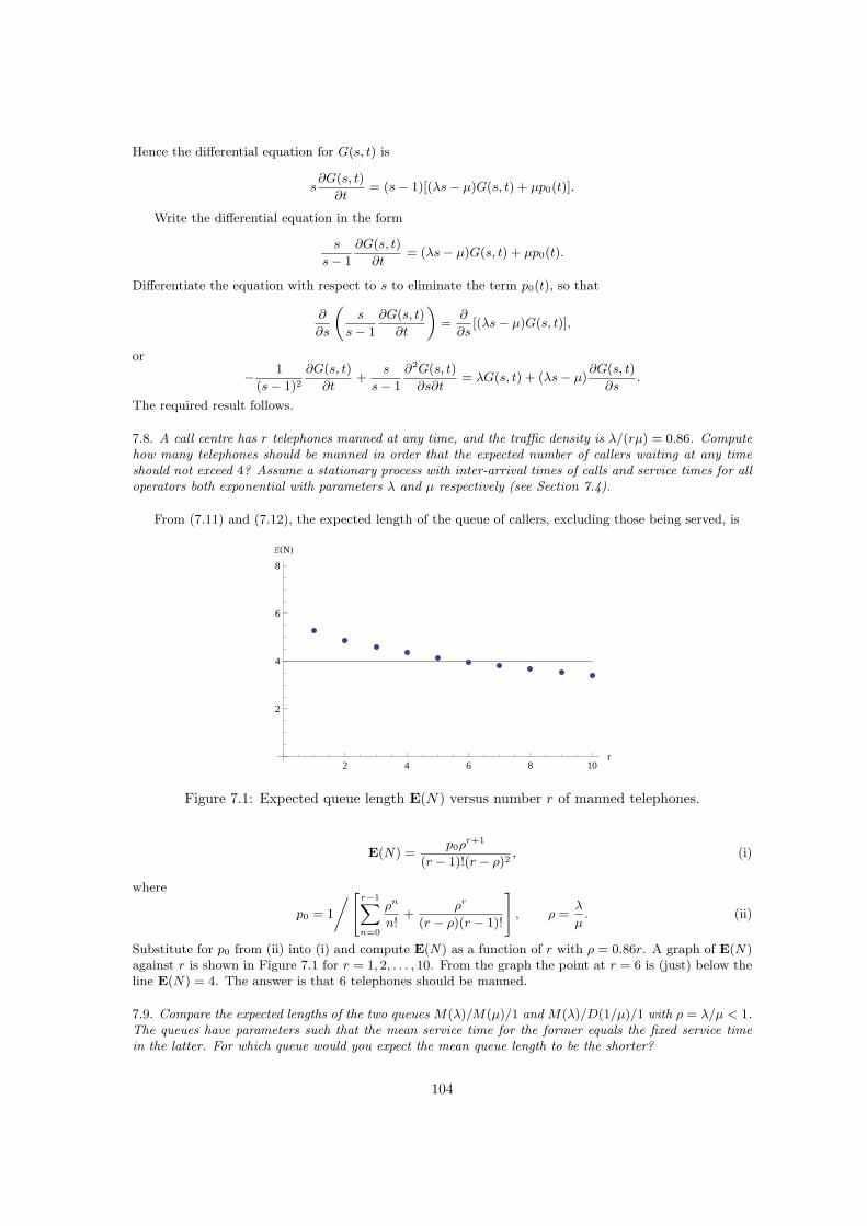
Hence the differential equation for G(s, t) is
s∂G(s, t)
∂t= (s− 1)[(λs− µ)G(s, t) + µp0(t)].
Write the differential equation in the form
s
s− 1
∂G(s, t)
∂t= (λs− µ)G(s, t) + µp0(t).
Differentiate the equation with respect to s to eliminate the term p0(t), so that
∂
∂s
(s
s− 1
∂G(s, t)
∂t
)=
∂
∂s[(λs− µ)G(s, t)],
or
− 1
(s− 1)2∂G(s, t)
∂t+
s
s− 1
∂2G(s, t)
∂s∂t= λG(s, t) + (λs− µ)
∂G(s, t)
∂s.
The required result follows.
7.8. A call centre has r telephones manned at any time, and the traffic density is λ/(rµ) = 0.86. Computehow many telephones should be manned in order that the expected number of callers waiting at any timeshould not exceed 4? Assume a stationary process with inter-arrival times of calls and service times for alloperators both exponential with parameters λ and µ respectively (see Section 7.4).
From (7.11) and (7.12), the expected length of the queue of callers, excluding those being served, is
2 4 6 8 10r
2
4
6
8
EHNL
Figure 7.1: Expected queue length E(N) versus number r of manned telephones.
E(N) =p0ρ
r+1
(r − 1)!(r − ρ)2, (i)
where
p0 = 1
/[r−1∑n=0
ρn
n!+
ρr
(r − ρ)(r − 1)!
], ρ =
λ
µ. (ii)
Substitute for p0 from (ii) into (i) and compute E(N) as a function of r with ρ = 0.86r. A graph of E(N)against r is shown in Figure 7.1 for r = 1, 2, . . . , 10. From the graph the point at r = 6 is (just) below theline E(N) = 4. The answer is that 6 telephones should be manned.
7.9. Compare the expected lengths of the two queues M(λ)/M(µ)/1 and M(λ)/D(1/µ)/1 with ρ = λ/µ < 1.The queues have parameters such that the mean service time for the former equals the fixed service timein the latter. For which queue would you expect the mean queue length to be the shorter?
104
From Section 7.3(b), the expected length of the M(λ)/M(µ)/1 queue is, with ρ = λ/µ < 1,
E1(N) =ρ
1− ρ.
Since λτ = λ/µ = ρ (τ is the fixed service time), the expected length of the M(λ)/D(1/µ)/1 is (see end ofSection 7.5)
E2(N) =ρ(1− 1
2ρ)
1− ρ.
It follows that
E2(N) =ρ
1− ρ−
12ρ2
1− ρ≤ ρ
1− ρ= E1.
In this case the queue with fixed service time has the shorter expected length.
7.10. A queue is serviced by r servers, with the distribution of the inter-arrival times for the queue beingexponential with parameter λ and each server has a common exponential service time distribution withparameter µ. If N is the random variable for the length of the queue including those being served, showthat its expected value is
E(N) = p0
[r−1∑n=1
ρn
(n− 1)!+
ρr[r2 + ρ(1− r)]
(r − 1)!(r − ρ)2
],
where ρ = λ/µ < r, and
p0 = 1
/[r−1∑n=0
ρn
n!+
ρr
(r − ρ)(r − 1)!
].
(see equation (7.11)).If r = 2, show that
E(N) =4ρ
4− ρ2.
For what interval of values of ρ is the expected length of the queue less than the number of servers?
For the M(λ)/M(µ)/r queue, the probability that there n persons in the queue is
pn =
{ρnp0/n! n < rρnp0/(rn−rr!) n ≥ r
,
where p0 is given in the question. The expected length of the queue including those being served is
E(N) =
∞∑n=1
npn = p0
[r−1∑n=1
nρn
n!+
∞∑n=r
nρn
rn−rr!
]= p0
[r−1∑n=1
ρn
(n− 1)!+
rr
r!
∞∑n=r
n(
ρ
r
)n
].
Consider the series
R =
∞∑n=r
n(
ρ
r
)n
.
Using the method for summing geometric series twice
R =(
ρ
r
)r r(r2 + ρ− ρr)
(r − ρ)2.
Hence
E(N) = p0
[r−1∑n=1
ρn
(n− 1)!+
ρr[r2 + ρ(1− r)]
(r − 1)!(r − ρ)2
],
as required.If r = 2 (two servers) then
p0 = 1
/[1 + ρ +
ρ2
(2− ρ)
]=
2− ρ
2 + ρ,
105
and
E(N) = p0
[ρ +
ρ2(4− ρ)
(2− ρ)2
]=
4ρ
4− ρ2.
The expected length of the queue is less than the number of servers if
4ρ
4− ρ2< 2, or ρ2 + 2ρ− 4 < 0.
The roots of ρ2 + 2ρ− 4 = 0 are ρ = −1±√5. The required range for ρ is 0 < ρ <√
5− 1.
7.11. For a queue with two servers, the probability pn that there are n servers in the queue, including thosebeing served, is given by
p0 =2− ρ
2 + ρ, p1 = ρp0, pn = 2
(ρ
2
)n
p0, (n ≥ 2),
where ρ = λ/µ (see Section 7.4). If the random variable X is the number of people in the queue, find itsprobability generating function. Hence find the mean length of the queue including those being served.
The probability generating function for this queue with two servers is, summing the geometric series,
G(s) = p0 + p0ρs + 2p0
∞∑n=2
(ρ
2
)n
sn =
(2− ρ
2 + ρ
)[1 + ρs +
ρ2s2
2− ρs
]
=
(2− ρ
2 + ρ
)(2 + ρs
2− ρs
),
assuming that 0 ≤ ρs < 2.For the mean we require
G′(s) =
(2− ρ
2 + ρ
)4ρ
(2− ρs)2.
Then the mean length of the queue
µ = G′(1) =4ρ
(4− ρ2),
which agrees with the result from Problem 7.10.
7.12. The queue M(λ)/D(τ)/1, which has a fixed service time of duration τ for every customer, has theprobability generating function
G(s) =(1− ρ)(1− s)
1− seρ(1−s),
where ρ = λτ (0 < ρ < 1) (see Section 7.5).(a) Find the probabilities p0, p1, p2.(b) Find the expected value and variance of the length of the queue.(c) Customers are allowed a service time τ which is such that the expected length of the queue is twoindividuals. Find the value of the traffic density ρ.
(a) The Taylor series for G(s) is
G(s) = (1− ρ) + (1− ρ)(eρ − 1)s + (1− ρ)(eρ − ρ− 1)eρs2 + O(s3).
Hencep0 = 1− ρ, p1 = (1− ρ)(eρ − 1), p2 = (1− ρ)(eρ − ρ− 1)eρ.
(b) The first two derivatives of G(s) are
G′(s) =esρ(−1 + ρ)
(esρ + eρ
(−1 + sρ− s2ρ
))
(esρ − eρs)2,
106
G′′(s) =eρ+sρ(−1 + ρ)
(esρ
(2 + (2− 4s)ρ + (−1 + s)sρ2
)+ eρ
(−2 + 2sρ− s2ρ2 + s3ρ2
))
(esρ − eρs)3.
It follows that the mean and variance are
E(N) = G′(1) =ρ(2− ρ)
2(1− ρ),
V(N) = G′′(1) + G′(1)− [G′(1)]2 =ρ
12(1− ρ)2(12− 18ρ + 10ρ2 − ρ3).
(c) We require G′(1) = 2, or 2 − 2ρ = ρ − 12ρ2. Hence ρ2 − 6ρ + 4 = 0. The roots of this quadratic
equation are ρ = λτ = 3±√5: the density is ρ = 3 +√
5 since ρ must be less than 1.
7.13. For the baulked queue which has a maximum length of m beyond which customers are turned away,The probabilities that there are n individuals in the queue are given by
pn =ρn(1− ρ)
1− ρm+1, (0 < ρ < 1), pn =
1
m + 1(ρ = 1),
for n = 0, 1, 2, . . . , m. Show that the probability generating functions are
G(s) =(1− ρ)[1− (ρs)m+1]
(1− ρm+1)(1− ρs), (ρ 6= 1),
and
G(s) =1− sm+1
(m + 1)(1− s), (ρ = 1).
Find the expected value of the queue length including the person being served.
The probability generating function G(s) of the baulked queue is defined by, for ρ 6= 1,
G(s) =
m∑n=0
pnsn =
(1− ρ
1− ρm+1
) m∑n=0
ρnsn =(1− ρ)(1− ρm+1sm+1)
(1− ρm+1)(1− ρs),
using the formula for the sum of the geometric series. The first derivative of G(s) is
G′(s) =(1− ρ)ρ (1− (sρ)m −m(sρ)m(1− sρ))
(1− sρ)2 (1− ρ1+m).
The expected length of the queue is
E(N) = G′(1) =ρ
1− ρ− (1 + m)ρ1+m
1− ρ1+m
If ρ = 1, then
G(s) =
∞∑n=0
pnsn =1
m + 1
m∑n=0
sn =1− sm+1
(m + 1)(1− s).
Its first derivative is
G′(s) =1− (1 + m)sm + ms1+m
(1 + m)(1− s)2.
The expected length of the queue is E(N) = G′(1) = 12m.
7.14. In Section 7.3(ii), the expected length of the queue with parameters λ and µ, including the personbeing served was shown to be ρ/(1−ρ). What is the expected length of the queue excluding the person beingserved?
107
The expected length of the queue excluding the person being served is given by
E(N) =
∞∑n=2
(n− 1)pn =
∞∑n=2
(n− 1)(ρn − ρn+1)
=
∞∑n=2
nρn −∞∑
n=2
ρn −∞∑
n=3
nρn + 2
∞∑n=3
ρn
= 2ρ2 − ρ2
1− ρ+
2ρ3
1− ρ
=ρ2
1− ρ
7.15. An M(λ)/M(µ)/1 queue is observed over a long period of time. Regular sampling indicates that themean length of the queue including the person being served is 3, whilst the mean waiting time to completionof service by any customer arriving is 10 minutes. What is the mean service time?
From Section 7.3, the mean length of the queue is 3, and the mean time to service is 10 minutes: hence
ρ
1− ρ= 3,
ρ
µ(1− ρ)= 10.
Hence
ρ =3
4and µ =
ρ
10(1− ρ)=
3
10.
7.16. An M(λ)/G/1 queue has a service time with a gamma distribution with parameters n and α wheren is a positive integer. The density function of the gamma distribution is
f(t) =αntn−1e−αt
(n− 1)!, t > 0.
Show that, assuming ρ = λn/α, the expected length of the queue including the person being served is givenby
ρ[2n− (n− 1)ρ]
2n(1− ρ)].
The formula for the expected length of queue is given by (7.25):
E(X) =2ρ− ρ2 + λ2V(S)
2(1− ρ),
where ρ = λE(S), and S is the random variable of the service time. Since S has a gamma distributionwith parameters n and α, then
E(S) =n
α, V(S) =
n
α2, ρ = λE(S) =
λn
α.
Hence
E(X) =2λnα− λ2n2 + λ2n
2α(α− λn).
This result assumes λ < α/n.
7.17. The service in a single-server queue must take at least 2 minutes and must not exceed 8 minutes, andthe probability that the service is completed at any time between these times is uniformly distributed overthe time interval. The average time between arrival is 4 minutes, and the arrival distribution is assumedto be exponential. Calculate expected length of the queue.
108

The density of the uniform distribution is
f(t) =
{1/(τ2 − τ1) τ1 ≤ t ≤ τ2
0 elsewhere
The expected length of the queue is given by (7.25). In this formula, we require E(S) and V(S). They aregiven by
E(S) =
∫ ∞
−∞tf(t)dt =
∫ τ2
τ1
tdt
τ2 − τ1=
1
2(τ2 + τ1).
By (7.21), it follows that the traffic density is ρ = λE(S) = 12λ(τ2 − τ1). The variance is given by
V(S) = E(S2)− [E(S)]2 =
∫ τ2
τ1
t2dt
τ2 − τ1− 1
4(τ2 − τ1)
2
=1
3(τ2
2 + τ1τ2 + τ21 )− 1
4(τ2 + τ1)
2
=1
12(τ2 − τ1)
2 =ρ2
3λ2
The formula is simpler if (7.25) is expressed as a function of the traffic density ρ. Thus, substitutingfor V(S), the expected queue length is for ρ < 1,
E(X) =2ρ− ρ2 + λ2V(S)
2(1− ρ)=
2ρ− ρ2 + 13ρ2
2(1− ρ)=
ρ(3− ρ)
3(1− ρ). (i)
In the particular case τ2 − τ1 = 4 minutes. Hence the expected time between arrivals is∫ ∞
0
λte−λtdt =1
λ.
Hence λ = 14
(minutes)−1. Since τ2 − τ1 = 6 minutes, then ρ = 12· 1
4· 6 = 3
4. Finally, the expected length
in eqn (i) becomes
E(X) =34(1− 3
4)
3(1− 34)
=9
4.
7.18. A person arrives at an M(λ)/M(µ)/1 queue. If there are two people in the queue (excluding customersbeing served) the customer goes away and does not return. If there are there are fewer than two queueingthen the customer joins the queue. Find the expected waiting time for the customer to the start of service.
This a is a baulked queue with baulking after 2 customers in the queue but not being served. Themethod is similar to that in Section 7.3(c). Let Ti, (i = 1, 2) be the random variable representing the timefor customer i to reach the service position. Let S1 and S2 be the random variables defined by
S1 = T1, S2 = T1 + T2.
As explained in Section 7.3(c), the densities of S1 and S2 are gamma with parameters respectively µ, 1and µ, 2, are
f1(t) = µe−µt (t > 0), f2(t) = µ2te−µt, (t > 0). (i)
From Example 7.1, the probability that there are n persons in the queue is
pn =ρn(1− ρ)
1− ρ3, (n = 0, 1, 2). (ii)
Then, using (i) and (ii)
P(S1 + S2 > T ) = P(S1 > t)p1 + P(S2 > t)p2
=ρ(1− ρ)
1− ρ3
∫ ∞
t
f1(s)ds +ρ2(1− ρ)
1− ρ3
∫ ∞
t
f2(s)ds
=ρ(1− ρ)
1− ρ3
[∫ ∞
t
µe−µsds + ρ
∫ ∞
t
µ2se−µsds
]
=ρ(1− ρ)
1− ρ3e−µt[1 + ρµt + ρ].
109
The density associated with this probability is
g(t) =d
dt
[1− ρ(1− ρ)
1− ρ3e−µt[1 + ρµt + ρ]
]=
ρ(1− ρ)
1− ρ3µ(1 + ρµt)e−µt.
Finally, the expected waiting time for the customer to start service is
E(S1 + S2) =
∫ ∞
0
tg(t)dt =ρ(1− ρ)µ
1− ρ3
∫ ∞
0
(t + ρµt2)e−µtdt =ρ(1− ρ)(1 + 2ρ)
1− ρ3=
ρ(1 + 2ρ)
1 + ρ + ρ2
7.19. A customer waits for service in a bank in which there are four counters with customers at each counterbut otherwise no one is queueing. If the service time distribution is negative exponential with parameter µfor each counter, for how long should the queueing customer have to wait on average?
For each till, the density is f(t) = µe−µt. The corresponding probability function is
F (t) =
∫ t
0
f(s)ds =
∫ t
0
µe−µsds = 1− e−µt.
Let T be random variable of the time to complete service at any till. Then the probability that T is greaterthan time t is
P(T > t) = P(T > t for till 1)P(T > t for till 2)P(T > t for till 3)P(T > t for till 4)
= e−µte−µte−µte−µt = e−4µt.
Hence the density of T is g(t) = 4µe−4µt (t > 0), which is exponential with parameter 4µ. The mean timefor a till becoming available is
E(T ) =
∫ ∞
0
4µte−4µtdt =1
4µ,
after integrating by parts.
7.20. A hospital has a waiting list for two operating theatres dedicated to a particular group of operations.Assuming that the queue is stationary, and that the waiting list and operating time can be viewed as anM(λ)/M(µ)/1 queue, show that the expected value of the random variable N representing the length of thequeue is given by
E(N) =ρ3
4− ρ2, ρ =
λ
µ< 2.
The waiting list is very long at 100 individuals. Why will ρ be very close to 2? Put ρ = 2 − ε whereε > 0 is small. Show that ε ≈ 0.02. A third operating theatre is brought into use with the same operatingparameter µ. What effect will this new theatre have on the waiting list eventually?
In Section 7.4, apply eqns (7.11) and (7.12) (in the book) with r = 2 giving for the expected length ofthe queue of patients as
E(N) =p0ρ
3
(2− ρ)2,
where
p0 = 1
/[1 + ρ +
ρ2
2− ρ
]=
2− ρ
2 + ρ.
Elimination of p0 between these equations leads to
E(N) =ρ3
4− ρ2, λ < 2.
For E(N) to be large, 4− ρ2 is small. Since 0 < ρ < 2, let ρ = 2− ε with ε small. Then
E(N) =2(1− 1
2ε)
ε(1− 14ε)
=1
ε+ O(1).
110
as ε → 0. If E(N), then ε ≈ 2/100 = 0.02.If r = 3 (which will require λ/µ < 3), then
E(N) =p0ρ
4
2(3− ρ)2,
where
p0 = 1
/[1 + ρ +
1
2ρ2 +
ρ3
2(3− ρ)
].
Therefore
E(N) =ρ4
(3− ρ)(6 + 4ρ + ρ2).
If ρ = 2− ε, then the expected length is
E(N) ≈ 8
9+ O(ε),
which is a significant reduction.
7.21. Consider the M(λ)/M(µ)/r queue which has r servers such that ρ = λ/µ < r. Adapting the methodfor the single-server queue (Section 7.3 (iii)), explain why the average service time for (n−r+1) customersto be served is (n− r + 1)/(µr) if n ≥ r. What is it if n < r? If n ≥ r, show that the average value of thewaiting time random variable T until service is
E(T ) =
∞∑n=r
n− r + 1
rµpn.
What is the average waiting time if service is included?
If n ≤ r− 1, then the arriving customer has immediate service. If n ≥ r, the customer must wait untiln−r+1 preceding customers have been served, and they take time (n−r+1)/(rµ) since the mean servicetime is 1/(rµ) for r servers. The expected value of the service time T until service is
E(T ) =
∞∑n=r
n− r + 1
rµpn,
where (see Section 7.4)
pn =ρnp0
rn−rr!, p0 = 1
/[r−1∑n=0
ρn
n!+
ρr
(r − ρ)(r − 1)!
].
Then
E(T ) =ρrp0
µrr!
∞∑n=r
(n− r + 1)(
ρ
r
)n−r
=ρrp0
µrr!
[1 + 2
(ρ
r
)+ 3
(ρ
r
)2
+ · · ·]
=ρrp0
µ(r − 1)!(r − ρ)2
The mean time represented by random variable T ′ until service is completed is
E(T ′) = E(T ) +1
µ.
7.22. Consider the queue M(λ)/M(µ)/r queue. Assuming that λ < rµ, what is the probability in the longterm that at any instant there is no one queueing excluding those being served?
111
The probability that no one is queueing is
qr = 1−∞∑
n=r
pn,
where (see Section 7.4) using the formula for the sum of a geometric series,
∞∑n=r
pn =p0r
r
r!
∞∑n=r
(ρ
r
)n
=p0ρ
r
(r − 1)!(r − ρ),
and
p0 = 1
/[r−1∑n=0
ρn
n!+
ρr
(r − ρ)(r − 1)!
].
7.23. Access to a toll road is controlled by a plaza of r toll booths. Vehicles approaching the toll boothschoose one at random: any toll booth is equally likely to be the one chosen irrespective of the number ofcars queueing (perhaps an unrealistic situation). The payment time is assumed to be negative exponentialwith parameter µ, and vehicles are assumed to approach as Poisson with parameter λ. Show that, viewedas a stationary process, the queue of vehicles at any toll booth is an M(λ/r)/M(µ)/1 queue assumingλ/(rµ) < 1. Find the expected number of vehicles queueing at any toll booth. How many cars would youexpect to be queueing over all booths?
One booth is out of action, and vehicles distribute themselves randomly over the remaining booths.Assuming that λ/[(r − 1)µ] < 1, how many extra vehicles can be expected to be queueing overall?
It is assumed to be an M(λ/r/M(µ)/1) queue. For a random number Nn of cars at toll booth n(n = 1, 2, . . . r) is
E(Nn) =λ
µr − λ.
For all booths, the expected number of cars is
E(N1 + N2 + · · ·Nr) =rλ
µr − λ,
including cars at any booth.If one booth is out of action (say booth r) then the expected number of cars queueing is
E(N1 + N2 + · · ·Nr−1) =(r − 1)λ
µ(r − 1)− λ,
Hence the expected extra length of the queue is
(r − 1)λ
µ(r − 1)− λ− rλ
µr − λ=
λ2
[µ(rt− 1)− λ](µr − λ).
7.24. In an M(λ)/M(µ)/1 queue, it is decided that the service parameter µ should be adjusted to make themean length of the busy period 10 times the slack period to allow the server some respite. What should µbe in terms of λ?
From Section 7.3(d), in the stationary process, the expected length of the slack period is 1/λ and thatof the busy period 1/(µ− λ). Therefore the busy period is 10 times of the slack period if
1
µ− λ=
10
λ, or µ =
11
10λ.
7.25. In the baulked queue (see Example 7.1) not more than m ≥ 2 people (including the person beingserved) are allowed to form a queue, the arrivals having a Poisson distribution with parameter λ. If thereare m individuals in the queue, then any further arrivals are turned away. It is assumed that the service
112
distribution is exponential with rate µ. If ρ = λ/µ 6= 1, show that the expected length of the busy periods isgiven by (1− ρm)/(µ− λ).
For the baulked queue with a limit of m customers (including the person being served) the probabilitythat the queue is of length n is given by
pn =ρn(1− ρ)
1− ρn+1, (n = 0, 1, 2, . . . , m).
In the notation of Section 7.3(d) for slack and busy periods,
limj→∞
[1
j
j∑i=1
si
]=
1
λ,
and
limj→∞
[1
j
j∑i=1
bi
]=
1− p0
p0lim
j→∞
[1
j
j∑i=1
si
]=
1− p0
λp0=
1− ρm
µ− λ.
7.26. The M(λ)/D(τ)/1 queue has a fixed service time τ , and from Section 7.5, its probability generatingfunction is
G(s) =(1− λτ)(1− s)
1− seλτ(1−s).
Show that the expected length of its busy periods is τ/(1− λτ).
The average length of the slack periods is, in the notation of Section 7.3(d),
limj→∞
[1
j
j∑i=1
si
]=
1
λ,
since it depends on the arrival distribution. Also the average length of the busy periods is
limj→∞
[1
j
j∑i=1
bi
]=
1− p0
p0lim
j→∞
[1
j
j∑i=1
si
]=
1− p0
p0λ.
From the given generating function p0 = G(0) = 1− λτ , so that the average length of busy periods is
limj→∞
[1
j
j∑i=1
bi
]=
τ
1− λτ.
7.27. A certain process has the (r+1) states En, (n = 0, 1, 2, . . . r). The transition rates between state n andstate n+1 is λn = (r−n)λ, (n = 0, 1, 2, . . . , r− 1), and between n and n− 1 is µn = nµ, (n = 1, 2, . . . , r).These are the only possible transitions at each step in the process. [This could be interpreted as a ‘capped’birth and death process in which the population size cannot exceed r.]
Find the differential-difference equation for the probabilities pn(t), (n = 0, 1, 2, . . . , r), that the process isin state n at time t. Consider the corresponding staionary process in which dpn/dt →∞0 and pn(t) → pn
as t →∞. Show that
pn =
(λ
µ
)n (r
n
)µr
(λ + µ)r, (n = 0, 1, 2, . . . , r).
In (6.25), let
λn = (r − n)λ, (n = 0, 1, 2, . . . , r − 1), µn = nµ, (n = 1, 2, . . . , r),
113
so that the finite system of differential-difference equations are
p′0(t) = λrp0(t) + µp1(t),
p′n(t) = (r − n + 1)λpn−1(t)− [(r − n) + nµ]pn(t) + (n + 1)µpn+1(t), (n = 1, 2, . . . , r − 1),
p′r(t) = λpr−1(t)− rµpr(t).
The time-independent stationary process satisfies the difference equations
λrp0 + µp1 = 0,
(r − n + 1)λpn−1 − [(r − n) + nµ]pn + (n + 1)µpn+1 = 0, (n = 1, 2, . . . , r − 1),
λpr−1 − rµpr = 0.
Let un = λ(r − n)pn − (n + 1)µpn+1. The the difference equations become
u0 = 0, un−1 − un = 0, (n = 1, 2, . . . , r − 1), ur−1 = 0.
We conclude that un = 0 for (n = 0, 1, 2, . . . , r − 1). Hence
pn+1 =λ
µ
(r − n
n + 1
)pn.
Repeated application of this formula gives
pn =
(λ
µ
)nr(r + 1) · · · (r − n + 1)
n!p0 =
(λ
µ
)n (r
n
)p0, (n = 0, 1, 2, . . . , r).
The probability p0 is defined by
1 =
r∑n=0
pn =
r∑n=0
(λ
µ
)n (r
n
)p0 = p0
(1 +
λ
µ
)r
.
Hence
p0 =µr
(λ + µ)r,
so that, finally
pn =
(λ
µ
)n (r
n
)µr
(λ + µ)r.
114
Chapter 8
Reliability and renewal
8.1. The lifetime of a component has a uniform density function given by
f(t) =
{1/(t1 − t0) 0 < t0 < t < t10 otherwise
For all t > 0, obtain the reliability function R(t) and the failure rate function r(t) for the component.Obtain the expected life of the component.
For the given density, the distribution function is
F (t) =
{0 0 ≤ t ≤ t0(t− t0)/(t1 − t0) t0 < t < t11 t ≥ t1
Therefore the reliability function R(t) is
R(t) = 1− F (t) =
{1 0 ≤ t ≤ t0(t1 − t)/(t1 − t0) t0 < t < t10 t ≥ t1
,
and the failure rate function r(t) is
r(t) =f(t)
R(t)=
{0 0 ≤ t ≤ t01/(t1 − t) t0 < t < t1does not exist t ≥ t1
.
Failure of the component will not occur for 0 ≤ t ≤ t0 since R(t) = 1 in this interval. The component willnot survive beyond t = t1.
If T is a random variable of the lifetime of the component, then the expected lifetime is given by
E(T ) =
∫ ∞
0
tf(t)dt =
∫ t1
t0
tdt
t1 − t0=
t21 − t202(t1 − t0)
=1
2(t0 + t1).
8.2. Find the reliability function R(t) and the failure rate function r(t) for the gamma density
f(t) = λ2te−λt, t > 0.
How does r(t) behave for large t? Find the mean and variance of the time to failure.
For the given gamma density,
F (t) = λ2
∫ t
0
se−λsds = 1− e−λt(1 + λt).
115
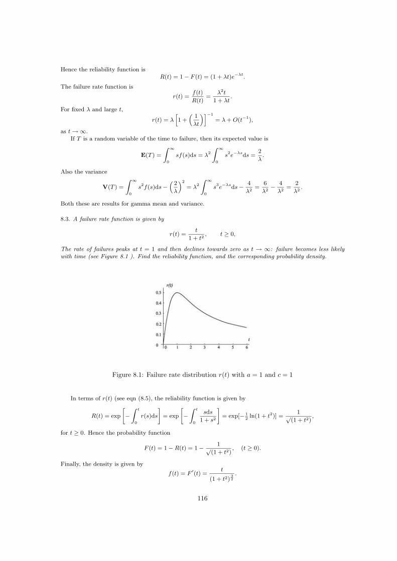
Hence the reliability function isR(t) = 1− F (t) = (1 + λt)e−λt.
The failure rate function is
r(t) =f(t)
R(t)=
λ2t
1 + λt.
For fixed λ and large t,
r(t) = λ[1 +
(1
λt
)]−1
= λ + O(t−1),
as t →∞.If T is a random variable of the time to failure, then its expected value is
E(T ) =
∫ ∞
0
sf(s)ds = λ2
∫ ∞
0
s2e−λsds =2
λ.
Also the variance
V(T ) =
∫ ∞
0
s2f(s)ds−(
2
λ
)2
= λ2
∫ ∞
0
s3e−λsds− 4
λ2=
6
λ2− 4
λ2=
2
λ2.
Both these are results for gamma mean and variance.
8.3. A failure rate function is given by
r(t) =t
1 + t2, t ≥ 0,
The rate of failures peaks at t = 1 and then declines towards zero as t → ∞: failure becomes less likelywith time (see Figure 8.1 ). Find the reliability function, and the corresponding probability density.
Figure 8.1: Failure rate distribution r(t) with a = 1 and c = 1
In terms of r(t) (see eqn (8.5), the reliability function is given by
R(t) = exp
[−
∫ t
0
r(s)ds
]= exp
[−
∫ t
0
sds
1 + s2
]= exp[− 1
2ln(1 + t2)] =
1√(1 + t2)
,
for t ≥ 0. Hence the probability function
F (t) = 1−R(t) = 1− 1√(1 + t2)
, (t ≥ 0).
Finally, the density is given by
f(t) = F ′(t) =t
(1 + t2)32
.
116
8.4. A piece of office equipment has a piecewise failure rate function given by
r(t) =
{2λ1t, 0 < t ≤ t0,2(λ1 − λ2)t0 + 2λ2t, t > t0
λ1, λ2 > 0.
Find its reliability function.
The reliability function is given by
R(t) = exp
[−
∫ t
0
r(s)ds
],
where, for 0 < t ≤ t0, ∫ t
0
r(s)ds = 2λ1
∫ t
0
sds = λ1t2,
and, for t > t0,∫ t
0
r(s)ds =
∫ t0
0
r(s)ds +
∫ t
t0
r(s)ds
= λ1t20 +
∫ t
t0
[2(λ1 − λ2)t0 + 2λ2s]ds
= λ1t20 + 2(λ1 − λ2)t0(t− t0)] + λ2(t
2 − t20)
= t0(λ1 − λ2)(2t− t0) + λ2t2
Hence the reliability function is
R(t) =
{e−λ1t2 0 < t ≤ t0
e−[t0(λ1−λ2)(2t−t0)+λ2t2] t > t0.
8.5. A laser printer is observed to have a failure rate function r(t) = 2λt (t > 0) per hour whilst in use,where λ = 0.00021(hours)−2: r(t) is a measure of the probability of the printer failing in any hour giventhat it was operational at the beginning of the hour. What is the probability that the printer is workingafter 40 hours of use? Find the probability density function for the time to failure. What is the expectedtime before the printer will need maintenance?
Since r(t) = 2λt, the reliability function is
R(t) = exp
[−2λ
∫ t
0
sds
]= e−λt2 .
Hence R(40) = e−0.00021×40×40 = 0.715. The probability of that the printer is working after 40 hours is
0.715. The probability of failure is F (t)1−R(t), so that F (t) = 1− e−λt2 .By (8.8), the expected time T of the random variable to failure is
E(T ) =
∫ ∞
0
R(t)dt =
∫ ∞
0
e−λt2dt =1
2
√π
λ= 61.2 hours,
(see the Appendix for the value of the integral).
8.6. The time to failure is assumed to be gamma with parameters α and n, that is,
f(t) =α(αt)n−1e−αt
(n− 1)!, t > 0.
Show that the reliability function is given by
R(t) = e−αt
n−1∑r=0
αrtr
r!.
117
Find the failure rate function and show that limt→∞ r(t) = α. What is the expected time to failure?
The gamma distribution function is
F (t, α, n) =
∫ t
0
α(αs)n−1e−αs
(n− 1)!ds =
αn
(n− 1)!
∫ t
0
sn−1e−αsds
= − αn−1
(n− 1)!tn−1e−αt +
αn−1
(n− 2)!F (t, α, n− 1)
= e−αt
[−αn−1tn−1
(n− 1)!− αn−2tn−2
(n− 2)!− · · · − αt
1!
]+
∫ t
0
e−αsds
= 1− e−αt
n−1∑r=0
αrtr
r!.
after repeated integration by parts. The reliability function is therefore
R(t) = 1− F (t, α, n) = e−αt
n−1∑r=0
αrtr
r!.
The failure rate function r(t) is defined by
r(t) =f(t)
R(t(=
α(αt)n−1e−αt
(n− 1)!
/[e−αt
n−1∑r=0
αrtr
r!
]
= αntn−1
/[(n− 1)!
n−1∑r=0
αrtr
r!
]
For the limit, express r(t) in the form
r(t) = αn
/[(n− 1)!
n−1∑r=0
αrtr−n+1
r!
]→ αn
/[(n− 1)!
αn−1
(n− 1)!
]= α
as t →∞.The expected time to failure is
E(T ) =
∫ ∞
0
αntne−αtdt
(n− 1)!=
αn
(n− 1)!· n!
αn+1=
n
α.
8.7. A electrical generator has an exponentially distributed failure time with parameter λf and the subse-quent repair time is exponentially distributed with parameter λr. The generator is started up at time t = 0.What is the mean time for generator to fail and the mean time from t = 0 for it to be operational again?
As in Section 8.4, the mean time to failure is 1/λf . The mean repair time is 1/λr, so that the meantime to the restart is
1
λf+
1
λr.
8.8. A hospital takes a grid supply of electricity which has a constant failure rate λ. This supply is backedup by a stand-by generator which has a gamma distributed failure time with parameters (2, µ). Find thereliability function R(t) for the whole electricity supply. Assuming that time is measured in hours, whatshould the relation between the parameters λ and µ be in order that R(1000)=0.999?
For the grid supply, the reliability function is Rg(t) = e−λt. For the stand-by supply, the reliabilityfunction is (see Problem 8.6)
Rs(t) = e−µt
1∑r=0
µrtr
r!= e−µt(1 + µt).
118
The reliability function for the system is
R = 1− [1−Rg(t)][1−Rs(t)] = 1− [1− e−λt][1− (1 + µt)e−µt]
= e−λt − (1 + µt)e−(λ+µ)t + (1 + µt)e−µt.
Let T = 1000 hours. Then solving the equation above for λ at time t = T , we have
λ = − 1
Tln
[R(T )− (1 + µT )e−µT
1− (1 + µT )e−µT
],
where R(T ) = R(1000) = 0.999.
8.9. The components in a renewal process with instant renewal are identical with constant failure rateλ = (1/50)(hours)−1. If the system has one spare component which can take over when the first fails, findthe probability that the system is operational for at least 24 hours. How many spares should be carried toensure that continuous operation for 24 hours occurs with probability 0.98?
Let T1 and T2 be respectively random variables of the times to failure of the components. Let S2 bethe time to failure of these components. If τ = 24 hours is the operational time to be considered, then, asin Example 8.5,
P(S2 < τ) = 1− (1 + λτ)e−λτ.
Hence
P(S2 < 24) = 1−(1 +
24
50
)e−24/50 = 1− 0.916.
The required probability is 0.916.This is the reverse problem: given the probability, we have to compute n. If Sn is the time to failure,
then
P(SN < τ) = Fn(τ) =
∫ τ
0
fn(s)ds =λn
(n− 1)!
∫ τ
0
sn−1e−λsds
= 1− e−λτ
[1 + λτ +
(λτ)2
2!+ · · ·+ (λτ)n−1
(n− 1)!
]
The smallest value of n is required which makes 1− Fn(24) > 0.98. Conputation gives
1− F2(24) = 0.916, F3(24) = 0.987 > 0.98.
Three components are required.
8.10. A device contains two components c1 and c2 with independent failure times T1 and T2 from timet = 0. If the densities of the times to failure are f1 and f2 with probability distributions F1 and F2, showthat the probability that c1 fails before c2 is given by
P{T1 < T2} =
∫ ∞
y=0
∫ y
x=0
f1(x)f2(y)dxdy, =
∫ ∞
y=0
F1(y)f2(y)dy.
Find the probability P{T1 < T2} in the cases:(a) both failure times are exponentially distributed with parameters λ1 and λ2;(b) both failure times have gamma distributions with parameters (2, λ1) and (2, λ2).
The probability that c1 fails befors c2 is
P(T1 < T2) =
∫ ∫
A
f1(x)f2(x)dx,
where the region A is shown in Figure 8.2. As a repeated integral the double integral can be expressed as
P(T1 < T2) =
∫ ∞
0
∫ y
0
f1(x)f2(y)dxdy =
∫ ∞
0
[F1(y)− F1(0)]f2(y)dy =
∫ ∞
0
F1(y)f2(y)dy,
119
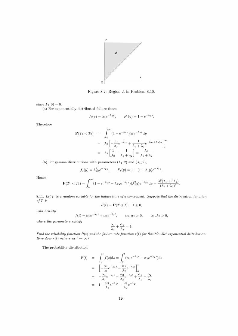
A
O
y
x
Figure 8.2: Region A in Problem 8.10.
since F1(0) = 0.(a) For exponentially distributed failure times
f2(y) = λ2e−λ2y, F1(y) = 1− e−λ1y.
Therefore
P(T1 < T2) =
∫ ∞
0
(1− e−λ1y)λ2e−λ2ydy
= λ2
[− 1
λ2e−λ2y +
1
λ1 + λ2e−(λ1+λ2)y
]∞0
= λ2
[1
λ2− 1
λ1 + λ2
]=
λ1
λ1 + λ2
(b) For gamma distributions with parameters (λ1, 2) and (λ1, 2),
f2(y) = λ22ye−λ2y, F1(y) = 1− (1 + λ1y)e−λ1y.
Hence
P(T1 < T2) =
∫ ∞
0
(1− e−λ1y − λ1ye−λ1y)(λ22y)e−λ2ydy =
λ21(λ1 + 3λ2)
(λ1 + λ2)3.
8.11. Let T be a random variable for the failure time of a component. Suppose that the distribution functionof T is
F (t) = P(T ≤ t), t ≥ 0,
with densityf(t) = α1e
−λ1t + α2e−λ2t, α1, α2 > 0, λ1, λ2 > 0,
where the parameters satisfyα1
λ1+
α2
λ2= 1.
Find the reliability function R(t) and the failure rate function r(t) for this ‘double’ exponential distribution.How does r(t) behave as t →∞?
The probability distribution
F (t) =
∫ t
0
f(s)ds =
∫ t
0
(α1e−λ1s + α2e
−λ2s)ds
=[−α1
λ1e−λ1s − α2
λ2e−λ2s
]t
0
= −α1
λ1e−λ1t − α2
λ2e−λ2t +
α1
λ1+
α2
λ2
= 1− α1
λ1e−λ1t − α2
λ2e−λ2t
120
The reliability function is therefore
R(t) = 1− F (t) =α1
λ1e−λ1t +
α2
λ2e−λ2t.
The failure rate function is
r(t) =f(t)
R(t)=
(α1e
−λ1t + α2e−λ2t
)/(α1
λ1e−λ1t +
α2
λ2e−λ2t
).
As t →∞,
r(t) →{
λ1 if λ2 > λ1
λ2 if λ2 < λ1
λ if λ1 = λ2 = λ
8.12. The lifetimes of components in a renewal process with instant renewal are identically distributed withconstant failure rate λ. Find the probability that at least three components have been replaced by time t.
In the notation of Section 8.7
P(S3 < t) = F3(t) =
∫ t
0
F2(t− y)f(y)dy,
whereF2(t) = 1− (1 + λt)e−λt, f(t) = λe−λt.
Then
P(S3 ≤ t) =
∫ t
0
[1− (1 + λ(t− y)e−λ(t−y)]λe−λydy
= 1− (1 + tλ + 12t2λ2)e−λt.
8.13. The lifetimes of components in a renewal process with instant renewal are identically distributed witha failure rate which has a uniform distribution with density
f(t) =
{1/k 0 < t < k0 elsewhere
Find the probability that at least two components have been replaced at time t.
For the uniform density
F1(t) =
{0 t < 0t/k 0 < t < k1 t > k
As in Example 8.5,
F2(t) =
∫ t
0
F1(t− y)F (y)dy.
Interval 0 < t < k.
F2(t) =1
k
∫ t
0
F1(t− y)dy =1
k2
∫ t
0
(t− y)dy =t2
2k2.
Interval t > k
F2(t) =1
k
∫ k
0
F2(t− y)dy =1
k2
∫ k
t−k
(t− y)dy
=1
k2[− 1
2(t− k)2 + 1
2k2]
=t
2k2(2k − t)
121
To summarize
F2(t) =
{t2/(2k2) 0 < t < k
t(2k − t)/(2k2) t > k,
which is the probability that at least two components have failed.
8.14. The lifetimes of components in a renewal process with instant renewal are identically distributed eachwith reliability function
R(t) =1
2(e−λt + e−2λt), t ≥ 0, λ > 0.
Find the probability that at least two components have been replaced by time t.
Given the reliability function, it follows that the distribution function and its density are given by
F (t) = 1−R(t) = 1− 12e−λt − 1
2e−2λt,
f(t) = F ′(t) = 12[λe−λt + 2λe−2λt].
In the notation of Example 8.5,
P(S2 < t) = F2(t) =
∫ t
0
F (t− s)f(s)ds
=1
2
∫ t
0
[1− 12e−λ(t−s) − 1
2e−2λ(t−s)][λe−λs + 2λe−2λt]ds
=1
4[4 + (1− 2λt)e−2λt − (5 + λt)e−λt],
which is the probability that at least two components have failed by time t.
8.15. The random variable T is the time to failure from t = 0 of a system. The distribution funmction forT is F (t), (t > 0). Suppose that the system is still functioning at time t = t0. Let Tt0 be the conditionaltime to failure from this time, and let Ft0(t) be its distribution function. Show that
Ft0(t) =F (t + t0)− F (t0)
1− F (t0), (t ≥ 0, t0 ≥ 0),
and that the mean of Tt0 is
E(Tt0) =1
1− F (t0)
∫ ∞
t0
[1− F (u)]du.
The distribution function for the conditional time to failure is
Ft0(t) = P(Tt0 ≤ t) = P(T − t0 ≤ t|T > t0)
=P(T − t0 ≤ t ∩ T > t0)
P(T > t0)(by eqn (1.2))
=P(t0 < T ≤ t + t0)
∂(T > t0)
=F (t + t0)− F (t0)
1− F (t0),
as required.For the mean
E(Tt0) =
∫ ∞
0
[1− F (t + t0)− F (t0)
1− F (t0)
]dt
=1
1− F (t0)
∫ ∞
0
[1− F (t + t0)]dt
=1
1− F (t0)
∫ ∞
t0
[1− F (u)]du, (where u = t + t0).
122
8.16. Suppose that the random variable T of the time to failure of a system has a uniform distribution fort > 0 given by
F (t) =
{t/t1, 0 ≤ t ≤ t1
1 t > t1.
Using the result from Problem 8.15, find the conditional probability function assuming that the system isstill working at time t = t0.
Thare are two cases to consider: t0 ≤ t1 and t0 > t1.• t0 ≤ t1. In the formula in Problem 8.15
F (t + t0) =
{(t + t0)/t1 0 ≤ t + t0 ≤ t1,1 t + t0 > t1
.
Hence
Ft0(t) =
[(t + t0)/t1]− [t0/t1]
1− [t0/t1]=
t
t1 − t00 ≤ t ≤ t1 − t0
1− [t0/t1]
1− [t0/t1]= 1 t > t1 − t0
.
• t0 > t1. Ft0 = P(T − t0 ≤ t|T > t0) = 1.
123
Chapter 9
Branching and other randomprocesses
9.1. In a branching process the probability that any individual has j descendants is given by
p0 = 0, pj =1
2j, (j ≥ 1).
Show that the probability generating function of the first generation is
G(s) =s
2− s.
Find the further generating functions G2(s), G3(s) and G4(s). Show by induction that
Gn(s) =s
2n − (2n − 1)s.
Find pn,j, the probability that the population size of the n-th generation is j given that the process startswith one individual. What is the mean population size of the n-th generation?
The generating function is given by
G(s) =
∞∑j=0
pjsj =
∞∑j=1
(s
2
)j
=s
2+
(s
2
)2
+ · · · = s
2− s,
using the geometric series formula for the sum.For the second generation G2(s) = G(G(s)), so that
G2(s) =s/(2− s)
2− [2/(2− s)]=
s
2(2− s)− s=
s
4− 3s.
Repeating this procedure,
G3(s) = G(G(G(s))) = G2(G(s)) =s
4(2− s)− 3s=
s
8− 7s,
G4(s) = G3(G(s)) =s
8(2− s)− 7s=
s
16− 15s.
Consider the formulaGn(s) =
s
2n − (2n − 1)s.
ThenGn+1(s) = G(Gn(s)) =
s
2n(2− s)− (2n − 1)s=
s
2n+1 − (2n+1 − 1)s.
124
Hence if the formula is correct for Gn(s) then it is true for Gn+1(s). The result has been verified for G2(s)and G3(s) so it is true for all n by induction on the integers.
Using the binomial expansion
Gn(s) =s
2n − (2n − 1)s=
s
2n
[1− (2n − 1)
2ns
]−1
=
∞∑j=1
(2n − 1
2n
)j−1
sj .
Hence the probability that the population size of the n-th generation is j is given by the coefficient of sj
in this series, namely
pn,j =(
2n − 1
2n
)j−1
.
Since G(s) = s/(2−s), then G′(s) = 2/(2−s)2, so that the mean of the first generation is µ = G′(1) = 2.Using result (9.7) in the text, the mean size of the n-th generation is
µn = G′n(1) = µn = 2n.
9.2. Suppose in a branching process that any individual has a probability given by the modified geometricdistribution
pj = (1− p)pj , (j = 0, 1, 2, . . .),
of producing j descendants in the next generation, where p (0 < p < 1) is a constant. Find the probabilitygenerating function of the second and third generations. What is the mean size of any generation?
The probability generating function is
G(s) =
∞∑j=0
pjsj =
∞∑j=0
(1− p)pjsj =1− p
1− ps,
using the formula for the sum of the geometric series.In the second generation
G2(s) = G(G(s)) =1− p
1− pG(s)=
1− p
1− p[(1− p)/(1− ps)]
=(1− p)(1− ps)
(1− p + p2)− ps,
and for the third generation
G3(s) = G2(G(s)) =(1− p)[1− {p(1− p)/(1− ps)}]
(1− p + p2)− {p(1− p)/(1− ps)}
=(1− p)(1− p + p2 − ps)
(1− 2p + 2p2)− p(1− p + p2)s
The mean size of the first generation is
µ = G′(1) =(1− p)p
(1− ps)2
∣∣∣∣s=1
=p
1− p.
From (9.7) in the book, it follows that µ2 = µ2, µ3 = µ3, and, in general, that µn = µn for the n-thgeneration.
9.3. A branching process has the probability generating function
G(s) = a + bs + (1− a− b)s2
for the descendants of any individual, where a and b satisfy the inequalities
0 < a < 1, b > 0, a + b < 1.
125
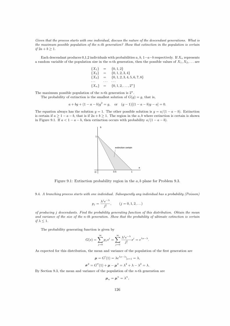
Given that the process starts with one individual, discuss the nature of the descendant generations. What isthe maximum possible population of the n-th generation? Show that extinction in the population is certainif 2a + b ≥ 1.
Each descendant produces 0,1,2 individuals with probabilities a, b, 1−a−b respectively. If Xn representsa random variable of the population size in the n-th generation, then the possible values of X1, X2, . . . are
{X1} = {0, 1, 2}{X2} = {0, 1, 2, 3, 4}{X3} = {0, 1, 2, 3, 4, 5, 6, 7, 8}· · · · · · · · ·{Xn} = {0, 1, 2, . . . , 2n}
The maximum possible population of the n-th generation is 2n.The probability of extinction is the smallest solution of G(g) = g, that is,
a + bg + (1− a− b)g2 = g, or (g − 1)[(1− a− b)g − a] = 0.
The equation always has the solution g = 1. The other possible solution is g = a/(1− a− b). Extinctionis certain if a ≥ 1− a− b, that is if 2a + b ≥ 1. The region in the a, b where extinction is certain is shownin Figure 9.1. If a < 1− a− b, then extinction occurs with probability a/(1− a− b).
a
b
1
O 10.5
extinction certain
Figure 9.1: Extinction probability region in the a, b plane for Problem 9.3.
9.4. A branching process starts with one individual. Subsequently any individual has a probability (Poisson)
pj =λje−λ
j!, (j = 0, 1, 2, . . .)
of producing j descendants. Find the probability generating function of this distribution. Obtain the meanand variance of the size of the n-th generation. Show that the probability of ultimate extinction is certainif λ ≤ 1.
The probability generating function is given by
G(s) =
∞∑j=0
pjsj =
∞∑j=0
λje−λ
j!sj = eλs−λ.
As expected for this distribution, the mean and variance of the population of the first generation are
µ = G′(1) = λeλs−λ|s=1 = λ,
σ2 = G′′(1) + µ− µ2 = λ2 + λ− λ2 = λ.
By Section 9.3, the mean and variance of the population of the n-th generation are
µn = µn = λn,
126
σ2n =
µn(σ2 − µ + µ2)(µn − 1)
µ(µ− 1)(λ 6= 1)
=λn+1(λn − 1)
λ− 1.
If λ = 1, then µn = 1 and σn = n.
9.5. A branching process starts with one individual. Any individual has a probability
pj =λ2jsech λ
(2j)!, (j = 0, 1, 2, . . .)
of producing j descendants. Find the probability generating function of this distribution. Obtain the meansize of the n-th generation. Show that ultimate extinction is certain if λ is less than the computed value2.065.
The probability generating function of this distribution is given by
G(s, λ) = sechλ
∞∑j=0
λ2j
(2j)!sj = sechλ cosh(λ
√s), (s ≥ 0).
Its derivative is
Gs(s, λ) =λ
2√
ssechλ sinh(λ
√s).
Hence the mean size of the population of the first generation is
µ = Gs(1, λ) =1
2λ tanh λ,
which implies that the mean population of the n-th generation is
µn =λn
2ntanhn λ.
g
λ
10.5O
2
4
6
1.5
(1, 2.065)
Figure 9.2: Graph of g = G(g) for Problem 9.5.
Ultimate extinction occurs with probability g where g is the smallest solution of
g = G(g, λ) = sechλ cosh(λ√
g).
This equation aways has the solution g = 1, which is the only solution if λ < 2.065, approximately. Thisis a numerically computed value. The graph of the equation above is shown in Figure 9.2.
9.6. A branching process starts with two individuals. Either individual and any of their descendants hasprobability pj, (j = 0, 1, 2, . . .) of producing j descendants independently of any other. Explain why theprobabilities of 0, 1, 2, . . . descendants in the first generation are
p20, p0p1 + p1p0, p0p2 + p1p1 + p2p0, . . .
n∑i=0
pipn−i, . . . ,
127
respectively. Hence show that the probability generating function of the first generation is G(s)2, where
G(s) =
∞∑j=0
pjsj .
The second generation from each original individual has generating function G2(s) = G(G(s)) (see Sec-tion 9.2). Explain why the probability generating function of the second generation is G2(s)
2, and of then-th generation is Gn(s)2.
If the branching process starts with r individuals, what would you think is the formula for the probabilitygenerating function of the n-th generation?
For each individual, the probability generating function is
G(s) =
∞∑j=0
pjsj ,
and each produces descendants with populations 0, 1, 2, . . . with with probabilities p0, p1, p2, . . .. Thecombined probabilities that populations of the generations are
p20, p0p1 + p1p0, p0p2 + p2
1 + p2p0, . . . .
These expressions are the coefficients of the powers of s in
G(s)2 =
∞∑j=0
pjsj
∞∑k=0
pksk =
∞∑k=0
k∑j=0
pjpk−jsk
(this is known as the Cauchy product of the power series). Hence the probability that the populationof the first generation is of size k is
∞∑k=0
k∑j=0
pjpk−j .
Repeating the argument, each original individual generates descendants whose probabilities are the co-efficients of G2(s) = G(G(s)). Hence the probabilities of populations 0, 1, 2, . . . descandants are coefficientsof G2
2. This process is repeated for succeeding generations which have the generating functions Gn(s)2.
9.7. A branching process starts with two individuals as in the previous problem. The probabilities are
pj =1
2j+1, (j = 0, 1, 2, . . .).
Using the results from Example 9.1, find Hn(s), the probability generating function of the n-th generation.Find also(a) the probability that the size of the population of the n-th generation is m ≥ 2;(b) the probability of extinction by the n-th generation;(c) the probability of ultimate extinction.
For either individual the probability generating function is
G(s) =
∞∑j=0
sj
2j+1=
1
2− s.
Then
G2(s) = G(G(s)) =2− s
3− 2s,
and, in general,
Gn(s) =n− (n− 1)s
(n + 1)− ns.
128
According to Problem 9.6, the generating function for the combined descendants is
Hn(s) = Gn(s)2 =
(n− (n− 1)s
(n + 1)− ns
)2
=n2
(n + 1)2
[1− 2(n− 1)s
n+
(n− 1)2s2
n2
](1− ns
n + 1
)−2
=n2
(n + 1)2
[1− 2(n− 1)s
n+
(n− 1)2s2
n2
] ∞∑r=0
(r + 1)(
n
n + 1
)r
sr
=n2
(n + 1)2+
2n
(n + 1)3s +
∞∑r=2
[(r − 1)nr−2 + 2nr]
(n + 1)r+2sr
after some algebra: series expansion by computer is helpful to confirm the formula.(a) From the series above, the probability pn,m that the population of the n generation is m is the
coefficient of sm in the series, namely
pn,m =[(m− 1)nm−2 + 2nm]
(n + 1)m+2, (m ≥ 2)
(b) From the series above, the probability of extinction by the n-th generation is
pn,0 =n2
(n + 1)2.
(c) The probability of ultimate extinction is
limn→∞
pn,0 = limn→∞
[n2
(n + 1)2
]= 1,
which means that is is certain.
9.8. A branching process starts with r individuals, and each individual produces descendants with probabilitydistribution {pj}, (j = 0, 1, 2, . . .), which has the probability generating function G(s). Given that theprobability of the n-th generation is [Gn(s)]r, where Gn(s) = G(G(. . . (G(s)) . . .)), find the mean populationsize of the n-th generation in terms of µ = G′(1).
Let Q(s) = [Gn(s)]r. Its derivative is
Q′(s) = rG′n(s)[Gn(s)]r−1,
where
G′n(s) =d
dsGn−1(G(s)) = G′n−1(G(s))G′(s).
Hence, the mean population size of the n-th generation is
µn = Q′(1) = r[Gn(1)]r−1G′n−1(1)G′(1) = rµn.
9.9. Let Xn be the random variable of the population size of a branching process starting with one individual.Suppose that all individuals survive, and that
Zn = 1 + X1 + X2 + · · ·+ Xn
is the random variable representing the accumulated population size.(a) If Hn is the probability generating function of the total accumulated population, Zn, up to and includingthe n-th generation, show that
H1(s) = sG(s), H2(s) = sG(H1(s)) = sG(sG(s)),
(which perhaps gives a clue to the probability generating function of Hn(s)),
129
(b) What is the mean accumulated population size E(Zn) (you do not require Hn(s) for this formula)?(c) If µ < 1, what is limn→∞E(Zn), the ultimate expected population?(d) What is the variance of Zn?
(a) Let pj be the probability that any individual in any generation has j descendants, and let theprobability generation function of {pj} be
G(s) =
∞∑j=0
pjsj .
The probabilities of the accumulated population sizes are as follows. Since the process starts with oneindividual
P(Z0 = 1) = 1 P(Z1 = 0) = 0, P(Z1 = n) = pn−1 (n = 1, 2, 3, . . .).
Hence the generating function of P(Z1 = n) is given by H1(s), where
H1(s) =
∞∑r=1
P(Z1 = r)sr =
∞∑r=1
P(X1 = r − 1)sr =
∞∑r=1
pr−1sr = sG(s).
For the probability of Z2, use the identity
P(Z2 = n) =
∞∑r=1
P(Z2 = n|Z1 = r − 1)P(Z1 = r − 1).
Then the probability generating function H2(s) has the series
H2(s) =
∞∑n=1
P(Z2 = n)sn =
∞∑n=1
∞∑r=1
P(Z2 = n|Z1 = r)P(Z1 = r)sn
=
∞∑n=1
∞∑r=1
pr−1P(Z2 = n|Z1 = r)sn
=
∞∑r=1
pr−1E(sZ2) =
∞∑r=1
pr−1E(s(Z1+Y1)+(Z1+Y2)+···+(Z1+Yr))
=
∞∑r=1
pr−1E(sZ1+Y1)E(sZ1+Y2) · · ·E(sZ1+Yr )
=
∞∑r=1
pr−1[sG(s)]r = sG[sG(s)],
using a method similar to that of Section 9.2. In this analysis, in the second generation, it is assumed that
X2 = Y1 + Y2 + · · ·+ Yr,
where {Yj} are iid.(b) The mean of the accumulated population is (see eqn (9.7))
E(Zn) = E(1 + X1 + X2 + · · ·+ Xn) = E(1) + E(X1) + E(X2) + · · ·+ E(Xn)
= 1 + µ + µ2 + · · ·+ µn
=1− µn+1
1− µ(µ 6= 1).
after summing the geometric series.If µ = 1, then E(Zn) = n + 1.(c) If µ < 1, then from (b) E(Zn) → 1/(1− µ).
130
(d) The variance of Zn is, from Section 9.3(i),
V(Zn) = V(1 + X1 + X2 + · · ·+ Xn) = V(1) + V(X1) + V(X2) + · · ·+ V(Xn)
= 0 +
n∑r=1
σ2µr−1(µr − 1)
µ− 1=
σ2
µ− 1
n∑r=1
(µ2r−1 − µr−1)
=σ2
µ− 1
[µ(1− µ2n)
1− µ2− 1− µn
1− µ
](µ 6= 1)
=σ2(1− µn)(1− µn+1)
(1− µ)(1− µ2)
9.10. A branching process starts with one individual and each individual has probability pj of producing jdescendants independently of every other individual. Find the mean and variance of {pj} in each of thefollowing cases, and hence find the mean and variance of the population of the n-th generation:
(a) pj =e−µµj
j!, (j = 0, 1, 2, . . .) (Poisson);
(b) pj = (1− p)j−1p (j = 1, 2, . . . ; 0 < p < 1) (geometric);
(c) pj =
(r + j − 1
r − 1
)pj(1− p)r, (j = 0, 1, 2, . . . ; 0 < p < 1) (negative binomial).
where r is a positive integer, the process having started with one individual (a negative binomial distribu-tion).
(a) For the Poisson distribution with intensity µ,
pj =e−µµj
j!.
Its probability generating function is G(s) = e−µ(1−s). Therefore
G′(s) = µe−µ(1−s), G′′(s) = µ2e−µ(1−s),
and the mean and variance of the first generation are
µ = µ, σ2 = G′′(1) + G′(1)− [G′(1)]2 = µ2 + µ + µ2 = µ.
The mean and variance of the n-th generation are (see Section 9.3), for µ 6= 1,
µn = µn = µn, σ2n =
σ2µn−1(µn − 1)
µ− 1=
µn(µn − 1)
µ− 1.
(b) The geometric distribution is pj = qj−1p, where q = 1 − p, which has the probability generatingfunction G(s) = q/(1− ps). Then
G′(s) =pq
(1− ps)2, G′′(s) =
2p2q
(1− ps)3.
The mean and variance of the first generation are
µ = G′(1) =p
q, σ2 = G′′(1) + G′(1)− [G′(1)]2 =
p
q2.
The mean and varistion of the n-th generation are
µn =
(p
q
)n
, σ2n =
σ2µn−1(µn − 1)
µ− 1=
1
2p− 1
(p
q
)n [(p
q
)n
− 1
](p 6= 1
2).
131
(c) The negative binomial distribution is
pj =
(r + j − 1
r − 1
)pjqr (q = 1− p).
Its probability generating function is
G(s) =
(q
1− ps
)r
.
The derivatives are
G′(s) =rpqr
(1− ps)r+1, G′′(s) =
r(r + 1)p2qr
(1− ps)r+2.
Hence, the mean and variance of the first generation are
µ =rp
1− p, σ2 =
rp
(1− p)2, (p 6= 1).
The mean and variance of the populations of the n-th generation are
µn =
(rp
1− p
)n
,
σn =σ2µn−1(µn − 1)
µ− 1=
1
rp− 1 + p
(rp
1− p
)n [(rp
1− p
)n
− 1
].
9.11. A branching process has a probability generating function
G(s) =
(1− p
1− ps
)r
, (0 < p < 1),
where r is a positive integer (a negative binomial distribution), the process having started with one individ-ual. Show that extinction is not certain if p > 1/(1 + r).
We need to investigate solutions of g = G(g) (see Section 9.4). This equation always has the solutiong = 1, but does it have a solution less than 1? For this distribution the equation for g becomes
g(1− gp)r = (1− p)r.
Consider where the line y = (1 − p)r and the curve y = g(1 − gp)r intersect in terms of g for fixed p andr. The curve has a stationary value where
dy
dg= (1− gp)r − rp(1− gp)r−1 = 0,
which occurs at g = 1/[p(1 + r)], which is a maximum. The line and the curve intersect for a value of gbetween g = 0 and g = 1 if p > 1/(1 + r), which is the condition that extinction is not certain. Graphs ofthe line and curve are shown in Figure 9.3 for p = 1
2and r = 2.
9.12. Let Gn(s) be the probability generating function of the population size of the n-th generation of abranching process. The probability that the population size is zero at the n-th generation is Gn(0). Whatis the probability that the population actually becomes extinct at the n-th generation?
In Example 9.1, where pj = 1/2j+1 (j = 0, 1, 2, . . .), it was shown that
Gn(s) =n
n + 1+
∞∑r=1
nr−1
(n + 1)r+1sr.
Find the probability of extinction,(a) at the n-th generation,(b) at the n-th generation or later.What is the mean number of generations until extinction occurs?
132
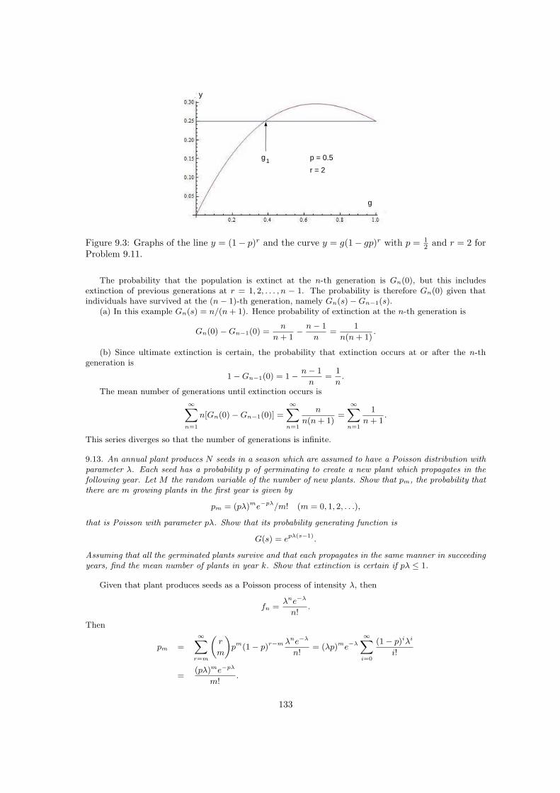
y
g
g1 p = 0.5
r = 2
Figure 9.3: Graphs of the line y = (1− p)r and the curve y = g(1− gp)r with p = 12 and r = 2 for
Problem 9.11.
The probability that the population is extinct at the n-th generation is Gn(0), but this includesextinction of previous generations at r = 1, 2, . . . , n − 1. The probability is therefore Gn(0) given thatindividuals have survived at the (n− 1)-th generation, namely Gn(s)−Gn−1(s).
(a) In this example Gn(s) = n/(n + 1). Hence probability of extinction at the n-th generation is
Gn(0)−Gn−1(0) =n
n + 1− n− 1
n=
1
n(n + 1).
(b) Since ultimate extinction is certain, the probability that extinction occurs at or after the n-thgeneration is
1−Gn−1(0) = 1− n− 1
n=
1
n.
The mean number of generations until extinction occurs is
∞∑n=1
n[Gn(0)−Gn−1(0)] =
∞∑n=1
n
n(n + 1)=
∞∑n=1
1
n + 1.
This series diverges so that the number of generations is infinite.
9.13. An annual plant produces N seeds in a season which are assumed to have a Poisson distribution withparameter λ. Each seed has a probability p of germinating to create a new plant which propagates in thefollowing year. Let M the random variable of the number of new plants. Show that pm, the probability thatthere are m growing plants in the first year is given by
pm = (pλ)me−pλ/m! (m = 0, 1, 2, . . .),
that is Poisson with parameter pλ. Show that its probability generating function is
G(s) = epλ(s−1).
Assuming that all the germinated plants survive and that each propagates in the same manner in succeedingyears, find the mean number of plants in year k. Show that extinction is certain if pλ ≤ 1.
Given that plant produces seeds as a Poisson process of intensity λ, then
fn =λne−λ
n!.
Then
pm =
∞∑r=m
(r
m
)pm(1− p)r−m λne−λ
n!= (λp)me−λ
∞∑i=0
(1− p)iλi
i!
=(pλ)me−pλ
m!.
133
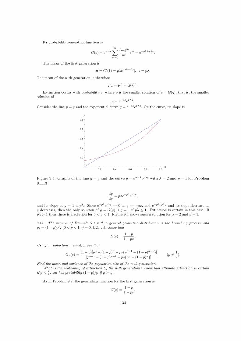
Its probability generating function is
G(s) = e−pλ
∞∑m=0
(pλ)m
m!sm = e−pλ+pλs.
The mean of the first generation is
µ = G′(1) = pλepλ(s−1)|s=1 = pλ.
The mean of the n-th generation is therefore
µn = µn = (pλ)n.
Extinction occurs with probability g, where g is the smaller solution of g = G(g), that is, the smallersolution of
g = e−pλepλg.
Consider the line y = g and the exponential curve y = e−pλepλg. On the curve, its slope is
0.2 0.4 0.6 0.8 1.0g
0.2
0.4
0.6
0.8
1.0
y
Figure 9.4: Graphs of the line y = g and the curve y = e−pλepλg with λ = 2 and p = 1 for Problem9.11.3
dy
dg= pλe−pλepλg,
and its slope at g = 1 is pλ. Since e−pλepλg → 0 as g → −∞, and e−pλepλg and its slope decrease asg decreases, then the only solution of g = G(g) is g = 1 if pλ ≤ 1. Extinction is certain in this case. Ifpλ > 1 then there is a solution for 0 < g < 1. Figure 9.4 shows such a solution for λ = 2 and p = 1.
9.14. The version of Example 9.1 with a general geometric distribution is the branching process withpj = (1− p)pj, (0 < p < 1; j = 0, 1, 2, . . .). Show that
G(s) =1− p
1− ps.
Using an induction method, prove that
Gn(s) =(1− p)[pn − (1− p)n − ps{pn−1 − (1− p)n−1}]
[pn+1 − (1− p)n+1 − ps{pn − (1− p)n}] , (p 6= 1
2).
Find the mean and variance of the population size of the n-th generation.What is the probability of extinction by the n-th generation? Show that ultimate extinction is certain
if p < 12, but has probability (1− p)/p if p > 1
2.
As in Problem 9.2, the generating function for the first generation is
G(s) =1− p
1− ps.
134
Consider
Gn(G(s)) =(1− p)[pn − (1− p)n − p[(1− p)/(1− ps)]{pn−1 − (1− p)n−1}]
[pn+1 − (1− p)n+1 − p[(1− p)/(1− ps)]{pn − (1− p)n}]
=(1− p)[{pn − (1− p)n}(1− ps)− p(1− p){pn−1 − (1− p)n−1}]{pn+1 − (1− p)n+1}(1− ps)− p(1− p){pn−1 − (1− p)n−1}
=(1− p)[pn+1 − (1− p)n+1 − ps{pn − (1− p)n}]
pn+2 − (1− p)n+2 − ps{pn+1 − (1− p)n+1}= Gn+1(s).
Hence if the formula is true for Gn(s), then it is true for Gn+1(s). It can be verified for G2(s), so that byinduction on the integers, it is true for all n.
The probability of extinction by the n-th generation is
Gn(0) =(1− p)[pn − (1− p)n]
pn+1 − (1− p)n+1.
If p > 12, express in the following form
Gn(0) =(1− p)[1− ((1− p)/p)n]
p[1− ((1− p)/p)n+1]→ 1− p
p
as n →∞, which is the probability of ultimate extinction. If p < 12, then
Gn(0) =[(p/(1− p))n − 1]
[(p/(1− p))n+1 − 1]→ 1,
as n →∞: extinction is certain.
9.15. A branching process starts with one individual, and the probability of producing j descendants hasthe distribution {pj}, (j = 0, 1, 2, . . .). The same probability distribution applies independently to alldescendants and their descendants. If Xn is the random variable of the size of the n-th generation, showthat
E(Xn) ≥ 1−P(Xn = 0).
In Section 9.3 it was shown that E(Xn) = µn, where µ = E(X1). Deduce that the probability of extinctioneventually is certain if µ < 1.
By definition
E(Xn) =
∞∑j=1
jP(Xn = j) ≥∞∑
j=1
P(Xn = j) = 1−P(Xn = 0).
HenceP(Xn = 0) = 1− µn.
Therefore, if µ < 1, then P(Xn = 0) → 1 as n →∞. This conclusion is true irrespective of the distribution.
9.16. In a branching process starting with one individual, the probability that any individual has j descen-dants is pj = α/2j, (j = 0, 1, 2, . . . , r), where α is a constant and r is fixed. This means that any individualcan have a maximum of r descendants. Find α and the probability generating function G(s) of the firstgeneration. Show that the mean size of the n-th generation is
µn =
[2r+1 − 2− r
2r+1 − 1
]n
.
What is the probability of ultimate extinction?
Given pj = α/2j , then for it to be a probability distribution
r∑j=0
α
2j= α
[1 +
1
2+
1
22+ · · ·+ 1
2r
]= 2α
[1−
(1
2
)r+1]
= 1.
135
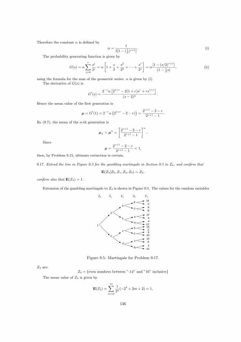
Therefore the constant α is defined by
α =1
2[1− ( 12)r+1]
. (i)
The probability generating function is given by
G(s) = α
r∑j=0
sj
2j= α
[1 +
s
2+
s2
22+ · · ·+ sr
2r
]= α
[1− (s/2)r+1]
(1− 12s)
, (ii)
using the formula for the sum of the geometric series: α is given by (i).The derivative of G(s) is
G′(s) =2−rα
[21+r − 2(1 + r)sr + rs1+r
]
(s− 2)2.
Hence the mean value of the first generation is
µ = G′(1) = 2−rα(21+r − 2− r)
)=
2r+1 − 2− r
2r+1 − 1.
By (9.7), the mean of the n-th generation is
µn = µn =
[2r+1 − 2− r
2r+1 − 1
]n
.
Since
µ =2r+1 − 2− r
2r+1 − 1< 1,
then, by Problem 9.15, ultimate extinction is certain.
9.17. Extend the tree in Figure 9.3 for the gambling martingale in Section 9.5 to Z4, and confirm that
E(Z4|Z0, Z1, Z2, Z3) = Z3.
confirm also that E(Z4) = 1.
Extension of the gambling martingale to Z4 is shown in Figure 9.5. The values for the random variables
1
2
0
4
0
2
-2
8
0
4
-4
6
-2
2
-6
1608
-8
12-44
-1214-26
-1010-6
2-14
0 1Z Z 3Z2Z 4Z
Figure 9.5: Martingale for Problem 9.17.
Z4 are:Z4 = {even numbers between ”-14” and ”16” inclusive}
The mean value of Z4 is given by
E(Z4) =
15∑m=0
1
24(−24 + 2m + 2) = 1,
136
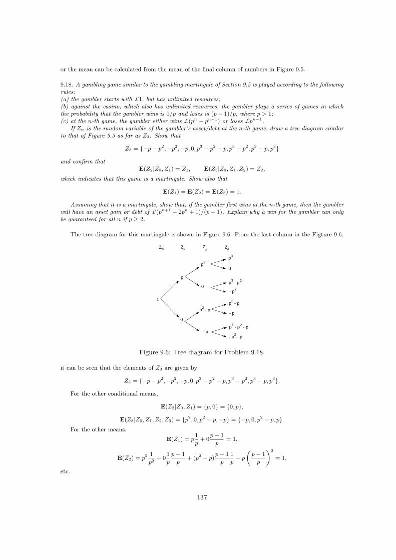
or the mean can be calculated from the mean of the final column of numbers in Figure 9.5.
9.18. A gambling game similar to the gambling martingale of Section 9.5 is played according to the followingrules:(a) the gambler starts with £1, but has unlimited resources;(b) against the casino, which also has unlimited resources, the gambler plays a series of games in whichthe probability that the gambler wins is 1/p and loses is (p− 1)/p, where p > 1;(c) at the n-th game, the gambler either wins £(pn − pn−1) or loses £pn−1.
If Zn is the random variable of the gambler’s asset/debt at the n-th game, draw a tree diagram similarto that of Figure 9.3 as far as Z3. Show that
Z3 = {−p− p2,−p2,−p, 0, p3 − p2 − p, p3 − p2, p3 − p, p3}
and confirm thatE(Z2|Z0, Z1) = Z1, E(Z3|Z0, Z1, Z2) = Z2,
which indicates that this game is a martingale. Show also that
E(Z1) = E(Z2) = E(Z3) = 1.
Assuming that it is a martingale, show that, if the gambler first wins at the n-th game, then the gamblerwill have an asset gain or debt of £(pn+1 − 2pn + 1)/(p− 1). Explain why a win for the gambler can onlybe guaranteed for all n if p ≥ 2.
The tree diagram for this martingale is shown in Figure 9.6. From the last column in the Figture 9.6,
1
0 1Z Z 3Z2
Z
p
p2p3
0
p2 - p
- p
0
p3 - p2
- p2
p3 - p
- p
p3 - p2 - p
p2 - p-
0
Figure 9.6: Tree diagram for Problem 9.18.
it can be seen that the elements of Z3 are given by
Z3 = {−p− p2,−p2,−p, 0, p3 − p2 − p, p3 − p2, p3 − p, p3}.
For the other conditional means,
E(Z2|Z0, Z1) = {p, 0} = {0, p},
E(Z3|Z0, Z1, Z2, Z3) = {p2, 0, p2 − p,−p} = {−p, 0, p2 − p, p}.For the other means,
E(Z1) = p1
p+ 0
p− 1
p= 1,
E(Z2) = p2 1
p2+ 0
1
p
p− 1
p+ (p2 − p)
p− 1
p
1
p− p
(p− 1
p
)2
= 1,
etc.
137
Suppose the gambler first wins at the nth game: on the tree the path will be lowest track until the lastgame. Generalising the path for Z3, the gambler has an asset of
£(pn − 1− p− p2 − · · · − pn−1) = £
[pn −
(pn − 1
p− 1
)]= £
[pn+1 − 2pn + 1
p− 1
].
To guarantee winnings requires
pn+1 − 2pn + 1 = pn(p− 1)+ > 0
for all n. This will certainly be true if p > 2. A smaller value of p will guarantee winnings but this dependson n.
9.19. Let X1, X2, . . . be independent random variables with means µ1, µ2, . . . respectively. Let
Zn = X1 + X2 + · · ·+ Xn,
and let Z0 = X0 = 0. Show that the random variable
Yn = Zn −n∑
i=1
µi, (n = 1, , 2, . . .)
is a martingale with respect to {Xn}. [Note that E(Zn|X1, X2, . . . , Xn) = Zn.]
The result follows since
E(Yn+1|X1, X2, . . . , Xn) = E(Zn+1 −n+1∑i=1
µi|X1, X2, . . . , Xn)
= E(Zn + Xn+1 −n+1∑i=1
µi|X1, X2, . . . , Xn)
= Zn + µn+1 −n+1∑i=1
µi
= Zn −n∑
i=1
µi = Yn
Hence the random variable Yn is a martingale.
9.20. Consider an unsymmetric random walk which starts at the origin. The walk advances one positionwith probability p and retreats one position with probability 1 − p. Let Xn be the random variable givingthe position of the walk at step n. Let Zn be the random variable given by
Zn = Xn + (1− 2p)n.
Show thatE(Z2|X0, X1) = {−2p, 2− 2p} = Z1.
Generally show that {Zn} is a martingale with respect to {Xn}.
The conditional mean
E(Z2|X0, X1) = E(X2 + (1− 2p)2|X0, X1)
= E(X2|X0, X1) + 2(1− 2p)
= {1 + 1− 2p,−1 + 1− 2p} = {2− 2p,−2p} = Z1
By the Markov property of the random walk,
E(Zn+1|X0, X1, . . . , Xn) = E(Zn+1|Xn) = E(Xn+1 + (1− 2p)(n + 1)|Xn)
138
Suppose that Xn = k. Then the walk either advances one step with probability p or retreats one step withprobability 1− p. Therefore
E(Xn+1 + (1− 2p)(n + 1)|Xn) = p(k + 1) + (1− p)(k − 1) + (1− 2p)(n + 1)
= k + (1− 2p)n = Xn.
9.21. In the gambling martingale of Section 9.5, the random variable Zn, the gambler’s asset, in a gameagainst a casino in which the gambler starts with £1 and doubles the bid at each play is given by
Zn = {−2n + 2m + 2}, (m = 0, 1, 2, . . . , 2n − 1).
Find the variance of Zn. What is the variance of
E(Zn|Z0, Z1, . . . , Zn−1)?
Then the sum of the elements in the set Zn = {−2n + 2m + 2}, m = 0, 1, 2, . . . , 2n − 1) is required,that is,
2n−1∑m=0
Zn =
2n−1∑m=0
(−2n + 2m + 2) = (−2n + 2)2n + 2
2n−1∑m=1
m = 2n
Since all the elements in are equally likely to occur after n steps, then
E(Zn) =1
2n
2n−1∑m=0
Zn =1
2n2n = 1.
The variance of Zn is given by
V(Zn) = E(Z2n)− [E(Zn)]2 =
1
2n
2n−1∑m=0
(−2n + 2m + 2)2 − 1 =1
3(22n − 1),
since2n−1∑m=0
(−2n + 2m + 2)2 =2n
3(2 + 22n).
SinceE(Zn|Z0, Z1, . . . , Zn−1) = Zn−1,
then
V[E(Zn|Z0, Z1, . . . , Zn−1)] = V(Zn−1) =1
3[22(n−1) − 1]
by the previous result.
9.22. A random walk starts at the origin, and, with probability p1 advances one position and with probabilityq1 = 1−p1 retreats one position at every step. After 10 steps the probabilities change to p2 and q2 = 1−p2
respectively. What is the expected position of the walk after a total of 20 steps?
After 10 steps the walk could be at any position in the list of even positions
{−10,−8,−6 . . . 6, 8, 10},
which are the random variable Xr. Let the random variable Yn be the position of the walk after 20 stepsso that
Yn = {−20,−18,−16, . . . , 16, 18, 20}.
139
Then the position after a further 10 steps is
E(Yn|Xr) = Xr + 10(p2 − q2).
Its expected position is
E[E(Yn|Xr)] = E[Xr + 10(p2 − q2)] = 10(p1 + p2 − q1 − q2).
9.23. A symmetric random walk starts at the origin x = 0. The stopping rule that the walk ends when theposition x = 1 is first reached is applied, that is the stopping time T is given by
T = min{n : Xn = 1},
where Xn is the position of the walk at step n. What is the expected value of T? If this walk was interpretedas a gambling problem in which the gambler starts with nothing with equal odds of winning or losing £1at each play, what is the flaw in this stopping rule as a strategy of guaranteeing a win for the gambler inevery game? [Hint: the generating function for the probability of the first passage is
G(s) = [1− (1− s2)12 ]/s :
see Problem 3.11.]
The probability generating function for the first passage to x = 1 for the walk starting at the origin is
G(s) =1
s[1− (1− s2)
12 ] =
s
2+
s3
8+
s5
16+ O(s7),
which imples that the probability that the first visit to x = 1 occurs at the 5-th step is 1/16.The mean of the first visits is
µ = G′(s)|s=1 =1− (1− s2)
12
s2(1− s2)12
∣∣∣∣s=1
= ∞.
It seems a good ploy but would take, on average, an infinite number of plays to win £1.
9.24. In a finite-state branching process, the descendant probabilities are, for every individual,
pj =2m−j
2m+1 − 1, (j = 0, 1, 2, . . . , m),
and the process starts with one individual. Find the mean size of the first generation. If Xn is a randomvariable of the size of the n-th generation, explain why
Zn =
[2m+1 − 1
2m+1 −m− 2
]n
Xn
defines a martingale over {Xn}.
In this model of a branching process each descendant can produce not more than m individuals. It canbe checked that
m∑j=0
pj =
m∑j=0
2m−j
2m+1 − 1= 1,
using the formula for the sum of the geometric series.The probability generating function for the first generation is
G(s) =
m∑j=0
pjsj =
2m
2m+1 − 1
m∑j=0
(s
2
)j
=2m+1 − sm+1
(2m+1 − 1)(2− s).
140
Its first derivative is
G′(s) =2m+1 − 2(m + 1)sm + msm+1
(2m+1 − 1) (2− s)2.
Therefore the mean of the first generation is
µ = G′(1) =2m+1 −m− 2
2m+1 − 1.
The random variable Zn is simply Zn = Xn/µn (see Section 9.5).
9.25. A random walk starts at the origin, and at each step the walk advances one position with probabilityp or retreats with probability 1− p. Show that the random variable
Yn = X2n + 2(1− 2p)nXn + [(2p− 1)2 − 1]n + (2p− 1)2n2,
where Xn is the random variable of the position of the walk at time n, defines a martingale with respect to{Xn}.
Let α(p, n) = 2(1− 2p)n and β(p, n) = [(2p− 1)2 − 1]n + (2p− 1)2n2 in the expression for Yn. Then
E(Yn+1|Xn) = p[(Xn + 1)2 + α(p, n + 1)(Xn + 1) + β(p, n + 1)]
+(1− p)[(Xn − 1)2 + α(p, n + 1)(Xn − 1) + β(p, n + 1)]
= X2n + Xn[4p− 2 + α(p, n + 1)] + [1 + (2p− 1)α(p, n + 1) + β(p, n + 1)]
The coefficients in the last expression are
4p− 2 + α(p, n + 1) = 4p− 2 + 2(1− 2p)(n + 1) = 2(1− 2p)n = α(p, n),
and
1 + (2p− 1)α(p, n + 1) + β(p, n + 1) =
1 + (2p− 1)2(1− 2p)(n + 1) + [(2p− 1)2 − 1](n + 1) + (2p− 1)2(n + 1)2
= [(2p− 1)2 − 1]n + (2p− 1)2n2 = β(p, n)
HenceE(Yn+1|Xn) = X2
n + 2(1− 2p)nXn + [(2p− 1)2 − 1]n + (2p− 1)2n2 = Yn,
so that, by definition, Yn is a martingale.
9.26. A simple epidemic has n0 susceptibles and one infective at time t = 0. If pn(t) is the probability thatthere are n susceptibles at time t, it was shown in Section 9.7 that pn(t) satisfies the differential-differenceequations (see eqns (9.15 and (9.16))
dpn(t)
dt= β(n + 1)(n0 − n)pn+1(t)− βn(n0 + 1− n)pn(t),
for n = 0, 1, 2, . . . n0. Show that the probability generating function
G(s, t) =
n0∑n=0
pn(t)sn
satisfies the partial differential equation
∂G(s, t)
∂t= β(1− s)
[n0
∂G(s, t)
∂s− s
∂2G(s, t)
∂s2
].
Nondimensionalize the equation by putting τ = βt. For small τ let
G(s, τ/β) = G0(s) + G1(s)τ + G2(s)τ2 + · · · .
141
Show that
nGn(s) = n0(1− s)∂Gn−1(s)
∂s− s(1− s)
∂2Gn−1(s)
∂s2,
for n = 1, 2, 3, . . . n0. What is G0(s)? Find the coefficients G1(s) and G2(s). Hence show that the meannumber of infectives for small τ is given by
n0 − n0τ − 1
2n0(n0 − 2)τ2 + O(τ3).
In Example 9.9, the number of susceptibles initially is given by n0 = 4. Expand p0(t), p1(t) and p2(t)in powers of τ and confirm that the expansions agree with G1(s) and G2(s) above.
Multiply the difference equation by s and sum from s = 0 to s = n0 giving
n0∑n=0
p′(t)sn = β
n0−1∑n=0
(n + 1)(n0 − n)pn+1(t)− β
n0∑n=1
n(n0 + 1− n)pn(t)sn,
or,
Gt(s, t) = βn0
n0∑m=1
mpm(t)sm−1 − β
n0∑m=2
m(m− 1)pm(t)sm−1 − βn0
n0∑n=1
npn(t)sn
+β
n0∑n=1
n(n− 1)pn(t)sn
= βn0Gs(s, t)− βsGss(s, t)− βn0sGs(s, t) + βs2Gss(s, t)
= βn0(1− s)Gs(s, t) + βs(s− 1)Gss(s, t),
as required.Let τ = βt. Then the equation for H(s, τ) = G(s, τ/β) is
∂H(s, τ)
∂τ= (1− s)
[n0
∂H(s, τ)
∂s− s
∂2H(s, τ)
∂s2
].
For small τ , letH(s, τ) = G(s, τ/β) = H0(s) + H1(s)τ + H2(s)τ
2 + · · · ,and substitute this series into the partial differential equation for H(s, τ), so that
H1(s) + 2H2(s)τ + · · · = (1− s)n0[H′0(s) + H ′
1(s)τ + · · ·]− s(1− s)n0[H′′0 (s) + H ′′
1 (s)τ + · · ·].
Equating powers of τ , we obtain
nHn(s) = (1− s)n0H′n−1(s)− s(1− s)n0H
′n−1(s), (n = 1, 2, 3, . . .). (i)
For τ = 0,
H0(s) = G(s, 0) =
n0∑n=0
pn(0)sn.
Since the number of susceptibles is n0 at time t = 0. Therefore
pn0(0) = n0, pn(0) = 0, (n 6= n0).
Hence H0(s) = sn0 .From (i),
H1(s) = n0(1− s)∂H0(s)
∂s− s(1− s)
∂2H0(s)
∂s2
= n20(1− s)sn0−1 − s(1− s)n0(n0 − 1)sn0−2
= n0(1− s)sn0−1,
142
H2(s) =1
2
[n0(1− s)
∂H1(s)
∂s− s(1− s)
∂2H1(s)
∂s2
]
=1
2n0(1− s)[n0{(n0 − 1)sn0−2 − n0s
n0−1}
−1
2s(1− s)[n0{(n0 − 1)(n0 − 2)sn0−3 − n0(n0 − 1)sn0−2}]
=1
2n0s
n0−2(1− s)(2n0 − 2− n0s)
The mean number of infectives is given by
µ = Hs(1, τ) = H ′0(1) + H ′
1(1)τ + H ′2(1)τ2 + O(τ3)
= n0sn0−1 + [n0(n) − 1)sn0−2 − n2
0sn0−1]τ
+1
2[n3
0sn0−1 + (n0 − 1)(2n0 − 3n2
0)sn0−2 + (n0 − 2)(2n2
0 − 2n0)sn0−3]τ2 + O(τ3)
∣∣∣s=1
= n0 − n0τ − 1
2n0(n0 − 2)τ2 + O(τ3),
where τ = βt.
143