STOCHASTIC WATER QUALITY ANALYSIS USING RELIABILITY METHOD

JOURNAL OF THE AMERICAN WATER RESOURCES ASSOCIATIONVOL. 37, NO. 3 AMERICAN WATER RESOURCES ASSOCIATION JUNE 2001

STOCHASTIC WATER QUALITY ANALYSISUSING RELIABILITY METHOD'

Kun-Yeun Han, Sang-Ho Kim, and Deg-Hyo Bae2

ABSTRACT: This study developed a QUAL2E-Reliability Analysis(QUAL2E-RA) model for the stochastic water quality analysis ofthe downstream reach of the main Han River in Korea. The pro-posed model is based on the QUAL2E model and incorporates theAdvanced First-Order Second-Moment (AFOSM) and Mean-ValueFirst-Order Second-Moment (MFOSM) methods. After thehydraulic characteristics from standard step method are identified,the optimal reaction coefficients are then estimated using theBroyden-Fletcher-Goldfarb-Shanno (BFGS) method. Consideringvariations in river discharges, pollutant loads from tributaries, andreaction coefficients, the violation probabilities of existing waterquality standards at several locations in the river were computedfrom the AFOSM and MFOSM methods, and the results were com-pared with those from the Monte Carlo method. The statistics ofthe three uncertainty analysis methods show that the outputs fromthe AFOSM and MFOSM methods are similar to those from theMonte Carlo method. From a practical model selection perspective,the MFOSM method is more attractive in terms of its computation-al simplicity and execution time.(KEY TERMS: river water quality; stochastic analysis; reliability.)

INTRODUCTION

The current industrial development and populationgrowth in Korea have produced a rapid increase inwastewater discharge. In particular, the aggravationof water quality at locations where intake plants andcontaminated inflow sources coexist causes seriouswater quality problems during low flow periods. Atypical example of such an area is the downstreamreach of the main Han River, which passes throughthe Seoul metropolitan area that has a population of10 million. There are two main reasons that make thewater quality modeling in this area difficult. The first

is related to the different hydraulic characteristicsbetween the upstream and downstream regions due tothe existence of a hydraulic weir in the middle of thereach. The second is the temporal and spatial varia-tion of the water quality that is partially caused byintermittent contaminant inflows from tributariesand partially by seasonal variations in the river flow.

Many stream water quality models have beendeveloped for forecasting and predicting environmen-tal phenomena. However, most of these models havebeen designed to simulate BOD, DO, T-N, and T-P lev-els as deterministic values without considering anyvariability in the model parameters. Since these mod-els are simplified descriptions of the real water quali-ty phenomena, the disregard of model parameteruncertainty can potentially lead to erroneous manage-ment decisions. For example, a slight variation in thedeoxygenation rate constant can result in a huge dif-ference in the cost of a water quality abatementeffort. In this sense, the consideration of modelparameter uncertainty, as well as its average value, isan important issue in water quality modeling study.

Uncertainty analyses in water quality modelingmainly focus on model parameter variability (Schnoor,1996). Among the various methods the Monte Carlosimulation and FORA (first order reliability analysis)techniques are traditionally used. Kothandaramanand Ewing (1969), Warwick and Cale (1987), andQaisi (1988) applied the Monte Carlo method to theStreeter-Phelps equation (1925) and quantified themodel output uncertainties. The QUAL2E-UNCASmodel developed by the US Environmental ProtectionAgency (Brown and Barnwell, 1987) also allows the

iPaper No. 99107 of the Journal of the American Water Resources Association. Discussions are open until February 1, 2002.2Respectively, Professor, Department of Civil Engineering, Kyungpook National University; 1370 Sankyuk-Dong, Puk-Ku, Daegu 702-701,

Korea; Senior Researcher, Water Resources and Environmental Research Division, Korea Institute of Construction Thchnology, 2311 Taehwa-Dang, Ilsan-ku, Koyang, Kyonggi-Do 411-712, Korea; and Associate Professor, Department of Civil Engineering, Changwon National Univer-sity, 9 Sarim-Dong, Changwon City, Kyongsangnam-Do, 641-241, Korea (E-Mail/Han: [email protected]).

JOURNAL OF THE AMERICAN WATER RESOURCES ASSOCIATION 695 JAWRA

Han, Kim, and Bae

modeler to analyze model uncertainty based on theMonte Carlo method. Burges and Lettenmaier (1975),Chadderton et al. (1982), Tung and Hathhorn (1988),and Meiching and Anmangandla (1992) applied theFORA method to the Streeter-Phelps equation andestimated uncertainties using a statistical analysis.Schnoor (1996) and Chapra (1997) presented adetailed procedure for the Monte Carlo and FORAmethods. Warwick (1997) developed a first-orderuncertainty technique to quantify the relationshipbetween field data collection and a modeling exerciseinvolving both calibration and verification. Kuo et al.(1997) applied a two-dimensional water quality modeland incorporated the mean first-order second momentmethod and Monte Carlo method for a risk analysis ofthe Keelung River. More recently, Vasquez et al.(2000) presented an efficient approach for obtainingwasteload allocation solution, which links a geneticalgorithm with the first-order reliability method.

The main objective of this study is to develop awater quality management model for the downstreamreach of the Han River. Due to the complicated flowcharacteristics and varying contaminant inflows inthis region, this study attempts to build a stochasticwater quality model that can facilitate an i.mcertaintyanalysis and consider the variability of the modelparameters. The previous QUAL2E-UNCAS modelwas based on the Monte Carlo method. However, theMonte Carlo method has a serious disadvantage inthat it requires a large number of iterative solutions.Thus, the proposed model, called QUAL2E-RA(QUAL2E-Reliability Analysis), was built based onthe AFOSM (Advanced First-Order Second-Moment)and MFOSM (Mean-Value First-Order Second-Moment) methods, which are relatively simple com-pared to the Monte Carlo method.

The next section presents the basic concept of relia-bility and the proposed model structure based on theAFOSM and MFOSM methods. This is followed by adescription of the study area, and a presentation ofthe results of a deterministic model for quantifyingthe optimal reaction coefficients. Then, the results ofthe stochastic water quality analysis are presented,along with some discussion and conclusions.

Reliability

RELIABILITY ANALYSIS

concentrations (load) should meet the water qualitystandards (resistance) set by the regulatory agency.Risk, which is the complement of reliability, is definedas the probability of failure.

Risk=Pf=P(R<L)=P(R-L<0)=P(Z< 0) (1)

where Pf is the probability of failure; R is the resis-tance; L is the load; P(x) is the probability of event x;and Z is the performance variable. Equation (1)demonstrates that failure occurs if the load is greaterthan the resistance. This is true for most water quali-ty variables except DO. In the case of DO, failureoccurs if the DO concentration is less than the stan-dard (Vasquez et al., 2000). Therefore, the sign ofinequality for DO should be changed in the oppositedirection.

AFOSM Method

The basic concept of the AFOSM method is toreduce the error in the first-order approximation dueto nonlinearity by expanding the Taylor series at afailure point, x = (xi*, x2", x3*, ..., xn*) on the failuresurface. At the failure point x1, the load L is same asthe resistance R and the performance variable Z iszero (Ang and Tang, 1984; Yen et al., 1986).

Several recursive techniques for determining thefailure point have been suggested, among whichRackwitz's method is the best known (Rackwitz, 1976;Rackwitz and Fiessler, 1977; Ang and Tang, 1984). Afirst order approximation of a Taylor series expansionof the performance function Z for unrelated variablesX1 at a failure point can be represented as:

** * * *

Z=g(x1,x2,x3,...,x)+(X1—x•)--——i=1

'ax,

(2)

At the failure surface g(x1*, x2, x3", ..., xn*) = 0, theexpected value and standard deviation of Z are:

E[Z] = -4)

= aiCo1

(3)

(4)

whereReliability is defined as the probabilistic measureof whether a system meets certain standards, and canbe described as a problem of load and resistance. Ina water quality problem, the simulated constituent

JAWRA 696 JOURNAL OF THE AMERICAN WATER RESOURCES ASSOCIATION

C•---1—

ax1(5)

Stochastic Water Quality Analysis Using Reliability Method

The g(xi*) in Equation (2) is a functional represen-tation of the performance variable Z. If all the basicvariables are normally distributed, the risk Pf can berepresented by the following equation.

Pf= 1 -

where, li denotes the reliability index using theAFOSM method, i.e.,

't(131) is the cumulative distribution function (CDF) ofa standard Gaussian distribution for In this study,the aforementioned Rackwitz algorithm is used toidentify x and .

In reality, the basic variables are not usually nor-mally distributed but are skewed with their respec-tive probability distribution, and only the mean andstandard deviation are available. Therefore, the basicnon-normally distributed variables need to be firsttransformed into an equivalent normal distribution,then the AFOSM method can be applied to identifythe reliability index (Rackwitz and Fiessler, 1977;Ang and Tang, 1984; Yen et al., 1986). The proposedmodel is organized to handle normal, log-normal, uni-form, and triangular distributions of water qualitydata.

MFOSM Method

The MFOSM method is based on a Taylor seriesexpansion which is expanded with respect to themean of the variables, 5 =(, x2, x3, ... ,). The first-order approximation of a Taylor series expansion atfor unrelated variables X1 is

—')_

The expected value and standard deviation of Z inthis method can be represented as:

E[Z] =

1/2(6)

rn -1

=Li=i

(10)

As discussed by Yen et al. (1986), the main advan-tages of this approach are that only the mean andvariance of the input parameters are required andthat the uncertainties for the output variables arerepresented by a relatively simple and definite math-ematical expression. If 2 denotes the reliability index

() according to the MFOSM method, the risk Pf can berepresented by the following equation.

Pf = 1 - I32) (11)

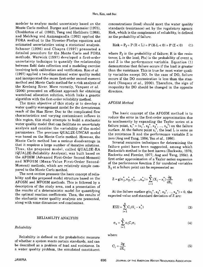
The basic difference between the MFOSM andAFOSM methods is that the former is based on a Tay-lor series expansion at the mean of the variables 5,whereas the latter is based on a Taylor series expan-sion at the failure point xj*. Figure 1 shows a compari-son of the reliability indexes produced by the AFOSMand MFOSM methods.

IMPLEMENTATION OF AFOSM,MFOSM TO QUAL2EU

The enhanced stream water quality modelQUAL2E, which is applicable to dendritic streams, iswidely used for wasteload allocations, water qualityplanning activities, and other conventional pollutantevaluations. The model, which can be operated aseither a steady-state or a quasi-dynamic model, simu-lates the major reactions of nutrient cycles, algal pro-duction, benthic and carbonaceous demand,atmospheric reaeration, and their effects on the dis-solved oxygen balance. The model can predict up to 15water quality constituent concentrations. The deter-ministic water quality analysis model QUAL2E hasone main program and 51 subroutines.

In order to perform the uncertainty analysis of theQUAL2E, the proposed model has three additionalcomponents: a sensitivity analysis, first-order erroranalysis, and Monte Carlo simulation. The sensitivityanalysis computes the variation of the predictions

(8)when one or more parameters and variables arechanged. The first-order error analysis estimates anormalized sensitivity coefficient that represents thepercentage change in the output variable resultingfrom a one percent change in each input variable. TheMonte Carlo simulation works for a complex systemthat has random components. The first-order error

(9) propagation provides a direct estimate of the mo4el


Failure

Figure 1. Comparison of 3 Values Using AFOSM and MFOSM Methods.

sensitivity. The Monte Carlo simulation has anadvantage of acquiring output frequency distribu-tions. However, it requires an extensive computationeffort. Accordingly, the prescribed AFOSM andMFOSM methods are incorporated into the QUAL2E-UNCAS model particularly in relation to the reliabili-ty and uncertainty analyses of the water qualitysimulations.

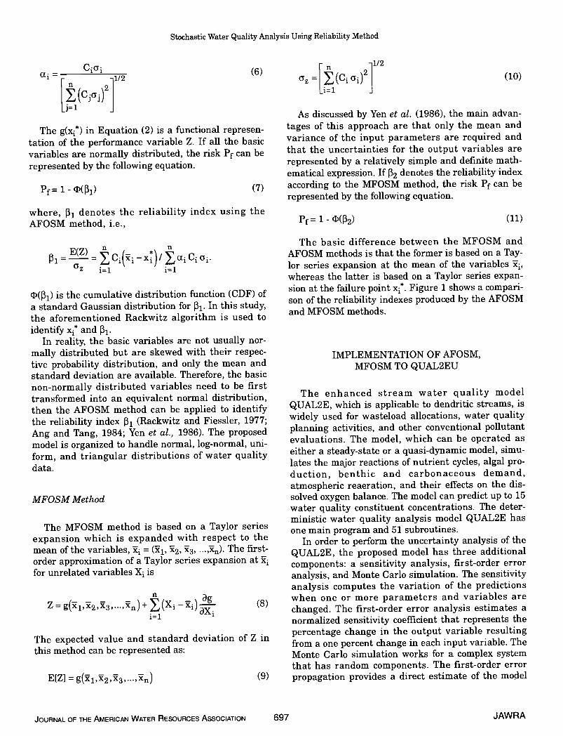
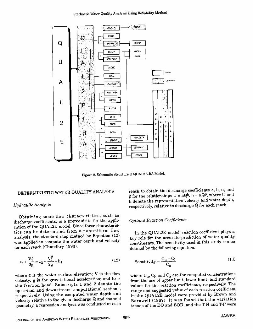
Figure 2 shows the model structure for QUAL2E-RA, where the seven existing subroutines are modi-fied and seven new subroutines are added. SubroutineAFOSM performs uncertainty computations andwrites the report for the AFOSM option, whereas sub-routine MFOSM performs the computations andwrites the report for the MFOSM option. SETUPAFOsets up the input conditions for the AFOSM andMFOSM simulations. REPLBETA restores the per-turbed value to its base case value after the AFOSMsimulation. PROBIL obtains the risk from the relia-bility index. SWAPAFO swaps the perturbed value ofthe input variable for the base case value in theAFOSM option. RSTORAFO restores the base casevalue to the values of the perturbed input data afterthe model runs. Descriptions for the other subrou-tines in Figure 2 are given by Brown and Barnwell(1987).

STUDY AREA

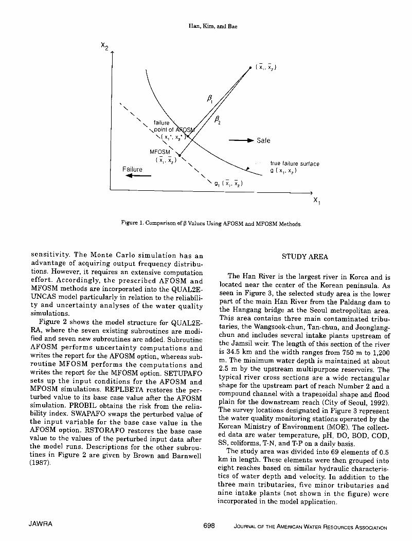
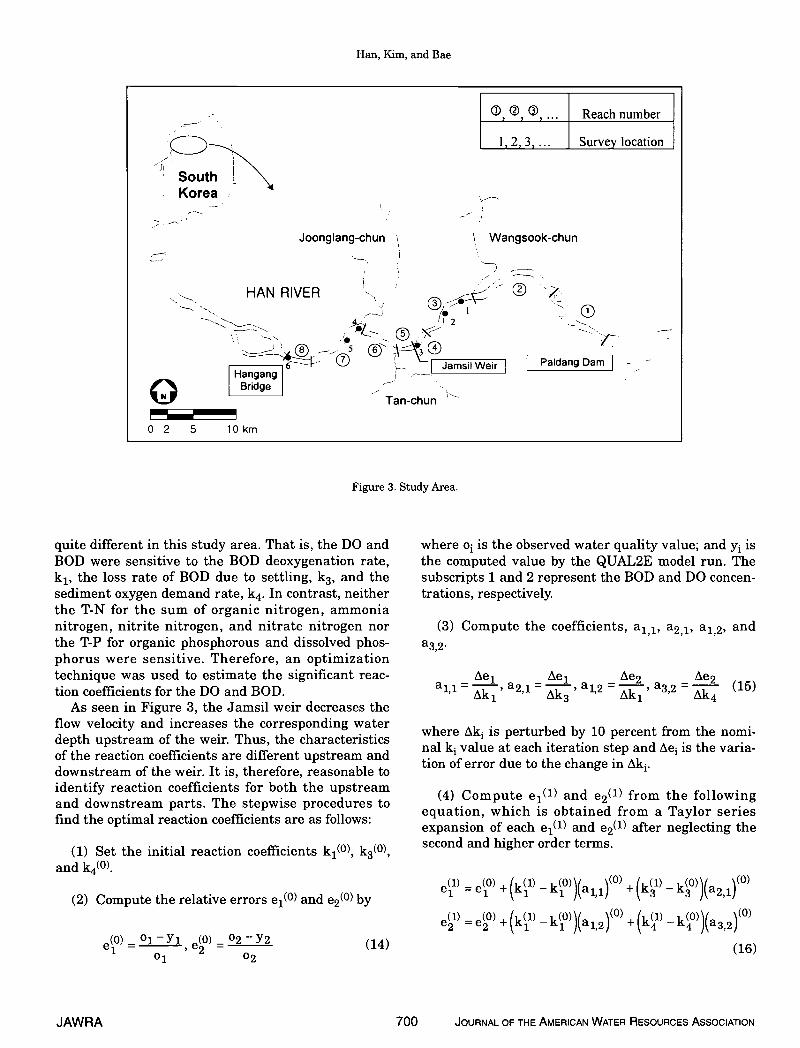
The Han River is the largest river in Korea and islocated near the center of the Korean peninsula. Asseen in Figure 3, the selected study area is the lowerpart of the main Han River from the Paldang dam tothe Hangang bridge at the Seoul metropolitan area.This area contains three main contaminated tribu-taries, the Wangsook-chun, Tan-chun, and Joonglang-chun and includes several intake plants upstream ofthe Jamsil weir. The length of this section of the riveris 34.5 km and the width ranges from 750 m to 1,200m. The minimum water depth is maintained at about2.5 m by the upstream multipurpose reservoirs. Thetypical river cross sections are a wide rectangularshape for the upstream part of reach Number 2 and acompound channel with a trapezoidal shape and floodplain for the downstream reach (City of Seoul, 1992).The survey locations designated in Figure 3 representthe water quality monitoring stations operated by theKorean Ministry of Environment (MOE). The collect-ed data are water temperature, pH, DO, BOD, COD,SS, coliforms, T-N, and T-P on a daily basis.

The study area was divided into 69 elements of 0.5km in length. These elements were then grouped intoeight reaches based on similar hydraulic characteris-tics of water depth and velocity. In addition to thethree main tributaries, five minor tributaries andnine intake plants (not shown in the figure) wereincorporated in the model application.


x2

Han, Kim, and Bae

( x, x2)

N/9'

MFOSMN

- Safe

NN

N g1 (x1,2)

- true failure surfaceQ (xi, x2)

xl


Figure 2. Schematic Structure of QUAL2E-RA Model.

DETERMINISTIC WATER QUALITY ANALYSIS

Hydraulic Analysis

Obtaining some flow characteristics, such asdischarge coefficients, is a prerequisite for the appli-cation of the QUAL2E model. Since these characteris-tics can be determined from a nonuniform flowanalysis, the standard step method by Equation (12)was applied to compute the water depth and velocityfor each reach (Chaudhry, 1993).

vj2z1+—=z2+ +hf2g 2g

(12)

where z is the water surface elevation; V is the flowvelocity; g is the gravitational acceleration; and hf isthe friction head. Subscripts 1 and 2 denote theupstream and downstream computational sections,respectively. Using the computed water depth andvelocity relative to the given discharge Q andchannelgeometry, a regression analysis was conducted at each

reach to obtain the discharge coefficients a, b, a, and3 for the relationships U = aQb, h = aQI, where U andh denote the representative velocity and water depth,respectively, relative to discharge Q for each reach.

Optimal Reaction Coefficients

In the QUAL2E model, reaction coefficient plays akey role for the accurate prediction of water qualityconstituents. The sensitivity used in this study can bedefined by the following equation.

Cu - ClSensitivity =Ca

(13)

where C, C1, and Ca are the computed concentrationsfrom the use of upper limit, lower limit, and standardvalues for the reaction coefficients, respectively. Therange and suggested value of each reaction coefficientin the QUAL2E model were provided by Brown andBarnwell (1987). It was found that the variationtrends of the DO and BOD, and the T-N and T-P were


Han, Kim, and Bae

, , ®, ... Reach number

1, 2, 3, ... Survey location

quite different in this study area. That is, the DO andBOD were sensitive to the BOD deoxygenation rate,k1, the loss rate of BOD due to settling, k3, and thesediment oxygen demand rate, k4. In contrast, neitherthe T-N for the sum of organic nitrogen, ammonianitrogen, nitrite nitrogen, and nitrate nitrogen northe T-P for organic phosphorous and dissolved phos-phorus were sensitive. Therefore, an optimizationtechnique was used to estimate the significant reac-tion coefficients for the DO and BOD.

As seen in Figure 3, the Jamsil weir decreases theflow velocity and increases the corresponding waterdepth upstream of the weir. Thus, the characteristicsof the reaction coefficients are different upstream anddownstream of the weir. It is, therefore, reasonable toidentify reaction coefficients for both the upstreamand downstream parts. The stepwise procedures tofind the optimal reaction coefficients are as follows:

(1) Set the initial reaction coefficients k1(°), k3(°),and k4(°).

(2) Compute the relative errors e1(0) and e2(0) by

= o1—y1 e° = 02y2 (14)01 02

where o is the observed water quality value; and y1 isthe computed value by the QUAL2E model run. Thesubscripts 1 and 2 represent the BOD and DO concen-trations, respectively.

(3) Compute the coefficients, a11, a2,1, a1,2, anda3,2.

ai,1=———,a2,1=-———,a1,2=———,a3,2=------- (15)

where i\k is perturbed by 10 percent from the nomi-nal k1 value at each iteration step and i\e is the varia-tion of error due to the change in i\k.

(4) Compute e11 and e2(') from the followingequation, which is obtained from a Taylor seriesexpansion of each e11 and e2(1) after neglecting thesecond and higher order terms.

= +(k1)

— k)(ai,i)° + (ks') — k°))(a2,i)°

e =e° +(kçl)

—

k°))(ai,2)° +(k —

k")(a3,2)°(16)


SouthKorea

Joonglang-chun Wangsook-chun

HANRIVER ® ?r2

5 ____ _____Jamsil Weir I Paldang Dam

HangangBridge

N Tan-chun

0 2 5 10km

Figure 3. Study Area.


where the reaction coefficients k1('), k3'), and k4(1)are obtained by the BFGS (Broyden-Fletcher-Gold-farb-Shanno) optimization technique (Vanderplaats,1984).

(5) Optimize k1, k3, and k4 by minimizing the sumof the squared error S under the given constraints as:

Mm s ={(e1))2 +(41))2}

subject to

k31 �k3

k41�k4

where the superscripts u and 1 represent the upperand lower limits for the variable.

(6) Stop the iteration if the value of the minimizedsquared error S is within the stopping criteria. Other-wise, a new iteration with k1'), k3('), and k4(') as theinitial conditions is performed through Steps 1 to 5.

The BFGS technique is an improved optimizationmethod developed from the variable metric methodcalled the quasi-Newton method. As seen in Equation(18), this method obtains an approximate solutionusing a first-order derivative instead of computing theinverse of a Hessian matrix.

G'1 =Gi _[GAgAnT +AnAgTG]'[

[11+AgTGAg' AnAnT 1

LL AnTAg ) AnTAg](18)

17where i is the iteration number; n is the parametervector; g is the gradient vector; and A is the differencebetween the two iterations (Ag gi - gil). It is gener-ally known that, among the various optimization algo-rithms, the BFGS technique produces the best globaloptimal solution from numerical experiments (Dennisand More, 1977).

Model Calibration and Verification

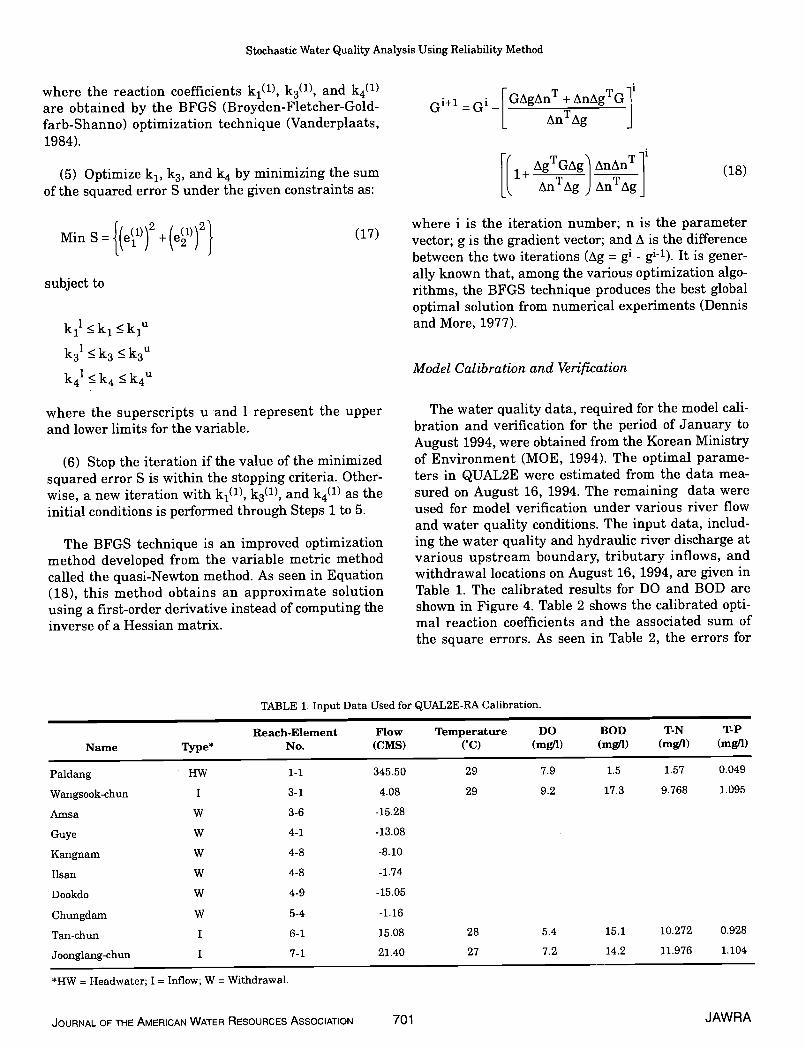
The water quality data, required for the model cali-bration and verification for the period of January toAugust 1994, were obtained from the Korean Ministryof Environment (MOE, 1994). The optimal parame-ters in QUAL2E were estimated from the data mea-sured on August 16, 1994. The remaining data wereused for model verification under various river flowand water quality conditions. The input data, includ-ing the water quality and hydraulic river discharge atvarious upstream boundary, tributary inflows, andwithdrawal locations on August 16, 1994, are given inTable 1. The calibrated results for DO and BOD areshown in Figure 4. Table 2 shows the calibrated opti-mal reaction coefficients and the associated sum ofthe square errors. As seen in Table 2, the errors for

TABLE 1. Input Data Used for QUAL2E-RA Calibration.

Name Type*Reach-Element

No.Flow(CMS)

TemperatureCC)

DO(mg/I)

BOD(mg/i)

T-N(mg/i)

T-P(mg/I)

Paldang• MW 1-1 345.50 29 7.9 1.5 1.57 0.049

Wangsook-chun I 3-1 4.08 29 9.2 17.3 9.768 1.095

Amsa W 3-6 -15.28

Guye W 4-1 -13.08

Kangnam W 4-8 -8.10

Ilsan W 4-8 -1.74

Dookdo W 4-9 -15.05

Chungdam W 5-4 -1.16

Tan-chun I 6-1 15.08 28 5.4 15.1 10.272 0.928

Joonglang-chun I 7-1 21.40 27 7.2 14.2 11.976 1.104

*IW = Headwater; I = Inflow; W = Withdrawal.


Han, Kim, and Bae

10.0

0.0 L

Distance ( km)

Figure 4. Results of Model Calibration Using the Data on August 16, 1994.

upstream and downstream of the Jamsil weir were0.082 and 0.116, respectively, and the iterations wereconverged within two steps. It was also obtained thatthe correlation coefficients between the observed andthe computed DO and BOD values during the modelcalibration period were 0.995 and 0.967, respectively.Accordingly, the calibrated results were in good agree-ment with the observed ones.

Iteration k1 k3 S

Upstream of Jamsil Weir

0

1

2

0.261 0.0 0.9840.239 0.0 3.8820.258 0.0 3.691

0.1680.0840.082

Downstream of Jamsil Weir

0

1

2

0.261 0.00 0.9840.350 -0.18 3.0020.335 -0.17 2.958

0.1680.1200.116

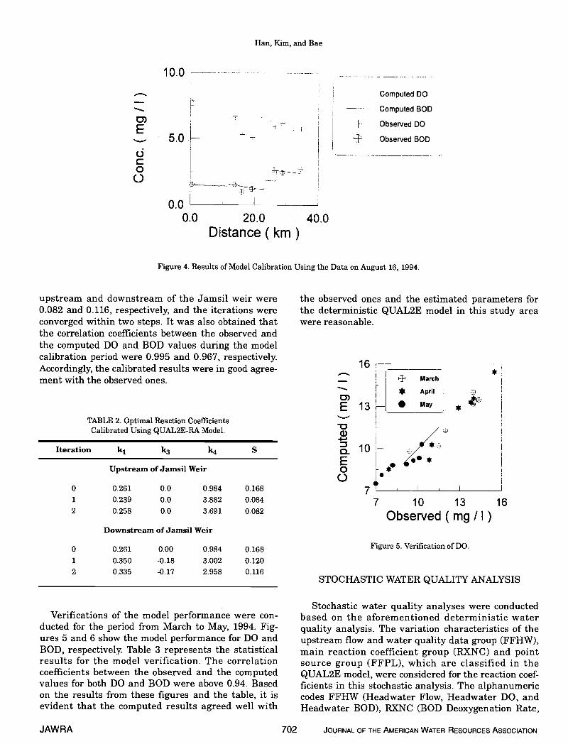
Verifications of the model performance were con-ducted for the period from March to May, 1994. Fig-ures 5 and 6 show the model performance for DO andBOD, respectively. Table 3 represents the statisticalresults for the model verification. The correlationcoefficients between the observed and the computedvalues for both DO and BOD were above 0.94. Basedon the results from these figures and the table, it isevident that the computed results agreed well with

the observed ones and the estimated parameters forthe deterministic QUAL2E model in this study areawere reasonable.

* Aprilf! 13H_I May *

//In1.)

*

7-.

7 10 13 16

Observed (mg/I)

STOCHASTIC WATER QUALITY ANALYSIS

Stochastic water quality analyses were conductedbased on the aforementioned deterministic waterquality analysis. The variation characteristics of theupstream flow and water quality data group (FFHW),main reaction coefficient group (RXNC) and pointsource group (FFPL), which are classified in theQUAL2E model, were considered for the reaction coef-ficients in this stochastic analysis. The alphanumericcodes FFHW (Headwater Flow, Headwater DO, andHeadwater BOD), RXNC (BOD Deoxygenation Rate,


0)E

000

-I- +

H-F

±±

Computed DO

Computed BOD

-f- Observed DO

P Observed BOD

0.0 20.0 40.0

16

TABLE 2. Optimal Reaction CoefficientsCalibrated Using QUAL2E-RA Model. a)

0E00

Figure 5. Verification of DO.


Loss Rate of BOD due to Settling, and Sediment Oxy-gen Demand Rate), and FFPL (Point Load Flow, PointLoad DO, and Point Load BOD) represent the namesof the generic groups of input variables to be variedfor the uncertainty analysis. The selected range ofinput variation was based on a statistical analysis ofthe observed data over the previous 10 years for theHan River (MOE, 1985-1994).

March April May

DO 0.998 0.997 0.996

BOD 0.976 0.946 0.974

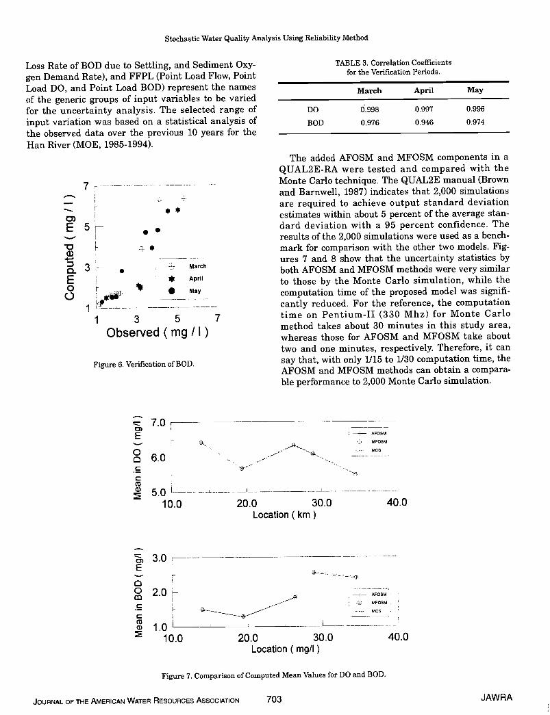
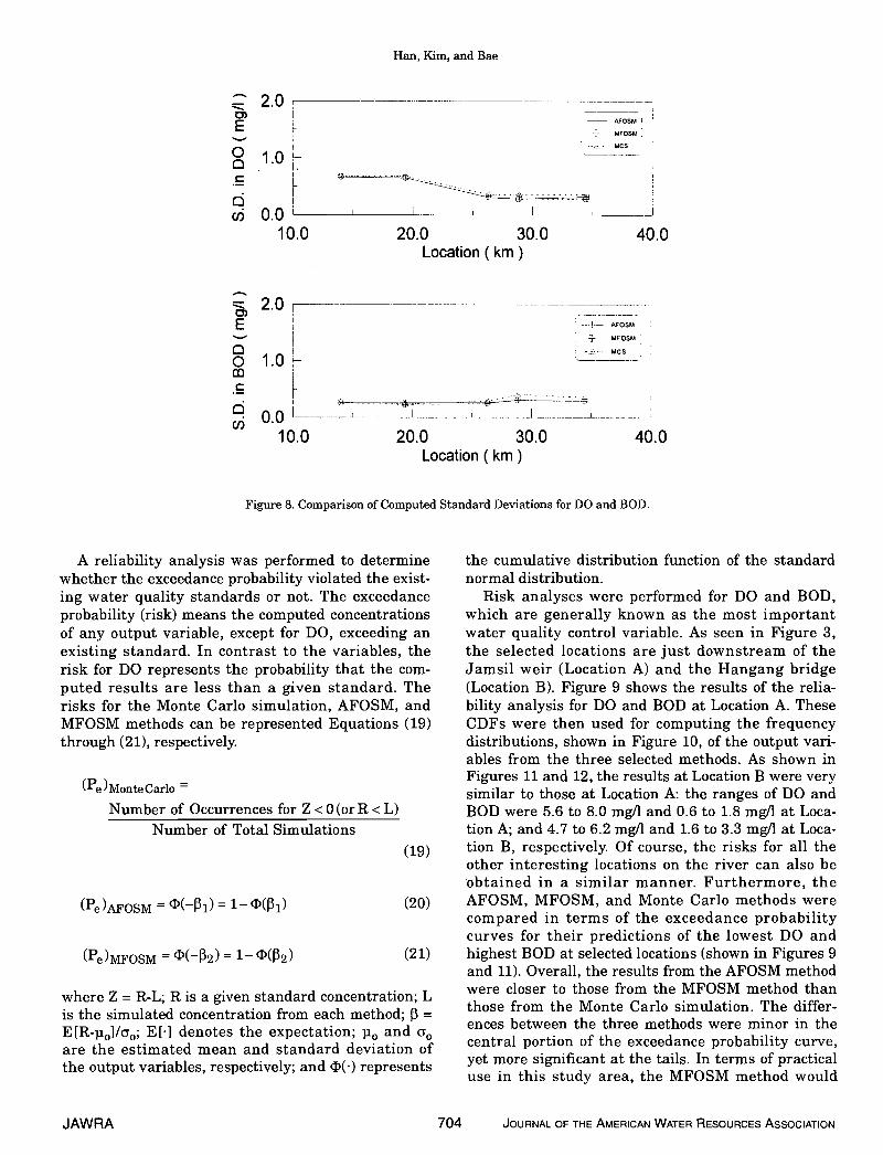
The added AFOSM and MFOSM components in aQUAL2E-RA were tested and compared with theMonte Carlo technique. The QUAL2E manual (Brownand Barnwell, 1987) indicates that 2,000 simulationsare required to achieve output standard deviationestimates within about 5 percent of the average stan-dard deviation with a 95 percent confidence. Theresults of the 2,000 simulations were used as a bench-mark for comparison with the other two models. Fig-ures 7 and 8 show that the uncertainty statistics byboth AFOSM and MFOSM methods were very similarto those by the Monte Carlo simulation, while thecomputation time of the proposed model was signifi-cantly reduced. For the reference, the computationtime on Pentium-Il (330 Mhz) for Monte Carlomethod takes about 30 minutes in this study area,whereas those for AFOSM and MFOSM take abouttwo and one minutes, respectively. Therefore, it cansay that, with only 1115 to 1/30 computation time, theAFOSM and MFOSM methods can obtain a compara-ble performance to 2,000 Monte Carlo simulation.

.—-

Location (km)

—f— AFOSM

-' MFOSMMCS

30.0 40.0Location (mg/I)

Figure 7. Comparison of Computed Mean Values for DO and BOD.


TABLE 3. Correlation Coefficientsfor the Verification Periods.

C)E

a)

E00

7

5-3— March

* AprIl

•MayI

1 3 5 7

Observed(mg/I)

Figure 6. Verification of BOD.

7.0 —C)E

o 6.0 H-CC

5.0 c—--10.0

C)E

2.0H

10.0

—4— AFOSM

+MCS

40.020.0 30.0

—

20.0

Han, Kim, and Bae

Figure 8. Comparison of Computed Standard Deviations for DO and BOD.

A reliability analysis was performed to determinewhether the exceedance probability violated the exist-ing water quality standards or not. The exceedanceprobability (risk) means the computed concentrationsof any output variable, except for DO, exceeding anexisting standard. In contrast to the variables, therisk for DO represents the probability that the com-puted results are less than a given standard. Therisks for the Monte Carlo simulation, AFOSM, andMFOSM methods can be represented Equations (19)through (21), respectively.

We )Monte Carlo =

Number of Occurrences for Z <0(or R < L)Number of Total Simulations

(1e)jU'OSM I(—I3i) = 1— Ui)

(Pe)MFOSM = L(—32) = 1— I(f32)

where Z = R-L; R is a given standard concentration; Lis the simulated concentration from each method; 3 =E[R-J101/G0; EEl denotes the expectation; lo and oare the estimated mean and standard deviation ofthe output variables, respectively; and '1*) represents

the cumulative distribution function of the standardnormal distribution.

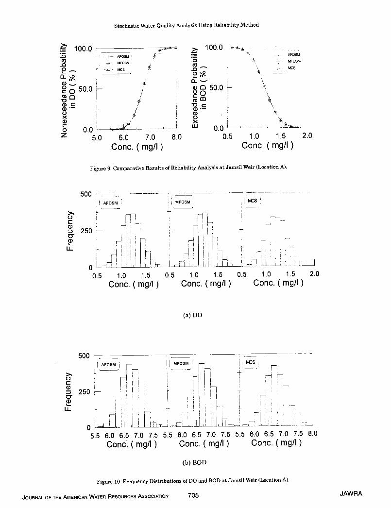
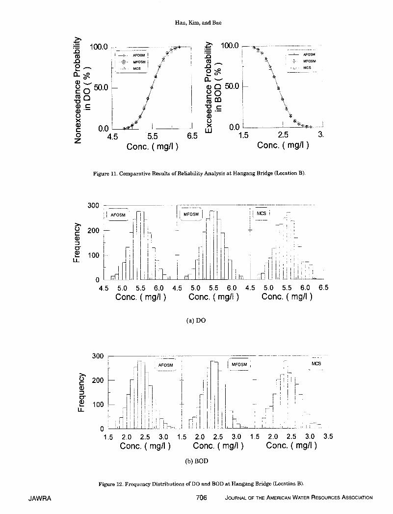
Risk analyses were performed for DO and BOD,which are generally known as the most importantwater quality control variable. As seen in Figure 3,the selected locations are just downstream of theJamsil weir (Location A) and the Hangang bridge(Location B). Figure 9 shows the results of the relia-bility analysis for DO and BOD at Location A. TheseCDFs were then used for computing the frequencydistributions, shown in Figure 10, of the output vari-ables from the three selected methods. As shown inFigures 11 and 12, the results at Location B were verysimilar to those at Location A: the ranges of DO andBOD were 5.6 to 8.0 mg/I and 0.6 to 1.8 mg/I at Loca-tion A; and 4.7 to 6.2 mg/i and 1.6 to 3.3 mg/i at Loca-tion B, respectively. Of course, the risks for all theother interesting locations on the river can also beobtained in a similar manner. Furthermore, theAFOSM, MFOSM, and Monte Carlo methods werecompared in terms of the exceedance probabilitycurves for their predictions of the lowest DO andhighest BOD at selected locations (shown in Figures 9and 11). Overall, the results from the AFOSM methodwere closer to those from the MFOSM method thanthose from the Monte Carlo simulation. The differ-ences between the three methods were minor in thecentral portion of the exceedance probability curve,yet more significant at the tails. In terms of practicaluse in this study area, the MFOSM method would


—4—— AFOSM-4 MFOSM

- MCS

L

I ____________ I

0)E

0a

d0)

0)E

a0C

d(I)

2.0

1.0

0.0

2.0

1.0

0.0

10.0 20.0 30.0 40.0Location ( km)

---i-— AOSM

-- MFOSM

MCS

10.0 20.0 30.0 40.0Location (km)

(19)

(20)

(21)

500


Figure 9. Comparative Results of Reliability Analysis at Jamsil Weir (Location A).

____ MFOSM

> L ±0 I

250— H1 +HHH H:I-

0HLH Ht

—

—H- AFOSM—

MFOSM

r --- MCS

r /-

i 100.0--0a)..—

50.0

.oa)0>(a)

o 0.0z

500

: 100.0"H.-FOSM

28°•° H

a)C)x

0.05.0 6.0

Conc.8.07.0

mg/I)0.5 1.0

Conc.2.01.5

mg/I)

>C)

a)

IL

AFOSM

250— T

0H1.O

Conc.

MFOSM

t

L H H,H I

-L

L_ --- i-I0.5 1.0 1.5 2.0

Conc. (mg/I)1.5

mg/I)0.5 1.0 1.5

Conc. (mg/I)

(a) DO

Th rTrTwHJJL1

5.5 6.0 6.5 7.0 7.5 5.5 6.0 6.5 7.0 7.5 5.5 6.0 6.5 7.0 7.5 8.0Conc. (mg/I) Conc. (mg/I) Conc. (mg/I)

(b) BOD

Figure 10. Frequency Distributions of DO and BOD at Jamsil Weir (Location A).


>0Cci)

a)I—IL

>.0Ca)

a)U-

Han, Kim, and Bae

Figure 11. Comparative Results of Reliability Analysis at Hangang Bridge (Location B).

McS

r-HH

Figure 12. Frequency Distributions of DO and BOD at Hangang Bridge (Location B).


100.0>4-.

Co-Q2—s

a).—

a).—0xa)C0z

100.0 --- -'-—4—-- AFOSM

H MFOSM COIIMc5

/50.OH- / C.)

CCoca

-

0.04.5

—-4— AFOSM

-- MFOSM----

50.0 H-

b

\.

0.0 L .1.5 2.5 3.5.5

Conc. (mg/I)6.5

Conc. (mg/I)

n' HMFOSM•-—- T

bMcs

-———---

H

H-

H-1

rni

PH-rnj

t

300

200

100

0

300

200

100

0

4.5 5.0 5.5Conc. (

6.0 4.5 5.0 5.5mg/I) Conc. (

6.0 4.5 5.0 5.5mg/I) Conc. (

6.0 6.5mg/I)

(a) DO

AFOSM

H

HI.'

hir11

J4LLL U

H

H-

r .LJ4tL

P

rirf I

1

r

H

MFOSM

1H

Li I r.1.5 2.0 2.5

Conc. (3.0 1.5 2.0 2.5

mg/I) Conc. (3.0 1.5 2.0 2.5

mg/I) Conc. (3.0 3.5

mg/I)

(b) DOD


seem to be the most appropriate when considering itscomputational simplicity and shorter execution time.

SUMMARY AND CONCLUSIONS

This study developed a QUAL2E-RA (QUAL2E -Reliability Analysis) model for the stochastic waterquality analysis at the Han River in Korea. TheQUAL2E-RA model is based on QUAL2E-UNCAS,that has an uncertainty analysis option based on theMonte Carlo simulation method. Because the MonteCarlo simulation requires a large computation effort,the AFOSM and MFOSM methods are incorporatedinto QUAL2E-RA. After identifying the hydrauliccharacteristics using a standard step method, theoptimal reaction coefficients are calibrated using theBFGS optimization technique. A stochastic waterquality analysis is then performed for the study area.

It was found that the reaction coefficients relatingto DO and BOD were sensitive to the model perfor-mance in the study area, while those for T-N and T-Pwere not. In particular, DO and BOD were sensitiveto the BOD deoxygenation rate, k1, the loss rate ofBOD due to settling, k3, and the sediment oxygendemand rate, k4. The optimal coefficients for k1, k3,and k4 were calibrated for the upstream and down-stream parts of the Jamsil weir. It was also foundthat the results computed for DO and BOD were ingood agreement with the measured values being thecorrelation coefficient is greater than 0.95.

The statistical results from a comparative study ofthree uncertainty analysis methods showed that theestimated water quality variables from the AFOSMand MFOSM methods were similar to those from theMonte Carlo method. Also, the frequency distribu-tions and the corresponding reliabilities obtainedfrom all three methods were very close to each other.In terms of the model accuracy, all three methodswould appear to be equally appropriate for use in aprobabilistic water quality management system in thestudy area, when they are optionally used as a compo-nent of QUAL2E-RA. However, the AFOSM andMFOSM methods have an advantage in that they donot require a large computation time to achieve thesame quality of reliability analysis, although themathematical formulations of the AFOSM andMFOSM methods are more or less complicate thanthat of the Monte Carlo technique. From a practicalmodel selection perspective, the MFOSM method ismore attractive due to its lower computational com-plexity and less execution time. It can be concludedthat the proposed stochastic water quality model canbe useful for scientific water quality planning andmanagement.

ACKNOWLEDGEMENTS

The research for this paper was supported by the Korea Scienceand Engineering Foundation under Grant No. KOSEF 98-0601-04-01-3. The thoughtful comments of anonymous reviewers of a previ-ous version of this paper are gratefully acknowledged.

LITERATURE CITED

Ang, A. H. and W. H. Tang, 1984. Probability Concepts in Engineer-ing Planning and Design. Volume II, John Wiley and Sons.

Brown, R. T. and T. 0. Barnwell, 1987. The Enhanced StreamWater Quality Model QUAL2E and QUAL2E-UNCAS. EPAI600-3-87/007, U.S. Environmental Protection Agency.

Burges, S. J. and D. P. Lettenmaier, 1975. Probabilistic Methods inStream Quality Management. Water Resources Bulletin11( 1): 115-130.

Chadderton, R. A., A. C. Miller, and A. J. McDonnell, 1982. Uncer-tainty Analysis of Dissolved Oxygen Models. Journal of Environ-mental Engineering Division, ASCE 198(EE5):1003-1011.

Chapra, S. C., 1997. Surface Water Quality Modeling. McGraw-Hill,pp. 317-343.

Chaudhry, M. H., 1993. Open Channel Flow. Prentice-Hall, pp. 133-137.

City of Seoul, 1992. Flood Management Study in the MetropolitanSeoul Area (in Korean).

Dennis, J. E., Jr. and J. J. More, 1977. Quasi-Newton Methods,Motivation and Theory. SIAM Rev. 19, No. 1.

Kothandaraman, V. and B. B. Ewing, 1969. A Probabilistic Analysisof DO-BOD Relationships in Stream. Journal of Water PollutionControl Federation 41(2):R73-R90.

Kuo, J. T., A. Y. Kuo, and W. S. Chung, 1997. Water Quality Model-ing and Risk Analysis of the Keelung River. Managing Water:Coping with Scarcity and Abundance. ASCE, pp. 441-446.

Melching, C. S. and S. Anmangandla, 1992. Improved First-OrderUncertainty Method for Water-Quality Modeling. Journal ofEnvironmental Engineering, ASCE 118(EE5):791-805.

MOE (Ministry of Environment), 1985-1994. Water Quality Mea-surement Data. Ministry of Environment.

Qaisi, K., 1988. Stochastic Modeling of Dissolved Oxygen inStreams. Computer Methods and Water Resources: Water Quali-ty, Planning and Management. Springer-Verlag, pp. 173-182

Rackwitz, R., 1976. Practical Probabilistic Approach to Design. Bul-letin No. 112, Comite European du Beton, Paris, France.

Rackwitz, R. and B. Fiessler, 1977. Non-Normal Distributions inStructural Reliability. SFB 96, Report 29, Technical Universityof Munich, pp. 1-22.

Schnoor, J. L., 1996. Environmental Modeling, John Wiley andSons, pp. 259-270.

Streeter, H. W. and E. B. Phelps, 1925. A Study on the Pollutionand Natural Purification of the Ohio River, III. Factors Concern-ing the Phenomena of Oxidation and Reaeration. U.S. PublicHealth Service, Public Health Bulletin, No. 146.

Tung, Y. K. and W. E. Hathhorn, 1988. Assessment of ProbabilityDistribution of Dissolved Oxygen Deficit. Journal of Environ-mental Engineering, ASCE 114(EE6):1421-1435.

Vanderplaats, G. N., 1984. Numerical Optimization Techniques forEngineering Design. McGraw-Hill.

Vasquez, J. A., H. R. Maier, B. J. Lence, B. A. Tolson, and R. 0. Fos-chi, 2000. Achieving Water Quality System Reliability UsingGenetic Algorithms. Journal of Environmental Engineering,ASCE 126(10): 954-962.

Warwick, J. J., 1997. Use of First-Order Uncertainty Analysis toOptimize Successful Stream Water Quality Simulation. Journalof American Water Resources Association 33(6):1173-1185.


Han, Kim, and Bae

Warwick, J. J. and W. G. Cale, 1987. Determining of Likelihood of13 reliability index.

Obtaining a Reliable Model. Journal of Environmental Engi-neering, ASCE 112(EE5): 1102-1119. ii) = standard normal mtegral.

Yen, B. C., S. T. Cheng, and C. S. Melching, 1986. First Order Relia- = the difference between two iterations.bility Analysis. In: Stochastic and Risk Analysis in HydraulicEngineering, B. C. Yen (Editor). Water Resource Publications,Littleton, Colorado, pp. 1-36.

NOTATIONS

C = partial derivative of system performance function withrespect to basic variable i.

C8 = a base value of water quality concentration.

C1 = the lower value of water quality concentration.

C = the upper value of water quality concentration.

e1 = the relative error of the computed water quality data.

El I = expectedor mean value of random variable.

g = acceleration due to gravity.

go = system performance function.

G = inverse of the Hessian matrix.

h = depth of flow.

hf = friction loss head.

H = totalhead.

= iteration number.

k1 = biochemical oxygen demand(BOD) deoxygenation rate.

k3 = loss rate of BOD due to settling.

= sediment oxygen demand rate.

L = load in reliability analysis.

n = number of variables/simulations, or parameter vector.

o = observed value of water quality variable.

= exceedance probability.

Pf = probability of failure.

Q = discharge.

R = resistance in reliability analysis.S = sum of squared error.

Sc = friction slope.

U = velocity.

Ax = distance in space.

X1 = value of basic variable i.* . .xj = value of basic vanable i atfailure surface.

= mean value of basic variable i.

= computed value of water quality variable.

z = watersurface elevation above datum.

Z = performance variable.


Documents

STOCHASTIC WATER QUALITY ANALYSIS USING RELIABILITY METHOD