Embed Size (px)
Citation preview

Stock Price Prediction & Optimal Portfolio Selection using
Signal Processing
A Project Report
submitted by
NISHIDH BIYANI
in partial fulfillment of the requirements
for the award of the degree of
DUAL DEGREE IN ELECTRICAL ENGINEERING
DEPARTMENT OF ELECTRICAL ENGINEERING
INDIAN INSTITUTE OF TECHNOLOGY MADRAS.
MAY 2013

THESIS CERTIFICATE
This is to certify that the thesis titled STOCK PRICE PREDICTION & OPTIMAL
PORTFOLIO SELECTION USING SIGNAL PROCESSING, submitted by NISHIDH
BIYANI, to the Indian Institute of Technology Madras, Chennai for the award of the degree of
Masters in Electrical Engineering, is a bona fide record of the research work done by him
under our supervision. The contents of this thesis, in full or in parts, have not been submitted to
any other Institute or University for the award of any degree or diploma.
Dr. Bharath Bhikkaji
Research Guide
Professor
Department of Electrical Engineering Place: Chennai
IIT-Madras, 600 036
Date: 7th
May 2013

i
ACKNOWLEDGEMENTS
It is indeed a great privilege for me to present this work, I take this opportunity to thank
all those who made this endeavor a success.
Foremost, I would like to express my gratitude to my advisor Prof. Bharath Bhikkaji for
the continuous support, innumerable suggestions, good guidance and cooperation, right from the
beginning and during the project. I am fortunate to work under him.
I thank the team of Santa Fe Research- Arun, Jerin and Shravan who helped and
contributed great ideas and advices. I also thank Dr. Girish Ganesan for his support and
guidance.
Lastly, I thank my parents for giving constant support and encouragement to pursue my
studies.

ii
ABSTRACT
KEYWORDS: HMM, Gaussian Mixture Models, CRP, Universal Portfolio Theory,
Commission, Side Information.
Stock market analysis and prediction is one of the interesting areas in which past data
could be used to anticipate and predict information about future. Technically speaking, this area
is of high importance for professionals in the industry of finance and stock exchange as they can
lead and direct future trends or manage crises over time. In this assignment, we try to take
advantage of Hidden Markov Models (HMM) to address some interesting problems regarding
stock market analysis. Specifically, stock price prediction is done in this assignment. First, a set
of past data is loaded and analyzed; then, an HMM is modeled and trained for the problem
model. Afterwards, similar past data are distinguished and used to predict future stock market
values. Stock market data that are used in this assignment are the data from NSE (National Stock
Exchange). Basically, each stock market data is a quadruple (open; low; high; close) carrying the
meaning that each day the stock market starts its activity, it starts with some opening after which
during the day it reaches its highest or drops down to its lowest of the day and then it will stop
with a close value. Such data seems to be very sensitive for stock traders and business
shareholders to predict future stock trends. In this assignment, we try to estimate the future day's
close values as precisely as possible.
This project also deals with the portfolio theory developed by Thomas M. Cover. Our
main goal is to understand the link of information theory to the theory of optimal investments in
a stock market. Firstly, we analyze the Constant Rebalanced Portfolio Theory (CRP) given by
Cover. A CRP is an investment strategy which keeps the same distribution of wealth among a set
of stocks from period to period. That is, the proportion of total wealth in a given stock is the
same at the beginning of each period. It is proven that CRP is the best portfolio strategy and no
other portfolio strategy can outperform it. But there are some practical issues in implementing
CRP in real stock market. To overcome these issues, Cover gave Universal Portfolio Theory
which asymptotically performs same as CRP and is more practically feasible. We analyze the
Universal Portfolio Theory and simulate it on a two stock portfolio.

iii
The Universal Portfolio Theory does not take into account transaction fees, which
could be the bane for an investor as according to the Universal Portfolio Theory portfolio has to
be updated daily. We provide a simple analysis which naturally extends to the case of a fixed
percentage transaction cost (commission). In addition, we present a simple implementation on
real stock market. Inclusion of transaction costs in the Universal Portfolio Theory makes it the
best and practically feasible portfolio strategy on paper. But the market varies in such a manner
that there is possibility of outperforming this strategy by having insightful information about the
market. Portfolio management based on instincts and extra information can outperform this, but
algorithmically it is the best strategy. It requires no extra information and no expertise on stock
market. Any person with no expertise in stock market can use this strategy and get way better
returns than any other strategies available to him.
Lastly, we tried to incorporate extra information (side information) or credible
expert opinion into our algorithm to improve our returns. We worked on state constant
rebalanced portfolio and clubbed the same concept with the universal portfolio to use the side
information. In our case we looked into stocks listed on both NYSE and NSE. And used the
performance of the stocks on NYSE as the side information and updated the portfolio in NSE
accordingly. This surpasses the returns of the universal portfolio without side information. We
also looked into the upper bound on the increment in the returns due to the side information. The
increment in the returns resulting from the side information is upper-bounded by the mutual
information between the stock vector and the side information.

iv
TABLE OF CONTENTS
ACKNOWLEDGEMENTS i
ABSTRACT ii
LIST OF FIGURES vi
ABBREVIATIONS vii
CHAPTER 1. STOCK PRICE PREDICTION USING HMM 1
1.1 Introduction to Markov Models …………………………………
1.2 Hidden Markov Models…………………………………………
1.2.1 Three fundamental problems for HMMs………
1.2.2 The Forward Algorithm………………………
1.2.3 The Backward Algorithm………………………
1.2.4 Baum Welch Algorithm………………………
1.3 HMM as a Predictor………………………………………………
1.4 Implementation…………………………………………………
1.4.1 HMM Parameters…………………………….
1.4.2 Initialization………………………………….
1.4.3 Prediction…………………………………….
1.5 Results………………………………………………………….
CHAPTER 2. LOG OPTIMAL PORTFOLIO 15
2.1 Stock market, Portfolio and Wealth………………………………
2.2 Growth Rate and Log-optimal Portfolio……………………….
2.3 Kuhn-Tucker Characterization of the Log-optimal Portfolio………
2.4 Asymptotic Optimality of the Log-optimal Portfolio………………

v
CHAPTER 3. UNIVERSAL PORTFOLIO THEORY 26
3.1 Universal Portfolio Theory without Commission………………
3.2 Universal Portfolio with Commission ………………………….
3.3 Implementation and Results…………………………………….
CHAPTER 4. SIDE INFORMATION 32
4.1 Side Information and the Doubling Rate………………………
4.2 State Constant Rebalanced Portfolios……………………………
4.3 Example explaining impact of Side Information………………….
4.4 Universal Portfolio with Side Information………………………
4.5 Implementation on real Stock market……………………………
REFERENCES 40

vi
LIST OF FIGURES
1.1. The Forward Procedure…………………………………………………………………. 4
1.2. The Backward Procedure……………………………………………………………… 5
1.3. Plot comparing the Predicted Closing Price to the Actual Closing Price for IBM…… 12
1.4. Plot comparing the Predicted Closing Price to the Actual Closing Price for Dell…… 12
1.5. Plot comparing the Predicted Closing Price to the Actual Closing Price for Southwest
Airlines………………………………………………………………………………… 13
1.6. Plot comparing the Predicted Closing Price to the Actual Closing Price for Ryanair
Holdings……………………………………………………………………………… 13
1.7. Plot comparing the Predicted Closing Price to the Actual Closing Price for Apple Inc. 14
2.1. Sharpe Markowitz Theory 16
3.1. Comparing the results of Universal Portfolio Strategy with other strategies…………… 30
3.2. Effect of Transaction Cost on the returns of Universal Portfolio Theory……………… 31
4.1. Comparison of Universal Portfolio with and without Side Information……………… 39
vii
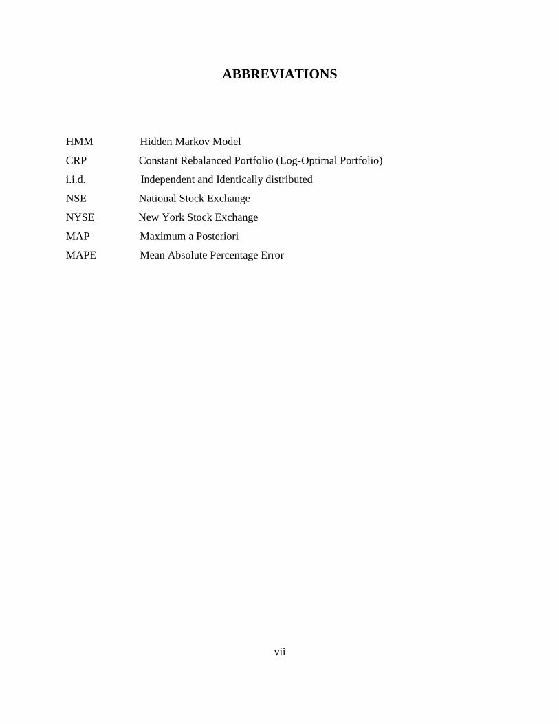
ABBREVIATIONS
HMM Hidden Markov Model
CRP Constant Rebalanced Portfolio (Log-Optimal Portfolio)
i.i.d. Independent and Identically distributed
NSE National Stock Exchange
NYSE New York Stock Exchange
MAP Maximum a Posteriori
MAPE Mean Absolute Percentage Error
1
CHAPTER 1
STOCK PRICE PREDICTION USING HMM
Stock market analysis and prediction is one of the interesting areas in which past data
could be used to anticipate and predict information about future. Technically speaking, this area
is of high importance for professionals in the industry of finance and stock exchange as they can
lead and direct future trends or manage crises over time. In this assignment, we try to take
advantage of Hidden Markov Models (HMM) to address some interesting problems regarding
stock market analysis. Specifically, stock price prediction is done in this assignment. Hidden
Markov models are especially known for their application in temporal pattern recognition such
as speech, handwriting, gesture recognition. A hidden Markov model can be considered a
generalization of a mixture model where the hidden variables, which control the mixture
component to be selected for each observation, are related through a Markov process rather than
independent of each other.
1.1 Introduction to Markov Models
Markov models are used to train and recognize sequential data, such as speech utterances,
temperature variations, biological sequences, and other sequence data. In a Markov model, each
observation in the data sequence depends on previous elements in the sequence. Consider a
system where there are a set of distinct states { }. At each discrete time slot t, the
system moves to one of the states according to a set of state transition probabilities . We denote
the state at time t as . Since the state transition is independent of time, we can have the
following state transition matrix :
is state transition probability, hence:
∑
2
Also we need to know the probability to start from a certain state, the initial state distribution:
Therefore, ∑ .
1.2 Hidden Markov Models
A HMM is a doubly stochastic process with an underlying stochastic process that is not
observable (it is hidden), but can only be observed through another set of stochastic processes
that produce the sequence of observed symbols. In an HMM, one does not know anything about
what generates the observation sequence. The number of states, the transition probabilities, and
from which state observation is generated all are unknown. Each state of the HMM is associated
with a probabilistic function. At time , an observation is generated by a probabilistic
function , which is associated with state , with the probability:
A HMM is composed of five tuple:
{ } is the set of states. The state at time is denoted by .
number of distinct observation symbols per state (observation symbols correspond
to the physical output of the system being modeled)
Initial state distribution { } is defined as
State transition probability distribution { } .
Observation symbol probability distribution . The probabilistic function for
each state is :

3
The overall HMM model is denoted by
After modeling a problem as an HMM, and assuming that some set of data was generated
by the HMM, we are able to calculate the probabilities of the observation sequence and the
probable underlying state sequences. Also we can train the model parameters based on the
observed data and get a more accurate model. Then use the trained model to predict unseen data.
1.2.1 Three Fundamental Problems for HMMs
1. Given the model how do we compute , the probability of
occurrence of the observation sequence .
2. Given the observation sequence and a model , how do we choose a state sequence
that best explains the observations.
3. Given the observation sequence and a space of models found by varying the model
parameters , and , how do we find the model that best explains the observed
data.
There are established algorithms to solve the above questions [3]. In our task we have
used the forward-backward algorithm to compute the and Baum-Welch algorithm to
train the HMM.
1.2.2 The Forward Algorithm
The forward variable is defined as:
stores the total probability of ending up in state at time , given the observation sequence
.

4
Fig.1.1 – The Forward Procedure
The forward procedure:
1. Initialization
2. Induction
[∑
]
3. Update time by setting ; Return to step 2 if ; Otherwise, terminate
algorithm
4. Termination
∑

5
1.2.3 The Backward Algorithm
The backward procedure calculates the probability of the partial observation sequence
from to the end, given the model and state at time . The backward variable is
defined as:
The backward procedure:
1. Initialization
2. Induction
∑
3. Update time by setting ; Return to step 2 if ; Otherwise terminate the
algorithm
4. Termination
∑
Fig.1.2 – The Backward Procedure

6
1.2.4 Baum Welch Algorithm
The last and most difficult problem about HMMs is that of parameter estimation. Given
an observation sequence, we want to find the model parameters that best explains
the observation sequence. The problem can be reformulated as find the parameters that maximize
the following probability:
There is no known analytic method to choose to maximize but we can use a
local maximization algorithm to find the highest probability. This algorithm is also called the
Baum Welch. It is a special case of the Expectation Maximization method [1]. It works
iteratively to improve the likelihood of . This iterative process is called the training of the
model. The Baum-Welch algorithm is numerically stable with the likelihood non-decreasing of
each iteration. It has linear convergence to a local optima.
To work out the optimal model iteratively, we will need to define a few
intermediate variables. Define as follows:
∑
∑ ∑
This is the probability of being at state at time , and at state at time , given the model
and the observation .

7
Then define . This is the probability of being at state at time , given the observation and
the model :
∑
∑
The above equation holds because is the expected number of transition from state
and is the expected number of transitions from state to .
Given the above definitions we begin with an initial model and run the training data
through the current model to estimate the expectations of each model parameter. Then we can
change the model to maximize the values of the paths that are used. By repeating this process we
hope to converge on the optimal values for the model parameters.
The re-estimation formulas of the model are:
∑
∑

8
∑
∑
1.3 HMM as a Predictor
We use a continuous Hidden Markov Model to model the stock data as a time series. An
HMM can be written as . Where is the transition matrix whose elements give the
probability of a transition from one state to another, is the emission matrix giving the
probability of observing when in state , and gives the initial probabilities of the states
at . Further for a continuous HMM the emission probabilities are modeled as Gaussian
Mixture Models (GMMs):
∑ )
where:
is the number of Gaussian Mixture components.
is the weight of the mixture component in state .
is the mean vector for the component in the state.
is the probability of observing vector in the multi-dimensional
Gaussian distribution.
is the Covariance matrix for the mixture component in state
Training of the above HMM from given sequences of observations is done using the
Baum-Welch algorithm which uses Expectation-Maximization (EM) to arrive at the optimal
parameters for the HMM. In our model the observations are the daily stock data in the form of
the 4-dimensional vector,
(
)

9
Here open is the day opening value, close is the day closing value, high is the day high, and low
is the day low. We use fractional changes along to model the variation in stock data which
remains constant over the years [4].
Once the model is trained, testing is done using an approximate Maximum a Posteriori
(MAP) approach. We assume a latency of days while forecasting future stock values. Hence,
the problem becomes as follows - given the
HMM model and the stock values for days along with the stock open value
for the day, we need to compute the close value for the day. This is
equivalent to estimating the fractional change
for the day. For this, we
compute the MAP estimate of the observation vector .
Let be the MAP estimate of the observation on the day, given the values
of the first days. Then,
The observation vector is varied over all possible values. Since the denominator is
constant with respect to , the MAP estimate becomes,
The joint probability value can be computed using the forward-
backward algorithm for HMMs. In practice, we compute the probability over a discrete set of
possible values of and find the maximum. The computational complexity of the forward-
backward algorithm for finding the likelihood of a given observation is , where is the
number of states in the HMM and is the latency. This procedure is repeated over the discrete
set of possible values of . In our case and there are possible

10
values of . The closing value of a particular day can be computed by using the day opening
value and the predicted fractional change for that day.
1.4 Implementation
1.4.1 HMM Parameters
The HMM parameters are set to the following values:
Number of underlying Hidden States
Number of mixture components for each state
Dimension of observations
Ergodic HMM (all transitions are possible).
Latency days.
These were obtained by varying the parameters over suitable ranges and choosing the values
which give the minimum error between forecasted and actual stock values [2].
1.4.2 Initialization
For initialization of the model parameters the prior probabilities and transition
probabilities are assumed to be uniform across all states. To initialize the mean, variance and
weights of the Gaussian mixture components we use k-means algorithm. Each cluster found from
k-means is assumed to be a separate mixture component from which the mean and variance are
computed. Weights of the components are assumed to be weights of the clusters, which are
divided equally between the states to obtain the initial emission probabilities.
1.4.3 Prediction
To compute the MAP estimate , we compute the probability values over a range of
possible values of the tuple
and find the maximum. A higher
precision is used for the fractional change values since these are ultimately used for the stock
prediction. The range of values is listed in table below.
11
Observation Range Number of Points
Min. Max.
-0.1 0.1 50
0 0.1 10
0 0.1 10
1.5 Results
The metric used to evaluate the performance of the algorithm is Mean Absolute
Percentage Error (MAPE) in accuracy. MAPE is the average absolute error between the actual
stock values and the predicted stock values in percentage.
∑
where is the actual stock value, is the predicted stock value on day and is the number of
days for which the data is tested. The table below lists the MAPE values for the four stocks using
our developed algorithm.
Stock Name MAPE
IBM 1.067%
Dell 1.654%
Southwest Airlines 1.857%
Ryanair Holdings 1.944%
Apple Inc. 6.057%

12
We took 1 year data for training the model and predicted the closing price for next 90 days. The
following plots compare the predicted closing price for the above mentioned 5 stocks with the
actual closing price for that day.
Fig.1.3 – Plot comparing the Predicted Closing Price to the Actual Closing Price for IBM
Fig.1.4 – Plot comparing the Predicted Closing Price to the Actual Closing Price for Dell
75
80
85
90
95
100
105
1 5 9 13 17 21 25 29 33 37 41 45 49 53 57 61 65 69 73 77 81 85
Sto
ck P
rice
fo
r IB
M
Prediction Day
Stock Price Prediction for IBM
Actual Closing Price
Predicted Closing Price
0
5
10
15
20
25
30
35
40
45
1 5 9 13 17 21 25 29 33 37 41 45 49 53 57 61 65 69 73 77 81 85
Sto
ck P
rice
fo
r D
ell
Prediction Day
Stock Price Prediction for Dell
Actual Closing Price
Predicted Closing Price

13
Fig.1.5 – Plot comparing the Predicted Closing Price to the Actual Closing Price for Southwest
Airlines
Fig.1.6 – Plot comparing the Predicted Closing Price to the Actual Closing Price for Ryanair
Holdings
0
2
4
6
8
10
12
14
16
18
1 5 9 13 17 21 25 29 33 37 41 45 49 53 57 61 65 69 73 77 81Sto
ck P
rice
fo
r So
uw
est
Air
line
s
Prediction Day
Stock Price Prediction for Southwest Airlines
Actual Closing Price
Predicted Closing Price
0
10
20
30
40
50
60
1 4 7 10 13 16 19 22 25 28 31 34 37 40 43 46 49 52 55 58 61 64 67 70Sto
ck P
rice
fo
r R
yan
air
Ho
ldin
gs
Prediction Day
Stock Price Prediction for Ryanair Holdings
Actual Closing Price
Predicted Closing Price

14
Fig.1.7 – Plot comparing the Predicted Closing Price to the Actual Closing Price for Apple Inc.
For above results we took non-volatile stocks in a very stable market situation. The
problem with the proposed model is that it does not take into account changes in the market due
to unpredictable and unquantifiable factors such as, policies, market conditions etc. This model
entirely depends on the past training data and it is not always necessary that stock prices follow
the same trend as it did in past, which is quite visible in the stock prediction plot for Apple Inc.
For other 4 stocks it approximately predicted the stock price, but for Apple it did not. Stock Price
is not only a function of past prices in real market.
This is a very basic model which approaches the problem of stock price prediction using
HMM. The model can be improved by giving some meaning to the states defined. To give
meaning to state one should analyze the stock market and try to define the states in a different
manner.
In the current approach, we also assumed that the model for one particular stock is
independent of the other stocks in the market, however in reality these stocks are heavily
correlated to each other and, to some extent, to stocks in other markets too. As a future work, it
might be intuitive to try and build a model which takes into consideration these correlations.
Also, currently the data is quantized to form observation vectors for a full day. A performance
improvement might be achieved by removing this quantization and instead taking the full range
of minute-by-minute or hour-by-hour stock values.
0
10
20
30
40
50
60
70
80
1 5 9 13 17 21 25 29 33 37 41 45 49 53 57 61 65 69 73 77 81 85Sto
ck P
rice
Pre
dic
tio
n f
or
Ap
ple
Inc.
Prediction Day
Stock Price Prediction for Apple Inc.
Actual Closing Price
Predicted Closing Price

15
CHAPTER 2
LOG-OPTIMAL PORTFOLIO THEORY
The duality between the growth rate of wealth in the stock market and the entropy rate of
the market is striking. In particular, we shall find the competitively optimal and growth rate
optimal portfolio strategies. They are the same, just as the Shannon code is optimal both
competitively and in expected value in data compression. We shall also find the asymptotic
doubling rate for an ergodic stock market process. I would like to remark that the portfolio
theory based on Information Theory is completely adapted from the work done in this field by
Thomas M. Cover and Joy A. Thomas [10].
2.1 Stock Market, Portfolio and Wealth
Definition 2.1 A stock market is a random return vector,
where, is the number of stocks in the stock market, is the price relative or return of stock
i.e., the ratio of the price at the end of the day to the price at the beginning of the day and
is the joint distribution of the vector of price relatives.
Definition 2.2 A portfolio is a vector,
∑

16
Where, is the portfolio weights i.e., the fraction of the investor's capital in stock .
Definition 2.3 Let be a portfolio and a stock market, the resulting random wealth (relative)
at the end of the day is
∑
We wish to maximize in some sense. But is a random variable, so there is controversy
over the choice of the best distribution for S. The standard theory of stock market investment is
based on the consideration of the first and second moments of S. The objective is to maximize
the expected value of S, subject to a constraint on the variance. Since it is easy to calculate these
moments, the theory is simpler than the theory that deals with the entire distribution of S. The
mean-variance approach is the basis of the Sharpe-Markowitz theory of investment in the stock
market and is used by business analysts and others [11]. The figure 2.1 illustrates the set of
achievable mean-variance pairs using various portfolios. The set of portfolios on the boundary of
this region corresponds to the un-dominated portfolios: these are the portfolios which have the
highest mean for a given variance. This boundary is called the efficient frontier, and if one is
interested only in mean and variance, then one should operate along this boundary.
Fig.2.1 – Sharpe Markowitz Theory

17
Normally the theory is simplified with the introduction of a risk-free asset, e.g., cash or
Treasury bonds, which provide a fixed interest rate with variance 0. This stock corresponds to a
point on the Y axis in the figure. By combining the risk-free asset with various stocks, one
obtains all points below the tangent from the risk-free asset to the efficient frontier. This line
now becomes part of the efficient frontier. The concept of the efficient frontier also implies that
there is a true value for a stock corresponding to its risk. This theory of stock prices is called the
Capital Assets Pricing Model and is used to decide whether the market price for a stock is too
high or too low.
2.2 Growth Rate and Log-optimal Portfolio
Our objective is to find the largest wealth . To motivate this, we define the growth rate
and the log-optimal portfolio. Looking at the mean of a random variable gives information about
the long term behavior of the sum of i.i.d. versions of the random variable. But in the stock
market, one normally reinvests every day, so that the wealth at the end of n days is the product of
factors, one for each day of the market. The behavior of the product is determined not by the
expected value but by the expected logarithm. This leads us to define the doubling rate as
follows:
Definition 2.4 The growth rate of a portfolio with respect to a stock distribution is the
expected value of the logarithm of wealth,
∫
The reason why we do not define the growth rate as , is the multiplicative growth of
wealth Assume that one invests days. The resulting wealth at the end of days would be
∏
18
According to the strong law of large numbers, the expected value of describe the dominant
behavior of ∏ i.e., ∏
⁄
Definition 2.5 The optimal doubling rate is defined as
Where, the maximum is over all possible portfolios ∑
Definition 2.6 A portfolio that achieves the maximum of is called a log optimal
portfolio.
The definition of doubling rate is justified by the following theorem,
Theorem 2.1 Let be i.i.d. according to . Let
∏
Be the wealth after days using the constant rebalanced portfolio . Then
with probability 1.
Proof:
∑
with probability 1,
by the strong law of large numbers. Hence,
Lemma 2.1 is concave in and linear in . is convex in
Proof: The doubling rate is

19
∫ .
Since the integral is linear in so is .
Since
by the concavity of the logarithm, it follows, by taking expectations, that is concave
in .
Finally, to prove the convexity of as a function of , let and be two
distributions on the stock market and let the corresponding optimal portfolios be
and respectively. Let the log-optimal portfolio corresponding to
be . Then by linearity of with respect to we have
,
Since maximizes and maximizes .
Lemma 2.2 The set of log-optimal portfolios forms a convex set.
Proof: Let and
be any two portfolios in the set of log-optimal portfolios. By the previous
lemma, the convex combination of and
has a doubling rate greater than or equal to the
doubling rate of or
, and hence the convex combination also achieves the maximum
doubling rate. Hence the set of portfolios that achieves the maximum doubling rate. Hence the
set of portfolios that achieves the maximum is the convex.

20
2.3 Kuhn-Tucker Characterization of the Log-optimal Portfolio
The determination that achieves is a problem of maximization of a concave function
over a convex set . The maximum may lie on the boundary.
Theorem 2.2 The log-optimal portfolio for a stock market , i.e., the portfolio that
maximizes the doubling rate , satisfies the following necessary and sufficient conditions:
(
) if
(
) if
Proof: The doubling rate is concave in , where ranges over the simplex
of portfolios. It follows that is log-optimum iff the directional derivative of in the
direction from to any alternative portfolio is non-positive. Thus, letting
for , we have
.
These conditions can be reduced since the one-sided derivative at of is
(
)
(
( (
)))
(
) ,

21
where the interchange of limit and expectation can be justified using the dominated convergence
theorem. Thus
(
)
for all .
If the line segment from to can be extended beyond in the simplex, then the two-
sided derivative at of vanishes and the above equation holds with equality. If the
line segment from to cannot be extended, then we have an inequality in the above equation.
This theorem has a few immediate consequences. One surprising result is expressed in
the following theorem:
Theorem 2.3 Let be the random wealth resulting from the log-optimal portfolio .
Let be the wealth resulting from any other portfolio . Then
(
)
Conversely, if (
) for all portfolios , then * (
)+ for all .
This theorem can be stated more symmetrically as
* (
)+ for all
⇔ (
) , for all .
Proof: From the previous theorem, it follows that for a log-optimal portfolio ,
(
)
for all . Multiplying this equation by and summing over , we have

22
∑ (
) ∑
which is equivalent to
(
) (
) .
The converse follows from Jensen’s inequality, since
* (
)+ (
) .
Thus expected log ratio optimality is equivalent to expected ratio optimality.
Maximizing the expected algorithm was motivated by the asymptotic growth rate. But we
have shown that the log- optimal portfolio, in addition to maximizing the asymptotic growth rate,
also maximizes the wealth relative for one day.
Another consequence of Kuhn-Tucker characterization of the log-optimal portfolio is the
fact that the expected proportion of wealth in each stock under the log-optimal portfolio is
unchanged from day to day. Consider the stocks at the end of first day. The initial allocation of
wealth is . The proportion of the wealth in stock at the end of the day is ⁄ , and the
expected value of this proportion is
(
)
(
)
Hence the expected proportion of wealth in stock at the end of the day is same as the proportion
invested in stock at the beginning of the day.
2.4 Asymptotic Optimality of the Log-optimal Portfolio
In this section we prove that with probability 1, the conditionally log-optimal investor will not do
any worse than any other investor who uses a casual investment strategy.

23
We first consider an i.i.d. stock market, i.e., are i.i.d. according to .
Let
∏
be the wealth after days for an investor who uses portfolio on day Let
be the maximal doubling rate and let be a portfolio that achieves the maximum doubling rate.
We only allow portfolios that depend casually on the past and are independent of the
future values of the stock market.
From the definition of , it immediately follow that the log-optimal portfolio
maximizes the expected log of the final wealth. This is stated in the following lemma.
Lemma 2.3 Let be the wealth after days for the investor using the log-optimal strategy on
i.i.d. stocks, and let be the wealth of any other investor using a causal portfolio strategy
Then
Proof:
∑
∑

24
∑
,
and the maximum is achieved by a constant portfolio strategy .
So far, we have proved two simple consequences of the definition of log optimal
portfolios, i.e., that maximizes the expected log wealth and that the wealth is equal to first
order in the exponent, with high probability.
Now, we will prove that exceeds the wealth (to first order in the exponent) of any
other investor for almost every sequence of outcomes from the stock market.
Theorem 2.4 Let be a sequence of i.i.d stock vectors drawn according to
Let ∏
, where is the log-optimal portfolio, and let ∏
be the
wealth resulting from any other causal portfolio. Then
with probability 1.
Proof: From the Kuhn-Tucker conditions, we have
.
Hence by Markov’s inequality, we have
(
)
.
Hence
.
25
Setting and summing over , we have
∑
∑
.
Then, by the Borel-Cantelli lemma,
infinitely often .
This implies that for almost every sequence from the stock market, there exists an such that for
all
. Thus
with probability .
The theorem proves that the log-optimal portfolio will do as well or better than any other
portfolio to first order in exponent.
The remaining question, how we can compute the log-optimal portfolio, can be solved by
the following algorithm.
Algorithm 2.1 Generate a sequence of portfolio vectors recursively according to
where . The sequence { } remains in the simplex and converges to the log-optimal
portfolio
The biggest drawback of the above algorithm is that it requires the knowledge of the
return distribution which is generally not available. The accuracy of log-optimal portfolio
depends on the accuracy of the distribution, which is very difficult to predict with high accuracy.
Hence, Cover proposed alternative portfolio theory, Universal Portfolio Theory, which gives
asymptotically same results as log-optimal portfolio.

26
CHAPTER 3
UNIVERSAL PORTFOLIO THEORY
In the previous chapter we saw that finding out the best constant ratio for the investment
according to CRP is practically infeasible. In this chapter, we give a simple analysis of the
universal algorithm of Cover, without commission. We also look into a strategy which takes
commission into account and foretells us the feasibility of investment according to Universal
Portfolio Theory [7].
3.1 Universal Portfolio Theory without Commission
Let us first consider an easier question. Suppose we just want a strategy that is
competitive with respect to the best single stock. In other words, we want to maximize the worst-
case ratio of our wealth to that of the best stock. In this case, a good strategy is simply to divide
our money among the stocks and let it sit. We will always have at least times as much
money as the best stock. Note that this deterministic strategy achieves the expected wealth of the
randomized strategy that just places all its money in a random stock. Now consider the problem
of competing with the best CRP. Cover's universal portfolio algorithm is similar to the above. It
splits its money evenly among all CRPs and lets it sit in these CRP strategies. (It does not
transfer money between the strategies.) Likewise, it always achieves the expected wealth of the
randomized strategy which invests all its money in a random CRP.
The proposed universal adaptive portfolio strategy is the performance weighted strategy
specified by
(
)
∫
∫

27
And the integration is over the set of dimensional portfolios
{ ∑
}
The wealth resulting from the universal portfolio is
∏
Thus the initial universal portfolio is uniform over the stocks, and the portfolio at time is
the performance weighted average of all portfolios .
3.2 Universal Portfolio with Commission
One of the biggest limitations of Universal Portfolio is the transaction costs associated
with the rebalancing which can overcome the return. So we develop a strategy which involves
the transaction cost. According to this strategy we compute the returns from Universal portfolio
for different rebalancing period (all ) for some period without actually investing in the stocks.
Through this we’ll be able to find the optimal rebalancing period (as low as possible) for which
the effect of transaction cost is negligible. And we rebalance our portfolio at this calculated time
period according to Universal algorithm.
We consider the case of fixed percentage commission . For simplicity, we will
assume that the commission is charged only for purchases and not for sales. Alternatively, one
can imagine having two commissions, and , for buying and selling. Our theoretical
results will still hold for because one rupee in a single stock can be transferred
to rupees in a different stock. According to our assumption one rupee in a
single stock can be transferred to rupees in a different stock. And
, if .

28
Thus, if we consider the different selling and buying commissions our wealth will be greater than
what we compute using only buying commission . Hence, to avoid complexity
we consider only for buying and .
We now need to specify how an investor, who has a target distribution of wealth, pays for
these transaction costs, each period. In our model, the investor must pay for all transaction costs
by selling stock. Since we are comparing ourselves to the best CRP, it is natural to assume that
the CRP investor makes the optimal trades so as to rebalance his portfolio and pay for his
transaction costs. For example, suppose there is a hefty 40% commission on each purchase. Say,
at the end of a period, an investor has Rs.200 in stock A, and Rs.800 in stock B, and this investor
wishes to rebalance to a (1/2, 1/2) portfolio for the start of the next period. The optimal investor
would first sell Rs.100 of stock B to cover the upcoming transaction costs. He now has Rs.200 in
stock A, Rs.700 in stock B, and Rs.100 in cash. When he trades Rs.250 of stock B for stock A to
get Rs.450 in each stock, he then pays him (40%) Rs.250 = Rs.100 in transaction costs. This is
better than someone who naively tries to rebalance to Rs.500 in each stock and then must sell
Rs.60 worth of each stock to pay his (40%) Rs.300 = Rs.120 in transaction costs, leaving Rs.440
in each stock. For our analysis, we do not need to know the specifics of this optimal re-balancer.
But for the sake of completeness, let's look at how to compute these optimal costs. Say we start
with one rupee distributed according to and we would like to re-balance to , optimally with
respect to commission. If we know the the largest amount that we can have after rebalancing, ,
then it is easy. In order to achieve rupees distributed according to , we sell the difference of
every stock for which and buy the others. Optimality requires that is the solution of
∑
For reasonable commission costs, we can easily approximate the optimal rebalance described
above by paying for the transactions proportionally from each stock, i.e.
∑

29
This is not optimal rebalancing but still it gives us the lower limit to our wealth which could be
slightly improved by doing optimal rebalancing.
3.3 Implementation and Results
We now test the universal algorithm on real data. For our analysis we took 2 stock
portfolio (L&T and Infosys listed on NSE) from 2005-2010. Since, we already know the future
for these stocks (2005-2010) we can calculate best CRP by varying for its all possible values.
We invested Re.1 in this 2 stock portfolio for 5 years. We calculated the returns
according to constant rebalanced portfolio theory. In our case, . We varied from
0 to 1 in steps of 0.05, giving us 21 different portfolios. We calculated the returns for all these 21
portfolios according to CRP and whichever gave the best result at the end of the test period is our
best constant rebalanced portfolio . In our example turns out to be (0.45, 0.55) and wealth
is .
We also invested in the same stocks for same period according to Universal Portfolio
Theory. Starting with (1/2, 1/2) in both the stocks and then rebalancing according to the
algorithm. And the wealth according to this algorithm is . We compared these returns
with the best buy and hold strategy which would have been L&T, with return in the
plot below (Fig.3.1). The best buy and hold strategy is a passive investment strategy in which an
investor buys stocks and holds them for a long period of time, regardless of fluctuations in the
market. An investor who employs a buy-and-hold strategy actively selects stocks, but once in a
position, is not concerned with short-term price movements and technical indicators. The table
below shows returns from all the strategies.
Strategy Wealth (of Re.1)
Constant Rebalanced Portfolio 2.6112
Universal Portfolio ) 2.2934
L&T (best buy and hold) 2.0017
Infosys (buy and hold) 1.6413
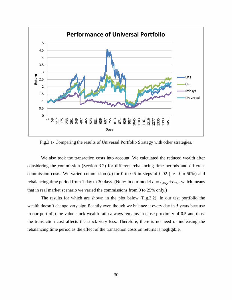
30
Fig.3.1- Comparing the results of Universal Portfolio Strategy with other strategies.
We also took the transaction costs into account. We calculated the reduced wealth after
considering the commission (Section 3.2) for different rebalancing time periods and different
commission costs. We varied commission for 0 to 0.5 in steps of 0.02 (i.e. 0 to 50%) and
rebalancing time period from 1 day to 30 days. (Note: In our model which means
that in real market scenario we varied the commissions from 0 to 25% only.)
The results for which are shown in the plot below (Fig.3.2). In our test portfolio the
wealth doesn’t change very significantly even though we balance it every day in 5 years because
in our portfolio the value stock wealth ratio always remains in close proximity of 0.5 and thus,
the transaction cost affects the stock very less. Therefore, there is no need of increasing the
rebalancing time period as the effect of the transaction costs on returns is negligible.
0
0.5
1
1.5
2
2.5
3
3.5
4
4.5
51
59
11
7
17
5
23
3
29
1
34
9
40
7
46
5
52
3
58
1
63
9
69
7
75
5
81
3
87
1
92
9
98
7
10
45
11
03
11
61
12
19
12
77
13
35
13
93
14
51
Re
turn
Days
Performance of Universal Portfolio
L&T
CRP
Infosys
Universal

31
Fig.3.2 – Effect of Transaction Cost on the returns of Universal Portfolio Theory
We expect the wealth to monotonically decrease as we increase our rebalancing period
but the plot above (Fig.3.2) doesn’t follow the trend. This is because the rebalancing done more
frequently takes care of all the abrupt changes and hence averages the risk. If the rebalancing is
not done frequently then we can lie either on the peak or on the low of the graph. But if we have
some extra information which can provide us accurate future market trends, then we can
rebalance our portfolio accordingly, in that case we can actually outperform CRP and Universal
both. A small discussion on this idea has been done in the next chapter.
Universal Portfolio Theory with commission is completely feasible and can provide far
better results as compared to other strategies. The best advantage of this strategy is that it
requires zero knowledge of market condition and is not susceptible to any abrupt changes in the
market. Although there is possibility of getting returns more than above strategy, but that
increases the risk. Overall, the above strategy is a very sound long term investment strategy with
far better returns for much lesser risk.
1.95
2
2.05
2.1
2.15
2.2
2.25
2.3
2.35
1 2 3 4 5 6 7 8 9 10 11 12 13 14 15 16 17 18 19 20 21 22 23 24 25 26 27 28 29 30
Re
turn
s
Rebalancing Period
Effect of Transaction Cost
c=0.14
c=0.16
c=0.18
c=0.20
c=0.22
c=0.24
c=0.26
c=0.28
c=0.30

32
CHAPTER 4
SIDE INFORMATION
Investors use various sources of side information to adjust their portfolios. We model this
side information as a finite valued variable made available at the start of each investment
period. The portfolio choice can then incorporate knowledge of for that period. Thus, the
formal domain of our market model is a sequence of pairs where, is the stock vector
for period and { } denotes the state of the side information at time .
The side information can arise in numerous ways. For example, sophisticated trading
strategies often develop signaling algorithms that indicate the nature of the investment
opportunity about to be faced. The signal would constitute the side information. Side information
could be world events, the behavior of a correlated market, or past information on previous stock
market data.
4.1 Side Information and the Doubling Rate
Theorem 4.1 Let be drawn i.i.d. from Let the log-optimal portfolio
corresponding to and let be the log-optimal portfolio corresponding to some other
density Then the increase in doubling rate by using instead of
is bounded by
( ) (
)
Note:
and
Proof: We have
∫ ∫
∫

33
∫
∫
⏞
∫
∫
⏞
where, (a) follows from Jensen’s inequality and (b) follows from the Kuhn- Tucker conditions
and the fact that is log optimal for .
Note: ∫
(also known as Kullback–Leibler divergence)
Theorem 4.2 The increase in doubling rate due to side information is bounded by
Proof: Given side information the log-optimal investor uses conditional log-optimal
portfolio for the conditional distribution . Hence, conditional on , we have,
from Theorem 4.1,
∫

34
Averaging this over possible values of we have
∫ ∫
∬
∬
Hence the increase in doubling rate is bounded above by the mutual information between the
side information and the stock market [10].
Above result is quite intuitive because mutual information can also be represented
as , where is the entropy. If Entropy is regarded as a
measure of uncertainty about a random variable, then is a measure of
what does not say about . This is "the amount of uncertainty remaining about after is
known", and thus the right side of the first of these equalities can be read as "the amount of
uncertainty in , minus the amount of uncertainty in which remains after is known", which is
equivalent to "the amount of uncertainty in which is removed by knowing ". This
corroborates the intuitive meaning of mutual information as the amount of information (that is,
reduction in uncertainty) that knowing either variable provides about the other. And we expect
the growth rate of our portfolio to be directly proportional to the reduction in uncertainty in
arose due to the knowledge of , which is proven by the above theorem.
4.2 State Constant Rebalanced Portfolios
The constant rebalanced portfolio is extended to the state constant rebalanced portfolio by
allowing the portfolio decisions to vary with the side information . A state constant rebalanced

35
portfolio specifies portfolios and uses portfolio at time when
the side information state takes on value { }. The choice of results in wealth
∏
on the stock sequence and side information . The collection of state-constant rebalanced
portfolios with states will be denoted by
For a sequence of stock vectors and side information states we can determine the
best state constant rebalanced portfolio as the one achieving the maximum wealth. We denote
this portfolio by where,
And the maximum is overall portfolio assignments Let
Denote the maximum wealth. Thus the best state constant rebalanced portfolio strategy uses
portfolio and achieves a wealth of [15].
The number of degrees of freedom in a state constant rebalanced portfolio will be useful
in characterizing the subsequent results. A state constant rebalanced portfolio for states and
stocks has degrees of freedom. degrees of freedom for each of the portfolios
which must be specified. The requirement that the entries sum to one gives each portfolio
vector degrees of freedom, rather than , where is the number of stocks.

36
4.3 Example explaining impact of Side Information
We now present a simple example illustrating impact of side information on constant rebalanced
portfolio [15].
Let , and let
(
)
(
)
be the sequence of stock market vectors. Note that the first component of the stock vector
at time is constantly equal to for . This first component represents a risk free
asset (or cash). On the other hand, the second stock is highly volatile, jumping up and down
by a factor of or
each investment day. A buy and hold strategy in stock results in
∏ ; a buy and hold of stock results in ∏ , when is even. Also, the
sequence has been maliciously chosen to perform contrary to naïve expectation. For example,
whenever stock has outperformed stock in past, it plunges by a factor of
.
Now consider the behavior of a constant rebalanced portfolio on this sequence.
Then, for even,
.
Setting the derivatives to , we find the maximum wealth is achieved by rebalancing each time to
,
resulting in wealth
√ ,
for even). Since (
) (
) , for , the wealth grows
exponentially to infinity.

37
Now consider side information with sates:
∏
∏
∏
∏
Thus indicates whether the running price of stock exceeds stock (cash) at time . The
sequences look like this:
(
)
(
)
Note that the simple calculation based on the past yields side information that gives prefect
investment information. An investor knowing would make perfect investment decisions,
and hence the best state constant rebalanced portfolio is
By investing in the best stock each time, the wealth gained by the best state constant rebalanced
portfolio
,

38
for even. Of course this is much greater than the result from constant rebalanced portfolio.
4.4 Universal portfolio with Side Information
Universal portfolio with side information is defined similar to universal portfolio by
using a fresh universal portfolio on each subsequence of corresponding to the
times at which the side information takes on a given value [15].
(
)
∫
∫
where, is the wealth obtained by the constant rebalanced portfolio along the
subsequence { }, and is given by
∏ and .
4.5 Implementation on real Stock Market
As we mentioned earlier, side information can be any information which indicates the
future trends in stock market. In our case we looked into 2 stocks (HDFC and Infosys) which are
listed on both NYSE and NSE. As there is a time lag between U.S. and India, we can make our
decision in NSE by looking into the performance of the stock in NYSE. We used the
performance of the stocks on NYSE as the side information and updated the portfolio in NSE
accordingly. The universal portfolio with side information surpasses the returns of the universal
portfolio without side information. Test period taken for this exercise is 2 years. The returns of
universal portfolio theory with and without side information are compared in the plot below
(Fig.4.1).

39
Fig.4.1 – Comparison of Universal Portfolio with and without Side Information
Strategy Returns (for Re.1)
Universal Portfolio without side information 1.70
Universal Portfolio with side information 2.12
Clearly, credible side information can give an edge to your portfolio but the challenge is to have
access to 100% credible side information, which is near to impossible in real life situation. Most
of the time, we have to speculate the future trends and develop it into side information which
may or may not go in our favor.
0
0.5
1
1.5
2
2.5
1
22
43
64
85
10
6
12
7
14
8
16
9
19
0
21
1
23
2
25
3
27
4
29
5
31
6
33
7
35
8
37
9
40
0
42
1
44
2
46
3
Re
turn
Days
Plot showing the effect of side information
Without Side Info
With Side Info

40
REFERENCES
[1] “Hidden Markov models and the Baum-Welch Algorithm”. IEEE Information theory
society newsletter, Dec 2003.
[2] B. Nobakht, C.E.J. Dippel, and B. Loni. “Stock market analysis and prediction using
hidden markov models”, unpublished.
[3] L.R. Rabiner. “A tutorial on hidden markov models and selected applications in speech
recognition.” Proceedings of the IEEE, pages 257–286, 1989.
[4] Rafiul Hassan and Baikunth Nath. “Stockmarket forecasting using hidden markov model:
A new approach”. IEEE Computer Society, 2005.
[5] Wikipedia. Hidden markov model. http://en.wikipedia.org/wiki/Hidden_Markov_model.
[6] L. R. Rabiner and B. H. Juang. “An introduction to hidden Markov models”. IEEE ASSP
Mag., June: 4-16, 1986.
[7] T. M. Cover, “Universal Portfolios," Mathematical Finance, Vol 1, No.1, 1-29, January
1991.
[8] T. M. Cover, “Log Optimal Portfolios," Chapter in “Gambling Research:Gambling and
Risk Taking," Seventh International Conference, Vol 4:Quantitative Analysis and
Gambling, ed. by W.E. Eadington, Reno,Nevada, 1987.
[9] T. M. Cover, “An Algorithm for Maximizing Expected Log Investment Return,” IEEE
Transactions on Information Theory, Vol. IT-30, No. 2, March 1984.
[10] T. Cover and J. Thomas, Elements of Information Theory, Wiley, New York, 2nd
edition,
2006.
[11] Harry Markowitz, “Portfolio selection”, Journal of Finance, vol. 7, no. 1, pp. 77–91,
1952.
[12] J Kelly, “A new interpretation of information rate”, IEEE Transactions on Information
Theory, vol. 2, no. 3, pp. 185–189, 1956.
[13] R. Bell and T. M. Cover, “Competitive optimality of logarithmic investment”,
Mathematics of Operations Research, vol. 5, no. 2, May 1980.
[14] T. Cover, “An algorithm for maximizing expected log investment return”, Information
Theory, IEEE Transactions on, vol. 30, no. 2, pp. 369 – 373, mar 1984.

41
[15] T. Cover and E. Ordentlich, “Universal portfolios with short sales and margin”, in
Information Theory, 1998. Proceedings. 1998 IEEE International Symposium on, aug
1998, p. 174.
[16] T.M. Cover and E. Ordentlich, “Universal portfolios with side information”,
Information Theory, IEEE Transactions on, vol. 42, no. 2, pp. 348 –363, mar 1996.
[17] T. Cover and D. Julian, “Performance of universal portfolios in the stock market”, in
Information Theory, 2000. Proceedings. IEEE International Symposium on, 2000, p. 232.