Embed Size (px)
Citation preview

Stormwater Knowledge, Attitude and Behaviors:
A 2005 Survey of North Carolina Residents
Chrystal Bartlett

Acknowledgements This survey was funded by a Section 319 Clean Water Act grant from the Environmental Protection Agency, administered by the N. C. Division of Water Quality. The instrument was developed by East Carolina University’s Center for Survey Research in collaboration with the N. C. Department of Environment & Natural Resources. Data collection and analysis were performed by ECU’s Center for Survey Research. The Division of Water Quality’s Nonpoint Source Planning and Permitting sections, The DENR Offices of Environmental Education and Public Affairs, Drs. Bill Hunt and Deanna Osmond, North Carolina State University and Samantha Foushee, Project Manager, ECU Center for Survey Research provided special assistance. DENR’s Creative Services department provided layout and composition.

Contents 1. Introduction 1 2. Literature Review 2 3. Method 8 4. Findings 9 5. Recommendations 19
Illustrations 1. Representation by County 9 2. Where Stormwater Goes 11 3. Stormwater Treatment by Gender 12 4. Grass Clippings Disposal to Storm Drains by Education 13 5. Monthly Fertilizers by Income 14 6. Soil Test by Age 14 7. Vehicle Wash Water Drains to Street or Driveway 15 8. Pet Waste Pickup by Gender 17
Maps 1. North Carolina Phase II Counties 19
Notes Appendix A A-1 Survey Instrument Appendix B B-1 Frequency Counts Appendix C C-1 Cross-Tabulations I. Water Quality C-1 II. Where Stormwater Goes C-15 III. Lawn Care C-21 IV. Vehicle Care C-37 V. Pet Waste C-51

North Carolina Stormwater Survey 2005
Abstract North Carolinians’ awareness, perceptions and behaviors related to polluted stormwater runoff in
North Carolina were measured using a 31-item phone survey administered in August and September
of 2005. Findings indicate a slight majority perceive overall water quality in local streams, lakes and
rivers as good and the greatest perceived water pollution threats are trash dumped into lakes and
rivers by recreational users and the waste water from manufacturing and sewer treatment plants.
Most respondents did not know that stormwater flows untreated to the closest stream, lake or river.
Behaviors affecting stormwater pollution were also explored. Although slightly less than half of
respondents fertilize their yards, most of them do not use a soil test to determine soil needs. Most
North Carolina residents leave grass clippings on their lawns, wash their own cars and have their oil
changed at commercial facilities. However, the majority of pet walkers do not dispose of pet waste
properly, and small groups report dumping used oil into storm drains or onto grassy areas as well as
over-applying fertilizer to their lawns.
Introduction
Stormwater runoff pollution, the dirty, untreated water resulting when rain or snow melt picks up
pollutants en route to area streams, rivers or lakes, has been cited as the greatest threat to water
quality in the United States. To address this problem, many states are administering the United
States Environmental Protection Agency’s “Phase II” federal stormwater program.
Under Phase II rules, entities that produce stormwater are regulated through permits. Permit holders
are required to employ best management practices that prevent or reduce polluted stormwater
runoff, conduct outreach and education, provide opportunities for public participation and perform
good housekeeping practices within their own operations. The program is an extension of the Phase
I National Pollution Discharge Elimination System implemented in 1990. North Carolina has issued
over 100 Phase II permits to counties and cities.
Gathering baseline measures of state residents’ knowledge of stormwater, their perceptions regarding
water quality and the behaviors that negatively impact stormwater runoff will improve future state
and local government outreach efforts. The benefits lay in knowing where to focus campaign
materials and how best to frame issues for different target audiences. Additionally, the baseline levels
provide a ruler by which the success of future campaigns can be assessed. Two additional, annual
surveys will be administered to gather this data. The survey output will increase campaign
effectiveness while providing valuable feedback on efficiency.
1

North Carolina Stormwater Survey 2005
Literature Review
Surveys measuring pre and post campaign effectiveness are an old tool, but given stormwater’s
relatively new focus, they have only recently been used in this area. As a result, few comparable
surveys are available for review. For this reason, the surveys used here should be considered in the
broadest comparative sense. Statistically speaking, no comparisons are possible given the variety of
instruments used, the times they were administered and the various vehicles used to deliver the
instruments. However, anecdotal and empirical data have value – not just in the findings themselves
but in the comparisons those findings make possible.
The majority of surveys were ‘snapshots” in that they were only designed to be administered a single
time. For this reason, trend analysis data were not widely available. All surveys gathered invaluable
data, however, in that they captured different audiences’ knowledge, perceptions and behaviors
regarding water quality and stormwater runoff. This holds true despite the varying degrees of
outreach done on polluted stormwater runoff in the communities that received surveys. North
Carolina’s residents have also been exposed to varying levels of stormwater outreach.
By gathering background knowledge on different states’ outreach efforts, some crude reverse
engineering efforts can also be made to determine the impact of specific outreach efforts. By
applying lessons learned in other locations, North Carolina can avoid financial pitfalls, capitalize on
others’ success and, it is hoped, create the most effective and efficient stormwater outreach campaign
possible for its regulated municipalities and state residents.
Threats to Water Quality
In South Carolina, a 2002 statewide phone survey showed residents perceived industry as a larger
threat to water quality than cities (USC, 2002, p. 4). A 2003 survey of Tennessee residents found
agriculture, automotive fluids and constructions runoff as the biggest perceived water quality threats
(Gant & Daugherty, 2003, p. 8). Tennesseeans perceived a variety of commercial/industrial and
individual activity as having negative impacts. Michigan’s 1993 study showed Wayne County
residents considered business and industry activity as having the greatest impact to local water quality
(Wayne County, 1994, p. 37). Conversely, a 1998 Colorado survey revealed almost one fifth of
residents do not consider automotive fluids – typically an individual waste product – as a water
quality threat (ZumBrunnen, 1998, p. 2). Only Maine’s 2004 survey of public employees showed an
emphasis on individual activity. Respondents cited malfunctioning septic systems, automotive fluids,
2

North Carolina Stormwater Survey 2005
litter and incorrect household hazardous waste disposal as major causes of water pollution (Hoppe,
2005, p. 14).
The tendency for individuals to hold business, industry and large public enterprise responsible for
water pollution is considered both a remnant of earlier outreach campaigns dating from over 20 years
ago and a common human tendency to blame negative events on external sources. Twenty years ago,
business, industry and large public facilities represented the largest water quality threats. Years of
regulation applied to point source water pollution dischargers, however, has substantially reduced the
contaminants these entities produce. Now, the EPA’s research shows individual behaviors that
create stormwater runoff represent the greatest threat to water quality.
Social psychologists have long noted that external impacts tend to be maximized over internal
decisions when associated with negative outcomes. This tendency, known as ‘self-serving bias,’ is the
tendency for humans to take credit for success but to blame external causes for failure (Bernstein et
al, Chapter 17, 2003). When applied to social marketing efforts, the concept may play a role in many
areas as diverse as weight loss (fast food), violent behaviors (media influence) and teen smoking
(advertising). The probability of this concept playing a role with regard to individual perceptions of
responsibility for stormwater is high. Regardless of the reason, the perceptions are reality in the minds
of those who believe them. Attempts must be made to educate residents about the role they play and
their responsibilities with regard to water quality.
Concern about water quality is widespread, but varies considerably in intensity. Few respondents in
any state perceive water quality as excellent or poor; most respondents head for the middle ground
and choose answers like ‘fair’ and ‘good.’ It appears that ratings are only partly associated with this
concern. Most of Maine’s public expresses concern about water quality, but feel their water is good
(Hoppe, 2004, p. 14). Most Tennesseeans also rate their water as good, but residents of cities are
more inclined to label its condition as “fair” (Gant & Daugherty, 2003, p. 1) and to express some
concern about the future. However, nearly half of Michigan’s Wayne County residents perceive their
local river’s water quality as poor (Wayne County Department of Environment, 1994, p. 36) due to
business and industrial waste (Ibid, p. 37).
Significant differences with regard to age, rural/suburban/urban location and income were noted in
some survey cross-tabulations. This suggests specific demographic groups, regardless of geographic
location, experience some common impacts that influence how they rate their water quality and the
degree of concern this rating evokes.
3

North Carolina Stormwater Survey 2005
Awareness of Stormwater
An awareness of stormwater’s contents, final destination and untreated status lays the foundation for
the individual thought processes required for behavior change. Stormwater is a relatively new topic
on the environmental outreach front and needs to ‘start from scratch’ in many respects.
Residents must be made aware of the link between their activities, the pollutants they generate and
the stormwater path before effective behavior change attempts can begin. Knowledge is commonly
accepted as a necessary but insufficient component for behavior change, because data – in and of
itself – does not motivate behavior change. The inverse is also true, however. Without knowledge,
the probability of success for behavior change is much lower.
Attempts to change behaviors without a foundation of knowledge can backfire. Castigating
individuals for actions they were not aware could damage water quality and can create resentment.
For this reason, establishing how much a population knows on the topic can guide outreach
professionals as to what type of campaign – action or awareness – is needed for a given target
audience. This approach also has the benefit of saving scarce funds.
Maine has done considerable public education on polluted stormwater and its impact on water
quality (Hoppe, 2005, p. 2). In a Maine survey of public employees, respondents’ top three choices
from a list of potential severe impacts to local water quality included two non-point and one point
source (pesticides, oil from cars and industrial discharges) (Hoppe, 2005, p. 14).
In a South Carolina survey of the state’s residents, more than half of the respondents considered
stormwater to have a great impact on water quality (University of South Carolina, 2002, p. 2). Only a
little more than a quarter of South Carolina residents know stormwater is not treated (Ibid, p. 3), so
their concerns may be attributed to other perceived sources of pollution. South Carolina residents
are hardly unique in this regard; less than 50 percent of Colorado’s state residents understand that
stormwater is not treated before entering local water bodies (ZumBrunnen, 1998, p. 2).
Individual Behaviors
Reported behaviors varied widely across the surveys reviewed, in part due to the variety of the
instruments themselves. While most surveys queried water quality perceptions and knowledge about
stormwater’s contents, destination and untreated status, few surveys measured individual behaviors.
4

North Carolina Stormwater Survey 2005
Maine surveyed its public employees about erosion by asking questions about buffers and about
using plants to cover bare spots in lawns. Erosion represents a serious problem to Maine waters, but
only 6 percent of the general population considered it a source of water pollution in 2004 (Hoppe,
2005, p. 2). Actually, the 6 percent represented progress that can directly be attributed to Maine’s
outreach efforts; no one cited erosion as a water quality threat in 1996!
Both South Carolina and Tennessee collected data on yard fertilizing, pet waste and grass clippings.
The two differed slightly with regard to automotive fluids; Tennessee considered them stand alone
items (Gant & Daugherty, 2003, p. 10), whereas South Carolina grouped them into the larger
household hazardous waste category (University of South Carolina, 2002, p. 15). In Tennessee, more
rural dwellers report changing their own oil than their urban counterparts. The overall average
reveals that a total of 20 percent of the population are considered “do-it-yourselfers” (Gant &
Daugherty, 2003, p. 5). In 2003, a survey of Salt Lake County, Utah residents also showed that a
quarter of residents changed their own oil, but 42 percent of them reported using commercial take-
back programs (Dan Jones & Associates, 2003, p. B7).
Car washing can represent a stormwater threat when soap, brake dust and road dirt wash off of
impervious surfaces, such as driveways, into streets, storm drains and the nearest water body.
Almost one-quarter of Salt Lake County, Utah residents wash their vehicles at home. Of this
number, over half (52 percent) reported they wash vehicles in their driveway (Ibid, p. B6). In
Vermont’s Chittenden County, where most residents wash their own vehicles, 68 percent reported
they routinely wash vehicles in the driveway (Lake Champlain Committee, 2004, p. 2). Lower
numbers appeared in Tennessee where only a quarter of car-washing residents reported washing
vehicles in their driveways (Gant & Daugherty, 2003, p. 4).
Most surveys revealed pet waste pickup to be a problem; few respondents reported proper disposal.
Close to one third of South Carolina’s dog walkers reported that they rarely or never pick up dog
waste (University of South Carolina, 2002, p. 23). Further analysis shows this state’s females are
more likely than males to properly dispose of pet waste (Ibid). Half of Tennesseans see pet waste as a
source of water pollution (Gant & Daugherty, 2003, p. 8), but no data was gathered on how residents
handle this waste product. In Salt Lake County, 41 percent of residents own pets, but few bag pet
waste deposited in public places (as opposed to their own yards) for disposal (Jones & Associates,
2003, p. B7). Vermont’s survey of Chittenden County residents showed that most residents don’t
dispose of pet waste regardless of whether the waste was deposited at home or on walks (Lake
Champlain Committee, 2004, p. 2).
5

North Carolina Stormwater Survey 2005
When over used, applied at the wrong time or in the wrong conditions, lawn fertilizers pose the
threat of phosphorus and nitrogen runoff. Because herbicides and pesticides are often combined
with fertilizers, the combined products often travel together in polluted runoff from yards and
negatively impact both water and the wildlife within it.
One might assume that people who do not test their soil would be more likely to apply too much
fertilizer. This is not always the case, per a survey performed in North Carolina, but the “low rate of
soil testing by homeowners in all communities demonstrates the need to stress soil testing, both to
individuals as well as lawn care companies” (Osmond and Hardy, 2002, p. 572). Fertilizer mistakenly
applied to impervious surfaces poses the greatest threat because it runs off in greater quantities.
A third of South Carolina residents fertilize once per year, with rural residents showing the lowest
frequency (South Carolina Department of Health and Environmental Control, 2002, p. 8). Less than
a third consulted their local cooperative extension for soil tests, although females reported contacting
the local extension service more frequently than males. A full 60 percent of Tennessee residents use
fertilizer regularly, with 25 percent doing so four times a year (Gant & Daugherty, 2003, p. 4). Only
25 percent of those who report using fertilizer also used soil tests (Ibid, p. 3); cross-tabulations
revealed residents with higher incomes and education levels tested their soil more than other groups
(Ibid, p. 4). In Salt Lake County, Utah, close to half (49 percent) of residents report that they fertilize
regularly (Dan Jones & Associates, 2003, p. B6), although no data were collected on soil testing.
Minnesota residents of the Tanners Lake Watershed report a fertilization rate of 71 percent (Ramsey-
Washington Metro Watershed District, 2002, p. 11), but no data on soil testing were collected.
Because yard waste can introduce excess nitrogen and phosphorus to water bodies via grass clippings
and leaves, disposal practices are an important behavior to track. Knowing the percentage of “do-it-
yourselfers” versus those who have their yards cared for by commercial enterprise can direct
outreach efforts to the most efficient audience: the general public or trade professionals. Audience
choice is heavily associated with media choice, so the same data can inform dissemination decisions.
In Salt Lake County, Utah, three quarters of county residents reported they mow their own grass, but
no data were collected on clipping disposal (Dan Jones & Associates, 2003, p. B6). In South
Carolina, 6 percent of residents dispose of their grass clippings in ditches and a small but troubling
one percent burn clippings in ditches (S. C. Department of Health and Environmental Control, 2002,
p. 12). Tennessee’s survey revealed hardly any residents report disposing of lawn clippings in storm
6

North Carolina Stormwater Survey 2005
drains (Gant & Daugherty, 2003, p. 2, and in a survey of Minnesota’s Tanners Lake Watershed, the
majority (63 percent) of yard mowers reported they left grass clippings on their lawn (Ramsey-
Washington Metro Watershed District, 2002, p. 7).
Overall, the behavior findings reveal wide national disparities with regard to activities that impact
stormwater. Many factors, including educational inputs, could be a factor in these results. The
literature reviewed here shows rural or urban resident status appears to play a role in oil changing and
pet walking behavior. Rural residents are less likely to walk dogs, wash vehicles on hardened surfaces
and fertilize their yards, but some surveys found they are more likely to change their own oil. Urban
dwellers have access to yard waste pickup, but few live with ditches in their yards. Urbanites are,
however, more inclined to wash vehicles on driveways. Gender also appears to play a role. More
women than men pick up pet waste for proper disposal. Some surveys show women are also more
likely to use a soil test before applying fertilizer.
Compared to the other behaviors that introduce stormwater pollutants, improper motor oil disposal
appears to occur rarely. This may be due to the large number reporting use of commercial oil change
facilities rather than any outreach efforts. Although their numbers are small, home oil changers who
report improper disposal still pose a threat. In North Carolina’s survey, some questions exist about
the reliability of the data – primarily due to the small numbers of respondents reporting the activity.
Despite the low numbers, outreach efforts should continue due to the damage even a small quantity
of waste oil can have on water quality.
One other question exists with regard to self-report data collected on this or any other negatively
perceived behavior. Social psychologists have observed that these behaviors (e.g. littering, spanking
children, drinking to excess, dumping used motor oil) are commonly under reported. There are
many reasons for this behavior, but handling the end result can be problematic. Some researchers
simply use the numbers reported; others may adjust them slightly up or down, still others use the
numbers, but point out where the high risk of under reporting exists. The latter approach is
employed with this survey instrument’s finding.
While the body of stormwater survey literature is small, it holds great promise for the future. Many
instruments were inspired by the Environmental Protection Agency’s requirements for regulated
entities to measure outreach programs. While surveys are not required, their increasing use bodes
well for the field. The need for comparison data will no doubt increase homogeneity across
7

North Carolina Stormwater Survey 2005
instruments, as has been the case with many other research fields. The desire to compare data is
often a strong enough motivation to inspire researchers to create the very datasets currently missing.
Method
Instrument
A 31-item survey instrument (see Appendix A) was created in partnership with East Carolina
University’s Center for Survey Research. It was designed to measure awareness, perceptions and
behaviors related to water quality and polluted stormwater runoff in North Carolina. The same
instrument gathered respondent data on gender, age, income, education and ethnicity. Respondents’
telephone numbers were coded as urban, suburban or rural by the company who provided the
sample of phone numbers.
Participants
Respondents for this survey were selected from a random sample of households with telephones in
the state using random digit dialing. The sample of 11,200 telephone numbers was purchased from a
reputable survey sampling company.
Procedure
Data for the survey were collected between August 2005 and September 2005. Over 11,000 calls
were placed to capture 1,000 completed surveys. With a sample size of 1,000, the confidence level is
95 percent and the confidence interval is ± 3.1. Nine interviewers that were trained and employed by
ECU’s Center for Survey Research administered the survey. Interviewers used a computerized
telephone assisted interview (CATI) software system.
Methodology
The data were compiled and analyzed by the ECU Center for Survey Research. After validity and
reliability were established, data were analyzed using frequencies (see Appendix B) and cross-
tabulations (see Appendix C). For all statistical findings, significance levels were set at p ≤ 0.05.
A chi-square goodness of fit test showed a significant difference between the number of males and
females in the sample compared to the expected number, which was based on 2000 Census data for
the state. A significant difference was also noted between the sample and the population with regard
8

North Carolina Stormwater Survey 2005
to the race categories of African-American, Asian, White, Hispanic and Other. Data on age,
household income and education levels could not be evaluated using this measure due to
overwhelming differences in the categorization of the data in the survey instrument when compared
to census data categories.
Cross-tabulations were performed on the survey questions that measured respondents’ perceptions
of overall water quality in area lakes, streams and rivers using all demographic data points: dwelling
area, gender, race, education level, age, household income and retirement status.
Some responses had abnormal amounts of missing data. Confidence intervals were calculated for
each of these questions. Each yielded a confidence level of 95 percent with all of the intervals
calculated at less than ± 4. Even with the missing data, the survey was still statistically sound.
The data were transformed for the water quality question in an effort to create fewer groups within
the data. For example, ‘excellent’ and ‘good’ responses were combined to create the value
‘Good/Excellent’ and ‘poor’ and ‘fair’ responses were combined to create the value ‘Poor/Fair.’
‘Don’t know’ responses kept their original label and value.
Other survey questions were cross-tabulated with selected demographic data sets. Some of these
analyses revealed statistically significant associations.
Findings
Demographic Data The most represented counties in
this survey are also North
Carolina’s most populous: Wake
(9.4 percent), Mecklenburg (4.8
percent), Guilford (4.4 percent)
and Cumberland (3.5 percent).
Urban respondents made up 26.7
percent of the total, suburban respondents comprised 38.7 percent and 34.6 percent of respondents
lived in rural areas. respectively.
9

North Carolina Stormwater Survey 2005
The race categories reported by respondents, from largest to smallest, were: White (55.4), Black or
African-American (17.1), Hispanic (9), Other (7.5), Asian (3.8), Don’t Know (6.1) and Refused to
Answer (1 percent).
Respondents reported age categories, from youngest to oldest, fell into the following percentage
groupings: 18-24 years (10.8), 25-34 years (8.1), 35-44 years (31.3), 45-54 years (17.7), 55-64 years
(13.7), 55-64 years (13.7), over 65 years (7) and Refused to Answer (1.0).
The household incomes reported showed that 12.1 percent of respondents made less than $12,000
annually. The other income categories, from lowest to highest, were: 12K-25K (13.9 percent); 25K-
35K (12.3 percent); 35K-50K (13.9 percent); 50K - 75K (14.6 percent) and 75K-100K (7.9 percent).
Only 7.2 percent of respondents reported earning more than 100K and 15 percent responded that
they did not know their income. A total of 3.2 percent of respondents refused to answer.
Respondents’ education levels were divided into the following categories, with percentages following:
less than high school (4.2), some high school (23.5), high school graduate (10.1), some vocational or
technical school (6.5), graduated from vocational or technical school (15.1), some college (5.9), two-
year college graduate (15.4), four-year college graduate (7.9), and post-graduate (7.9).
Water Quality
More North Carolinians perceive the water quality of streams, lakes and rivers as Good (42.4
percent) than Fair (39.4 percent), with the minority (13.2 percent) rating water quality as Excellent.
Urban dwellers were more likely to view water quality positively than their rural and suburban
counterparts. With regard to gender, slightly more men than women rated water quality as
“fair/poor” rather than “good/excellent.”
Education played a slight but irregular role with regard to water quality perceptions. Quality
perceptions were slightly more positive among those reporting postgraduate, vocational/technical
and high school backgrounds.
Only the youngest respondents, those aged 18-24 years old, perceived water quality positively, but
only by a slight margin.
Income did not play a significant role, but those in the highest income bracket viewed water quality
most positively by a slight (0.7 percent) margin.
10

North Carolina Stormwater Survey 2005
None of these findings were considered statistically significant, with the exception of retirees.
Compared to non-retired residents, only retirees are significantly more inclined to rate streams, lakes
and rivers as “good/excellent.” This was the only demographic cross-tabulation with regard to water
quality that registered as statistically significant.
Stormwater
Knowing where stormwater goes and what it contains forms the building blocks for behavior
change. Unless residents know that their behaviors directly impact water quality, they have little
reason to change their behaviors.
Unfortunately, many surveys show a common misperception exists: many people believe stormwater
is treated. They may not be sure where it is treated or how it is treated, but they feel sure that some
treatment is being administered. This misperception persists even in states that do not co-mingle
stormwater and sewer effluvia, like North Carolina.
Only over a third of North Carolina residents (37.6 percent) know that stormwater flows to the
closest stream, lake or river and 13.2 percent believe it flows to drainage ponds, which may be a
stormwater best management practice.
However, 28.7 percent believe stormwater
receives treatment at a special plant or the
sewer treatment plant. Fields and yards was
the destination chosen by 9.8 percent of
respondents and 10.7 percent refused to
answer the question.
When cross tabulations were performed using
demographic attributes, both age and gender
significantly impacted responses. If you
combine the answer categories, you can
separate the choices into two categories: ‘treated” and “untreated.” Respondents who chose “the
city’s regular sewer plant” or “a separate special sewer treatment plant” answers believe stormwater is
treated. Those choosing one of three possible answers: “nearby fields and yards,” drainage pond”
and “closest stream, river or lake” were placed into the ‘untreated category.
11

North Carolina Stormwater Survey 2005
Using these groupings, the ‘treated’
category is comprised of 9 percent of men
and 20 percent of women. In the
‘untreated’ category, women made up 34
percent of the total and men composed
30 percent.
Results for the single response “closest
river, stream or lake” fell into the
following gender categories: 19 percent
male and 18 percent female.
When classified by age, respondents choosing the “closest river, stream or lake” answer fell in the
following rank order, with percentages following: 55-64 years (42 percent), 35-44 years old (41
percent), over 65 (39 percent), 25-34 year olds (35 percent), 18-24 year olds (34 percent) and 45-54
year olds (32 percent).
When responses were grouped into the previously described “treated” and “untreated” categories,
the following age rankings, from largest to smallest percentage, were found in the “treated” category:
18-24 year olds (36 percent), 45-54 year olds (33 percent), 25-34 year olds (32 percent), 35-44 year
olds (31 percent), 55-64 year olds (30 percent) and respondents 65 years or more (18 percent).
Age rankings in the “untreated” category, from largest to smallest percentage were: 55-64 year olds
(63 percent), 18-24 year olds (62 percent) and – in a tie for fourth position - 25-34 year olds and 35-
44 year olds (58 percent) and - in a tie for fourth position - 58 percent by the 25-34 and 35-44 year
age groups. The 45-54 year olds took the final rank position with 58 percent of respondents
choosing this answer.
Lawn Care
Few practices have the potential to impact stormwater to the degree of lawn care. If grass were
harvested as a crop, it would represent one of the United States’ largest commodities (USDA, 1992).
Fertilizers, pesticides and herbicides can and do wash into creeks and streams, but the degree of
impact they pose is still being studied (Schueler, T., 1995a, p. 35). Yard waste, like grass clippings and
fallen leaves left in the street, can also wash into water bodies via storm drains where they introduce
12

North Carolina Stormwater Survey 2005
excess nitrogen and phosphorus. When the algae blooms they can induce die off, they use so much
of the water’s available oxygen fish kills can result. Since pesticides and herbicides are often mixed
into fertilizers, these chemicals often accompany fertilizer in polluted stormwater runoff. Their
presence poses additional risks to the flora and fauna that live in and around the receiving waters.
Most of North Carolina’s survey respondents (96 percent) reported having a yard that they personally
mow. When these same respondents were asked how they disposed of grass clippings, the majority
(53.7 percent) reported leaving the clippings in the yard. This practice, known as grasscycling, reduces
the need for fertilizer applications by returning nitrogen to lawns. It also protects local waters.
Mulching and composting yard waste, another water protective behavior, was the option chosen by
16.4 percent of respondents, but the second largest group of respondents (26 percent) stated that
they collect grass clippings for disposal in the garbage. A small but troubling 1.5 percent report
raking or blowing grass clippings into storm drains.
Grass clipping disposal methods
appear to be significantly influenced
by education level, but not in the
intuitive sense. One might assume
that higher levels of education are
positively associated with more
environmentally protective practices
like grasscycling and composting.
However, the only categories that
did not report any storm drain
disposal of grass clippings had either
attended or graduated from a
vocational or technical program or held a post graduate degree. All other educational levels reported
small levels of storm drain disposal with the highest numbers appearing in high school graduates and
those with some college.
Because North Carolinians live in three distinct physiographic areas - the coast, the Piedmont and the
mountains – planting, fertilizing and growing times vary statewide. Less than half, (39.1 percent), of
state residents claim that they fertilize their own lawns. Of that group, most respondents (58
percent) report fertilizing their lawns once a year or less. The next largest group (36 percent)
13

North Carolina Stormwater Survey 2005
reported that they fertilized their yards two to three times per year. A troubling 5 percent reported
applying fertilizer monthly, although no grass requires this much fertilizer.
Annual household income is significantly
associated with the frequency of fertilizer
applications. Survey results showed that
those earning more than $100,000 per year
report applying fertilizer monthly more than
any other income level. The second group,
made up of respondents who report
applying fertilizer two to three times
annually, were most likely to earn (in rank
order) $50,000 to $70,000; over $100,000;
and $35,000 to $50,000.
The age of respondents was also significantly associated with fertilizer applications. Here, we find
the 35-45 year olds (12 percent) are more likely than any other age group to fertilize their lawns
monthly. The youngest group, 18-24 year olds, was most likely to apply fertilizer “two or three times
a year” with an overwhelming 85 percent choosing this response. The next largest groups were 35-
44 year olds (63 percent), 45 to 54 year olds (43 percent) and those 65 years or older (35 percent).
Respondents aged 55-64 years were most likely to report applying fertilizer once per year (69
percent). They are followed in rank order by those aged 25-34 (64 percent), 65 years or older (59
percent) and 45-54 year olds (54 percent).
The best way to learn a yard’s fertilizer needs is
to conduct a free soil test available from the
state’s Department of Agriculture & Consumer
Services. If respondents indicated they fertilized
their own yard, they were also asked if anyone
ever tested the soil. The majority (54 percent)
responded that they did not use soil tests, but 44
percent of respondents did report testing their
soil to determine fertilizer needs.
14

North Carolina Stormwater Survey 2005
Soil testing for fertilizer levels was also significantly related to age. The respondents mostly likely to
test their soil were aged 35-44 years, followed by those 45-54 years of age, and the third place was
tied between 18-24 year olds and 55-64 year olds. Conversely, those least likely to test soil were over
65 years of age, followed distantly by the 25-34 year olds.
Vehicle Care
While a host of possible questions exist about vehicle care, this survey chose to explore two activities:
washing and oil changing. When vehicles are washed at home, the soapy wash water and the brake
dust and other road dirt it carries usually go to one of two places: a grassy area that absorbs water and
its constituents or a driveway that serves as a connector for the gutter and storm drain system.
Vehicles washed at commercial facilities do not present the same threat because state regulations
require these facilities to use oil/grit separators.
In this survey, three quarters of respondents stated that they had a vehicle. Of that group, 40 percent
stated that they washed their vehicles at home. The majority (56 percent) washed vehicles in the
driveway, but 41 percent let soapy wash water flow into grass, dirt or gravel.
Where respondents live significantly affects the
destination of soapy vehicle wash water. Half
of urban dwellers reported letting soapy water
drain into “the street or a driveway,” whereas 40
percent of suburban dwellers and 29 percent of
rural dwellers report the same practice. The
inverse was also true: more rural dwellers (66
percent) let soapy car wash water drain into “the
grass, dirt or gravel” than suburban (52 percent)
or urban (47 percent) dwellers.
The majority of respondents (75 percent) who reported they owned a vehicle were asked if they
changed their own oil. Of that group, less than a fifth (16.7 percent) reported doing so. The
overwhelming majority (76.9 percent) reported using commercial oil change facilities.
Home oil changers dispose of oil in a variety of ways; no single disposal practice monopolized the
responses. The most frequent answer (32.2 percent) was to place used oil with other garbage for
15

North Carolina Stormwater Survey 2005
disposal. Slightly more than one fifth report taking oil to a recycling facility. Two especially
troubling findings cropped up next: 22 percent of respondents dump oil onto a designated part of
their lawn and 20.6 percent pour used oil down storm drains. Although these numbers represent a
fraction of North Carolina residents, the finding is troubling: one quart of oil can contaminate one
million gallons of drinking water.
Race does appear to play a significant role in oil disposal practices, but respondent numbers – while
representative – were quite low in some groups. For this reason, the following data should not be
viewed as conclusively as the other findings presented here.
It is difficult to determine which factors are at play. Without knowing how long respondents have
lived in the United States, much less North Carolina, it is impossible to tell if their disposal practices
are a vestige of their country of origin or due to a lack of information on the topic. Residents may
also be confused as to proper waste oil disposal practices. Not long ago, many municipalities and
businesses all over the world viewed spraying waste oil onto dusty roads as an excellent dust
suppression method.
Survey respondents’ waste oil disposal choices in the survey were: recycling, placing with garbage,
placing in a designated lawn area, dumping down a storm drain or “other.” Asian respondents
reported storm drain dumping in higher percentages than any other group, but a greater number of
white respondents reported that they placed used oil in a designated lawn area. Every group but
Asians cited recycling as their leading disposal practice. After recycling, the most frequently cited
disposal method was “placing with garbage” followed by disposal in a “designated lawn area.” A
larger percentage of white respondents (8 percent) chose the “designated lawn area” response. The
next largest group reporting this behavior (4 percent) chose “don’t know” as their racial
classification.
Although it may take longer to reach the stream, used oil disposed on lawn areas can negatively
impact surface water supplies through runoff. At a minimum, the local groundwater supplies can be
contaminated as the waste oil leaches its way through the soil.
Pet Waste
Just like poorly maintained septic tanks, pet waste represents a microbial threat to water quality.
Typically, one assumes that dogs are the pets to be walked, but that may not always be the case.
16

North Carolina Stormwater Survey 2005
Research actually shows that cat and raccoon waste pose larger microbial threats (Schueler, 2000, p.
82), but until these species are routinely guided on walks over impervious surfaces – especially those
near or surrounding water bodies – the focus remains on man’s best friend.
Respondents who claim they walk their pets were asked how often they picked up their pet’s waste.
A significant relationship exists between reported pet waste disposal and dwelling area. As expected,
urban and suburban dwellers reported more pet walking than their rural counterparts. Respondents
claiming that they ‘rarely” or ‘never’ picked up pet waste comprise 47 percent of urban pet walkers,
49 percent of suburban pet walkers and 59 percent of rural pet walkers. Those reporting they
“always” or “often” picked up pet waste comprised 35 percent of urban dwellers, 34 percent of
suburban dwellers and 27 percent of rural pet walkers.
Respondent age was significantly associated with pet waste pickup. North Carolina’s youngest (18-
24) and oldest residents (65 years and older) are most likely to report they “always” or “often” pick
up pest waste. Two age groups tied for the ‘least likely to pick up pet waste’ category: 35-44 and 45-
54 year olds. The next largest age groups in the ‘least likely’ category were 25-34 year olds and 55-64
year olds.
Gender also plays a significant role
with regard to pet waste pickup.
Women are more likely to report they
“always” or “often” pick up pet waste
(35 percent) than men (28 percent).
Conversely, men were more likely to
report they ‘rarely’ or ‘never’ picked
up pet waste (57 percent) compared
to women (46 percent). Respondents
choosing the ‘sometimes’ answer
were more evenly split along gender lines; slightly fewer females (11 percent) than males (13 percent)
chose this answer.
Discussion The study’s findings represent a mix of intuitive and counterintuitive results, although no formal
hypotheses were made. Assumptions that greater levels of education would be associated with more
17

North Carolina Stormwater Survey 2005
stormwater knowledge were proven to be false. Respondents’ knowledge levels and water protective
behaviors did not rise in association with formal education levels. Another assumption, that soil
testers would apply less fertilizer, was not proven by the findings.
Some soil testers reported applying fertilizer monthly, although no lawns require monthly
applications for good health. It was also assumed that higher income households would be less likely
to self-apply fertilizer and instead use a lawn care service. However, many of North Carolina’s most
well-to-do homes report performing this service themselves.
It was also assumed that rural dwellers would be more inclined to change their vehicle’s oil, but this
was not the case. “Do it yourselfers” were evenly distributed throughout all dwelling categories.
Some assumptions were borne out by the survey’s results. As with other surveys, women were most
likely to dispose of pet waste properly. Urban and suburban dwellers reported higher levels of pet
waste pickup than their rural counterparts. Urban dwellers were found to be more likely to wash
their cars on impervious surfaces, such as streets and driveways, than rural dwellers. As assumed,
rural dwellers were found to be most likely to have soapy water drain into a pervious area such as
grass or gravel. Income, which was assumed to influence fertilizer application (albeit through
professional services), was indeed found to play a role in North Carolina, although it was not the role
expected. Instead of hiring services, North Carolina’s wealthy respondents reported that they apply
fertilizer themselves. They also reported that they fertilize more frequently than any other group.
Although no assumptions were made with regard to water quality, the findings were surprising.
North Carolina’s ranking as a high retirement destination state inspired this demographic question,
but it was only associated with one perception. Only retirees rated water quality as “good” or
“excellent.” There were no correlations between water quality perception with regard to race, gender,
income, education or dwelling area.
18

North Carolina Stormwater Survey 2005
Recommendations Survey findings can be used to strategize the mandated outreach and education to be conducted by
Phase II designated communities. Demographic groupings are essential for efficiency when targeting
media message content. It can also guide the media chosen to deliver those messages.
Logic demands that humans need motivation to change behaviors. With less than 50 percent of the
population aware stormwater is not treated before entering local water bodies, awareness of this fact
must be emphasized before, or in conjunction with, messages requesting behavior change. Residents
must first understand the link between their behaviors and water quality before they can reasonably
be expected to make voluntary changes in their daily activities.
In this survey, urban audiences were
not shown to be any more aware of this
link than anyone else surveyed. These
findings are surprising because urban
audiences were most likely to live in
areas where EPA’s Phase I program
was already in progress. The program,
which began in 1990, addressed sources of stormwater runoff that had the greatest potential to
negatively impact water quality. As with the Phase II program, permittees are required to provide
education and outreach to their communities. Census-defined ‘urban’ areas created the starting point
for selection of Phase I communities, but other qualifications in addition to the census definition
were applied in the selection process. For this reason, comparisons of Phase I communities and
census-designated ‘urban’ area are problematic because the two are not ‘like’ items. Rather, Phase I
communities comprise a subset of ‘urban’ communities.
Phase II communities also use census designations as their starting point, but as with Phase I, other
requirements play a role in the designation process. Permit holders include communities with
medium and large municipal separate storm sewer systems (MS4s) with populations of 100,000 or
more and companies that fall into one of eleven categories of industrial activity, including
construction activity that disturbs five or more acres of land. Proximity to sensitive waters and
growth rates also play a role in the selection process.
19

North Carolina Stormwater Survey 2005
Because the bulk of urban resident respondents live in Phase I communities, one might easily assume
they would demonstrate higher levels of stormwater knowledge. However, given the fact that they
do not demonstrate significantly higher levels of knowledge, the need for basic information
campaigns in these areas still exists. Information campaigns conducted by both Phase I and Phase II
communities should continue to feature basic information messages in tandem with messages
encouraging water-protective behaviors.
Basic information messages should also be targeted toward women because this group knows less
about stormwater’s destination and treatment status than their male counterparts. Media buys and
participation in events that focus on women are efficient ways to reach this group.
Targeting messages by age group will also yield results, although the demographic breakdowns are
not as discrete as was hoped. The groups with the lowest awareness of stormwater’s untreated status
are not linear; instead they jump from age group to age group. With more 18 - 24 year olds than any
other age group thinking stormwater is treated, we need to devise and place messages that attract this
demographic. Youth messages can be clearly defined, but what of the next group most in need of
this information? They are 45-54 year olds whose media and message preferences do not overlap to a
great degree (Paul, March 2003). The third group, 25-34 year olds, do share media choices and
message preference with the first group (18-24 year olds), so messages that appeal to the first and
third ranked groups could be created and distributed together for cost efficiencies.
With regard to lawn care, mass media messages should be used. With so many respondents mowing
their own lawns, including a business-to-business campaign would be comprehensive, but if cost
efficiencies are an issue, the single largest group is consumers. The majority of lawn mowers in
North Carolina are “do-it-yourselfers,” so point of purchase, broadcast and direct mail would reach
this group most effectively.
Because education levels were not linearly associated with grass clipping disposal, reaching this
audience through educational venues would be problematic. Residents who graduated or attended a
vocational or technical school used the most protective practices, followed by those with post-
graduate degrees. Some work may be done through educational institutions, but this is likely to yield
lower outcomes given the wide distribution of the audience to be targeted.
Annual household income levels were positively associated with excessive fertilizer application, so
messages should be placed in media targeted to higher incomes. Broadcast media can be used in this
20

North Carolina Stormwater Survey 2005
fashion, but print media is a more efficient way to reach those with high incomes. Because this
audience values appearance (Schueler, 2000, p. 673), care should be taken to stress that fewer
fertilizer applications could yield the same aesthetic outcomes they value so highly.
Soil testing was significantly associated with age, but the absence of a linear trend presents a
challenge. Those aged 65 years or over were least likely to report using a soil test, followed by the
25-34 year olds, who were followed by 55-65 year old respondents. Audiences over 65 respond well
to economic benefit messages due to the high number on fixed incomes, but this rhetoric is not as
effective with those in the 55-65 year old age group, who respond better to lifestyle motivations. The
25-34 year old demographic is less likely to respond to economic and lifestyle messages, but more
likely to respond to environmental benefits. Clearly, a mix of message appeals is needed to reach
these different groups effectively.
Distribution also represents an efficiency challenge. Media choice preferences are most likely to be
shared by similar age groups, so venues preferred by 55-65 year olds are more likely to cross over
with the group aged 65 years or older. However, the messages most likely to be effective differ
between these two groups. It may be that point of purchase appeals at retail fertilizer outlets work
best because all groups purchase this product. This distribution method does not allow for custom
messages for each age group, but does offer the advantage of being able to reach more of this
audience than any other outlet.
Findings on vehicle care did yield some useful targeting data. Urban and suburban dwellers are most
likely to wash cars on impervious surfaces, so efforts should be made to focus behavior change
messages in these areas. Because direct mail and outdoor advertising (e.g., billboards, busses, bus
shelters and kiosks) can be geographically targeted more easily than broadcast media (with the
exception of cable), messages using these media will be most likely to reach their targets.
The advent of the $20 oil change decreased the number of do-it-yourself oil changers nationally and
North Carolina is no exception. With only 16.7 percent of respondents changing their own oil, one
might be tempted to focus on other, more prevalent behaviors. However, the incredible impact of
dumping even small quantities of used motor oil in local streams, creeks and rivers makes this
message too important to neglect.
The fact that race plays a role in oil disposal poses additional challenges. North Carolina’s Asian
community reports the highest numbers of oil dumping in storm drains; those most likely to dispose
21

North Carolina Stormwater Survey 2005
of oil on lawns are white. As the smaller group, targeting the Asian community is less problematic
from a marketing standpoint, but the potential for complications surrounding racial targeting are so
high that any benefits accrued may diminish in comparison. Targeting the self-described ‘white’
community represents an inverse challenge. They comprise the largest racial group in North Carolina,
which suggest mass media as the best distribution point. However, the low numbers reporting this
activity mean the audience will be so scattered that the cost may be wasteful given the return.
Pet waste messages pose a unique set of problems regardless of target. Because discussion of waste
products is widely considered taboo in popular culture, careful message preparation is key to avoid
losing the message in the provocative topic.
Targeting along geographic lines is the logical step given the findings. Just like their car-washing
cohorts, urban and suburban residents are most likely to be surrounded by impervious surfaces. Pet
walkers in these areas are also more likely to congregate in smaller areas. Even though urban and
suburban audiences are more likely than their rural counterparts to pick up pet waste, they do so in
low enough numbers that this message needs to be focused in this geographic area.
Rural dwellers are least likely to walk their pets and are also least likely to dispose of pet waste.
However, this group is surrounded by more pervious surfaces that absorb the waste and they are
more widely scattered geographically. As a result, they may present less of a water quality threat. For
these reasons, messages about pet waste should be broadly distributed, but priority should be given
to urban and suburban areas. A broadcast and outdoor media campaign augmented by point of
purchase displays at pet care retail outlets and veterinarian’s offices could deliver these qualities.
Should a list be available, piggybacking on direct mail to dog owners from their veterinarians would
be most effective and efficient.
The age of respondents was associated with pet waste disposal. North Carolina’s youngest (18-24)
and oldest (65 years +) pick up pet waste the most, so messages should be focused at the ages in
between. Respondents aged 35-44 and 45-54 are least likely to pick up pet waste and share many of
the same media preferences with regard to both outlet and message appeals. Here, a single campaign
can be created for this large audience and distributed using mass media.
In addition to age and dwelling location, gender significantly influences pet disposal patterns. Just as
women need more education about stormwater destination and pollutant contents, men need
education on the negative impact of improperly disposed pet waste. How the messages are framed
22

North Carolina Stormwater Survey 2005
for these different groups is key. Women have been shown to respond more positively to health
messages, but men are more inclined to respond to lifestyle messages. Appeals based on pet waste’s
impact on recreation, fishing and outdoor enjoyment may be most effective with male audiences.
Distributing these messages through lifestyle oriented media such as point of purchase displays at
retail sporting and recreation outlets may prove effective. Relationships should be created to allow
messages to be distributed where these activities occur – at public lakes, rivers and other outdoor
recreational areas.
In summary, this survey represents a road map of sorts for North Carolina’s social marketing efforts
with regard to stormwater. Although time limitations for a phone survey precluded asking every
question desired, the questions used provide a wealth of material with regard to the messages needed
and their most effective targets.
Two follow up surveys are planned for the years 2006 and 2007. These surveys will gather trend data
on the questions asked in the 2005 instrument. They will also gather data on awareness and retention
of social marketing efforts conducted in the interims between surveys. These data will allow North
Carolina’s stormwater social marketers to refine their outreach efforts in two major ways. Marketers
can concentrate efforts where and to whom they are most needed. They can see where campaigns
have produced positive changes and adopt the programs used in those areas. They will also be better
equipped to measure message efficiency and effectiveness within specific demographic groups.
Again, the strategy is to identify successful programs and administer them where needed.
The social marketing strategies recommended here did not consider cost to a great degree. As such,
they represent an “ideal world” scenario. While such a world does not exist, the recommendations
provide a framework for planning, fundraising and future cooperative efforts between government,
business and community or interest groups focused on the same issues.
It is also important to realize the limitations of social marketing. As years of anti-littering, speeding
and teenage smoking campaigns reveal, information is a necessary but insufficient ingredient to effect
behavior change. While this realization does not negate the need for social marketing efforts in this
or any other area, it does present the most realistic framework for evaluating campaign results.
Human behavior is complex and in many respects still being explored. Social marketing messages are
only one of many inputs influencing human behavior. The economy, natural phenomena, population
changes and a wealth of other factors can and do influence behavior that impacts water quality.
23

North Carolina Stormwater Survey 2005
For this reason, one can neither provoke nor prevent water quality changes based on any single
input. That caveat aside, leveraging social marketing with other inputs presents the best scenario for
success with regard to behavior change. The work required to increase knowledge about stormwater
and motivate water-protective behaviors exceeds the grasp of any one survey or campaign. Only
harnessing the multitude of forces affecting water quality can do that. The breadth and depth of
work required is daunting, but the goal makes the effort worthwhile.
24

North Carolina Stormwater Survey 2005
Notes Bernstein, Douglas A., Penner, Louis A., Clarke-Stewart, Alison and Roy, Edward J. Psychology, Sixth Edition. (Boston: Houghton Mifflin Company), 2003. < http://college.hmco.com/psychology/bernstein/psychology/6e/students/key_terms/ch17.html > (January 6 2006). City of Phoenix. Phoenix Storm Drain Study by Behavior Research Center, Inc. (Phoenix, N. M., 2005). Gant, Michael M. and Daugherty, Linda M. Waterworks! Survey Summary. University of Tennessee, Knoxville. 2003. Lake Champlain Committee. Survey of Citizen Awareness of Stormwater Pollution Issues in Chittenden County. (Burlington, V.T., 2004). Maine Department of Environmental Protection. Assessment of Maine’s Stormwater Phase II and NPS Outreach Campaign 2003/2004 or Who is Willing to Protect Maine’s Water Quality? by Kathy Hoppe (Augusta, M.E., 2005). Maine Department of Environmental Protection. The General Public: Who Are They and What Do They Think? by Kathy Hoppe (Augusta, M.E., 2000). Osmond, Deanna L. and Hardy, David H. Characterization of Turf Practices in Five North Carolina Communities. Journal of Environmental Quality 33:565-575. (Madison, W.I., 2004.) Paul, Pamela. Targeting Boomers – television may still be an effective way to market to Baby Boomers. American Demographics, March 2003. <http://www.findarticles.com/p/articles/mi_m4021/is_2_25/ai_97818969> (January 8, 2006). Ramsey-Washington Metro Watershed District. 2002 Water Quality Survey by Minnesota Center for Survey Research (St. Paul, M.N., 2003). Ramsey-Washington Metro Watershed District. 2004 Water Quality Survey by Minnesota Center for Survey Research (St. Paul, M.N., 2005). Schueler, T. 1995a. Nutrient Movement from the Lawn to the Stream, in Watershed Protection Techniques 2 (1). Edited by Thomas R. Schueler and Heather K. Holland. (Ellicott City, M.D., 2003). 239-246. Schueler, T. 1995a. Microbes in Urban Watersheds: Concentrations, Sources & Pathways in Watershed Protection Techniques 3 (1). Edited by Thomas R. Schueler and Heather K. Holland. (Ellicott City, M.D., 2000). 554-565. Schueler, T. 2000. Understanding Watershed Behavior in Watershed Protection Techniques 3 (1). Edited by Thomas R. Schueler and Heather K. Holland. (Ellicott City, M.D., 2003). 671-679.
25

North Carolina Stormwater Survey 2005
Salt Lake County, Utah. Salt Lake County Storm Water Study by Dan Jones & Associates. (Salt Lake City, U.T., 2003). South Carolina Department of Health and Environmental Control. Public Perceptions and Concern About Runoff Pollution: Summary Findings for the South Carolina Department of Health and Environmental Control by University of South Carolina Institute for Public Policy and Policy Research. (Columbia, S.C., 2002). Wayne County Department of Environment. A Strategy for Public Involvement. Rouge River National Wet Weather Demonstration Project. (Michigan, 1994). U.S. Department of Agriculture. 1992 National Cropland Statistical Summary quoted in Pollution Prevention fact Sheet: Landscaping and Lawn Care. < http://www.stormwatercenter.net/Pollution_Prevention_Factsheets/LandscapingandLawnCare.htm> (January 9, 2006). ZumBrunnen, Jim. Survey of Colorado Residents’ Awareness and Understanding of Household-Generated Polluted Runoff. Colorado State University for Colorado Water Protection Project. (Boulder, C.O., 1998).
26

Appendix A – Survey Instrument
Appendix A Stormwater Questionnaire
Q3 My name is ____________ , and I'm calling from the East Carolina University Survey
Center in Greenville. The State Department of Environment and Natural Resources
has asked us to gather people's opinions about water quality in the state.
May I speak to a person in the home that is 18 years of age or older
No one lives in household that is 18 years old or older
No one at home right now that is 18 years old or older
Yes I have someone on the line that is 18 years old or older
Q3a After verifying that you have dialed the correct number and have the
appropriate person on the phone, confirm age, restate mission, and continue.
This interview is completely voluntary and confidential. The survey will only
take a few minutes, and if I come to any question that you would prefer not to
answer, just let me know, and I'll skip over it. OK.
Q4 Interview Record Gender (Record gender of respondent. Do not ask.)
Male
Female
A-1

Appendix A – Survey Instrument
Q5 OK, my first question is about water quality in general. Based on your current
knowledge, do you think the overall water quality of the river, streams and lakes
in your area are.
poor
fair
good
excellent
Q6 OK, next can you tell me what county you live in? _______________________
Q7 What is your zip code? ____________________
Q8 Now, the next few questions are about sources of water pollution. I am going to read you
a list of possible sources of water pollution, and for each one, I want you to tell me how
important you think that item is as a source of water pollution.
So, the first item is. Wastewater from manufacturing plants.
Do you think that item is, very important as a source of water pollution,
important, or not important? Would you say…
Very Important
Important
Not Important
Q9 How about wastewater from sewer treatment plants? Would you say it is...
Very Important
Important
Not Important
A-1

Appendix A – Survey Instrument
Q10 How about pollutants that wash out of the air like acid rain?
Very Important
Important
Not Important
Q11 How about rainfall runoff from yards, parking lots, and streets?
Very Important
Important
Not Important
Q12 How about rainfall runoff from farms and agricultural operations?
Very Important
Important
Not Important
Q13 How about dirt eroding from construction sites?
Very Important
Important
Not Important
Q14 And how about trash that gets dumped into lakes and rivers by boaters and
other recreational users?
Very Important
Important
Not Important
A-2

Appendix A – Survey Instrument
Q15 OK, now what I want to do is find out, of all the sources of water pollution that I just ask
you about, which one of those you think is the most important source of pollution.
So, I am going to re-read the ones that you said were important or very important, and
if you could, tell me which ONE you think is the most important as a source of water
pollution( which ONE contributes the most )
Interviewer Note: The program will only list the ones for you to read that were answered important or very
important. The respondent will choose just one that is most important.
Q16 OK, now I have a few questions about how you handle jobs around the house like yard
work. Do you have a grass lawn or yard that you mow?
Yes
No
Q17 When you mow your grass, what do you do with the grass clippings? Do you…
leave them in the yard
collect them and throw them in the garbage
rake or blow them into a drain
mulch or compost them
something else
Q18 Do you ever use fertilizer on your lawn?
Yes
No
Q19 About how often would you say you use fertilizer on your lawn? Would you say
Monthly
two or three times a year
once a year or less
A-1

Appendix A – Survey Instrument
Q20 Does anyone ever test the soil on your lawn to determine how much fertilizer is needed?
Yes
No
Q21 Now I would like to talk to you about taking care of your vehicle. First let me ask
you.....Do you have a car/truck or other vehicle.
Yes
No
Q21a OK, I have a question about washing your vehicle. Do you wash your vehicle at home,
or do you take it to a car wash,?
At home
Other, someone else washes it, or some other scenario
Take to a car wash
Q22 When you wash your vehicle at home, does the soapy water flow into the grass, or onto
the street?
into the grass, dirt or gravel
into the street or driveway
varies, sometimes one, sometimes another
Q23 And now, a question about changing the oil in your vehicle, Do you change your own
oil at home?
Yes
No
A-2

Appendix A – Survey Instrument
Q24 When you change your oil at home, how do you dispose of the used oil? Do you
dispose of it....
In a designated lawn area
with other garbage (dumpster, placed in trash bags with other trash, etc
pour it down a storm drain
take it somewhere it can be recycled (recycle center, Jiffy Lube, gas station)
other
Q25 Now I have a few questions about your pet. Do you walk your pet
Yes
No
No Pets (Skip to Q26)
Q25a How often do you pick up their pet waste? Would you say..
Always
often
sometimes
rarely
never
Q26 Ok, the next thing I want to ask you about is storm water. Storm water Is all the water
that collects on streets and parking lots after a rain storm and then runs into storm
drains. Now, we've found that lots of folks don't really know that much about this---
and that's OK. But if you had to pick one of the following options for where storm
water runoff goes once it enters a storm drain, would it be that it goes to....
the city's regular sewer treatment plant
a separate special sewer treatment plant
nearby fields and yards
closest river, stream or lake
drainage pond
A-1
Appendix A – Survey Instrument
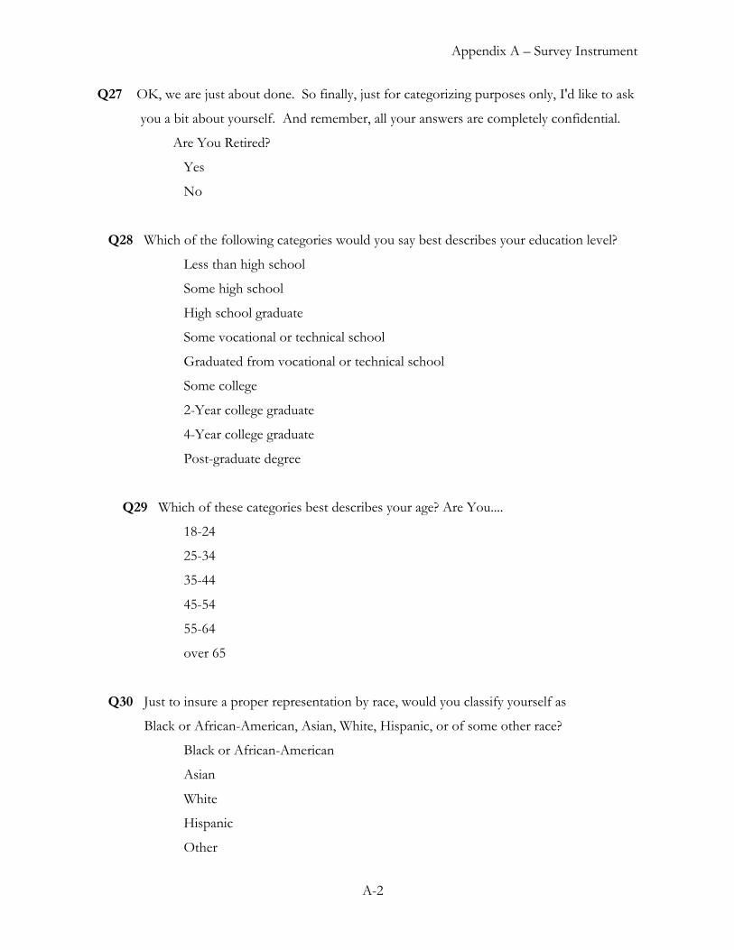
Q27 OK, we are just about done. So finally, just for categorizing purposes only, I'd like to ask
you a bit about yourself. And remember, all your answers are completely confidential.
Are You Retired?
Yes
No
Q28 Which of the following categories would you say best describes your education level?
Less than high school
Some high school
High school graduate
Some vocational or technical school
Graduated from vocational or technical school
Some college
2-Year college graduate
4-Year college graduate
Post-graduate degree
Q29 Which of these categories best describes your age? Are You....
18-24
25-34
35-44
45-54
55-64
over 65
Q30 Just to insure a proper representation by race, would you classify yourself as
Black or African-American, Asian, White, Hispanic, or of some other race?
Black or African-American
Asian
White
Hispanic
Other
A-2

Appendix A – Survey Instrument
Q31 Remember that none of this information can ever be associated with your name
or household, can you tell me which of the following categories best describes
your annual household income before taxes. Was it....
Less than $12,000
$12,000 to $25,000
$25,000 to $35,000
$35,000 to $50,000
$50,000 to $75,000
$75,000 to $100,000
over $100,000
Those are all the questions I have for you today.
Thank you for participating in this important survey.
A-3

Appendix B – Frequency Tables
B - 1
Appendix B Frequency Tables
Area
Frequency Percent Valid Percent Cumulative Percent Urban 267 26.7 26.7 26.7
Suburban 387 38.7 38.7 65.4
Rural 346 34.6 34.6 100.0Valid
Total 1000 100.0 100.0 May I speak to a person in the home that is 18 years of age or older?
Frequency Percent Valid Percent Cumulative Percent
Valid Yes I have someone on the line that is 18 years old or older
1000 100.0 100.0 100.0
Record gender of respondent.
Frequency Percent Valid Percent Cumulative Percent Female 600 60.0 60.0 60.0
Male 400 40.0 40.0 100.0Valid
Total 1000 100.0 100.0 Based on your current knowledge, do you think the overall water quality of the river, streams
and lakes in your area are
Frequency Percent Valid Percent Cumulative Percent Poor 132 13.2 13.2 13.2
Fair 394 39.4 39.4 52.6
Good 424 42.4 42.4 95.0
Excellent 29 2.9 2.9 97.9
Refuse to answer 21 2.1 2.1 100.0
Valid
Total 1000 100.0 100.0

Appendix B – Frequency Tables
B - 2
Wastewater from manufacturing plants - importance as a source of water pollution
Frequency Percent Valid Percent Cumulative Percent Very important 633 63.3 63.3 63.3
Important 284 28.4 28.4 91.7
Not important 61 6.1 6.1 97.8
Refuse to answer 22 2.2 2.2 100.0
Valid
Total 1000 100.0 100.0
Wastewater from sewer treatment plants - importance as a source of water pollution
Frequency Percent Valid Percent Cumulative Percent Very important 633 63.3 63.3 63.3
Important 277 27.7 27.7 91.0
Not important 76 7.6 7.6 98.6
Refuse to answer 14 1.4 1.4 100.0
Valid
Total 1000 100.0 100.0
Pollutants that wash out of the air (acid rain) - importance as a source of water pollution
Frequency Percent Valid Percent Cumulative Percent Very important 299 29.9 29.9 29.9
Important 523 52.3 52.3 82.2
Not important 143 14.3 14.3 96.5
Don't know 1 .1 .1 96.6
Refuse to answer 34 3.4 3.4 100.0
Valid
Total 1000 100.0 100.0
Rainfall runoff from yards, parking lots, and streets - importance as a source of water pollution
Frequency Percent Valid Percent Cumulative Percent Very important 247 24.7 24.7 24.7
Important 458 45.8 45.8 70.5
Not important 287 28.7 28.7 99.2
Refuse to answer 8 .8 .8 100.0
Valid
Total 1000 100.0 100.0

Appendix B – Frequency Tables
B - 3
Rainfall runoff from farms and agricultural operations - importance as a source of water pollution
Frequency Percent Valid Percent Cumulative Percent Very important 435 43.5 43.5 43.5
Important 416 41.6 41.6 85.1
Not important 128 12.8 12.8 97.9
Refuse to answer 21 2.1 2.1 100.0
Valid
Total 1000 100.0 100.0 Dirt eroding from construction sites - importance as a source of water pollution
Frequency Percent Valid Percent Cumulative Percent Very important 258 25.8 25.8 25.8
Important 497 49.7 49.7 75.5
Not important 234 23.4 23.4 98.9
Refuse to answer 11 1.1 1.1 100.0
Valid
Total 1000 100.0 100.0 Trash dumped into lakes and rivers by boaters and other recreactional users – importance as a source of water pollution
Frequency Percent Valid Percent Cumulative Percent Very important 674 67.4 67.4 67.4
Important 260 26.0 26.0 93.4
Not important 59 5.9 5.9 99.3
Don't know 1 .1 .1 99.4
Refuse to answer 6 .6 .6 100.0
Valid
Total 1000 100.0 100.0

Appendix B – Frequency Tables
B - 4
Which of the sources that you indicated as important or very important do you think is the most important as a source of water pollution?
Frequency Percent Valid Percent Cumulative Percent Manufacturing plants wastewater 309 30.9 30.9 30.9
Sewer treatment plants wastewater 192 19.2 19.2 50.2
Pollutants that wash out of the air (acid rain) 36 3.6 3.6 53.8
Rainfall runoff from yards, parking lots, and streets 45 4.5 4.5 58.3
Rainfall runoff from farms and agricultural operations 119 11.9 11.9 70.2
Construction site dirt erosion 33 3.3 3.3 73.5
Trash dumped into lakes and rivers 244 24.4 24.4 97.9
Don't know 2 .2 .2 98.1Refuse to answer 19 1.9 1.9 100.0
Valid
Total 999 99.9 100.0 Missing System 1 .1 Total 1000 100.0
Do you have a grass, lawn, or yard that you mow?
Frequency Percent Valid Percent Cumulative Percent Yes 961 96.1 96.1 96.1
No 38 3.8 3.8 99.9
Refuse to answer 1 .1 .1 100.0Valid
Total 1000 100.0 100.0
When you mow your grass, what do you do with the grass clippings?
Frequency Percent Valid Percent Cumulative Percent Leave them in the yard 469 46.9 53.7 53.7
Collect them and throw them in the garbage 228 22.8 26.1 79.7
Rake or blow them into a drain 13 1.3 1.5 81.2
Mulch or compost them 143 14.3 16.4 97.6
Something else 14 1.4 1.6 99.2
Refuse to answer 7 .7 .8 100.0
Valid
Total 874 87.4 100.0
Missing System 126 12.6
Total 1000 100.0

Appendix B – Frequency Tables
B - 5
Do you use fertilizer on your lawn?
Frequency Percent Valid Percent Cumulative Percent Yes 360 36.0 48.6 48.6
No 375 37.5 50.6 99.2
Refuse to answer 6 .6 .8 100.0Valid
Total 741 74.1 100.0
Missing System 259 25.9
Total 1000 100.0 About how often would you say you use fertilizer on your lawn?
Frequency Percent Valid Percent Cumulative Percent Monthly 21 2.1 5.8 5.8
Two or three times a year 167 16.7 46.1 51.9
Once a year or less 168 16.8 46.4 98.3
Refuse to answer 6 .6 1.7 100.0
Valid
Total 362 36.2 100.0 Missing System 638 63.8
Total 1000 100.0 Does anyone ever test the soil on your lawn to determine how much fertilizer is needed?
Frequency Percent Valid Percent Cumulative Percent Yes 161 16.1 44.1 44.1
No 198 19.8 54.2 98.4
Refuse to answer 6 .6 1.6 100.0Valid
Total 365 36.5 100.0
Missing System 635 63.5
Total 1000 100.0 Do you have a car/truck or other vehicle?
Frequency Percent Valid Percent Cumulative Percent
Yes 742 74.2 89.8 89.8
No 84 8.4 10.2 100.0Valid
Total 826 82.6 100.0
Missing System 174 17.4
Total 1000 100.0
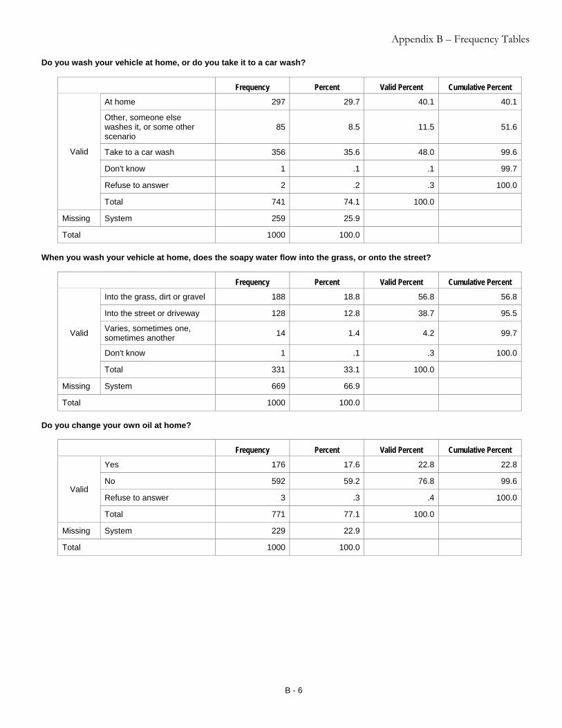
Appendix B – Frequency Tables
B - 6
Do you wash your vehicle at home, or do you take it to a car wash?
Frequency Percent Valid Percent Cumulative Percent At home 297 29.7 40.1 40.1
Other, someone else washes it, or some other scenario
85 8.5 11.5 51.6
Take to a car wash 356 35.6 48.0 99.6
Don't know 1 .1 .1 99.7
Refuse to answer 2 .2 .3 100.0
Valid
Total 741 74.1 100.0
Missing System 259 25.9
Total 1000 100.0 When you wash your vehicle at home, does the soapy water flow into the grass, or onto the street?
Frequency Percent Valid Percent Cumulative Percent Into the grass, dirt or gravel 188 18.8 56.8 56.8
Into the street or driveway 128 12.8 38.7 95.5
Varies, sometimes one, sometimes another 14 1.4 4.2 99.7
Don't know 1 .1 .3 100.0
Valid
Total 331 33.1 100.0
Missing System 669 66.9
Total 1000 100.0 Do you change your own oil at home?
Frequency Percent Valid Percent Cumulative Percent Yes 176 17.6 22.8 22.8
No 592 59.2 76.8 99.6
Refuse to answer 3 .3 .4 100.0Valid
Total 771 77.1 100.0
Missing System 229 22.9
Total 1000 100.0

Appendix B – Frequency Tables
B - 7
When you change your oil at home, how do you dispose of the used oil?
Frequency Percent Valid Percent Cumulative Percent In a designated lawn area 22 2.2 12.3 12.3
With other garbage (dumpster, placed in trash bags, etc)
36 3.6 20.1 32.4
Pour it down a storm drain 16 1.6 8.9 41.3
Take it somewhere it can be recycled 91 9.1 50.8 92.2
Other 10 1.0 5.6 97.8Refuse to answer 4 .4 2.2 100.0
Valid
Total 179 17.9 100.0 Missing System 821 82.1 Total 1000 100.0
Do you walk your pet?
Frequency Percent Valid Percent Cumulative Percent Yes 557 55.7 55.8 55.8
No 263 26.3 26.4 82.2
No Pets 178 17.8 17.8 100.0Valid
Total 998 99.8 100.0
Missing System 2 .2
Total 1000 100.0 How often do you pick up their pet waste?
Frequency Percent Valid Percent Cumulative Percent Always 152 15.2 26.6 26.6
Often 31 3.1 5.4 32.0
Sometimes 68 6.8 11.9 44.0
Rarely 145 14.5 25.4 69.4
Never 156 15.6 27.3 96.7
Refuse to answer 19 1.9 3.3 100.0
Valid
Total 571 57.1 100.0 Missing System 429 42.9
Total 1000 100.0

Appendix B – Frequency Tables
B - 8
Where would you say storm water runoff goes once it enters a storm drain?
Frequency Percent Valid Percent Cumulative Percent The city's regular sewer treatment plant 152 15.2 21.3 21.3
A separate special sewer treatment plant 53 5.3 7.4 28.8
Nearby fields and yards 70 7.0 9.8 38.6
Closest river, stream, or lake 268 26.8 37.6 76.2
Drainage pond 94 9.4 13.2 89.3
Refuse to answer 76 7.6 10.7 100.0
Valid
Total 713 71.3 100.0
Missing System 287 28.7
Total 1000 100.0 Are you retired?
Frequency Percent Valid Percent Cumulative Percent Yes 266 26.6 32.0 32.0
No 471 47.1 56.6 88.6
Don't know 66 6.6 7.9 96.5
Refuse to answer 29 2.9 3.5 100.0
Valid
Total 832 83.2 100.0
Missing System 168 16.8
Total 1000 100.0

Appendix B – Frequency Tables
B - 9
Which of the following categories would you say best describes your education level?
Frequency Percent Valid Percent Cumulative Percent Less than high school 42 4.2 4.2 4.2
Some high school 113 11.3 11.4 15.6
High school graduate 233 23.3 23.5 39.2
Some vocational or technical school 100 10.0 10.1 49.2
Graduated from vocational or technical school 64 6.4 6.5 55.7
Some college 150 15.0 15.1 70.8
2-Year college graduate 58 5.8 5.9 76.7
4-Year college graduate 153 15.3 15.4 92.1
Post-graduate degree 78 7.8 7.9 100.0
Valid
Total 991 99.1 100.0
Missing System 9 .9
Total 1000 100.0 Which of these categories best describes your age?
Frequency Percent Valid Percent Cumulative Percent 18-24 108 10.8 10.8 10.8
25-34 81 8.1 8.1 18.9
35-44 313 31.3 31.3 50.3
45-54 177 17.7 17.7 68.0
55-64 137 13.7 13.7 81.7
Over 65 170 17.0 17.0 98.7
Don't know 13 1.3 1.3 100.0
Valid
Total 999 99.9 100.0
Missing System 1 .1
Total 1000 100.0

Appendix B – Frequency Tables
B - 10
How would you classify yourself?
Frequency Percent Valid Percent Cumulative Percent Black or African-American 166 16.6 17.1 17.1
Asian 37 3.7 3.8 20.9
White 537 53.7 55.4 76.4
Hispanic 87 8.7 9.0 85.3
Other 73 7.3 7.5 92.9
Don't know 59 5.9 6.1 99.0
Refuse to answer 10 1.0 1.0 100.0
Valid
Total 969 96.9 100.0
Missing System 31 3.1
Total 1000 100.0 Which of the following categories best describes your annual household income before taxes?
Frequency Less than $12,000 86
$12,000 to $25,000 99
$25,000 to $35,000 88
$35,000 to $50,000 99
$50,000 to $75,000 104
$75,000 to $100,000 56
Over $100,000 51
Don't know 107
Refuse to answer 23
Valid
Total 713
Missing System 287
Total 1000 Sources of Water Pollution
Of the sources of water pollution, 93.4% of respondents thought that recreational trash was important/very important.
91.7% indicated that manufacturing wastewater was important/very important and 91% indicated that wastewater from
sewer treatment plants was important/very important. These were the same top three issues that surfaced as the MOST
important sources of water pollution (999 total).
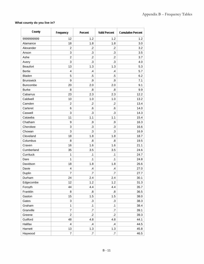
Appendix B – Frequency Tables
B - 11
What county do you live in?
County Frequency Percent Valid Percent Cumulative Percent
9999999999 12 1.2 1.2 1.2Alamance 18 1.8 1.8 3.0Alexander 2 .2 .2 3.2Anson 3 .3 .3 3.5Ashe 2 .2 .2 3.7Avery 3 .3 .3 4.0Beaufort 13 1.3 1.3 5.3Bertie 4 .4 .4 5.7Bladen 5 .5 .5 6.2Brunswick 9 .9 .9 7.1Buncombe 20 2.0 2.0 9.1Burke 8 .8 .8 9.9Cabarrus 23 2.3 2.3 12.2Caldwell 10 1.0 1.0 13.2Camden 2 .2 .2 13.4Carteret 6 .6 .6 14.0Caswell 3 .3 .3 14.3Catawba 11 1.1 1.1 15.4Chatham 9 .9 .9 16.3Cherokee 3 .3 .3 16.6Chowan 3 .3 .3 16.9Cleveland 18 1.8 1.8 18.7Columbus 8 .8 .8 19.5Craven 16 1.6 1.6 21.1Cumberland 35 3.5 3.5 24.6Currituck 1 .1 .1 24.7Dare 1 .1 .1 24.8Davidson 18 1.8 1.8 26.6Davie 4 .4 .4 27.0Duplin 7 .7 .7 27.7Durham 24 2.4 2.4 30.1Edgecombe 12 1.2 1.2 31.3Forsyth 44 4.4 4.4 35.7Franklin 8 .8 .8 36.5Gaston 15 1.5 1.5 38.0Gates 3 .3 .3 38.3Graham 1 .1 .1 38.4Granville 7 .7 .7 39.1Greene 2 .2 .2 39.3Guilford 48 4.8 4.8 44.1Halifax 4 .4 .4 44.5Harnett 13 1.3 1.3 45.8Haywood 7 .7 .7 46.5

Appendix B – Frequency Tables
B - 12
County Frequency Percent Valid Percent Cumulative Percent
Henderson 8 .8 .8 47.3Hertford 6 .6 .6 47.9Hoke 9 .9 .9 48.8Iredell 9 .9 .9 49.7Jackson 2 .2 .2 49.9Johnston 14 1.4 1.4 51.3Lee 3 .3 .3 51.6Lenoir 11 1.1 1.1 52.7Lincoln 5 .5 .5 53.2Macon 5 .5 .5 53.7Madison 3 .3 .3 54.0Mcdowell 4 .4 .4 54.4Mecklenburg 56 5.6 5.6 60.0Mitchell 2 .2 .2 60.2Montgomery 1 .1 .1 60.3Moore 9 .9 .9 61.2Nash 10 1.0 1.0 62.2New Hanover 16 1.6 1.6 63.8Northampton 5 .5 .5 64.3Onslow 21 2.1 2.1 66.4Orange 5 .5 .5 66.9Pamlico 2 .2 .2 67.1Pasquotank 5 .5 .5 67.6Pender 6 .6 .6 68.2Perquimans 2 .2 .2 68.4Person 5 .5 .5 68.9Pitt 20 2.0 2.0 70.9Polk 3 .3 .3 71.2Randolph 13 1.3 1.3 72.5Richmond 6 .6 .6 73.1Robeson 17 1.7 1.7 74.8Rockingham 13 1.3 1.3 76.1Rowan 13 1.3 1.3 77.4Rutherford 2 .2 .2 77.6Sampson 18 1.8 1.8 79.4Scotland 3 .3 .3 79.7Stanly 2 .2 .2 79.9Stokes 6 .6 .6 80.5Surry 10 1.0 1.0 81.5Swain 2 .2 .2 81.7Transylvania 5 .5 .5 82.2Union 19 1.9 1.9 84.1Vance 10 1.0 1.0 85.1Wake 94 9.4 9.4 94.5Warren 4 .4 .4 94.9

Appendix B – Frequency Tables
B - 13
County Frequency Percent Valid Percent Cumulative Percent
Washington 2 .2 .2 95.1Watauga 5 .5 .5 95.6Wayne 17 1.7 1.7 97.3Wilkes 5 .5 .5 97.8Wilson 15 1.5 1.5 99.3Yadkin 4 .4 .4 99.7Yancey 3 .3 .3 100.0Total 1000 100.0 100.0

Appendix B – Frequency Tables
B - 14
What is your zip code?
Zip Code Frequency Percent Valid Percent Cumulative Percent
27010 1 .1 .1 .127011 1 .1 .1 .227012 6 .6 .6 .827013 1 .1 .1 .927014 1 .1 .1 1.027017 2 .2 .2 1.227018 1 .1 .1 1.327020 1 .1 .1 1.427021 1 .1 .1 1.527022 1 .1 .1 1.627024 1 .1 .1 1.727025 1 .1 .1 1.827028 3 .3 .3 2.127030 4 .4 .4 2.527036 1 .1 .1 2.627041 1 .1 .1 2.727043 1 .1 .1 2.827048 2 .2 .2 3.027051 4 .4 .4 3.427052 1 .1 .1 3.527053 2 .2 .2 3.727055 1 .1 .1 3.827101 3 .3 .3 4.127103 3 .3 .3 4.427104 3 .3 .3 4.727105 2 .2 .2 4.927106 5 .5 .5 5.427107 4 .4 .4 5.827127 2 .2 .2 6.027203 2 .2 .2 6.227204 2 .2 .2 6.427205 2 .2 .2 6.627209 1 .1 .1 6.727214 1 .1 .1 6.827215 7 .7 .7 7.527217 5 .5 .5 8.027230 1 .1 .1 8.127235 1 .1 .1 8.227239 1 .1 .1 8.327249 1 .1 .1 8.427253 5 .5 .5 8.927263 1 .1 .1 9.027269 1 .1 .1 9.1

Appendix B – Frequency Tables
B - 15
Zip Code Frequency Percent Valid Percent Cumulative Percent
27278 1 .1 .1 9.227281 1 .1 .1 9.327283 1 .1 .1 9.427284 8 .8 .8 10.227285 1 .1 .1 10.327288 3 .3 .3 10.627292 4 .4 .4 11.027293 1 .1 .1 11.127295 3 .3 .3 11.427297 1 .1 .1 11.527299 2 .2 .2 11.727301 1 .1 .1 11.827302 2 .2 .2 12.027310 1 .1 .1 12.127312 5 .5 .5 12.627314 1 .1 .1 12.727316 1 .1 .1 12.827317 1 .1 .1 12.927320 4 .4 .4 13.327330 3 .3 .3 13.627341 1 .1 .1 13.727344 3 .3 .3 14.027357 1 .1 .1 14.127360 2 .2 .2 14.327361 1 .1 .1 14.427370 2 .2 .2 14.627379 1 .1 .1 14.727401 3 .3 .3 15.027403 6 .6 .6 15.627405 5 .5 .5 16.127406 2 .2 .2 16.327407 6 .6 .6 16.927408 1 .1 .1 17.027409 1 .1 .1 17.127410 5 .5 .5 17.627420 1 .1 .1 17.727425 1 .1 .1 17.827429 1 .1 .1 17.927435 1 .1 .1 18.027455 4 .4 .4 18.427491 1 .1 .1 18.527495 1 .1 .1 18.627501 2 .2 .2 18.827502 3 .3 .3 19.127503 1 .1 .1 19.2

Appendix B – Frequency Tables
B - 16
Zip Code Frequency Percent Valid Percent Cumulative Percent
27509 2 .2 .2 19.427510 1 .1 .1 19.527511 3 .3 .3 19.827513 5 .5 .5 20.327515 2 .2 .2 20.527516 1 .1 .1 20.627519 3 .3 .3 20.927520 3 .3 .3 21.227521 1 .1 .1 21.327522 3 .3 .3 21.627524 3 .3 .3 21.927525 3 .3 .3 22.227526 4 .4 .4 22.627527 1 .1 .1 22.727529 3 .3 .3 23.027530 4 .4 .4 23.427531 1 .1 .1 23.527534 1 .1 .1 23.627536 7 .7 .7 24.327537 3 .3 .3 24.627540 4 .4 .4 25.027541 1 .1 .1 25.127545 3 .3 .3 25.427546 4 .4 .4 25.827549 3 .3 .3 26.127552 1 .1 .1 26.227557 3 .3 .3 26.527560 5 .5 .5 27.027562 1 .1 .1 27.127565 1 .1 .1 27.227569 2 .2 .2 27.427571 1 .1 .1 27.527572 1 .1 .1 27.627573 1 .1 .1 27.727574 2 .2 .2 27.927576 1 .1 .1 28.027577 2 .2 .2 28.227581 1 .1 .1 28.327583 1 .1 .1 28.427587 9 .9 .9 29.327588 1 .1 .1 29.427589 2 .2 .2 29.627591 1 .1 .1 29.727592 3 .3 .3 30.027594 1 .1 .1 30.1

Appendix B – Frequency Tables
B - 17
Zip Code Frequency Percent Valid Percent Cumulative Percent
27596 2 .2 .2 30.327601 1 .1 .1 30.427602 1 .1 .1 30.527603 7 .7 .7 31.227604 5 .5 .5 31.727607 2 .2 .2 31.927608 1 .1 .1 32.027609 3 .3 .3 32.327610 5 .5 .5 32.827612 1 .1 .1 32.927613 4 .4 .4 33.327614 1 .1 .1 33.427615 2 .2 .2 33.627616 3 .3 .3 33.927617 2 .2 .2 34.127620 1 .1 .1 34.227701 3 .3 .3 34.527703 4 .4 .4 34.927704 1 .1 .1 35.027705 2 .2 .2 35.227707 4 .4 .4 35.627712 2 .2 .2 35.827713 2 .2 .2 36.027717 4 .4 .4 36.427801 1 .1 .1 36.527803 3 .3 .3 36.827804 1 .1 .1 36.927806 2 .2 .2 37.127809 1 .1 .1 37.227812 1 .1 .1 37.327814 1 .1 .1 37.427821 1 .1 .1 37.527822 1 .1 .1 37.627826 1 .1 .1 37.727830 1 .1 .1 37.827831 2 .2 .2 38.027832 1 .1 .1 38.127834 10 1.0 1.0 39.127839 1 .1 .1 39.227852 2 .2 .2 39.427853 1 .1 .1 39.527854 1 .1 .1 39.627855 2 .2 .2 39.827856 2 .2 .2 40.027858 10 1.0 1.0 41.0

Appendix B – Frequency Tables
B - 18
Zip Code Frequency Percent Valid Percent Cumulative Percent
27862 1 .1 .1 41.127863 3 .3 .3 41.427864 3 .3 .3 41.727865 1 .1 .1 41.827870 2 .2 .2 42.027873 1 .1 .1 42.127882 3 .3 .3 42.427886 5 .5 .5 42.927889 8 .8 .8 43.727893 6 .6 .6 44.327896 2 .2 .2 44.527906 1 .1 .1 44.627907 1 .1 .1 44.727909 4 .4 .4 45.127910 3 .3 .3 45.427920 1 .1 .1 45.527921 1 .1 .1 45.627922 1 .1 .1 45.727924 1 .1 .1 45.827926 1 .1 .1 45.927928 1 .1 .1 46.027932 2 .2 .2 46.227935 1 .1 .1 46.327937 1 .1 .1 46.427944 1 .1 .1 46.527962 1 .1 .1 46.627976 1 .1 .1 46.727980 1 .1 .1 46.827983 2 .2 .2 47.028001 1 .1 .1 47.128018 1 .1 .1 47.228020 1 .1 .1 47.328025 8 .8 .8 48.128026 1 .1 .1 48.228027 7 .7 .7 48.928031 2 .2 .2 49.128033 1 .1 .1 49.228036 1 .1 .1 49.328046 1 .1 .1 49.428051 1 .1 .1 49.528052 3 .3 .3 49.828054 4 .4 .4 50.228056 1 .1 .1 50.328073 1 .1 .1 50.428075 2 .2 .2 50.6

Appendix B – Frequency Tables
B - 19
Zip Code Frequency Percent Valid Percent Cumulative Percent
28078 5 .5 .5 51.128079 1 .1 .1 51.228080 3 .3 .3 51.528081 4 .4 .4 51.928086 3 .3 .3 52.228088 1 .1 .1 52.328090 1 .1 .1 52.428092 2 .2 .2 52.628103 2 .2 .2 52.828104 5 .5 .5 53.328105 2 .2 .2 53.528107 1 .1 .1 53.628110 3 .3 .3 53.928111 1 .1 .1 54.028112 2 .2 .2 54.228114 1 .1 .1 54.328115 3 .3 .3 54.628119 1 .1 .1 54.728120 4 .4 .4 55.128127 1 .1 .1 55.228133 1 .1 .1 55.328134 2 .2 .2 55.528139 1 .1 .1 55.628144 3 .3 .3 55.928146 2 .2 .2 56.128147 5 .5 .5 56.628150 6 .6 .6 57.228152 3 .3 .3 57.528164 1 .1 .1 57.628166 1 .1 .1 57.728168 1 .1 .1 57.828169 1 .1 .1 57.928170 1 .1 .1 58.028173 6 .6 .6 58.628202 1 .1 .1 58.728204 1 .1 .1 58.828205 4 .4 .4 59.228208 2 .2 .2 59.428209 1 .1 .1 59.528210 4 .4 .4 59.928211 2 .2 .2 60.128212 2 .2 .2 60.328213 1 .1 .1 60.428214 1 .1 .1 60.528215 2 .2 .2 60.7
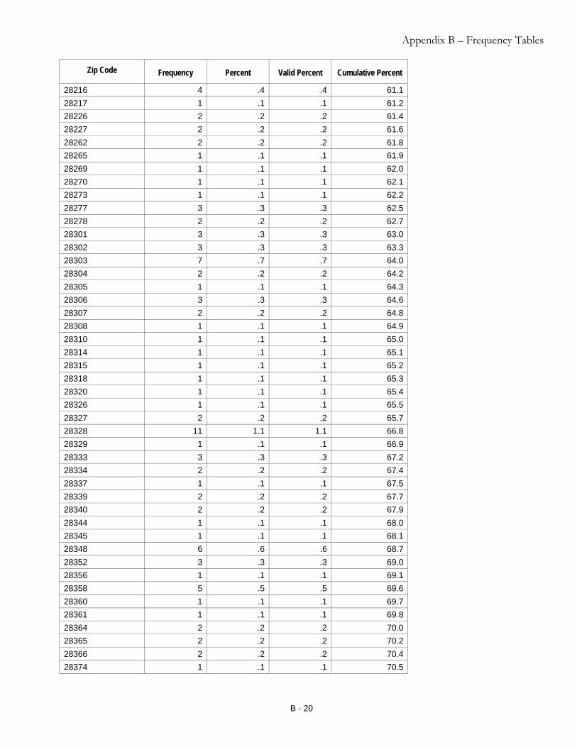
Appendix B – Frequency Tables
B - 20
Zip Code Frequency Percent Valid Percent Cumulative Percent
28216 4 .4 .4 61.128217 1 .1 .1 61.228226 2 .2 .2 61.428227 2 .2 .2 61.628262 2 .2 .2 61.828265 1 .1 .1 61.928269 1 .1 .1 62.028270 1 .1 .1 62.128273 1 .1 .1 62.228277 3 .3 .3 62.528278 2 .2 .2 62.728301 3 .3 .3 63.028302 3 .3 .3 63.328303 7 .7 .7 64.028304 2 .2 .2 64.228305 1 .1 .1 64.328306 3 .3 .3 64.628307 2 .2 .2 64.828308 1 .1 .1 64.928310 1 .1 .1 65.028314 1 .1 .1 65.128315 1 .1 .1 65.228318 1 .1 .1 65.328320 1 .1 .1 65.428326 1 .1 .1 65.528327 2 .2 .2 65.728328 11 1.1 1.1 66.828329 1 .1 .1 66.928333 3 .3 .3 67.228334 2 .2 .2 67.428337 1 .1 .1 67.528339 2 .2 .2 67.728340 2 .2 .2 67.928344 1 .1 .1 68.028345 1 .1 .1 68.128348 6 .6 .6 68.728352 3 .3 .3 69.028356 1 .1 .1 69.128358 5 .5 .5 69.628360 1 .1 .1 69.728361 1 .1 .1 69.828364 2 .2 .2 70.028365 2 .2 .2 70.228366 2 .2 .2 70.428374 1 .1 .1 70.5

Appendix B – Frequency Tables
B - 21
Zip Code Frequency Percent Valid Percent Cumulative Percent
28376 8 .8 .8 71.328377 1 .1 .1 71.428379 3 .3 .3 71.728384 3 .3 .3 72.028385 1 .1 .1 72.128386 2 .2 .2 72.328387 2 .2 .2 72.528390 3 .3 .3 72.828393 1 .1 .1 72.928394 1 .1 .1 73.028401 1 .1 .1 73.128403 2 .2 .2 73.328405 2 .2 .2 73.528409 2 .2 .2 73.728411 3 .3 .3 74.028412 5 .5 .5 74.528420 1 .1 .1 74.628423 1 .1 .1 74.728424 1 .1 .1 74.828425 1 .1 .1 74.928431 1 .1 .1 75.028433 2 .2 .2 75.228434 1 .1 .1 75.328441 1 .1 .1 75.428443 3 .3 .3 75.728445 1 .1 .1 75.828451 1 .1 .1 75.928453 1 .1 .1 76.028457 1 .1 .1 76.128458 1 .1 .1 76.228460 2 .2 .2 76.428461 1 .1 .1 76.528462 1 .1 .1 76.628463 3 .3 .3 76.928464 1 .1 .1 77.028466 2 .2 .2 77.228467 3 .3 .3 77.528468 1 .1 .1 77.628470 1 .1 .1 77.728472 1 .1 .1 77.828478 1 .1 .1 77.928501 2 .2 .2 78.128502 1 .1 .1 78.228504 4 .4 .4 78.628508 1 .1 .1 78.7

Appendix B – Frequency Tables
B - 22
Zip Code Frequency Percent Valid Percent Cumulative Percent
28512 1 .1 .1 78.828516 1 .1 .1 78.928523 1 .1 .1 79.028526 2 .2 .2 79.228529 1 .1 .1 79.328532 4 .4 .4 79.728536 1 .1 .1 79.828539 3 .3 .3 80.128540 6 .6 .6 80.728541 1 .1 .1 80.828546 3 .3 .3 81.128547 2 .2 .2 81.328551 2 .2 .2 81.528557 1 .1 .1 81.628560 4 .4 .4 82.028562 4 .4 .4 82.428570 3 .3 .3 82.728572 3 .3 .3 83.028574 2 .2 .2 83.228578 1 .1 .1 83.328580 1 .1 .1 83.428584 1 .1 .1 83.528586 1 .1 .1 83.628601 4 .4 .4 84.028602 3 .3 .3 84.328604 1 .1 .1 84.428605 1 .1 .1 84.528607 3 .3 .3 84.828610 1 .1 .1 84.928612 1 .1 .1 85.028613 1 .1 .1 85.128618 1 .1 .1 85.228621 2 .2 .2 85.428622 1 .1 .1 85.528625 1 .1 .1 85.628626 2 .2 .2 85.828630 2 .2 .2 86.028633 1 .1 .1 86.128637 1 .1 .1 86.228638 1 .1 .1 86.328645 6 .6 .6 86.928650 1 .1 .1 87.028655 6 .6 .6 87.628659 3 .3 .3 87.928673 1 .1 .1 88.0

Appendix B – Frequency Tables
B - 23
Zip Code Frequency Percent Valid Percent Cumulative Percent
28677 4 .4 .4 88.428681 2 .2 .2 88.628685 2 .2 .2 88.828701 1 .1 .1 88.928704 1 .1 .1 89.028705 1 .1 .1 89.128712 2 .2 .2 89.328713 2 .2 .2 89.528714 3 .3 .3 89.828715 3 .3 .3 90.128716 1 .1 .1 90.228717 1 .1 .1 90.328718 1 .1 .1 90.428722 1 .1 .1 90.528730 1 .1 .1 90.628731 1 .1 .1 90.728732 1 .1 .1 90.828734 3 .3 .3 91.128737 1 .1 .1 91.228742 1 .1 .1 91.328744 1 .1 .1 91.428745 1 .1 .1 91.528748 1 .1 .1 91.628751 2 .2 .2 91.828752 2 .2 .2 92.028754 3 .3 .3 92.328756 1 .1 .1 92.428762 1 .1 .1 92.528763 1 .1 .1 92.628768 1 .1 .1 92.728771 1 .1 .1 92.828772 1 .1 .1 92.928778 1 .1 .1 93.028779 1 .1 .1 93.128782 1 .1 .1 93.228786 3 .3 .3 93.528787 3 .3 .3 93.828791 1 .1 .1 93.928792 4 .4 .4 94.328801 2 .2 .2 94.528802 1 .1 .1 94.628803 1 .1 .1 94.728804 1 .1 .1 94.828805 1 .1 .1 94.928807 1 .1 .1 95.0

Appendix B – Frequency Tables
B - 24
Zip Code Frequency Percent Valid Percent Cumulative Percent
28816 1 .1 .1 95.128880 1 .1 .1 95.228905 1 .1 .1 95.328906 2 .2 .2 95.599998 1 .1 .1 95.699999 44 4.4 4.4 100.0Total 1000 100.0 100.0
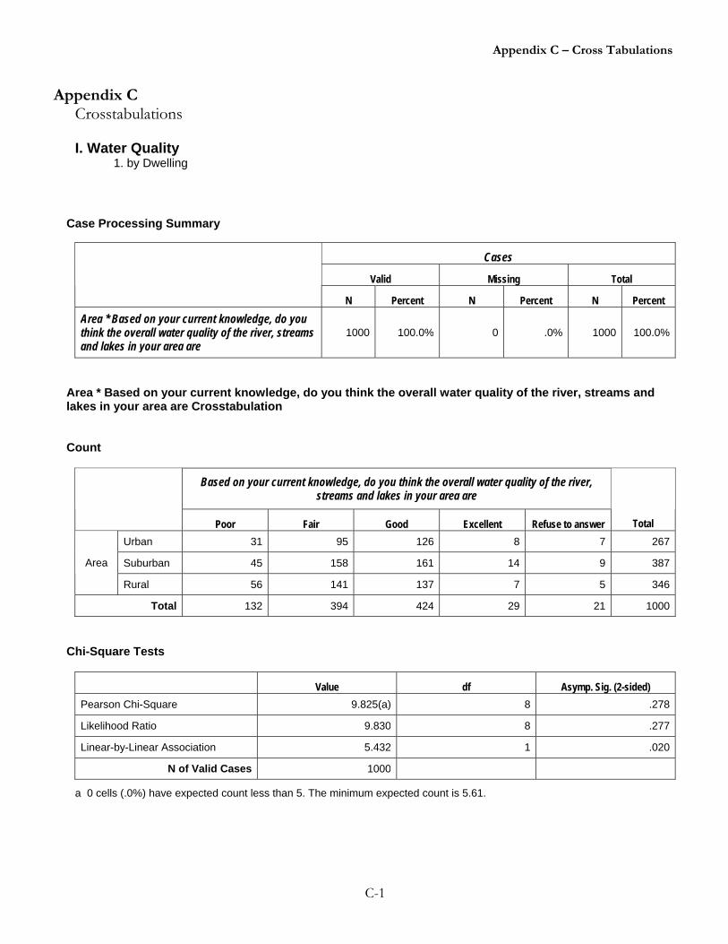
Appendix C – Cross Tabulations
C-1
Appendix C Crosstabulations I. Water Quality 1. by Dwelling
Case Processing Summary
Cases
Valid Missing Total
N Percent N Percent N Percent Area * Based on your current knowledge, do you think the overall water quality of the river, streams and lakes in your area are
1000 100.0% 0 .0% 1000 100.0%
Area * Based on your current knowledge, do you think the overall water quality of the river, streams and lakes in your area are Crosstabulation Count
Based on your current knowledge, do you think the overall water quality of the river, streams and lakes in your area are
Poor Fair Good Excellent Refuse to answer Total Urban 31 95 126 8 7 267
Suburban 45 158 161 14 9 387Area
Rural 56 141 137 7 5 346
Total 132 394 424 29 21 1000
Chi-Square Tests
Value df Asymp. Sig. (2-sided) Pearson Chi-Square 9.825(a) 8 .278
Likelihood Ratio 9.830 8 .277
Linear-by-Linear Association 5.432 1 .020
N of Valid Cases 1000
a 0 cells (.0%) have expected count less than 5. The minimum expected count is 5.61.

Appendix C – Cross Tabulations
C-2
Directional Measures
Value Area Dependent .085
Nominal by Interval Eta Based on your current knowledge, do you think the overall water quality of the river, streams and lakes in your area are Dependent .076
Symmetric Measures
Value Approx. Sig. Phi .099 .278
Cramer's V .070 .278Nominal by Nominal
Contingency Coefficient .099 .278
N of Valid Cases 1000
a Not assuming the null hypothesis.
b Using the asymptotic standard error assuming the null hypothesis.
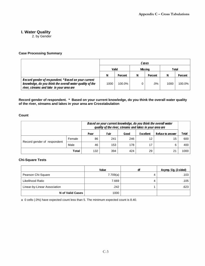
Appendix C – Cross Tabulations
C-3
I. Water Quality 2. by Gender
Case Processing Summary
Cases
Valid Missing Total
N Percent N Percent N Percent Record gender of respondent. * Based on your current knowledge, do you think the overall water quality of the river, streams and lake in your area are
1000 100.0% 0 .0% 1000 100.0%
Record gender of respondent. * Based on your current knowledge, do you think the overall water quality of the river, streams and lakes in your area are Crosstabulation Count
Based on your current knowledge, do you think the overall water quality of the river, streams and lakes in your area are
Poor Fair Good Excellent Refuse to answer Total Female 86 241 246 12 15 600
Record gender of respondent Male 46 153 178 17 6 400
Total 132 394 424 29 21 1000
Chi-Square Tests
Value df Asymp. Sig. (2-sided) Pearson Chi-Square 7.709(a) 4 .103
Likelihood Ratio 7.669 4 .105
Linear-by-Linear Association .242 1 .623
N of Valid Cases 1000
a 0 cells (.0%) have expected count less than 5. The minimum expected count is 8.40.

Appendix C – Cross Tabulations
C-4
Directional Measures
Value Record gender of respondent. Dependent .088
Nominal by Interval Eta Based on your current knowledge, do you think the overall water quality of the river, streams and lakes in your area are Dependent .016
Symmetric Measures
Value Approx. Sig. Phi .088 .103
Cramer's V .088 .103Nominal by Nominal
Contingency Coefficient .087 .103
N of Valid Cases 1000
a Not assuming the null hypothesis.
b Using the asymptotic standard error assuming the null hypothesis.

Appendix C – Cross Tabulations
C-5
I. Water Quality 3. by Retirement Status
Case Processing Summary
Cases
Valid Missing Total
N Percent N Percent N Percent
Are you retired? * Based on your current knowledge, do you think the overall water quality of the river, streams and lakes in your area are
832 83.2% 168 16.8% 1000 100.0%
Are you retired? * Based on your current knowledge, do you think the overall water quality of the river, streams and lakes in your area are Crosstabulation Count
Based on your current knowledge, do you think the overall water quality of the river, streams and lakes in your area are
Poor Fair Good Excellent Refuse to answer Total
Are you retired?
Yes 54 96 97 8 11 266
No 53 203 198 10 7 471
Don't know 4 29 30 3 0 66
Refuse to answer 4 9 14 1 1 29
Total 115 337 339 22 19 832
Chi-Square Tests
Value df Asymp. Sig. (2-sided) Pearson Chi-Square 26.827(a) 12 .008
Likelihood Ratio 27.566 12 .006
Linear-by-Linear Association .134 1 .714
N of Valid Cases 832
a 5 cells (25.0%) have expected count less than 5. The minimum expected count is .66.

Appendix C – Cross Tabulations
C-6
Directional Measures
Value Are you retired? Dependent .096
Nominal by Interval Eta Based on your current knowledge, do you think the overall water quality of the river, streams and lakes in your area are Dependent .034
Symmetric Measures
Value Approx. Sig. Phi .180 .008
Cramer's V .104 .008Nominal by Nominal
Contingency Coefficient .177 .008
N of Valid Cases 832
a Not assuming the null hypothesis.
b Using the asymptotic standard error assuming the null hypothesis.

Appendix C – Cross Tabulations
C-7
I. Water Quality 4. by Education
Case Processing Summary
Cases
Valid Missing Total
N Percent N Percent N Percent Which of the following categories would you say best describes your education level? * Based on your current knowledge, do you think the overall water quality of the river, streams and lakes in your area are
991 99.1% 9 .9% 1000 100.0%
Which of the following categories would you say best describes your education level? * Based on your current knowledge, do you think the overall water quality of the river, streams and lakes in your area are Crosstabulation Count
Based on your current knowledge, do you think the overall water quality of the river, streams and lakes in your area are
Poor Fair Good Excellent Refuse to answer Total
Which of the following categories would you say best describes your education level?
Less than high school 4 17 19 2 0 42
Some high school 14 42 47 5 5 113
High school graduate 29 83 112 4 5 233
Some vocational or technical school 10 51 35 3 1 100
Graduated from vocational or technical school 6 19 31 4 4 64
Some college 27 53 63 4 3 150
2-Year college graduate 12 25 19 1 1 58
4-Year college graduate 20 70 59 3 1 153
Post-graduate degree 9 29 37 2 1 78
Total 131 389 422 28 21 991

Appendix C – Cross Tabulations
C-8
Chi-Square Tests
Value df Asymp. Sig. (2-sided) Pearson Chi-Square 39.003(a) 32 .184
Likelihood Ratio 37.005 32 .249
Linear-by-Linear Association 3.576 1 .059
N of Valid Cases 991
a 17 cells (37.8%) have expected count less than 5. The minimum expected count is .89. Directional Measures
Value Which of the following categories would you say best describes your education level? Dependent .063
Nominal by Interval Eta Based on your current knowledge, do you think the overall water quality of the river, streams and lakes in your area are Dependent .136
Symmetric Measures
Value Approx. Sig. Phi .198 .184
Cramer's V .099 .184Nominal by Nominal
Contingency Coefficient .195 .184
N of Valid Cases 991
a Not assuming the null hypothesis.

Appendix C – Cross Tabulations
C-9
I. Water Quality 5. By Age
Case Processing Summary
Cases
Valid Missing Total
N Percent N Percent N Percent Which of these categories best describes your age? * Based on your current knowledge, do you think the overall water quality of the river, streams and lakes in your area are
999 99.9% 1 .1% 1000 100.0%
Which of these categories best describes your age? * Based on your current knowledge, do you think the overall water quality of the river, streams and lakes in your area are Crosstabulation Count
Based on your current knowledge, do you think the overall water quality of the river, streams and lakes in your area are
Poor Fair Good Excellent Refuse to answer Total
Which of these categories best describes your age?
18-24 6 45 51 4 2 108
25-34 6 38 36 1 0 81
35-44 43 122 136 8 4 313
45-54 21 71 75 7 3 177
55-64 24 57 50 2 4 137
Over 65 30 53 73 6 8 170
Don't know 2 7 3 1 0 13
Total 132 393 424 29 21 999

Appendix C – Cross Tabulations
C-10
Chi-Square Tests
Value df Asymp. Sig. (2-sided) Pearson Chi-Square 32.957(a) 24 .105
Likelihood Ratio 35.304 24 .064
Linear-by-Linear Association .159 1 .690
N of Valid Cases 999
a 12 cells (34.3%) have expected count less than 5. The minimum expected count is .27. Directional Measures
Value
Which of these categories best describes your age? Dependent .127Nominal by Interval Eta
Based on your current knowledge, do you think the overall water quality of the river, streams and lakes in your area are Dependent .080
Symmetric Measures
Value Approx. Sig. Phi .182 .105
Cramer's V .091 .105Nominal by Nominal
Contingency Coefficient .179 .105
N of Valid Cases 999
a Not assuming the null hypothesis.

Appendix C – Cross Tabulations
C-11
I. Water Quality 6. By Race
Case Processing Summary
Cases
Valid Missing Total
N Percent N Percent N Percent How would you classify yourself? * Based on your current knowledge, do you think the overall water quality of the river, streams and lakes in your area are
969 96.9% 31 3.1% 1000 100.0%
How would you classify yourself? * Based on your current knowledge, do you think the overall water quality of the river, streams and lakes in your area are Crosstabulation Count
Based on your current knowledge, do you think the overall water quality of the river, streams and lakes in your area are
Poor Fair Good Excellent Refuse to answer Total
How would you classify yourself?
Black or African-American 27 63 66 6 4 166
Asian 3 14 18 1 1 37
White 69 218 229 11 10 537
Hispanic 9 29 43 6 0 87
Other 15 24 28 2 4 73
Don't know 7 25 23 3 1 59
Refuse to answer 0 5 5 0 0 10
Total 130 378 412 29 20 969

Appendix C – Cross Tabulations
C-12
Chi-Square Tests
Value df Asymp. Sig. (2-sided) Pearson Chi-Square 25.127(a) 24 .399
Likelihood Ratio 26.023 24 .352
Linear-by-Linear Association .102 1 .750
N of Valid Cases 969
a 16 cells (45.7%) have expected count less than 5. The minimum expected count is .21. Directional Measures
Value
How would you classify yourself? Dependent .029Nominal by Interval Eta
Based on your current knowledge, do you think the overall water quality of the river, streams and lakes in your area are Dependent .042
Symmetric Measures
Value Approx. Sig. Phi .161 .399
Cramer's V .081 .399Nominal by Nominal
Contingency Coefficient .159 .399
N of Valid Cases 969
a Not assuming the null hypothesis.

Appendix C – Cross Tabulations
C-13
I. Water Quality 7. By Income
Case Processing Summary
Cases
Valid Missing Total
N Percent N Percent N Percent Which of the following categories best describes your annual household income before taxes? * Based on your current knowledge, do you think the overall water quality of the river, streams and lakes in your area are
713 71.3% 287 28.7% 1000 100.0%
Which of the following categories best describes your annual household income before taxes? * Based on your current knowledge, do you think the overall water quality of the river, streams and lakes in your area are Cosstabulation Count
Based on your current knowledge, do you think the overall water quality of the river, streams and lakes in your area are
Poor Fair Good Excellent Refuse to answer Total
Which of the following categories best describes your annual household income before taxes?
Less than $12,000 20 28 29 6 3 86
$12,000 to $25,000 17 42 37 1 2 99
$25,000 to $35,000 11 36 37 3 1 88
$35,000 to $50,000 15 44 36 2 2 99
$50,000 to $75,000 13 42 46 2 1 104
$75,000 to $100,000 6 27 23 0 0 56
Over $100,000 3 20 27 1 0 51
Don't know 13 47 39 3 5 107
Refuse to answer 3 8 10 0 2 23
Total 101 294 284 18 16 713

Appendix C – Cross Tabulations
C-14
Chi-Square Tests
Value df Asymp. Sig. (2-sided) Pearson Chi-Square 38.466(a) 32 .200
Likelihood Ratio 38.501 32 .199
Linear-by-Linear Association 2.321 1 .128
N of Valid Cases 713
a 19 cells (42.2%) have expected count less than 5. The minimum expected count is .52. Directional Measures
Value Which of the following categories best describes your annual household income before taxes? Dependent .116
Nominal by Interval Eta Based on your current knowledge, do you think the overall water quality of the river, streams and lakes in your area are Dependent .099
Symmetric Measures
Value Approx. Sig. Phi .232 .200
Cramer's V .116 .200Nominal by Nominal
Contingency Coefficient .226 .200
N of Valid Cases 713
a Not assuming the null hypothesis.
b Using the asymptotic standard error assuming the null hypothesis.

Appendix C – Cross Tabulations
C-15
II. Where Stormwater Goes 1. by Age
Where would you say storm water runoff goes once it enters a storm drain? * Which of these categories best describes your age? Crosstabulation Count
Which of these categories best describes your age?
18-24 25-34 35-44 45-54 55-64 Over 65 Don't know Total
Where would you say storm water runoff goes once it enters a storm drain?
The city's regular sewer treatment plant 15 20 34 34 25 22 2 152
A separate special sewer treatment plant 1 5 8 17 13 9 0 53
Nearby fields and yards 6 13 9 15 8 17 2 70
Closest river, stream, or lake 15 27 55 49 53 67 2 268
Drainage pond 6 10 15 23 19 21 0 94
Refuse to answer 1 2 14 13 9 34 3 76
Total 44 77 135 151 127 170 9 713
Chi-Square Tests
Value df Asymp. Sig. (2-sided) Pearson Chi-Square 61.498(a) 30 .001
Likelihood Ratio 62.473 30 .000
Linear-by-Linear Association 25.017 1 .000
N of Valid Cases 713 a 9 cells (21.4%) have expected count less than 5. The minimum expected count is .67.
Directional Measures
Value
Eta Where would you say storm water runoff goes once it enters a storm drain? Dependent .214
Nominal by Interval Which of these categories best describes your age? Dependent .201

Appendix C – Cross Tabulations
C-16
Symmetric Measures
Value Approx. Sig. Phi .294 .001
Cramer's V .131 .001Nominal by Nominal
Contingency Coefficient .282 .001
N of Valid Cases 713 a Not assuming the null hypothesis. b Using the asymptotic standard error assuming the null hypothesis.

Appendix C – Cross Tabulations
C-17
II. Where Stormwater Goes 2. by Area
Where would you say storm water runoff goes once it enters a storm drain? * Area Crosstabulation Count
Area
Urban Suburban Rural Total
Where would you say storm water runoff goes once it enters a storm drain?
The city's regular sewer treatment plant 46 60 46 152
A separate special sewer treatment plant 17 19 17 53
Nearby fields and yards 17 22 31 70
Closest river, stream, or lake 66 112 90 268
Drainage pond 23 37 34 94
Refuse to answer 16 24 36 76
Total 185 274 254 713
Chi-Square Tests
Value df Asymp. Sig. (2-sided) Pearson Chi-Square 11.811(a) 10 .298
Likelihood Ratio 11.550 10 .316
Linear-by-Linear Association 5.754 1 .016
N of Valid Cases 713 a 0 cells (.0%) have expected count less than 5. The minimum expected count is 13.75.
Directional Measures
Value Where would you say storm water runoff goes once it enters a storm drain? Dependent .092
Nominal by Interval Eta Area Dependent .106
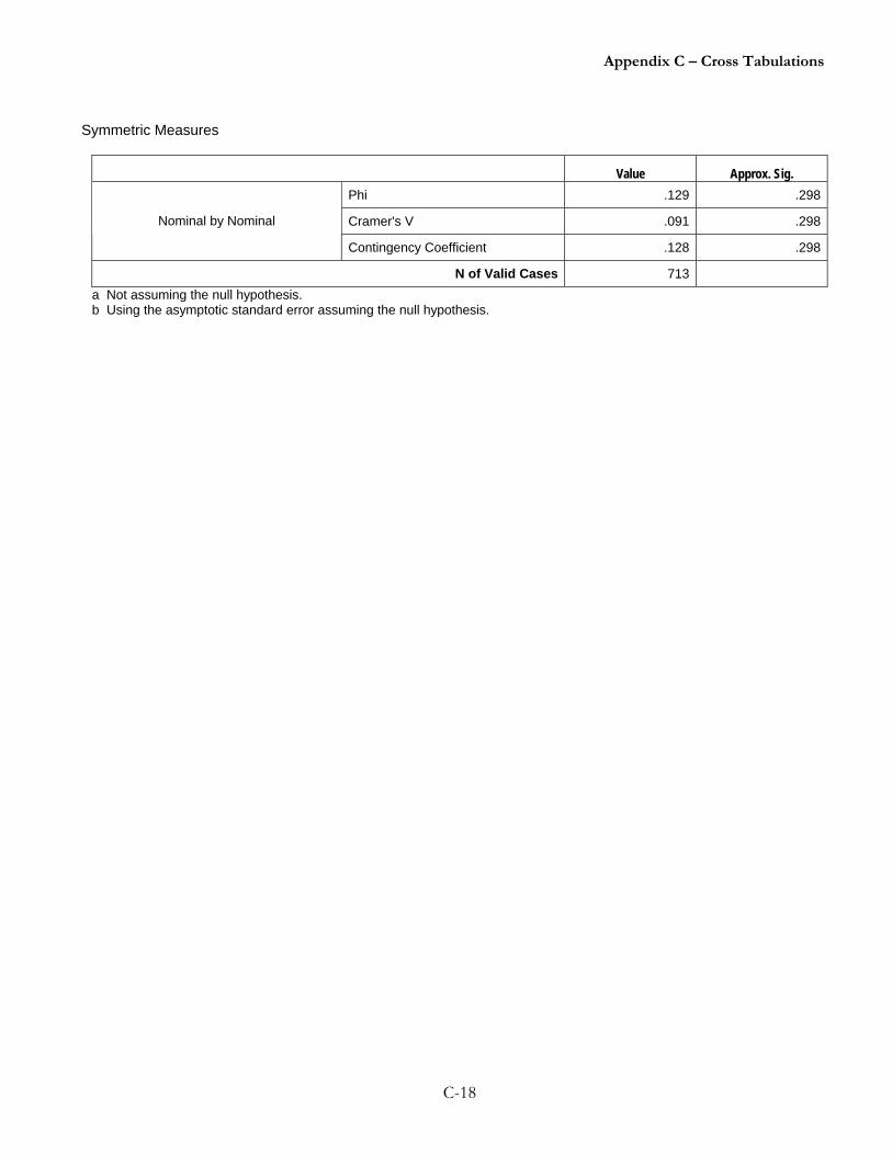
Appendix C – Cross Tabulations
C-18
Symmetric Measures
Value Approx. Sig. Phi .129 .298
Cramer's V .091 .298Nominal by Nominal
Contingency Coefficient .128 .298
N of Valid Cases 713 a Not assuming the null hypothesis. b Using the asymptotic standard error assuming the null hypothesis.

Appendix C – Cross Tabulations
C-19
II. Where Stormwater Goes 3. by Gender
Where would you say storm water runoff goes once it enters a storm drain? * Record gender of respondent. Crosstabulation Count
Record gender of respondent.
Female Male Total Where would you say storm water runoff goes once it enters a storm drain?
The city's regular sewer treatment plant 103 49 152
A separate special sewer treatment plant 38 15 53
Nearby fields and yards 45 25 70
Closest river, stream, or lake 131 137 268
Drainage pond 64 30 94
Refuse to answer 62 14 76
Total 443 270 713
Chi-Square Tests
Value df Asymp. Sig. (2-sided) Pearson Chi-Square 37.882(a) 5 .000
Likelihood Ratio 38.788 5 .000
Linear-by-Linear Association 2.091 1 .148
N of Valid Cases 713 a 0 cells (.0%) have expected count less than 5. The minimum expected count is 20.07.
Directional Measures
Value Where would you say storm water runoff goes once it enters a storm drain? Dependent .054
Nominal by Interval Eta Record gender of respondent. Dependent .230

Appendix C – Cross Tabulations
C-20
Symmetric Measures
Value Approx. Sig. Phi .230 .000
Cramer's V .230 .000Nominal by Nominal
Contingency Coefficient .225 .000
N of Valid Cases 713 a Not assuming the null hypothesis. b Using the asymptotic standard error assuming the null hypothesis.
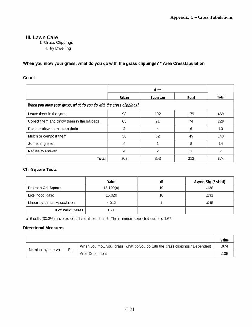
Appendix C – Cross Tabulations
C-21
III. Lawn Care 1. Grass Clippings a. by Dwelling
When you mow your grass, what do you do with the grass clippings? * Area Crosstabulation Count
Area Urban Suburban Rural Total
When you mow your grass, what do you do with the grass clippings?
Leave them in the yard 98 192 179 469
Collect them and throw them in the garbage 63 91 74 228
Rake or blow them into a drain 3 4 6 13
Mulch or compost them 36 62 45 143
Something else 4 2 8 14
Refuse to answer 4 2 1 7
Total 208 353 313 874
Chi-Square Tests
Value df Asymp. Sig. (2-sided) Pearson Chi-Square 15.120(a) 10 .128
Likelihood Ratio 15.020 10 .131
Linear-by-Linear Association 4.012 1 .045
N of Valid Cases 874
a 6 cells (33.3%) have expected count less than 5. The minimum expected count is 1.67. Directional Measures
Value When you mow your grass, what do you do with the grass clippings? Dependent .074
Nominal by Interval Eta Area Dependent .105

Appendix C – Cross Tabulations
C-22
Symmetric Measures
Value Approx. Sig. Phi .132 .128
Cramer's V .093 .128 Nominal by Nominal
Contingency Coefficient .130 .128
N of Valid Cases 874
a Not assuming the null hypothesis.
b Using the asymptotic standard error assuming the null hypothesis.

Appendix C – Cross Tabulations
C-23
III. Lawn Care 1. Grass Clippings b. by Education
When you mow your grass, what do you do with the grass clippings? * Area Crosstabulation Count
Which of the following categories would you say best describes your education level?
Less than high
school
Some high
school
High school
graduate
Some vocational
or technical school
Graduated from
vocational or technical
school Some
college
2-Year college
graduate
4-Year college gradua
te
Post-graduate degree Total
When you mow your grass, what do you do with the grass clippings?
Leave them in the yard 17 47 117 53 35 67 26 76 26 464
Collect them and throw them in the garbage 12 35 52 33 19 35 9 25 7 227
Rake or blow them into a drain 1 2 3 0 0 3 2 2 0 13
Mulch or compost them 2 12 19 7 6 23 16 30 26 141
Something else 1 1 3 0 0 3 0 2 4 14
Refuse to answer 1 0 1 0 0 2 0 1 2 7
Total 34 97 195 93 60 133 53 136 65 866
Chi-Square Tests
Value df Asymp. Sig. (2-sided) Pearson Chi-Square 98.663(a) 40 .000
Likelihood Ratio 97.350 40 .000
Linear-by-Linear Association 23.445 1 .000
N of Valid Cases 866 a 27 cells (50.0%) have expected count less than 5. The minimum expected count is .27.

Appendix C – Cross Tabulations
C-24
Directional Measures
Value When you mow your grass, what do you do with the grass clippings? Dependent .235
Nominal by Interval Eta Which of the following categories would you say best describes your education level? Dependent .240
Symmetric Measures
Value Approx. Sig. Phi .338 .000
Cramer's V .151 .000Nominal by Nominal
Contingency Coefficient .320 .000
N of Valid Cases 866 a Not assuming the null hypothesis. b Using the asymptotic standard error assuming the null hypothesis.

Appendix C – Cross Tabulations
C-25
III. Lawn Care 2. Fertilizer Use a. by Dwelling
About how often would you say you use fertilizer on your lawn? * Area Crosstabulation Count
Area Urban Suburban Rural Total
About how often would you say you use fertilizer on your lawn?
Monthly 9 8 4 21
Two or three times a year 50 72 45 167
Once a year or less 36 69 63 168
Refuse to answer 2 3 1 6
Total 97 152 113 362
Chi-Square Tests
Value df Asymp. Sig. (2-sided) Pearson Chi-Square 9.295(a) 6 .158
Likelihood Ratio 9.247 6 .160
Linear-by-Linear Association 1.244 1 .265
N of Valid Cases 362
a 3 cells (25.0%) have expected count less than 5. The minimum expected count is 1.61.

Appendix C – Cross Tabulations
C-26
Directional Measures
Value About how often would you say you use fertilizer on your lawn? Dependent .061
Nominal by Interval Eta Area Dependent .157
Symmetric Measures
Value Approx. Sig. Phi .160 .158
Cramer's V .113 .158Nominal by Nominal
Contingency Coefficient .158 .158
N of Valid Cases 362
a Not assuming the null hypothesis.
b Using the asymptotic standard error assuming the null hypothesis.

Appendix C – Cross Tabulations
C-27
III. Lawn Care 2. Fertilizer Use b. by Income
About how often would you say you use fertilizer on your lawn? * Which of the following categories best describes your annual household income before taxes? Crosstabulation Count
Which of the following categories best describes your annual household income before taxes?
Less than $12,000
$12,000 to $25,000
$25,000 to $35,000
$35,000 to $50,000
$50,000 to $75,000
$75,000 to $100,000
Over $100,000
Don't know
Refuse to
answer Total
About how often would you say you use fertilizer on your lawn?
Monthly 0 2 2 0 1 1 5 2 0 13
Two or three times a year 3 3 8 15 22 10 20 17 5 103
Once a year or less 9 18 20 25 31 22 10 26 7 168
Refuse to answer 1 1 0 0 0 0 0 2 0 4
Total 13 24 30 40 54 33 35 47 12 288
Chi-Square Tests
Value df Asymp. Sig. (2-sided) Pearson Chi-Square 40.962(a) 24 .017
Likelihood Ratio 42.453 24 .011
Linear-by-Linear Association 3.347 1 .067
N of Valid Cases 288
a 20 cells (55.6%) have expected count less than 5. The minimum expected count is .17. Directional Measures
Value About how often would you say you use fertilizer on your lawn? Dependent .259
Nominal by Interval Eta Which of the following categories best describes your annual household income before taxes? Dependent .159

Appendix C – Cross Tabulations
C-28
Symmetric Measures
Value Approx. Sig. Phi .377 .017
Cramer's V .218 .017 Nominal by Nominal
Contingency Coefficient .353 .017
N of Valid Cases 288
a Not assuming the null hypothesis.
b Using the asymptotic standard error assuming the null hypothesis.

Appendix C – Cross Tabulations
C-29
III. Lawn Care 2. Fertilizer Use c. by Age
About how often would you say you use fertilizer on your lawn? * Which of these categories best describes your age? Crosstabulation Count
Which of these categories best describes your age?
18-24 25-34 35-44 45-54 55-64 Over 65 Don't know Total
About how often would you say you use fertilizer on your lawn Monthly 1 1 12 1 2 3 1 21Two or three times a year 22 7 64 29 17 27 1 167Once a year or less 3 14 23 36 42 46 4 168Refuse to answer 0 0 2 1 0 2 1 6
Total 26 22 101 67 61 78 7 362
Chi-Square Tests
Value df Asymp. Sig. (2-sided) Pearson Chi-Square 74.602(a) 18 .000
Likelihood Ratio 75.353 18 .000
Linear-by-Linear Association 16.321 1 .000
N of Valid Cases 362 a 15 cells (53.6%) have expected count less than 5. The minimum expected count is .12.
Directional Measures
Value About how often would you say you use fertilizer on your lawn? Dependent .249
Nominal by Interval Eta Which of these categories best describes your age? Dependent .302

Appendix C – Cross Tabulations
C-30
Symmetric Measures
Value Approx. Sig. Nominal by Nominal Phi .454 .000
Cramer's V .262 .000
Contingency Coefficient .413 .000N of Valid Cases 362
a Not assuming the null hypothesis. b Using the asymptotic standard error assuming the null hypothesis.

Appendix C – Cross Tabulations
C-31
III. Lawn Care 3. Soil Test a. by Area
Does anyone ever test the soil on your lawn to determine how much fertilizer is needed? * Area Crosstabulation Count
Area Urban Suburban Rural Total
Does anyone ever test the soil on your lawn to determine how much fertilizer is needed?
Yes 50 63 48 161
No 45 89 64 198
Refuse to answer 2 2 2 6
Total 97 154 114 365 Chi-Square Tests
Value df Asymp. Sig. (2-sided) Pearson Chi-Square 3.436(a) 4 .488
Likelihood Ratio 3.434 4 .488
Linear-by-Linear Association .237 1 .627
N of Valid Cases 365 a 3 cells (33.3%) have expected count less than 5. The minimum expected count is 1.59. Directional Measures
Value Does anyone ever test the soil on your lawn to determine how much fertilizer is needed? Dependent .027
Nominal by Interval Eta Area Dependent .071

Appendix C – Cross Tabulations
C-32
Symmetric Measures
Value Approx. Sig. Phi .097 .488
Cramer's V .069 .488Nominal by Nominal
Contingency Coefficient .097 .488
N of Valid Cases 365 a Not assuming the null hypothesis. b Using the asymptotic standard error assuming the null hypothesis.

Appendix C – Cross Tabulations
C-33
III. Lawn Care 3. Soil Test b. by Age
Does anyone ever test the soil on your lawn to determine how much fertilizer is needed? * Which of these categories best describes your age? Crosstabulation
Count
Which of these categories best describes your age? 18-24 25-34 35-44 45-54 55-64 Over 65 Don't know Total
Does anyone ever test the soil on your lawn to determine how much fertilizer is needed?
Yes 20 6 66 26 20 20 3 161
No 6 15 36 43 41 55 2 198
Refuse to answer 0 1 0 0 0 3 2 6
Total 26 22 102 69 61 78 7 365
Chi-Square Tests
Value df Asymp. Sig. (2-sided) Pearson Chi-Square 84.142(a) 12 .000
Likelihood Ratio 65.126 12 .000
Linear-by-Linear Association 23.701 1 .000
N of Valid Cases 365
a 9 cells (42.9%) have expected count less than 5. The minimum expected count is .12. Directional Measures
Value Does anyone ever test the soil on your lawn to determine how much fertilizer is needed? Dependent .357
Nominal by Interval Eta Which of these categories best describes your age? Dependent .294

Appendix C – Cross Tabulations
C-34
Symmetric Measures
Value Approx. Sig.
Phi .480 .000
Cramer's V .340 .000Nominal by Nominal
Contingency Coefficient .433 .000
N of Valid Cases 365
a Not assuming the null hypothesis.
b Using the asymptotic standard error assuming the null hypothesis.

Appendix C – Cross Tabulations
C-35
III. Lawn Care 3. Soil Test c. by Gender
Does anyone ever test the soil on your lawn to determine how much fertilizer is needed? * Record gender of respondent.Crosstabulation Count
Record gender of respondent. Female Male Total
Does anyone ever test the soil on your lawn to determine how much fertilizer is needed?
Yes 97 64 161
No 121 77 198
Refuse to answer 6 0 6
Total 224 141 365
Chi-Square Tests
Value df Asymp. Sig. (2-sided) Pearson Chi-Square 3.868(a) 2 .145
Likelihood Ratio 5.950 2 .051
Linear-by-Linear Association 3.286 1 .070
N of Valid Cases 365
a 2 cells (33.3%) have expected count less than 5. The minimum expected count is 2.32. Directional Measures
Value Does anyone ever test the soil on your lawn to determine how much fertilizer is needed? Dependent .095
Nominal by Interval Eta Record gender of respondent. Dependent .103

Appendix C – Cross Tabulations
C-36
Symmetric Measures
Value Approx. Sig. Phi .103 .145
Cramer's V .103 .145 Nominal by Nominal
Contingency Coefficient .102 .145
N of Valid Cases 365
a Not assuming the null hypothesis.
b Using the asymptotic standard error assuming the null hypothesis.

Appendix C – Cross Tabulations
C-37
IV. Vehicle Care 1. Washing a. by Dwelling
When you wash your vehicle at home, does the soapy water flow into the grass, or onto the street? * Area Crosstabulation Count
Area
Urban Suburban Rural Total
When you wash your vehicle at home, does the soapy water flow into the grass, or onto the street?
Into the grass, dirt or gravel 34 69 85 188
Into the street or driveway 36 54 38 128
Varies, sometimes one, sometimes another 1 9 4 14
Don't know 0 0 1 1
Total 71 132 128 331
Chi-Square Tests
Value df Asymp. Sig. (2-sided) Pearson Chi-Square 14.432(a) 6 .025
Likelihood Ratio 14.877 6 .021
Linear-by-Linear Association 1.951 1 .162
N of Valid Cases 331
a 4 cells (33.3%) have expected count less than 5. The minimum expected count is .21. Directional Measures
Value When you wash your vehicle at home, does the soapy water flow into the grass, or onto the street? Dependent .092
Nominal by Interval Eta Area Dependent .173

Appendix C – Cross Tabulations
C-38
Symmetric Measures
Value Approx. Sig. Phi .209 .025
Cramer's V .148 .025 Nominal by Nominal
Contingency Coefficient .204 .025
N of Valid Cases 331
a Not assuming the null hypothesis.
b Using the asymptotic standard error assuming the null hypothesis.
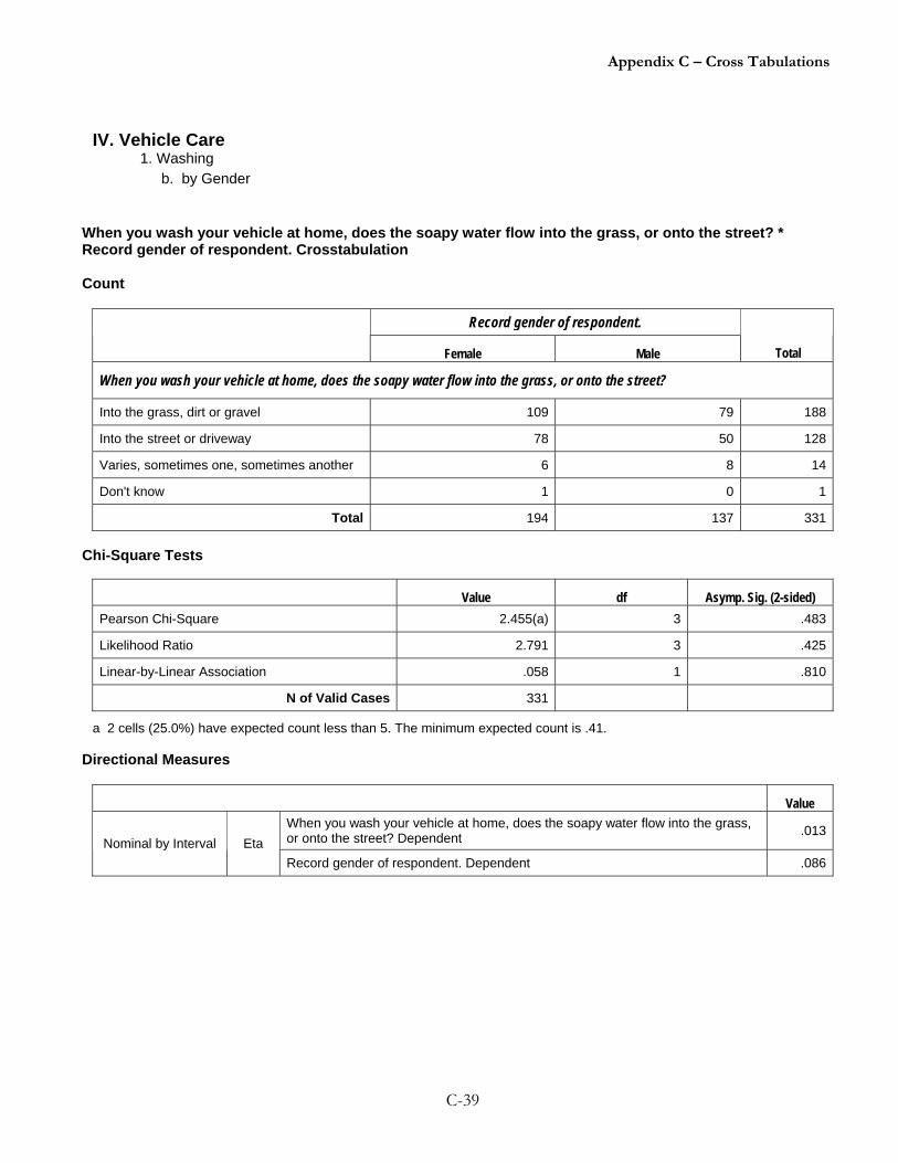
Appendix C – Cross Tabulations
C-39
IV. Vehicle Care 1. Washing b. by Gender
When you wash your vehicle at home, does the soapy water flow into the grass, or onto the street? * Record gender of respondent. Crosstabulation Count
Record gender of respondent.
Female Male Total
When you wash your vehicle at home, does the soapy water flow into the grass, or onto the street?
Into the grass, dirt or gravel 109 79 188
Into the street or driveway 78 50 128
Varies, sometimes one, sometimes another 6 8 14
Don't know 1 0 1
Total 194 137 331
Chi-Square Tests
Value df Asymp. Sig. (2-sided) Pearson Chi-Square 2.455(a) 3 .483
Likelihood Ratio 2.791 3 .425
Linear-by-Linear Association .058 1 .810
N of Valid Cases 331
a 2 cells (25.0%) have expected count less than 5. The minimum expected count is .41.
Directional Measures
Value When you wash your vehicle at home, does the soapy water flow into the grass, or onto the street? Dependent .013
Nominal by Interval Eta Record gender of respondent. Dependent .086

Appendix C – Cross Tabulations
C-40
Symmetric Measures
Value Approx. Sig. Phi .086 .483
Cramer's V .086 .483Nominal by Nominal
Contingency Coefficient .086 .483
N of Valid Cases 331
a Not assuming the null hypothesis.
b Using the asymptotic standard error assuming the null hypothesis.

Appendix C – Cross Tabulations
C-41
IV. Vehicle Care 1. Washing c. by Age
When you wash your vehicle at home, does the soapy water flow into the grass, or onto the street? * Which of these categories best describes your age? Crosstabulation Count
Which of these categories best describes your age? 18-24 25-34 35-44 45-54 55-64 Over 65 Don't know Total
When you wash your vehicle at home, does the soapy water flow into the grass, or onto the street?
Into the grass, dirt or gravel 17 15 47 35 32 41 1 188
Into the street or driveway 15 5 52 19 19 15 3 128
sometimes one, sometimes another 1 2 5 4 1 1 0 14
Don't know 0 1 0 0 0 0 0 1
Total 33 23 104 58 52 57 4 331
Chi-Square Tests
Value df Asymp. Sig. (2-sided) Pearson Chi-Square 33.304(a) 18 .015
Likelihood Ratio 25.624 18 .109
Linear-by-Linear Association 5.315 1 .021
N of Valid Cases 331
a 16 cells (57.1%) have expected count less than 5. The minimum expected count is .01.
Directional Measures
Value When you wash your vehicle at home, does the soapy water flow into the grass, or onto the street? Dependent .180
Nominal by Interval Eta Which of these categories best describes your age? Dependent .127

Appendix C – Cross Tabulations
C-42
Symmetric Measures
Value Approx. Sig. Phi .317 .015
Cramer's V .183 .015Nominal by Nominal
Contingency Coefficient .302 .015
N of Valid Cases 331
a Not assuming the null hypothesis.
b Using the asymptotic standard error assuming the null hypothesis.
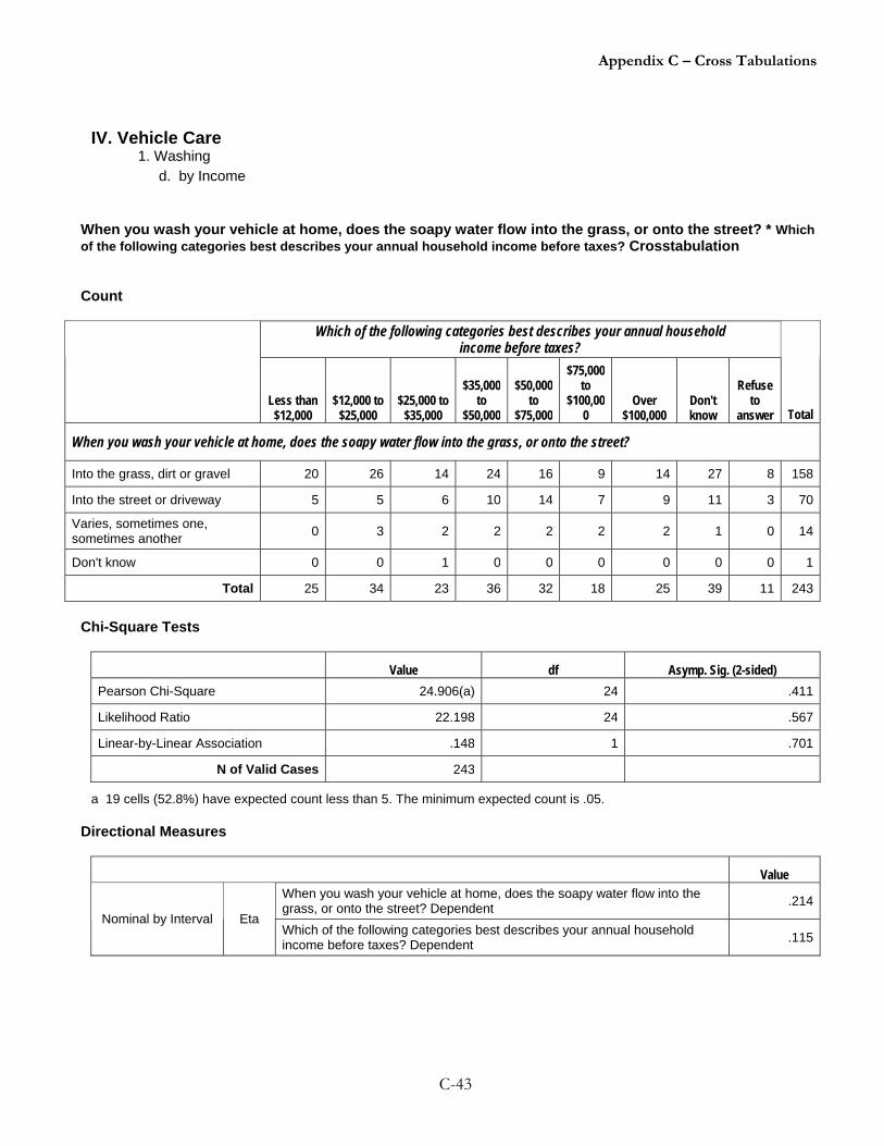
Appendix C – Cross Tabulations
C-43
IV. Vehicle Care 1. Washing d. by Income
When you wash your vehicle at home, does the soapy water flow into the grass, or onto the street? * Which of the following categories best describes your annual household income before taxes? Crosstabulation Count
Which of the following categories best describes your annual household income before taxes?
Less than $12,000
$12,000 to $25,000
$25,000 to $35,000
$35,000 to
$50,000
$50,000 to
$75,000
$75,000 to
$100,000
Over $100,000
Don't know
Refuse to
answer
Total
When you wash your vehicle at home, does the soapy water flow into the grass, or onto the street?
Into the grass, dirt or gravel 20 26 14 24 16 9 14 27 8 158
Into the street or driveway 5 5 6 10 14 7 9 11 3 70
Varies, sometimes one, sometimes another 0 3 2 2 2 2 2 1 0 14
Don't know 0 0 1 0 0 0 0 0 0 1
Total 25 34 23 36 32 18 25 39 11 243
Chi-Square Tests
Value df Asymp. Sig. (2-sided) Pearson Chi-Square 24.906(a) 24 .411
Likelihood Ratio 22.198 24 .567
Linear-by-Linear Association .148 1 .701
N of Valid Cases 243
a 19 cells (52.8%) have expected count less than 5. The minimum expected count is .05. Directional Measures
Value When you wash your vehicle at home, does the soapy water flow into the grass, or onto the street? Dependent .214
Nominal by Interval Eta Which of the following categories best describes your annual household income before taxes? Dependent .115

Appendix C – Cross Tabulations
C-44
Symmetric Measures
Value Approx. Sig. Phi .320 .411
Cramer's V .185 .411 Nominal by Nominal
Contingency Coefficient .305 .411
N of Valid Cases 243
a Not assuming the null hypothesis.
b Using the asymptotic standard error assuming the null hypothesis.

Appendix C – Cross Tabulations
C-45
IV. Vehicle Care 2. Oil Change a. by Dwelling
When you change your oil at home, how do you dispose of the used oil? * Area Crosstabulation Count
Area
Urban Suburban Rural Total
When you change your oil at home, how do you dispose of the used oil?
In a designated lawn area 2 10 10 22
With other garbage (dumpster, placed in trash bags, etc) 7 14 15 36
Pour it down a storm drain 3 6 7 16
Take it somewhere it can be recycled 15 44 32 91
Other 0 2 8 10
Refuse to answer 2 1 1 4
Total 29 77 73 179
Chi-Square Tests
Value df Asymp. Sig. (2-sided) Pearson Chi-Square 12.730(a) 10 .239
Likelihood Ratio 13.030 10 .222
Linear-by-Linear Association .565 1 .452
N of Valid Cases 179
a 8 cells (44.4%) have expected count less than 5. The minimum expected count is .65.
Directional Measures
Value When you change your oil at home, how do you dispose of the used oil? Dependent .074
Nominal by Interval Eta Area Dependent .227
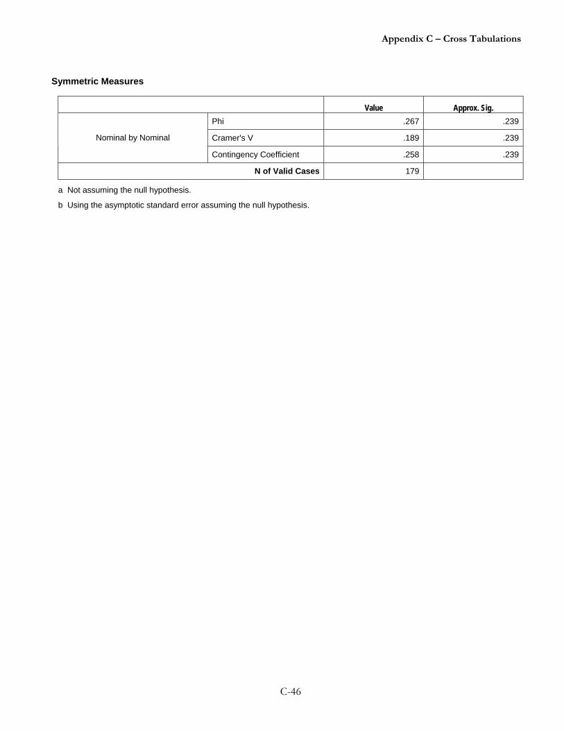
Appendix C – Cross Tabulations
C-46
Symmetric Measures
Value Approx. Sig. Phi .267 .239
Cramer's V .189 .239Nominal by Nominal
Contingency Coefficient .258 .239
N of Valid Cases 179
a Not assuming the null hypothesis.
b Using the asymptotic standard error assuming the null hypothesis.

Appendix C – Cross Tabulations
C-47
IV. Vehicle Care 2. Oil Change b. by Race
When you change your oil at home, how do you dispose of the used oil? * How would you classify yourself? Crosstabulation Count
How would you classify yourself?
Black or African-
American Asian White Hispanic Other Don't know
Refuse to answer Total
When you change your oil at home, how do you dispose of the used oil?
In a designated lawn area 2 0 9 2 3 6 0 22
With other garbage (dumpster, placed in trash bags, etc) 4 3 15 4 3 5 1 35
Pour it down a storm drain 2 4 2 3 2 2 0 15
Take it somewhere it can be recycled 6 1 72 4 6 2 0 91
Other 1 0 8 1 0 0 0 10
Refuse to answer 3 1 0 0 0 0 0 4
Total 18 9 106 14 14 15 1 177
Chi-Square Tests
Value df Asymp. Sig. (2-sided) Pearson Chi-Square 85.618(a) 30 .000
Likelihood Ratio 74.064 30 .000
Linear-by-Linear Association 20.716 1 .000
N of Valid Cases 177
a 33 cells (78.6%) have expected count less than 5. The minimum expected count is .02.
Directional Measures
Value When you change your oil at home, how do you dispose of the used oil? Dependent .354
Nominal by Interval Eta How would you classify yourself? Dependent .347

Appendix C – Cross Tabulations
C-48
Symmetric Measures
Value Approx. Sig. Phi .695 .000
Cramer's V .311 .000Nominal by Nominal
Contingency Coefficient .571 .000
N of Valid Cases 177
a Not assuming the null hypothesis. b Using the asymptotic standard error assuming the null hypothesis.

Appendix C – Cross Tabulations
C-49
IV. Vehicle Care 2. Oil Change c. by Age
When you change your oil at home, how do you dispose of the used oil? * Which of these categories best describes your age? Crosstabulation Count
Which of these categories best describes your age?
18-24 25-34 35-44 45-54 55-64 Over 65 Don't know Total
When you change your oil at home, how do you dispose of the used oil?
In a designated lawn area 5 1 12 2 1 1 0 22
With other garbage (dumpster, placed in trash bags, etc) 7 1 15 8 3 2 0 36
Pour it down a storm drain 2 2 7 4 1 0 0 16
Take it somewhere it can be recycled 5 12 22 23 14 13 2 91
Other 1 0 2 4 0 3 0 10
Refuse to answer 1 1 0 1 0 1 0 4
Total 21 17 58 42 19 20 2 179
Chi-Square Tests
Value df Asymp. Sig. (2-sided) Pearson Chi-Square 40.218(a) 30 .101
Likelihood Ratio 45.841 30 .032
Linear-by-Linear Association 7.596 1 .006
N of Valid Cases 179
a 31 cells (73.8%) have expected count less than 5. The minimum expected count is .04. Directional Measures
Value When you change your oil at home, how do you dispose of the used oil? Dependent .336
Nominal by Interval Eta Which of these categories best describes your age? Dependent .292

Appendix C – Cross Tabulations
C-50
Symmetric Measures
Value Approx. Sig. Phi .474 .101
Cramer's V .212 .101Nominal by Nominal
Contingency Coefficient .428 .101
N of Valid Cases 179
a Not assuming the null hypothesis.
b Using the asymptotic standard error assuming the null hypothesis.

Appendix C – Cross Tabulations
C-51
V. Pet Waste Disposal 1. by Dwelling
How often do you pick up their pet waste? * Area Crosstabulation Count
Area
Urban Suburban Rural Total
How often do you pick up their pet waste?
Always 48 63 41 152
Often 5 14 12 31
Sometimes 23 26 19 68
Rarely 45 45 55 145
Never 25 67 64 156
Refuse to answer 2 10 7 19
Total 148 225 198 571
Chi-Square Tests
Value df Asymp. Sig. (2-sided) Pearson Chi-Square 24.038(a) 10 .008
Likelihood Ratio 25.562 10 .004
Linear-by-Linear Association 9.107 1 .003
N of Valid Cases 571
a 1 cells (5.6%) have expected count less than 5. The minimum expected count is 4.92. Directional Measures
Value How often do you pick up their pet waste? Dependent .129
Nominal by Interval Eta Area Dependent .167

Appendix C – Cross Tabulations
C-52
Symmetric Measures
Value Approx. Sig. Phi .205 .008
Cramer's V .145 .008 Nominal by Nominal
Contingency Coefficient .201 .008
N of Valid Cases 571
a Not assuming the null hypothesis.
b Using the asymptotic standard error assuming the null hypothesis.
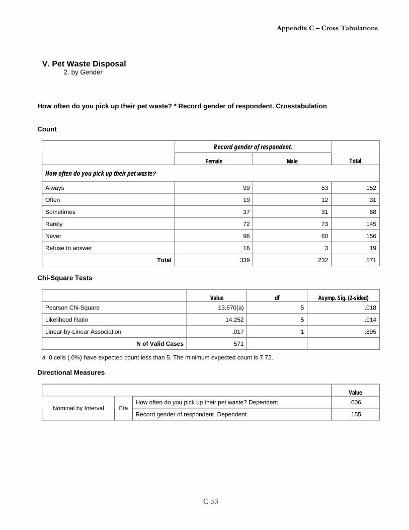
Appendix C – Cross Tabulations
C-53
V. Pet Waste Disposal 2. by Gender
How often do you pick up their pet waste? * Record gender of respondent. Crosstabulation Count
Record gender of respondent.
Female Male Total
How often do you pick up their pet waste?
Always 99 53 152
Often 19 12 31
Sometimes 37 31 68
Rarely 72 73 145
Never 96 60 156
Refuse to answer 16 3 19
Total 339 232 571
Chi-Square Tests
Value df Asymp. Sig. (2-sided) Pearson Chi-Square 13.670(a) 5 .018
Likelihood Ratio 14.252 5 .014
Linear-by-Linear Association .017 1 .895
N of Valid Cases 571
a 0 cells (.0%) have expected count less than 5. The minimum expected count is 7.72. Directional Measures
Value How often do you pick up their pet waste? Dependent .006
Nominal by Interval Eta Record gender of respondent. Dependent .155

Appendix C – Cross Tabulations
C-54
Symmetric Measures
Value Approx. Sig. Phi .155 .018
Cramer's V .155 .018Nominal by Nominal
Contingency Coefficient .153 .018
N of Valid Cases 571
a Not assuming the null hypothesis.
b Using the asymptotic standard error assuming the null hypothesis.

Appendix C – Cross Tabulations
C-55
V. Pet Waste Disposal 3. by Age
How often do you pick up their pet waste? * Which of these categories best describes your age? Crosstabulation Count
Which of these categories best describes your age?
18-24 25-34 35-44 45-54 55-64 Over 65 Don't know Total
How often do you pick up their pet waste?
Always 24 8 58 24 16 19 3 152
Often 3 2 18 3 3 1 1 31
Sometimes 14 5 20 14 6 8 1 68
Rarely 19 2 86 19 13 2 4 145
Never 16 16 46 36 27 15 0 156
Refuse to answer 4 0 13 2 0 0 0 19
Total 80 33 241 98 65 45 9 571
Chi-Square Tests
Value df Asymp. Sig. (2-sided) Pearson Chi-Square 77.000(a) 30 .000
Likelihood Ratio 87.337 30 .000
Linear-by-Linear Association 1.204 1 .273
N of Valid Cases 571
a 16 cells (38.1%) have expected count less than 5. The minimum expected count is .30. Directional Measures
Value How often do you pick up their pet waste? Dependent .111
Nominal by Interval Eta Which of these categories best describes your age? Dependent .126

Appendix C – Cross Tabulations
C-56
Symmetric Measures
Value Approx. Sig. Phi .367 .000
Cramer's V .164 .000 Nominal by Nominal
Contingency Coefficient .345 .000
N of Valid Cases 571
a Not assuming the null hypothesis.
b Using the asymptotic standard error assuming the null hypothesis.