Embed Size (px)
Citation preview
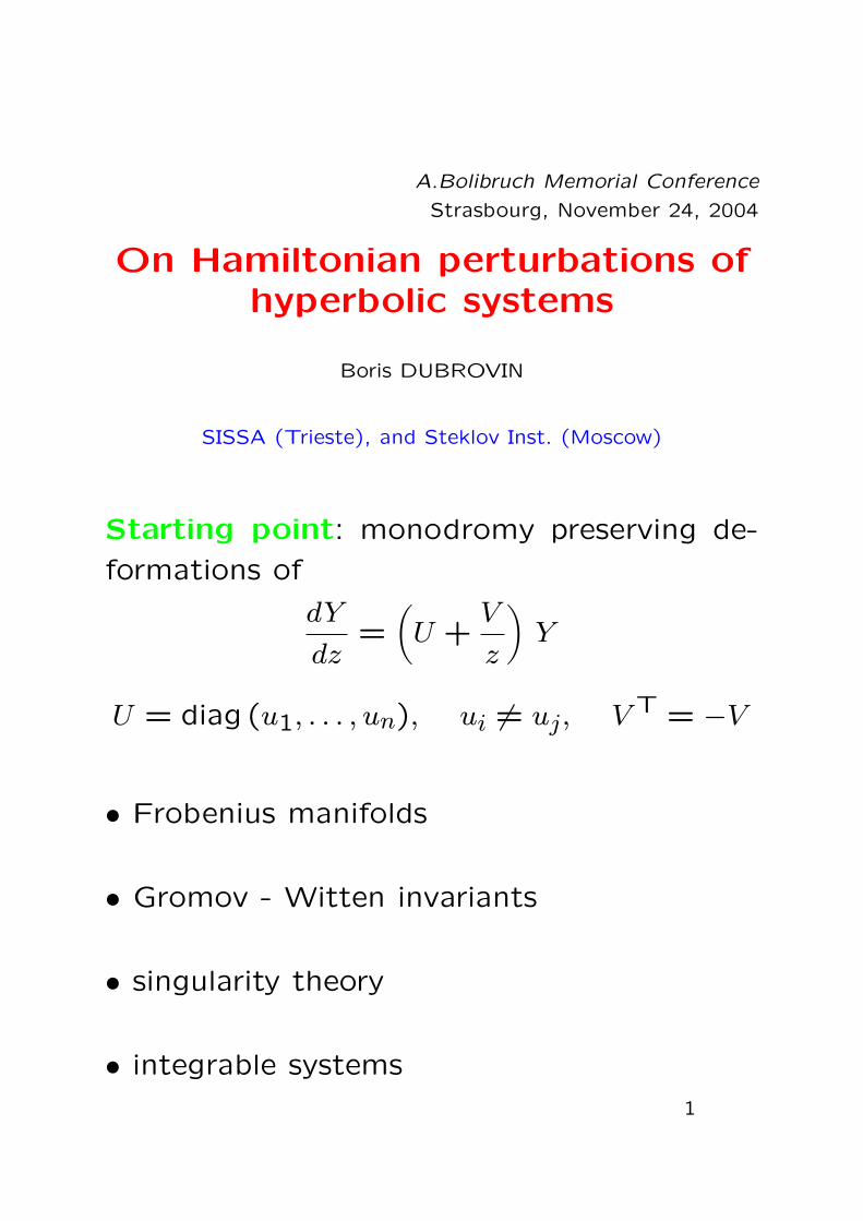
A.Bolibruch Memorial Conference
Strasbourg, November 24, 2004
On Hamiltonian perturbations ofhyperbolic systems
Boris DUBROVIN
SISSA (Trieste), and Steklov Inst. (Moscow)
Starting point: monodromy preserving de-
formations of
dY
dz=(U +
V
z
)Y
U = diag (u1, . . . , un), ui 6= uj, V T = −V
• Frobenius manifolds
• Gromov - Witten invariants
• singularity theory
• integrable systems
1
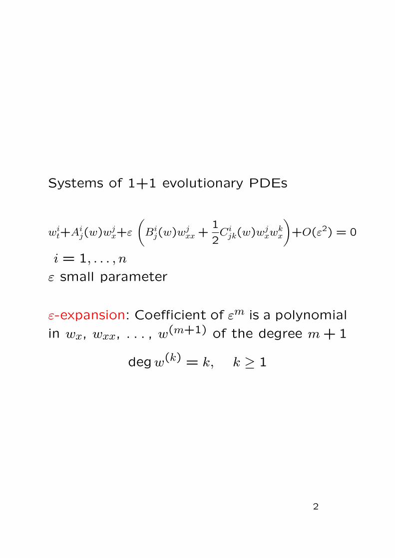
Systems of 1+1 evolutionary PDEs
wit+Aij(w)wjx+ε
(Bij(w)wjxx +
1
2Cijk(w)wjxw
kx
)+O(ε2) = 0
i = 1, . . . , n
ε small parameter
ε-expansion: Coefficient of εm is a polynomial
in wx, wxx, . . . , w(m+1) of the degree m+ 1
degw(k) = k, k ≥ 1
2
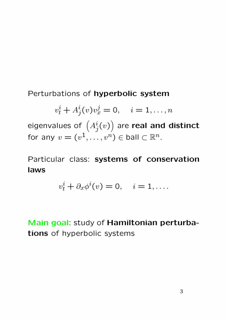
Perturbations of hyperbolic system
vit +Aij(v)vjx = 0, i = 1, . . . , n
eigenvalues of(Aij(v)
)are real and distinct
for any v = (v1, . . . , vn) ∈ ball ⊂ Rn.
Particular class: systems of conservation
laws
vit + ∂xφi(v) = 0, i = 1, . . . .
Main goal: study of Hamiltonian perturba-
tions of hyperbolic systems
3
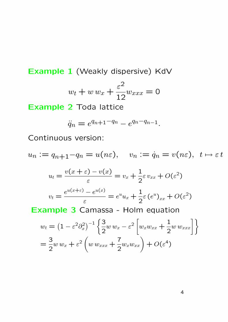
Example 1 (Weakly dispersive) KdV
wt + wwx +ε2
12wxxx = 0
Example 2 Toda lattice
qn = eqn+1−qn − eqn−qn−1.
Continuous version:
un := qn+1−qn = u(nε), vn := qn = v(nε), t 7→ ε t
ut =v(x+ ε)− v(x)
ε= vx +
1
2ε vxx +O(ε2)
vt =eu(x+ε) − eu(x)
ε= euux +
1
2ε (eu)xx +O(ε2)
Example 3 Camassa - Holm equation
wt =(1− ε2∂2
x
)−1{
3
2wwx − ε2
[wxwxx +
1
2wwxxx
]}=
3
2wwx + ε2
(wwxxx +
7
2wxwxx
)+O(ε4)
4
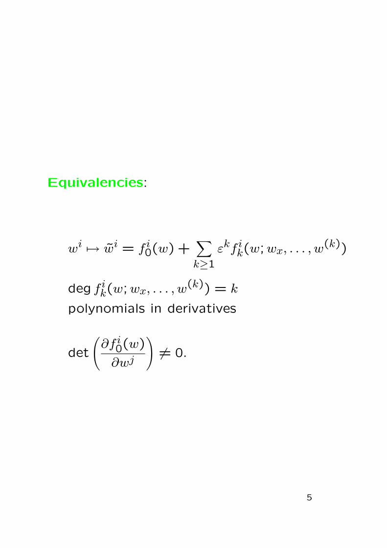
Equivalencies:
wi 7→ wi = f i0(w) +∑k≥1
εkf ik(w;wx, . . . , w(k))
deg f ik(w;wx, . . . , w(k)) = k
polynomials in derivatives
det
(∂f i0(w)
∂wj
)6= 0.
5

Questions:
structure of solutions for
• t < tc
• t ∼ tc
• t > tc
tc = time of gradient catastrophe for the
hyperbolic system
vit +Aij(v)vjx = 0
6
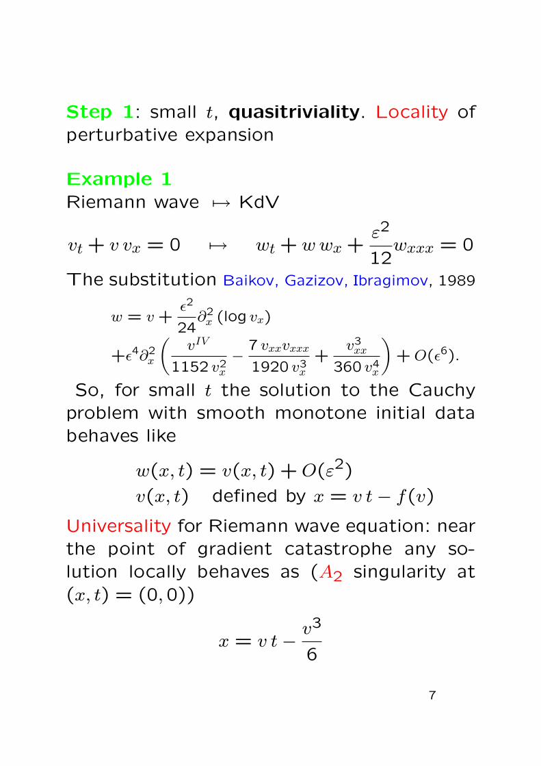
Step 1: small t, quasitriviality. Locality ofperturbative expansion
Example 1Riemann wave 7→ KdV
vt + v vx = 0 7→ wt + wwx +ε2
12wxxx = 0
The substitution Baikov, Gazizov, Ibragimov, 1989
w = v+ε2
24∂2x (log vx)
+ε4∂2x
(vIV
1152 v2x
−7 vxxvxxx1920 v3
x
+v3xx
360 v4x
)+O(ε6).
So, for small t the solution to the Cauchyproblem with smooth monotone initial databehaves like
w(x, t) = v(x, t) +O(ε2)
v(x, t) defined by x = v t− f(v)
Universality for Riemann wave equation: nearthe point of gradient catastrophe any so-lution locally behaves as (A2 singularity at(x, t) = (0,0))
x = v t−v3
6
7
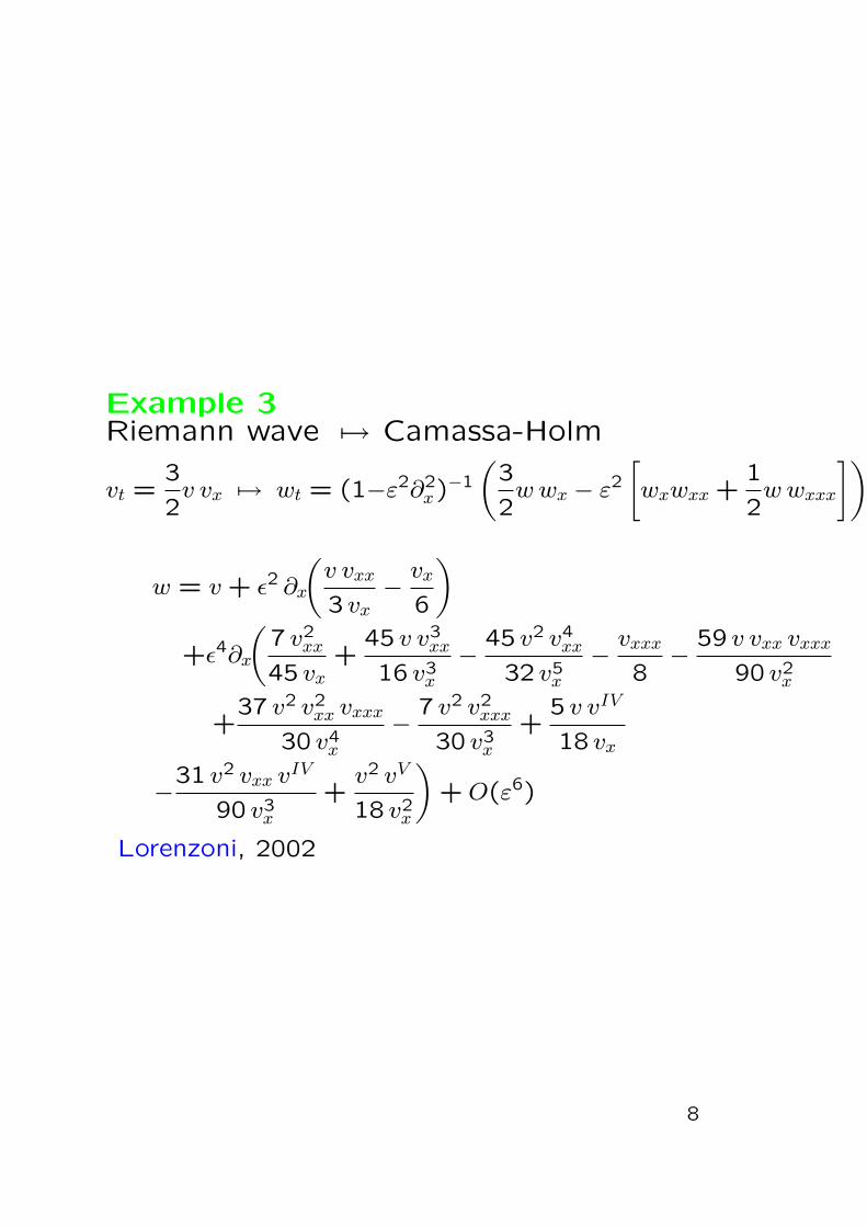
Example 3Riemann wave 7→ Camassa-Holm
vt =3
2v vx 7→ wt = (1−ε2∂2
x)−1
(3
2wwx − ε2
[wxwxx +
1
2wwxxx
])
w = v+ ε2 ∂x
(v vxx
3 vx−vx
6
)+ε4∂x
(7 v2
xx
45 vx+
45 v v3xx
16 v3x
−45 v2 v4
xx
32 v5x
−vxxx
8−
59 v vxx vxxx90 v2
x
+37 v2 v2
xx vxxx
30 v4x
−7 v2 v2
xxx
30 v3x
+5 v vIV
18 vx
−31 v2 vxx vIV
90 v3x
+v2 vV
18 v2x
)+O(ε6)
Lorenzoni, 2002
8
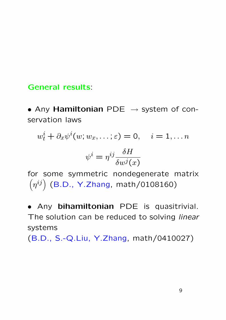
General results:
• Any Hamiltonian PDE → system of con-
servation laws
wit + ∂xψi(w;wx, . . . ; ε) = 0, i = 1, . . . n
ψi = ηijδH
δwj(x)
for some symmetric nondegenerate matrix(ηij)
(B.D., Y.Zhang, math/0108160)
• Any bihamiltonian PDE is quasitrivial.
The solution can be reduced to solving linear
systems
(B.D., S.-Q.Liu, Y.Zhang, math/0410027)
9

• Explicit construction: under assumptions of
existence of a tau-function and linear ac-
tion of the Virasoro symmetries onto the
tau-function
τ 7→ τ + δ Lmτ +O(δ2), m ≥ −1
via solving certain Riemann - Hilbert problem
(reconstructing the equation
dY
dz=(U +
V
z
)Y
starting from the “monodromy data”)
All solutions regular in ε obtained from the
vacuum solution
Lmτvac = 0, m ≥ −1
by shifts along the times of the hierarchy
(completeness needed!).
10
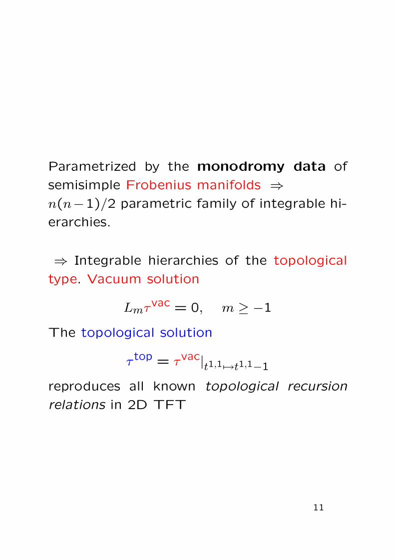
Parametrized by the monodromy data of
semisimple Frobenius manifolds ⇒n(n−1)/2 parametric family of integrable hi-
erarchies.
⇒ Integrable hierarchies of the topological
type. Vacuum solution
Lmτvac = 0, m ≥ −1
The topological solution
τ top = τvac|t1,1 7→t1,1−1
reproduces all known topological recursion
relations in 2D TFT
11
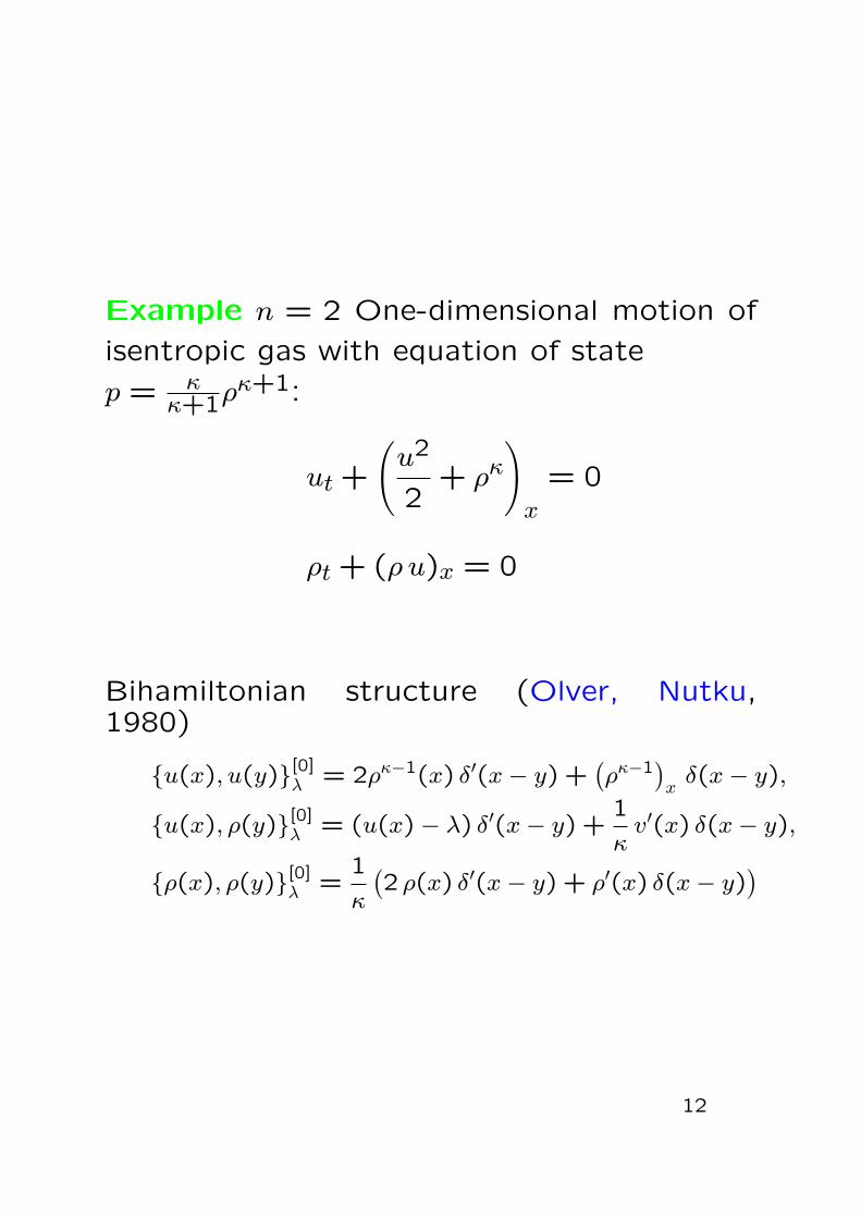
Example n = 2 One-dimensional motion of
isentropic gas with equation of state
p = κκ+1ρ
κ+1:
ut +
(u2
2+ ρκ
)x
= 0
ρt + (ρ u)x = 0
Bihamiltonian structure (Olver, Nutku,1980)
{u(x), u(y)}[0]λ = 2ρκ−1(x) δ′(x− y) +
(ρκ−1
)xδ(x− y),
{u(x), ρ(y)}[0]λ = (u(x)− λ) δ′(x− y) +
1
κv′(x) δ(x− y),
{ρ(x), ρ(y)}[0]λ =
1
κ
(2 ρ(x) δ′(x− y) + ρ′(x) δ(x− y)
)
12
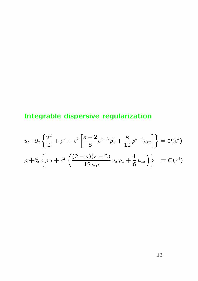
Integrable dispersive regularization
ut+∂x
{u2
2+ ρκ + ε2
[κ− 2
8ρκ−3 ρ2x +
κ
12ρκ−2ρxx
]}= O(ε4)
ρt+∂x
{ρ u+ ε2
((2− κ)(κ− 3)
12κ ρux ρx +
1
6uxx
)}= O(ε4)
13
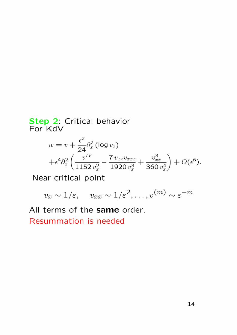
Step 2: Critical behaviorFor KdV
w = v+ε2
24∂2x (log vx)
+ε4∂2x
(vIV
1152 v2x
−7 vxxvxxx1920 v3
x
+v3xx
360 v4x
)+O(ε6).
Near critical point
vx ∼ 1/ε, vxx ∼ 1/ε2, . . . , v(m) ∼ ε−m
All terms of the same order.
Resummation is needed
14
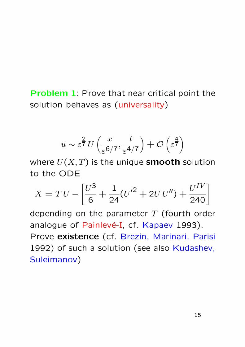
Problem 1: Prove that near critical point the
solution behaves as (universality)
u ∼ ε27 U
(x
ε6/7,t
ε4/7
)+O
(ε47
)where U(X,T ) is the unique smooth solution
to the ODE
X = T U −[U3
6+
1
24(U ′2 + 2U U ′′) +
UIV
240
]depending on the parameter T (fourth order
analogue of Painleve-I, cf. Kapaev 1993).
Prove existence (cf. Brezin, Marinari, Parisi
1992) of such a solution (see also Kudashev,
Suleimanov)
15
Step 3: After phase transition: oscillatory be-
havior. Gurevich, Pitaevski 1973, Whitham
asymptotics (leading term)
Problem 2 Determine full asymptotic behav-
ior of averaged quantities, ε→ 0
16
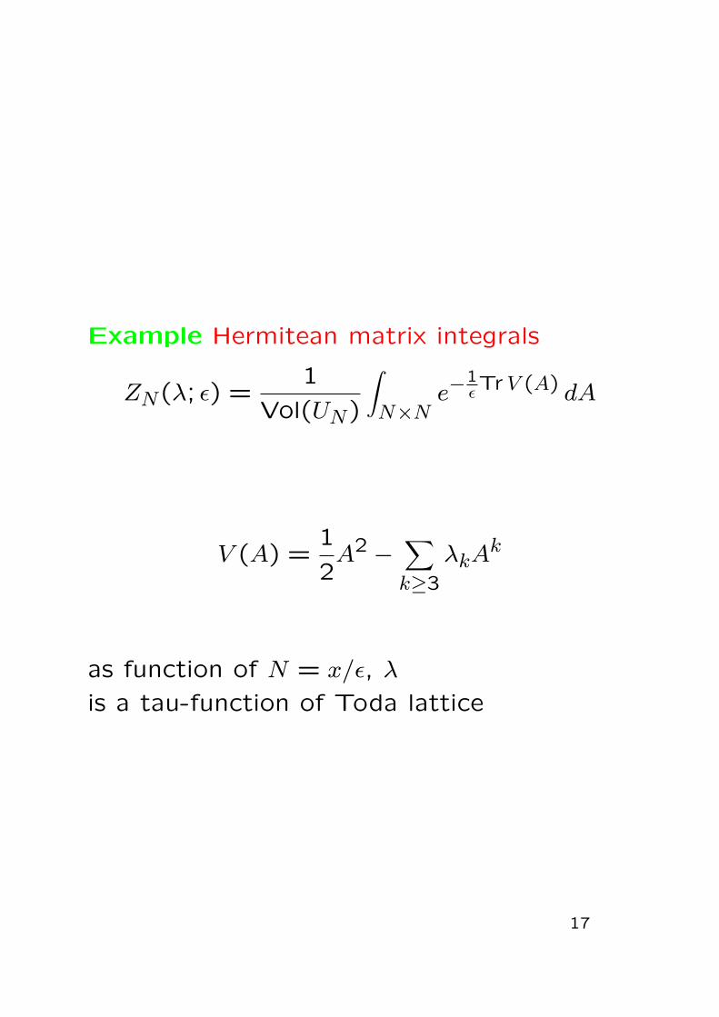
Example Hermitean matrix integrals
ZN(λ; ε) =1
Vol(UN)
∫N×N
e−1εTr V (A) dA
V (A) =1
2A2 −
∑k≥3
λkAk
as function of N = x/ε, λ
is a tau-function of Toda lattice
17
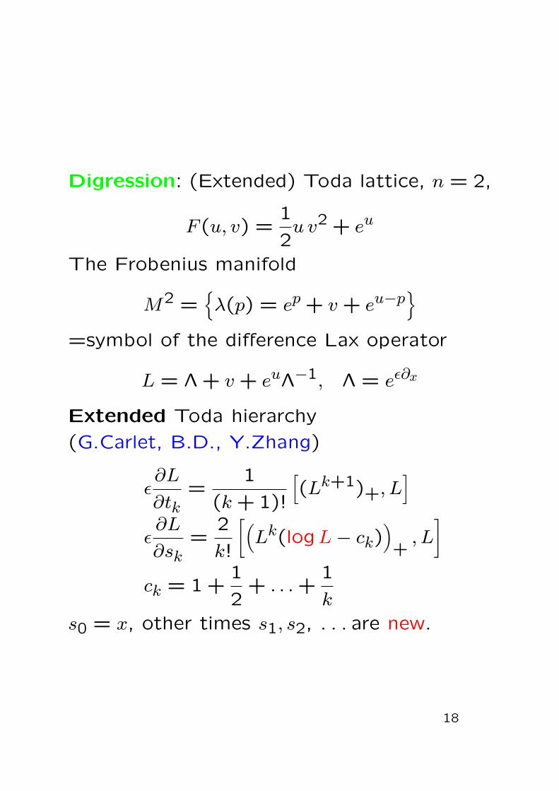
Digression: (Extended) Toda lattice, n = 2,
F (u, v) =1
2u v2 + eu
The Frobenius manifold
M2 ={λ(p) = ep + v+ eu−p
}=symbol of the difference Lax operator
L = Λ + v+ euΛ−1, Λ = eε∂x
Extended Toda hierarchy
(G.Carlet, B.D., Y.Zhang)
ε∂L
∂tk=
1
(k+ 1)!
[(Lk+1)+, L
]ε∂L
∂sk=
2
k!
[(Lk(logL− ck)
)+, L
]ck = 1 +
1
2+ . . .+
1
k
s0 = x, other times s1, s2, . . . are new.
18
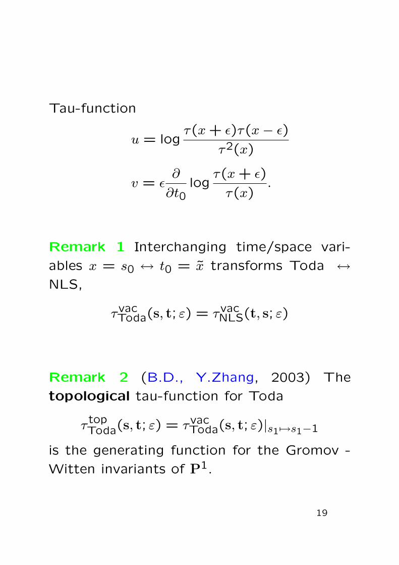
Tau-function
u = logτ(x+ ε)τ(x− ε)
τ2(x)
v = ε∂
∂t0log
τ(x+ ε)
τ(x).
Remark 1 Interchanging time/space vari-
ables x = s0 ↔ t0 = x transforms Toda ↔NLS,
τvacToda(s, t; ε) = τvacNLS(t, s; ε)
Remark 2 (B.D., Y.Zhang, 2003) The
topological tau-function for Toda
τ topToda(s, t; ε) = τvacToda(s, t; ε)|s1 7→s1−1
is the generating function for the Gromov -
Witten invariants of P1.
19

For small λ the ε-expansion can be obtained
by applying the saddle point method to
ZN =1
Vol(UN)
∫e−
1εTrV (A)dA
⇒ Fg(x, t) = generating function of numbers
of fat graphs on genus g Riemann surfaces
20
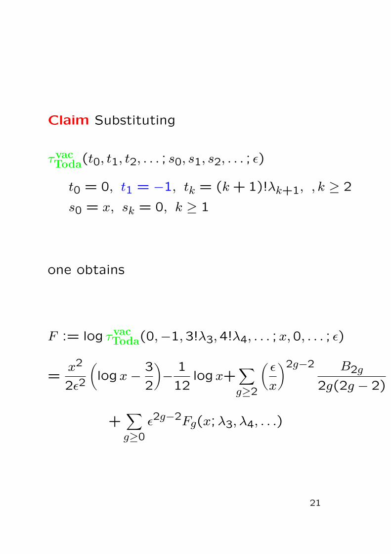
Claim Substituting
τvacToda(t0, t1, t2, . . . ; s0, s1, s2, . . . ; ε)
t0 = 0, t1 = −1, tk = (k+ 1)!λk+1, , k ≥ 2
s0 = x, sk = 0, k ≥ 1
one obtains
F := log τvacToda(0,−1,3!λ3,4!λ4, . . . ;x,0, . . . ; ε)
=x2
2ε2
(logx−
3
2
)−
1
12logx+
∑g≥2
(ε
x
)2g−2 B2g
2g(2g − 2)
+∑g≥0
ε2g−2Fg(x;λ3, λ4, . . .)
21
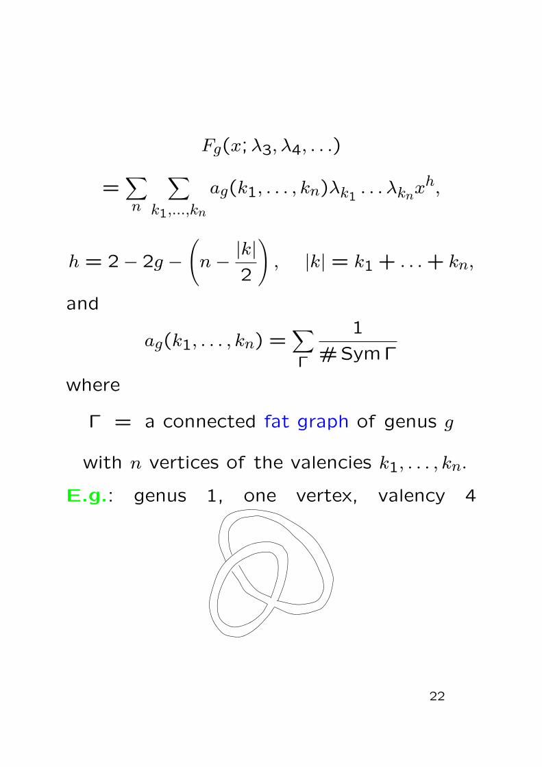
Fg(x;λ3, λ4, . . .)
=∑n
∑k1,...,kn
ag(k1, . . . , kn)λk1 . . . λknxh,
h = 2− 2g −(n−
|k|2
), |k| = k1 + . . .+ kn,
and
ag(k1, . . . , kn) =∑Γ
1
#SymΓ
where
Γ = a connected fat graph of genus g
with n vertices of the valencies k1, . . . , kn.
E.g.: genus 1, one vertex, valency 4
22
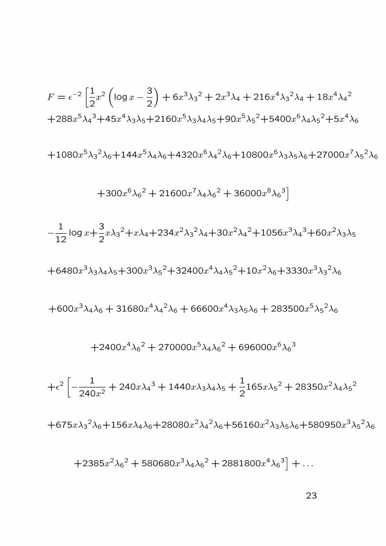
F = ε−2[1
2x2(logx−
3
2
)+ 6x3λ3
2 + 2x3λ4 + 216x4λ32λ4 + 18x4λ4
2
+288x5λ43+45x4λ3λ5+2160x5λ3λ4λ5+90x5λ5
2+5400x6λ4λ52+5x4λ6
+1080x5λ32λ6+144x5λ4λ6+4320x6λ4
2λ6+10800x6λ3λ5λ6+27000x7λ52λ6
+300x6λ62 + 21600x7λ4λ6
2 + 36000x8λ63]
−1
12logx+
3
2xλ3
2+xλ4+234x2λ32λ4+30x2λ4
2+1056x3λ43+60x2λ3λ5
+6480x3λ3λ4λ5+300x3λ52+32400x4λ4λ5
2+10x2λ6+3330x3λ32λ6
+600x3λ4λ6 + 31680x4λ42λ6 + 66600x4λ3λ5λ6 + 283500x5λ5
2λ6
+2400x4λ62 + 270000x5λ4λ6
2 + 696000x6λ63
+ε2[−
1
240x2+ 240xλ4
3 + 1440xλ3λ4λ5 +1
2165xλ5
2 + 28350x2λ4λ52
+675xλ32λ6+156xλ4λ6+28080x2λ4
2λ6+56160x2λ3λ5λ6+580950x3λ52λ6
+2385x2λ62 + 580680x3λ4λ6
2 + 2881800x4λ63]+ . . .
23
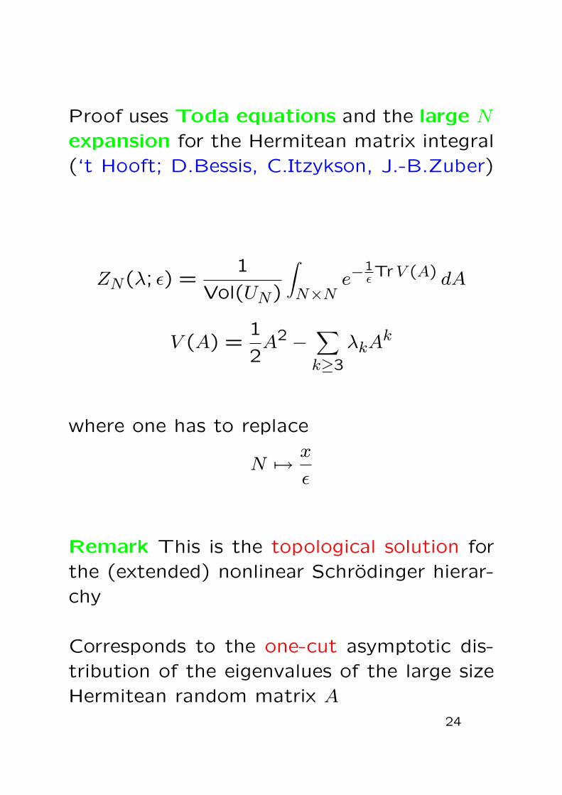
Proof uses Toda equations and the large N
expansion for the Hermitean matrix integral(‘t Hooft; D.Bessis, C.Itzykson, J.-B.Zuber)
ZN(λ; ε) =1
Vol(UN)
∫N×N
e−1εTr V (A) dA
V (A) =1
2A2 −
∑k≥3
λkAk
where one has to replace
N 7→x
ε
Remark This is the topological solution forthe (extended) nonlinear Schrodinger hierar-chy
Corresponds to the one-cut asymptotic dis-tribution of the eigenvalues of the large sizeHermitean random matrix A
24

Multicut case: gaps in the asymptotic dis-
tribution of eigenvalues of random matrices
⇒ singular behaviour of the correlation func-
tions (terms ∼ ei a tε arise)
(from Jurkiewicz, Phys. Lett. B, 1991)
Smoothed correlation functions: average
out the singular terms
Question: Which integrable PDEs describe
the large N expansion of smoothed correla-
tion functions?25
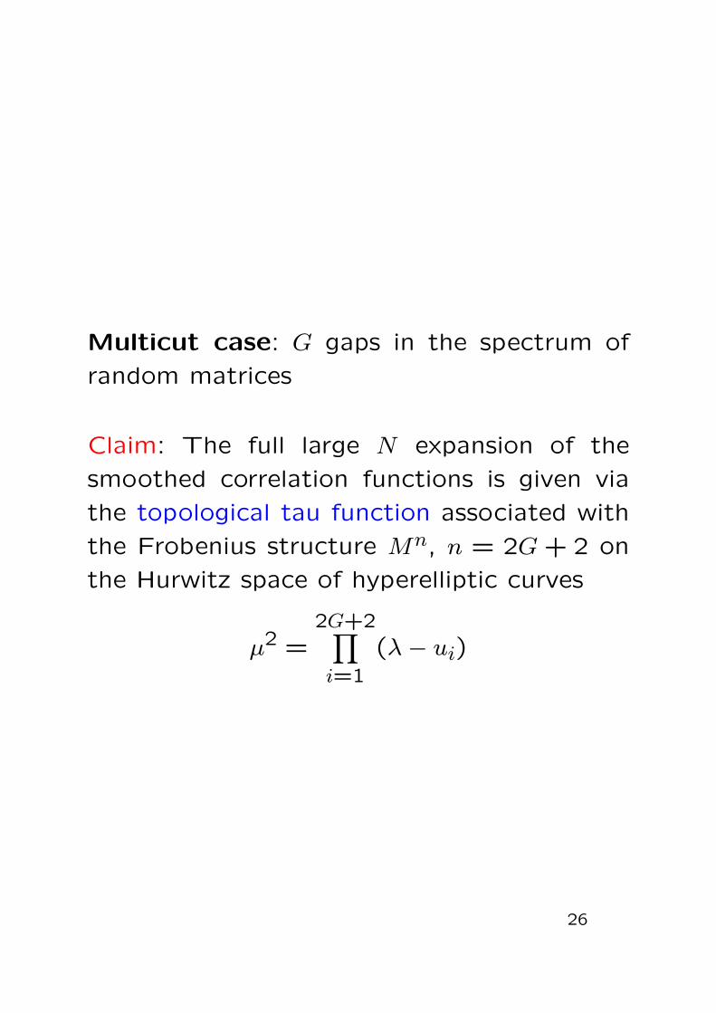
Multicut case: G gaps in the spectrum of
random matrices
Claim: The full large N expansion of the
smoothed correlation functions is given via
the topological tau function associated with
the Frobenius structure Mn, n = 2G+ 2 on
the Hurwitz space of hyperelliptic curves
µ2 =2G+2∏i=1
(λ− ui)
26
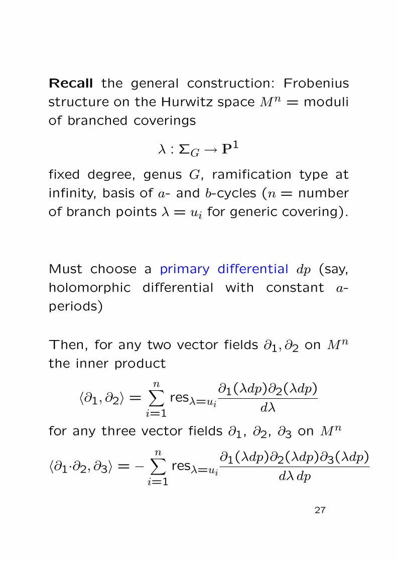
Recall the general construction: Frobenius
structure on the Hurwitz space Mn = moduli
of branched coverings
λ : ΣG → P1
fixed degree, genus G, ramification type at
infinity, basis of a- and b-cycles (n = number
of branch points λ = ui for generic covering).
Must choose a primary differential dp (say,
holomorphic differential with constant a-
periods)
Then, for any two vector fields ∂1, ∂2 on Mn
the inner product
〈∂1, ∂2〉 =n∑i=1
resλ=ui
∂1(λdp)∂2(λdp)
dλ
for any three vector fields ∂1, ∂2, ∂3 on Mn
〈∂1·∂2, ∂3〉 = −n∑i=1
resλ=ui
∂1(λdp)∂2(λdp)∂3(λdp)
dλ dp
27

Example G = 1 (two-cut case). Here n = 4.
Flat coordinates on the Hurwitz space of el-
liptic double coverings with 4 branch points
are u, v, w, τ . Can describe by the superpo-
tential (= symbol of Lax operator)
λ(p) = v+ u
(log
θ1(p− w|τ)θ1(p+ w|τ)
)′The Frobenius structure given by
F =i
4πτ v2 − 2u v w+ u2 log
[1
π u
θ1(2w|τ)θ′1(0|τ)
]
Recall
log
[θ1(x|τ)π θ′1(0|τ)
]= log sinπ x+ 4
∞∑m=1
q2m
1− q2msin2 πmx
m
q = ei π τ
28
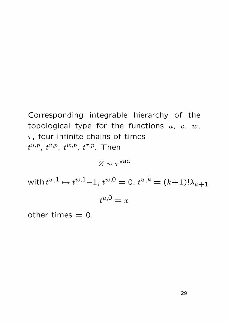
Corresponding integrable hierarchy of the
topological type for the functions u, v, w,
τ , four infinite chains of times
tu,p, tv,p, tw,p, tτ,p. Then
Z ∼ τvac
with tw,1 7→ tw,1−1, tw,0 = 0, tw,k = (k+1)!λk+1
tu,0 = x
other times = 0.
29
The solution is given via zero section of the
Lagrangian manifold{p = dΦx, λ
}∩ {p = 0}
Φx, λ = xw − u v+ u2P1(2w|τ)
+3λ3u[v2 − 2u v P1(2w|τ) + u2
(P 2
1 (2w|τ)− P2(2w|τ) + 4π i(log η(τ))′)]
+2λ4u[2v3 − 6u v2P1(2w|τ) + 6u2v
(P 2
1 (2w|τ)− P2(2w|τ) + 4π i(log η(τ))′)
−u3[P3(2w|τ) + 2P1(2w|τ)
(P1(2w|τ)2 − 3P2(2w|τ) + 12π i (log η(τ))′
)]]+ . . .
where
Pk(x|τ) := ∂kx log θ1(x|τ), k = 1,2,3
Canonical coordinates (branch points)
ui = v − 2u [log θi(w|τ)]′, i = 1, . . . ,4.
ε2-correction
F1 = −1
6logu− log η(2τ) +
1
24
4∑i=1
logu′i
30

General structure of solutions for
• t < tc: regular ε-expansions, quasitriviality
• t ∼ tc: special solutions to Painleve-type
equations, universality
• t > tc: regular ε-expansions, quasitriviality
for new system of PDEs, phase transitions
31