Strategic or Non-Strategic: The Role of Financial Benefit in Bankruptcy

By

Shuoxun Zhang , Tarun Sabarwal, and Li Gan1

This version: July 16, 2014

Abstract

A partial test for strategic behavior in bankruptcy filing may be formulated by testing whether consumers manipulate their debt and filing decision jointly, or not: that is, testing for endogeneity of financial benefit and the bankruptcy filing decision. Using joint maximum likelihood estimation of an extended discrete choice model, test results are consistent with non-strategic filing: financial benefit is exogenous to the filing decision. This result is confirmed in two different datasets (PSID and SCF). This result is consistent with an ex ante low net gain from a bankruptcy filing; a type of “rational inattention” to rare events such as bankruptcy.

Keywords: Consumer bankruptcy, personal bankruptcy, adverse events, strategic filing JEL Classification: D12, D14

1Zhang: Research Institute of Economics and Management, Southwestern University of Finance and

Economics, Chengdu, China, shuoxun@swufe.edu.cn

Sabarwal: Department of Economics, University of Kansas, sabarwal@ku.edu

Gan: Department of Economics, Texas A&M University, and NBER, gan@econmail.tamu.edu.

1

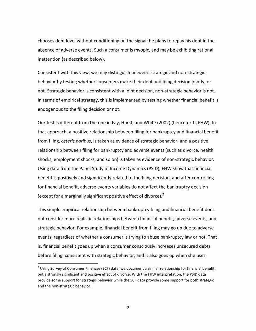
1. Introduction

Personal bankruptcy rates have increased at an annual rate of 3.9 percent since 1990,

from about 718 thousand (non-business) bankruptcies in 1990 to about 1.5 million in

2010. Partly as a response to this increase, the Congress passed the Bankruptcy Abuse

Prevention and Consumer Protection Act of 2005, the largest overhaul of bankruptcy

laws since 1980. Although recent data is too sparse to determine the longer-term

effectiveness of the law, we know that there was a spike in bankruptcy filings in 2005

(just before the law took effect on October 17, 2005) and a corresponding decline in

2006. Since then, bankruptcies have continued to rise, reaching a level of about 1.5

million in 2010, the same level as in 2004. (The bankruptcy rate has also begun to creep

up to the earlier levels.) One of the major purposes of the new bankruptcy law was to

cut down on abusive or fraudulent uses of the bankruptcy system, or in our words,

strategic use of the law. Therefore, it is important to understand the motivations of

consumers who file for bankruptcy, what constitutes “strategic” use of bankruptcy law,

and how widespread is its incidence.

In the literature, there is no clear definition of what constitutes a strategic bankruptcy

filing. We shall consider strategic behavior to be a conscious decision to benefit from

bankruptcy law. To make this tractable, consider a simple two-period model of decision-

making. In the first period, consumers receive a noisy signal of experiencing a financial

shock in the second period. Based on this signal, consumers may update their

probability of an adverse shock and choose their debt level. In the second period, the

shock is realized and consumers decide whether to file for bankruptcy or not. A strategic

consumer is one who in the first period, chooses her debt level after conditioning on the

signal; that is, a strategic consumer takes on debt after accounting for the chance of

filing for bankruptcy. In other words, a strategic consumer is one who is fully rational,

and takes decisions to maximize her benefit. A non-strategic consumer is one who

2

chooses debt level without conditioning on the signal; he plans to repay his debt in the

absence of adverse events. Such a consumer is myopic, and may be exhibiting rational

inattention (as described below).

Consistent with this view, we may distinguish between strategic and non-strategic

behavior by testing whether consumers make their debt and filing decision jointly, or

not. Strategic behavior is consistent with a joint decision, non-strategic behavior is not.

In terms of empirical strategy, this is implemented by testing whether financial benefit is

endogenous to the filing decision or not.

Our test is different from the one in Fay, Hurst, and White (2002) (henceforth, FHW). In

that approach, a positive relationship between filing for bankruptcy and financial benefit

from filing, ceteris paribus, is taken as evidence of strategic behavior; and a positive

relationship between filing for bankruptcy and adverse events (such as divorce, health

shocks, employment shocks, and so on) is taken as evidence of non-strategic behavior.

Using data from the Panel Study of Income Dynamics (PSID), FHW show that financial

benefit is positively and significantly related to the filing decision, and after controlling

for financial benefit, adverse events variables do not affect the bankruptcy decision

(except for a marginally significant positive effect of divorce).2

This simple empirical relationship between bankruptcy filing and financial benefit does

not consider more realistic relationships between financial benefit, adverse events, and

strategic behavior. For example, financial benefit from filing may go up due to adverse

events, regardless of whether a consumer is trying to abuse bankruptcy law or not. That

is, financial benefit goes up when a consumer consciously increases unsecured debts

before filing, consistent with strategic behavior; and it also goes up when she uses

2 Using Survey of Consumer Finances (SCF) data, we document a similar relationship for financial benefit,

but a strongly significant and positive effect of divorce. With the FHW interpretation, the PSID data

provide some support for strategic behavior while the SCF data provide some support for both strategic

and the non-strategic behavior.

3

unsecured debt (e.g. a credit card) to pay for expenses due to adverse events, consistent

with non-strategic behavior. Moreover, a non-strategic consumer may appear strategic

to the analyst, if he rolls over debt as long as there is hope of repaying it. This leads to

greater measured financial benefit before filing, despite no intent to abuse bankruptcy

law. Indeed, equilibrium models of default typically include such features.3

In other words, financial benefit is affected by both strategic and non-strategic behavior,

and a positive coefficient on financial benefit alone is insufficient to distinguish between

the two behaviors.4

Our test partially disentangles the role of financial benefit, adverse events, and strategic

behavior: it allows for a positive relationship between bankruptcy filing and financial

benefit for both strategic and non-strategic consumers and still may distinguish

between the two. This test cannot distinguish between strategic consumers and non-

strategic consumers who may appear strategic due to a non-strategic run-up of debt

before filing.

Consequently, if the test result shows that financial benefit is endogenous to the filing

decision, that result can be consistent with both strategic and non-strategic behavior. If

the test result shows that financial benefit is exogenous to the filing decision, the result

supports non-strategic filing behavior (and shows that the incidence of both strategic

3The literature on consumer bankruptcy is very large. A partial list includes the following. Stanley and

Girth (1971) and Eaton and Gersovitz (1981) present early work in this area. Additional work includes

Sullivan, Warren, and Westbrook (1989, 1994, and 2000), White (1987, 1998), Ausubel (1991, 1997),

Domowitz and Sartain (1999), Gross and Souleles (2002), Fay, Hurst, and White (2002), Fan and White

(2003), Han and Li (2004), and Livshits, Macgee, and Tertilt (2007, 2010). Athreya (2005) provides a survey

of equilibrium models of default. Additional theoretical contributions include Zame (1993), Modica,

Rustichini, and Tallon (1999), Araujo and Pascoa (2002), Sabarwal (2003), Dubey, Geanakoplos, and Shubik

(2005), Geanakoplos and Zame (2007), and Hoelle (2009), among others. 4 This point may be made more generally: we show that in the standard random utility model underlying

the binary choice of filing and not filing, the coefficient on unsecured debt (and hence, on financial benefit

from filing) is positive, regardless of how debt is accumulated.

4

filings and non-strategic filings that may appear strategic is statistically insignificant in

the data).

We propose a model in which financial benefit and the filing decision are jointly

determined, estimate it using joint maximum likelihood, and test for endogeneity of

financial benefit and the filing decision. The discussion provides a set of natural

instrumental variables, the adverse events.

Using two different datasets (PSID and SCF),5 the test results are consistent with non-

strategic behavior, in contrast to FHW. With both datasets, financial benefit is

exogenous to the filing decision. Moreover, with both datasets, the coefficient on

financial benefit is strongly significantly positive.

Our finding is consistent with “rational inattention” to rare events such as bankruptcy;

that is, ex ante, the benefit from a bankruptcy filing is very low relative to costs, leaving

little incentive for consumers to actively “plan” to file for bankruptcy. For example, as

reported in FHW, for families that can gain from a bankruptcy filing, the mean benefit

from filing is $7,813, and the probability of filing is 0.003017, for an ex-ante filing benefit

of about $25. This is less than the cost of a planning session with a bankruptcy lawyer,

or the resources expended to purchase and plan with a book on how to file for

bankruptcy. Note that planning for a strategic bankruptcy would have to be done early

enough, because legal restrictions disallow wealth re-allocations designed to gain from

bankruptcy, especially if these are within about six months prior to a bankruptcy filing.

The paper proceeds as follows. Section 2 describes the basic theory and a theoretical

result on positive correlation between financial benefit and filing probability. Section 3

presents the econometric specifications, and results, and section 4 concludes.

5Although both PSID and SCF are among the best publicly available datasets of their kind, they have well-

known limitations for bankruptcy research. Using two datasets provides some robustness to these results,

but better bankruptcy data would help to arrive at stronger conclusions.

5

2. Basic theory and Positive Correlation between Financial Benefit and

Filing Probability

Bankruptcy filers typically have a choice between filing for Chapter 7 or Chapter 13

bankruptcy.6 A Chapter 7 bankruptcy process liquidates a filer’s estate, and net of

exemptions, makes payments to creditors based on law. This is sometimes termed a

straight bankruptcy. In a Chapter 13 filing, a filer typically keeps his assets, proposes a

plan of repayment, and on plan completion, gets discharge from remaining debts.

Historically, about 70 percent of bankruptcies are Chapter 7, and most of the remainder

are Chapter 13. Moreover, a filing under Chapter 13 may be moved to Chapter 7, if the

Chapter 13 repayment plan is not completed successfully. In practice, this can happen in

a significant proportion of Chapter 13 filings.7 Therefore, most research models Chapter

7 bankruptcy filing. We follow the same approach.8

Consider a simple two-period model of decision-making. Prior to the first period,

consumers receive a noisy signal of experiencing a financial shock. The shock may be

viewed as an adverse event: job loss, health problem, divorce, and so on. Based on this

signal, consumers may update their probability of an adverse shock. In the first period,

they choose their debt level. Then the shock is realized and in the second period,

consumers decide whether to file for bankruptcy or not.

6 Before BAPCPA, consumers had more freedom in choosing the chapter in which to file. After BAPCPA,

choice is restricted by a “means” test(§ 707(b)(2)). Given the high rate of failures of Chapter 13 plans, it is

as yet unclear how many consumers required to file under Chapter 13 eventually end up with a discharge

under Chapter 7. The analysis here and the dataset used are for filings before BAPCPA.

7 Sullivan, Warren, and Westbrook (2000, p. 14) estimate this to be about two-thirds of Chapter 13 filings.

8 A Chapter 13 filing may be viewed as a reduced form Chapter 7 filing, where debt recovery is the total

amount repaid over the course of the proposed plan. We do not force such an interpretation.

6

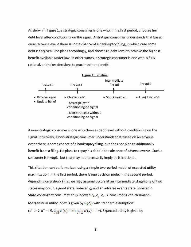
As shown in figure 1, a strategic consumer is one who in the first period, chooses her

debt level after conditioning on the signal. A strategic consumer understands that based

on an adverse event there is some chance of a bankruptcy filing, in which case some

debt is forgiven. She plans accordingly, and chooses a debt level to achieve the highest

benefit available under law. In other words, a strategic consumer is one who is fully

rational, and takes decisions to maximize her benefit.

A non-strategic consumer is one who chooses debt level without conditioning on the

signal. Intuitively, a non-strategic consumer understands that based on an adverse

event there is some chance of a bankruptcy filing, but does not plan to additionally

benefit from a filing. He plans to repay his debt in the absence of adverse events. Such a

consumer is myopic, but that may not necessarily imply he is irrational.

This situation can be formalized using a simple two-period model of expected utility

maximization. In the first period, there is one decision node. In the second period,

depending on a shock (that we may assume occurs at an intermediate stage) one of two

states may occur: a good state, indexed g, and an adverse events state, indexed a.

State-contingent consumption is indexed . A consumer’s von-Neumann-

Morgenstern utility index is given by , with standard assumptions

( ). Expected utility is given by

Intermediate Period Period 2

Period 1

Choose debt

- Strategic: with conditioning on signal

- Non-strategic: without conditioning on signal

Filing Decision

Figure 1: Timeline

Shock realized

Period 0

Receive signal

Update belief

7

, where the distribution captures uncertainty in

the second stage. Consumer’s state-contingent wealth is given by . For

convenience, we assume .

Consumption in first period is financed by debt , available at a (risk-adjusted)

interest rate .9 For non-trivial solution, we assume debt limit for a consumer is

given by , so that is constrained to satisfy . Exemptions in bankruptcy are

given by . A natural assumption in this setting is .

A strategic consumer is fully rational, maximizing

subject to (1) (2) , and (3)

. Here, is the (updated) belief of the

probability of an adverse event, based on the signal received. The minimum operation is

a proxy for loss of non-exempt assets in a bankruptcy filing, and the maximum operation

corresponds to the bankruptcy decision: file when non-exempt assets are greater than

net wealth remaining after debt repayment. The effective decision variable is . Notice

that our assumptions imply that in the adverse event state, the consumer files for

bankruptcy and consumes .

A non-strategic consumer does not condition debt decision on the adverse events signal

captured by the (updated) distribution . Such a consumer may be viewed as

taking decision sequentially. In period 1, the consumer maximizes ,

subject to (1) and (2) . Effectively, a non-strategic

consumer is not planning for a bankruptcy filing and plans to repay his debt in period 2.

If, however, an adverse event occurs in period 2, the consumer re-optimizes to set

9 This is a simple model of individual decision-making, not general equilibrium. We take the risk-adjusted

interest rate (price of debt) as given.

8

. Our assumptions imply that in the adverse

events state, consumer files for bankruptcy and consumes .

By construction, this formulation shows immediately that for a strategic consumer, debt

and filing decision are determined jointly, whereas for a non-strategic consumer, this is

not the case.10 Moreover, a strategic consumer may file for bankruptcy in a good state

(in which exemption is low relative to wealth), if debt elimination from bankruptcy can

offset the loss of non-exempt assets. A non-strategic consumer does not engage in such

behavior.

One way to motivate non-strategic behavior is in terms of rational inattention to rare

events. In other words, ex-ante, a non-strategic consumer behaves as if his subjective

probability of an adverse event is zero. This might not necessarily be irrational, if we

expand the model to include some ex-ante cost of determining the probability of an

adverse event and planning for a bankruptcy filing, and the ex-ante benefit from a

bankruptcy filing, and then consider a behavioral choice whether a consumer would

want to behave strategically or non-strategically. Such an extension is beyond the scope

of this paper, but as reported in FHW, for families that can gain from a bankruptcy filing,

the mean benefit from filing is $7,813, and the probability of filing is 0.003017, for an

ex-ante filing benefit of about $25. If a consumer were to plan to gain from a bankruptcy

filing, he would include the ex-ante cost of a planning session with a bankruptcy lawyer,

or the resources expended to purchase and plan with a book on how to file for

bankruptcy; this is typically greater than $25. This would have to be done early enough,

because legal restrictions disallow wealth re-allocations designed to gain from

bankruptcy, especially if these are within about six months prior to a bankruptcy filing.

10

Using standard assumptions, it is easy to show that both problems have an interior solution, and

optimal debt for a strategic consumer is (weakly) greater than that for a non-strategic consumer.

9

An immediate consequence of this model is that for a strategic consumer, financial

benefit is endogenous to the filing decision, and for a non-strategic consumer, it is

exogenous. This leads us to the empirical test used here.

As mentioned above, this empirical test only partly disentangles the endogeneity,

because even for a non-strategic consumer, there might be some debt accumulation

after the shock is realized, if the consumer is trying to roll over debt with the hope of

repaying it. But a finding of exogeneity favors non-strategic behavior.

In empirical work, filing for bankruptcy is typically modeled as a binary choice model.

FHW indicate that a positive and significant relationship between household financial

benefit and probability of filing for bankruptcy signals strategic behavior by a consumer.

Similarly, Adams, Einav, and Levin (2009) suggest that an increase in probability of

default with loan size is consistent with either moral hazard behavior or adverse

selection behavior. In the same spirit, we show that financial benefit may affect the

probability of filing, regardless of how debt is accumulated.

According to McFadden’s Random Utility Maximization model, the probability that a

person files for bankruptcy is increasing in the utility difference between filing and not

filing. To investigate this difference, let d be unsecured debt and w be assets minus

secured debt. For simplicity, the exemptions are normalized to be zero. Financial benefit

from filing, given d, is 0,max, wddfileB , and financial benefit from not filing,

given d, is 0,max, dwdNotB . Notice that dNotBdfileB ,, if and only if d

≥ w.

Let u denote utility from monetary outcomes. Assume that u is strictly increasing and

continuously differentiable. We may write utility from filing, given d as:

dfileBudfileU ,, ; utility from not filing, given d as dNotBudNotU ,, ; and

the difference in these utilities is dNotUdfileUdU ,, . Therefore,

10

dNotBdNotBudfileBdfileBudU ,',',','' .

Consider the following cases. Case 1: d > w. In this case, 1,' dfileB

and 0,' dNotB . Therefore, 0,'' dNotBudU . Case 2: d < w. In this case,

0,' dfileB and 1,' dNotB , whence, 0,'' dNotBudU . Case 3: d = w.

In this case, 00',','lim

uwfileBudfileBuwd

, and

similarly, 00',','lim

uwNotBudNotBuwd

. In all cases, we have 0' dU .

In terms of empirical prediction, this implies that the coefficient on unsecured debt (and

consequently, on financial benefit from filing) is positive, regardless of how debt is

accumulated.11 Therefore, given unsecured debt d, a positive relationship between

financial benefit from filing and filing for bankruptcy is expected.

3. Econometric Models and Results

In this section, we first provide some information on the data and construction of

variables. Next, we replicate the FHW’s specification using two different datasets. Then

we present test results for endogeneity of financial benefit (using joint maximum

likelihood estimation) with two different datasets. Finally, we use comparative statistics

to predict the bankruptcy filing rates with hypothetical changes in key variables.

3.1 Data description and variables

We use two different datasets to check robustness of our results. One is the combined

cross-section and time series sample of PSID households over the period 1984-1995; the

11

Notice that all we used here was that u is strictly increasing and continuously differentiable. No

additional restriction is imposed on utility.

11

same dataset is used in FHW. The other is the cross sectional dataset of SCF from

1998.12

In 1996, the PSID asked respondents whether they had ever filed for bankruptcy and if

so, in which year. This information, combined with other household characteristics

forms the basis of our first dataset. The PSID data are generally of high quality, but they

have some limitations for a study of this kind. In particular, wealth is only measured at

5-year intervals, and it contains less detail on some aspects of use in this study.

Moreover, as documented in FHW, there are only 254 bankruptcy filings over the period

1984-1995, and bankruptcy filings in the PSID are only about one-half of the national

filing rate.

SCF, in contrast, has 55 bankruptcy filings in 1997, or about 1.28 percent of households,

comparable to the 1997 national bankruptcy filing rate of 1.16 percent. The SCF is cross-

sectional only, so we lose the time-series aspect in this case; but there is some

information for the year prior to the survey, and on future expectations.

SCF also provides better wealth data, which reports 1997 wealth information and 1997

bankruptcy filings. (The SCF survey was conducted in 1998, between June and

December.) 13

We do not distinguish Chapter 7 and Chapter 13 filings in this paper (although

consumers are able to make choices), because the financial benefit from filing under

Chapter 13 is closely related to that from filing under Chapter 7. It usually takes

between four and six months for a Chapter 7 filing procedure, but between 36 and 60

months for a typical Chapter 13 case. The 1998 SCF does not provide information on

12

SCF asks the respondents about their bankruptcy history, but the region/state in which they stay is not

revealed to the public after 1998. In order to match the two datasets, we choose the data of the most

recent year. 13

See Kennickell et. al (1998).

12

chapter choice. Financial benefit from filing is the key variable in this paper. As in FHW,

it is calculated as follows:

,

where is the financial benefit from filing for household i in period t, is the

unsecured debt discharged in bankruptcy for household i in period t, is the value of

wealth for household i in period t, and is value of exemptions under law for

household i in period t, in the household’s state of residence. In this formula,

calculates the nonexempt assets that a filer loses in bankruptcy. It is

a measure of financial cost of filing for bankruptcy. The variable is the part that will

be discharged in bankruptcy, thus is a measure of benefit of filing. As not filing

dominates filing when is negative, the financial benefit from

filing is truncated at 0 to yield the above formula.

Notice that this calculation does not include the full economic cost of a bankruptcy

filing. For example, a more complete measure of the economic cost of filing would

include future and dynamic costs of a bankruptcy filing as well, such as loss of future

stream of profits from liquidated assets, or effects on future credit-worthiness, which

determines future access to debt markets and the price of debt. A more complete

accounting of the cost of bankruptcy would include such costs and also out-of-pocket

filing costs. Reliable data on these measures is unavailable, and including a reduced

form constant would not change the qualitative results. This is a limitation of our

approach, as also that of FHW.

To calculate financial benefit in the PSID, we use the same dataset and calculation as

FHW. In the PSID, housing equity is reported every year, but non-housing wealth is

reported only in the 5-yearly wealth supplements from 1984, 1989, and 1994. These

data are used to construct unsecured debt, , that will be discharged in bankruptcy.

13

Wealth includes current year housing equity (reported every year) and the value of the

most recent prior report on non-housing wealth.14 , is the wealth net of secured

debts (like mortgages and car loans). Exemption, , is the exemption in the state of

residence of household i in period t.

For the SCF, variables are constructed similarly. The variable measures unsecured

debt that will be discharged in bankruptcy. Unsecured debts include both credit card

debt and installment loans.15 Wealth , is total assets net of the secured debt. Total

assets include all financial assets and non-financial assets.16 For exemption, , we

make the following adjustments.

The SCF provides only region codes; state codes are not released in public data. To get a

relative weight for each state in a region, we use Regional Economic Information System

(REIS) from the Bureau of Economic Analysis. These state weights are based on the

population of a state relative to the region in which it is included. These weights are

used to compute the composite exemption level of a region. Moreover, using Elias,

Renauer, and Leonard (1999), we determine each state’s exemption levels for 1998 for

homestead equity in owner-occupied homes, equity in vehicles, personal property, and

14

Data on unsecured debt and non-housing wealth is subject to measurement error and therefore

financial benefit is subject to measurement error, but as reported in FHW, this does not significantly

affect the results.

15 Credit card debt includes not only the traditional Visa/Mastercard/Discover/Optima cards, but also

revolving debts at stores, including store cards, gasoline cards, airline cards and diner club cards.

Installment loans refer to those for purposes other than purchasing houses or real estates.

16 Financial assets are the sum of all types of transactions accounts(checking accounts, saving accounts,

money market accounts and call accounts), certificates of deposits, total directly-held mutual funds,

bonds, stocks, total quasi-liquid(sum of IRAs, thrift accounts, and future pensions), saving bonds, cash

value of whole life insurance, other managed assets (trusts, annuities and managed investment accounts

in which household has equity interest), other financial assets: includes loans from the household to

someone else, future proceeds, royalties, futures, non-public stock, deferred compensation,

oil/gas/mineral investments, and cash not elsewhere classified.

14

wildcard exemptions. We adjust for state level variables to the extent we can. For

example, if a state doubles exemptions for married households, we do the same. For the

fifteen states allowing residents to choose between state or federal exemptions, we

take the larger of the exemptions. For households in states with an unlimited

homestead exemption, we take the homestead exemption to be the average of home

values in the entire sample. The exemption variable, , is the sum of these

exemptions. 17To make the two datasets consistent with each other, we include a vector

of demographic variables which may be related to households’ filing decisions, such as

age of household head, years of education of the head, family size, whether head owns

their home and whether head owns business. For SCF data, we include only region

dummies rather than macro information to capture local fixed effects, due to lack of

information regarding state of residency.

For adverse events variables, we include whether the head was ever unemployed during

the prior twelve months (labeled “unemployed”), total weeks of unemployment during

the prior twelve months (labeled “period of unemployment”),18 its squared term,

whether the head is recently divorced (labeled “divorce”),19 and whether the head’s

(self-reported) health condition is poor (labeled “health”).20

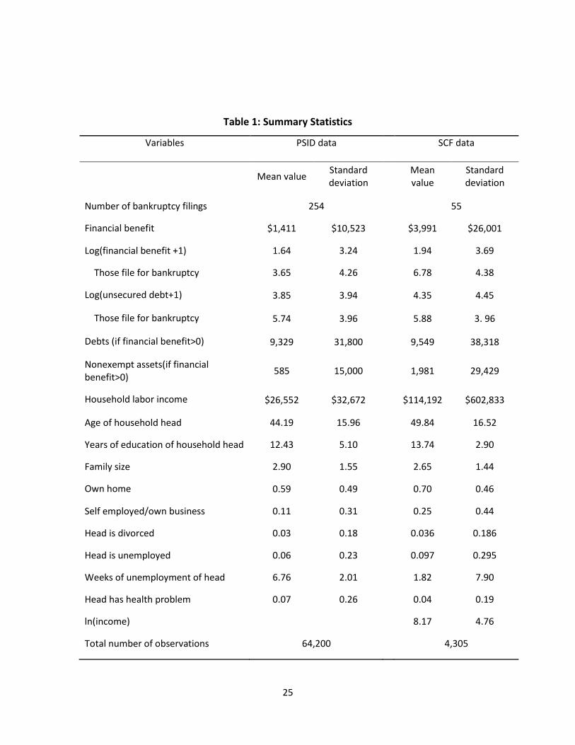
In table 1, we present financial benefit and unsecured debt between filers and non-filers

for both PSID and SCF. Similar patterns emerge. In PSID, the mean log(financial benefit)

17

The exemption levels calculated using PSID and using SCF have different advantages and flaws, and thus

subject to measurement errors, but it does not significantly affect the results.

18 We uniformly recode the variable to be 52 if the spell of unemployment is more than one year.

19 The reported results in Table 4 and 6 are using the dummy variable for divorce during years of 1996-

1998, but we have tried dummy variables for divorce of each year, which do not change the significance

of the result/coefficient.

20 We also tried the dummy for either the head or the partner was in poor health status. The results

remain robust.

15

for filers is more than twice as much than those non-filers. In SCF, filers have more than

three times as much mean log(financial benefit) than non-filers. In both SCF and PSID,

the mean log(unsecured debt) for filers is greater than that of non-filers.

As in FHW, our debt calculation is for the period of filing, and the adverse events

variables are for the prior period. This is consistent with our model (with adverse events

realized before the bankruptcy decision).

There is the issue that in the data, it is possible that debt (and therefore, financial

benefit) changes after an adverse event occurs and before a bankruptcy filing. We can

consider two cases.

First, an adverse event (which here is assumed to occur with an exogenous probability)

itself leads to an increase in debt. This is captured in the model in a reduced form by a

reduction in state-contingent wealth, and empirically in the financial benefit calculation.

Second, a consumer might take some actions that change debt just before filing. For

example, a strategic consumer could try and consciously increase unsecured debts just

before filing in order to increase benefit from filing. As mentioned above, there are legal

restrictions for such moves and creditors are likely to have these enforced strictly. On

the other hand, debt may go up when a non-strategic consumer rolls over debt in the

hope of repaying it. As mentioned earlier, our test cannot distinguish between strategic

consumers and non-strategic consumers who may appear strategic due to a non-

strategic run-up of debt before filing.

Consequently, if the test result shows that financial benefit is endogenous to the filing

decision, that result can be consistent with both strategic and non-strategic behavior. If

the test result shows that financial benefit is exogenous to the filing decision, the result

supports non-strategic filing behavior (and shows that the incidence of both strategic

16

filings and non-strategic filings that may appear strategic is statistically insignificant in

the data).

3.2 Simple Probit model

Let’s first consider a simple Probit regression, similar to FHW’s specification.

This specification explores strategic and non-strategic behavior by running the Probit

regression of whether households file for bankruptcy (file) as a function of their

potential financial benefit, , from filing, their personal and state characteristics , and

the adverse events they encountered in the previous year, .

As described above, one test of strategic behavior focuses on the significance of the

coefficients on financial benefit and on adverse events, as in FHW. If strategic behavior

hypothesis is true, the coefficients of financial benefit should be positive and significant

while the adverse event variables should not be significant. If non-strategic behavior

hypothesis is true, then adverse event variables should be positive and significant while

the coefficient of financial benefit should be insignificant.

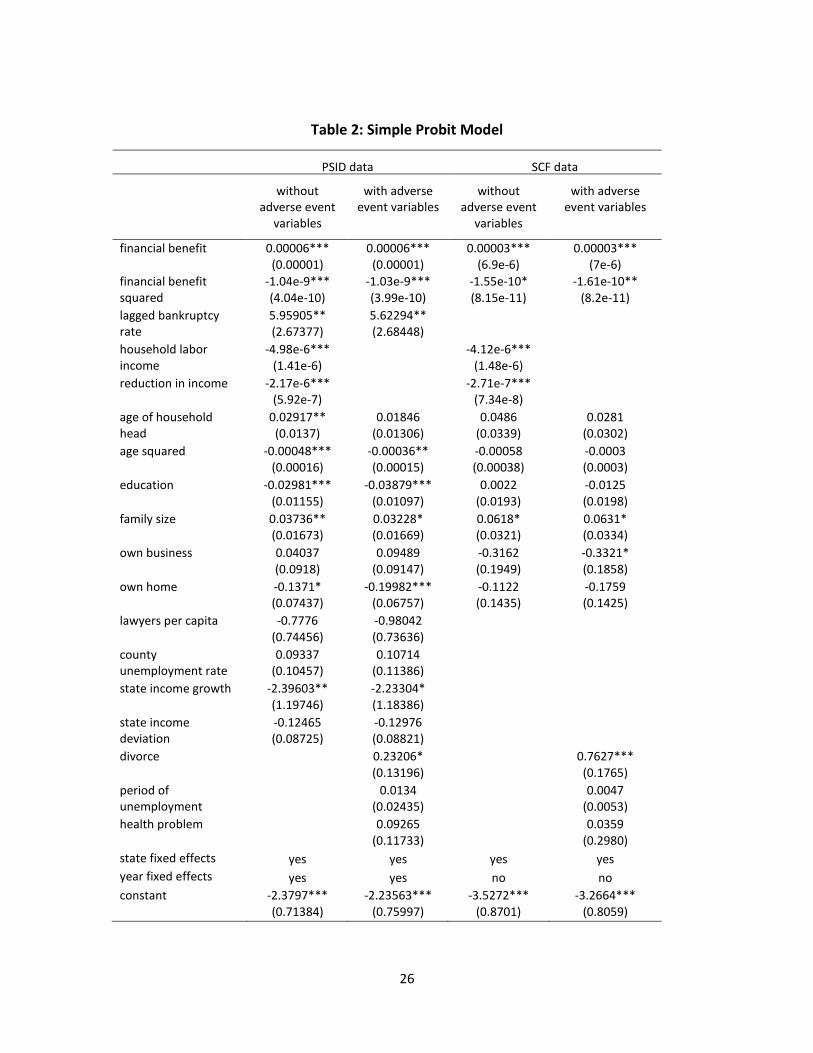
Table 2 illustrates this simple specification with PSID data and SCF data.21 (For ease of

comparison, we keep the other variables same as those in FHW.) As shown in table 2,22

using PSID data, the coefficients on the variables are comparable to those reported in

FHW. In particular, financial benefit affects the filing decision positively and highly

significantly, and its squared term is highly significant. And, among statistically

21

For all estimates, * indicates significance at 90 percent, ** at 95 percent, and *** at 99 percent. 22

The pseudo R-square for the four columns of Table 2 are 0.1378, 0.1320, 0.1377, and 0.1524,

respectively. The first two columns use the PSID family weights. Standard errors (in PSID) are corrected

using the Huber/White procedure, which allows error terms for the same household to be correlated over

time. We apply this procedure to table 3 and table 5, too.

17

significant adverse events, divorce is positive but only marginally significant. When using

SCF data, financial benefit continues to be positive and highly significant, but its squared

term is marginally significant. The coefficient on divorce remains positive, but is highly

significant.

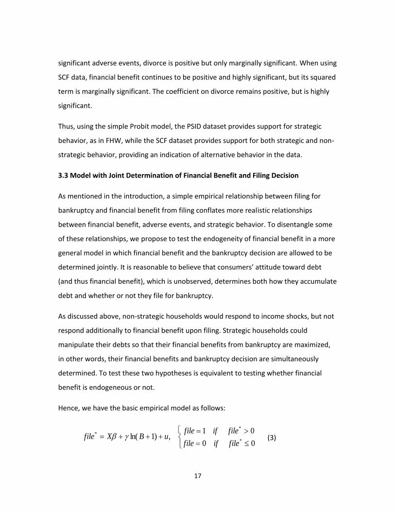
Thus, using the simple Probit model, the PSID dataset provides support for strategic

behavior, as in FHW, while the SCF dataset provides support for both strategic and non-

strategic behavior, providing an indication of alternative behavior in the data.

3.3 Model with Joint Determination of Financial Benefit and Filing Decision

As mentioned in the introduction, a simple empirical relationship between filing for

bankruptcy and financial benefit from filing conflates more realistic relationships

between financial benefit, adverse events, and strategic behavior. To disentangle some

of these relationships, we propose to test the endogeneity of financial benefit in a more

general model in which financial benefit and the bankruptcy decision are allowed to be

determined jointly. It is reasonable to believe that consumers’ attitude toward debt

(and thus financial benefit), which is unobserved, determines both how they accumulate

debt and whether or not they file for bankruptcy.

As discussed above, non-strategic households would respond to income shocks, but not

respond additionally to financial benefit upon filing. Strategic households could

manipulate their debts so that their financial benefits from bankruptcy are maximized,

in other words, their financial benefits and bankruptcy decision are simultaneously

determined. To test these two hypotheses is equivalent to testing whether financial

benefit is endogeneous or not.

Hence, we have the basic empirical model as follows:

00

01,)1ln(

*

*

*

fileiffile

fileiffileuBXfile (3)

18

00

0,)1ln(

*

**

*

BifB

BifBBvAXB (4)

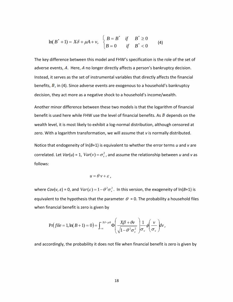
The key difference between this model and FHW’s specification is the role of the set of

adverse events, . Here, no longer directly affects a person’s bankruptcy decision.

Instead, it serves as the set of instrumental variables that directly affects the financial

benefits, , in (4). Since adverse events are exogenous to a household’s bankruptcy

decision, they act more as a negative shock to a household’s income/wealth.

Another minor difference between these two models is that the logarithm of financial

benefit is used here while FHW use the level of financial benefits. As depends on the

wealth level, it is most likely to exhibit a log-normal distribution, although censored at

zero. With a logarithm transformation, we will assume that v is normally distributed.

Notice that endogeneity of ln(B+1) is equivalent to whether the error terms u and v are

correlated. Let Var(u) = 1, 2)( vvVar , and assume the relationship between u and v as

follows:

vu ,

where Cov(v, ε) = 0, and 221)( vVar . In this version, the exogeneity of ln(B+1) is

equivalent to the hypothesis that the parameter = 0. The probability a household files

when financial benefit is zero is given by

AX

vvv

dvvvX

Bfile

1

10)1ln(,1Pr

22,

and accordingly, the probability it does not file when financial benefit is zero is given by

19

AX

vvv

dvvvX

Bfile

1

1-0)1ln(,0Pr

22.

Similarly,

vvv

AXBAXBBX

Bfile

)1ln(1

1

)1ln()1ln(

))1ln(,1Pr(

22

, and

vvv

AXBAXBfbX

Bfile

)1ln(1

1

)1ln()1ln(1

))1ln(,0Pr(

22

.

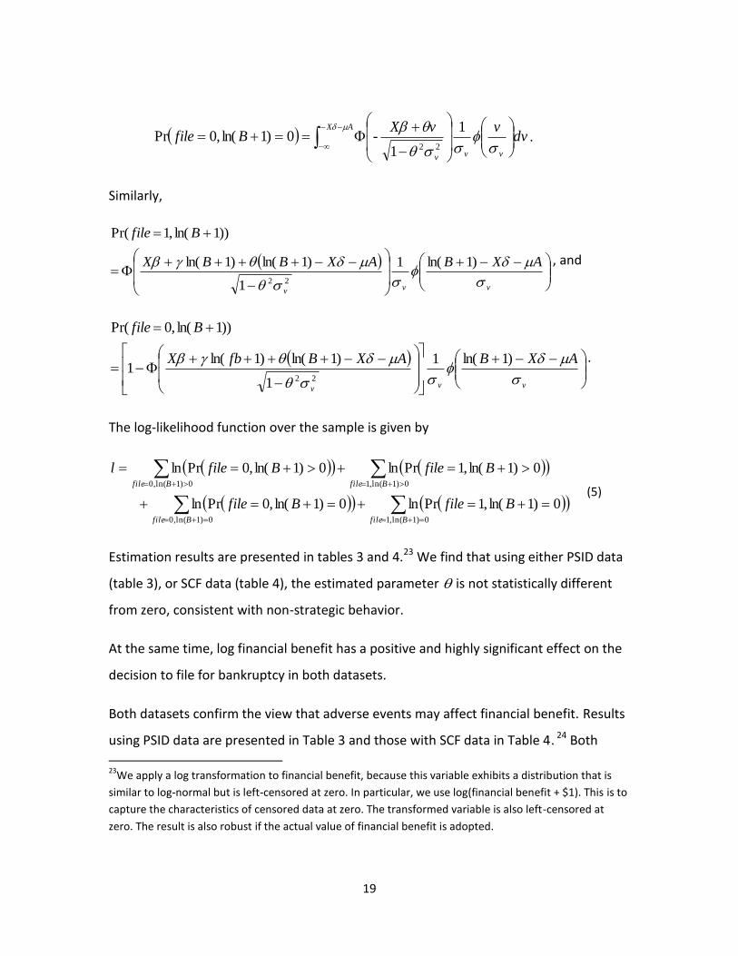
The log-likelihood function over the sample is given by

0)1ln(,10)1ln(,0

0)1ln(,10)1ln(,0

0)1ln(,1Prln0)1ln(,0Prln

0)1ln(,1Prln0)1ln(,0Prln

BfileBfile

BfileBfile

BfileBfile

BfileBfilel

(5)

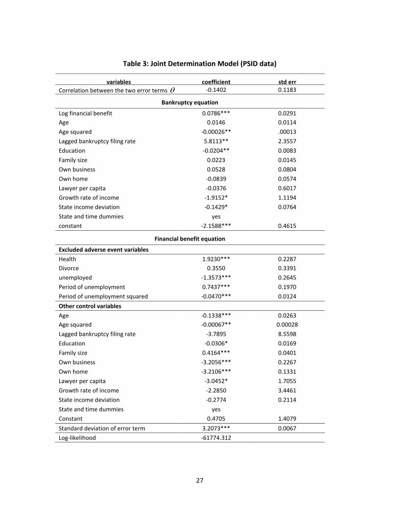
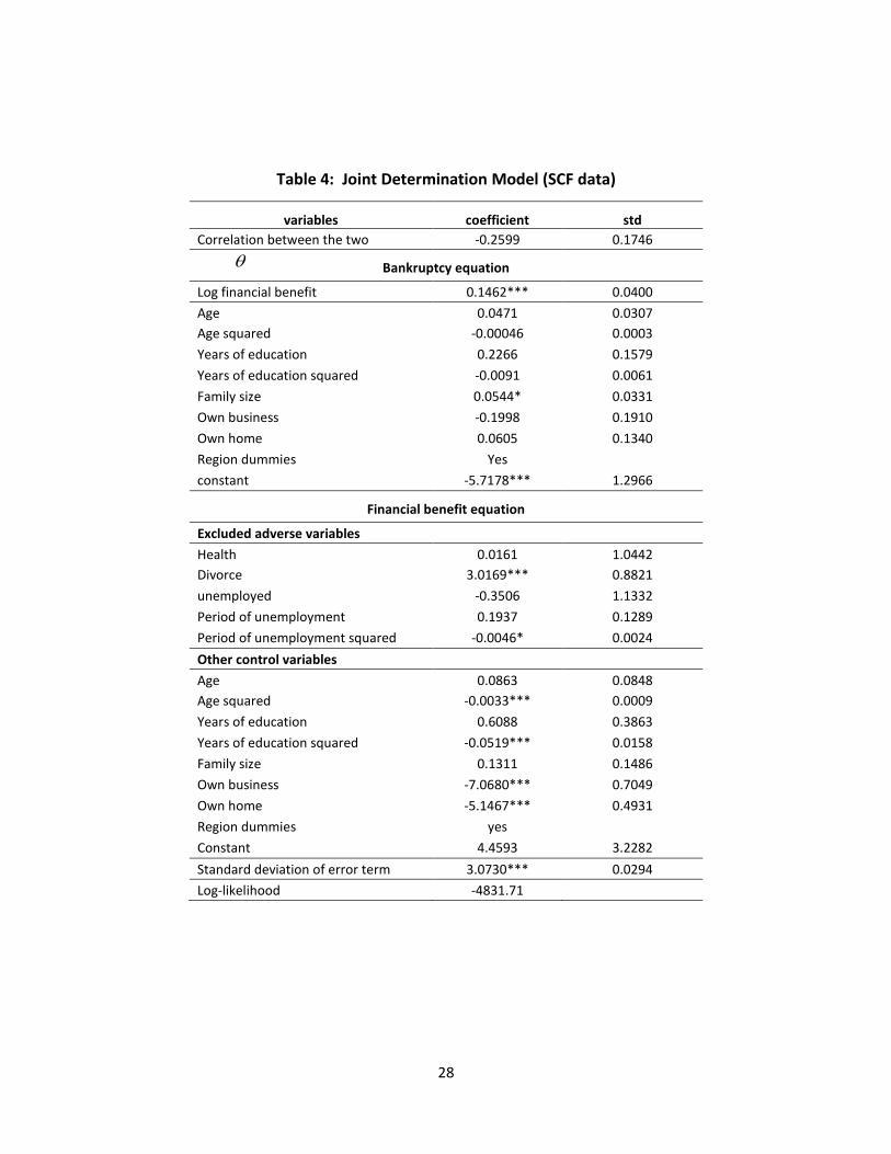
Estimation results are presented in tables 3 and 4.23 We find that using either PSID data

(table 3), or SCF data (table 4), the estimated parameter is not statistically different

from zero, consistent with non-strategic behavior.

At the same time, log financial benefit has a positive and highly significant effect on the

decision to file for bankruptcy in both datasets.

Both datasets confirm the view that adverse events may affect financial benefit. Results

using PSID data are presented in Table 3 and those with SCF data in Table 4. 24 Both

23

We apply a log transformation to financial benefit, because this variable exhibits a distribution that is

similar to log-normal but is left-censored at zero. In particular, we use log(financial benefit + $1). This is to

capture the characteristics of censored data at zero. The transformed variable is also left-censored at

zero. The result is also robust if the actual value of financial benefit is adopted.

20

show similar results, with some differences in terms of statistical significance. Intuitively,

health problems would lead to a larger amount of debt and thus a potentially higher

financial benefit (highly significant in PSID data, not in SCF). In the absence of divorce,

there is a greater chance of repaying higher levels of debt (due to joint earnings),

leading to lower probability of filing. Or there may be lower levels of debts, due to

greater production of services at home (in case one spouse is not working), leading to

lower financial benefit from filing.25 Conversely, conditional on divorce, financial benefit

may be higher (highly significant in SCF data, not in PSID). Moreover, greater financial

benefit may also be due to more joint (and individual) debts being discharged to give

both partners a fresh start after divorce. Transitioning into unemployment typically

lowers access to debt markets, lowering financial benefit from filing (highly significant in

PSID, not in SCF). Conditional on being unemployed, an increase in duration of

unemployment is more likely to imply utilizing existing debt lines more completely, or

increases in debts outstanding due to non-servicing of debt, both increasing financial

benefit. This increase may be tempered by more stringent conditions from creditors,

leading to an increasing and concave impact on financial benefit (highly significant in

PSID data, marginally significant in SCF).

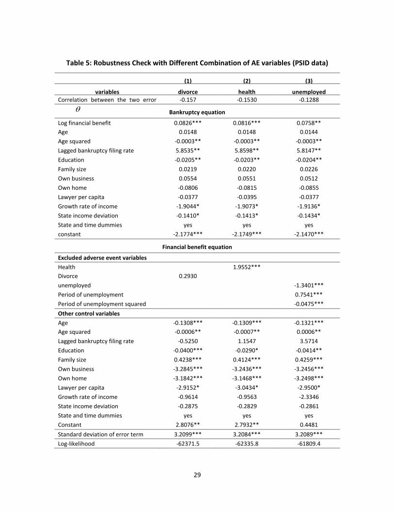
It is possible that not all adverse events have the same impact on filing behavior. For

example, a health shock may be less predictable than divorce, and may have a different

24

Since there is no available weak-IV test or Sargan test for the joint determination model, we run the

regression with two-stage-least-square to show the related statistics. For PSID, the F-statistic is 18.34,

which is greater than the critical value of 10, by rule of thumb. This rejects the null hypothesis that the

instruments are weak. The Sargan score is 5.898, with p-value of 0.21. So the over-identifying restriction is

valid. For SCF, the Anderson–Rubin (AR) statistic (chi-square=22.8), Kleibergen–Moreira Lagrange

multiplier (LM) test (chi-square=20.29), the conditional likelihood-ratio (CLR) test (statistic=21.39) all pass

the 5% significance, which rejects the null. The Sargan score is 6.53, which is 0.16 as of p-value. So we do

not reject the null hypothesis and the over-identifying restriction is valid.

25 According to Traczynski (2011), marriage is another kind of individual insurance against adverse shocks

through income sharing between partners; when the exemption level is high enough, people will choose

to file for bankruptcy instead of using marriage as their income protection.

21

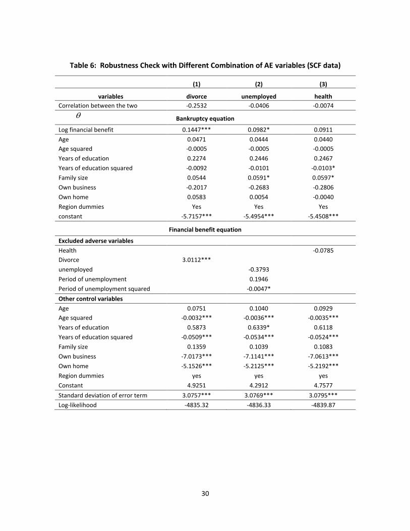
impact on filing behavior. Therefore, in principle, different adverse events could lead to

differing strategic behavior depending on type of adverse event. For robustness, we run

the joint determination model with different combinations of adverse events. The main

results are unchanged, as shown in Tables 5 and 6.

3.4 Interpretation

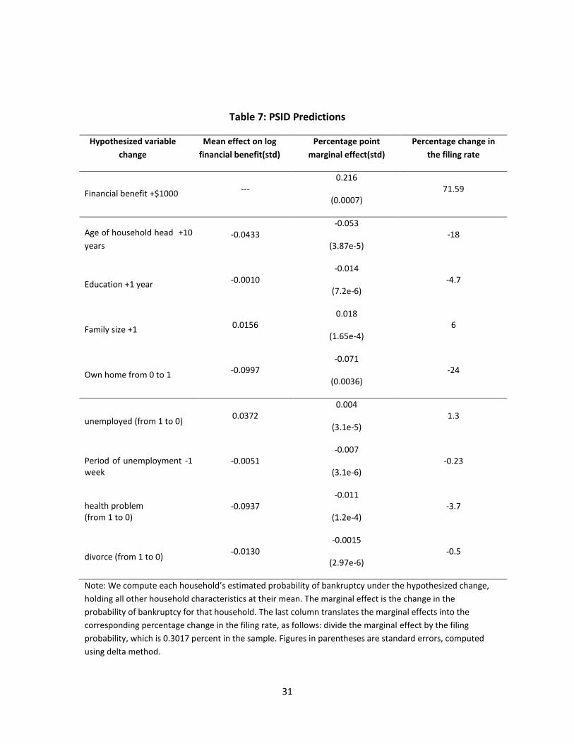
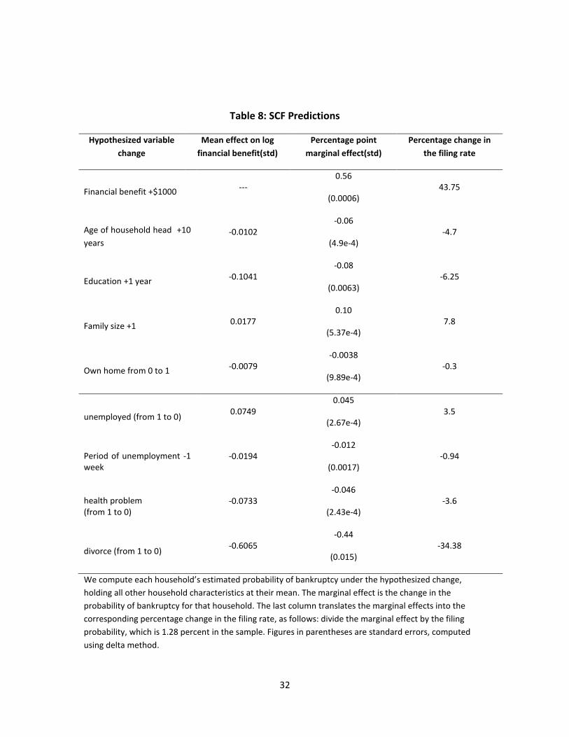
Tables 7 and 8 show how hypothetical changes in key variables affect financial benefit

from filing and probability of filing. Table 7 shows information for the joint

determination model using PSID data, whereas Table 8 shows the same information

using SCF data.

Suppose financial benefit from filing increases by $1,000 for each household.26 In this

case, the average filing probability is predicted to increase by 0.216 percentage points

(PSID data, Table 7) and by 0.56 percentage points (SCF data, Table 8). Given that filing

probability is 0.3017 percent (PSID data) and 1.28 percent (SCF data), an increase in

financial benefit of $1,000 predicts that bankruptcy filing rates would increase by 71.6

percent per year (using PSID data), and by 43.8 percent (using SCF data). Thus,

consistent with the basic theory outlined above, even with non-strategic behavior,

financial benefit can have a large effect on bankruptcy filings.27

We also present predictions for changes in some household characteristics, such as age

of head of household, education level, family size, and home ownership.

26

If negative, set the value to be zero.

27 Notice that the PSID sample has an average financial benefit of $1411 (Table 1), and a $1,000 change is

about 70 percent of this number. For the SCF a $1,000 change is about a 25 percent increase from the

mean of $3,991.

22

If age of head of the average household increases by 10 years, using equation (4), we

see that log financial benefit would decrease, on average, by 0.0433 (PSID data) and by

0.0102 (SCF), which would lead to 18.0 percent (PSID) and 4.7 percent (SCF) reduction in

annual bankruptcy filing rate.

If head of the average household receives one more year of education, the predicted

change in financial benefit is -0.001 (PSID) and -0.1041 (SCF). Bankruptcy filing rates

would decrease by 4.7 percent (PSID) and 6.25 percent (SCF).

If the average household adds one member, bankruptcy filing rate increases by 6.0

percent (PSID) and 7.8 (SCF) percent.

Home ownership has different effect in the two samples. If every household turns from

having no home to having at least one home, the bankruptcy filing rate using PSID data

is predicted to decrease by 24 percent (PSID) while the filing rate using SCF data is

predicted to drop only 0.3 percent. This might be due to the fact that SCF does not

release state information, and we might under-estimate the homestead exemption if

the state does not set a cap on homestead exemption.

Tables 7 and 8 present predictions based on changes in adverse event variables as well,

especially if adverse events did not occur. Broadly, except for unemployment, absence

of adverse events is predicted to decrease bankruptcy rates, as expected.

If head of an average household turned from being unemployed to having a job,

financial benefits are predicted to be higher on average, increasing predicted filing rates

by 1.3 percent (PSID) and 3.5 percent (SCF). Given that a head of household is

unemployed, if spell of unemployment is 1 week shorter, then financial benefits as well

as the bankruptcy filing rate is predicted to decrease by 0.23 percent (PSID) and 0.94

percent (SCF).

23

If the average household head turned from having health problem to not having health

problem, both predicted financial benefits and predicted bankruptcy filing rates would

decrease. The reduction in average bankruptcy rate is 3.7 percent (PSID) and 3.6 percent

(SCF), respectively.

Finally,’ suppose divorce did not occur, probability of bankruptcy filing is predicted to

decrease by 0.5 percent (PSID) and 34.4 percent (SCF).

4. Conclusion

Understanding the motivations of consumers to file for bankruptcy is central to the

design of appropriate policies to manage the number of filings. For example, if

consumers typically file strategically, and it is determined that filings are too high, then

policies to reduce filings could include, among others, those that tighten access to

bankruptcy courts, or make bankruptcy more expensive, perhaps by restricting access to

particular types of bankruptcy provisions, lowering exemptions, diverting more debtors

to longer repayment plans, lengthening minimum time between repeat filings, or

requiring debt management programs outside of bankruptcy. On the other hand, if

consumers typically file non-strategically, then policies to reduce bankruptcy filings

could include, among others, those that minimize the impact of adverse events, or

increase financial literacy for planning for such events.

This paper proposes a test to detect strategic or non-strategic behavior in bankruptcy

filings. The test is based on endogeneity or exogeneity of financial benefit and the

bankruptcy decision. The proposed test is more realistic than a simple estimation of the

sign of the coefficient on financial benefit and on adverse shocks. The test is partial in

that it cannot distinguish between strategic filing and a filing that appears to be

strategic due to non-strategic reasons. Nevertheless, test results are consistent with

24

non-strategic filing behavior, and rule out significant strategic behavior. The same

results hold in two different datasets.

The models used in this paper are simplified and by no means capture all relevant

aspects of the bankruptcy decision. Issues related to choosing a particular period to file

for bankruptcy, or to repeat interactions with credit markets, or to choice of bankruptcy

chapter, or to role of legal advertising, or to effects on supply of credit, or to effects on

work incentives, and so on are not considered here. (Some of these are the subject of

other papers, listed above.) It is possible to consider some of these issues here in a

reduced form by including parameters for expected gains and losses from delaying a

decision, or reduced access to credit markets, or utility penalties for default, and then

focusing on parameter values which make particular versions of the models more likely

to occur, but it is unclear if such additions would have additional applications given the

paucity of available data.

The results here can be viewed as providing an indication of some non-strategic

behavior in bankruptcy filings, rather than a definitive conclusion in favor of one

hypothesis or the other. For example, in addition to research supporting different

hypotheses, the reported surge in bankruptcy filings before the deadline of October 17,

2005 for the new bankruptcy law to go into effect suggests that other factors (perhaps

informational spillovers emerging from declining social stigma, or lawyer advertising)

are important as well. No doubt, additional work may yield additional testable

predictions, and additional research would be very welcome.

25

Table 1: Summary Statistics

Variables PSID data SCF data

Mean value

Standard deviation

Mean value

Standard deviation

Number of bankruptcy filings 254 55

Financial benefit $1,411 $10,523 $3,991 $26,001

Log(financial benefit +1) 1.64 3.24 1.94 3.69

Those file for bankruptcy 3.65 4.26 6.78 4.38

Log(unsecured debt+1) 3.85 3.94 4.35 4.45

Those file for bankruptcy 5.74 3.96 5.88 3. 96

Debts (if financial benefit>0) 9,329 31,800 9,549 38,318

Nonexempt assets(if financial benefit>0)

585 15,000 1,981 29,429

Household labor income $26,552 $32,672 $114,192 $602,833

Age of household head 44.19 15.96 49.84 16.52

Years of education of household head 12.43 5.10 13.74 2.90

Family size 2.90 1.55 2.65 1.44

Own home 0.59 0.49 0.70 0.46

Self employed/own business 0.11 0.31 0.25 0.44

Head is divorced 0.03 0.18 0.036 0.186

Head is unemployed 0.06 0.23 0.097 0.295

Weeks of unemployment of head 6.76 2.01 1.82 7.90

Head has health problem 0.07 0.26 0.04 0.19

ln(income) 8.17 4.76

Total number of observations 64,200 4,305

26

Table 2: Simple Probit Model

PSID data SCF data

without adverse event

variables

with adverse event variables

without adverse event

variables

with adverse event variables

financial benefit 0.00006*** (0.00001)

0.00006*** (0.00001)

0.00003*** (6.9e-6)

0.00003*** (7e-6)

financial benefit squared

-1.04e-9*** (4.04e-10)

-1.03e-9*** (3.99e-10)

-1.55e-10* (8.15e-11)

-1.61e-10** (8.2e-11)

lagged bankruptcy rate

5.95905** (2.67377)

5.62294** (2.68448)

household labor income

-4.98e-6*** (1.41e-6)

-4.12e-6*** (1.48e-6)

reduction in income -2.17e-6*** (5.92e-7)

-2.71e-7*** (7.34e-8)

age of household head

0.02917** (0.0137)

0.01846 (0.01306)

0.0486 (0.0339)

0.0281 (0.0302)

age squared -0.00048*** (0.00016)

-0.00036** (0.00015)

-0.00058 (0.00038)

-0.0003 (0.0003)

education -0.02981*** (0.01155)

-0.03879*** (0.01097)

0.0022 (0.0193)

-0.0125 (0.0198)

family size 0.03736** (0.01673)

0.03228* (0.01669)

0.0618* (0.0321)

0.0631* (0.0334)

own business 0.04037 (0.0918)

0.09489 (0.09147)

-0.3162 (0.1949)

-0.3321* (0.1858)

own home -0.1371* (0.07437)

-0.19982*** (0.06757)

-0.1122 (0.1435)

-0.1759 (0.1425)

lawyers per capita -0.7776 (0.74456)

-0.98042 (0.73636)

county unemployment rate

0.09337 (0.10457)

0.10714 (0.11386)

state income growth -2.39603** (1.19746)

-2.23304* (1.18386)

state income deviation

-0.12465 (0.08725)

-0.12976 (0.08821)

divorce

0.23206* (0.13196)

0.7627*** (0.1765)

period of unemployment

0.0134 (0.02435)

0.0047 (0.0053)

health problem

0.09265 (0.11733)

0.0359 (0.2980)

state fixed effects yes yes yes yes

year fixed effects yes yes no no

constant -2.3797*** (0.71384)

-2.23563*** (0.75997)

-3.5272*** (0.8701)

-3.2664*** (0.8059)

27

Table 3: Joint Determination Model (PSID data)

variables coefficient std err

Correlation between the two error terms -0.1402 0.1183

Bankruptcy equation

Log financial benefit 0.0786*** 0.0291

Age 0.0146 0.0114

Age squared -0.00026** .00013

Lagged bankruptcy filing rate 5.8113** 2.3557

Education -0.0204** 0.0083

Family size 0.0223 0.0145

Own business 0.0528 0.0804

Own home -0.0839 0.0574

Lawyer per capita -0.0376 0.6017

Growth rate of income -1.9152* 1.1194

State income deviation -0.1429* 0.0764

State and time dummies yes

constant -2.1588*** 0.4615

Financial benefit equation

Excluded adverse event variables

Health 1.9230*** 0.2287

Divorce 0.3550 0.3391

unemployed -1.3573*** 0.2645

Period of unemployment 0.7437*** 0.1970

Period of unemployment squared -0.0470*** 0.0124

Other control variables

Age -0.1338*** 0.0263

Age squared -0.00067** 0.00028

Lagged bankruptcy filing rate -3.7895 8.5598

Education -0.0306* 0.0169

Family size 0.4164*** 0.0401

Own business -3.2056*** 0.2267

Own home -3.2106*** 0.1331

Lawyer per capita -3.0452* 1.7055

Growth rate of income -2.2850 3.4461

State income deviation -0.2774 0.2114

State and time dummies yes

Constant 0.4705 1.4079

Standard deviation of error term 3.2073*** 0.0067

Log-likelihood -61774.312

28

Table 4: Joint Determination Model (SCF data)

variables coefficient std

Correlation between the two

errors

-0.2599 0.1746

Bankruptcy equation

Log financial benefit 0.1462*** 0.0400

Age 0.0471 0.0307

Age squared -0.00046 0.0003

Years of education 0.2266 0.1579

Years of education squared -0.0091 0.0061

Family size 0.0544* 0.0331

Own business -0.1998 0.1910

Own home 0.0605 0.1340

Region dummies Yes

constant -5.7178*** 1.2966

Financial benefit equation

Excluded adverse variables

Health 0.0161 1.0442

Divorce 3.0169*** 0.8821

unemployed -0.3506 1.1332

Period of unemployment 0.1937 0.1289

Period of unemployment squared -0.0046* 0.0024

Other control variables

Age 0.0863 0.0848

Age squared -0.0033*** 0.0009

Years of education 0.6088 0.3863

Years of education squared -0.0519*** 0.0158

Family size 0.1311 0.1486

Own business -7.0680*** 0.7049

Own home -5.1467*** 0.4931

Region dummies yes

Constant 4.4593 3.2282

Standard deviation of error term 3.0730*** 0.0294

Log-likelihood -4831.71

29

Table 5: Robustness Check with Different Combination of AE variables (PSID data)

(1) (2) (3)

variables divorce health unemployed Correlation between the two error

terms

-0.157 -0.1530 -0.1288

Bankruptcy equation

Log financial benefit 0.0826*** 0.0816*** 0.0758**

Age 0.0148 0.0148 0.0144

Age squared -0.0003** -0.0003** -0.0003**

Lagged bankruptcy filing rate 5.8535** 5.8598** 5.8147**

Education -0.0205** -0.0203** -0.0204**

Family size 0.0219 0.0220 0.0226

Own business 0.0554 0.0551 0.0512

Own home -0.0806 -0.0815 -0.0855

Lawyer per capita -0.0377 -0.0395 -0.0377

Growth rate of income -1.9044* -1.9073* -1.9136*

State income deviation -0.1410* -0.1413* -0.1434*

State and time dummies yes yes yes

constant -2.1774*** -2.1749*** -2.1470***

Financial benefit equation

Excluded adverse event variables

Health 1.9552***

Divorce 0.2930

unemployed -1.3401***

Period of unemployment 0.7541***

Period of unemployment squared -0.0475***

Other control variables

Age -0.1308*** -0.1309*** -0.1321***

Age squared -0.0006** -0.0007** 0.0006**

Lagged bankruptcy filing rate -0.5250 1.1547 3.5714

Education -0.0400*** -0.0290* -0.0414**

Family size 0.4238*** 0.4124*** 0.4259***

Own business -3.2845*** -3.2436*** -3.2456***

Own home -3.1842*** -3.1468*** -3.2498***

Lawyer per capita -2.9152* -3.0434* -2.9500*

Growth rate of income -0.9614 -0.9563 -2.3346

State income deviation -0.2875 -0.2829 -0.2861

State and time dummies yes yes yes

Constant 2.8076** 2.7932** 0.4481

Standard deviation of error term 3.2099*** 3.2084*** 3.2089***

Log-likelihood -62371.5 -62335.8 -61809.4

30

Table 6: Robustness Check with Different Combination of AE variables (SCF data)

(1) (2) (3)

variables divorce unemployed health

Correlation between the two

errors

-0.2532 -0.0406

-0.0074

Bankruptcy equation

Log financial benefit 0.1447*** 0.0982*

0.0911

Age 0.0471 0.0444 0.0440

Age squared -0.0005 -0.0005 -0.0005

Years of education 0.2274 0.2446 0.2467

Years of education squared -0.0092 -0.0101 -0.0103*

Family size 0.0544 0.0591* 0.0597*

Own business -0.2017 -0.2683 -0.2806

Own home 0.0583 0.0054 -0.0040

Region dummies Yes Yes Yes

constant -5.7157*** -5.4954*** -5.4508***

Financial benefit equation

Excluded adverse variables

Health -0.0785

Divorce 3.0112***

unemployed -0.3793

Period of unemployment 0.1946

Period of unemployment squared -0.0047*

Other control variables

Age 0.0751 0.1040 0.0929

Age squared -0.0032*** -0.0036*** -0.0035***

Years of education 0.5873 0.6339* 0.6118

Years of education squared -0.0509*** -0.0534*** -0.0524***

Family size 0.1359 0.1039 0.1083

Own business -7.0173*** -7.1141*** -7.0613***

Own home -5.1526*** -5.2125*** -5.2192***

Region dummies yes yes yes

Constant 4.9251 4.2912 4.7577

Standard deviation of error term 3.0757*** 3.0769*** 3.0795***

Log-likelihood -4835.32 -4836.33 -4839.87

31

Table 7: PSID Predictions

Hypothesized variable

change

Mean effect on log

financial benefit(std)

Percentage point

marginal effect(std)

Percentage change in

the filing rate

Financial benefit +$1000 --- 0.216

(0.0007) 71.59

Age of household head +10

years -0.0433

-0.053

(3.87e-5) -18

Education +1 year -0.0010 -0.014

(7.2e-6) -4.7

Family size +1 0.0156 0.018

(1.65e-4) 6

Own home from 0 to 1 -0.0997 -0.071

(0.0036) -24

unemployed (from 1 to 0) 0.0372

0.004

(3.1e-5) 1.3

Period of unemployment -1 week

-0.0051 -0.007

(3.1e-6) -0.23

health problem (from 1 to 0)

-0.0937 -0.011

(1.2e-4) -3.7

divorce (from 1 to 0) -0.0130

-0.0015

(2.97e-6) -0.5

Note: We compute each household’s estimated probability of bankruptcy under the hypothesized change,

holding all other household characteristics at their mean. The marginal effect is the change in the

probability of bankruptcy for that household. The last column translates the marginal effects into the

corresponding percentage change in the filing rate, as follows: divide the marginal effect by the filing

probability, which is 0.3017 percent in the sample. Figures in parentheses are standard errors, computed

using delta method.

32

Table 8: SCF Predictions

Hypothesized variable

change

Mean effect on log

financial benefit(std)

Percentage point

marginal effect(std)

Percentage change in

the filing rate

Financial benefit +$1000 --- 0.56

(0.0006) 43.75

Age of household head +10

years -0.0102

-0.06

(4.9e-4) -4.7

Education +1 year -0.1041 -0.08

(0.0063) -6.25

Family size +1 0.0177 0.10

(5.37e-4) 7.8

Own home from 0 to 1 -0.0079 -0.0038

(9.89e-4) -0.3

unemployed (from 1 to 0) 0.0749

0.045

(2.67e-4) 3.5

Period of unemployment -1 week

-0.0194 -0.012

(0.0017) -0.94

health problem (from 1 to 0)

-0.0733 -0.046

(2.43e-4) -3.6

divorce (from 1 to 0) -0.6065

-0.44

(0.015) -34.38

We compute each household’s estimated probability of bankruptcy under the hypothesized change,

holding all other household characteristics at their mean. The marginal effect is the change in the

probability of bankruptcy for that household. The last column translates the marginal effects into the

corresponding percentage change in the filing rate, as follows: divide the marginal effect by the filing

probability, which is 1.28 percent in the sample. Figures in parentheses are standard errors, computed

using delta method.

33

References

Adams, W., L. Einav, and J. Levin (2009): “Liquidity constraints and imperfect

information in subprime lending,” American Economic Review, 99(1), 49-84

Arabmazar, A. and P. Schmidt (1982): “An investigation of the robustness of the Tobit

estimator to non-normality,” Econometrica, 50, 1055-64.

Araujo, A. and M. Pascoa (2002): “Bankruptcy in a model of unsecured claims,”

Economic Theory, 20(3), 455-481.

Athreya, K. (2005): “Equilibrium Models of Personal Bankruptcy: A Survey,” Federal

Reserve Bank of Richmond Economic Quarterly, 91(2), 73-98.

Ausubel, L. M. (1991): “The failure of competition in the credit card market,” American

Economic Review,” 81(1), 50-81.

Ausubel, L. M. (1997): “Credit card defaults, credit card profits, and bankruptcy,”

American Bankruptcy Law Journal, 71, 249-270.

Berkowitz, Jeremy, and Richard Hynes (1999): "Bankruptcy Exemptions and the Market

for Mortgage Loans," Journal of Law and Economics, 42(2), 809-830

Crow, E. L., and K. E. Shimizu (1988): Lognormal Distributions: Theory and Applications,

Dekker, New York.

Domowitz, Ian, and Thomas L. Eovaldi (1993): "The Impact of the Bankruptcy Reform Act

of 1978 on Consumer Bankruptcy," Journal of Law and Economics, 36(2), 803-

835

Domowitz, P. J. and R. L. Sartain (1999): “Determinants of the consumer bankruptcy

decision,” Journal of Finance, 54(1), 403-420.

Dubey, P., J. Geanakoplos, and M. Shubik (2005): “Default and punishment in general

equilibrium,” Econometrica, 73(1), 1-37.

Elias, S., A. Renauer, and R. Leonard (1999): How to file for chapter 7 bankruptcy, Nolo

Press, 8th edition

34

Eaton, J., and M. Gersovitz (1981): “Debt with Potential Repudiation: Theoretical and

Empirical Analysis,” Review of Economic Studies, 48(2), 289-309

Fan, W. and M. J. White (2003): “Personal bankruptcy and the level of entrepreneurial

activity,” Journal of Law and Economics, 46(2), 543-568.

Fay, S., E. Hurst, and M. J. White (2002): “The household bankruptcy decision,”

American Economic Review, 92(3), 706-718.

Gan, L., M. Hurd, and D. McFadden (2005): “Individual subjective survival curves,” in D.

Wise ed., Analyses of Economics of Aging, The University of Chicago Press, 2005:

377-411.

Gan, L. and T. Sabarwal (2005): “A Simple Test of Adverse Events and Strategic Timing

Theories of Consumer Bankruptcy,” NBER Working Paper Series, No. 11763,

November

Gan, Li, Feng Huang, and Adalbet Mayer (2010). “A simple test of private information in

the insurance markets with heterogeneous insurance demand.” NBER Working

Paper Series, No 16738.

Gan, L., and Roberto Mosquera (2008). “ An empirical study of the credit market with

unobserved consumer types. “ NBER Working Paper Series, No 13873.

Geanakoplos, J., and W. Zame (2007): “Collateralized Asset Markets,” mimeo.

General Accounting Office (1998): “Personal bankruptcy: the credit research center

report on debtors’ ability to pay,” GAO/GGD-98-47.

General Accounting Office (1999): “Personal bankruptcy: a report on petitioner’s ability

to pay,” GAO/GGD-99-103.

Gropp, Reint E., John Karl Scholz, and Michelle J. White. (1997): "Personal Bankruptcy

and Credit Supply and Demand." Quarterly Journal of Economics 112:217–52.

Lefgren, Lars and Frank McIntyre (2009), "Explaining the Puzzle of Cross-State

Differences in Bankruptcy Rates," Journal of Law and Economics, 52(2), 367-393

Li,Wenli, Michelle J. White, and Ning Zhu. (2011): "Did Bankruptcy Reform Cause

Mortgage Defaults to Rise?" American Economic Journal: Economic Policy

3(4):123–47.

35

Greenhalgh-Stanley, Nadia and Shawn Rohlin (2013): "How Does Bankruptcy Law Impact

the Elderly's Business and Housing Decisions?" Journal of Law and Economics,

56(2), 417-451

Gross, T., M.J.Notowidigdo, and J. Wang (2012): “Liquidity Constraints and Consumer

Bankruptcy: Evidence From Tax Rebates,” NBER Working Paper Series, No. 17807

Gross and Souleles (2002):"Do Liquidity Constraints And Interest Rates Matter For

Consumer Behavior? Evidence From Credit Card Data," The Quarterly Journal of

Economics, 117(1), 149-185

Han, S. and G. Li (2009): “Household borrowing after personal bankruptcy,” Working

paper, Finance and Economics Discussion Series, 2009-17

Hoelle, M. (2009): “A Simple Model of Bankruptcy in General Equilibrium,” Working

paper, University of Pennsylvania

Kennickell, A., M. Starr-McCluer, and B. J. Surette (2000). “Recent change in U.S. family

finances: results from the 1998 Survey of Consumer Finances.” Federal Reserve

Bulletin, Division of Research and Statistics, Federal Reserve Board

Livshits, I, J. Macgee, and M. Tertilt (2007): “Consumer bankruptcy: a fresh start,”

American Economic Review, 97(1), 402-418

Livshits, I, J. Macgee, and M. Tertilt (2010): “Accounting for the rise in consumer

bankruptcies,” American Economic Journal: Macroeconomics, 2(2): 165-93

Luckett, C. A. (2002): “Personal Bankruptcies,” The Impact of Public Policy on Consumer

Credit, 69-108

Mansi, Sattar A., William F. Maxwell, and John K. Wald (2009): "Creditor Protection Laws

and the Cost of Debt," Journal of Law and Economics, 52(4), 701-717

Modica, M., A. Rustichini, and J. M. Tallon (1999): “Unawareness and bankruptcy: a

general equilibrium model,” Economic Theory, 12(2), 259-292.

Musto, D. K. (2004): “What happens when information leaves a market? Evidence from

post bankruptcy consumers,” Journal of Business, 77(4), 1-24

Powell, J. (1984): “Least absolute deviations estimation for the censored regression

model,” Journal of Econometrics, 25: 303-325.

36

Sabarwal, T. (2003): “Competitive equilibria with incomplete markets and endogenous

bankruptcy,” Contributions to Theoretical Economics, 3(1), Art. 1.

Stanley, D. T., and M. Girth (1971): Bankruptcy: problem, process, reform. Brookings

Institution, Washington DC

Sullivan, T. A., E. Warren, and J. L. Westbrook (1989): As we forgive our debtors. Oxford

University Press

Sullivan, T. A., E. Warren, and J. L. Westbrook (1994): “Consumer debtors ten years

later: a financial comparison of consumer bankrupts, 1981-1991,” American

Bankruptcy Law Journal, 68, 121-154.

Sullivan, T. A., E. Warren, and J. L. Westbrook (2000): The Fragile Middle Class. Yale

University Press

Traczynski, J. (2011): "Divorce Rates and Bankruptcy Exemption Levels in the United

States," Journal of Law and Economics 54(3), 751-779

Warren, C. (1935): Bankruptcy in United States history. Harvard University Press

White, M. J. (1987): “Personal bankruptcy under the 1978 bankruptcy code: an

economic analysis,” Indiana Law Journal, 63(1), 1-53.

White, M. J. (1998): “Why don’t more households file for bankruptcy?” Journal of Law,

Economics, and Organization, 14(2), 205-231.

Zame, W. (1993): “Efficiency and the role of default when security markets are

incomplete,” American Economic Review, 83(5), 1142-1164.