Strategic Timing of IPO and Disclosure - a Dynamic

Model of Multiple Firms∗

Cyrus Aghamolla†

Graduate School of Business

Columbia University

Ilan Guttman‡

Stern School of Business

New York University

May 2015

Preliminary Draft

Abstract

We study a dynamic game between multiple firms who decide when to disclose their

private information and sell the firm (IPO) or a project. Firms privately learn their

type and are uncertain as to a common factor to all the firms. The common factor

follows a stochastic mean-reverting process and is revealed only following an IPO. We

characterize the unique symmetric threshold equilibrium and show that there is always

a positive amount of delay in going public. Firms consider the trade-off between the

direct costs of delaying the IPO and the value of the real option from delaying the

IPO, which stems from potentially learning the common factor. The model predicts

that the number of expected IPOs in the second period is increasing in the realization

of the common factor in the first period, so that we expect clustering of IPOs following

a successful IPO. We suggest several empirical predictions regarding firm equilibrium

strategies and the timing of IPOs.

∗We are grateful to seminar participants at Baruch, Carnegie Mellon, Columbia, NYU, and Warwick.†E-mail: caghamolla18@gsb.columbia.edu.‡E-mail: iguttman@stern.nyu.edu.

1

1 Introduction

In 2014, U.S. public equity markets saw more initial public offerings (IPOs) than in any year

since the 2000 dot-com boom. The recent wave of IPOs has been especially interesting given

the initial diffi culty the market had in evaluating firms in new industries, particularly social

media and cloud computing. As one commentator noted during the 100% price increase on

the initial day of trading for LinkedIn: "New internet companies based on new and innovative

technologies are more diffi cult to value."1 In new industries with uncertain fundamentals,

firms that had received higher than expected valuations led to further, more immediate public

offerings by other firms within the same industry, whereas firms who received less favorable

valuations delayed the IPO plans of other similar firms. For example, consider the pioneer

firm to go public in the new social media industry, Facebook. The price fall that ensued

Facebook’s IPO allegedly pushed back the offering of Twitter for several months. Twitter

went public only when the market was better able to assess Facebook’s value, in a very

favorable way, which resulted in a tremendous price increase around the IPO. The ability to

see the market sentiment before going public provide firms an advantage in choosing their

disclosure time.2

We seek to study such behavior in a strategic game of disclosure/IPO by multiple firms,

in which each firm strategically chooses when to disclose its private information and go public

(or sell a project). In particular, we study the following three-period multi-firm/entrepreneur

setting. The value of each firm/project is determined by two components: an idiosyncratic

component, which we refer to as the firm’s type, and a common component which affects all

firms in the industry/economy who consider an IPO. The first ingredient of our model is that,

given all else equal, each firm’s manager/entrepreneur wants to sell the firm/project as early

as possible. This assumption could reflect that delaying IPO leads to, for example: forgoing

profitable investment and expansion opportunities, potential loss of market power relative

to competitors and hence reduced payoff, the costs of debt that is used to finance projects

or operations, or even the tendency of a firm’s idiosyncratic component to mean-revert. To

1"Wall Street ’mispriced’LinkedIn’s IPO." Financial Times, March 30, 2011.2Several other firms, such as Kayak, have been reported to delay their IPO dates specifically because of

the market reaction to the Facebook IPO. See "Did IPO damage Facebook brand?", CBS Money Watch,June 6, 2012.

2

capture this time preference, we assume that firms/managers discount the payoff of future

payoff from selling the firm/project. The second ingredient of our model pertains to the

common factor, which can capture the state of nature, the state of the economy/industry,

or market sentiment. The state of nature is assumed to follow a mean-reverting stochastic

process. The state variable can be common to firms only within a specific industry, or to

all firms.3 Bessembinder et al. (1995) found that all the markets they examined are charac-

terized by mean-reversion, where there is substantial variation across industries in terms of

the reversal rates. The state variable can also be thought of as reversal of macroeconomic

shocks, as evidenced by Bloom (2009) and Bloom et al. (2014).

The state of nature is not observable, unless at least one of the firms goes public. As part

of the IPO process, the market learns and forms an opinion about the new technology or the

market conditions (captured by the state of nature) and reveals this information through

the pricing of the IPO. If no firm goes public, the state of nature is not revealed, e.g., had

Facebook not gone public in May 2012, there would have been a much greater uncertainty

about the market’s perception of the value and potential of the social media industry.

The mean reverting nature of the common factor gives rise to a real option from delaying

the IPO in the first period. In case a firm delays its IPO and another firm goes public, the

state of nature in the first period is revealed. If the realization of the state of nature in the

first period is suffi ciently low the firm is better off further delaying the IPO to the third

period. The reason is that while the state is expected to be low also in the second period,

it is expected to further revert to the mean in the third period, i.e. the state is expected to

increase between the second and the third period. However, if the realization of the state of

nature in the first period is suffi ciently high, the firm finds it more profitable to go public in

the second period. When deciding whether to IPO in the first period, the firm considers the

trade-off between the direct costs of delaying the IPO and the benefit from the value of the

real option from delaying the IPO4. The firm considers the probability that the other firms

3There is evidence that firms in different industries have different market sentiments, and that IPOswithin an industry share similar one-day returns and similar average returns. For example, technology IPOsperformed very well in 2014, whereas bank IPOs often failed to meet their price range. See "Bank IPO FallsShort of Target Price Range," Wall Street Journal, September 24, 2014.

4When firms go through an IPO they are required to disclose information, as part of the IPO prospectus.We will be using IPO and disclosure interchangeably throughout the paper.

3

will disclose and IPO in the first period; if no other firm goes public in the first period, the

state of nature will not be revealed and the option value will not be realized. This introduces

strategic interaction between firms, as the disclosure/IPO strategy of one firm affects the

payoff and the optimal strategy of the other firms.

We analyze the above setting and show that there exists a unique symmetric equilibrium.

In equilibrium, each firm follows a threshold strategy in each period. In particular, each firm

goes public in the first period if and only if the realization of its idiosyncratic component

(hereafter the firm’s type) is suffi ciently high.5 If there was no IPO by any firm in the first

period then the first-period state of nature is not revealed, and hence, all firms go public in

the second period (as the game ends in the third period). If at least one firm went public

in the first period then a firm that did not IPO in the first period goes public in the second

period only if the realization of the first-period state was suffi ciently high. The realization

of the first-period state of nature below which a firm delays the IPO in the second period is

lower the higher the firm type is. Low-type firms are thus comparatively more inclined to

delay the IPO not only in the first period, but in the second period as well. The reason is

two-fold: (i) the cost of delay due to the discount is comparatively lower for low-type firms,

and (ii) the value of the real option from delaying the IPO in the first period is decreasing

in a firm’s type.

Several interesting insights and empirical predictions emerge from this analysis. There is

always a positive amount of delay of IPO in equilibrium, where suffi ciently high type firms

do not delay. In general, the model predicts that the higher a firm’s type, the earlier it will

disclose and go public, as higher type firms exhibit higher discounting costs and lower value

of the real option from delaying the IPO.

If no firm went public in the first period, we expect clustering of IPOs in the second

period.6 If there was at least one IPO in the first period, the expected number of IPOs

in the second period is increasing in the first-period realization of the state. That is, we

5In an extension of the model we study a setting in which firm type is bounded from above and show thatfor this setting the symmetric equilibrium may not be unique. In particular, we show that, for suffi cientlylow discount factors, there may also exist equilibria in which one firm always goes public in the first periodand the other firms never IPO in the first period.

6For simplicity, we study a three period setting, in which firms that did not IPO by the end of the secondperiod, do so in the third and last period. In a setting with more than three periods, there will be somedelay of IPOs in the second period, even if no firm went public in the first period.

4

expect clustering of IPOs in the second period following a successful IPO in the first period,

and fewer IPOs (or none) if the state of nature in the first period turned out to be low.

We find that the threshold level in each period is decreasing in the discount factor, since

for higher discount factor delaying the IPO is more costly and also the value of the real

option from delaying is lower. The variance of the state of nature affects the first-period

threshold but does not affect the second-period threshold. In particular, an increase in the

variance of the state of nature increases the option value from delaying the IPO due to

the increased volatility in the realization of the state, and hence increases the first-period

threshold. However, the second-period threshold is unaffected by the variance of the state

since firms/entrepreneurs are risk-neutral and at the second period there is no real option

from delaying the IPO. The reversal rate of the state variable has a less straightforward effect

on the threshold levels in both the first and the second period. For low levels of reversal

rate both periods’thresholds are increasing in the reversal rate where for higher levels both

period’s thresholds are decreasing in the reversal rate. The intuition is as follows. When the

reversal is full (that is, when state of nature is iid over time), the value of the real option

from learning the realization of the state in the first period is zero, since the states in the

second and third periods are independent of the first period’s state. At the other extreme,

as the reversal rate goes to zero, the process of the state variable converges to a random

walk. In such case, there is no reversal and the only value the real option may have is when

the realized state is suffi ciently low, such that the overall value of the firm is negative, and

hence delaying a negative payoff is beneficial.

The problem we investigate is practically relevant as the strategic timing of IPOs is a

veritable concern among firms. Indeed, firms typically delay their offering dates due to unfa-

vorable market sentiment (e.g., the case of Virtu who delayed its IPO due to dissatisfaction

over flash-trading7). Numerous empirical papers also provide evidence of the strategic tim-

ing of IPOs, e.g., Lougran, Ritter, and Rydqvist (1994), Lerner (1994), Pagan, Panetta,

and Zingales (1998) which document that IPO volume is higher following increase in market

7"For Virtu IPO, Book Prompts a Delay." The Wall Street Journal, April 3, 2014. The timing is aserious concern for firms: "Analysts said Virtu had little choice but to postpone the offering. ’The timingcouldn’t be worse,’said Pat Healy, CEO of Issuer Advisory Group LLC, which advises companies on goingpublic."

5

valuations.

The two papers perhaps most closely related to our study are Persons andWarther (1997)

and Alti (2005). Persons and Warther (2005) develop a model of financial innovation among

several firms who may move sequentially. Each firm observes the noisy cash flow returns of

firms who have already adopted the innovation and accordingly decides whether to adopt the

innovation. They generate "booms" in the adoption of the new technology, as each additional

firm that adopts the innovation may lead to another firm’s subsequent adoption. However, a

fundamental assumption in their model is that it is common knowledge which firms benefit

the most from the adoption of the technological innovation, and correspondingly, the firms

adopt the technology in a predetermined order, beginning with the firm that benefits the

most. This would be equivalent to the model here where each firms’idiosyncratic component

was commonly known, the state of nature does not follow a mean-reversion process and

adoption of the innovation increases the precision of the beliefs about the profitability of

the innovation. Likewise, Alti (2005) develops a model of information spillover in an IPO

setting, where information asymmetry decreases following an IPO, which consequently lowers

the cost of going public for the other firms. The cost of going public is due to adverse pricing

by the market in a second price auction in the presence of informed trader. The common

component among firms is the cash flow generated in the period of IPO, which is assumed

to be identical to all firms (and not mean-reverting). The support of per-period cash flow,

however, is assumed to be binary and unchanging.

Several other papers consider optimal IPO timing and IPO waves. Pastor and Veronesi

(2003) model the strategic timing of an IPO as an inventor who faces a problem analogous

to an American call option. The inventor can exercise the option to capitalize on abnormal

profits, but sacrifices the possibility that market conditions may worsen to cover the initial

investment. As here, their model relies heavily on market conditions for the timing of the

IPO, however, our model incorporates strategic interaction between firms that affects the

timing of IPOs. A number of other papers look at the strategic timing of IPOs. He (2007)

considers a game between investment banks and investors to generate high first day returns

during periods of high IPO volume. Chemmanur and Fulghieri (1999) models IPO timing as a

trade-off between selling the firm to a risk-averse venture capitalist at a discount or through

6

the loss in informational advantage from going public. Benninga, Helmantel, and Sarig

(2005) model the decision to go public as a trade-off between diversification and the private

benefits of control. They generate IPO waves during periods when expected cash flows are

high. Our model differs from these three as they are all single-firm models, whereas we are

principally interested in the strategic interaction between firms and the resulting clustering

effects. Indeed, a multi-firm setting of IPOs where firms’strategies are interdependent has

not been examined in the context of IPO waves in the extant literature.

Our model varies from the literature on dynamic voluntary disclosure (e.g., Dye and

Sridhar (1995), Acharya, DeMarzo, and Kremer (2011), Guttman, Kremer, and Skrzy-

pacz (2014)) in three ways: (i) in our setting there is no uncertainty about whether the

firm/entrepreneur is endowed with private information, (ii) in our setting the entrepreneur

is only concerned with the firm’s value in the period of disclosure and IPO, and (iii) in our

setting there are multiple firms/entrepreneurs whose decisions are interrelated.8

The following section presents the setting of the model and section three analyzes the

equilibrium. Section four examines comparative statics and offers empirical predictions.

Section five studies an extension of the model in which the support of the firms’ type is

bounded from above and the final section concludes. Proofs are relegated to the Appendix,

unless otherwise stated.

2 Model Setup

We study a setting with three periods, t ∈ 1, 2, 3, and N ≥ 2 firms. A firm’s value

is a function of an idiosyncratic component and the value of a common factor. Prior to

t = 1, each firm’s manager/entrepreneur privately observes the idiosyncratic component

of her firm’s value or project, θi, which is the realization of a random variable θ with a

cumulative density G (θ) and probability density function g (θ). We will often refer to θi as

the type of firm i. The support of θ is [0,∞) and g (θ) is positive over the entire support

of θ.9 For all i 6= j the idiosyncratic components, θi and θj, are independent. We constrain

8The latter feature is present in Dye and Sridhar (1995).9We later study the case in which the support of θ is bounded from above, i.e., θ ∈ [0, θ] and show that

the symmetric equilibrium that we characterize in the current section still holds. However, when the support

7

θ to be non—negative since this simplifies the analysis, however, the results would not be

qualitatively affected with negative firm values10. Firms’managers/owners are assumed to

be risk-neutral. Every firm manager must IPO the firm (or sell the project) in one of the

periods, while as part of the IPO the manager discloses the private type, θi. Disclosure of

the type is credible and costless. The managers are assumed to maximize the firm’s market

price at the time of disclosure. For example, the manager/owner may want to sell (IPO)

the firm and needs to make a disclosure at the selling time (IPO). The firm’s price at the

time of the IPO depends on investors’beliefs about both the idiosyncratic component, θi,

as well as on the state of nature at the time of the IPO, which is denoted by st. The market

price at time τ of firm i that discloses θi at t = τ equals investors’expectation of θi + sτ

given all the available information at t = τ , which we denote by Ωτ . Every firm’s manager

has a time preference (discount) which is denoted by r, such that the expected utility of the

owner/manager of firm i from going public and disclosing θi at t = τ is given by:

ui,τ =E (θi + sτ |Ωτ )

(1 + r)τ−1.

Discounting is meant to capture the costs associated with delaying the sale of a project or

shares. Such cost could be due, for example: costs of debt, the cost from forgoing investment

and acquisition opportunities due to lack of financing, and the decrease in profitability due

to increase in competition. The state of nature in each period, st, is ex-ante unobserved,

however, upon IPO by at least one of the firms, all firms learn st at the end of the period

in which an IPO took place11. We assume that the state of nature follows a mean-reverting

AR(1) process of the form:

st = γst−1 + εt,

of θ is bounded from above, there exists another equilibrium in which one firm always discloses at t = 1 andall the other firms do not disclose (or follow a disclosure threshold).

10With negative values, firms would be compelled to delay disclosure since discounting works to improvethe firm’s payoff. We eliminate this case to not confound the results.

11A possible extension is to assume that the market obtains a noisy signal of the state of nature when adisclosure is made. The more firms disclose the higher the precision of the market inference about the stateof nature.We believe this is a realistic assumption that should not make a qualitative difference. However, it will

complicate the analysis as the indifference condition will have to take into account all the permutations oftypes that will disclose at t = 1 and the corresponding option value - which depends on the variance of thesignal about s1, which in turn depends on the number of firms that disclose at t = 1.

8

where γ ∈ (0, 1) and εt ∼ N (0, σ2) with a cumulative distribution function F (·) and density

function f (·) 12. The initial state is given by s0 = 0, and so the first period’s state is given

by s1 = ε1. Hence, the state of the economy in the first period is simply a mean-zero error

term.

The mean-reversion property of the state of nature, which is one of the central assump-

tions in our model, is taken exogenously. However, both the empirical and theoretical litera-

ture provide ample support for mean reversion of both specific stock returns (e.g., Fama and

French (1988) and Poterba and Summers (1988)) and of macroeconomic measures, such as

stock market indices (e.g., Richards (1997)). Mean reversion can be motivated by fully ratio-

nal settings (e.g., Cecchetti, Lam and Nelson 1990) and high-order beliefs in an overlapping

generation (as in Allen, Morris, and Shin (2006))13, or by behavioral explanations such as

investors sentiment and limits to arbitrage (e.g., Baker and Wurgler (2006)). Mean reversion

of the state of nature in our setting can also be motivated by dynamic competition in the

market that affects the common factor. For example, when the state of nature, which may

represent the perceived profitability of the relevant technology, is high in the first period,

firms have an incentive to increase their activity in this market/technology, which in return

will decrease the profitability in this market. A symmetric argument applies to a low state

of nature.

The sequence of events in the game is as follows: Prior to t = 1 all managers/firms

privately observe the idiosyncratic component of their firm value, θi. In t = 1, each firm

decides weather to IPO in this period. Firms make their decisions simultaneously. If at

least one firm made an IPO the state of nature at t = 1, s1, is publicly observed and firms

that disclosed and IPO receive their market valuation. Those firm managers receive their

corresponding payoff and the remainder of the game is irrelevant for them. At period t = 2,

all firms that did not IPO at t = 1 make a disclosure/IPO decision. If at least one firm IPO

12Alternatively, we could have the variance of the error decreasing in each period to reflect the market’sability to better evaluate the firm in later periods. This would not affect the results since firms are assumedto be risk neutral and only the variance level in the first period, which affects the value of the real optionfrom delaying disclosure, is consequential.

13Mean reversion due to high-order beliefs in an Allen, Morris and Shin setting is as follows. Since in thefirst period the private signals are underweighting in the price formation it gives rise to a biased investorsbeliefs about the intrinsic value. As time goes by, on expectation, this bias decreases and the price convergesto the unbiased mean.

9

at t = 2 the realization of the state of nature, s2 is publicly revealed. The market valuation

of firms that IPO at t = 2 is determined and manager’s of those firms receive their payoff.

Finally, at t = 3, which is the last period of the game, all firms that have not yet gone

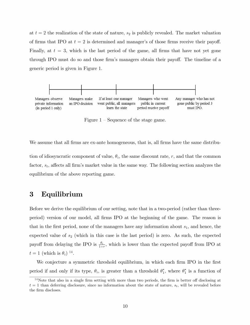
through IPO must do so and those firm’s managers obtain their payoff. The timeline of a

generic period is given in Figure 1.

Figure 1 —Sequence of the stage game.

We assume that all firms are ex-ante homogeneous, that is, all firms have the same distribu-

tion of idiosyncratic component of value, θi, the same discount rate, r, and that the common

factor, st, affects all firm’s market value in the same way. The following section analyzes the

equilibrium of the above reporting game.

3 Equilibrium

Before we derive the equilibrium of our setting, note that in a two-period (rather than three-

period) version of our model, all firms IPO at the beginning of the game. The reason is

that in the first period, none of the managers have any information about s1, and hence, the

expected value of s2 (which in this case is the last period) is zero. As such, the expected

payoff from delaying the IPO is θi1+r, which is lower than the expected payoff from IPO at

t = 1 (which is θi) 14.

We conjecture a symmetric threshold equilibrium, in which each firm IPO in the first

period if and only if its type, θi, is greater than a threshold θ∗1, where θ

∗1 is a function of

14Note that also in a single firm setting with more than two periods, the firm is better off disclosing att = 1 than deferring disclosure, since no information about the state of nature, st, will be revealed beforethe firm discloses.

10

all the parameters of the model (the distributions of the types, the distribution of the state

of nature and the degree of mean-reversion, the number of firms, and the discount factors).

At t = 2, if firm j 6= i went public at t = 1, firm i IPO if and only if θi > θ∗2 (si). Note

that if there were no IPOs at t = 1, then this reduces to the two-period setting mentioned

above, and hence, all firms IPO in t = 2. Given that there is positive probability of IPO by

at least one other firm in the first period, firm i has a real option from delaying the IPO at

t = 1, hoping to observe s1 at the end of period 1. Upon observing the state of nature, s1,

for suffi ciently negative realizations of the state of the economy, the firm rather delay the

IPO until t = 3, as the state of nature follows a mean-reverting process, such that the state

of nature is expected to increase towards zero at t = 3.

In light of the above behavior in period 2, firms at t = 1 have to take into consideration

the trade-off between the benefit from the above real option and the cost of delaying the

IPO. The cost of delaying, due to the discount factor r, increases in the firm’s type, θi.

Moreover, as we show below, the value of the real option from delaying the IPO at t = 1

is decreasing in the firm’s type, θi. As such, both of the above effects work in the same

direction. That is, any firm follows a threshold strategy at t = 1 such that, for realizations

of θi that are suffi ciently high, the manager prefers to IPO at t = 1, whereas for lower

realizations the manager is better off delaying the IPO at t = 1. We solve for the unique

symmetric threshold equilibrium. We start by deriving the IPO policy in the second period

and then analyze the first period’s decision.

3.1 Period 2

As indicated above, if no firm went public at t = 1, all firms IPO at t = 2.

Given an IPO by at least one firm at t = 1 and the realization of s1, firm i of type θi is

indifferent between going public and delaying the IPO at t = 2 if and only if the following

indifference condition holds:

θi + E (s2|s1)1 + r

=θi + E (s3|s1)

(1 + r)2.

The above has a unique solution. The unique optimal strategy in t = 2, which we denote by

11

θ∗2 (s1), is as follows.

Lemma 1 In any equilibrium, the strategy of firm i that did not IPO at t = 1 is as follows.

If no firm went public at t = 1, firm i goes public at t = 2. If at least one firm went public

at t = 1 (and hence s1 is observed) firm i follows a threshold strategy at t = 2 such that it

goes public if and only if 15

θi ≥ θ∗2 (s1) ≡ −s1 ((1 + r)− γ)(γr

). (1)

Having observed the market condition in the first period, s1, firms will delay the IPO

only for suffi ciently negative values of s1. Note that for all s1 ≥ 0, all managers that did not

IPO at t = 1 will IPO at t = 2, as both effects (discounting and the reversal of the state of

nature) work in the same direction - not to delay IPO. When the realization of s1 is negative

(or in general lower than the mean of s) the mean-reversion property of s implies that s3 is

expected to be higher than both s1 and s2, which provides an incentive to delay the IPO to

t = 3. However, delaying the IPO is costly due to discounting, and hence, the manager’s

IPO threshold at t = 2 resolves the trade-off between these two effects.

To further the intuition for the threshold at t = 2, it is useful to consider extreme

parameter values. For γ = 1, such that the state of nature follows a random walk, the

manager goes public at t = 2 if and only if θ + s1 > 0. On the contrary, when γ = 0,such

that s1 and s2 are independent, the manager goes public immediately. For extreme values of

the discount rate it is easy to see that for r = 0 firms IPO at t = 2 if and only if γs1 > 0, or

equivalently s1 > 0, as the only effect in place is the reversal of the state of nature. As the

discount rate goes to infinity, all firms IPO immediately. We investigate comparative statics

formally in section 4.

Next, we analyze the equilibrium behavior at t = 1.

15An alternative way to think about the disclosure strategy is to take θ is given and to specify therealizations of s1 for which the firm will and will not disclose at t = 2.This approach yields that for a givenθi firm i discloses at t = 2 if and only if s1 < s∗1 (θi) ≡ − θi

((1+r)−γ)( γr ).

12

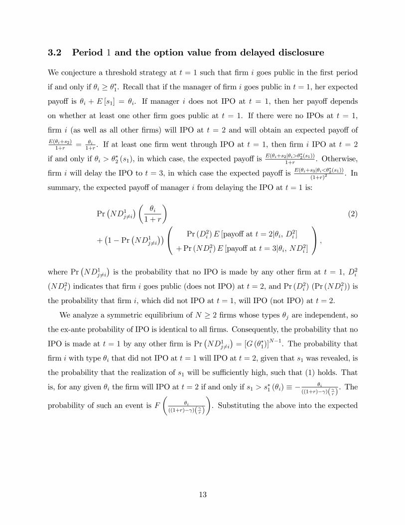
3.2 Period 1 and the option value from delayed disclosure

We conjecture a threshold strategy at t = 1 such that firm i goes public in the first period

if and only if θi ≥ θ∗1. Recall that if the manager of firm i goes public in t = 1, her expected

payoff is θi + E [s1] = θi. If manager i does not IPO at t = 1, then her payoff depends

on whether at least one other firm goes public at t = 1. If there were no IPOs at t = 1,

firm i (as well as all other firms) will IPO at t = 2 and will obtain an expected payoff ofE(θi+s2)1+r

= θi1+r. If at least one firm went through IPO at t = 1, then firm i IPO at t = 2

if and only if θi > θ∗2 (s1), in which case, the expected payoff isE(θi+s2|θi>θ∗2(s1))

1+r. Otherwise,

firm i will delay the IPO to t = 3, in which case the expected payoff is E(θi+s3|θi<θ∗2(s1))(1+r)2

. In

summary, the expected payoff of manager i from delaying the IPO at t = 1 is:

Pr(ND1

j 6=i)( θi

1 + r

)(2)

+(1− Pr

(ND1

j 6=i)) Pr (D2

i )E [payoff at t = 2|θi, D2i ]

+ Pr (ND2i )E [payoff at t = 3|θi, ND2

i ]

,

where Pr(ND1

j 6=i)is the probability that no IPO is made by any other firm at t = 1, D2

i

(ND2i ) indicates that firm i goes public (does not IPO) at t = 2, and Pr (D2

i ) (Pr (ND2i )) is

the probability that firm i, which did not IPO at t = 1, will IPO (not IPO) at t = 2.

We analyze a symmetric equilibrium of N ≥ 2 firms whose types θj are independent, so

the ex-ante probability of IPO is identical to all firms. Consequently, the probability that no

IPO is made at t = 1 by any other firm is Pr(ND1

j 6=i)

= [G (θ∗1)]N−1. The probability that

firm i with type θi that did not IPO at t = 1 will IPO at t = 2, given that s1 was revealed, is

the probability that the realization of s1 will be suffi ciently high, such that (1) holds. That

is, for any given θi the firm will IPO at t = 2 if and only if s1 > s∗1 (θi) ≡ − θi((1+r)−γ)( γr )

. The

probability of such an event is F(

θi((1+r)−γ)( γr )

). Substituting the above into the expected

13

payoff of the manager of firm i from not going public at t = 1, given in (2), yields:

[G (θ∗1)]N−1

(θ∗1

1 + r

)(3)

+(

1− [G (θ∗1)]N−1) F

(θi

((1+r)−γ)( γr )

)E [payoff at t = 2|θi, D2

i ]

+

(1− F

(θi

((1+r)−γ)( γr )

))E [payoff at t = 3|θi, ND2

i ]

.

Note that unlike the threshold in t = 2, which depends on the manager’s type and the

realization of s1, the IPO threshold of the first period, θ∗1, depends only on the firm’s type,

θi (and all the other parameters of the model).

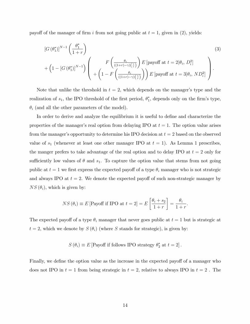
In order to derive and analyze the equilibrium it is useful to define and characterize the

properties of the manager’s real option from delaying IPO at t = 1. The option value arises

from the manager’s opportunity to determine his IPO decision at t = 2 based on the observed

value of s1 (whenever at least one other manager IPO at t = 1). As Lemma 1 prescribes,

the manger prefers to take advantage of the real option and to delay IPO at t = 2 only for

suffi ciently low values of θ and s1. To capture the option value that stems from not going

public at t = 1 we first express the expected payoff of a type θi manager who is not strategic

and always IPO at t = 2. We denote the expected payoff of such non-strategic manager by

NS (θi), which is given by:

NS (θi) ≡ E [Payoff if IPO at t = 2] = E

[θi + s21 + r

]=

θi1 + r

.

The expected payoff of a type θi manager that never goes public at t = 1 but is strategic at

t = 2, which we denote by S (θi) (where S stands for strategic), is given by:

S (θi) ≡ E [Payoff if follows IPO strategy θ∗2 at t = 2] .

Finally, we define the option value as the increase in the expected payoff of a manager who

does not IPO in t = 1 from being strategic in t = 2, relative to always IPO in t = 2 . The

14

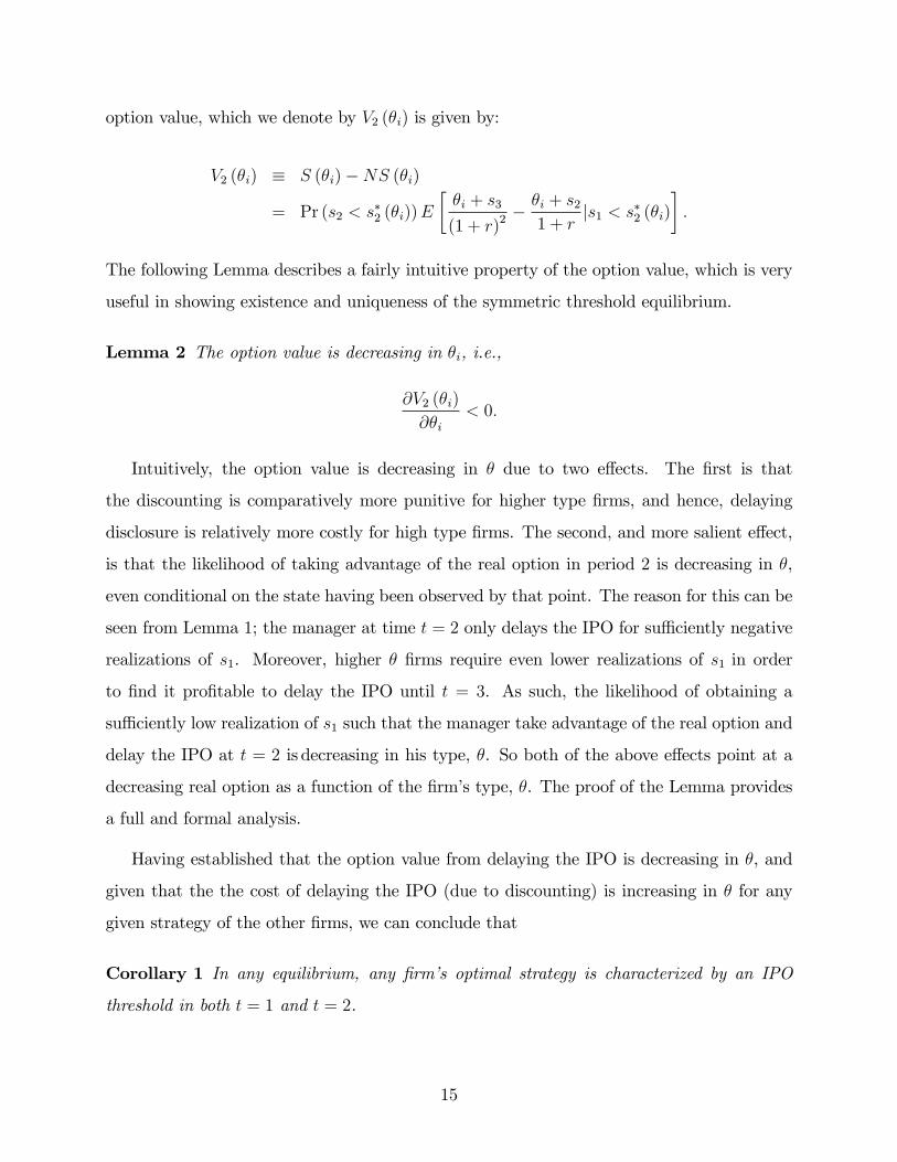
option value, which we denote by V2 (θi) is given by:

V2 (θi) ≡ S (θi)−NS (θi)

= Pr (s2 < s∗2 (θi))E

[θi + s3

(1 + r)2− θi + s2

1 + r|s1 < s∗2 (θi)

].

The following Lemma describes a fairly intuitive property of the option value, which is very

useful in showing existence and uniqueness of the symmetric threshold equilibrium.

Lemma 2 The option value is decreasing in θi, i.e.,

∂V2 (θi)

∂θi< 0.

Intuitively, the option value is decreasing in θ due to two effects. The first is that

the discounting is comparatively more punitive for higher type firms, and hence, delaying

disclosure is relatively more costly for high type firms. The second, and more salient effect,

is that the likelihood of taking advantage of the real option in period 2 is decreasing in θ,

even conditional on the state having been observed by that point. The reason for this can be

seen from Lemma 1; the manager at time t = 2 only delays the IPO for suffi ciently negative

realizations of s1. Moreover, higher θ firms require even lower realizations of s1 in order

to find it profitable to delay the IPO until t = 3. As such, the likelihood of obtaining a

suffi ciently low realization of s1 such that the manager take advantage of the real option and

delay the IPO at t = 2 is decreasing in his type, θ. So both of the above effects point at a

decreasing real option as a function of the firm’s type, θ. The proof of the Lemma provides

a full and formal analysis.

Having established that the option value from delaying the IPO is decreasing in θ, and

given that the the cost of delaying the IPO (due to discounting) is increasing in θ for any

given strategy of the other firms, we can conclude that

Corollary 1 In any equilibrium, any firm’s optimal strategy is characterized by an IPO

threshold in both t = 1 and t = 2.

15

We next solve for, and analyze, the symmetric equilibrium, in which all firms follow the

same strategy. We show that there is a unique symmetric equilibrium. While our main

focus is the symmetric equilibrium in the setting with an unbounded support, we study in

section 5 an extension of the model in which the support of firm’s type is bounded from

above, i.e., θ ∈[0, θ]. For this setting, the unique symmetric equilibrium still always exists,

however, for suffi ciently low discount factors we show the existence of another equilibrium,

in which one firm always goes public at t = 1 and all the other firms never IPO at t = 1.

Such an equilibrium does not exists in our main setting in which the support of firm’s type

is unbounded from above.

In a symmetric equilibrium, each manager’s best response to all other managers’strate-

gies, who play a threshold strategy θ∗1, is consequently given by θ∗1. The t = 1 the threshold

level of all firms is such that each manager of the threshold type, θ∗1, is indifferent between

going public and not going public at t = 1. Therefore, the threshold level is the type for

which θ∗1 equals the expected payoff from not going public at t = 1, given in equation (3).

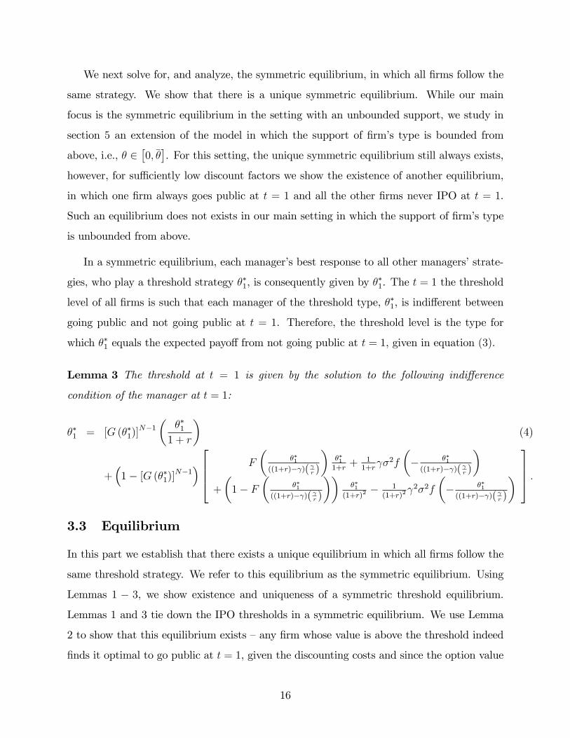
Lemma 3 The threshold at t = 1 is given by the solution to the following indifference

condition of the manager at t = 1:

θ∗1 = [G (θ∗1)]N−1

(θ∗1

1 + r

)(4)

+(

1− [G (θ∗1)]N−1) F

(θ∗1

((1+r)−γ)( γr )

)θ∗11+r

+ 11+r

γσ2f

(− θ∗1((1+r)−γ)( γr )

)+

(1− F

(θ∗1

((1+r)−γ)( γr )

))θ∗1

(1+r)2− 1

(1+r)2γ2σ2f

(− θ∗1((1+r)−γ)( γr )

) .

3.3 Equilibrium

In this part we establish that there exists a unique equilibrium in which all firms follow the

same threshold strategy. We refer to this equilibrium as the symmetric equilibrium. Using

Lemmas 1 − 3, we show existence and uniqueness of a symmetric threshold equilibrium.

Lemmas 1 and 3 tie down the IPO thresholds in a symmetric equilibrium. We use Lemma

2 to show that this equilibrium exists —any firm whose value is above the threshold indeed

finds it optimal to go public at t = 1, given the discounting costs and since the option value

16

is decreasing in θ. Moreover, we show that the threshold characterized by Lemma 1 and

Lemma 3 is the unique threshold level in the symmetric equilibrium.

Theorem 1 There exists a unique symmetric strategy in which firm i, i = 1, 2, ..N , uses the

following IPO threshold strategy:

(i) Firm i goes public at t = 1 if and only if θi ≥ θ∗1, where θ∗1 is given by the solution to (4);

(ii) if any other firm went public at t = 1 the firm i goes public at t = 2 if and only if

θi ≥ θ∗2 (s1) ≡ −s1 ((1 + r)− γ)(γr

)(when firm i did not IPO at t = 1);

(iii) if no IPO was made by any firm at t = 1 firm i goes at t = 2 for all θi.

Proof. Given that the IPO strategy of firm i at t = 2 does not depend on beliefs about θj,

the IPO strategy at t = 2 is given by (ii) and (iii) (note that if no other firm went public at

t = 1 we are back to a two-period setting, in which all firms IPO immediately as they can).

Under the assumption of existence of a threshold equilibrium, any IPO threshold at t = 1

should satisfy the first period’s indifference condition in (4).

At t = 2 the firm will IPO if an only if the expected payoff from IPO is higher than if it

delays the IPO, i.e., it will IPO if θi+E(s2|s1)1+r

≥ θi+E(s3|s1)(1+r)2

, which holds for all θi > θ∗2 (s1) =

−s1 ((1 + r)− γ)(γr

). Therefore, no type has an incentive to deviate at t = 2.

Next, we show that no type has an incentive to deviate at t = 1. Assume that type θi = θ∗1 is

indifferent between going public and delaying the IPO at t = 1. To show that all types higher

(lower) than θ∗1 strictly prefer to IPO (not to IPO) note that the marginal loss in delaying

the IPO for higher (lower) θi is greater (smaller) due to discounting, i.e. discounting is

more pronounced for higher θi’s. In addition, the marginal benefit from delaying the IPO

(captured by the option value) is lower (higher) for higher θi, as shown in Lemma 2. Hence,

no type has an incentive to deviate at t = 1.

Next, we show uniqueness of a symmetric IPO threshold. Assume by contradiction that

there are two values of θ∗1 : θL and θH where θH > θL, that are consistent with a symmetric

equilibrium. If all firms move from θL to θH , the probability that the other managers will

IPO decreases, which in turn increases any manager’s incentive to IPO. That is, it decreases

the best response IPO threshold. However, this contradicts the assumption of the existence

of a higher threshold θH . A similar argument follows for a lower IPO threshold. More

17

formally, the manager’s indifference condition at t = 1 is given by:

θi = Pr(ND1

j 6=i)( θi

1 + r

)

+(1− Pr

(ND1

j 6=i)) Pr (D2

i )E [payoff at t = 2|θi, and IPO at t = 2]

+ Pr (ND2i )E [payoff at t = 3|θi, and delay IPO at t = 2]

= Pr

(ND1

j 6=i)( θi

1 + r

)+(1− Pr

(ND1

j 6=i))(

Pr(D2i

) θi1 + r

+ Pr(ND2

i

)( θi1 + r

+ V2 (θi)

))=

θi1 + r

+(1− Pr

(ND1

j 6=i))

Pr(ND2

i

)V2 (θi) .

If the IPO threshold of firm j 6= i increases to θH , it has no effect on the option value

(conditional on getting to t = 2 when firm j went public at t = 1 and firm i’s type is

θi > θ∗2), however the probability of this event decreases as the threshold of firm i increases.

As such, the right hand side of the above indifference condition decreases, which implies

that, in order for firm i to be indifferent at t = 1, the IPO threshold of firm i at t = 1 must

decrease as well —in contradiction to the assumption of the increased IPO threshold.

Note that in obtaining the above results we imposed no restriction regarding the distribu-

tions of θ, and for tractability we assumed that εt is normally distributed (one can show that

the above Theorem holds for other distributions of the noise term, including distributions

with bounded support such as a uniform distribution).

In the next section we provide comparative statics and empirical predictions that come

out of the symmetric equilibrium.

4 Comparative Statics and Empirical Predictions

The first immediate prediction of the model is that firms with higher type, θ, go public earlier

than firms with lower type. Another immediate prediction is that following a “successful”

IPO in the first period, in which the state of nature turned out to be relatively high, we

expect clustering of IPOs. Our particular and stylized setting assumes that the distribution

of the innovation in the state of nature, ε, is symmetric, which implies that all firms will

IPO following a state of nature that is above the mean. However, under a more general

18

distribution of the innovation in the state of nature, higher realizations of the state of nature

in the first period increase the expected number of firms that will go public in the second

period. The following Corollary summarizes these immediate predictions of the model.

Corollary 2 In the unique symmetric equilibrium:

• The higher a firm’s type is the earlier it will disclose and go public.

• The expected number of IPOs in the second period, following an IPO in the first period

is increasing in the realization of the state of nature in the first period.

Next, we analyze how the equilibrium is affected by the various parameters. In particular,

we generate empirical predictions with respect to changes in the following parameters of the

model: the discount factor, the rate of mean reversion, and the variance of the error term.

We start by studying the effect of the parameters on the disclosure threshold in the second

period and then study the effect on the first period’s disclosure threshold.

4.1 Comparative Statics for θ∗2

We begin the analysis with the second period’s equilibrium threshold, θ∗2 (s1). Note that the

threshold of the second period, which is the unique best response at t = 2, is independent

of the other firm’s characteristics. So the analysis of this part is independent of whether the

firms are homogeneous or not and the specific characteristics of all the other firms.

Recall that the IPO threshold at t = 2, given that there was at least one IPO at t = 1

(and hence s1 is observed) is given by:

θ∗2 (s1) = −s1 ((1 + r)− γ)(γr

).

We will keep everything constant (including s1) and see how the threshold at t = 2 is affected

by changes in: (i) firm i’s manager discount factor, r; (ii) the extant of persistence in the

state of nature, γ (where lower γ implies higher mean-reversion); and (iii) the variance of

the shock to the state of nature , σε.

19

Taking the derivative of the threshold with respect to the discount factor, r, yields:

∂

∂rθ∗2 (s1) =

∂

∂r

(−s1 ((1 + r)− γ)

(γr

))= − 1

r2γs1 (γ − 1) < 0.

Note that ∂∂rθ∗2 (s1) < 0 since γ ∈ (0, 1) and at the threshold we have s1 < 0. The fact that

the threshold level at t = 2 is decreasing in r is very intuitive. To see that, recall that at the

IPO threshold θ∗2 (s1), at which the manager is indifferent between going public and delaying

the IPO, it must be that θ + s1 > 0 (otherwise the manager would strictly prefer to delay

the IPO to t = 3). Since the expected payoff of the threshold type is positive, an increase in

the discount factor increases the cost from delaying the IPO, and hence, decreases the IPO

threshold (equivalently, for a given θ the threshold level of s1 is lower).

Next we analyze the effect of the extant of mean-reversion of the state of nature, γ, on

the IPO threshold at t = 2. While the mathematical derivation of this effect is straight

forward, the intuition for the result is a little more complex.

Taking the derivative of the second period’s threshold with respect to γ, yields:

∂

∂γθ∗2 (s1) =

∂

∂γ

(−s1 ((1 + r)− γ)

(γr

))

= −1

rs1 (r − 2γ + 1) =

> 0 for γ < r+1

2

0 for γ = r+12

< 0 otherwise

.

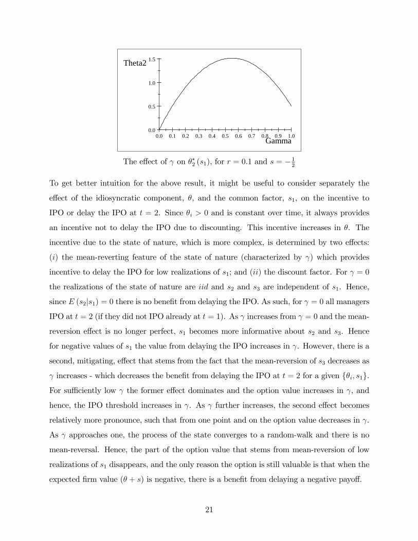
The direction of the effect of changes in γ on the threshold θ∗2 (s1) varies with the level of

γ. To illustrate the effect of γ on θ∗2 (s1), the figure below plots ∂∂γθ∗2 (s1) as a function of γ

using parameter values r = 0.1 and s = −12.

20

0.0 0.1 0.2 0.3 0.4 0.5 0.6 0.7 0.8 0.9 1.00.0

0.5

1.0

1.5

Gamma

Theta2

The effect of γ on θ∗2 (s1), for r = 0.1 and s = −12

To get better intuition for the above result, it might be useful to consider separately the

effect of the idiosyncratic component, θ, and the common factor, s1, on the incentive to

IPO or delay the IPO at t = 2. Since θi > 0 and is constant over time, it always provides

an incentive not to delay the IPO due to discounting. This incentive increases in θ. The

incentive due to the state of nature, which is more complex, is determined by two effects:

(i) the mean-reverting feature of the state of nature (characterized by γ) which provides

incentive to delay the IPO for low realizations of s1; and (ii) the discount factor. For γ = 0

the realizations of the state of nature are iid and s2 and s3 are independent of s1. Hence,

since E (s2|s1) = 0 there is no benefit from delaying the IPO. As such, for γ = 0 all managers

IPO at t = 2 (if they did not IPO already at t = 1). As γ increases from γ = 0 and the mean-

reversion effect is no longer perfect, s1 becomes more informative about s2 and s3. Hence

for negative values of s1 the value from delaying the IPO increases in γ. However, there is a

second, mitigating, effect that stems from the fact that the mean-reversion of s3 decreases as

γ increases - which decreases the benefit from delaying the IPO at t = 2 for a given θi, s1.

For suffi ciently low γ the former effect dominates and the option value increases in γ, and

hence, the IPO threshold increases in γ. As γ further increases, the second effect becomes

relatively more pronounce, such that from one point and on the option value decreases in γ.

As γ approaches one, the process of the state converges to a random-walk and there is no

mean-reversal. Hence, the part of the option value that stems from mean-reversion of low

realizations of s1 disappears, and the only reason the option is still valuable is that when the

expected firm value (θ + s) is negative, there is a benefit from delaying a negative payoff.

21

Finally, θ∗2 (s1) is independent of the variance in the noise of the state of nature, σ2, and

independent for the distribution of θ (recall that θ is assumed to have a positive support),

conditional on the state of nature s1 being revealed in t = 1. The threshold level in t = 2 is

consequently unaffected by changes in σ2.

4.2 Comparative Statics for θ∗1

The comparative statics for the first period threshold level, θ∗1, are slightly less intuitive,

however, the analysis of θ∗2 (s1) serves as a useful guide. We start with the effect of γ on θ∗1:

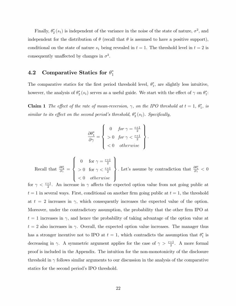
Claim 1 The effect of the rate of mean-reversion, γ, on the IPO threshold at t = 1, θ∗1, is

similar to its effect on the second period’s threshold, θ∗2 (s1). Specifically,

∂θ∗1∂γ

=

0 for γ = r+1

2

> 0 for γ < r+12

< 0 otherwise

.

Recall that ∂θ∗2∂γ

=

0 for γ = r+1

2

> 0 for γ < r+12

< 0 otherwise

. Let’s assume by contradiction that ∂θ∗1∂γ

< 0

for γ < r+12. An increase in γ affects the expected option value from not going public at

t = 1 in several ways. First, conditional on another firm going public at t = 1, the threshold

at t = 2 increases in γ, which consequently increases the expected value of the option.

Moreover, under the contradictory assumption, the probability that the other firm IPO at

t = 1 increases in γ, and hence the probability of taking advantage of the option value at

t = 2 also increases in γ. Overall, the expected option value increases. The manager thus

has a stronger incentive not to IPO at t = 1, which contradicts the assumption that θ∗1 is

decreasing in γ. A symmetric argument applies for the case of γ > r+12. A more formal

proof is included in the Appendix. The intuition for the non-monotonicity of the disclosure

threshold in γ follows similar arguments to our discussion in the analysis of the comparative

statics for the second period’s IPO threshold.

22

Next we analyze the effect of the discount factor, r, on the first period’s threshold. Similar

to the second period’s threshold, the first period threshold is also decreasing in the discount

rate:∂θ∗1∂r

< 0.

From the comparative statics for θ∗2, we know that∂θ∗2(s1)∂r

< 0, i.e., for a given level of θi the

manager is more likely to IPO in the second period for higher values of r, and hence, is less

likely to take advantage of the real option. In addition, a higher r increases the manager’s

cost from delaying the IPO. Both effects lead to a stronger incentive to IPO at t = 1. This

results in a lower IPO threshold at t = 1 for higher values of r.

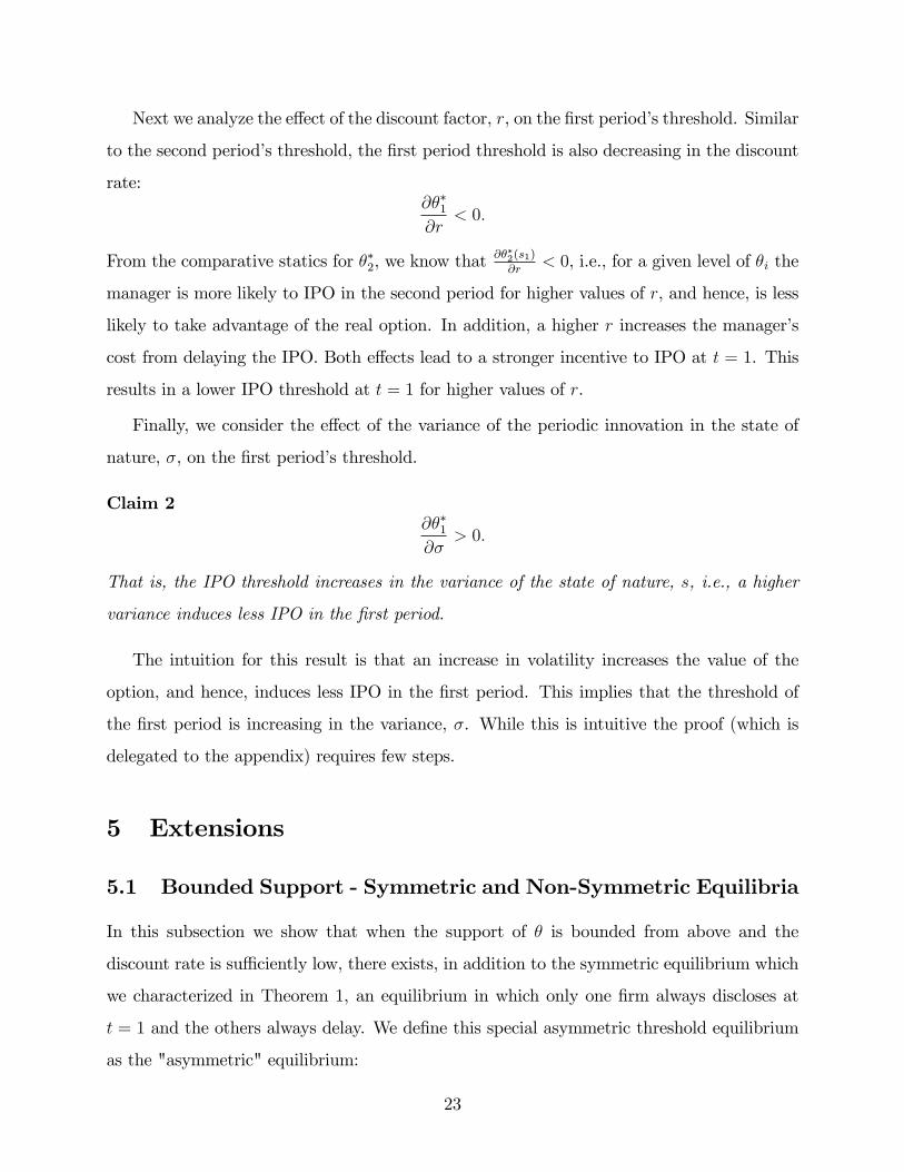
Finally, we consider the effect of the variance of the periodic innovation in the state of

nature, σ, on the first period’s threshold.

Claim 2∂θ∗1∂σ

> 0.

That is, the IPO threshold increases in the variance of the state of nature, s, i.e., a higher

variance induces less IPO in the first period.

The intuition for this result is that an increase in volatility increases the value of the

option, and hence, induces less IPO in the first period. This implies that the threshold of

the first period is increasing in the variance, σ. While this is intuitive the proof (which is

delegated to the appendix) requires few steps.

5 Extensions

5.1 Bounded Support - Symmetric and Non-Symmetric Equilibria

In this subsection we show that when the support of θ is bounded from above and the

discount rate is suffi ciently low, there exists, in addition to the symmetric equilibrium which

we characterized in Theorem 1, an equilibrium in which only one firm always discloses at

t = 1 and the others always delay. We define this special asymmetric threshold equilibrium

as the "asymmetric" equilibrium:

23

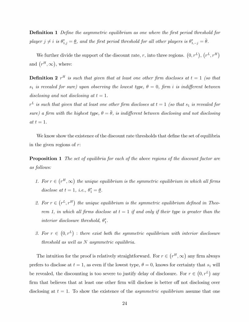
Definition 1 Define the asymmetric equilibrium as one where the first period threshold for

player j 6= i is θ∗1,j = θ, and the first period threshold for all other players is θ∗1,−j = θ.

We further divide the support of the discount rate, r, into three regions.(0, rL

),(rL, rH

)and

(rH ,∞

), where:

Definition 2 rH is such that given that at least one other firm discloses at t = 1 (so that

s1 is revealed for sure) upon observing the lowest type, θ = 0, firm i is indifferent between

disclosing and not disclosing at t = 1.

rL is such that given that at least one other firm discloses at t = 1 (so that s1 is revealed for

sure) a firm with the highest type, θ = θ, is indifferent between disclosing and not disclosing

at t = 1.

We know show the existence of the discount rate thresholds that define the set of equilibria

in the given regions of r:

Proposition 1 The set of equilibria for each of the above regions of the discount factor are

as follows:

1. For r ∈(rH ,∞

)the unique equilibrium is the symmetric equilibrium in which all firms

disclose at t = 1, i.e., θ∗1 = θ.

2. For r ∈(rL, rH

)the unique equilibrium is the symmetric equilibrium defined in Theo-

rem 1, in which all firms disclose at t = 1 if and only if their type is greater than the

interior disclosure threshold, θ∗1.

3. For r ∈(0, rL

): there exist both the symmetric equilibrium with interior disclosure

threshold as well as N asymmetric equilibria.

The intuition for the proof is relatively straightforward. For r ∈(rH ,∞

)any firm always

prefers to disclose at t = 1, as even if the lowest type, θ = 0, knows for certainty that s1 will

be revealed, the discounting is too severe to justify delay of disclosure. For r ∈(0, rL

)any

firm that believes that at least one other firm will disclose is better off not disclosing over

disclosing at t = 1. To show the existence of the asymmetric equilibrium assume that one

24

firm, firm i, always discloses at t = 1. The best response of all other firms is not to disclose

at t = 1. Now, given that the probability that any other firm will disclose at t = 1 is zero,

it is optimal for firm i to disclose at t = 1. So for r ∈(0, rL

)there exist N asymmetric

equilibria such that in each one of them a single firm always discloses at t = 1 and all the

other firms do not disclose at t = 1. Finally, for r ∈(rL, rH

)there are suffi ciently high types

that will disclose at t = 1 even if they are certain that s1 will be observed. Hence, there is

always a positive probability that at least one firm will disclose at t = 1. Let’s assume by

contradiction that there exists an asymmetric equilibrium in which firm i always discloses.

Then, there exists a disclosure threshold, such that any other firm discloses if and only if its

type is lower than this threshold. This, however implies that there is a positive probability

that a firm other than firm i will disclose at t = 1. As such, if the realized type of firm i is

suffi ciently low, the discount effect can be arbitrarily low and the value of the real option is

strictly positive. Therefore, firm i will disclose for suffi ciently low types - in contradiction to

the assumption that firm i does not disclose.

6 Conclusion

In this study we have developed a model to help shed light on the strategic interaction

between firms who decide to disclose information and sell shares or a project. We have

shown that the unique equilibrium is in threshold strategies where all players follow identical

strategies. The primary implication of this result is that, in the presence of other firms and

common uncertainty, there is always a positive amount of delay of IPOs in equilibrium.

Several extensions can be considered for future work. We have considered only cases

in which the disclosure of the firm’s value if verifiable and non-manipulable. A possibly

interesting study would be to relax this assumption, in which case firm managers can engage

in costly manipulation of the firm’s value. We have also assumed that the firm’s type

(idiosyncratic component) is constant over time. A potentially interesting research question

is to investigate a model where the firm’s value also follows a stochastic process. Lastly,

our model can be extended to a continuous time setting with finite number of firms. We

conjecture that in a continuous time setting there exists an equilibrium in which each firm’s

25

delay of the IPO is decreasing in the firm’s type and the more negative the revealed state

of nature is, the more firms delay their IPOs. As such, the continuous time setting seem to

share the main characteristics of our discrete time model.

26

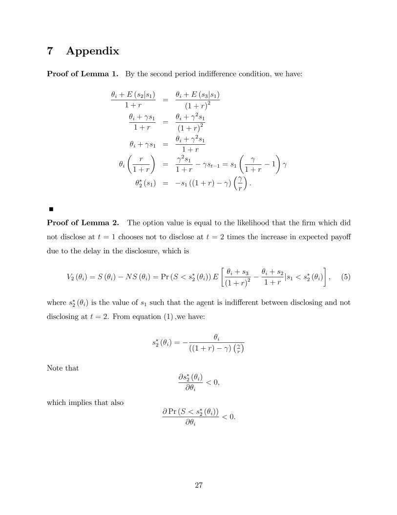
7 Appendix

Proof of Lemma 1. By the second period indifference condition, we have:

θi + E (s2|s1)1 + r

=θi + E (s3|s1)

(1 + r)2

θi + γs11 + r

=θi + γ2s1

(1 + r)2

θi + γs1 =θi + γ2s1

1 + r

θi

(r

1 + r

)=

γ2s11 + r

− γst−1 = s1

(γ

1 + r− 1

)γ

θ∗2 (s1) = −s1 ((1 + r)− γ)(γr

).

Proof of Lemma 2. The option value is equal to the likelihood that the firm which did

not disclose at t = 1 chooses not to disclose at t = 2 times the increase in expected payoff

due to the delay in the disclosure, which is

V2 (θi) = S (θi)−NS (θi) = Pr (S < s∗2 (θi))E

[θi + s3

(1 + r)2− θi + s2

1 + r|s1 < s∗2 (θi)

], (5)

where s∗2 (θi) is the value of s1 such that the agent is indifferent between disclosing and not

disclosing at t = 2. From equation (1) ,we have:

s∗2 (θi) = − θi

((1 + r)− γ)(γr

)Note that

∂s∗2 (θi)

∂θi< 0,

which implies that also∂ Pr (S < s∗2 (θi))

∂θi< 0.

27

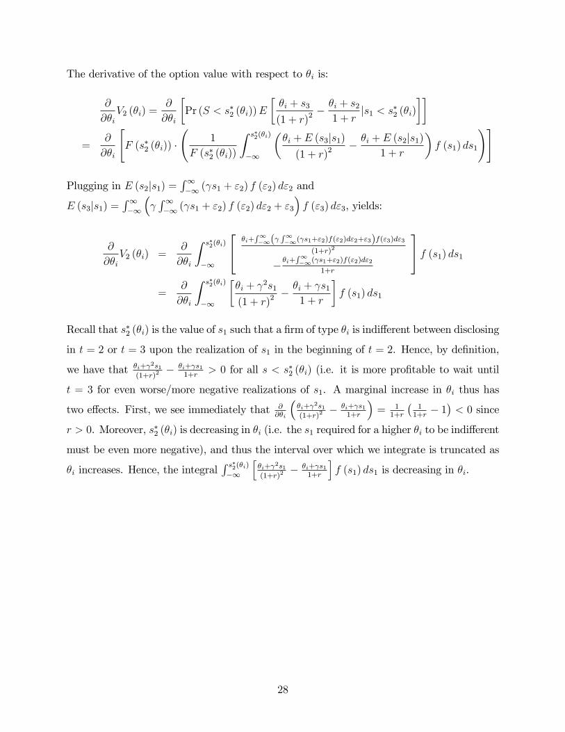
The derivative of the option value with respect to θi is:

∂

∂θiV2 (θi) =

∂

∂θi

[Pr (S < s∗2 (θi))E

[θi + s3

(1 + r)2− θi + s2

1 + r|s1 < s∗2 (θi)

]]=

∂

∂θi

[F (s∗2 (θi)) ·

(1

F (s∗2 (θi))

∫ s∗2(θi)

−∞

(θi + E (s3|s1)

(1 + r)2− θi + E (s2|s1)

1 + r

)f (s1) ds1

)]

Plugging in E (s2|s1) =∫∞−∞ (γs1 + ε2) f (ε2) dε2 and

E (s3|s1) =∫∞−∞

(γ∫∞−∞ (γs1 + ε2) f (ε2) dε2 + ε3

)f (ε3) dε3, yields:

∂

∂θiV2 (θi) =

∂

∂θi

∫ s∗2(θi)

−∞

θi+∫∞−∞(γ

∫∞−∞(γs1+ε2)f(ε2)dε2+ε3)f(ε3)dε3

(1+r)2

− θi+∫∞−∞(γs1+ε2)f(ε2)dε2

1+r

f (s1) ds1

=∂

∂θi

∫ s∗2(θi)

−∞

[θi + γ2s1

(1 + r)2− θi + γs1

1 + r

]f (s1) ds1

Recall that s∗2 (θi) is the value of s1 such that a firm of type θi is indifferent between disclosing

in t = 2 or t = 3 upon the realization of s1 in the beginning of t = 2. Hence, by definition,

we have that θi+γ2s1

(1+r)2− θi+γs1

1+r> 0 for all s < s∗2 (θi) (i.e. it is more profitable to wait until

t = 3 for even worse/more negative realizations of s1. A marginal increase in θi thus has

two effects. First, we see immediately that ∂∂θi

(θi+γ

2s1(1+r)2

− θi+γs11+r

)= 1

1+r

(11+r− 1)< 0 since

r > 0. Moreover, s∗2 (θi) is decreasing in θi (i.e. the s1 required for a higher θi to be indifferent

must be even more negative), and thus the interval over which we integrate is truncated as

θi increases. Hence, the integral∫ s∗2(θi)−∞

[θi+γ

2s1(1+r)2

− θi+γs11+r

]f (s1) ds1 is decreasing in θi.

28

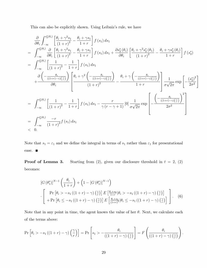
This can also be explicitly shown. Using Leibniz’s rule, we have

∂

∂θi

∫ s∗2(θi)

−∞

[θi + γ2s1

(1 + r)2− θi + γs1

1 + r

]f (s1) ds1

=

∫ s∗2(θi)

−∞

∂

∂θi

[θi + γ2s1

(1 + r)2− θi + γs1

1 + r

]f (s1) ds1 +

∂s∗2 (θi)

∂θi

[θi + γ2s∗2 (θ1)

(1 + r)2− θi + γs∗2 (θi)

1 + r

]f (s∗2)

=

∫ s∗2(θi)

−∞

[1

(1 + r)2− 1

1 + r

]f (s1) ds1

+

∂

(− θi((1+r)−γ)( γr )

)∂θi

θi + γ2(− θi((1+r)−γ)( γr )

)(1 + r)2

−θi + γ

(− θi((1+r)−γ)( γr )

)1 + r

1

σ√

2πexp

[−(s∗2)

2

2σ2

]

=

∫ s∗2(θi)

−∞

[1

(1 + r)2− 1

1 + r

]f (s1) ds1 −

r

γ (r − γ + 1)[0]

1

σ√

2πexp

−(− θi((1+r)−γ)( γr )

)22σ2

=

∫ s∗2(θi)

−∞

−r(1 + r)2

f (s1) ds1

< 0.

Note that s1 = ε1 and we define the integral in terms of s1 rather than ε1 for presentational

ease.

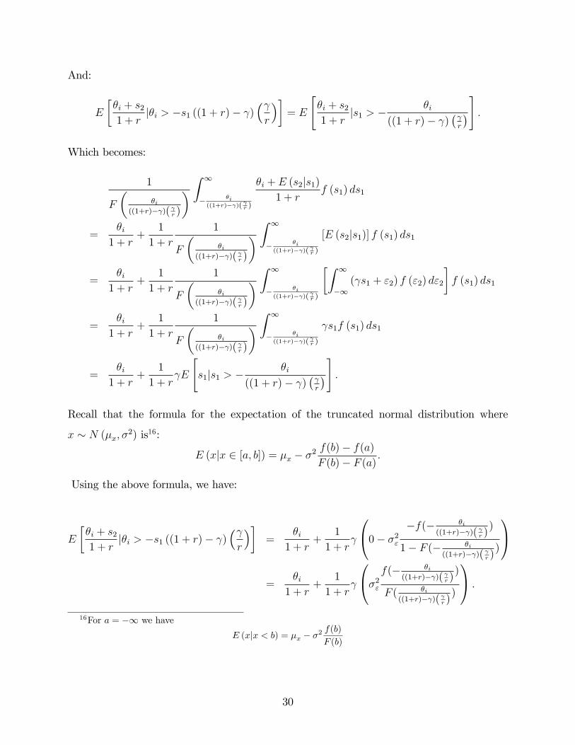
Proof of Lemma 3. Starting from (2), given our disclosure threshold in t = 2, (2)

becomes:

[G (θ∗1)]N−1

(θi

1 + r

)+(

1− [G (θ∗1)]N−1)

·

Pr[θi > −s1 ((1 + r)− γ)

(γr

)]E[θi+s21+r|θi > −s1 ((1 + r)− γ)

(γr

)]+ Pr

[θi ≤ −s1 ((1 + r)− γ)

(γr

)]E[θi+s3(1+r)2

|θi ≤ −s1 ((1 + r)− γ)(γr

)] . (6)

Note that in any point in time, the agent knows the value of her θ. Next, we calculate each

of the terms above:

Pr[θi > −s1 ((1 + r)− γ)

(γr

)]= Pr

[s1 > −

θi

((1 + r)− γ)(γr

)] = F

(θi

((1 + r)− γ)(γr

)) .

29

And:

E

[θi + s21 + r

|θi > −s1 ((1 + r)− γ)(γr

)]= E

[θi + s21 + r

|s1 > −θi

((1 + r)− γ)(γr

)] .Which becomes:

1

F

(θi

((1+r)−γ)( γr )

) ∫ ∞− θi((1+r)−γ)( γr )

θi + E (s2|s1)1 + r

f (s1) ds1

=θi

1 + r+

1

1 + r

1

F

(θi

((1+r)−γ)( γr )

) ∫ ∞− θi((1+r)−γ)( γr )

[E (s2|s1)] f (s1) ds1

=θi

1 + r+

1

1 + r

1

F

(θi

((1+r)−γ)( γr )

) ∫ ∞− θi((1+r)−γ)( γr )

[∫ ∞−∞

(γs1 + ε2) f (ε2) dε2

]f (s1) ds1

=θi

1 + r+

1

1 + r

1

F

(θi

((1+r)−γ)( γr )

) ∫ ∞− θi((1+r)−γ)( γr )

γs1f (s1) ds1

=θi

1 + r+

1

1 + rγE

[s1|s1 > −

θi

((1 + r)− γ)(γr

)] .Recall that the formula for the expectation of the truncated normal distribution where

x ∼ N (µx, σ2) is16:

E (x|x ∈ [a, b]) = µx − σ2f(b)− f(a)

F (b)− F (a).

Using the above formula, we have:

E

[θi + s21 + r

|θi > −s1 ((1 + r)− γ)(γr

)]=

θi1 + r

+1

1 + rγ

0− σ2ε−f(− θi

((1+r)−γ)( γr ))

1− F (− θi((1+r)−γ)( γr )

)

=

θi1 + r

+1

1 + rγ

σ2ε f(− θi((1+r)−γ)( γr )

)

F ( θi((1+r)−γ)( γr )

)

.

16For a = −∞ we have

E (x|x < b) = µx − σ2f(b)

F (b)

30

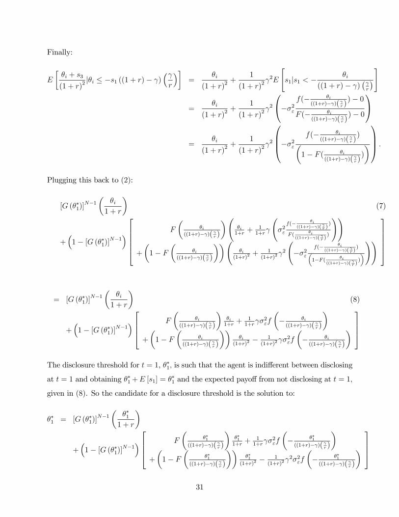
Finally:

E

[θi + s3

(1 + r)2|θi ≤ −s1 ((1 + r)− γ)

(γr

)]=

θi

(1 + r)2+

1

(1 + r)2γ2E

[s1|s1 < −

θi

((1 + r)− γ)(γr

)]

=θi

(1 + r)2+

1

(1 + r)2γ2

−σ2ε f(− θi((1+r)−γ)( γr )

)− 0

F (− θi((1+r)−γ)( γr )

)− 0

=θi

(1 + r)2+

1

(1 + r)2γ2

−σ2ε f(− θi((1+r)−γ)( γr )

)(1− F ( θi

((1+r)−γ)( γr ))

) .

Plugging this back to (2):

[G (θ∗1)]N−1

(θi

1 + r

)(7)

+(

1− [G (θ∗1)]N−1)

F

(θi

((1+r)−γ)( γr )

)(θi1+r

+ 11+r

γ

(σ2ε

f(− θi((1+r)−γ)( γr )

)

F (θi

((1+r)−γ)( γr ))

))

+

(1− F

(θi

((1+r)−γ)( γr )

))(θi

(1+r)2+ 1

(1+r)2γ2

(−σ2ε

f(− θi((1+r)−γ)( γr )

)(1−F ( θi

((1+r)−γ)( γr ))

)))

= [G (θ∗1)]N−1

(θi

1 + r

)(8)

+(

1− [G (θ∗1)]N−1) F

(θi

((1+r)−γ)( γr )

)θi1+r

+ 11+r

γσ2εf

(− θi((1+r)−γ)( γr )

)+

(1− F

(θi

((1+r)−γ)( γr )

))θi

(1+r)2− 1

(1+r)2γσ2εf

(− θi((1+r)−γ)( γr )

)

The disclosure threshold for t = 1, θ∗1, is such that the agent is indifferent between disclosing

at t = 1 and obtaining θ∗1 +E [s1] = θ∗1 and the expected payoff from not disclosing at t = 1,

given in (8). So the candidate for a disclosure threshold is the solution to:

θ∗1 = [G (θ∗1)]N−1

(θ∗1

1 + r

)

+(

1− [G (θ∗1)]N−1) F

(θ∗1

((1+r)−γ)( γr )

)θ∗11+r

+ 11+r

γσ2εf

(− θ∗1((1+r)−γ)( γr )

)+

(1− F

(θ∗1

((1+r)−γ)( γr )

))θ∗1

(1+r)2− 1

(1+r)2γ2σ2εf

(− θ∗1((1+r)−γ)( γr )

)

31

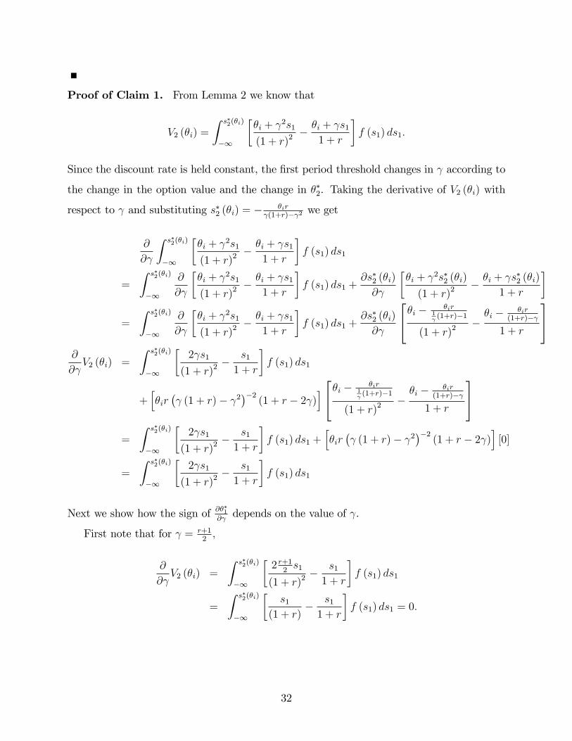
Proof of Claim 1. From Lemma 2 we know that

V2 (θi) =

∫ s∗2(θi)

−∞

[θi + γ2s1

(1 + r)2− θi + γs1

1 + r

]f (s1) ds1.

Since the discount rate is held constant, the first period threshold changes in γ according to

the change in the option value and the change in θ∗2. Taking the derivative of V2 (θi) with

respect to γ and substituting s∗2 (θi) = − θirγ(1+r)−γ2 we get

∂

∂γ

∫ s∗2(θi)

−∞

[θi + γ2s1

(1 + r)2− θi + γs1

1 + r

]f (s1) ds1

=

∫ s∗2(θi)

−∞

∂

∂γ

[θi + γ2s1

(1 + r)2− θi + γs1

1 + r

]f (s1) ds1 +

∂s∗2 (θi)

∂γ

[θi + γ2s∗2 (θi)

(1 + r)2− θi + γs∗2 (θi)

1 + r

]

=

∫ s∗2(θi)

−∞

∂

∂γ

[θi + γ2s1

(1 + r)2− θi + γs1

1 + r

]f (s1) ds1 +

∂s∗2 (θi)

∂γ

θi − θir1γ(1+r)−1

(1 + r)2−θi − θir

(1+r)−γ

1 + r

∂

∂γV2 (θi) =

∫ s∗2(θi)

−∞

[2γs1

(1 + r)2− s1

1 + r

]f (s1) ds1

+[θir(γ (1 + r)− γ2

)−2(1 + r − 2γ)

]θi − θir1γ(1+r)−1

(1 + r)2−θi − θir

(1+r)−γ

1 + r

=

∫ s∗2(θi)

−∞

[2γs1

(1 + r)2− s1

1 + r

]f (s1) ds1 +

[θir(γ (1 + r)− γ2

)−2(1 + r − 2γ)

][0]

=

∫ s∗2(θi)

−∞

[2γs1

(1 + r)2− s1

1 + r

]f (s1) ds1

Next we show how the sign of ∂θ∗1

∂γdepends on the value of γ.

First note that for γ = r+12,

∂

∂γV2 (θi) =

∫ s∗2(θi)

−∞

[2 r+1

2s1

(1 + r)2− s1

1 + r

]f (s1) ds1

=

∫ s∗2(θi)

−∞

[s1

(1 + r)− s1

1 + r

]f (s1) ds1 = 0.

32

For γ > r+12, we have that:

∫ s∗2(θi)

−∞

[2γs1

(1 + r)2− s1

(1 + r)

]f (s1) ds1 < 0.

And finally, for γ < r+12:

∫ s∗2(θi)

−∞

[2γs1

(1 + r)2− s1

(1 + r)

]f (s1) ds1 > 0.

Since θ∗2 follows the same direction as the change in the option value, the behavior of θ∗1 can

be characterized by the above. For example, for γ < r+12, since ∂θ∗2

∂γ> 0 and ∂

∂γV2 (θi) > 0,

then ∂θ∗1∂γ. I.e. since the option value increases in γ < r+1

2, the period 1 threshold will

increase since it waiting becomes more valuable, while the cost of waiting, r, remains the

same. Likewise, since the second period threshold increases in γ < r+12, the likelihood of

taking advantage of the real option is increasing for fixed s1, thus making the real option

more valuable, resulting in an increased period one threshold for fixed r. Both of these effects

work in the same direction and hence the θ∗1 is increasing in γ <r+12. A similar argument

applies for γ > r+12and γ = r+1

2.

Proof of Claim 2. Recall that the disclosure threshold in the second period, θ∗2 (s1), is

independent of σ. In addition, for any θ the manager will disclose for any s1 > µs = 0. So,

the manager will take advantage of the real option only for suffi ciently low realizations of s1,

which are all lower than the mean of s1.

An increase in σ, increases the probability that a manager that does not disclose at t = 1

will take advantage of the real option (and delay disclosure to t = 3). This however, is not

suffi cient to increase the incentive to delay disclosure at t = 1. A suffi cient argument for the

comparative static is to keep the threshold at t = 1 constant and to show that following an

increase in σ the manager is no longer indifferent between disclosing and not disclosing for

θ = θ∗1 but rather strictly prefers not to disclose at t = 1.

A type θ∗1 will disclose at t = 2 either if the other manager did not disclose at t = 1 or

if s1 is lower than a threshold s∗2 (θi) = − θi((1+r)−γ)( γr )

. So the value from delaying disclosure

comes only from realizations s1 < s∗2 (θi) < 0. First, note that following an increase in σ

33

the probability of a realization of s1 < s∗2 (θi) increases, i.e.,∂ Pr(s1<s∗2(θi))

∂σ> 0. Second, the

expected value from delaying disclosure decreases in s1.

There exists a value s′ such that for all s1 < s′ the probability of such an s1 increases

in σ. If s′ > s∗2 (θi) that completes the proof. For s′ < s∗2 (θi), following an increase in σ

the probability of s1 < s′ increase where Pr (s1 ∈ (s′, s∗2 (θi))) decreases. It can be shown

that we can “shift”mass from realization s1 < s′ to realization (s1 ∈ (s′, s∗2 (θi))) under the

high variance distribution such that pdf for all (s1 ∈ (s′, s∗2 (θi))) will be identical to the

distribution with the low variance. Note that any such shift decreases the expected value

from delaying disclosure at t = 1. Since the cumulative distribution for s1 < s∗2 (θi) is higher

under the high variance distribution, following this “shifting procedure”for any s1 < s′ the

pdf under the new distribution is still higher than under the low variance distribution (since

the overall mass for s1 < s∗2 (θi) is higher for the high variance distribution). This implies

that the option value under the high variance distribution is strictly higher than under the

low variance distribution.

Proof of Proposition 1. Assume that in the case of indifference, the firm discloses. Note

that when r = 0, we have no interior solution. The only equilibria are asymmetric equilibria.

It is easy to show that these are equilibria and that no interior equilibrium exists—in any

equilibrium in which firm j discloses with positive probability, type θi is better off waiting

with probability 1, as this gives her strictly higher expected utility over disclosing when

r = 0. Note that there always exists an r > 0 in which we have the asymmetric equilibria.

34

Setting G(θ∗1,j)

= 0, we have from Lemma 3 that, as r → 0,

limr→0

G(θ∗j)( θ∗i

1 + r

)

+(1−G

(θ∗j)) F

(θ∗i

((1+r)−γ)( γr )

)θ∗11+r

+ 11+r

γσ2f

(− θ∗i((1+r)−γ)( γr )

)+

(1− F

(θ∗i

((1+r)−γ)( γr )

))θ∗1

(1+r)2− 1

(1+r)2γ2σ2f

(− θ∗i((1+r)−γ)( γr )

)

= F (0)θ∗i

1 + r+

1

1 + rγσ2f

(− rγ· θ∗i

((1 + r)− γ)

)+ (1− F (0))

θ∗i(1 + r)2

− 1

(1 + r)2γ2σ2f

(− rγ· θ∗i

((1 + r)− γ)

).

= F (0) θ∗i + γσ2f (0) + (1− F (0)) θ∗i − γ2σ2f (0)

= θ∗i + γσ2f (0)− γ2σ2f (0)

= θ∗i + σ2f (0)(γ − γ2

)= θ∗i + σ2

1

σ√

2πe−

µ

2σ2 γ (1− γ)

= θ∗i +σ

e√

2πγ (1− γ) .

Since γ ∈ (0, 1) and σ > 0, the benefit of waiting in the limit is strictly positive. Hence, for

all σ > 0 and γ ∈ (0, 1), we can find r suffi ciently close to zero such that an asymmetric

equilibrium can be supported when G(θ∗1,j)

= 0. Recall that the upper bound of the

asymmetric equilibria is denoted by rL. Now for any r > rL, type θ−j still finds disclosure

profitable even when G(θ∗1,j)

= 0, and hence the asymmetric equilibria do not exist for

r > rL. Finally, as r → ∞, the payoff from waiting to disclose goes to zero. For θ with

bounded support, we can find an r < ∞ such that θ∗i ≤ θ when G(θ∗j)

= 0. Denote the

maximum r that supports this equilibrium as rH :

rH = maxr

Pr(s1 >

rγ· −θi((1+r)−γ)

)E[θi+s21+r|s1 > r

γ· −θi((1+r)−γ)

]+(

Pr(s1 <

rγ· −θi((1+r)−γ)

))E[θi+s3(1+r)2

|s1 ≤ rγ· −θi((1+r)−γ)

]< θ

.Which we know exists by Theorem 1.

35

References

[1] Acharya, Viral V., Peter DeMarzo, and Ilan Kremer. 2011. “Endogenous Information

Flows and the Clustering of Announcements.” American Economic Review 101 (7):

2955—79.

[2] Alti, Aydogan. 2005. "IPO Market Timing." Review of Financial Studies 18 (3): 1105-

1138.

[3] Benninga, Simon, Mark Helmantel, and Oded Sarig. 2005. "The Timing of Initial Public

Offerings." Journal of Financial Economics 75: 115-32.

[4] Bessembinder, Hendrik, Jay F. Coughenour, Paul J. Seguin, and Margaret Monroe

Smoller. 1995. "Mean Reversion in Equilibrium Asset Prices: Evidence From the Futures

Term Structure." Journal of Finance 5 (1): 361-375.

[5] Bloom, Nicholas. 2009. "The Impact of Uncertainty Shocks." Econometrica 77 (3): 623-

685.

[6] Bloom, Nicholas, Max Floetotto, Nir Jaimovich, Itay Saporta, and Stephen Terry. 2014.

"Really Uncertain Business Cycles." Working paper.

[7] Cecchetti, Stephen G., Pok-Sang Lam, and Nelson C. MarkSource. "Mean Reversion in

Equilibrium Asset Prices." American Economic Review 80 (3): 398-418.

[8] Chemmanur, Thomas J., and Paolo Fulghieri. 1999. "A Theory of the Going-Public

Decision." Review of Financial Studies 12 (2): 249-79.

[9] Dembosky, April. "Wall Street ’mispriced’LinkedIn’s IPO." Financial Times, March

30, 2011.

[10] Demos, Telis, and Bradley Hope. "For Virtu IPO, Book Prompts A Delay." The Wall

Street Journal, April 3, 2014.

[11] Driebusch, Corrie, and Daniel Huang. "Bank IPO Falls Short of Targeted Price Range."

The Wall Street Journal, September 14, 2014.

36

[12] Dye, Ronald A. 1985. “Disclosure of Nonproprietary Information.”Journal of Account-

ing Research 23 (1): 123—45.

[13] Dye, Ronald A., and Sri S. Sridhar. 1995. “Industry-Wide Disclosure Dynamics.”Jour-

nal of Accounting Research 33(1): 157—74.

[14] Fama, Eugene F., and Kenneth R. French. 1988. "Permanent and Temporary Compo-

nents of Stock Prices." Journal of Political Economy 96 (2): 246-73.

[15] Guttman, Ilan, Ilan Kremer, and Andrzej Skrzypacz. 2014. "Not Only What but Also

When: A Theory of Dynamic Voluntary Disclosure." American Economic Review 104

(8): 2400—2420

[16] He, Ping. 2007. "A Theory of IPOWaves."Review of Financial Studies 20 (4): 983-1020.

[17] Helwege, Jean, and Nellie Liang. 2004. "Initial Public Offerings in Hot and Cold Mar-

kets." Journal of Financial and Quantitative Analysis 39 (3): 541-69.

[18] Jung, Woon-Oh, and Young K. Kwon. 1988. “Disclosure When the Market Is Unsure of

Information Endowment of Managers.”Journal of Accounting Research 26 (1): 146—53.

[19] Lerner, Joshua. 1994. "Venture capitalists and the decision to go public." Journal of

Financial Economics 35: 293-316.

[20] Loughran, Tim, Jay R. Ritter, and Kristen Rydqvist. 1994. "Initial public offerings:

International insights." Pacific-Basin Finance Journal 2: 166-99.

[21] Pagano, Marco, Fabio Panetta, and Luigi Zingales. 1998. "Why Do Companies Go

Public? An Empirical Analysis." Journal of Finance 53 (1): 27-64.

[22] Pastor, Lubos, and Pietro Veronesi. 2005. "Rational IPO Waves." Journal of Finance

60 (4): 1713-57.

[23] Persons, John C., and Vincent A. Warther. 1997. "Boom and Bust Patterns in the

Adoption of Financial Innovations." Review of Financial Studies 10 (4): 939-967.

37

[24] Poterba, James M., and Lawrence H. Summers. 1988. "Mean Reversion in Stock Prices."

Journal of Financial Economics 22: 27-59.

[25] Richards, Anthony J. 1997. "Winner-Loser Reversals in National Stock Market Idices:

Can they be explained?" Journal of Finance 52: 2129-44.

[26] Tobak, Steve. "Did IPO damage Facebook brand?" CBS Money Watch, June 6, 2012.

[27] Winkler, Rolfe, Matt Jarzemsky, and Evelyn Rusli. "Drop in Tech Stocks Hits Startup

Funding." The Wall Street Journal, April 16, 2014.

38