MASTER THESIS INCOMPUTER SCIENCEWith Emphasis in Intelligent Logistics ManagementThesis no: MSC-2007: 09March 2007

Strategies for Improving the Performance of Intermodal Line Train Cargo Systems

Author:

Muh Patrick Tatambunkah

Department of Systems and Software Engineering Blekinge Institute of TechnologyBox 520SE – 372 25 RonnebySweden

This thesis is submitted to the Department of systems and Software Engineering at the Blekinge Institute of Technology in partial fulfillment of the requirements for the degree of Master of Science in computer science with Emphasis in Intelligent Logistics Management. The thesis is equivalent to 20 weeks of full time studies.

Contact InformationAuthor: Muh Patrick TatambunkahE-mail: muhpat@yahoo.com

University Advisor:Dr. Jan A Persson.

Department of system and software EngineeringSchool of Engineering Blekinge Institute of technologyBox 214SE – 374 24 KarlshamnSweden

Internet: www.ipd.bth.se/jps/Phone: +46 454 38 59 06 (Karlshamn) Fax: + 46 454 191 04 (Karlshamn)E-mail: jan.persson@bth.se

- 3 -

PASSENGER TRAIN FREIGHT TRAIN

Abstract

With increasing trade, freight transport demand has grown tremendously and as sustainability has become an essential concern of our globe, interests in improving and achieving effective and efficient rail freight transport have become an essential needs and focus of the 21st century. However, achieving an improved rail freight transport service and an increased market share in a competitive environment is rather complex in several aspects as freight trains would need to operate with principles and characteristics resembling those of passenger’s traffic in order to attract new type of goods.

In order to adopt the principles and characteristics used in passenger trains, airlines and hotel industries into intermodal line train systems, a simulation model has been developed and implemented. The principles for pricing which we have considered are base on the available train capacity along a travel sub-leg and our objective was to increase the performance of the intermodal line cargo train system. We adopted the yield management concept with rail freight customers given the possibility to change their start and/or end train stations (travel sub-leg) and/or to change their departure day in an intermodal line cargo train system. Using our developed simulation tool, we have examined the performance of an intermodal line cargo train system with respect to the dynamic and constant pricing strategy. Our prime objective was to investigate and answer the questions which pricing strategy leads to the best space utilization and performance of an intermodal line train cargo system? Our simulation results show that the dynamic pricing gives the best space utilization and rail freight performance. Dynamic pricing strategy appears good to both the train operators, in term of the revenue generated, and the freight transporters as they achieved reduced transport cost and freights accommodation at train stations different from their closest train stations.

Keywords: strategy, performance improvement, combined rail-truck transport

- 4 -

Table of Contents

Abstract ........................................................................................................................................ 31 Introduction .......................................................................................................................... 6

1.1 Background ........................................................................................................................ 61.2 Purpose............................................................................................................................. 81.3 Research Questions ............................................................................................................ 91.4 Research Methodology....................................................................................................... 91.5 Literature Review............................................................................................................. 111.6 Why Combined Rail-Truck Freight transport .................................................................. 131.7 Limitations ....................................................................................................................... 141.8 Outline of the thesis ......................................................................................................... 15

2 Problem Description and modeling.................................................................................. 162.3 Transport services offered by the train and truck............................................................. 18

2.4.1 Constant Pricing Strategy.......................................................................................... 192.4.2 Dynamic Pricing........................................................................................................ 19

2. 5 Transport Scheduling ...................................................................................................... 203 Modelling and Implementation .......................................................................................... 21

3.1 Model Choice ................................................................................................................... 213.2 The Developed Simulation Model ................................................................................... 22

3.2.1 The Train Stations ..................................................................................................... 223.2.2 The Customers .......................................................................................................... 243.2.3 The Train Operators .................................................................................................. 263.2.4 The Train/Truck ........................................................................................................ 30

3.3 Description of the Simulator ............................................................................................ 314 Simulation Result and Analysis ......................................................................................... 37

4.1 Data sources ..................................................................................................................... 374.2 Verification and Validation of the Model ........................................................................ 394.2.1 Model Verification ........................................................................................................ 394.2.2 Model Validation .......................................................................................................... 404.2.3 Sensitivity analysis........................................................................................................ 414.3 Results and Analysis ........................................................................................................ 42

4.3.1 Capacity and revenue analysis .................................................................................. 424.3.2 Comparing Dynamic and constant pricing Strategies ............................................... 49

4.4 Analysis in Term of Ratios ........................................................................................ 535 Conclusion.......................................................................................................................... 566 Future Works...................................................................................................................... 577 ACKNOWLEDGEMENT ...................................................................................................... 588 References ............................................................................................................................... 599 Appendix A ............................................................................................................................. 6410 Glossary................................................................................................................................. 67

- 5 -

List of Figures

Figure 1.1 The operation research process involved in the research design.............................. 10Figure 2.1 Customer requests for rail transport service. ............................................................ 16Figure 2.2 Customer decision on the transport mode to consider.............................................. 17Figure 2.3 Transport routes or options the customer examined.............................................. 17Figure 3.1 Description of the simulator processes ..................................................................... 31Figure 3.2 Strategy incorporated into the model to examine it performance using customer’s

characteristics ..................................................................................................................... 32Figure 3.3 The Entire Simulation Processes. ............................................................................. 36Figure 4.1 Revenue generated at different train cost per Cargo-distance for the constant pricing

strategy ............................................................................................................................... 38Figure 4.2 Average train space sensitivity with respect to changes in the train cost per unit

load-distance ((Cld2)) .......................................................................................................... 42Figure 4.3 Average percentage train capacity used between train stations during dynamic and

constant pricing strategy .................................................................................................... 46

List of Tables

Table 4.1 Variable value and sources ........................................................................................ 39Table 4.2 Average Quantity of freight transported between train stations during the Dynamic

Pricing strategy................................................................................................................... 43Table 4.3 Average Quantity of freight transported between train stations during constant

Pricing strategy................................................................................................................... 44Table 4.4 Dynamic pricing of freight with alternative train stations provision to freight

transporters ......................................................................................................................... 48Table 4.5 Constant pricing of freight with alternative train stations provision to freight

transporters ......................................................................................................................... 49Table 4.6 Abstraction from figure 4.7 and 4.8........................................................................... 50Table 4.7 Cost/price per load and load per kilometre ratios ...................................................... 54

- 6 -

1 Introduction

Efficient and competitive rail freight transport is paramount for our society growth with respect to: achieving low cost of transport services, environmental aspects (e.g. EU-policy). To achieved these benefits, the intermodality and competitiveness of an intermodal rail freight transport must be increased. Its intermodality is vital because it assists in providing an interconnecting transport structure which is productive(increased travelled kilometre per unit of transport network) with minimum negative impacts of increased travel (congestion, transport cost and enviromental damage) in the process of providing an efficient door-to-door services.

It is reasonabled to assume that the competitiveness of an intermodal rail freight transport compared to all-road transport can be increased by implementing a line cargo train system with production profile resembling those of passengers in passenger trains and airways. This is true if an intermodal line cargo train systems are allowed to stop at a number of stations for quick loading and unloading of cargo and if the combined rail-truck delivery process is fostered to achieve a reduced transport cost.

It appears difficult to determine whether the intermodality and competiveness of the rail freight transport system can be improved through implementing an intermodal line cargo train system with profile resembling those of passengers in other transport modes. Adopting and testing other tranport operational and production strategies into an intermodal line cargo train system might create a better understanding of the potential.

There have been develop models in rail freight transport and proposals on using passenger production profiles from other transport modes into an intermodal rail freight transport but were limited to how the combined rail-truck transport over long and medium distances can become competitive [63], improving combined rail-road services [22], dedicating and semi dedicating rail subnetwork configurations similar to those of airlines [11], train schedules on single leg [67] and elliminating extra cost and time during a combined rail-road haulage [6]. In our study, we shall develop a computer simulation model which will enable us examine space utilization strategies and productivity (revenue return) of an intermodal rail freight system which uses passenger transport principles and pricing strategies which are encouraging to rail freight transporters and operators. This is because a suitable pricing strategy in the rail freight transport system will lead to an increased freight transport volume as well as the operator’s revenue and such encourages both the operators and freight transporters to invest in and transport freight using the railway. This study is different from other researches in intermodal freight transport because it addresses issues on intermodal performance which are hardly considered in other works.

1.1 Background

This section covers the challenges, purpose, limitations, problem description, research questions and the research methodology.

Rail transport mode plays vital roles in effective and efficient distribution of freight. It was its roles in freight transportation and its domininating advantages in the transport industry in the 17th century which geared the construction and development of the first railways and trains in England purposefully to transport freight (coal) from mining sites to the market andpower plants [4]. Its roles are seen on the economics development of Western Europe, North America, Japan and many countries where it provides a speedy economics growth as well as

- 7 -

fosters geographical distribution of population. It was the dominanting mode of transport in England for almost a century during the industrial era as it was the most reliable, quicker and less cost system of transporting finished goods, raw materials(more especially heavy materials), people and foods [1]. In America, it was the main means of inter-city or inter-state freight transport before the end of the second world war [19].

In today transport industry, the rail freight transport system is the most regressive mode of transport. In the 70´s, its market share, in ton-km, in Europe was 31%. This percent dropped to 15% in 1995 with an increase of 75% in the global freight volume [52]. In Sweden, its market share drops from 43% in the 70´s to 24% in 2000[53]. Studies have reviewed that the rail freight transport mode is today counting less than 50 % of what it had in the 70´s.

Even though the Rail freight transport volume and market share are decreasing, the transport industry is growing rapidly [26] [2] [19] [25]. The decreasing rail freight volume and market share initiated from governmental laws and regulations which were imposed on the sector and which had for decade hindered the sector from expanding and competing at the needed pace. These regulations and laws had in several countries permit rail transport merely to state-own firm and to situations where the state claims monopoly over its prices and services [25]. The laws obliged companies to meet transport demand at imposed prices. This made the sector less profitable and such, scared many transport operators from investing into the sector. In addition to this are the inability of the sector to adapt to the changing transport and economic environment, the complex nature of planning rail transport system [2], rapiddevelopment in alternative modes of transport more especially the road transport mode and improved vehicle technologies which had made trucks suitable for transporting high valued-goods more effective than rail [56] [2] [19] [25]. Changes in rail transport are also due to little infrastructural investment and lack of operational policies in the sector.

Of late, these were the problems of the entire rail transport sector (both passenger transport and freight transport). Improved passenger’s train operational policies, introduction of the high-speed train, use of regular train services and advanced computer technologies in passenger train transport in many countries, more especially in Japan, Spain, France, Germany, China have enabled passenger trains to attain a competitive position and is competing effectively in the transport market. An example is the case of Madrid-Seville where the introduction of the high-speed train with regular train services and with reduced travel time for travellers has raised the market share of passenger train transport in Spain from 33% to 83.6% [9].

Despite these rich improvements in passenger train technologies and operations, rail freight transport have almost been dump for the services of other means of inland transport more specifically the road transport mode [7][29]. Rail freight transportation is yet to successfully integrate itself in the transport market and among countries [40]. Low quality of service, time handicraft (long travel times), inferior frequency (very few travel per day or week); lack of sophisticated transport technologies and logistics and a shortage of commercial and operational know-how in the rail freight transport sector [7] are sources of its decreasing market share in the transport market. Lacks of existing IT tools in the rail freight sector lead to inefficiency and wastage of resources invested into the sector (Theodor [68]). Even on long distances and for the transportation of bulk commodities, primary, secondary and heavy products where railway provides greater economic advantage, its market share is declining tremendously. In many regions of the world, rail freight services are done overnight [11]. Many rail lines have been closed or forbidden for freight transport. Operators give more

- 8 -

preference to passenger transport than freight transport. Freight customers received very poor service qualities as there are never served on time. Freight train never meet schedule as train spends much time unloading and loading at the train stations. The operators employed little or no strategy or lack computer tools to maximize the do available train space as well as their accruing revenue so as to make the sector attractive.

Most existing tools on rail freight transport are focused on train schedule, managing terminal and railway infrastructures. In several countries, investors are more focused on improving the rail infrastructure rather than rail infrastructure and technologies (intelligent transport systems and information technology tools) which can bring reduced cost of transportation and increased rail freight performance. In intermodal freight operations, most existing computer models are microscopic and modal in scope [62].

Despite these problems, the rail freight transport demands and freight volume are growing at a geometric rate more especially as countries national economic grows, trades expands across national and international boundaries and as intermodal transport gains more ground. Rail freight policymakers and transport experts had for years doubted if the decreasing rail freight transport volumes are doing so to meet the raising freight volumes and the expected transport demand more especially in America and some parts of the world where studies are reviewing that the raising rail freight volumes are more than what forecast are showing [3] [10]. See [40] for detailed of the problems in the European region. All these called for needs to develop tools which can enable rail transport operators examined means of improving freight train performance in intermodal delivering processes.

1.2 Purpose

The purpose of this study is to develop a computer tool which can allow us identify good performance strategy of intermodal line cargo train system through improved efficiency, effectiveness and competitiveness. We will examine best of success strategies of other transport modes (airways and passenger’s train) which can encourage an intermodal line cargo train intermodality and competitiveness. We shall focus on pricing strategies which canimprove an intermodal rail freight performance, can foster intermodal rail freight transport and increased rail freight transport yield (revenue, transport volume). Our key issue is to implement a model of a line cargo train with production profile resembling those of passengers in passenger’s train and airways. Space utilisation (performance measure) and revenue generated by a strategy are the parameters from which its suitability is measured. Our specific focus system is a combined rail-truck system. We have extend the functionalities and the applications of the revenue management (yield management) system used in the airline industry, passenger train and the hotel industry to price customer base on the available seat or space and the booking time and the Nash equilibrium concept used in Game theory to an intermodal line cargo train system. We have also included into our model the work done in [55] and [22] on the division of tasks between rail and truck (short- and long-haul) with synchronised schedule in an intermodal rail-truck transport services. But in our model, freight accommodation and the transport cost of the combined mode compare to all-road transport cost determines whether the combined rail-truck transport mode or direct transport should be consider by the freight transporters.

The pricing strategies considered in this thesis are the dynamic and constant pricing strategies. Using computer search algorithms, the Space utilisation, performance and the

- 9 -

profitability of an intermodal line cargo train system are examined with respect to these pricing strategies. Our model development is geared by the principles presented in [6] and [11] on achieving an improved rail freight market share and competitiveness through adopting principles resembling those of passengers in other transport modes into the rail freight transport system.

1.3 Research Questions

This thesis is based on the main research question

Q: Which computer model is suitable for analysing the operations and pricing strategies of an intermodal line train system?

To answer this question, the following sub questions have been formulated

Q1. What are the relevant operational strategies of an intermodal line cargo train system?

Q2. Which pricing and operational strategies with respect to performance are

suitable for an intermodal line cargo train systems?

Q3. What train charge per ton-distance from operator’s perspective is suitable for pricing freight in a combined rail-truck operations?

Q4. What are the relations between the performance measures: revenue, space utilisation and environmental performance (distance travelled by truck in the combined Rail-truck system)?

The questions are answered by first identifying a suitable model for the analysis. This is followed by the identification of factors which needs to be considered when pricing freight. Building our pricing strategies based on the identified factors follows. The model is then used to find a suitable train charge per cargo-distance which can enable train operators to maximize their revenue generation and finally, the pricing strategies are incorporated into our simulation model one at a time and the model is then used to answer the rest of the questions.

1.4 Research Methodology

Research methodology provides means and ways of breaking through problems to create a better understanding and to achieve a comprehensive solution that meet the aims and objectives laid in place as the goal of a study. It provides researchers means of tackling problems. It provides means of locating solution to any defined problem or offset situation. The methodologies used in this thesis are literature review and simulation, which are both quantitative research approaches.

Literature Review: Literature study enables us to identify problems and relationships between problems in our research discipline. A rigorous examination of published journals, books, project works, dissertations and other transport related materials were conducted to have a comprehensive understanding of what others had done in the area, to learn potential rail freight problems and other related problems as well as pre-and post-effects of the existing rail freight

- 10 -

problems. It enables us to gain knowledge on the attempted solutions and possible achieved solutions to problems existing in the research area. We equally examined literatures on existing transport simulation models, successful transport practice, policies and aspects of other transport modes that can improve the rail freight performance and market share. Literatures on governmental rules and regulations that had in the past hindered the rail transport sector from expanding at the demanded pace as well as steps which had been taken to combat these hindrances were not neglected. We conducted literature review on the ongoing steps in globalising freight transport among countries, unions, regions and continents which are among the major causes of the increasing rail freight transport demand and volumes [40].

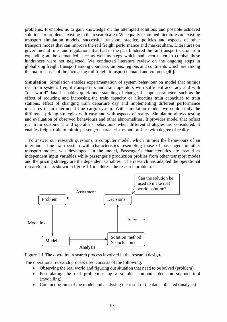
Simulation: Simulation enables experimentation of system behaviour on model that mimics real train system, freight transporters and train operators with sufficient accuracy and with “real-world” data. It enables quick understanding of changes in input parameters such as the effect of reducing and increasing the train capacity or allocating train capacities to train stations, effect of changing train departure day and implementing different performance measures in an intermodal line cargo system. With simulation model, we could study the difference pricing strategies with easy and with aspects of reality. Simulation allows testing and evaluation of observed behaviours and other abnormalities. It provides model that reflect real train customer’s and operator’s behaviours when different strategies are considered. It enables freight train to mimic passenger characteristics and profiles with degree of reality. To answer our research questions, a computer model, which mimics the behaviours of an intermodal line train system with characteristics resembling those of passengers in other transport modes, was developed. In the model, Passenger’s characteristics are treated as independent input variables while passenger’s production profiles from other transport modes and the pricing strategy are the dependent variables. The research has adapted the operational research process shown in figure 1.1 to address the research problem.

Figure 1.1 The operation research process involved in the research design.

The operational research process used consists of the following: Observing the real world and figuring out situation that need to be solved (problem) Formulating the real problem using a suitable computer decision support tool

(modelling) Conducting runs of the model and analysing the result of the data collected (analysis)

Problem Decisions

ModelSolution method (Conclusion)

Modeling

Analysis

Inference

Assesment

Can the solution be used to make real world solution?

- 11 -

Refining the model until results or behaviours which approximate the real entity it represents are obtained or observed (inference)

Conducting sensitivity analysis of the model Validating the model with reasonable or relevant real data.

The real world problem considered in this thesis is the problem described in section 2. The study focused on how the space utilisation and the performance of an intermodal line train cargo system can be improved using passenger production profiles and pricing strategies. Our first task was to find the train charge per ton-distance which can enable combined rail-truck transport competitive over all-road transport.

The study assimilates knowledge from economics, operation research, geography, mathematics, physics, logistics and computer science and its algorithms to create better solution to the existing rail freight problems. Knowledge from these areas was used to determine and evaluate different aspects and strategies that are used in our simulation model.

We also exploited the Nash Equilibrium concept, a widely used solution concept in the game theory [44], in the thesis. This concept guided us in determining the price relations between the truck and the rail transport freight mode. It assisted us in determining the price per unit ton-mile with which the freight train needs to operate in order to enable rail-truck transport more competitive. The main idea obtained from the Nash equilibrium which we applied in this thesis was the principle that in any game, if there are set of strategies with the property that one player can benefit to change his strategy while the other players keep theirs unchanged, then that player will always choice the strategy whose payoff will give him a maximum revenue compare to the others players. This concept was applied in tuning the cost per unit load-distance of the train, given that of the truck, obtained from literature, is fixed.

The study also make use of the commonKADS methodology [32] during the requirement specification phase of the study as it was suitable for acquiring in-depth knowledge and information which were needed in the design phase of our simulation mode.

1.5 Literature Review

A number of published literatures exist on the rail freight transport problems. There also exist tools on intermodal rail-truck freight transport. Many literatures address issues related to the forecasted growth in rail freight, the intermodality of rail freight, its falling market share, the operational, capacity and infrastructural adjustment which are needed to meet the expected future growth and demand in rail freight transport and other transport related problems. Some proposed means of combating the degrading rail freight market share. Most models on rail freight transport are oriented toward train schedules, forecasted growth, terminal operations and functioning, railway planning, resource allocation, loading/offloading operations and railway infrastructural [69]. Important literatures connected to this study include:

Pinkston [3] which presented the growth demanded in rail freight transport and the expected factors which will hinder railroads ability from meeting the future freight growth. According to Pinkston, investment in new tracks and equipment are needed for the rail freight transport mode to meet the rapid future freight gowth if it continues for 20 years. To her, the current situation of the rail freight transport mode could have been worst if there were no spread of Governmental policies to other modes of transport.

- 12 -

Bärthel and Woxienius [6] compared the capabilities of the conventional European road-rail freight transport (large flow over long and medium distances) with respect to the market nature and structure of freight flows. They explored possibilities of improving the conventional European intermodal transport through adapting into the Convention principles similar to those of passenger transport which can overcome accruing extra cost and time during pre-and post-haulage or drayage (cost before and after the haul) and during transhipment in a combined modes of transport over short distances. Illia and Laura [10] examined the possibility of increasing the market share of the rail freight mode in an intermodal transport chain using dedicated or semi-dedicated subnetwork for rail freight. According to them, increased rail freight market share cannot be achieved in a combined passenger-freight rail operation as are done by some rail operators. This is because operators shall always give more priority to passenger services than freight services. They foretold that increased rail freight market share and greater economies of scale would be achieved if innovated hub-and-spoke rail network structures similar to those of the air transport mode with regular and frequent schedules are dedicated to rail freight transport.

Taylor et al [5] studied the operational selection of intermodal ramp (region where rail load are transferred into truck road) within a rail-truck intermodal drayage movement. To them, assigning a ramp in a rail-road delivery process depends on the inbound and outbound rail ramp compare to the origin and destination of freights. EUFRANET project [12] identified and evaluated strategy options which can strengthen a Trans-European rail network dedicated to freight transportation. The project searched and proposed solutions and principles which can bring to the network an improved freight transport qualities and services with reduced freight cost, improved transport organisation and interoperability. The project also identified and evaluated new rail technologies which may enable economics and social growth of Europe through exchange of goods in an improved rail and intermodal freight transport system which is cost effective and environmentally friendly. A similar evaluation was conducted by Ballis and Golias [13] on the technical and logistics development which can enable an increased economic, technical benefits and effectiveness to railroad transport terminals. Their evaluation were based on the length and the effectiveness of using a transhipment tracks, train/truck arrival behaviours, types and numbers of handling equipments, mean stacking height of the storage areas, terminals access system and procedure. Chen et al [47] used yield management system to determine how the profitability of a competitive airline industrial can be improved. To them, the profitability of any competitive airline industry depends on a good yield management policy.

Morlok and lazar [22] studied approaches which enable improved combined railroad services. In their study trucks were used to pick freight from shippers to intermodal terminals and from terminals to customer at customers´ convenient time while rail hauled the freight from terminals to destination. Carey and Carville [23] studied the planning or scheduling of trains in a busy and complex train station where there are multiple operators with different and conflicting goals. Their aim was to draft train schedule which gives optimal satisfaction to train operators even though their goals conflict each other. Johanna törnquist [54] studied railway traffic disturbance management using re-scheduling policy which minimizes multiple stakeholders conflicting goals. To her, disturbance in railway traffic can be minimised if railway stakeholders can diagnosis their traffic and network using disturbance-related information. She equally suggested that disturbance management in railways traffic could beimproved if sustainable connection or trains prioritisation are eliminated in railways.

Belobaba [33] and Peng-Sheng [39] formulate and analyse a dynamic programming model of an airline seat allocation and other perishable commodities on a singled-leg flight with

- 13 -

multiple fare classes in situation where there is overbooking, cancellation and no-show (some passengers do not turn up for their booking order). Weatherford and Bodily [34] used mathematical programming to classify essential objectives (revenue, capacity utilisation, customer’s utility, operation, finance and market constraint) which need to be optimized in order to maximise revenue. Kimes [36] decomposed an airline revenue management operational policy into demand forecasting, Overbooking, Capacity allocation determination (seat inventory control) and pricing.

Clifford [70] developed an intercity freight transport model which can enable railroads to improve its services in an intermodal transport services. He was motivated by the facts that reliance in aggregate transport structure obscured clear observation of different shippers and customers behaviours. Guglielminetti et al [65] presents an optimization model for planning effective rail freight services through an effective, rational and customer-oriented approach. Their designed model was used to determine freight trains frequencies from estimated demand and route of freight movement which minimised cost. Higgins et al [67] designed an optimization model of train schedules on single-leg which provides optimal real train schedule and which enables changes in train schedules to be evaluated. Kraay [71] presents a model on fuel saving techniques which improved train performance with train satisfying the time window for their departure and arrival at train stations. Lee and Hersh [37] designed a stochastic control model which enables passenger pricing to depend on the available seat within a travel leg in a horizontal planning situation where the transport fare depending on the booking time. Kraft [24] designed a model that enables rail operators to achieve delivery time appointment in a railroad shipment with an optimal satisfaction of freight customer needs as well as the available and forecasted train capacity.

Ferreira and Sigut [72] simulate the conventional road/rail container transfer facility. They stressed the needs to closely monitor and optimised the performance of transport terminal with respect of customer services and operational efficiency. Boese [73] developed a simulation tool with several program modules that simulate the functions of a railroad terminal. He highlighted on the needs to use computer tool in the functioning of railroad intermodal terminals. Rizzoli et al [64] presents an agent-based simulation model of an intermodal flow among inland intermodal terminals which are interconnected by rail corridors. Timothy et al [61] uses discrete events simulation to model railway component of an intermodal operation. Sanjay and mark [14] examined a model which simultaneously optimizes facility location within a designed transportation network. Their model was used to analyse potential transport planning situations like transport resource allocation between facilities and links as well as the transport budgeting and planning decision within a simple classical plant location. Their study was motivated by the fact that change in network topology is more cost efficient than adding facility to improve the existing services.

1.6 Why Combined Rail-Truck Freight transport

All intermodal network points are linked by the road networks which facilitate the collection of freights from and/or to the nooks and crannies of the points. According to Woxenius and Bärthel [15], a rail-truck freight transport system in Europe is a universal solution to the numerous road freight transport and financial problems of many European national railways freight operations whose cost is approximately £ 250 million per year. A majority of these effects are from road congestion. Rail-road freight transport acts as a means of reducing the increasing freight traffic in cities and freight gateways (e.g. ports, terminals) more especially as trades are rapidly crossing national and international boundaries. The road freight transport

- 14 -

system, the main stream of inland freight transport, is highly congested and are having several infrastructural limitations which make it inextensible to accommodate the drastic increasing freight transport demands and volumes [7] [26]. In many cities, Lorries spend more than 10% of their operating time in congested or idle state [16]. The environmental impacts and economic losses incurred by Lorries at these states are substantial [17]. Road congestion impedes significant impact on the transport cost, efficiency of truck as well as the reliability of the just-in-time shipping policy which many shippers are fight to meet [19] [43]. In many regions, road congestion and environmental policies discourage further expansion and development on the road transport structures. These, therefore, called for alternative means of freight transportation or combined mode of transport which can minimise these negative effects of the road freight transport.

Also, globalisation and internationalisation of the transport industry with aims of facilitating freight transportation among countries and unions as well as integrating the fragmented, segmented and un-integrated transport modes (intermodal transport mode) and improving freight movement and volumes demand an improved freight transport between or among modal means of transport. Integration of the transport modes, the main focus of the transport industry, needs active and effective participation of all modal means of transport. Transport intermodalism won’t be beneficial to transport operators and freight transporters if transport services are poor and unequal among transport modes or if there are freight traffic and imbalance at intermodal network points. These, therefore, demand a strong binding force within modal operations as well as a strong intermodal relationship and operations of which the rail-road freight operation is among. See also [40].

Moreover, rail transport presently offers significant environmental advantages over other modes of transport. The gaps become much wider as electric tracks, which make rail transport more environmental friendly, are being introduced into the sector. Using the rail transport mode or combining it with other transport modes will bring substantial reduction to the degrading nature of our environment.

Combined rail-truck transport provides greater economics of the rail and truck hauled with reduced transport cost along the intermodal transport chain. Rail-truck transport leads to increased frequency of truck and rail services and the reliability of freight delivery processes. This enables the combined process to approach the just-in-time delivery process which is needed by freight transporters. Just-in-time delivery process enables reduced inventory holding and transport cost as well as an improved productivity of the economic of our system [45].

1.7 Limitations

Although this seems fruitful, it is challenging to implement a model of a line cargo train system with production profiles resembling those of passengers in other transport modes. This is because freights have a number of complex and interdependent characteristics which differentiate it from passengers and which make its transport difficult when using operational policies and technologies similar to passenger transport. These characteristics are logistics cost, commodity, shipment, mode of transporting the freight and loading and offloading time [20].

Logistics Cost: “The costs of moving freight are harder to determine compared to passenger moving since specialized services such as handling, loading, unloading, classifying, storing, packaging, warehousing, inventorying are required for freight transport” [20]. Difficulty in determining freight transport cost are also due to lack of standardised freight measuring unit,

- 15 -

more especially in international freight transport. Freight measuring unit differs among freight types and countries. Freight costs are determined from the quality of mass, bushel, weight(tonnes), (intermodal transport unit) ITU, TEU (Twenty Equivalent Unit), truck or vehicle units, values, boxes, etc. some of these units are hard to quantify. According to Yan et al [28], of the materials that existed on intermodal operations, none presents an effective way of estimating opportunity cost in rail intermodal freight transport. The worst cases are long term pricing policies with needs to forecast demand, economics growth, and future development and company conditions.

Shipment: There are no standardised units for measuring freight. Freight can be calculated in different money value, quantity, weight, volume, container, carload, truckload etc.

Commodity: Many types of commodities made up freight traffic. These commodities have a wide range of values and prices. Some are perishable items that need immediate or urgent transport while others are non-perishable or mixture. Some are liquid, gaseous or solid or mixture of solid, liquid or gas and types may demand separate handling, storage and packing.

Mode: “decisions by shippers, carriers and receivers affect whether or not a particular shipment should be made and, if so, by what mode and route” [20]. In passenger transport, passengers exercise free choice of transport modes, class (transport condition), road, etc but in freight transport, most decision regarding the freight class, the road to use, freight classification, transport mode, etc are made by the transporters not the freight owners. Most decisions involved group of persons with conflicting goals

Loading and Off-loading Time/process: The loading and off-loading processes involved in freight transport are time consuming, personnel intensive and cost-intensive compare to passenger transport.

1.8 Outline of the thesis

In the next chapter, we describe the research problem as well as some aspects of modelling, while in chapter 3, we outline our model choice, reasons to develop a tool rather than using a standby developed tool. We also described in chapter 3 the different entities that are modelled, their attributes and implementation. Our simulation experiment description is also presented in this chapter.

In chapter 4, we present our data and their sources, the model verification, validation, sensitivity analysis and the results of the simulation conducted and their analysis.

We present in chapter 5 a summary of the result achieved and finally suggests on possible improvements of the thesis in chapter 6.

- 16 -

2 Problem Description and modeling

We shall implement a computer model of an intermodal line cargo train system which describes the following in figure 2.1:

Figure 2.1 Customer requests for rail transport service.

Freight transporters place transport request to the train operators. The train operators evaluate the transporter transport cost through the combined system(rail-truck system) and send to the transporters who compare the cost with their direct cost of transporting the freight from origin to the destination using all-road truck. Result of the freight transporters comparism are sent to the train operators indicating their preferred transport mode. If the decision is that the transporter want to use the combined system for their freight transportation, the operators offer the transporters the transport service. The following shall be consider in the thesis:

2.1 Customers and accepting the transport offer

We shall look at situation where there are freight transporters(customers) who have freight to transport from freight locations to the freight destinations. Customers appear (Call the train operators to place transport order) within a time window before the departure day. They appear one at a time. Each customer is characterised by the location (origin of his goods or where his goods is currently located and a destination (final point where his goods is moving to), location of shipment address (closest / agreed start and end train stations), knowledge of direct transport and its cost, preferred transport means (direct transport or transportation through rail-truck system), preferred departure day and the transport request placement day (the day he booked transport order). In general, they exercise free choice of start and end train stations i.e. they choose closest train stations to their freight locations and destinations as their start and end train stations. Through an agreement with the train operators, they may change their preferred train stations and departure days. We model the agreement to change preferred train stations as cases where their freight can not be accommodate on the train between their closest train stations during the departure day or cases where their closest stations do not give transport cost advantage over direct all-road transport. Customers transport their goods to/ from the preferred/agreed start and end train stations. They decide to transport goods (willing to pay the

Customerrequest Operators

Request transport

Offer transport service (including price)

Decline or accept transport offer

- 17 -

price offered if train price give transport advantage over all-road transport) or may refuse (if train price does not give transport cost advantage over all-road transport). Their willingness or preparedness to pay for the price offered or to choose direct freight transport depend on which is cost advantage, direct transport of freight from origin (current freight location) to destination (freight destined point) or the cost of transporting the goods from current freight origin to the customers´ preferred/agreed start train station (using truck) plus the price they are offered by the train operators for transporting the goods from the start to the end train station (using train) plus the cost of transporting the goods from end train station to freight destination(using truck). They accepted the combined rail-truck transport when it provides transport cost advantage for transporting their freight or choose direct all-road transport when the combined rail-truck transport does not provide cost advantage for transporting their freight. The transport decision made by the customer is shown in figure 2.2.

Figure 2.2 Customer decision on the transport mode to consider

2.2 Transport routes or options the customer examined

Each freight transporter is faced with the following route options in figure 2.3. The transporter solution to this route problem enable him to decide which tranport option he should consider.

Figure 2.3 Transport routes or options the customer examined

Freight destination

Train

B C D E

Freight origin

truck

truck

Direct truck

customer Accept Rail-truck transport

Consider direct all-road truck

Send priceEvaluates and decides

- 18 -

Freight transporter determine if it is possible for them to transport their freight from freight origin to freight destination through the routes: freight origin to train station B(using connection truck ), from train station B to train station E(using train) and train station E to freight destination (using connection truck) or they should consider the route freight origin to train station C(using connection truck), train station C to train station E(using train) and train station E to freight destination(using connection truck) or from freight origin to train station B(using connection truck), from train station B to train station D(using train) and from train station D to freight destination(using connection truck) or they should consider freight origin to Train station C (using connection truck), from train station C to train station D (using train) and from train station D to freight destination (using connection truck) or they should transport their freight direct from freight origin to freight destination(red line) using direct all-road truck. What determine the route a freight transporters should consider is his freight accommodation within the train stations and his transport cost compare to direct all the road freight transport. A customer immediate consider transport through the train if a travel leg is found that can provide him load accommodation with transport cost advantage else he consider the direct all-road transport.

Each customer has the option of transporting his freight through a combined rail-truck transport or direct all-road transportation of freight. As is in Fig 2.3, when a customer calls the train operators to book transport order (request transport in figure 2.1 above), the train spaces within his chosen travel sub leg are examined if they are space to accommodate his load. The operators evaluate his transport cost within his travel sub leg if there is space to accommodate the load on the train within the travel sub leg. In general the operators evaluate his transport cost between the closest train stations to his freight location and destination and send to the customer. The customer compares this cost plus other cost that will be incurred in connecting the freight to and from the train stations (entire cost through the combined rail-truck system) with the direct cost of transporting the freight from freight’s origin to destination. But in our model, we model as the operators evaluate the customer transport cost through the combined system and compared it with the direct cost of all-road transport. If the cost of transporting the freight through the combined rail-truck system is less than the direct all-road cost of transporting the freight, the customer considers the combined rail-truck transport offer else the direct all-road transport. In cases where the customer load cannot be accommodated between the closest train stations to the customer’s freight location and destination, the operators search as in figure 2.3 above other train stations during the customer departure day or other departure days which can accommodate the customer loads. If train stations are found that can accommodate the load with transport cost advantage compare to the cost of transporting the load directly from freight origin to freight destination using direct truck, the customer consider the combined rail-truck transport offer. When no train stations are found that can accommodate the customer freight with transport cost advantage over all-road transport or if train stations are found that can accommodate the load but can provide the customer transport cost advantage over all-road transport using direct truck, the customer consider direct all-the-road transport of their freight.

2.3 Transport services offered by the train and truck.

In our model, we shall consider situations where freight train is allowed to stop at relatively few number of train stations for rather quick loading and unloading of cargo. A train or truck is used between train stations depending on which mode provides transport cost advantage and the train loading and offloading time at the stations. Trucks transport freights from freight’s location to the train stations and from train stations to freight destinations. Either a truck or a

- 19 -

train transport freight between train stations (from one train station to another). We assumed freights are directly transferred from connection truck to the railcar and vice visa at the intermodal network point. Train follows a fixed schedule while connection trucks departure and arrival adapt to the train schedule. Train has a fixed capacity which changes as cargoes are allocated on it. Each train stations have a fixed loading space (equal full train load) on the train which reduced as load are accepted at the train station and at other train stations before it, provided the freight have to pass through it before its offloading train station. Before each customer load is accepted for rail-truck transport between the train stations, the current available train space at all train stations through which the load will pass before its offloading train station are checked if they can accommodate the load. This is to ensure that freights are not accepted than the train can carry at any train station along the travel leg. This is achieved by ensuring that before loads are accepted between any train stations, the load must be less than or equal to the minimum available train space along the leg i.e. the minimum current available train space at all train stations between the loading train station and the offloading train station. Trucks are assumed to be available whenever and wherever needed. Freight transporters (customers) transport their freight from freight origin to the accepted or closest start train station and from the accepted /closest end train station to the freight destination.

2.4 The Prices the Train Operators Offer

We shall examine two pricing strategies with our developed model. These are the dynamic and the constant pricing strategies with train capacity allocation and the provision of alternate train station to freight customers. The dynamic pricing strategy is later compared with a constant price strategy which we consider as our base test scenario.

2.4.1 Constant Pricing Strategy

In constant pricing strategy, price is calculated disrespect of the transport order placement day, the available train capacity and the travel sub leg. Prices do not depend on the current available train space within travel sub legs. Customers pay the same train price per unit cargo-distance (price per unit) if their load would be accommodated on the train between any train stations or during a departure day. The price depends on the distance between the start and end train stations and the quantity of freight the customer has to transport between the train stations. The train price per unit cargo-distance is unaffected by change in train stations or departure day but rather by the distance between the stations within which the freights will be accommodated on the train during the accepted departure day. The constant pricing strategy is a base scenario in the dynamic pricing strategy. It is the minimum price a customer will pay during dynamic pricing when train capacity is unlimited.

2.4.2 Dynamic Pricing

Dynamic pricing strategy is adopted from the airlines and passenger trains where it forms the operating principle of the yield management system [27] which is used to price passengers based on the available capacity and the booking time. It has as a base price level the constant price strategy. During the dynamic pricing strategy, freights are priced depending on the minimum available train capacity along a travel sub leg and the time a customer books transport order. The train price per cargo-distance depends on the available train space and the time of booking transport order from the train departure day. Dynamic pricing is the function of the current minimum available train capacity with travel sub leg, time of booking transport order, distance and load. It dynamically changes and depends on the day customers place

- 20 -

transport order and the available train space within the travel leg. It increases/decreases as the train departure day approaches depending on the transport demand and the available train space. The Price depends on the start and end train stations i.e. the distance between the preferred/agreed start and end train stations of a customer. It also depends on the transport sub leg. This is because the minimum available train spaces among the different travel sub-legs when customer appears to book transport request are not the same. For this reason, the price paid by customers who have the same load and who booked transport order on the same day for the same train departure day between different travel leg differ depending on the minimum available train capacity within their travel sub legs. In some cases, customers who booked transport order long before train departure day when the train capacity are not limited pays the same prices as those who booked order few days to the departure day depending on the transport demand. This is in situation where the departure day has almost approach without the operators haven’t obtained enough trainload. Here, the operators offer relatively low price (the base price level) to the customer in ordered to obtain enough trainload. In such case, they price the customer disrespect of the current available train capacity within their travel sub leg. These low prices (price offer to obtain enough trainload) are the constant price the customer will pay if all customers were price uniformly (disrespect of the available train space and the transport order request day) and are properly estimated to minimize lost opportunities in total operator’s revenue. This is the marginal cost which depends on customer’s choice. Customer who wants urgent transport may pay additional transport cost depending on the space and the day they want the service. Customers whose loads are accommodated during departure day other than their preferred departure days may pay high, less or the same price than they could if their loads were accommodated during their preferred departure days. This is because of the dependent of the prices on the transport request placement day from the train departure day.

2. 5 Transport Scheduling

The train operators scheduled train departure days i.e. departure days from the first train station. This depends on their permission to use the rail track by other train operators on the network. They decide on the possible train stations the train should stop for quick loading and unloading of freights. This depends on the loading and unloading time at the train stations, the train stopping time at the stations and the transport cost incurred when using train or truck between the train stations. The choices of the stopping stations are purposefully to reduce transport cost (maximized revenue through cost minimisation). Another prime goal of selecting train-stopping stations is to reduce train delay and other irregularities that may prevent the train from meeting schedule. It is also purposefully to provide freight customers transport services at their convenient time. Operators calculate the freight prices, determine if there are available train capacity for the customer freights, negotiate with the customers to used later train (later departure days) or train stations and decided where to use the truck along the leg.

Another cost determines using the model is the train price per unit ton-distance. This is obtained using our developed through tuning i.e. holding the truck cost per cargo-distance, which is obtained from literature, fixed and tuning that of the train at different price levels to find a good train operating rate per ton-mile which will enables the combined rail-truck services competitive over all-the–road transport. The tuning is conducted with the constant pricing strategy since it appears partly in the dynamic pricing strategy.

- 21 -

3 Modelling and Implementation

3.1 Model Choice

We need to model the problem in order to perform the analysis. We need a suitable choice model and method to model the problem since different computer model simplify, abstract and analysis reality differently. A suitable model to any problem domain depends on how it captures and relates the domain variables (decision variables, controllable and uncontrollable variables). Very crucial for any model is its ability to model the variability inherent of the real system it represents. A good model to represent any real domain must be capable of providing a balance in the problem simplifications and its representative requirements so that it captures enough reality within the problem domain.

According to Vita et al [74], traditional mathematical modelling and simulation techniques dominate for optimisation solutions of the transport domain which is complex and involves large entities and resources. From Garcia et al. [2], rail freight transport systems are complex and require techniques to assist the operational and planning processes. It appears impossible to capture transport modes or vehicle choice in the transport system (Swaminathan et al [59] and Strader et al [60]). According to Macharis et al [55], intermodal transport is a complex system with characteristics difference from other transport system. Multiple nonlinearities, combinational relations, complex nature and uncertainties in intermodal freight system variables have made our problem suitable for simulation [66]. This is because of its suitability in capturing and modelling the real entities involved (customers, train, trucks and transport operators) and their characteristics. Simulation provides an effective approach to analysis and evaluate the transport chain, transport strategies and to manage decisions within the transport chain [58]. Simulation has the capabilities of modelling physical processes within the transport chain with incorporation of uncertainties that are inherent to real transport systems. It provides advantage in analysing situations with too complex mathematical formulations. It provides virtual experimentation of different transport policies and alternatives that affect physical real entities. It enables easy prediction of real transport system characteristics under different conditions. It allows best of several transport alternatives to be selected through experimentation. Transport options and strategies can be implemented quickly using simulation since the relationships among components in a simulation model are mathematical modelled. Simulation allows what-if analyses and enables bottleneck identification. The important of simulation in relation to handling our problem domain can be understood in [50] where Van Der Heijden used object-oriented simulation to design an automated underground freight transportation system which enables road congestion problems around Schiphol Airport to be studied. It is worth noting that this couldn’t have been achieved using other computer modelling tools as they could not capture the complex variables that were needed for the system. We are therefore considering simulation as a suitable tool for analysing the performance of an intermodal rail-truck system since complex price relationships of the different transport modes and the combined complex structures form combined rail-truck transport chain can be modelled effectively.

- 22 -

3.2 The Developed Simulation Model

Our choice of building our own simulation model rather than using a standby model was because most existing transport models are modal oriented or microscopic in scope with none addressing issues on the performance of a combined transport system (Tan et al [62]). Moreover, most existing transport simulation tools do not support modelling and analytic features that are required for our situation (Andradottir et al [75]).

The simulation model is implemented in C# (C sharp) computer programming language download online from MSDN (Microsoft Developer network), provided for free to students, researchers and software developers by Microsoft. The particular choice of C# was because of its numerous advantages in using and handling array, more especially multiple array inheritance. Advantage in defining value types using enumeration which can be treated as C# predefined type, defining and using with easy new references using class, interface and delegate [30] are also reasons why we considered C#.

In our simulation model, we have modelled the train stations, train operators, customers, train and trucks. These entities are implemented in the model as follows:

3.2.1 The Train Stations

The train stations have the following attributes:

Location: Each train station has coordinates which correspond to its geographical location. In the simulation, we considered 10 train stations. These stations are number in ascending order from 1 to 10.

Maximum Train Capacity: Full trainload is the maximum quantity of freight which can be accepted at any train station. The freights accepted at other train stations before a train station may affect the quantity of freights that can be accepted at a train station. Train stations whose trainloads are affected by freight accepted at other train stations are stations which fall between the start and end train station of the accepted freights. This is because the accepted freight will remain and occupy the same space on the train until the end train station is reached where there are unloaded. For this reason, the loading process at each train station takes into consideration the current available train space at all train stations where the freight will occupy space on the train before there are unloaded. This is to avoid more freight than the train can carry at any train station. To ensure this, freights are accepted within a travel sub-leg if there are less than or equal to the current minimum available train space within the travel sub-leg. For this reason, the maximum trainload at each train station depends both on the freights accepted at that train station and those accepted at other proceeding train stations i.e. freight accepted from customers whose start and end train stations appear before and after the station. At the start of every simulation, all train stations are assigned a maximum load capacity equal the full trainload. When a customer accept the price offered, the current available train space at all train stations from his start train station to the train station just before his end train station reduced by an amount equal the quantity of freight that customer have to place on the train.

Train Station Load and Offload: A Train Station load is the total quantity of freights that have been accepted at the train station or that have been received from customers at a train station to transport to other train stations after the train station. It is the total quantity of freight that will be

- 23 -

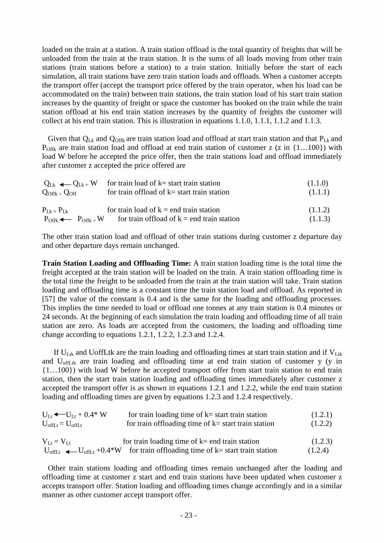
loaded on the train at a station. A train station offload is the total quantity of freights that will be unloaded from the train at the train station. It is the sums of all loads moving from other train stations (train stations before a station) to a train station. Initially before the start of each simulation, all train stations have zero train station loads and offloads. When a customer accepts the transport offer (accept the transport price offered by the train operator, when his load can be accommodated on the train) between train stations, the train station load of his start train station increases by the quantity of freight or space the customer has booked on the train while the train station offload at his end train station increases by the quantity of freights the customer will collect at his end train station. This is illustration in equations 1.1.0, 1.1.1, 1.1.2 and 1.1.3.

Given that QLk and QOffk are train station load and offload at start train station and that PLk and POffk are train station load and offload at end train station of customer z (z in {1…100}) with load W before he accepted the price offer, then the train stations load and offload immediately after customer z accepted the price offered are

QLk QLk + W for train load of k= start train station (1.1.0)QOffk = QOff for train offload of k= start train station (1.1.1) PLk = PLk for train load of k = end train station (1.1.2) POffk POffk + W for train offload of k = end train station (1.1.3)

The other train station load and offload of other train stations during customer z departure day and other departure days remain unchanged.

Train Station Loading and Offloading Time: A train station loading time is the total time the freight accepted at the train station will be loaded on the train. A train station offloading time is the total time the freight to be unloaded from the train at the train station will take. Train station loading and offloading time is a constant time the train station load and offload. As reported in [57] the value of the constant is 0.4 and is the same for the loading and offloading processes. This implies the time needed to load or offload one tonnes at any train station is 0.4 minutes or 24 seconds. At the beginning of each simulation the train loading and offloading time of all train station are zero. As loads are accepted from the customers, the loading and offloading time change according to equations 1.2.1, 1.2.2, 1.2.3 and 1.2.4.

If ULtk and UoffLtk are the train loading and offloading times at start train station and if VLtk

and UoffLtk are train loading and offloading time at end train station of customer y (y in {1…100}) with load W before he accepted transport offer from start train station to end train station, then the start train station loading and offloading times immediately after customer z accepted the transport offer is as shown in equations 1.2.1 and 1.2.2, while the end train station loading and offloading times are given by equations 1.2.3 and 1.2.4 respectively.

ULt ULt + 0.4* W for train loading time of k= start train station (1.2.1)UoffLt = UoffLt for train offloading time of k= start train station (1.2.2)

VLt = VLt for train loading time of k= end train station (1.2.3) UoffLt UoffLt +0.4*W for train offloading time of k= start train station (1.2.4)

Other train stations loading and offloading times remain unchanged after the loading and offloading time at customer z start and end train stations have been updated when customer z accepts transport offer. Station loading and offloading times change accordingly and in a similar manner as other customer accept transport offer.

- 24 -

Train Stopping Time: To each station is the train stopping time. This is the time the train takes to stop (the time train takes to fully came to rest for loading and offloading processes to comment at a train station) and to leave (the time train takes to steam up and leave the train station after breaking). Train stopping time at each train station depends on the loads the train arrives and leaves with at the station. In the simulation, we assumed a train which carries no load takes is 5 minutes (estimated value) to stop or leave a train station. An empty train will take 10minutes (5 minute for stopping and 5 minute for steaming and leaving the train station) to decelerate to zero speed at a station and to steam up and leave a station. The train braking time is 5 minutes plus beta times the load the train arrives with at the train station. The value of beta as reported by [31] is 0.00009 and is the coefficient of the additional frictional force exert by each tonnes place on the train on the rail track. The value (0.00009) differ from what is found in literature [31] because in [31] the weight are measured in Kilo tonnes while in our simulation freights are measure in tonnes.

On the other hand, the time the train takes to steam and leaves a train station is 5 minutes plus beta times the load the train leaves the station with or it is beta multiples by the sum of the load the train arrives the train station with and the load the train carries at the train station minus the quantity of load unloaded at the station plus 5 minutes.

The train stopping time at any station is the sum of 10 minute plus the braking time plus the time the train takes to steam and start moving.

Total Braking Time at a Train Station (TS): This is the total time incurs by the train when it stops at a train station. It is the sum of the offloading time, loading time and the train stopping time, It is calculated as TS= 10 + beta*(2* total load the train arrive with at station – station offloading quantity + station loading quantity) + station offload time +station loading time (1.2.5) Or TS = train stopping time + loading time + offloading time

Determining the total train breaking time at the train stations was purposefully to determine where along the singled-leg a truck should be used in order to reduce train delayed. Train passes without stopping at train stations with large braking time while trucks are used between such train stations.

3.2.2 The Customers

There are implemented as objects with characteristics resembling those of real customers. During the simulation, each of these objects acts as a process that performs a task (book transport order) in the operating system. Their behaviours are alike as the real train customers who call the train operators to place or book transport order. Each customer has characteristics stored in a multiple dimensional array from where there are retrieved by the system for examination. These characteristics include:

Customer Location: In the model, each customer has a location which is the geographical points (coordinated points) where his freight is located and moving. The freight current

- 25 -

locations are described in the model as the customer origins or freight origin (where the freight is currently located) and the freight destinations (called destination in the model) is the destination of the freight. Each customer origin (freight current location coordinate) is obtained by randomly generating a number from one to eight and his destination is obtained by randomly generating a number from the seventh geographical point from his origin and 15 i.e. a customer origin is a random generated number among 1 and 8 while his destination is a randomly generated number from his origin + 7 and 15. These numbers have pre-assigned coordinates. The choice of obtaining the destination by randomly generating a number a seventh geographical point from the origin and 15 is to discourage short distance train freight transportation which gives more preference to direct transport of the freight from origin to destination (in term of transport cost) than transporting the freight through the combined rail-truck system [46].

Customer Start and End Train Stations: Associated to each customers are the train stations (start and end train stations) where they transport their freight to using connection truck if they accept the price offered by the train operators and from where they collect their freight for further transportation using connection trucks to the freight destination. Customer’s start train station (station they transport their freight to if they accept the price offered and if their load can be accommodated on the train) are the closest train station to their freight current location and their end train stations (where they collect their freight from the train operators) are the closest train station to their freight destination. Start and end train station are the closest train station to the customer’s origin and destination that can accommodate the customer freight with transport cost advantage. The closest train stations to the freight origin and destination are determined by the system. The system uses search algorithm to find among the train stations the closest train station to each customer origin and destination.

Customer Load: Customer load is the quantity of freight a customer has to transport. The customer’s load are obtained by randomly generating number from 20 to 100 and stored them in an array at the beginning of each simulation. Customer load can either be accepted between some train stations during a departure day or rejected if it cannot be accommodated between train stations during his departure day or between closest train stations during 3 other available departure days from this departure day (if his departure day is not the last train departure day in the schedule). His load is also rejected if rail-truck transport does not provide the customer transport cost advantage over all-road transport. Customer load can be accommodated on the train at a train station if the load is less than the minimum available train capacity within the travel sub leg i.e. if his load is less than or equal to the minimum of the current available train space along his travel sub leg (minimum of the available train space for all train stations which lies from his start or agreed start train station and the train station just before his end or agreed end train station. This is normally the train stations capacity before his load is placed on the train.

Departure Day: Each customer has a departure day which is the day before which his freight will be available at the start train station. It is the day his freight is transported from his start train station to his end train station. It is the day he collects his freight at his end train station. In real world this is normally what happen but in our model, the system randomly generates each customer departure day among the available departure day. In the model, freight transports are done from Monday to Friday i.e. a Customers departure day is a day among Monday to Friday. A Customer departure day may change if his freight can not be accommodated on the train or does not gives transport cost advantage over all-road transport during this departure day. All departure days have pre-assigned date.

- 26 -

Transport Order Request Placement Day: Each customer has as a characteristic the day he called the train operators to place transport Order (transport order replacement day). This day is a randomly generated day among days from the transport schedule day to the customer preferred departure day. In the model, the computer system pre-assigned the transport schedule day at the beginning of each simulation. It also pre-assigned the departure days at the beginning of each simulation. Transport Order request placement Day is a day randomly generated from the assigned transport schedule day to the departure day. For example, if a customer has Monday as his departure day then his Transport Order request placement Day is a random generated day from the assigned transport schedule day to Monday. This day is vital for calculating the customer transport cost and in limiting the train resources to the customers more especially during dynamic pricing. The train cost per unit cargo-distance during dynamic pricing strategy depends on the different between Transport Order request placement Day and the departure day and the available train capacity.

Transport Offer Acceptance: For a customer to accept the price offer, the following must be satisfied:

1) The customer freights must be accommodated on the train within a travel sub leg or during a departure day

2) The price of transporting his freight through the combined rail-truck system must give the customer transport cost advantage compare to transporting the freight directly using direct all-the-road transport truck.

Customer load is accommodated on the train if it satisfies equation 1.3.0 below. In addition to the customer load been accommodated on the train, the transport cost of transporting his freight through the combined rail-truck transport service should give the customer transport cost advantage over all-road truck. When a customer load can be accommodated, the system, calculates the customer transport cost from his start train station to his end train station. Customer compares the cost offered by the train operators plus the connection costs that will be incurred in transporting the freight from freight origin to his start train station and from his end train station to the freight destination with the direct cost of moving the freight from freight origin to the destination using direct all-road transport. Customer compares the cost of transporting the freight from freight current location to the start train station using connection truck plus the price offered to him by the train operator plus the cost of transporting the freight from end train station to the freight destination (using connection truck) with the cost of transporting the freight from the origin to the destination using direct truck. The costs used for the comparison are Cost (origin, start train station) 1 + price (start train station, end train station)2

+ Cost (end train station, destination)3 and Cost (origin, destination)4.

3.2.3 The Train Operators

Train operators scheduled the train departure days in advanced before the loading period.They received transport order from customers (retrieved the customer transport request from the customer data stored in an array). They also perform the following functions in the model:

1 Transportation is done using the truck.2 Transport by train.3 Transport by truck. 4 Transport by truck.

- 27 -

Checking Customer’s Load accommodation: when each customer appears to place transport order, the operators check if there are available or enough train space within his preferred travel sub leg to accommodate this load. The check is as shown in equation 1.3.0.

If the current train capacity of train stations J to K are Cj, P>J, J, K in {1…10}, J and K are the start and end train station of a customer y with load L tonnes. Then his load can be accommodated on the train from train station J to K,

If minimum (Cj) - L >= 0 j in (J … K-1), y in (1…. 100) (1.3.0)

Searching Alternate Start and End Train Stations: If a customer start and end train stations (closest stations to the customer origin and destination) can not accommodate his freight or provide transport cost advantage compare to direct transport of the freight from origin to the destination using all-road truck, the train operators find other train stations between his start and end train station (closest stations) i.e. other train station closer to the freight origin, the freight destination or both, that can accommodate the freight with transport cost advantage compare to direct transport of the freight from origin to destination using all-road truck. In the model, three train stations closer to the customer start train station are first considered while the end train station is held fixed. If this does not provide train stations which can accommodate the customer freight with transport cost advantage compare to all-road truck transport, the start station is held fixed while three train stations closer to the end train station are tried. During the search for alternate train stations, the operators ensured that the start train stations are always train stations before the end train stations. If searching the end train station does not provide the customer a travel sub leg which can accommodate his freight with transport cost advantage, a combination of train stations from both the start and end train stations are considered. Three train stations from the closest start and end train stations are considered, provided there are three stations that lay between the customer start and end train station and that the start train’s stations are stations before the end train station. In all the cases, the search process terminates when a sub travel leg is found that can accommodate the customer freight with transport cost advantage. The searches take into account the fact that freight transport is unidirectional and thus, each customer destination is location after his origin. In any of these cases, if an alternate start or end or both are found that can accommodate the customer load with transport cost advantage, the customer start and end train start became the found train station(s). Generating Alternate departure Days: if during the train stations searches no travel sub leg is found that can accommodate the customer freight during his preferred departure day, the train operators check other departure days from the customer preferred departure day if there are train stations that can accommodate the customer freight with transport cost advantage. Three departure days are considered from each customer preferred departure day, provided there are three more departure days from the customer’s departure day in the schedule period. The day search stops when there is no more train departure day or if the customer departure day is the last train departure in the schedule. It also stops once a departure day is found that can accommodate the load with transport cost advantage. Whenever a departure day is found that can accommodate the customer’s freight with transport cost advanced over all-road transport, the customer departure day become the found departure day.

Update the train spaces: When a customer accepts the transport offer (i.e. when his load can be accommodated on the train with transport cost advantage), the operators update the available train space of all train stations from the customer start train station to the train station just before his end train station. This is to ensure that freight are not collected than can be accommodated on the train at any train station since the freight will occupy the same space or remain on the

- 28 -

train until it reaches the train station where it will be offloaded from the train. The updating process is thus through deducting the current available train space of all train stations that lay from the customer start train station to the train station just before his end train station by the quantity of freight the customers has to transport. The end train station is excluded because at such station, the freight will be unloaded and hence providing train space rather than occupying train space. The updating process is as shown in equations 1.3.2, 1.3.3, and 1.3.4.

If the current train capacity of train stations J to K are Cj, P>J, J, K in {1…10}, J and K are the start and end train station of a customer y with load L tonnes. Then, the available train spaces or capacities after the customer have accepted the transport offer are updated as

Cj =Cj –L j in (J …K-1) (1.3.2)

Ck= Ck k not in (J … K-1) (1.3.3) This is true for all train stations during the customer departure day. The train capacity remains the same at all other train stations during other departure days. That is during other departure days

Cj = Cj for all train stations during other departure day (1.3.4)

Updating the train space within travel sub legs enable the train operators to determine if capacity levels are reached within travel sub legs where the different pricing levels during the dynamic pricing can be used to pricing the next coming customers.

Calculate Customer Transport cost: The operators calculated the following prices which assisted the customer in deciding whether to use the direct all-road transport service or combined rail-tuck transport service.

Direct Price

The direct price is calculated as in equation 1.5

Direct price = F1 + DOD * (C + L*Cld) (1.5)

Where F1 is the truck threshold cost (cost of documentation, billing, loading, offloading, infrastructure cost). It is independent of the distance. DOD is the Euclidean distance from the freight’s origin to the freight’s destination. The distance is the direct distance between the two points. C is the truck operating cost per mile (vehicle maintenance cost, ownership cost, fuel cost, cost of using drivers and others). L is the load the customer has to transport and Cld is the cost per load-distance.

Constant Pricing

In the constant pricing strategy, all customers are priced disrespect of when they place the transport order and the available train capacity within the travel sub leg. All customers pay the same train price per unit cargo-distance, rail infrastructure cost and operating cost. The constant price is calculated as shown below.

- 29 -

Price (P) = F2 +DSE*(C1+L*Cld2) (1.6)

Where F2 is train threshold cost (i.e. a portion of the sum of the transfer cost and Flagfall charge. Flagfall is the fixed cost charged (infrastructural cost, registration cost) per train. The train threshold cost is independent of the distance. C1 is the train operating cost per mile (maintenance cost, ownership cost, fuel cost, cost of using drivers and others) and depends on the distance. Cld2 (obtained partial using the Nash equilibrium concept [44]) and by tuning, is the train cost per unit cargo-distance, DSE is the Euclidean distance from the customer start train station to his end train station. L is load.

Dynamic Pricing

Here, prices depend on the transport order request placement day from the departure day and the minimum available train capacity within the travel sub leg when a customer booked transport order. It also depends on the distance and the load the customer has to transport. Formulation of the dynamic pricing policy was based on the material presented in [35] which states that the optimal policy of a competitive airline depends on the state and is time dependent on the booking limit of each fare class. From this literature, a good freight pricing policy, which can enable rail-truck freight transport system competitive, depends on the available train capacity and the time the freight transporters placed the transport order. It is optimal to accept a low price cargoes and simultaneous reject a high price cargoes due to the loss in revenue that may be cause by the accepted high price cargoes. This implies it is a good to accept low price cargo that can be accommodated on the train than to accept high price cargo which may bring to the operators reduction in the total revenue. It is therefore reasonable to accept many low price cargoes that will give overall high revenue than to accept fewer higher price cargo which will give a gross lower revenue compare to the many lower price cargos that would have been accepted. This principle is inline with the Nash equilibrium concept which was mentioned earlier. The Cases below illustrate how the dynamic prices are calculated. The cases are derived from the material presented in [57], [37] and [38] on freight transport cost and passenger pricing.

Case 1

When a customer place transport order within 4 day to the departure day and when the minimum available train space along his travel sub-leg (current minimum available train capacity within his start and end train stations) is less than 20 percent of the initial train capacity (full trainload) then, his rail price is calculated as

Price (P) = F2 +DSE*(C1+L*(Cld2 + 0.01 * C3 )) (1.7.1) Where F2, DSE, C1, Cld2, L are as defined in equation 1.6 above. C3 is the initial train capacity (full trainload) divided by the minimum available train capacity within the travel sub leg.

Case 2

When the customer place transport order between 4 and 7 days from the departure date when the minimum available train space within his travel sub-leg is less than 40 percent of the initial train capacity, his rail price is given by

Price (P) = F2 +DSE*(C1+L*(Cld2 + 0.01 * C 3 )) (1.7.2)

- 30 -

Where F2, DSE, C1, Cld2, L are as defined in equation 1.6 above. C3 is the initial train capacity divided by the minimum available train capacity within the travel sub leg.

Case 3

In all cases different from cases 1 and 2 or when customer places transport order when the minimum current train capacity within his travelled sub-leg is above 40 percent of the initial train capacity. The price is calculated as in equation 1.6 above. The calculation is disrespect of the minimum available train capacity within the travel sub leg and his transport order placement day.

The Transport price formulations (both for the truck and rail prices) are based on the material presented on [58]. From the literature, the price of a transport mode consists of a Flagfall charge and a variable cost. The Flagfall charges are the mode infrastructure, administrative, transactional and other costs. It is a fixed cost charged on the entire mode i.e. per train or per truck. Spreading the fixed Flagfall charge over more tonnage reduces the cost per ton paid by the freight transporters. This is the reason why we have implemented this component of the cost as a fixed and equal charge that is paid by all customer disrespect of the load they have to transport. Other cost parameters added to the Flagfall cost is the transfer cost for the train transport mode, which is the cost of transferring the load from truck to the railcar or from the railcar to the truck at intermodal network points and the dray cost in the truck transport mode, which is the cost of billing, documentations, loading and offloading. The variable costs depend on the distance and the loads the customer have to transport. It includes the operating cost which depends on the distance and the cost per unit cargo-load which depends on both the load and the distance the load will be moved.

Checking where to use a Truck or a Train: Using a train or a truck between two train stations depends on the train braking time and the transport cost of the truck and train between the two train stations. In the model, we found that the train stopping time at the train station is the sole determining factor on using a truck or a train between the train stations. This is because the train transport mode provides cost advantage over truck freight transport at medium distances. The train stopping time stands as the determining factor on where to use a truck or a train between the train stations in our model. In the simulation, we assumed that for truck to be use between two train stations the transport cost, even though no significant, of using a truck between the stations should be less than the cost of using a train between the stations or the train stopping time between the stations should be greater than 300 minutes. We used large train braking time (value 300) in our simulation simple to discourage frequent truck usage between train stations since it is cost disadvantageous to the operators.

3.2.4 The Train/Truck

Train and truck are entities that transport freight from one place to another. Transportation of freight from freight locations to start train stations and end train stations to freight destinations are done by trucks (connection trucks). These are solely the responsibility of the customer. The prices incurred during connections are vital for determining which transport mode, rail-trucks or all-road transport, gives the customer transport cost advantage. Train or both train and truck transports freights between the stations during the departure days. A truck or a train is used between train stations depending on the transport cost and the train stopping time at the stations.

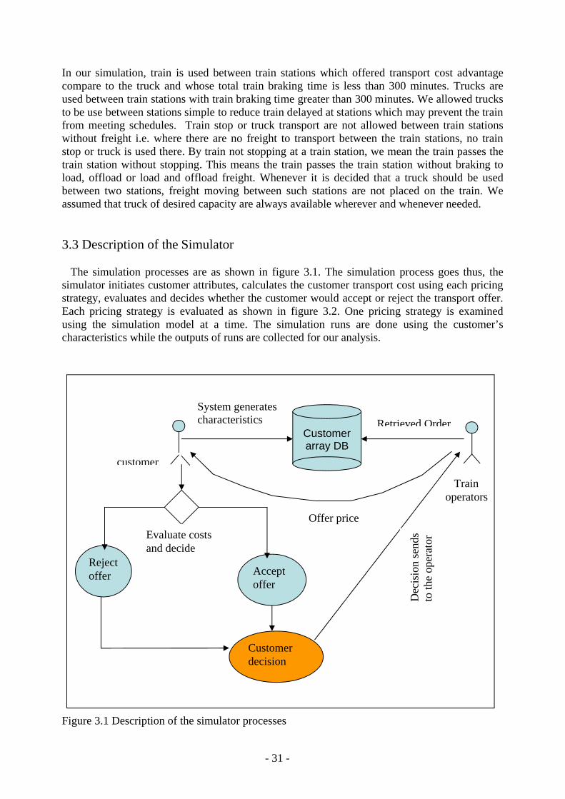
- 31 -

In our simulation, train is used between train stations which offered transport cost advantage compare to the truck and whose total train braking time is less than 300 minutes. Trucks are used between train stations with train braking time greater than 300 minutes. We allowed trucks to be use between stations simple to reduce train delayed at stations which may prevent the train from meeting schedules. Train stop or truck transport are not allowed between train stations without freight i.e. where there are no freight to transport between the train stations, no train stop or truck is used there. By train not stopping at a train station, we mean the train passes the train station without stopping. This means the train passes the train station without braking to load, offload or load and offload freight. Whenever it is decided that a truck should be used between two stations, freight moving between such stations are not placed on the train. We assumed that truck of desired capacity are always available wherever and whenever needed.

3.3 Description of the Simulator

The simulation processes are as shown in figure 3.1. The simulation process goes thus, the simulator initiates customer attributes, calculates the customer transport cost using each pricing strategy, evaluates and decides whether the customer would accept or reject the transport offer. Each pricing strategy is evaluated as shown in figure 3.2. One pricing strategy is examined using the simulation model at a time. The simulation runs are done using the customer’s characteristics while the outputs of runs are collected for our analysis.

Figure 3.1 Description of the simulator processes

Accept offer

Customer array DB

Reject offer

Train operators

Retrieved Order

System generates characteristics and stored

Offer price

Evaluate costs and decide

customer

Customer decision

Dec

isio

n se

nds

to th

e op

erat

or

oper

ator

s

- 32 -

Characteristics Outputs (Customer parameters) response

Figure 3.2 Strategy incorporated into the model to examine it performance using customer’s characteristics

During the simulation, we assumed there are customers who want to transport freight from one place to another. Each simulation process begins when the simulator received a default customer characteristic (customer 0 in our simulation model). The default customer simply tells the simulator to set states to their initial. This prepares the simulator for receiving customers. It sets all events in the simulator to the initial states. The current available train capacities of the train stations are set to full trainload. The departure days and transport schedule days are set to their respective days. The station loading time, offloading time, load, offload, are set to zero. All customer characteristics are initialised (System generates characteristics) and stored in a multiple dimensional array.

Starting with the first customer (customer 1) on the array, the simulator retrieves the customer characteristics. It retrieves the customer freight origin, destination, load, start and end train station, departure day and transport order request placement date from the customer array database. It uses the customer start train station, end train stations and load to evaluate, as in equation 1.3.0, if his load can be accommodated between his preferred train stations. If the load cannot be accommodated, the simulator tries possible start train stations, end train stations and departure days as described on searching alternate start and end train stations and generating departure days in section 3.2.3. If no train stations or day is found that can accommodate the customer load, the system immediately exits the customer by rejected his retrieved characteristics and moves to the next customer on the array queue. When there are train stations that can accommodate the customer freight, the simulator proceeds to calculate the direct cost using equation 1.5, the rail price (price to offer the customer for transporting his load from the start train station to the end train station) which depends on the strategy being used (using equation 1.6 if using constant pricing strategy and either case1, case2 or case3 for dynamic pricing strategy depending on the situation). The system, then proceeds to calculate the cost of transporting the freight from origin to the destination using train on part of the journey. This is the cost of transporting the freight from the freight origin to the start train station using the connection truck plus the cost of transporting the freight from start train station to the end train station using train plus the cost of transporting the freight from end train station to the freight destination using connection truck. The cost of moving the freight from origin to the start train station and from end train station to the freight destination are determined by equation 1.5 while the cost of moving the freight from start train station to the end train station depending on the strategy being considered. It compares the direct all-road cost and the combined rail-truck cost of transporting the customer freight from freight origin to freight destination (in figure 3.1 can be seen as (Offer price) to the customer who compared the costs).

If the cost of transporting the freight through the combined rail-truck system is less than the direct cost, the system assumed the customer has accepted the transport offer (Evaluate costs and decide) else, the system check alternate train stations and days between and from the customer preferred train stations and departure day that can accommodate the customer freight as in section 3.2.3. It recalculates the combined rail-train cost if alternate train stations or

Simulation model which runs the characteristics with the strategy

- 33 -

departure days are found that can accommodate the customer load and compares the new (reoffered price to the customer to reevaluate the transport options) cost with the direct all-road cost. If no train stations or departure day is found that can accommodate customer freight with the combined rail-truck cost less than the direct transport cost, the customer is considered to have refused the price offer. In general the customer sends his decision back to the train operators (Decision sends to the train) but in the model, the system rejected the customer’s retrieved characteristics.

When a customer accepts the transport offered, the system updates the available train capacity, train station load, offload, loading time, offloading time, train stopping time and income (revenue generated). The available train capacity at each train station within the customer travel sub leg except his end train stations are updated as in equations 1.3.2, 1.3.3 and 1.3.4. The train station corresponding to the customer start train station load and offload are updated as in equations 1.1.0 and 1.1.1. His start train station loading and offloading time are updated as in equations 1.2.1 and 1.2.2 while the train station corresponding to the customer end train station load and offload are updated as in 1.1.2 and 1.1.3. His end train station loading and offloading time are updated as in equations 1.2.3 and 1.2.4. The total train braking time at the start and end train stations are updated as in equation 1.2.5. In other to keep track of the revenues that are accruing, the total income that accrues when a customer accepts and pays for the transport demand is also updated. This is by adding to the revenue of his departure day an amount equals to the expected train price the customer will pay for transporting his freight from his start to end train station. The price the customer pays is calculated from either 1.6 or any of case1 case2, case3, depending on the strategy.

After the updating processes have finished, the system checks if the entire customers have been examined. If there are still customer(s) on the queue, it retrieves the next customer characteristics on the queue. It treats the customer in the same manner or performs similar processes on the customer. Customers are examined in the order in which their data are stored in the array i.e. from customer 1 to customer 100. When the entire customers have been examined, the simulator proceeds to check train stations where a train or truck should be used.

When all the customers have been examined, the simulator starts from the first departure day to the last departure day, from the first train station to the last but one train station, taking two train stations at a time, first, assembled the load moving between the different stations and determined if a truck or a train should be use between the two train station. For each pair, it evaluates the cost of using a truck, train and the train stopping time between the train stations. If the truck cost is less than train cost or if the train stopping time is greater than 300 minutes, truck is assigned between the stations else a train is assigned, provided there are load moving between the stations. The truck cost between the stations is calculated using equation 1.5 while the train cost is calculated as in section 3.2.3. To measure the profitability of the combined train-truck system, the simulator keeps track of the revenue that accrued due the combined service between the train stations. At the start of the simulation, the combined transport cost was zero. When a truck or a train is assigned between any two train stations, a cost equals the corresponding cost of the mode is added to the cost of the combined service i.e. the cost of the combined services increased by an equivalent amount. When all the train stations of the day have been examined, the combined cost is subtracted from the revenue that accrued during the loading process (when freight was being received from the customers). The difference between these costs became the profitable obtained due to the combined transport services. The entire simulation processes are as shown in figure 3.3. A simulation terminates when customer 1 to customer 100 has been examined i.e. a simulation is a complete examination of customer 1 to customer 100.

- 34 -

Customer Characteristics,generated randomly bythe simulator If day >generated departure +3

No Yes If minimum available train capacity-load>=0

No Yes Yes

If next station > generated station + 3 If cost through train < Direct cost No Yes

Total stopping time at stations

Select Start/end train station

Calculate direct cost

Select next train stations

Calculate train price between stations

Calculate transport cost through train

start

Initialization

Load Freight origin Freight Destination

Customer call

Update train status

Update station status

Update stations

load/offloading time

Update stations stopping time

Select next departureday

Select departure day

stop

Update Amount for the day

- 35 -

Has all customers been examined? No Yes

If train cost < truck cost and Total train stopping time between train stations <=300 No Yes

No if next = last train station

Yes

No if fixed train station = last train station.

Yes

Calculate train cost between the train stations

Calculate truck cost between the train stations

Cost between the train station =truck cost

Cost between train station =train cost

Update combined transport cost

Next station = next station +1

Select First station = fixed train station +1

Select next station = train station after first train station

Select First station= first train station

Select day = first departure day

- 36 -

Yes

No If Day > last departure day

Yes

Figure 3.3 The Entire Simulation Processes.

Profit = Amount- combined transport cost

stop

Selected Day =selected day +1

- 37 -

4 Simulation Result and Analysis

This section presents our data sources, verification, validation and the analysis of our result.

4.1 Data sources

Figure 4.1 reports the total revenue generated at different train cost per cargo-distance (Cld2). It shows the transition from using only direct truck transport to the use of rail and truck transport. The figure was arrived at by holding the truck cost per unit cargo-distance (Cld), obtained from literature, fixed while the train cost per cargo-distance were tuned to the different price levels found on the horizontal axis. The tuning was conducted with our base test scenario, the constant pricing strategy. Similar tuning was conducted using the dynamic pricing strategy with a similar graphical structure obtained. From the figure, direct all-road truck transport is competitive at and above the train charge of 1.4 SEK per ton-mile. At and above the train cost per cargo-distance of 1.4 SEK, the train operators generate no revenue. Combined rail-train transport provides the freight transporters no transport cost advantage. The direct cost of transporting freight from freight locations to the destinations provides advantage to the freight transporters than the cost of transporting the freight using the combined rail-truck system. Rail-truck transport becomes competitive at train charge per ton-mile which are less than or equal to 1 SEK. The rail operators in the combined rail-truck transport system generate maximum revenue at the train charge rate of 0.5 SEK per ton-mile. The competitive points for the truck and rail transport mode are influence by their threshold costs. In our model, we have sprayed the threshold costs over the entire customer since we perceived it would give less cost per unit ton transport to the freight transporters. The truck cost per cargo-distance was obtained directly from the literature [57] and it value as reported by the literature is 1.4 SEK per ton-mile.

We are considering in our model the train cost per unit cargo-distance (Cld2) of 0.5 SEK since it is the charge rate where the highest revenue is generated. Our choice of 0.5 SEK per ton-mile is from the perspective of the train operators who are seeking a cost rate which will enable maximum revenue to be generated even though maximum train utilisation may not be achieved at such rate.

- 38 -

0

5000

10000

15000

20000

25000

30000

35000

40000

45000

50000

0,0

0 k

r

0,0

5 k

r

0,1

0 k

r

0,1

5 k

r

0,1

6 k

r

0,1

7 k

r

0,2

0 k

r

0,4

0 k

r

0,4

5 k

r

0,4

9 k

r

0,5

0 k

r

0,5

1 k

r

0,5

5 k

r

0,6

0 k

r

0,7

0 k

r

0,8

0 k

r

1,0

0 k

r

1,4

0 k

r

Train price per Cargo-distance

Re

ve

nu

e G

en

era

ted

Figure 4.1 Revenue generated at different train cost per Cargo-distance for the constant pricing strategy

The other variable values used in our simulation are known (obtain from literature), determined or calculated by the model. Details of the variables, sources and how the values were obtained are presented in the table 4.1. The distances are calculated by the system. The load values are supplied by the freight transporters i.e. the system retrieved from the data stored in their array database. Some values were derived or confirmed with corresponding values retrieved from [51]

Variable Value (in SEK)

Source(s) How the value was obtained

F1 74.3 [41] [48] [49] [57] Drayage costBy taking the average of minimum and maximum range values and dividing the result by 15 to obtain cost per ton and converting the result from dollar to Swedish Krona. The result was compared with value from [49]

C 8.8 [48] By taking the average of minimum and maximum range values and converting the result from dollar to Swedish Krona

Cld 1.4 [57] Value retrieved directly and converted

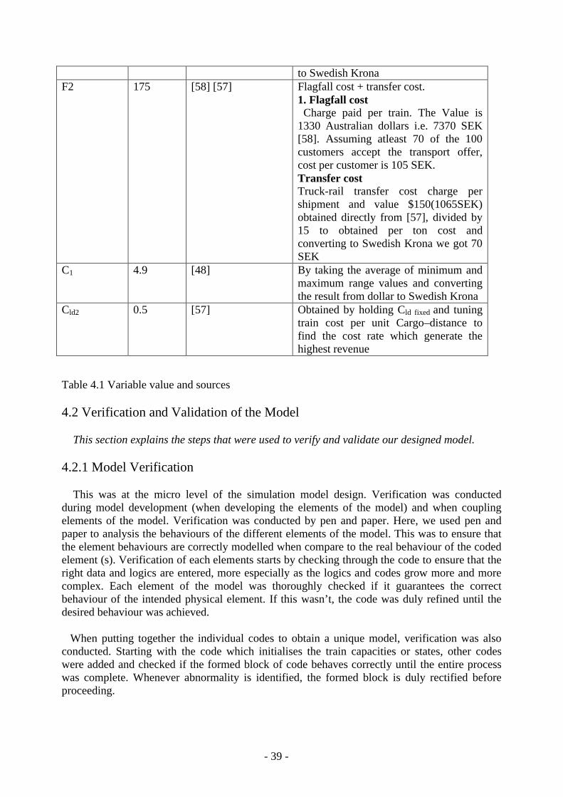
- 39 -

to Swedish Krona F2 175 [58] [57] Flagfall cost + transfer cost.

1. Flagfall cost Charge paid per train. The Value is 1330 Australian dollars i.e. 7370 SEK [58]. Assuming atleast 70 of the 100 customers accept the transport offer, cost per customer is 105 SEK.Transfer costTruck-rail transfer cost charge per shipment and value $150(1065SEK) obtained directly from [57], divided by 15 to obtained per ton cost and converting to Swedish Krona we got 70 SEK

C1 4.9 [48] By taking the average of minimum and maximum range values and converting the result from dollar to Swedish Krona

Cld2 0.5 [57] Obtained by holding Cld fixed and tuning train cost per unit Cargo–distance to find the cost rate which generate the highest revenue

Table 4.1 Variable value and sources

4.2 Verification and Validation of the Model

This section explains the steps that were used to verify and validate our designed model.

4.2.1 Model Verification

This was at the micro level of the simulation model design. Verification was conducted during model development (when developing the elements of the model) and when coupling elements of the model. Verification was conducted by pen and paper. Here, we used pen and paper to analysis the behaviours of the different elements of the model. This was to ensure that the element behaviours are correctly modelled when compare to the real behaviour of the coded element (s). Verification of each elements starts by checking through the code to ensure that the right data and logics are entered, more especially as the logics and codes grow more and more complex. Each element of the model was thoroughly checked if it guarantees the correct behaviour of the intended physical element. If this wasn’t, the code was duly refined until the desired behaviour was achieved.

When putting together the individual codes to obtain a unique model, verification was also conducted. Starting with the code which initialises the train capacities or states, other codes were added and checked if the formed block of code behaves correctly until the entire process was complete. Whenever abnormality is identified, the formed block is duly rectified before proceeding.

- 40 -

Finally, when the unique model was built, verification was also conducted using pen and paper. The check conducted at this level was on the output reports of simulation run. We checked why certain behaviours of the model were as the appeared and that the behaviours were the expectation of the model. Verification of the model elements were also through testing, observing and analysing the output reports of different sub simulation model runs and using graphical reports of samples from different simulation run outputs, sometimes with slight adjustment in the input. Comparing trends from these graphs enable us to determine if the elements are duly modelled.

4.2.2 Model Validation

This is verification at the macro level of the model. The main validation tasks was to verify that the current available train capacity of the train stations and the minimum train capacity within the travel sub legs are accurately updated and identified and to check if the difference between the customer load and the available train space is greater than or equal to zero. Cost relationships and the reliability of identifying the right combination of cost parameters and design options were also vital tasks to validate. Also among the main validation task was the ability of the model to select the right price equation during dynamic pricing. We used continuous train capacity updating and storing processes and the displaying of result to check if the current available train spaces are accurately updated. The updating and storing processes were done immediately after each customer accepts the transport offer. Each time the capacities are updated, the results are stored in an array. The result were displayed on the screen from where we analysis and do any necessary refinement on the model whenever needed. We used search techniques which always find the true minimum available train capacity among the selected options within travel sub legs. This algorithm accurately identify the minimum available train capacity within travel sub legs but limited because the search time and space became very large when the number of options to evaluate along the travel leg become too large for most real-world problems. To ensure that the difference between the current minimum train spaces within the travel sub legs are never less than zero, we ensured that it is the first thing the system checks when each customer appears. Simulation runs of the designed model with displayed of the minimum available train space within the customer travel sub leg, customer load and the different between the minimum available train space and customer load were conducted and analysed. Identified errors were duly corrected.

The following methods were also used in the model validation process:

1) Face validation. Here, time was spent watching the model as it runs. During this time, we checked why certain observed behaviours from the simulation run happen as observed. We analysed why customers are rejected or accepted at certain train stations, why customers are accepted at train stations difference from their closest train stations (whether their rejection at their closest train stations are because of price or their freight could not be accommodated), why the customers are rejected during a departure days and accepted during other departure days (whether their rejection were because their load could not be accommodated or because of price and if because of price, we checked whether their acceptance at other train station are because their transport order replacement day has became farther from their new departure day). Some times during this period, we forced certain conditions to occur so that we can study the model behaviour under specific circumstance. We some times conduct simulation run of our model and present the range of inputs and reports obtained to other (friends) who have knowledge in simulation and obtained feedback on the accuracy of the model and its ability to meet the

- 41 -

objective of the project. We at times discuss our project objectives and the types of result we have obtained from the model with others. During these discussions, we obtained differentviews on how the model will behaviours, the type of results that should be expected, how the parameters should be tuned to get better results and conditions under which abnormalities should be expected. Base on the knowledge gained from these discussions, we modified and tried different options to see how the model will behave. This enables us to learn and identify abnormal behaviours of the model and duly rectified necessary errors.

2) Comparing the Model with the Real System. Here, we compared the model performance with the real train-truck system. Since data from real system was not in existence, the comparison was done by expectations and intuition, which were main experience and knowledge gained from slightly similar existing system and literatures. The comparison was through changing the model input data, running the simulation and collecting the results of the different changes. Relationships between the inputs and outputs of these results were mapped and compared with data collected from literatures. An example was the case where we considered the price per unit cargo-distance for the train to be the same as those of the truck. In real system, since the distance which would be covered during the combined rail-truck system is greater than the direct distance from origin to the destination and since the threshold cost incurred by the combined transport mode is greater than that of direct all-road transport, it was expected that the cost of direct all-road transport would always be favour compare to the cost the combined rail-truck transport for all customers. Simulation runs were conducted for this case and the results obtained were compared with our expected known real behaviour. It was observed that 20% of the customers were accepted for the combined rail-truck service. This was an abnormal expectation from the model. This was duly corrected.

3) Objective Validation. One means of validating our model was by using the model objectives. Here, we check if the model meets its objectives. When our model was observed to behave correctly, we check if the model meets the requirements of our project objectives. These include check on the effects of inaccuracies in those data that have been estimated. This was through sensitivity analysis of our model. Starting with a significant change on the values of the estimated parameters so that we can obtain an initial feeling for the model sensitivity. Smaller incremental changes were made and the result recorded. From the sensitivity analysis, the validity of the model with respect to slight change in estimated data were predicted. The main estimated variable considers during our sensitivity analysis was the train cost per cargo-distance (Cld2). It was found that the model is very sensitive to change in the input data about our selected value (0.5 SEK per tonne-mile). It is worth pointing that the sensitivity analysis was performed on more than one set of data and such, the interaction of these data were investigated in detail before a conclusion was reached. This was through changing the data independently and together in order to observe the effects of the individual data as well as their combined effects on the simulation results. The behaviour of the model during the sensitivity analysis is shown in figure 6.1. It is also worth noting that validation of the model as well as the sensitivity analysis of the model was conducted with our base scenario (constant pricing strategy).

4.2.3 Sensitivity analysis

Figure 4.2 presents the average train space sensitivity of our model with respect to the train cost per cargo-distance (Cld2) during the constant pricing strategy. The graph shows high sensitivity about our estimated cost value (0.5 SEK per unit ton-mile) where slight change in

- 42 -

any direction (toward the right or left) is remarkably portrayed. From the graph, the train space utilisation increases with change always from the 0.5 SEK per ton. The train space utilisation increase with changes toward the left of 0.5 and decreases with changes toward the right of 0.5.

0

500

1000

1500

2000

2500

3000

3500

4000

4500

50000

,00

0,0

5

0,1

0

0,1

5

0,1

6

0,1

7

0,2

0

0,4

0

0,4

5

0,4

9

0,5

0

0,5

1

0,5

5

0,6

0

0,7

0

0,8

0

1,0

0

1,4

0

Train price per Cargo-distance

Tra

in S

pa

ce

Us

ed

Figure 4.2 Average train space sensitivity with respect to changes in the train cost per unit load-distance ((Cld2))

4.3 Results and Analysis

This section presents our analysis of the simulation results.

4.3.1 Capacity and revenue analysis

100 simulation runs were conducted using each pricing strategy (dynamic or constant pricing approach). A simulation represents a situation where customer 1 to customer 100 has been examined. Table 4.2 and 4.3 report the average quantity of freight which were transported between the train stations during 100 simulations. Table 4.2 reports the quantity of freight which were transported between the train stations during the dynamic pricing strategy while Table 4.3 reports the quantity of freights which were transported between the train stations during the constant pricing strategy. In Table 4.2 and 4.3, the Station No represents the train station, Day1, Day 2, Day3, Day4, Day5 represent the departure days. The figures are recorded in-between the train station numbers because they represent the quantity of freight that aretransported between the two train stations during 100 simulations. For example in table 4.2, a

- 43 -

total of 27247 tonnes of freights were transported by the train from train station 1 to station 2 in departure day1, 57248 tonnes of freights were transported by the train from train station 6 to train station 7 in departure day 3 etc, during 100 simulation. These amounts are the total quantity of freights that were on the train between the two train stations. Total load represents the quantity of freights that were transported by the train between the two train stations during the five departure days and during the 100 simulations. Average represents the mean quantity of freights that were transported between the two train stations during 100 simulations and fivedeparture days. Percentage represents the daily percentage of the train space used between the two train stations. The mean daily percentage of the train space used between the train stations during dynamic pricing strategy is 41.47 %, while that of the constant pricing strategy is 40.28 %. 1.19 % of interstation train spaces are used during the dynamic pricing strategy than the constant pricing strategy. Divergence from the mean represents the difference between the daily percentage of the train space used between the train stations and the mean daily percentage of the train space used. Positive Sign indicates values above the mean daily percentage train space used while negative sign indicates values below the mean daily percentage train space used. For detail information on the quantity of freights that were moving from one train station to another during the 100 simulations and during each departure day for both the dynamic and constant pricing strategies, see Appendix A.

Station No Day 1 Day 2 Day 3 Day 4 Day 5 Total Load Average Percentage Deviation From mean

127247 29146 26092 25923 24162 132570 265.14 26.5 -14.96

233339 38687 35909 35028 32324 175287 350.574 35.06 -6.42

334548 39634 39141 35954 33233 182510 365.02 36.50 -4.97

444166 48802 46522 46098 43162 228750 457.5 45.75 4.28

550665 55457 53430 52882 49256 261690 523.38 52.34 10.86

653886 59526 57248 57841 53431 281932 563.86 56.39 14.91

751933 57254 55933 56259 51973 273352 546.70 54.67 13.20

843592 47076 46719 44732 46276 228395 456.79 45.68 4.20

918717 20494 21060 21278 20332 101881 203.76 20.38 -21.10

10

Mean daily percentage train space used 41.47Standard Deviation from the mean 11.95

Table 4.2 Average quantity of freight transported between train stations during the dynamic pricing strategy

- 44 -

Station No Day 1 Day 2 Day 3 Day 4 Day 5 Total Load Average Percent Deviation From mean

127033 25018 25324 25704 27617 130696 261.39 26.14 -14.14

235514 34980 34576 35772 36828 177670 355.34 35.53 -4.74

3 036856 35817 36212 37086 37839 183810 367.62 36.76 -3.52

446283 45232 46023 47119 46930 231587 463.17 46.32 6.04

552734 49721 51159 52106 52442 258162 516.32 51.63 11.36

655888 52809 55073 54959 51113 269842 539.68 53.97 13.69

753791 51202 53201 52495 49373 260062 520.12 52.01 11.74

843438 41227 43349 43068 38877 209959 419.92 41.99 1.72

918364 19681 20203 18611 13832 90691 181.38 18.14 -22.14

10

Mean daily percentage train space used 40.28Standard Deviation from the mean 11.64

Table 4.3 Average quantity of freight transported between train stations during constant pricing strategy.

Figure 4.3 presents the percentage train space used between the train stations during the dynamic and constant pricing strategy i.e. average daily percentage of the train capacity used between the train stations. From the figure, maximum and minimum train capacity usage, during the dynamic pricing strategy, was achieved between train station 6 and train station 7 and train station 9 and train station 10 where 56.39% and 20.38 % of the train capacity were used. During the constant pricing strategy, the maximum and minimum train capacity are used between train station 6 and train station 7 and train station 9 and train station 10 when 53.97 % and 18.14 % of the train capacity were used. The maximum train space used during dynamic pricing strategy is greater than that of the constant pricing strategy. The mean daily percentage train capacity used during the dynamic pricing strategy is greater than that constant pricing strategy (i.e. 41.47>40.28). The minimum daily percentage train space used during the dynamic pricing strategy is high than that of the constant pricing strategy. This shows that more train space are used during the dynamic pricing strategy than the constant pricing strategy. From the mean daily percentage of the train space used, an average of 1.19 % of the train space are achieved during dynamic pricing over constant pricing strategy between every two closer train stations i.e. each time the train moved from one train station to the next train station, the operators achieved an increase of 1.19 % in the train capacity used during dynamic pricing than the constant pricing. This shows that the dynamic pricing strategy gives an advantage of 1.19 % in interstation train space usage over the constant pricing. This percentage gives an average of 11.9 (1.19*1000/100) tonnes in interstation space used or approximately 12 tons of freights are accepted and transported between every two closest train

- 45 -

stations. This means between every two nearest train stations, there is an increase of 12 tons in the quantity of freight accepted from customers during dynamic pricing compare to constant pricing. Summing this for the 10 train stations, we got an average increase of 107.1 (11.9*9) in the train space used during each departure day during the dynamic pricing strategy than the constant pricing strategy. The revenue which accrued to the train operators due to this quantity of freight is approximately 502.73 SEK per departure day

The minimum and maximum train spaces used during the dynamic pricing are greater than those of the constant pricing. This is an indication that high train capacities are used during dynamic pricing strategy than the constant pricing strategy.

A closed examination of Figure 4.3 shows that the percentage train capacity use between the train stations increases steady from train station 1 until it reaches a maximum value between train stations 5 and train station 6, from which it starts to decrease. This indicates that the accepted freights are distributed among the different train stations. Freights acceptance is spread through the entire train stations. This is because of the possibility of accommodating customer freights at other train station. This is more pronounced in the dynamics pricing strategy than the constant pricing strategy as prices within overcrowded travelled sub legs causes train customers to consider less crowded travelled sub legs. This is the reason why the train spaces used are almost high between all train stations during the dynamic pricing strategy than the constant pricing strategy. Since prices at crowded train station caused customer to consider less crowded train stations where there are enough available train space, more train space are used at many train stations during the dynamic pricing strategy than the constant pricing strategy. This means, during dynamic pricing strategy, the possibilities of generating alternate train stations and departure days for the customers are more pronounced than in constant pricing strategy, since prices are different within different train stations and departure days. This explained why more customers are accepted and more train capacity are used during dynamic pricing strategy than constant pricing strategy, as there are likelihood that other train stations or departure days can accommodate the customer freight at prices lower than the direct cost of all-road transport using truck. Prices at travel sub legs with high transport demand caused customer to consider alternate train stations or travelled sub legs. This caused the percentage train capacity used not to grow extremely higher at specific travelled sub leg but to be distributed among the entire train stations. Reason being that when one point along the travel sub leg has a high freight transport demand, the train price at such point(s) scared many customers from considering such points between their start and end train stations. Train prices at travel sub leg before or after these points caused customers to consider end train stations before these points or to consider placing transport order between train stations that do not contain the points.

Another indication of the high percentage train capacity used between the train stations and the distribution of the accepted freight among the train stations during the dynamic pricing strategy can be seen from the high mean daily percentage of the train space used and the high standard deviation of the mean daily train space used between the train stations during the dynamic pricing strategy than the constant pricing strategy. High standard deviation (with mostly positive deviation from the mean) about a high mean, during the dynamic pricing strategy than constant pricing strategy is due to the high mean daily percentage train capacity used during the dynamic pricing strategy. The mean daily percentage of the train capacity used between train stations during the constant pricing strategy is clustered to the small mean percentage of the train space. Reason why the standard deviation from the mean is small compare to that of the dynamic pricing strategy. The mean daily percentage of the train capacity used during dynamic pricing is high between train stations than the constant pricing.

- 46 -

The low values of the percentage train space used between the train stations during the constant pricing strategy than the dynamic pricing strategy are due to the non-variation in prices among the travel sub legs. Customer are not discourage from considering crowed travel sub-leg and as such considering alternate train stations by the customer is less effective compare to the dynamic pricing.

0

10

20

30

40

50

60

1 2 3 4 5 6 7 8 9 10

Train stations

Pe

rce

nta

ge

tra

in s

pa

ce

us

ed

Percentage train space used during dynamic pricing strategy

Percentage train space used during constant pricing strategy

Figure 4.3 Average percentage train capacity used between train stations during dynamic and constant pricing strategy

During the Constant pricing strategy, prices at overcrowded train stations or travel sub legs do not discourage customers from considering such train stations as in dynamic pricing. This is because there are no defined means which can encourage customers to consider other start and end train stations when there is a high transport demand along a travel sub-leg rather than that his freight can not be accommodated or cost advantage is not achieved along such travel sub legs. When customer freights are not accepted within her travel sub-leg, the probability of the customer accepting the transport offer along other travel sub leg is very low compare to that of the dynamic pricing strategy. The customers are placed in situation where they think very little about considering other train stations. They are limited to comparing the price offered by the operators at their closest train stations (closest train station to their freight destination and

- 47 -

freight origin), when their freight can be accommodated on the train, and checking if it gives transport cost advantage over direct transport. If not, the customer has high probability of rejecting the transport offer since prices which would be obtained at other train stations which he may consider are calculated the same. Even though the alternate train stations and departure days are not pronounced during constant pricing, it positive effect on the constant pricing strategy is not neglected. Steady raising and falling of the percentage train space between train stations are due to the provision of alternate train stations and departure days to the customers. This provision allowed some customers whose freights cannot be accommodated within some travel sub-leg to be accommodated at other travel sub-leg during the same departure day or other departure days. Lack of a defined means of discouraging customer from considering a travel sub-leg is a cause of less revenue generated and less freight quantity accepted during constant pricing than the dynamic pricing.

Table 4.4 and 4.5 show the number of customers that accepted transport offer (No), the total freights accepted from the customers (Load), total revenue generated by the train operators (Train Price), the total connection cost incurred by freight transporters in transporting their freights to the train stations and always from the train stations (connection cost), total cost spent by the customers when using rail-truck transport (Total cost through train), the direct cost of transporting the freights from origins to destinations (Direct cost), total distances through which the freight were transported through the train (train distance) and connection truck (connection distance) , the direct distance through which the freight would have moved (direct distance) and the conditions under which the values were obtained during the dynamic and constant pricing strategy.

On an average, more revenue was generated during the dynamic pricing strategy than the constant pricing strategy. An average of 42109.58 SEK was generated as revenue per simulation during the constant pricing strategy while 44623.25 SEK was generated during the dynamic pricing strategy. Dynamic pricing strategy generates 2513.67 SEK as revenue per simulation than constant pricing.

From Table 4.4, during the dynamic pricing strategy, an average of 41.1 % of the customers examined with an average load of 2876.9 tonnes accepted the transport offer when the closest train station to their freight’s locations and destinations were considered, 3.41 % of the customers examined with an average load of 179.27 tonnes accepted the transport offer when their start train stations were changed, 0.74 % of the customers examined with an average load of 41.72 tonnes accepted the transport offer when their end train stations were changed, 0.09 % of the customers with an average load of 7.3 tonnes accepted the transport offer when both their start and end train stations were altered, 0.17 % of the customers with an average freight of 10.6 tonnes accepted the transport offer when their departure days were altered and 54.29 % of the customers examined with an average load of 2880.18 tonnes denied the offer. Dynamic strategy with the provision of alternate train stations to freight customers gives an average increase of 4.41% in the no of customers who accepted the transport offer compare to dynamic pricing without the provision of alternate train stations to the customers. This percentage correspond to an average increase of 238.9 tonnes in the volume of freight transported, 3794.01 SEK in the revenue generated, a reduction of 150.15 SEK (direct cost –(connection cost + train price) in the transporters’ cost (there is a reduction of 150.15 SEK in the transport cost that these freight’s owners could have paid if there were to transport those quantity of freights directly using all-road truck transport).

From Table 4.5, of the 100 customers examined during a simulation, 39.9 % of the customers with an average load of 2629.65 tonnes accepted the transport offer when the closest

- 48 -

train station to their freight locations and destinations were considered, 3.52 % of the customers with an average load of 199.38 tonnes accepted the transport offer when their start train stations were changed, 0.66 % of the customers with an average load of 38.58 tonnes accepted the transport offer when their end train stations were altered, 0.1% of the customers with an average load of 8 tonnes accepted the transport offer when both their start and end train stations were altered, 0.11 % of the customers with an average load of 35.18 tonnes accepted the transport offer when their departure days were altered and 55.7 % of the customers with average load of 3083.8 tonnes denied the transport offer. This strategy gives an average of 4.39 % in the no of customers who accepted the transport offer during constant pricing with the provision of alternative train stations compare to constant pricing without the provision of alternative train stations to the customers. This percentage produced an average increase of 247.73 tonnes in the volume of freights transported, 2882.84 SEK in the revenue generated, a reduction of 194.05 SEK (direct cost – (connection cost + train price)) in the transporters’ cost (there is a reduction of 194.05 SEK in the transport cost that these freight owners could have paid if there were to transport these quantities of freights directly using all-road truck transport).

Black colour – value obtained during the 100 simulationsRed colour - average of 100 simulations

Table 4.4 Dynamic pricing of freight with alternative train stations provision to freight transporters

CustomerAccepted with NO Load Train Price

ConnectionCost

Total costThrough Train Direct Cost

Train Distance

Connection Distance

Total Distance

Direct Distance

4110 287690 4082924.36 3704777.38 7787701.7 9464833.29 95005.27 29986.65 119991.991648.73

Chosen TrainStation 41.1 2876.9 40829.24 37047.77 77877.02 94648.33 950.053 299.87 1199.92 916.49

341 17927 316684.44 400572.26 717256.7 727531.35 3903.82 5248.42 9152.24 7285.86Change in StartStation 3.41 179.27 3166.84 4005.72 7172.57 7275.31 39.04 52.48 91.52 72.86

74 4172 41623.44 73038,95 114662,39 115400.94 904.68 689.25 1593.93 1277.510.74 41.72 416.23 730.39 1146.62 1154.01 9.05 6.89 15.94 12.78

Change in EndStation

9 730 8727.39 15430.8 24158.19 26607.48 143.43 115.89 259.32 212.99Change in BothStart/end Station 0.09 7.3 87.27 154.31 241.58 266.08 1.43 1.16 2.59 2.13

17 1061 12365.29 18049.2 30414.49 31967.23 261.87 164.18 426.05 327.060.17 10.61 123.65 180.49 304.15 319.67 2.62 1.64 4.26 3.27

Change inDeparture Day

5449 288018 2938952.57 8240507.05 11179460 9175524.19 63076.05 84710 147786.1102509.2Denied

Offer 54.29 2880.18 29389.53 82405.07 111794.6 91755.24 630.76 847.1 1477.86 1025.09

Total Revenue generated 4462324.93

44623.25

- 49 -

CustomerAccepted with NO Load Train Price

ConnectionCost

Total costThrough Train Direct Cost

Train Distance

Connection Distance

Total Distance

Direct Distance

3988 262969 3982213.67 3594052.8 7576266.4 9233109.89 85003.04 32186.5 117189.5 89443,639.9 2629.69 39822.14 35940.53 75762.66 92331.10 850.03 321.87 1171.90 894.44

Chosen TrainStation

352 19338 230139.88 436459 666598.88 678473.94 5473.88 4139.15 9613.03 7612,733.52 193.38 2301.40 4364.59 6665.99 6784.74 54.74 41.39 96.13 76.13

Change in StartStation

66 3858 39293.43 74303.68 113597.11 114264.57 835.41 678.16 1513.57 1206.84Change in EndStation 0.66 38.58 392.93 743.04 1135.97 1142.65 8.35 6.78 15.14 12.07

10 800 7659.13 16836.59 24495.72 27260.58 183.76 229.29 413.05 316.950.1 8 76.59 168.37 244.96 272.61 1.84 2.29 4.13 3.17

Change in BothStart/end Station

11 777 11192.97 12098.56 23291.53 27389.84 238.58 146.53 385.11 253.520.11 7.77 111.93 120.99 232.92 273.90 2.39 1.47 3.85 2.54

Change inDeparture Day

5573 308380 2999558.97 8500222.9 11499782 9412602.19 63882.59 86982.98 150865.6 04443.9Denied Offer 55.7 3083.8 29995.59 85002.23 114997.82 9412602 638.83 869.83 1508.66 1044.44

4210957.82Total Revenue generated 42109.58Black colour – value obtained during the 100 simulationsRed colour - average of 100 simulations

Table 4.5 Constant pricing of freight with alternative train stations provision to freight transporters

4.3.2 Comparing Dynamic and constant pricing Strategies

Table 4.6 presents an abstraction of figure 4.7 and 4.8. The calculations are on per simulation values of 100 simulations conducted using dynamic and constant strategies. From the figure, an average of 45.71 % and 54.29 % of the customers accepted and rejected the transport offer during the dynamic pricing strategy while 44.27 % and 55.73 % of the customers accepted and rejected the transport offer during the constant pricing strategy. There is an average of 1.44 % (45.71- 44.27) in the percentage of customer who accepted the transport offer during dynamic pricing over constant pricing. The percentage of customer who rejected the transport offer, during constant pricing strategy is greater than those who rejected the offer during dynamic pricing strategy. The difference between those who rejected the transport offer during constant pricing over dynamic pricing is 1.44 %

- 50 -

Table 4.6 Abstraction from figure 4.7 and 4.8

Average Freight Transported: More freight were accepted and transported during the dynamic pricing strategy than the constant pricing strategy. An average of 3115.8 tonnes were accepted and transported during the dynamic pricing strategy while 2877.42 tonnes were accepted and transported during constant pricing strategy. An average of 238.38(3115.8-2877.42) tonnes were accepted and transported during the dynamic pricing strategy than the constant pricing strategy. On the other hand, more freight was rejected during the constant pricing strategy than the dynamic pricing strategy. Averages of 3083.8 tonnes were rejected during the constant pricing while an average 2880.18 tonnes were rejected during dynamic pricing. An average of 203.62 (3083.8 -2880.18) tonnes were rejected during the constant pricing than the dynamic pricing strategy.

Average Revenue Generated: This is the price paid to the train operators by the freight transporters for using train between the train stations. More revenue is generated during the dynamic pricing strategy than the constant pricing strategy. An average of 44623.25 SEK was generated during the dynamic pricing strategy while an average of 42704.99 SEK was generated during the constant pricing strategy. This shows that an average of 1918.26 SEK (44623.25-42704.99) accrued during the dynamic pricing than the constant pricing. More lost (income that the operators may have had if freight owners accepted the transport offer) was incurred because the customers rejected the transport offer during the constant pricing strategy

STRATEGY Dynamic pricing Constant Pricing

AcceptedFreight

RejectedFreight

AcceptedFreight

RejectedFreight

45.71 54.29 44.27 55.73No of customers who accepted Transport serviceFreight accepted and transported 3115.8 2880.18 2877.42 3083.8

Train Price 44623.25 29389.53 42704.99 29995.59

Connection 42118.69 82405.07 41337.51 85002,23Price

Total cost 86741.94 111794.6 84042.50 114997.8

Direct Cost 102663.40 91755.24 100804.99 94126.02

Train Distance 1002.19 630.76 917.35 638.83

Connection 362.04 847.1 373.80 869.83Distance

Total distance 1364.24 1477.86 1291.14 1508.66

Direct Distance 1007.52 1025.09 988.34 1044.44

44623.25 42109.58RevenueGenerated

- 51 -

than the dynamic pricing strategy. A lost of 606.06 (29995.59-29389.53) SEK was incurred by the operators during the constant pricing than the dynamic pricing.

Connection Cost: More cost was incurred during connection (cost of transporting the freight from freight location to start train stations and from end train station to freight destination) by the freight transporters during dynamic pricing strategy than the constant pricing strategy. A connection cost of 42118.69 SEK was incurred during dynamic pricing while 41337.51 SEK was incurred during the constant pricing. The difference between these two connection costs is 781.18 SEK. More connection cost during dynamic pricing than constant pricing is due to thefreight locations, destinations, starts and ends train stations which differ in both cases. This is also due to the large freight volume that was transported during the dynamics pricing strategy than the constant pricing strategy. This is justified by the ratio of the connection cost incurred to the load transported during the two pricing strategies. The ratio is greater during the constant pricing (14.37) than the dynamic pricing (13.52), indicating that more connection cost was incurred during dynamic pricing than constant pricing due to the large freight volume that are transported during the dynamic pricing than the constant pricing (see table 4.7).

Total cost: This is the total cost incurred during the transportation of the freight from freight origin to the freight destination. The freight transporters in the combined rail-truck services spent 86741.94 SEK during the dynamic pricing strategy in transporting the accepted freight. The direct all-road cost which these transporters could have paid if they were to use direct all-road transport in transporting these freights is 102663.40 SEK. With the combined rail-truck transport, a reduction of 15921.46 (direct cost – (connection cost+ train price)) SEK was achieved over all-road transport by the freight transporters during the dynamic pricing strategy. The total cost incurred by the freight transport when transporting the rejected freights was 91755.24 SEK (direct cost of transporting the rejected freights) while the cost that could have been incurred if combined rail-truck transport system was used is 111794.6 SEK (train price + connection cost of transporting of rejected freights) which is 20039.36 SEK greater than the direct cost, reason why direct all-road transport was preferred. The total cost incurred by the freight owners when transporting all the freights (rejected + accepted freight) that were available during dynamic pricing strategy is 178497.18 SEK. The percentage of the total cost paid to the train operators during dynamic pricing strategy is 25 % (train cost of accepted freight /total cost) while the fraction spent on truck is 75 % (connection cost of accepted freight plus direct cost of transporting rejected freight/total cost). The percentage of the cost spent on the combined transport mode is 48.6 %( connection cost plus train cost divided by total cost multiply by 100) while 51.4 % of the total cost was spent on directed all-road transport.

During constant pricing, an average of 84042.5 SEK was spent on the combined rail-truck for the transportation of the accepted freight. The direct all-road cost of transporting the accepted freight (if there were transported direct using direct all-road trucks) was 100804.99 SEK. The combined rail-truck transport offered transport cost advantage of 16762.49 SEK over direct all-road transport during constant pricing. The cost incurred in transporting the rejected freights through direct all-road was 94126.02 SEK while the expected cost that could have been incurred if there were transported through the combined rail-truck system is 114997.8 SEK, which is 20871.8 SEK greater than the direct all-road cost. The total cost spent by the freight transporters for transporting all the freights that were available during the constant pricing strategy is 178168.5 SEK. Percentage of the total cost paid to the train operators is 23.97 % while 76.03% was spent on truck (connection trucks and direct transport trucks). The percentage of the total cost paid on rail-truck system was 47.17 % (train cost of accepted freight plus connection trucks multiple by 100 /total cost) and 52.83 % was paid to direct

- 52 -

transport truck. It is observed that more percentages of the total cost were paid on rail and the combined rail-truck system during dynamic pricing than constant pricing.

Environmental Performance (distance covered): During the dynamics pricing, the average distance through which the accepted freight were hauled using the railways is 1002.19 miles, the connection distance hauled by trucks is 362.04 miles, the total distance covered when transporting the accepted freights from their origins to their destinations using the combined rail-truck system is 1364.24 miles and the direct distance that could have been covered by direct all-road trucks in transporting these freights from origin to destination is 1007.52 miles. The rail mode covered 73.46 % of the total distance covered in the combined rail-truck system for the transportation of the accepted freights while the connection trucks covered 26.54 %. In constant pricing strategy, the average distance covered by the railway in transporting the accepted freights in the combined transport mode is 917.35 miles, the connection truck s covered 373.80 miles, the total distance covered by both the connection trucks and the train is 1291.14 miles while the expected direct all-road distance that the accepted freights could have covered is 988.34 miles. The percentage of the combined distance covered on railways in transporting the accepted freights is 71.05 % while the distance covered by the connection trucks during the constant pricing strategy is 28.95 % of the total combined distance. This shows the rail covered more distance than the connection truck in both cases. But the percentage of the combined distance covered by the rail during the dynamic pricing strategy is greater than that of the constant pricing strategy.

Environmental Performance of Unaccepted Freights: The average expected distance that were to be covered using railways was 630.76 miles, the average expected connection truck distance that were to be covered was 847.1 miles, the total expected truck and train distance in the combined system was 1477.86 miles and the direct distance through which the freight were transported using direct trucks is 1025.09 miles for the dynamic pricing strategy. Those of the constant pricing strategy are 638.83 miles for the average expected rail distance, 869.83 miles for the average expected connection distance, 1508.66 miles for the total expected average combined transport system distance and 1044.44 miles for the average direct distance that was used to transport the freight. It is observed that in both strategies, direct transport gives cost advantage over the combined transport system because the freights were to be transported through long distances on connection trucks and very short distance on the train.

Environmental Analysis of the Total Freights Examined during the Strategies: The total distance covered to transport the entire freights that were examined or available during dynamic pricing is 2389.33 miles (total distance through which the accepted freights were transported plus the total distance covered by direct truck to transport the rejected freights). The proportion of the distance covered by the railway is 41.95 %( rail distance of accepted freight / total distance through which the available freight during the strategy was moved), the connection truck covered 15.15 % and the direct trucks covered 42.9 % of the total distances. The trucks (both connection trucks and trucks which transport freight directly from origin to destination) hauled 58.05 % of the total distance. The combined transport system covered 57.1 % of the total distance while the direct all-road truck covered 42.9 % of the total distance.

During the constant pricing strategy, the total distance through which the total freight that was available for the strategy was hauled through is 2335.58 miles (distance covered during the transportation of rejected freights plus the distance covered by train and truck in the transportation of freight that were accommodated on the train). The proportion of the distance covered on railway is 39.28 %, the connection trucks covered 16 %, direct transport trucks represents 44.72 % of the total distance covered by the available freight. In term of truck (the

- 53 -

connection truck and direct truck) and rail, the trucks hauled 60.72 % of the total distance while the rail hauled 39.28 %. The combined transport system covered 55.28 % of the total distance while the direct all-road truck covered 46.72 % of the total distance. It is observed that the proportion of the distance hauled on rail during the dynamic pricing strategy is greater than that of the constant pricing strategy. Also, the combined transport system covers longer distance than direct all-road truck during the dynamic pricing strategy than the constant pricing strategy.

4.4 Analysis in Term of Ratios

From Table 4.7, the gross cost per unit ton paid for the transportation of the accepted freight on rail transport mode is lower during dynamic pricing of freight than during constant pricing of freight by 0.52 Sek. The gross connection cost paid by the freight transporters for connecting the freight to and from the train stations per ton is lower during the constant pricing strategy than the dynamic pricing strategy. This implies less is paid per ton on rail-truck system by the freight transporters both on the train and connection trucks during the dynamic pricing strategy than the constant pricing strategy. This means dynamic pricing provides cost advantage to the freight transporters than constant pricing. It means the dynamic pricing strategy provide gross cost advantage to the transporters on both truck and rail transport modes.The connection cost per ton is greater during the constant pricing strategy than the dynamic pricing strategy, implying the freight transporters spend much in connection their freight during constant pricing strategy than the dynamic pricing strategy. The gross total cost per unit ton incurred in the combined rail-truck transport system is higher during the constant pricing than dynamic pricing (i.e. 35.03>32.95). This implies the dynamic pricing strategy does not only provide modal cost advantage than constant pricing but also the combined cost advantage to the transporters. Dynamic pricing strategy offered on overall less cost per unit ton transported to freight transporters than the constant pricing strategy.

For the rejected freights, the expected train cost per unit ton is higher during the dynamic pricing strategy than the constant pricing strategy. The expected connection cost per unit ton is greater during the dynamic pricing than constant pricing. The expected total cost per unit ton that could have been incurred if the combined rail-truck transport was used is higher during dynamic pricing than the constant pricing. Here, it is observed that the expected gross connection cost per ton of transporting the rejected freight is about 3 times greater than the gross rail charge (cost) per ton of transporting the rejected freight in both dynamic and constant pricing strategy. This implies freights are rejected if their connection cost per ton is greater than the train cost per ton. This shows that much amount of money was to be spent on connection truck than was to be spent on the train. This is another indication of the long distances that the freights were to spend on the connection trucks than on the train. Reason why the connection cost per ton is higher while the transport ton per mile during connection is lower than those of the dynamic pricing strategy.

- 54 -

* Values that could have got if freight were transported through combined rail-truck transport system.

Table 4.7 Cost/price per load and load per kilometre ratios

T-Test: A T-test was conducted on the revenue generated during the dynamic and constant pricing strategy. This gives a one-tail probability of 95 % while our result of the T-test conducted on the average train space utilisation between the train stations gives a one-tail probability of 76.1%. From these results, we can conclude that our hypothesis that the dynamic pricing strategy yields the best space utilisation than the constant pricing strategy is statistically significant or not by chance.

Direct Cost Versus Combined System Cost: Comparing the direct cost of transporting the freight from origin to destination with the total cost of transporting the freight through the combined rail-truck transport, the gross cost per ton of the combined rail-truck transport is less than the gross cost per ton of the direct all-road transport, for the accepted freight. This indicates that the transporters paid less cost per ton during the combined rail-truck transport than they would have paid in direct all-road transport of the freight from freight origin to freight destination. This means the combined Rail-Truck transport provides cost advantage to the freight transporters than the direct all-road transport. For the rejected freights, the cost per unit ton is higher in the combined Rail-truck transport than in the direct transport. This is the

Ratio Analysis

DYNAMIC PRICING CONSTANT PRICINGACCEPED REJECTED ACCEPED REJECTED

Train price per unit ton 14.32 10,20* 14.84 9.73*

Connection cost per unit ton 13.52 28,61* 14.37 27,56*

Total cost per unit ton 27.84 38,82* 29.226 37.29*

Direct cost per unit ton 32.95 31,86 35.03 30.52

Transported ton per mile on rail 3.11 4,57* 3.14 4.83*

Transported ton per mile on 8.61 3,40* 7. 70 3.55*

Connection truck

Transported ton per mile on 2.28 1,95* 2.23 2.04*Rail-truck

3.093 2,81 2.91 2.95Transported ton per mileDuring direct transport

Gross Revenue generated per 14.32 14.64Transported tonnes

- 55 -

reason why direct all-road transport of these freights was more advantageous than rail-truck transport system. This is the same for both the dynamic and constant pricing strategies.

Transported Ton per Distance: The transported ton per mile on the rail is greater during the dynamic pricing strategy than the constant pricing strategy. More tonnes are transported through a miles during the dynamic pricing than the constant pricing strategy. The transported ton per mile on the connection trucks is higher during the dynamic pricing than the constant pricing. This means during connection, more tons of freights are transported through every mile during dynamic pricing strategy than the constant pricing strategy. This is a reason for the achieved transport cost advantage during dynamic pricing than constant pricing. This is because freight travelled longer distances on the train and shorter distances on the connection truck during dynamic pricing strategy than the constant pricing strategy. The total transported ton per mile (gross ton per mile) in the combined Rail-Truck transport is greater during the dynamic pricing strategy than the constant pricing strategy. More freight was transported through every mile in the combined Rail-truck transport during dynamic pricing than constant pricing.

For the rejected freights, the expected transport ton per mile on the rail is greater during the constant pricing strategy than the dynamic pricing strategy. The expected transport ton per mile on the connection trucks is greater during the constant pricing strategy than the dynamic pricing strategy. The expected gross or total transport ton per mile on the combined rail-truck transport system is higher during the constant pricing strategy than the dynamic pricing strategy. This is an indication that large quantities of freights are rejected in the combined services during the constant pricing than the dynamic pricing.

Comparing the ton per direct distance with the ton per distance through the combined rail-truck transport system, the expected ton per mile during direct freight transport is greater than the ton per mile of the combined rail-truck system during the dynamic and the constant pricing strategy. This implies less tonnes are transported through every mile in the combined rail-truck transport system than are transported in the direct all-road transportation of freight from freight origin to destination. Moreover, in the combined transport system, very short distances are hauled using truck while long distances are hauled with the train. This is positively very good with respect to the environmental pollution since the trucks produced the greatest fraction of environmental hazard that come from the transport industry or since the train is environmentally friendly than the truck. This is inline with the fact that the combined rail-truck transport system is a means of reducing the quantity of freight transported per unit distance on our congested road transport network. It shows that the combined transport system act as a solution to the increasing freight volume and the transported volume through every distances on our transport infrastructure [15]. It is a means of reducing the negative impact of the transport industry on our environment.

Revenue generated: Less revenue is generated per transported ton during the dynamic pricing strategy than the constant pricing strategy. This is due to the high volume of freight that was transported during dynamic pricing than the constant pricing and the positive effect of the different pricing level used during dynamic pricing strategy.

- 56 -

5 Conclusion

Our developed model has proved suitable for examining performance strategies of an intermodal rail-truck system. The model could also be used for analysing strategies and relevant performance measure of the different transport modes. Also, since the model is built on passenger transport operation, the model can be used to examine or analysis the performance of passenger transport operations in other modes of transport.

Intermodal rail-truck freight services would become more competitive and can expand if dynamic pricing of freight with train capacity allocation is allowed. This is more effective if freight transporters are provided alternate travel sub-legs and departure days during the schedule period. The dependent of train price per ton–distance on the booking time from the departure day and the available train capacity along travel sub legs act as a means of encouraging freight transporters to consider less crowded travel sub leg during the dynamic pricing. While in the constant pricing, there are no defined parameters to scare freight transporters from considering Overcrowded travel sub legs. This is the reason why the dynamic pricing strategy is more advantageous than the constant pricing strategy. The dynamic pricing strategy proves to be encouraging to both freight train operators and the freight transporters. It provides high transport tons per mile on rail and connection trucks. It leads to an increased train space utilisation between the train stations and increase revenue generated by the operators. It provides less gross cost per transported ton to the transporters than the constant pricing strategy. From our analysis, we believed the dynamic pricing strategy gives the best performance and space utilisation in an intermodal line train system. It enables longer distance hauled on rail and shorter distance hauled on the road (connection truck) which is environmental advantageous with respect to reducing the high negative impact of road transport on our environment since rail transport is environmental friendly than the truck.

The results achieved with our model are similar to the conclusion proposed for the related problem by Woxenius [15], hence supporting the validity of our model.

- 57 -

6 Future Works

Our results and analysis show that the intermodal rail-truck transport services will expand and improve if dynamic pricing policy, used in passenger transport, is used into the system. We look forward to investigating deeply the dynamic pricing of freight in an intermodal transport chain. We wish to expand our model to handle freight transport request placement for the farthest future. We shall consider in future work situations where customers can book transport order for non-schedule periods as in other transport mode. We shall also consider expanding our model to handle situations where a customer or group of customers can hire the entire service, more than one customer can book transport order at the same time and situation where urgent transport request can be handle accurately. We shall also investigate situation where some customers may be offer relative low price within a travel sub leg when the departure day has almost approach without the train operator obtaining enough trainload within some travel sub legs while there is high transport demand at other travel sub legs.

During the study, we found that at very short distances, the combined rail-transport mode provides no transport advantages compared to direct all-road truck transport. This is because of the high threshold cost incurred by the rail transport mode compare to the truck transport model. We shall in our future work, search means or strategies for reducing the high threshold cost of the rail transport mode so as to make rail freight transport as well as the combined rail-truck freight transport services more competitive over direct road transport on short distances. We look forward to searching and incorporating into our model external transport costs like the environmental pollution cost, accident cost (insurance), congestion cost and infrastructure or track price.

- 58 -

7 ACKNOWLEDGEMENT

I wish to express sincere thanks to my supervisor Jan A Persson. for proposing the research caption, granting my request to work with him and for sharing his experience and knowledge with me on this thesis. I equally thank him for his unceasing advice and supports along the entire project.

I would also like to thanks friends whom with me have made this thesis what it now stands to be. To them, I say i thank you all for your support.

Many thanks also go to my family for the encouragement, financial and moral supports they have been giving me during my entire master study in Sweden.

- 59 -

8 References

“If I have seen further [than certain other men] it is by standing upon the shoulders of giants.” ---- Isaac Newton

[1] Joseph A Montagna,” The Industrial Revolution”, Contents of Curriculum Unit 81.02.06, the Yale-New Haven Teachers Institute, 2006.

[2] Garcia Isabel and Gil Gutierrez, “A simulation model for strategic planning in rail freight transport systems”, Institute of transportation engineer, ITE journal, Page 1. Sept 2003.

[3] Elizabeth pinkston, Rail freight transportation: long-term issues, the congress of the united state, a congressional budget office (CBO) paper, 2006.

[4] Freight Route Utilisation Strategy, Draft for Consultation. http://www.networkrail.co.uk/browse%20documents/rus%20documents/route%20utilisation%20strategies/freight/38165%20freight%20rus%20draft%20for%20consultation.pdf

[5] G. Don Taylor, Frank Broadstreet, Timothy S. Meinert, John S. Usher, An analysis of intermodal ramp selection methods, Elsevier author gateway, Transportation Research PartE: Logistics and Transportation Review Volume 38, Issue 2 , Pages 117-134, April 2002.

[6] Fredrik Bärthel, Johan Woxenius, Developing intermodal transport for small flows over short distances, Taylor & Francis Group, Transport Planning and Technology, Vol. 27, pp. 403–424, 2003.

[7] European Conference of Ministers of Transport, The European integration of Rail Freight Transport, Round Tables 125, Paris, 28-29 November 2002. http://www.cemt.org/online/conclus/rt125e.pdf#search=%22European%20Integration%20of%20Rail%20Freight%20Transport.%20%20Round%20Table%20125%22.

[8] European Conference of Ministers of Transport, United Nations Economic Commission for Europe Statistical Division and European Union Eurostat, terminologies on combined transport, 2001. http://www.cemt.org/online/glossaries/termcomb.pdf.

[9] Jean-Paul Rodrigue, Dr. Brian Slack, Rail Transportation and Pipelines, Technical Changes in Rail Transportation, section3, New York, Routledge, June 2006.

compete effectively with air transportation or people.hofstra.edu/geotrans/eng/ch3en/conc3en/ch3c2ben.html

[10] International Conference on Environmentally sustainable transport, IS rail on Track, 25-26 October 2001.

http://www.oecd.org/dataoecd/47/3/2742567.pdf#search=%22Freight%20on%20Rail%20on%20track%20for%20sustainability%22.

[11] Laura Wynter, Illia Racunica, “Optimal location of intermodal freight hubs,” INRIA -INRIA-RRRT, December 2000.

http://hal.ccsd.cnrs.fr/docs/00/07/25/45/PDF/RR-4088.pdf. [12] European Freight RAIlway NETwork (EUFRANET), CORDIS RTD-PROJECTS/©

European Communities, 1998

- 60 -

[13] John Golias, Athanasios Ballis, Comparative Evaluation of existing and innovative rail-road freight transport terminals, Elsevier author gateway, Transportation Research Part A: Policy and Practice Volume 36, Issue 7, Pages 593-611, August 2002.

[14] Sanjay Melkote, Mark S. Daskin, 2001, An integrated model of facility location and

transportation network design, Transportation Research Part A: Policy and Practice

Volume 35, Issue 6 , Pages 515-538, July 2001.[15] Johan Woxenius, Fredrik Bärthel, Intermodal Road-Rail transport in the European Union,

forthcoming in konings, R. H. Priemus & P. Nijkamp (ed), the future of intermodal Freight Transport, Edward Elgar publishing UK, 2007

[16] Van Schijndel WJ, J. Dinwoodie, “Congestion and multimodal transport: a survey of cargo transport operators in the Netherlands”, Transport Policy, Vol. 7, No.4, PP 231-241, October 2000,

[17] Walter Block, Congestion and Road Pricing, The Journal of Libertarian Studies, Val. IV, No. 3 (summer 1980). The Fraser Institute, Vancouver.

[18] Directorate General VII of the European Commission, Combined goods transport: intermodality of goods transport, SCADPlus Union Policy, February 2005.

(http://europa.eu.int/scadplus/leg/en/lvb/l24179.htm.).[19] Basic Characteristics of Freight Rail transportation in the United States, Report of the

president’s commission on critical infrastructure protection 1997. http://permanent.access.gpo.gov/lps17088/Basics_FreightRailTrans.pdf.

[20] TMIP clearing house, Factors Affecting Freight Demand, Quick Response Freight Manual: Final Report, US department of transport

http://tmip.fhwa.dot.gov/clearinghouse/docs/quick/ch2.stm.[21] Peter Keller, “Intermodality of Network Points: The planners view”, Institute of

Transportation, Traffic, Highway and Railway Engineering (IVT), Working paper, No 88, September 2001.

[22] Edward K. Morlok, Lazar N. Spasovic,” Approaches to Improving Drayage in Rail-truck Intermodal Service”, Journal of Transport economic and Policy, Jan. 1992.

[23] Carey M, Carville S, “Scheduling and platforming trains at busy complex stations”, Transport and Research Part A: Policy and Practice, Vol. 32, No. 3, pp. 195-224(30), Match 2003.

[24] Edwin R. Kraft, “Scheduling railway freight delivery appointments using a bid price approach”, Transportation Research Part A: Policy and Practice, Vol.36, NO. 2, pp. 145-165(21), February 2002.

[25] Javier Campos, Pedro Cantos, “Rail Transport Regulation”, Economic Development Institute of the World Bank. http://www.worldbank.org/html/dec/Publications/Workpapers/wps2000series/wps2064/wps2064.pdf.

[26] Hilary McMahon, “How to Reach Sustainable Freight Transport: Technical Possibilities and Developments”, International Affairs Manager, UNIFE, 20-21 September 2001.

[27] Warren H. Lieberman, Yield Management: System or Program? www.veritecsolutions.com.

[28] Shangyao Yan, David Bernstein, Yosef Sheffi, Intermodal Pricing Using Network flow Techniques, Transport Resource: Part B Vol.29B, No. 3, PP 171-180, 1995

[29] David Gargett, “Freight Rate and Competitiveness”, Bureau of Transport and Regional Economics, Grain West Expo 2005, Scarborough Break WA, 19-20 July 2005[30] Softsteel Solutions, C# Tutorial Lesson 2: Comparing C# to C++ and Java, December

2005 http://www.softsteel.co.uk/tutorials/cSharp/lesson2.html

- 61 -

[31] “Tractive Effort, Acceleration and Braking”, The Mathematical Association 2004, Transport: Railway. www.brightlemon.com/ma/what_use/TractiveEffortAccelerationAndBraking.doc[32] A. Th. Schreiber, J. Akkermans, A. Anjewierden, R. De Hoog, N. Shadbolt, W. Van De

Velde & B. Wielinga, Knowledge Engineering and Management: The CommonKADSMethodology, MIT Press, 2000, ISBN 0-262-19300-0

[33] Belobaba P. P,”Airline Yield Management: An Overview of Seat Inventory control,” Transport Science: vol.21, PP 63-73, 1987

[34] Weatherford L., Bodily S, A taxonomy and research overview of perishable asset revenue management: Yield management, overbooking, and pricing. Operations Research, 40(5): PP 831-844, 1992.

[35] J. Subramanian, S. Shaler, and C.J. Lautenbacher, Airline yields management with overbooking, cancellations, and no-shows, Transportation Science, 33(2), PP 147-167, 1999.

[36] S. Kimes, “Yield management: A tool for capacity-constrained service firms”, Journal of Operations Management, 8, PP 348-363, 1990.

[37] T. Lee and M. Hersh, “A model for Dynamic Airline seat control with multiple seat bookings”, Transport science, Vol.27, PP 253-265, 1993.

[38] Xiubin Wang, Shaun M. Lynch, Fenghuan Wang, “Optimal constant Price Policy for Perishable Asset Yield Management”, Journal of the Eastern Asia Society of Transport Studies, Vol.6, PP 768-781, 2005. Www.easts.info/on-line/journal_06/768.pdf

[39] Peng-Sheng You, “Dynamic pricing in airline seat management for flights with multiple flight legs”, Transportation Science, 33(2): 192-206, 1999.

[40] Semeijn Janjaap, Lewis Ira, Vellenga David B., “Issues and initiatives surrounding rail freight transportation in Europe,” Transportation journal, Vol. 41, No 2-3, pages 23-31, 2001-2002.

[41] Mark Berwick, Mohammad Farooq, ”Truck Costing Model for Transportation Managers, 2002-03”, Upper Great Plain Transportation Institute, North Dakota State University, August 2003.

Www.mountain-plains.org/pubs/html/mpc-03-152/[42] Glossary for Transport Statistics, document prepared by Intersecretariat working group on

transport statistics, third edition 2003, B Road Transport. http://www.unece.org/trans/main/wp6/pdfdocs/glossen3.pdf.[43] Newbery D. M, Pricing and congestion: economic principle relevant to road pricing,

Oxford Review of Economics Policy, Vol. 6, PP 22-38, 1990, [44] Roger A. McCain, Strategy and conflict: An introductory Sketch of game theory http://william-king.www.drexel.edu/top/eco/game/game-toc.html[45] Yuri V. Yevdokimov, Measuring Economic benefits of intermodal Transportation,

Transportation Law Journal, Vo. 27, Number 3, summer 2000.[46] Jean-Paul Rodrigue, Claude Comtois, Brian Slack, Geography of Transport System,

Routledge; 1 edition (July 24, 2006), relationship between transport costs, distance and modal choice

[47] Chen Victoria C. P., Gunther Drik, Johnsson Ellis L., Solving for an optimal airline yield management policy via statistical learning, Journal of Royal Statistical Society: Series C (Applied Statistics) 52(1), PP 19-32, 2003

[48] Edward K. Morlok, Lazar N. Spasovic, Approach to Improving Drayage In rail-Truck Intermodal Service, TranTech conference 1995, proceedings, 1995 Pacific Rim, 1995.

[49] Christina S. Casgar, David J. Debar, David L. Parkinson, Rail Short Haul Intermodal Corridor Studies: Industry Context and Issues, Foundation for Intermodal Research and Education (FIRE), Match 2003.

[50] Van Der Heijden, M.C.A. Van Harten, M.J.R. “Ebben, using Simulation to design an Automated Underground System for Transporting Freight around Schiphol Airport”,

- 62 -

Institute of Operation Research and Mathematical Science (INFORMS), Vol.32, Issue 4, pages 1-19, July 2002.

[51] Burlington Northern Santa Fe Railway, see Price and schedule, lasted update January 2007. http://www.bnsf.com/bnsf.was5/iprr/IPRRController,

[52] Nelldal Bo-Lennart., Troche Gerhard., Wajsman Jakob., Järnvägens Mojligheter på den framtida Godstransportmarknaden, KTH(Royal Institute of technology), Stockholm, Sweden, 2002

[53] SIKA (Swedish Institute of Transport And Communication Analysis), Transport och Kommunikationer SIKA: årbok, 2003.

[54] Johanna Törnquist, Railway Traffic Disturbance Management, Blekinge Institute of Technology, Doctoral Dissertation Series No.2006:03, ISBN 91-7295-0862-2, 2006.

[55] Y.M Bonekoning, C. Macharis, J. J. Trip, Is a new applied transportation research field emerging? ––A review of intermodal rail–truck freight transport literature, Transportation Research Part A: Policy and Practice, Vol.38, Issue 1, Pages 1-34, January 2004.

[56] D. V. Harper, P.T. Evers, Competitive issues in intermodal railroad–truck service. Transportation Journal, Vol.32, No 3, Pages 31–45, 1993.

http://www.bebr.ufl.edu/Articles/Intermodel_Transportation.pdf[57] Manuel D. Rossetti, Heather Nachtmann, Final Report WebShipCost – Intermodal

Transportation Linkage Cost assessment via the WWW. Project: 2024, The Mack-Blackwell Transportation Center, July 2004.

[58] Peter Kain, David Mitchell, Phil Potterton, “Land Transport Infrastructure Pricing: An introduction”, Bureau of Transport and Regional Economics, December 2006. http://www.btre.gov.au.

[59] Swaminathan M. Jayashashankar, Stephen F. Smith, Sadeh Norman M., Modeling supply chain Dynamics: A multiagent Approach, Decision sciences Journal, Vol.29, No.3, 1998.

[60] Strader T.J., lin F. R., Shaw M., simulation of order Fulfilment in Divergent Assembly Supply chains, Journal of Artificial Societies and social simulation, Vol.1, No 2, 1998.

[61] Timothy S. Meinert, Alisha D. Youngblood, G. Don Taylor Hamdy A. Taha, Simulation Of Railway Component of Intermodal Transportation,

[62] Tan A., Bowden R., Zhang Y., Virtual Simulation of Statewise Intermodal Freight Traffic, Transport research Record, No 1873, pages 53-54, 2004

[63] Andreas E. Rozoli, Nicoletta Fomara, Luca Maria Gambardella, A Simulation Tool for combined Rail\road transport in intermodal terminals, MODSIM99, international congress on Modelling and Simulation, Hamilton, New Zealand, 6-9th december 1999b.

[64] Rizzoli Andreas E., Gambardella Luca Maria, Funk Petra, Agent-based planning and Simulation of Combined Rail\Road transport, society of computer Simulation, Vol.78, No 5, pages 293-3003.

[65] P. Guglielminetti, J. P. Leyvraz, R. Rivier, Freight Transport Planning: An Optimization mode for the Transalpine Rail, Swiss transport Research Conference, Match 1-3, 2001.

[66] Jeffery K. Cochran, Li Lin, Application of Computer Simulation to Freight Transport Systems, Journey of operation Research Society, Vol. 40, No 5, page 433-441, May 1989

[67] Higgins A., E. Kozan, L. Ferreira, Optimal Scheduling of Trains on a Single Line Track, Transport Research Part B: 30B(2), pages 147-16, 1996.

[68] Theodor Schlickmann, Significant Developments in the liberalisation of rail freight leads the commission to believe that the opening up of the rail freight market is moving in the right direction, project officer “New Opera” project, 15 March 2005

[69] Qiang Li, Lixin Miao, Integration of the China’s intermodal freight transportation and ITStechnologies, IEEE 2003.

http://ieeexplore.ieee.org/iel5/8866/28018/01252044.pdf?arnumber=1252044[70] Clifford Winston, A disaggregate model of the demand for intercity transportation,

Econometrical, Vol. 49, No 4, pages 981-1006, July 19881.

- 63 -

[71] Kraay David, Patrick HARKER, Bintong Chen, optimal Pacing of trains on railroads: model formulation and solution, Operation Research, Vol. 39,No 1, pages 82-99, Jan-Feb 1991.

[72] Ferreira L, Sigut J., Modelling Intermodal Freight Terminal Operations, Road and Transport Research, Vol. 4, No 4, Pages 91-106, 1995

[73] Boese P. Application of computer model techniques for railroad interposal terminal configuration equipment and operational planning, Transport Research Record, No 907,pages 45-52, 1983.

[74] Vita Graudina, Janis Grundspenkis, Technologies and Multi-Agent System Architectures for Transportation and logistics Support: An Overview, International conference On Computer system and Technologies-CompSysTech´2005.

[75] Andradottir S., K. J. Healy, D. H. Withers, B. L. Nelson, Panel on transportation and logistics modelling, proceeding of the 1997 Winter simulation conference, pages 1244-1250, December 1997

- 64 -

9 Appendix A

DYNAMIC PRICINGDeparture day 1 To

Station 1 2 3 4 5 6 7 8 9 101 0 0 0 0 0 1910 2074 7088 9790 43852 0 0 0 0 0 1086 44 266 4633 30633 0 0 0 0 0 0 0 663 521 254 0 0 0 0 0 0 0 324 6236 30585 0 0 0 0 0 0 0 0 3111 33886 0 0 0 0 0 0 0 0 466 47517 0 0 0 0 0 0 0 0 118 478 0 0 0 0 0 0 0 0 0 09 0 0 0 0 0 0 0 0 0 010 0 0 0 0 0 0 0 0 0 0

Departure Day 2Station 1 2 3 4 5 6 7 8 9 101 0 0 0 0 88 1483 2382 9324 10068 58012 0 0 0 0 0 1454 113 345 5496 21333 0 0 0 0 0 0 0 283 567 974 0 0 0 0 0 0 0 226 5907 30355 0 0 0 0 0 0 0 0 3747 29966 0 0 0 0 0 0 0 0 620 63867 0 0 0 0 0 0 0 0 177 468 0 0 0 0 0 0 0 0 0 09 0 0 0 0 0 0 0 0 0 010 0 0 0 0 0 0 0 0 0 0

Departure day 3Station 1 2 3 4 5 6 7 8 9 101 0 0 0 0 386 1291 1655 8359 9368 50332 0 0 0 0 0 1427 132 141 5182 29353 0 0 0 0 0 0 0 775 557 1004 0 0 0 0 0 0 0 139 5469 37735 0 0 0 0 0 0 0 0 3852 34426 0 0 0 0 0 0 0 0 994 55427 0 0 0 0 0 0 0 0 237 2358 0 0 0 0 0 0 0 0 0 09 0 0 0 0 0 0 0 0 0 010 0 0 0 0 0 0 0 0 0 0

Departure day 4Station 1 2 3 4 5 6 7 8 9 101 0 0 0 0 78 680 1658 105038282 47222 0 0 0 0 0 774 101 294 5261 26753 0 0 0 0 0 0 0 365 510 514 0 0 0 0 0 0 0 365 5677 41025 0 0 0 0 0 0 0 0 3188 36746 0 0 0 0 0 0 0 0 452 59617 0 0 0 0 0 0 0 0 84 938 0 0 0 0 0 0 0 0 0 09 0 0 0 0 0 0 0 0 0 010 0 0 0 0 0 0 0 0 0 0

Departure day 5

- 65 -

Station 1 2 3 4 5 6 7 8 9 101 0 0 0 0 159 1289 1610 8015 8388 47012 0 0 0 0 0 1016 132 230 3865 29193 0 0 0 0 0 0 0 480 380 494 0 0 0 0 0 0 0 272 5973 36845 0 0 0 0 0 0 0 0 3198 30556 0 0 0 0 0 0 0 0 602 58787 0 0 0 0 0 0 0 0 238 468 0 0 0 0 0 0 0 0 0 09 0 0 0 0 0 0 0 0 0 010 0 0 0 0 0 0 0 0 0

CONSTANT PRICING

Departure day 1 1 2 3 4 5 6 7 8 9 10Station1 0 0 0 0 483 1058 2164 9270 9623 44352 0 0 0 0 0 841 71 285 4722 25623 0 0 0 0 0 0 0 669 651 224 0 0 0 0 0 0 0 129 6091 32075 0 0 0 0 0 0 0 0 3491 34436 0 0 0 0 0 0 0 0 496 45577 0 0 0 0 0 0 0 0 0 1388 0 0 0 0 0 0 0 0 0 09 0 0 0 0 0 0 0 0 0 010 0 0 0 0 0 0 0 0 0 0

Departure day 2

Station 1 2 3 4 5 6 7 8 9 101 0 0 0 0 77 1043 1744 8697 8189 52682 0 0 0 0 0 1325 48 483 4701 34053 0 0 0 0 0 0 0 476 316 454 0 0 0 0 0 0 0 319 5655 34415 0 0 0 0 0 0 0 0 1992 25746 0 0 0 0 0 0 0 0 555 49017 0 0 0 0 0 0 0 0 138 478 0 0 0 0 0 0 0 0 0 09 0 0 0 0 0 0 0 0 0 010 0 0 0 0 0 0 0 0 0 0

Departure day 3

Station 1 2 3 4 5 6 7 8 9 101 0 0 0 0 317 809 2110 8439 8195 54542 0 0 0 0 1467 90 315 4958 24223 0 0 0 0 0 0 0 867 674 954 0 0 0 0 0 0 0 231 6041 35395 0 0 0 0 0 0 0 0 2495 29586 0 0 0 0 0 0 0 0 547 56437 0 0 0 0 0 0 0 0 236 928 0 0 0 0 0 0 0 0 0 09 0 0 0 0 0 0 0 0 0 010 0 0 0 0 0 0 0 0 0 0

Departure day 1 2 3 4 5 6 7 8 9 10

- 66 -

4

Station1 0 0 0 0 368 871 2503 8341 9064 45572 0 0 0 64 0 1528 46 362 5012 30563 0 0 0 0 0 0 0 665 575 744 0 0 0 0 0 0 0 142 6606 33495 0 0 0 0 0 0 0 0 2515 28406 0 0 0 0 0 0 0 0 563 46897 0 0 0 0 0 0 0 0 39 468 0 0 0 0 0 0 0 0 83 09 0 0 0 0 0 0 0 0 0 010 0 0 0 0 0 0 0 0 0 0

Departure day 5

Station 1 2 3 4 5 6 7 8 9 101 0 0 0 0 490 504 2054 9437 10115 50172 0 0 0 0 0 1568 50 300 4823 24703 0 0 0 0 0 0 0 483 378 1504 0 0 0 0 0 0 0 276 6203 26125 0 0 0 0 0 0 0 0 3008 29946 0 0 0 0 0 0 0 0 302 4417 0 0 0 0 0 0 0 0 216 1488 0 0 0 0 0 0 0 0 0 09 0 0 0 0 0 0 0 0 0 010 0 0 0 0 0 0 0 0 0 0

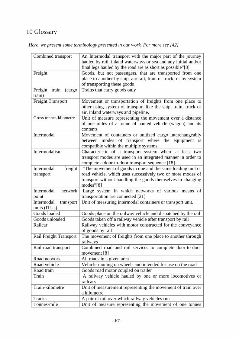
- 67 -

10 Glossary

Here, we present some terminology presented in our work. For more see [42]

Combined transport An Intermodal transport with the major part of the journey hauled by rail, inland waterways or sea and any initial and/or final legs hauled by the road are as short as possible”[8]

Freight Goods, but not passengers, that are transported from one place to another by ship, aircraft, train or truck, or by system of transporting these goods

Freight train (cargo train)

Trains that carry goods only

Freight Transport Movement or transportation of freights from one place to other using system of transport like the ship, train, truck or air, inland waterways and pipeline.

Gross tonnes-kilometre Unit of measure representing the movement over a distance of one miles of a tonne of hauled vehicle (wagon) and its contents

Intermodal Movement of containers or unitized cargo interchangeably between modes of transport where the equipment is compatible within the multiple systems.

Intermodalism Characteristic of a transport system where at least two transport modes are used in an integrated manner in order to complete a door-to-door transport sequence [18].

Intermodal freight transport

“The movement of goods in one and the same loading unit or road vehicle, which uses successively two or more modes of transport without handling the goods themselves in changing modes”[8]

Intermodal network point

Large system in which networks of various means of transportation are connected [21]

Intermodal transport units (ITUs)

Unit of measuring intermodal containers or transport unit.

Goods loaded Goods place on the railway vehicle and dispatched by the railGoods unloaded Goods taken off a railway vehicle after transport by railRailcar Railway vehicles with motor constructed for the conveyance

of goods by railRail Freight Transport The movement of freights from one place to another through

railways Rail-road transport Combined road and rail services to complete door-to-door

movement [8]Road network All roads in a given areaRoad vehicle Vehicle running on wheels and intended for use on the roadRoad train Goods road motor coupled on trailerTrain A railway vehicle hauled by one or more locomotives or

railcarsTrain-kilometre Unit of measurement representing the movement of train over

a kilometreTracks A pair of rail over which railway vehicles runTonnes-mile Unit of measure representing the movement of one tonnes

- 68 -

available one a train wagon over a mileTranshipment Moving of ITUs (intermodal transport units) from one modes

of transportation to another” [8].

Travel sub leg The space between the customer start and end train station which is a subset of train stations along the path of an intermodal line train system.

Wagon Railway vehicle for the transportation of goods