Embed Size (px)
Citation preview

Streaming Submodular Maximization under a k-Set System Constraint
Ran Haba 1 Ehsan Kazemi 2 3 Moran Feldman 4 Amin Karbasi 2
AbstractIn this paper, we propose a novel frameworkthat converts streaming algorithms for monotonesubmodular maximization into streaming algo-rithms for non-monotone submodular maximiza-tion. This reduction readily leads to the currentlytightest deterministic approximation ratio for sub-modular maximization subject to a k-matchoidconstraint. Moreover, we propose the first stream-ing algorithm for monotone submodular maxi-mization subject to k-extendible and k-set systemconstraints. Together with our proposed reduction,we obtain O(k log k) and O(k2 log k) approxima-tion ratio for submodular maximization subjectto the above constraints, respectively. We exten-sively evaluate the empirical performance of ouralgorithm against the existing work in a seriesof experiments including finding the maximumindependent set in randomly generated graphs,maximizing linear functions over social networks,movie recommendation, Yelp location summa-rization, and Twitter data summarization.
1. IntroductionSubmodularity captures an intuitive diminishing returnsproperty where the benefit of an item decreases as the con-text in which it is considered grows. This property naturallyoccurs in many applications where items may represent datapoints, features, actions, etc. Moreover, submodularity is asufficient condition that leads to an efficient optimizationprocedure for many discrete optimization problems. Theabove reasons have led to a surge of applications in machinelearning where the gain of discrete choices shows diminish-ing returns and the optimization can be handled efficiently.Novel examples include non-parametric learning (Mirza-
1Depart. of Mathematics and Computer Science, The OpenUniversity of Israel 2Yale Institute for Network Science, YaleUniversity 3Now at Google, Zürich, Switzerland 4Department ofComputer Science, University of Haifa, Israel. Correspondence to:Ehsan Kazemi <[email protected]>.
Proceedings of the 37 th International Conference on MachineLearning, Online, PMLR 119, 2020. Copyright 2020 by the au-thor(s).
soleiman et al., 2016b), dictionary learning (Das & Kempe,2011), crowd teaching (Singla et al., 2014), regression un-der human assistance (De et al., 2019), sequence selection(Tschiatschek et al., 2017; Mitrovic et al., 2019) interpretingneural networks (Elenberg et al., 2017), adversarial attacks(Lei et al., 2019), fairness (Kazemi et al., 2018), social graphanalysis (Norouzi-Fard et al., 2018), data summarization(Dasgupta et al., 2013; Tschiatschek et al., 2014; Elhamifar& Clara De Paolis Kaluza, 2017; Kirchhoff & Bilmes, 2014;Mitrovic et al., 2018; Kazemi et al., 2020), fMRI parcella-tion (Salehi et al., 2017), and DNA sequencing (Libbrechtet al., 2018).
More formally, a set function f : 2N → R≥0 is called sub-modular if for all sets A ⊆ B ⊆ N and element u /∈ B wehave f(A∪{u})−f(A) ≥ f(B∪{u})−f(B). Moreover,a set function is called monotone if f(A) ≤ f(B) wheneverA ⊆ B. The focus of this paper is on maximizing a gen-eral submodular function (not necessarily monotone). Moreconcretely, we consider a very general form of constrainedsubmodular maximization, i.e.,
OPT = arg maxA∈I
f(A) , (1)
where I represents the set of feasible solutions. For in-stance, when f is monotone and I represents a cardinal-ity/size constraint,1 the celebrated result of (Nemhauseret al., 1978) states that the greedy algorithm achieves ae/(e− 1)-approximation for this problem, which is knownto be optimal (Nemhauser & Wolsey, 1978). In the recentyears, there has been a large body of literature aiming atsolving Problem (1) in the offline/centralized setting undervarious types of feasibility constraints such as matroid, k-matchoid, k-extendible system, and k-set system (formaldefinitions of some of these terms appear in Section 3).
In the offline/centralized setting, the problem of maximizinga (non-monotone) submodular function subject to the abovetypes of constraints is fairly well understood and easy-to-implement algorithms have been proposed. For instance, formaximization under a k-set system constraint, one obtainsan approximation ratio of k + O(
√k) using roughly
√k
invocations of the natural greedy algorithm and an algorithmfor unconstrained submodular maximization. Or, when
1Formally, I contains in this case all subsets of N of size atmost ρ for some value ρ.

Streaming Submodular Maximization under a k-Set System Constraint
the constraint is a k-extendible system, running the greedyalgorithm only once over a carefully subsampled groundset achieves a k + 3 approximation ratio (Feldman et al.,2017). It should also be noted that as is the greedy algorithmfails to provide any constant factor approximation guaranteewhen the submodular function is non-monotone, and thus,the above modifications of it are necessary.
In the streaming setting, when the elements arrive one ata time and the memory footprint is not allowed to growsignificantly with the size of the data, the landscape of con-strained submodular maximization is much less understood.In particular, even for the simple problem of monotone sub-modular maximization subject to a cardinality constraint,the best known approximation guarantee is 2 (Badanidiyuruet al., 2014) (as opposed to e/(e− 1) in the offline setting).Moreover, no algorithm is currently known to achieve anon-trivial guarantee for more complicated constraints suchas k-extendible or k-set system in the streaming setting evenwhen the submodular objective function is monotone.
In this paper, we propose the first streaming algorithm formaximizing a general submodular function (not necessarilymonotone) subject to a general k-set system constraint. Ouralgorithm achieves an O(k2 log k) approximation ratio forthis problem. Moreover, when the constraint reduces toa k-extendible system the approximation guarantee of ourstreaming method improves to a better O(k log k) approxi-mation ratio, nearly matching a lower bound of roughly kdue to (Feldman et al., 2017) that applies even for the offlineversion of the problem. Interestingly, the last approximationratio is a significant improvement even compared to the bestapproximation ratio previously known for the very specialcase of this problem in which the objective function is lin-ear. The current state-of-the-art algorithm for this specialcase, due to (Crouch & Stubbs, 2014), guarantees only anO(k2)-approximation.
With the exception some algorithms designed for the simplecardinality constraint (Alaluf & Feldman, 2019; Badani-diyuru et al., 2014; Ene et al., 2019; Kazemi et al., 2019), allthe streaming algorithms previously suggested for submodu-lar maximization (see (Buchbinder et al., 2014; Chekuriet al., 2015; Chakrabarti & Kale, 2015; Feldman et al.,2018)) have been based on the same basic technique. Thesealgorithms maintain a feasible solution, and update it in thefollowing way. When an element u arrives, the algorithm (1)determines a set of elements that have to be removed fromthe current feasible solution to allow u to be added withoutviolating feasibility, and then (2) decides using some algo-rithm specific rule whether it is beneficial to make this trade(i.e., add u and remove the necessary elements to recoverfeasibility). Our algorithm uses a very different technique ofmaintaining multiple feasible solutions to which elementscan be added (but can never be removed), which is inspired
by the technique of (Crouch & Stubbs, 2014) for maximiza-tion of linear functions subject to k-set systems. Intuitively,each one of the solutions maintained by our algorithm isassociated with a particular importance of elements, and therole of this solution is to collect enough elements of thisimportance. Since we collect elements from each level ofimportance, once the stream ends, the union of the solutionswe maintain is a good enough summary of the stream, andour algorithm is able to pick a feasible subset of this unionwhich is competitive with respect to the optimal solution.
One component of our algorithm is a general frameworkthat is able to convert many streaming algorithms for mono-tone submodular maximization to similar algorithms fornon-monotone submodular maximization. As an immedi-ate consequence of this framework, we get a deterministicstreaming algorithm for maximizing a general (not necessar-ily monotone) submodular function subject to a k-matchoidconstraint, which is an improvement over the state-of-the-art deterministic approximation ratio for this problem dueto (Chekuri et al., 2015). We also compare the empiricalperformance of our algorithm with the existing work and nat-ural baselines in a set of experiments including independentset over randomly generated graphs, maximizing a linearfunction over edges of a graph, movie recommendation,and Yelp location data summarization. In all these applica-tions, the various constraints are modeled as an instance ofa k-extendible or a k-set system.
Before concluding this section, we need to highlight a techni-cal issue. The standard definition of streaming algorithms re-quires them to use poly-logarithmic amount of space, whichis less than the space necessary for keeping a solution toour problem. Thus, no algorithm for this problem aimingto produce a solution (rather than just estimate the valueof the optimal solution) can be a true streaming algorithm.This is true also for all the above mentioned streaming al-gorithms, which are in fact semi-streaming algorithms—asemi-streaming algorithm is an algorithm that processes thedata as a sequence of elements using an amount of spacewhich is nearly linear in the maximum size of a feasiblesolution and typically makes only a single pass over theentire data stream. Since true streaming algorithms arealmost irrelevant to our setting, we ignore the distinctionbetween streaming and semi-streaming algorithms in thispaper and often use the term “streaming algorithm” to referto a semi-streaming algorithm.
Paper Structure. In Section 2, we review the relatedwork. In Section 3, we formally define different types ofconstraints and the notation we use, and then formally statethe technical results that we need. In Section 4, we describeour above mentioned framework for converting streamingalgorithms for monotone submodular maximization intostreaming algorithms for non-monotone submodular max-

Streaming Submodular Maximization under a k-Set System Constraint
imization. Then, in Section 5, we describe and formallyanalyze our algorithm, and in Section 6 we describe the ex-periments we conducted to study the empirical performanceof this algorithm. Most of the proofs for the theoreticalresults are deferred to the Supplementary Material. Anearlier version of this paper, in which the result applies onlyto non-negative linear functions subject to k-extendible con-straints (Feldman & Haba, 2019), appeared on arXiv at thepast under a different title.
2. Related WorkThe study of submodular maximization in the streamingsetting was initialized by the works of Badanidiyuru et al.(2014) and Chakrabarti & Kale (2015). As discussed above,the work of (Chakrabarti & Kale, 2015) was based on atechnique allowing the removal of elements from the solu-tion (also known as preemption). Originally, (Chakrabarti& Kale, 2015) suggested this technique only for constraintsformed by the intersection of k-matroids and a monotonesubmodular objective function, but later works extendedthe use of the technique to the more general class of k-matchoid constraints as well as non-monotone submodularfunctions (Buchbinder et al., 2014; Chekuri et al., 2015;Feldman et al., 2018).
The above mentioned algorithm of Badanidiyuru et al.(2014) works only for the simple cardinality constraint andmonotone submodular objective functions, but provides animproved approximation ratio of 2 for this setting (recently,Feldman et al. (2020) proved the optimality of this approxi-mation factor). The technique at the heart of this algorithmis based on growing a set to which elements can only beadded, which becomes the output solution of the algorithmby the end of the stream (unlike the case in the techniqueof (Crouch & Stubbs, 2014) on which we base our results, inwhich the final solution is obtained by combining multiplesets grown by the algorithm). More recent works improvedthe algorithm of (Badanidiyuru et al., 2014) by improvingits space complexity (Kazemi et al., 2019) and extending itstechnique to non-monotone submodular functions (Alaluf& Feldman, 2019; Ene et al., 2019).
The study of submodular maximization in the offline (cen-tralized) setting is very vast, and thus, we concentrate hereonly on results for general k-extendible or k-set system con-straints. Already in 1978, Fisher et al. (1978) proved thatthe natural greedy algorithm obtains k + 1 approximationfor the problem of maximizing a monotone submodularfunction subject to a k-set system constraint (some of theirproof was given implicitly, and the details were filled inby (Calinescu et al., 2011)). This was recently proved tobe almost optimal. Specifically, Badanidiyuru & Vondrák(2014) proved that no polynomial time algorithm can obtaink−ε approximation for this problem for any constant ε > 0,
and the same inapproximability result was later shown toapply also to k-extendible constraints by (Feldman et al.,2017). As mentioned in Section 1, Feldman et al. (2017)presented the state-of-the-art algorithms for maximizing a(not necessarily monotone) submodular function subject tok-set system and k-extendible constraints. Both algorithmsobtain k + o(k) approximation, which improves over twoprevious results due to (Gupta et al., 2010) and (Mirza-soleiman et al., 2016a) that obtained roughly 3k and 2kapproximation, respectively, for the more general case of ak-set system constraint.
This hierarchy of independence systems (including matroids,k-matchoids, k-extendible systems, and k-set system) isquite rich and expressive. Several recent works have usedthese general constraints for modeling real-world applica-tions. Badanidiyuru et al. (2020) cast text, location, andvideo data summarization tasks to the problem of maxi-mizing a submodular function subject to the interaction ofk-matroids and extend their results to k-matchoids. Mirza-soleiman et al. (2018) and Feldman et al. (2018) studied thevideo and location data summarization applications subjectto k-matchoid constraints in the streaming setting. Feld-man et al. (2017) used a k-extendible constraint to modela movie recommendation application. Mirzasoleiman et al.(2016a) used the intersection of k matroids and ` knapsacksto model several machine learning applications, includingrecommendation systems, image summarization, and rev-enue maximization tasks.
3. Preliminaries and NotationWe begin this section by presenting some notation that weuse in this paper. Then, we formally define some types ofconstraints mentioned in Section 1, and discuss the guaran-tee of a simple greedy algorithm for these constraints.
Given an element u and a setA, we useA+u as a shorthandfor the union A ∪ {u}. We also denote the marginal gainof adding u to A with respect to a set function f : 2N → Rusing f(u | A) , f(A+u)−f(A). Similarly, the marginalgain of adding a set B ⊆ N to another set A ⊆ N isdenoted by f(B | A) , f(B ∪ A)− f(A). Note that thisnotation allows us, for example, to rewrite the definition ofsubmodularity as the requirement that f(u | A) ≥ f(u | B)for every two sets A ⊆ B ⊆ N and element u 6∈ B.
A constraint is defined, for our purposes, as a pair (N , I),whereN is a ground set and I is the collection of all feasiblesubsets of N . All the types of constraints discussed in Sec-tion 1 are independence systems according to the followingdefinition.
Definition 1. Given a ground setN and a collection of setsI ⊆ 2N , the pair (N , I) is an independence system if (i)∅ ∈ I and (ii) for B ∈ I and any A ⊆ B we have A ∈ I.

Streaming Submodular Maximization under a k-Set System Constraint
It is customary to call a setA ⊆ N independent if it belongsto I and dependent if it does not (i.e., it is infeasible). Anindependent set B ∈ I which is maximal with respectto inclusion is called a base; that is, B ∈ I is a base ifA ∈ I and B ⊆ A imply that B = A. Furthermore, anindependent setB ∈ I which is a subset of some setE ⊆ Nis called a base of E if it is a base of the independencesystem (E, 2E ∩ I). Note that this means that a set B is abase of (N , I) if and only if it is a base of N .
With this terminology, we can now define k-set systems.
Definition 2. An independence system (N , I) is a k-setsystem for an integer k ≥ 1 if for every set E ⊆ N , all thebases of E have the same size up to a factor of k (in otherwords, the ratio between the sizes of the largest and smallestbases of E is at most k).
An immediate consequence of the definition of k-set sys-tems is that any base of such a system is a maximum sizeindependent set up to an approximation ratio of k. Thus,one can get a k-approximation for the problem of findinga maximum size set subject to a k-set system constraint byoutputting an arbitrary base of the k-set system, which canbe done using the following simple strategy. Start with theempty solution, and consider the elements of the ground setN in an arbitrary order. When considering an element, addit to the current solution, unless this will make the solutiondependent. We refer to this procedure as the unweightedgreedy algorithm.
Let us now define k-extendible systems. We remind thereader that k-extendible systems are well-known to be arestricted class of k-set systems.
Definition 3. An independence system (N , I) is a k-extendible system for an integer k ≥ 1 if for any two inde-pendent sets S ⊆ T ⊆ N , and an element u 6∈ T such thatS + u ∈ I, there is a subset Y ⊆ T \ S of size at most ksuch that T \ Y + u ∈ I.
Since k-extendible systems are, in particular, k-set systems,the above discussion already implies that the unweightedgreedy algorithm obtains k-approximation for the problemof finding a maximum size independent set in such a system.The following lemma strengthens this observation, and isthe key technical reason that our algorithm has a better ap-proximation guarantee for k-extendible system constraintsthan for k-set system constraints. The proof of the lemmacan be found in Appendix A.1.
Lemma 4. Given a k-extendible set system (N , I), theunweighted greedy algorithm is guaranteed to produce anindependent set B such that k · |B \A| ≥ |A \B| for anyindependent set A ∈ I.
4. A Framework: From Monotone toNon-Monotone Streaming Maximization
Mirzasoleiman et al. (2018) proposed a framework for thefollowing task. Given a streaming2 algorithm for maximiz-ing monotone submodular functions, the framework pro-duces a similar algorithm that works also for non-monotonesubmodular objectives. Unfortunately, however, this frame-work applies only to algorithms satisfying a property which,to the best of our knowledge, is not satisfied by any stream-ing algorithm from the literature (except algorithms thatwork for non-monotone functions by design). In particular,this is the case for the algorithm of Chekuri et al. (2015)explicitly mentioned by (Mirzasoleiman et al., 2018) as anatural fit for their framework. In the rest of this sectionwe discuss this issue in more detail, and then introduce adifferent framework which achieves the same goal (convert-ing algorithms for monotone submodular maximization intoalgorithms for non-monotone submodular maximization),but requires a different property from the input algorithmswhich is satisfied by both existing algorithms from the liter-ature and the new algorithm we suggest in this paper.
The algorithm of (Chekuri et al., 2015) discussed above is astreaming algorithm for maximizing monotone submodularfunctions under a k-matchoid constraint, and Mirzasoleimanet al. (2018) applied their framework to it in order to getsuch an algorithm for non-monotone function. Formally,this framework requires the input streaming algorithm tosatisfy the inequality
f(S) ≥ α · f(S ∪ T ) , (2)
where S as the output of the algorithm, T is an arbitraryfeasible solution and α is a positive value. Unfortunately,the algorithm of (Chekuri et al., 2015) fails to satisfy Eq. (2)for any constant α, so does the algorithms of Buchbinderet al. (2019) and Chakrabarti & Kale (2015). In Appendix Bwe provide examples showing that this is the case for allthese algorithms even under a simple cardinality constraint.
Interestingly, Chekuri et al. (2015) presented, prior to thework of (Mirzasoleiman et al., 2018), an alternative methodto convert their algorithm into a deterministic algorithm fornon-monotone functions based on a technique due to Guptaet al. (2010). The framework we suggest in this paper,can be viewed as a formalization and generalization of thistechnique. As an alternative to the property (2), whichdoes not have counterparts in most of the existing streamingalgorithms, our framework uses the property described byDefinition 5.
2Recall that in this paper we use the term “streaming algorithm”to refer to algorithms that are technically “semi-streaming algo-rithms”, i.e., their space complexity is allowed to be nearly-linearin the size of the output set.

Streaming Submodular Maximization under a k-Set System Constraint
Definition 5. Consider a data stream algorithm3 for maxi-mizing a non-negative submodular function f : 2N → R≥0
subject to a constraint (N , I). We say that such an algo-rithm is an (α, γ)-approximation algorithm, for some α ≥ 1and γ ≥ 0, if it returns two sets S ⊆ A ⊆ N such thatS ∈ I, and for all T ∈ I we have
E[f(T ∪A)] ≤ α · E[f(S)] + γ .
Intuitively, the set S in Definition 5 is the output of thestreaming algorithms, and the set A is the set of “bad” el-ements in the sense that the approximation guarantee ofthe algorithm is with respect to f(OPT ∪ A) rather thanf(OPT ) (for non-monotone functions f(OPT ∪A) mightbe smaller than f(OPT )). Many previous algorithms sat-isfy Definition 5 even with γ = 0, when the set A is theset of all elements that are “seriously” considered by thealgorithm at some point. Unfortunately, however, this setA can be quite large, and therefore, cannot be stored by thealgorithm if we want it to remain a streaming algorithm.Chekuri et al. (2015) described a technique to bypass thisissue by creating a tradeoff between the size of A and thevalue of γ. They do that by guessing the value of the optimalsolution, and discarding elements whose marginal is verysmall compared to the guess. This shrinks the size of theelements that are “seriously” considered, and thus, the sizeof the set A, but requires a positive value for γ representingthe value of elements of OPT that are discarded. By settingthe parameters right, it is possible to keep both γ and |A|reasonably small. The same technique can be used to get asimilar result for the algorithms of (Buchbinder et al., 2019;Chakrabarti & Kale, 2015) as well. More generally, as faras we know, similar modifications can be used to make ev-ery currently existing streaming algorithm for submodularmaximization fit Definition 5, and thus, our framework isapplicable to all these algorithms.
We are now ready to describe the algorithm at the heart ofour framework. This algorithm is given as Algorithm 1,and it assumes access to two procedures: (1) a data streamalgorithm STREAMINGALG for the problem of maximiz-ing a non-negative submodular function f : 2N → R≥0
subject to a constraint (N , I), and (2) an offline algo-rithm CONSTRAINEDALG for the same problem. For thedata stream algorithm STREAMINGALG we use the follow-ing, not very standard, semantics. Algorithm 1 has twoways to call STREAMINGALG. In the first way, every timethat Algorithm 1 would like to pass additional elementsto STREAMINGALG, it calls it with the set of these newelements, and STREAMINGALG updates its internal datastructures accordingly and returns a set including all the
3We remind the reader that a data stream algorithm is anyalgorithm that receives its input in the form of a stream. A (semi-)streaming algorithm is a data stream algorithm whose space com-plexity is nearly linear.
S1
A1
S2
A2
Sr
Ar
S′1 S′2 S′rConstrainedAlg ConstrainedAlg ConstrainedAlg
StreamingAlg1 StreamingAlg2 StreamingAlgr
ui
{ui} D1 D2 Dr−1· · ·
Figure 1. Schematic representation of Algorithm 1.
Algorithm 1: Non-monotone Data Stream Algorithm
1 Input: a positive integer r2 Output: a set S ∈ I3 Initialize r independent copies of STREAMINGALG:
STREAMINGALG(1), . . . , STREAMINGALG(r).4 while there are more elements in the stream do5 Let D0 be a singleton set containing the next
element of the stream.6 for i = 1 to r do
Di ← STREAMINGALG(i)(Di−1).
7 Let D0 ← ∅.8 for i = 1 to r do
[Si, Ai, Di]← STREAMINGALG(i)end(Di−1).
9 Let S′ ← CONSTRAINEDALG(Ai).10 return the set maximizing f among S′ and {Si}ri=1.
elements that it decided to remove from its memory. Inthe second way, once the stream ends, Algorithm 1 callsSTREAMINGALG (denoted by the subscript end) and passesto it any final elements it would like STREAMINGALG to get.STREAMINGALG then process these elements and returnsthree sets: the sets S and A produced by STREAMINGALG(as described in Definition 5) and a setD consisting of all theelements that are still in the memory of STREAMINGALGand did not end up in A. Figure 1 is a graphic representationof the flow of elements within Algorithm 1.
It is clear that Algorithm 1 outputs a feasible solution. Thefollowing theorem gives additional properties of this algo-rithm. Its proof can be found in Appendix A.2.
Theorem 6. Given an (α, γ)-approximation data streamalgorithm STREAMINGALG for maximizing a non-negativesubmodular function subject to some constraint and an of-fline β-approximation algorithm CONSTRAINEDALG forthe same problem. There exists a data stream algorithmreturning a feasible set S that obeys
E[f(S)] ≥ (1− 1/r) · OPT− γα+ β
.
Furthermore,
• this algorithm is deterministic if STREAMINGALG and

Streaming Submodular Maximization under a k-Set System Constraint
CONSTRAINEDALG are both deterministic.
• the space complexity of this algorithm is upperbounded by O(r ·MSTREAMINGALG +MCONSTRAINEDALG),where MSTREAMINGALG and MCONSTRAINEDALG repre-sent the space complexities of their matching al-gorithms under the assumption that the input forSTREAMINGALG is a subset of the full input and theinput for CONSTRAINEDALG is the set A produced bySTREAMINGALG on some such subset.
We note that the algorithm guaranteed by Theorem 6 is astreaming algorithm when STREAMINGALG is a stream-ing algorithm, the algorithm CONSTRAINEDALG is anearly-linear space algorithm and r is upper bounded bya poly-log function (note that the sets Si and Ai are pro-duced by STREAMINGALG, and thus, their space complex-ity is already accounted for by the space complexity ofSTREAMINGALG).
In Appendix C we show that by plugging one of the versionsof the algorithm of Chekuri et al. (2015) into our frame-work it is straightforward to get a deterministic streamingalgorithm for the problem of maximizing a non-negative(not necessarily monotone) submodular function subjectto a k-matchoid constraint whose approximation ratio is(5 + 15ε)k + O(
√k) for every constant ε > 0, which is
an improvement over the guarantee of the previous state-of-the-art deterministic streaming algorithm for this problem(also due to (Chekuri et al., 2015)) which has an approx-imation guarantee of 8k + γ, where γ is the best offlineapproximation ratio for the same problem.
5. Streaming Submodular Maximizationunder a k-System Constraint
In this section, we formally prove our results for the prob-lem of maximizing a non-negative submodular functionf : 2N → R≥0 subject to a k-set system and k-extendiblesystem constraint (N , I). A simple version of the algorithmwe use to prove these results is given as Algorithm 2. Thisversion assumes pre-access to a value ρ equal to the size ofthe largest independent set in I and a threshold τ estimatingthe valueM = maxu∈N ,{u}∈I f({u}). In Appendix D, wepresent a more involved version of our algorithm that doesnot need this pre-access, but has a space complexity largerthan that of Algorithm 2 by a factor ofO(log ρ+log k)—theapproximation guarantee remains unchanged.
Intuitively, Algorithm 2 maintains ` independent sets Ei,where each one of these sets corresponds to a differentrange of marginal contributions: the larger i, the smallerthe marginal contributions Ei is associated with. Whenan element u arrives, the algorithm calculates the marginalcontribution m(u) of u with respect to the union of the
Ei sets,4 and then adds u to the Ei corresponding to thismarginal contribution, unless this violates the independenceof this Ei. Once the entire input has been processed, thealgorithm combines the Ei sets into h possible output setsT0, T1, . . . , Th−1. Each output sets Tj is constructed bygreedily taking elements from the Ei sets obeying i ≡ j(mod h) (the algorithm scans the sets obeying this conditionin an increasing i order, which is a decreasing order withrespect to the marginal contributions associated with thesesets). The final output of the algorithm is simply the best setamong the sets T0, T1, . . . , Th−1.
Algorithm 2: Streaming Algorithm for k-set Systems
1 Input: a threshold τ ∈ [M, 2M ], the size ρ of thelargest independent set, and the parameter k of theconstraint. // M = maxu∈N ,{u}∈I f({u}).
2 Output: a solution T ∈ I3 Let `← blog2(4ρ)c and h← dlog2(2k + 1)e.4 for i = 0 to ` do Initialize Ei ← ∅.5 for every element u arriving do
/* Adds u to a set Ei(u) based on its
marginal gain. */
6 Let m(u)← f(u | ∪`i=0Ei
).
7 if m(u) > 0 then Let i(u)← blog2(τ/m(u))celse Let i(u)←∞.
8 if 0 ≤ i(u) ≤ ` and Ei(u) + u ∈ I then UpdateEi(u) ← Ei(u) + u.
9 for j = 0 to h− 1 do10 Let i← j and Tj ← ∅.11 while i ≤ ` do12 while there is an element u ∈ Ei such that
Tj + u ∈ I do Update Tj ← Tj + u.13 i← i+ h. // Greedily generates
solution Tj from sets Ei for i ≡ j(mod h).
14 return the set T maximizing function f among setsT0, T1, · · · , Th−1.
Let’s denote E = ∪`i=0Ei. It is not difficult to argue thatthe value of f(E) is large. In Lemma 7, we show that thevalue of the output set of the algorithm is proportional tof(E) subject to a k-set system constraint.5
Lemma 7. If (N , I) is a k-set system, then Algorithm 2returns a set T such that
f(T ) ≥ f(E ∪ U)− τ/44kh(2k + 1)
=f(E ∪ U)− τ/4O(k2 log k)
4The notationm(u) might suggest that the valuem(u) dependsonly on the identity of the element u. However, this is not the case.In fact, m(u) might depend also on the set of elements that arrivedbefore u and the order of their arrival.
5In the supplementary material, we provide a stronger versionof this result for k-extendible constraints.

Streaming Submodular Maximization under a k-Set System Constraint
for every set U ∈ I.
Following (see Lemma 8) is the key result that we use toprove Lemma 7. This lemma relates the value of f(Tj) tothe sum of the m(u) values of the elements u that belongto the sets Ei that are combined to create Tj (recall thatthese are exactly the sets Ei for which i ≡ j (mod h)).Intuitively, the lemma holds because when Algorithm 2adds elements of a set Ei to a set Tj , this increases the sizeof the set Tj to at least Ei/k (since the constraint is k-setsystem). Thus, either about 1/k of the elements of Ei areadded to Tj , or the size of Tj before the addition of theelements of Ei is already significant compared to the sizeof Ei. Moreover, in the latter case, the elements of Tj canpay for the elements of Ei that they have blocked becausethey all have a relatively high value (as they originate in aset Ei′ for some i′ ≤ i− h).Lemma 8. If (N , I) is a k-set system, then for every integer0 ≤ j < h we have
f(Tj | ∅) ≥ 1
4k·∑
0≤i≤`i≡j(mod h)
∑
u∈Ei
m(u) .
From the result of Lemma 7, we can directly guarantee theperformance of our algorithm for monotone submodularfunctions. Furthermore, Lemma 7 implies that Algorithm 2is a (4kh(2k + 1), τ/4)-approximation data stream algo-rithm subject to a k-set system constraint.6 Therefore, wecan use the framework of Algorithm 1 to make this algo-rithm suitable for non-monotone submodular functions. Thefollowing two theorems describe the guarantees we providefor Algorithm 2, and their complete proofs can be found inAppendix A.3.Theorem 9. There is a streaming O(k2 log k) = O(k2)-approximation algorithm for maximizing a non-negativesubmodular function subject to a k-set system constraint.Theorem 10. There is a streaming O(k log k) = O(k)-approximation algorithm for maximizing a non-negativesubmodular function subject to a k-extendible system con-straint.
6. ExperimentsIn this section, we compare our proposed algorithms (bothmonotone and non-monotone versions) with two othergroups of algorithms: other streaming algorithms and state-of-the-art offline algorithms.
We consider three baseline streaming algorithms: i) TheStreaming-Greedy algorithm: this algorithm keeps a so-lution S which is initially set to the empty set. For every
6In the supplementary material, we prove that Algorithm 2 is a(4h(2k + 1), τ/4)-approximation data stream algorithm subjectto a k-extendible constraint.
incoming element u, it is added to the set S if this doesnot violate feasibility (i.e., S ∪ {u} ∈ I). ii) The Pre-emption algorithm: Inspired by the streaming algorithmsof (Chekuri et al., 2015; Buchbinder et al., 2019), we con-sider a heuristic preemptive algorithm. For every incomingelement u, given that S is the current solution, this algo-rithm generates a set U ⊆ S such that (S ∪ {u}) \ Uis feasible under the non-knapsack constraints. The ele-ment u is then added to the solution in exchange for theelements of U if this does not violate the knapsack con-straints and the exchange is beneficial in the sense that f(u |S) ≥∑u′∈U f(u′ : S), where f(u′ : S) = f(u′ | S′) forS′ = {s ∈ S : element s arrived before u′}. For more de-tail refer to (Chekuri et al., 2015; Feldman et al., 2018). iii)The Sieve-Streaming algorithm: this heuristic algorithmis implemented based on the ideas of (Badanidiyuru et al.,2014). In the first step, it finds an accurate estimation ofOPT. Then, each incoming element u is added to the solu-tion S if S ∪ {u} ∈ I and f(u | S) ≥ OPT/(2ρ), where ρis the maximum cardinality of a feasible solution.
For the offline algorithms we consider 1) the vanilla greedyalgorithm (referred to as Greedy), 2) Fast (Badanidiyuru& Vondrák, 2014) and FANTOM (Mirzasoleiman et al.,2016a). Both Fast and FANTOM are designed to maxi-mize submodular functions under a k-set system constraintcombined with ` knapsack constraints.
Sections 6.1 and 6.2 compare the above algorithms on tasksof maximizing linear and cut objective functions over in-stances produced using synthetic and real-world data, re-spectively. Then, in Section 6.3 and Appendices E.4 and E.5,we evaluate the performance of the same algorithms on threedifferent real-world applications. In a movie recommenda-tion system application, we are given movie ratings fromusers, and our goal is to recommend diverse movies fromdifferent genres. In a Yelp location summarization appli-cation, we are given thousands of business locations withseveral related attributes. Our objective is to find a goodsummary of the locations from six different cities. In a thirdapplication, our goal is to generate real-time summaries forTwitter feeds of several news agencies.
6.1. Independent set
In the experiments of this section we define submodularfunctions over the nodes of a given graph G = (V,E),and consider the maximization of such functions subjectto an independent set constraint, i.e., we are not allowedto select a set of vertices if there is any edge of the graphconnecting any two of these vertices. It is easy to showthat this constraint is a dmax-extendible system, where dmax
is the maximum degree in graph G. In our experimentsin this section, we use two types of synthetically gener-ated random graphs: Erdos Rény graphs (Erdos & Rény,

Streaming Submodular Maximization under a k-Set System Constraint
1960) and Watts–Strogatz graphs (Watts & Strogatz, 1998).For the Erdos Rény graphs we vary in our experimentsthe probability p that each possible edge is included in thegraph (independently from every other edge), and for theWatts-Strogatz graphs we vary the rewiring probability β.The number of nodes is set to n = 2000 in all the graphs,and in the Watts–Strogatz model each node is connected tok = 100 nearest neighbors in the ring structure.
In our first experiment of the section, we study the maxi-mization of the following monotone linear function f(S) =∑u∈S wu, where S ⊆ V and wu is the weight of node
u ∈ S. Figs. 2a and 2b compare different algorithms foroptimizing this function over a random graph chosen fromthe above discussed random graph models. We observethat our proposed algorithm consistently outperforms theother baseline streaming algorithms. We also observe thatthe performance our algorithm is comparable with (or evenbetter at times) the greedy algorithm, which is provablyoptimal for the maximization of linear functions subject tok-extendible constraints (Feldman et al., 2017).
In the second experiment, we study the non-monotone sub-modular graph-cut function: f(S) =
∑u∈S
∑v∈V \S wu,v,
where wu,v is the weight of the edge e = (u, v). Again, inFigs. 2c and 2d we observe that the solutions provided byour algorithms are clearly better than those produced by theother streaming algorithms. Furthermore, the non-monotoneversion of our algorithm always outperforms the monotonealgorithm. We also note that the for this non-monotonesubmodular function, the vanilla greedy algorithm performsvery poorly (which is consistent with the lack of a theoreticalguarantee for this algorithm for such functions).
6.2. Graph Planarity with Knapsack
In the experiment of this section, our objective is to maxi-mize a linear function over the edges of a graphG = (V,E).For the constraint, we require that an independent set ofedges corresponds to a planar sub-graph of G, and in addi-tion, it satisfies a given knapsack constraint. We remind thereader that a graph is planar if it can be embedded in theplane. Furthermore, a knapsack constraint is defined by acost function c : N → R≥0, and we say that a set S ⊆ Nsatisfies the knapsack constraint if c(S) =
∑e∈S c(e) ≤ b
for a given knapsack budget b. In Appendix E.1 we explainwhy the above mentioned constraint is k-set system for a(relatively) modest value of k.7.
For the objective function f , we use the monotone linearfunction: f(S) =
∑e∈S we ∀S ⊆ E, where we is the
weight of edge e ∈ S, and for simplicity, we set all theseweights to 1. The knapsack cost of each edge e = (u, v) ∈
7We would like to thank Chandra Chekuri for pointing outsome parts of this explanation to us.
E is chosen to be proportional to max(1, du− q), where duis the degree of node u in graph G and q = 6, and the costsare normalized so that
∑e∈E ce = |V |, where ce represents
the knapsack cost of edge e.
In the experiment, we use two real-world networks from(Leskovec & Krevl, 2014) as the graph, and vary the knap-sack budget between 0 and 1 (note that the normalizationgives this range of budgets an intuitive meaning). In Figs. 3aand 3b we compare the performance of our streaming algo-rithm with the performance of Streaming Greedy and SieveStreaming. One can observe that our algorithm outperformsthe two other baselines. Due to the prohibitive computa-tional complexity of the offline algorithms, we do not reporttheir results for this experiment. Furthermore, as it is notclear how to execute a preemptive streaming algorithm un-der a planarity constraint, we did not include a version ofthe Preemption algorithm in this experiment. Further exper-iments in this setting can be found in Appendix E.2.
6.3. Movie Recommendation
In the movie recommendation application, our goal is toselect a diverse set of movies subject to constraints that canbe adjusted by the user. The dataset for this experiment con-tains 1793 movies from the genres: Adventure, Animation,and Fantasy (note that a single movie may be identified withmultiple genres). The user may specify an upper limit m onthe number of movies in the set we recommend for them, aswell as an upper limitmi on the number of movies from eachgenre. For simplicity, we use a single value for allmi and re-fer to this value as the genre limit. It is easy to show that thisset of constraints forms a 3-extendible system. In addition,we enforce two knapsack constraints. For the first knapsackconstraint c1, the cost of each movie is proportional to theabsolute difference between the release year of the movieand the year 1985 (the implicit goal of this constraint is topick movies with a release year which is as close as possibleto the year 1985). For the second knapsack constraint c2, thecost of each movie is proportional to the difference betweenthe maximum possible rating (which is 10) and the rating ofthe particular movie—here the goal is to pick movies withhigher ratings. More formally, for a movie v ∈ N , we have:c1(v) ∝ |1985− yearv| and c2(v) ∝ (10− ratingv). Here,yearv and ratingv , respectively, denote the release year andIMDb rating of movie v. We normalize the costs in bothknapsacks constraints so that the average cost of each movieis 1/10, i.e.,
∑v∈N ci(V )
|N | = 1/10, and we set the knapsackbudgets to 1; which intuitively means that a feasible set cancontain no more than about 10% of the movies.
In our experiments, we try to maximize two kinds of ob-jective functions (each trying to capture diversity in a dif-ferent way) subject to these constraints, and we vary theupper limitm on the number of movies in the recommended

Streaming Submodular Maximization under a k-Set System Constraint
0.0 0.1 0.2 0.3 0.4
Edge probabiltiy p
0
25
50
75
100
125
Ob
ject
ive
valu
e
Ours (monotone)Streaming-Greedy Greedy Preemption Sieve-Streaming
(a) Erdos Rény (linear)
0.0 0.1 0.2 0.3 0.4
Rewiring probabiltiy β
20
30
40
50
60
Ob
ject
ive
valu
e
Ours (monotone)Streaming-Greedy Greedy Preemption Sieve-Streaming
(b) Watts–Strogatz (linear)
0.0 0.1 0.2 0.3 0.4
Edge probabiltiy p
0
2000
4000
6000
Ob
ject
ive
valu
e
Ours (monotone)Ours (non-monotone)Streaming-Greedy Greedy Preemption Sieve-Streaming
(c) Erdos Rény (cut)
0.0 0.1 0.2 0.3 0.4
Rewiring probabiltiy β
0
1000
2000
3000
4000
5000
Ob
ject
ive
valu
e
Ours (monotone)Ours (non-monotone) Streaming-Greedy Greedy Preemption Sieve-Streaming
(d) Watts–Strogatz (cut)
Figure 2. For Erdos Rény graphs p is the probability of having an edge between any two nodes. For Watts–Strogatz graphs β is theprobability of rewiring of each edge.
0.2 0.4 0.6 0.8 1.0
Knapsack budget
20
40
60
80
100
Ob
ject
ive
valu
e
Ours (monotone)Streaming-Greedy Sieve-Streaming
(a) EU Email
0.2 0.4 0.6 0.8 1.0
Knapsack budget
50
100
150
Ob
ject
ive
valu
e
Ours (monotone)Streaming-Greedy Sieve-Streaming
(b) Facebook ego network
5 10 15 20 25
Maximum number of allowed elements
10000
20000
30000
40000
Ob
ject
ive
valu
e
Ours (monotone)
Ours (non-monotone)
Streaming-Greedy
Sieve-Streaming
Fast
FANTOM
(c) Non-monotone function
5 10 15 20 25
Maximum number of allowed elements
0
1
2
3
4
Ora
cle
call
s
×106
Ours (monotone)
Ours (non-monotone)
Streaming-Greedy
Sieve-Streaming
Fast
FANTOM
(d) Non-monotone function
Figure 3. (a) and (b): Planarity with knapsack (linear objective function). (c) and (d): Movie recommendation with two knapsacks.
set of movies. Both objective functions are based a setof attributes calculated for each movie using the methoddescribed in (Lindgren et al., 2015), and both objectivefunctions are non-negative and submodular. However, oneof them is monotone, and the other is not (guaranteed tobe) monotone. The experimental result for the monotonefunction is given in Appendix E.3.
An intuitive utility function for choosing a diverse set ofmovies S is the following not necessarily monotone sub-modular function
f(S) =∑
i∈S
∑
j∈NMi,j −
∑
i∈S
∑
j∈SMi,j , (3)
whereN is the set of all movies andMi,j is the non-negativesimilarity score between movies i, j ∈ N as defined in theprevious section. It is beneficial to note that the first term isa sum-coverage function that captures the representativenessof the selected set, and the second term is a dispersion func-tion penalizing similarity within S (Feldman et al., 2017).
In our experiment with this function as the object, we setthe genre limit to 20. In Figs. 3c and 3d, we observe that i)our streaming algorithm returns solutions with higher utili-ties compared to the baseline streaming algorithms, ii) thenon-monotone version of our algorithm clearly outperformsthe monotone one for this non-monotone function, and iii)the quality of the solutions returned by our algorithms iscomparable with the quality obtained by offline algorithms.
7. ConclusionIn this paper, we have proposed a novel framework forconverting streaming algorithms for monotone submodularmaximization into streaming algorithms for non-monotonesubmodular maximization, which immediately led us to thecurrently tightest deterministic approximation ratio for sub-modular maximization subject to a k-matchoid constraint.We also proposed the first streaming algorithm for mono-tone submodular maximization subject to k-extendible andk-set system constraints, which (together with our proposedframework), yields approximation ratios of O(k log k) andO(k2 log k) for maximization of general non-negative sub-modular functions subject to the above constraints, respec-tively. Finally, we extensively evaluated the empirical perfor-mance of our algorithm against the existing work in a seriesof experiments including finding the maximum independentset in randomly generated graphs, maximizing linear func-tions over social networks, movie recommendation, Yelplocation summarization, and Twitter data summarization.
AcknowledgementsThe research of Moran Feldman and Ran Haba was partiallysupported by ISF grant 1357/16. Amin Karbasi is partiallysupported by NSF (IIS- 1845032), ONR (N00014-19-1-2406), and AFOSR (FA9550-18-1-0160).

Streaming Submodular Maximization under a k-Set System Constraint
ReferencesAlaluf, N. and Feldman, M. Making a sieve random:
Improved semi-streaming algorithm for submodularmaximization under a cardinality constraint. CoRR,abs/1906.11237, 2019.
Badanidiyuru, A. and Vondrák, J. Fast algorithms for maxi-mizing submodular functions. In ACM-SIAM symposiumon Discrete algorithms (SODA), pp. 1497–1514, 2014.
Badanidiyuru, A., Mirzasoleiman, B., Karbasi, A.,and Krause, A. Streaming Submodular Maximiza-tion:Massive Data Summarization on the Fly. In Inter-national Conference on Knowledge Discovery and DataMining, KDD, pp. 671–680, 2014.
Badanidiyuru, A., Karbasi, A., Kazemi, E., and Vondrák,J. Submodular maximization through barrier functions.arXiv preprint arXiv:2002.03523, 2020.
Buchbinder, N., Feldman, M., Naor, J., and Schwartz, R.Submodular Maximization with Cardinality Constraints.In SODA, pp. 1433–1452, 2014.
Buchbinder, N., Feldman, M., and Schwartz, R. OnlineSubmodular Maximization with Preemption. ACM Trans.Algorithms, 15(3):30:1–30:31, 2019.
Calinescu, G., Chekuri, C., Pál, M., and Vondrák, J. Max-imizing a monotone submodular function subject to amatroid constraint. SIAM J. Comput., 40(6):1740–1766,2011.
Chakrabarti, A. and Kale, S. Submodular maximizationmeets streaming: matchings, matroids, and more. Math.Program., 154(1–2):225–247, 2015.
Chekuri, C., Gupta, S., and Quanrud, K. Streaming algo-rithms for submodular function maximization. In ICALP,pp. 318–330, 2015.
Crouch, M. and Stubbs, D. M. Improved streaming algo-rithms for weighted matching, via unweighted matching.In APPROX, pp. 96–104, 2014.
Das, A. and Kempe, D. Submodular meets spectral: greedyalgorithms for subset selection, sparse approximationand dictionary selection. In International Conferenceon International Conference on Machine Learning, pp.1057–1064, 2011.
Dasgupta, A., Kumar, R., and Ravi, S. Summarizationthrough submodularity and dispersion. In Annual Meet-ing of the Association for Computational Linguistics, pp.1014–1022, 2013.
De, A., Koley, P., Ganguly, N., and Gomez-Rodriguez,M. Regression Under Human Assistance. CoRR,abs/1909.02963, 2019.
Elenberg, E. R., Dimakis, A. G., Feldman, M., and Karbasi,A. Streaming Weak Submodularity: Interpreting NeuralNetworks on the Fly. In Advances in Neural InformationProcessing Systems, pp. 4047–4057, 2017.
Elhamifar, E. and Clara De Paolis Kaluza, M. Online sum-marization via submodular and convex optimization. InProceedings of the IEEE Conference on Computer Visionand Pattern Recognition, pp. 1783–1791, 2017.
Ene, A., Nguyen, H. L., and Suh, A. An optimal streamingalgorithm for non-monotone submodular maximization.CoRR, abs/1911.12959, 2019.
Erdos, P. and Rény, A. On the Evolution of Random Graphs.Publ. Math. Inst. Hungary. Acad. Sci., 5:17–61, 1960.
Feldman, M. and Haba, R. Almost Optimal Semi-streamingMaximization for k-Extendible Systems. arXiv preprintarXiv:1906.04449, 2019.
Feldman, M., Harshaw, C., and Karbasi, A. Greed is good:Near-optimal submodular maximization via greedy opti-mization. In COLT, pp. 758–784, 2017.
Feldman, M., Karbasi, A., and Kazemi, E. Do less, get more:Streaming submodular maximization with subsampling.In NeurIPS, pp. 730–740, 2018.
Feldman, M., Norouzi-Fard, A., Svensson, O., and Zen-klusen, R. The one-way communication complexity ofsubmodular maximization with applications to streamingand robustness. In Symposium on Theory of Computing(STOC), pp. 1363–1374, 2020.
Fisher, M., Nemhauser, G., and Wolsey, L. An analysis ofapproximations for maximizing submodular set functions–II. Mathematical Programming, 8:73–87, 1978.
Frieze, A. M. A cost function property for plant locationproblems. Mathematical Programming, 7(1):245–248,1974.
Gupta, A., Roth, A., Schoenebeck, G., and Talwar, K. Con-strained Non-monotone Submodular Maximization: Of-fline and Secretary Algorithms. In WINE, pp. 246–257,2010.
Herbrich, R., Lawrence, N. D., and Seeger, M. Fast sparseGaussian process methods: The informative vector ma-chine. In Advances in Neural Information ProcessingSystems, pp. 625–632, 2003.
Kazemi, E., Zadimoghaddam, M., and Karbasi, A. Scal-able Deletion-Robust Submodular Maximization: DataSummarization with Privacy and Fairness Constraints. InInternational Conference on Machine Learning (ICML),pp. 2549–2558, 2018.

Streaming Submodular Maximization under a k-Set System Constraint
Kazemi, E., Mitrovic, M., Zadimoghaddam, M., Lattanzi,S., and Karbasi, A. Submodular Streaming in All ItsGlory: Tight Approximation, Minimum Memory andLow Adaptive Complexity. In International Conferenceon Machine Learning (ICML), pp. 3311–3320, 2019.
Kazemi, E., Minaee, S., Feldman, M., and Karbasi, A. Regu-larized submodular maximization at scale. arXiv preprintarXiv:2002.03503, 2020.
Kirchhoff, K. and Bilmes, J. Submodularity for data selec-tion in statistical machine translation. In Proceedings ofEMNLP, 2014.
Krause, A. and Golovin, D. Submodular Function Maxi-mization. In Tractability: Practical Approaches to HardProblems. Cambridge University Press, 2012.
Lei, Q., Wu, L., Chen, P.-Y., Dimakis, A., Dhillon, I., andWitbrock, M. Discrete Adversarial Attacks and Submodu-lar Optimization with Applications to Text Classification.Systems and Machine Learning (SysML), 2019.
Leskovec, J. and Krevl, A. SNAP Datasets: StanfordLarge Network Dataset Collection. http://snap.stanford.edu/data, June 2014.
Libbrecht, M. W., Bilmes, J. A., and Noble, W. S. Choosingnon-redundant representative subsets of protein sequencedata sets using submodular optimization. Proteins: Struc-ture, Function, and Bioinformatics, 2018. ISSN 1097-0134.
Lindgren, E. M., Wu, S., and Dimakis, A. G. Sparse andgreedy: Sparsifying submodular facility location prob-lems. In NIPS Workshop on Optimization for MachineLearning, 2015.
Mirzasoleiman, B., Karbasi, A., Sarkar, R., and Krause,A. Distributed Submodular Maximization: IdentifyingRepresentative Elements in Massive Data. In Advances inNeural Information Processing Systems, pp. 2049–2057,2013.
Mirzasoleiman, B., Badanidiyuru, A., and Karbasi, A. FastConstrained Submodular Maximization: PersonalizedData Summarization. In ICML, pp. 1358–1367, 2016a.
Mirzasoleiman, B., Karbasi, A., Sarkar, R., and Krause,A. Distributed Submodular Maximization. Journal ofMachine Learning Research, 17:238:1–238:44, 2016b.
Mirzasoleiman, B., Jegelka, S., and Krause, A. StreamingNon-Monotone Submodular Maximization: PersonalizedVideo Summarization on the Fly. In AAAI Conference onArtificial Intelligence,, pp. 1379–1386, 2018.
Mitrovic, M., Kazemi, E., Zadimoghaddam, M., and Kar-basi, A. Data Summarization at Scale: A Two-StageSubmodular Approach. In International Conference onMachine Learning (ICML), pp. 3593–3602, 2018.
Mitrovic, M., Kazemi, E., Feldman, M., Krause, A., andKarbasi, A. Adaptive sequence submodularity. In Ad-vances in Neural Information Processing Systems, pp.5352–5363, 2019.
Nemhauser, G. L. and Wolsey, L. A. Best algorithms forapproximating the maximum of a submodular set func-tion. Mathematics of Operations Research, 3(3):177–188,1978.
Nemhauser, G. L., Wolsey, L. A., and Fisher, M. L. Ananalysis of approximations for maximizing submodularset functions–I. Mathematical Programming, 14(1):265–294, 1978.
Norouzi-Fard, A., Tarnawski, J., Mitrovic, S., Zandieh,A., Mousavifar, A., and Svensson, O. Beyond 1/2-approximation for submodular maximization on massivedata streams. In International Conference on MachineLearning (ICML), pp. 3826–3835, 2018.
Salehi, M., Karbasi, A., Scheinost, D., and Constable, R. T.A Submodular Approach to Create Individualized Parcel-lations of the Human Brain. In MICCAI, pp. 478–485,2017.
Singla, A., Bogunovic, I., Bartók, G., Karbasi, A., andKrause, A. Near-Optimally Teaching the Crowd to Clas-sify. In International Conference on Machine Learning(ICML), 2014.
Tschiatschek, S., Iyer, R. K., Wei, H., and Bilmes, J. A.Learning mixtures of submodular functions for imagecollection summarization. In Advances in neural infor-mation processing systems, pp. 1413–1421, 2014.
Tschiatschek, S., Singla, A., and Krause, A. Selectingsequences of items via submodular maximization. InAAAI Conference on Artificial Intelligence, 2017.
Watts, D. J. and Strogatz, S. H. Collective dynamics of‘small-world’networks. nature, 393(6684):440, 1998.
Yelp. Yelp Academic Dataset. https://www.kaggle.com/yelp-dataset/yelp-dataset, 2019a.
Yelp. Yelp Dataset. https://www.yelp.com/dataset, 2019b.

Streaming Submodular Maximization under a k-Set System Constraint
A. ProofsA.1. Proof of Lemma 4
In this section, we restate Lemma 4 and then prove it.
Lemma 4. Given a k-extendible set system (N , I), the unweighted greedy algorithm is guaranteed to produce an indepen-dent set B such that k · |B \A| ≥ |A \B| for any independent set A ∈ I.
Proof. Let us denote the elements of B \A by x1, x2, . . . , xm in an arbitrary order. Using these elements, we recursivelydefine a series of independent sets A0, A1, . . . , Am. The set A0 is simply the set A. For 1 ≤ i ≤ m, we define Ai usingAi−1 as follows. Since (N , I) is a k-extendible system and the subsets Ai−1 and Ai−1 ∩B+xi ⊆ B are both independent,there must exist a subset Yi ⊆ Ai−1 \ (Ai−1 ∩ B) = Ai−1 \ B such that |Yi| ≤ k and Ai−1 \ Yi + xi ∈ I. Using thesubset Yi, we now define Ai = Ai−1 \ Yi + xi. Note that by the definition of Yi, Ai ∈ I as promised. Furthermore, sinceYi ∩ B = ∅ for each 0 ≤ i ≤ m, we know that (A ∪ {x1, x2, . . . , xm}) ∩ B ⊆ Am, which implies B ⊆ Am because{x1, x2, . . . , xm} = B \ A. However, B, as the output of the unweighted greedy algorithm, must be an inclusion-wisemaximal independent set (i.e., a base), and thus, it must be in fact equal to the independent set Am containing it.
Let us now denote Y =⋃mi=1 Yi, and consider two different ways to bound the number of elements in Y . On the one hand,
since every set Yi includes up to k elements, we get |Y | ≤ km = k · |B \ A|. On the other hand, the fact that B = Amimplies that every element of A \B belongs to Yi for some value of i, and therefore, |Y | ≥ |A \B|. The lemma now followsby combining these two bounds.
A.2. Proof of Theorem 6
In this section we prove Theorem 6. For convenience, we begin by restating the theorem itself.
Theorem 6. Given an (α, γ)-approximation data stream algorithm STREAMINGALG for maximizing a non-negativesubmodular function subject to some constraint and an offline β-approximation algorithm CONSTRAINEDALG for the sameproblem. There exists a data stream algorithm returning a feasible set S that obeys
E[f(S)] ≥ (1− 1/r) · OPT− γα+ β
.
Furthermore,
• this algorithm is deterministic if STREAMINGALG and CONSTRAINEDALG are both deterministic.
• the space complexity of this algorithm is upper bounded by O(r · MSTREAMINGALG + MCONSTRAINEDALG), whereMSTREAMINGALG and MCONSTRAINEDALG represent the space complexities of their matching algorithms under the as-sumption that the input for STREAMINGALG is a subset of the full input and the input for CONSTRAINEDALG is theset A produced by STREAMINGALG on some such subset.
Recall that our goal is to show that Algorithm 1 has the properties guaranteed by the theorem. The following observationshows that this is the case for the space complexity.
Observation 11. The space complexity of Algorithm 1 is upper bounded byO(r ·MSTREAMINGALG +MCONSTRAINEDALG), whereMSTREAMINGALG and MCONSTRAINEDALG represent the space complexities of their matching algorithms under the assumptionthat the input for STREAMINGALG is a subset of the full input and the input for CONSTRAINEDALG is the A set producedby STREAMINGALG on some such subset.
Proof. Note that every set assigned to a variable Di by Algorithm 1 is either an input set for some copy of STREAMINGALGor an output set of such a copy. Furthermore, any such set is either ignored or fed immediately after construction to some copyof STREAMINGALG. Thus, the space complexity required for these sets is upper bounded by the space complexity requiredfor the r copies of STREAMINGALG used by Algorithm 1, which isO(r ·MSTREAMINGALG). Additionally, since the sets Si andAi are the final outputs of these copies of STREAMINGALG, we get they can also be stored usingO(r ·MSTREAMINGALG) space.Finally, the set S′ is a subset of
⋃ri=1Ai, and therefore, does not require more space than the sets Ai. Combining all the
above, we get that the space complexity of Algorithm 1—excluding the space required for running CONSTRAINEDALG—isat most O(r ·MSTREAMINGALG).

Streaming Submodular Maximization under a k-Set System Constraint
To complete the proof of Theorem 6, it remains to analyze the approximation guarantee of Algorithm 1. Towards this goal,we need the following known lemma.
Lemma 12 (Lemma 2.2 of (Buchbinder et al., 2014)). Let g : 2N → R≥0 be a non-negative submodular function, and letB be a random subset of N containing every element of N with probability at most q (not necessarily independently). Then,E[g(B)] ≥ (1− q) · g(∅).
Lemma 13. Assume STREAMINGALG is an (α, γ)-approximation algorithm and CONSTRAINEDALG is an offline β-approximation algorithm. Then, Algorithm 1 returns a solutions S such that
E[f(S)] ≥ (1− 1/r) · OPT− γα+ β
.
Proof. Let S∗ be an arbitrary optimal solution, i.e., a set obeying S∗ ∈ I and f(S∗) = OPT. For every integer 1 ≤i ≤ r, we denote by Ni the set of elements that STREAMINGALG(i) has received. Note that we have N1 = N andNi = N \ (∪1≤j≤i−1Aj) for 2 ≤ i ≤ r since STREAMINGALG(i) outputs every element that it gets and does not end up inAi as an element of Di at some point. Since Ai is a subset of Ni, this implies that the sets A1, A2, . . . , Ar are disjoint.
Let us define now A to be a uniformly random set from {A1, A2, . . . , Ar}, and g(S) = f(S ∪ S∗). Then,
1
r
r∑
i=1
f(Ai ∪ S∗) = EA[f(A ∪ S∗)] = EA[g(A)] ≥(
1− 1
r
)· g(∅) =
(1− 1
r
)· f(S∗) ,
where the notation EA stands for expectation over the random choice of A out of {A1, A2, . . . , Ar} (but not over anyrandomness that might be introduced by STREAMINGALG), and the inequality results from Lemma 12 because (i) everyelement of N belongs to A with probability at most 1
r since the sets Ai are disjoint, and (ii) g is a non-negative submodularfunction on its own right.
Let us now define A′ =⋃ri=1Ai. Using this notation, we get from the last inequality
(r − 1) · OPT = (r − 1) · f(S∗) ≤r∑
i=1
f(Ai ∪ S∗) ≤r∑
i=1
[f(Ai ∪ (S∗ \A′)) + f(S∗ ∩A′)] ,
where the second inequality follow from the submodularity and non-negativity of f . Observe now that S∗ \ A′ is afeasible solution that STREAMINGALG(i) can output since it is a subset of N \A′ ⊆ Ni and S∗ ∩A′ is a feasible solutionthat CONSTRAINEDALG can output. Taking now expectation over any randomness introduced by STREAMINGALG andCONSTRAINEDALG, we get from the last inequality using the guarantees of these two algorithms that
(r − 1) · OPT ≤r∑
i=1
{E[f(Ai ∪ (S∗ \A′))] + E[f(S∗ ∩A′)]}
≤r∑
i=1
{α · E[f(Si)] + γ + β · E[f(S′)]} ≤ [rα+ rβ] · E[f(S)] + rγ ,
where the last inequality holds since S is selected as the set maximizing f among all the sets S′ and {Si}ri=1.
A.3. Proofs of Theorems 9 and 10
We begin the analysis of Algorithm 2 with the following lemma showing that it is a semi-streaming algorithm.
Lemma 14. Algorithm 2 stores O(ρ(log ρ+ log k)) = O(ρ) elements at every given time point.
Proof. Algorithm 2 stores elements only in the sets E0, E1, . . . , E` and the sets T0, T1, . . . , Th−1. Since these sets arekept independent by the algorithm, each one them contains at most ρ elements. Thus, the number of elements stored byAlgorithm 2 is upper bounded by
(`+ h)ρ = [O(log ρ+ log k)]ρ = O(ρ(log ρ+ log k)) .

Streaming Submodular Maximization under a k-Set System Constraint
Our next objective to analyze the approximation ratio of Algorithm 2. Recall that we defined for that purpose E = ∪`i=0Ei.The following lemma shows that f(E) is large.
Lemma 15. For every set S ∈ I, f(E | ∅) =∑`i=0
∑u∈Ei
m(u) ≥ f(S∪E|∅)−τ/42k+1 .
Proof. First, note that we have f(E | ∅) =∑`i=0
∑u∈Ei
m(u) becausem(u) is the marginal contribution of u with respectto the elements that were added to ∪`i=0Ei before u. Let us also define, for every integer 0 ≤ i ≤ `, Si = {u ∈ S | i(u) = i}.Then,
f(E | ∅) =∑
i=0
∑
u∈Ei
m(u) ≥∑
i=0
|Ei| ·τ
2i+1≥ 1
k·∑
i=0
|Si| ·τ
2i+1
≥ 1
2k·∑
i=0
∑
u∈Si
m(u) =1
2k·
∑
u∈Sm(u)−
∑
u∈Si(u)<0 or i(u)>`
m(u)
,
where the first and third inequalities hold since an element u is added to a set Ei only when i = i(u), and the secondinequality holds since one can view Ei as the output of running the unweighted greedy algorithm on a ground set whichincludes the independent set Si as a subset.
By the submodularity of f , we can immediately get∑
u∈Sm(u) ≥
∑
u∈Sf(u | E) ≥ f(S | E) = f(S ∪ E | ∅)− f(E | ∅) .
We also note that {u} ∈ I for every element u ∈ S because S itself is independent, and thus, τ ≥M ≥ f({u}) ≥ m(u)(recall that M was defined as maxu∈N ,{u}∈I f({u})). Hence, i(u) = blog2(τ/m(u))c ≥ 0, which implies
∑
u∈Si(u)<0 or i(u)>`
m(u) =∑
u∈Si(u)>`
m(u) ≤∑
u∈Si(u)>`
τ
2`+1≤ ρ · τ
2log2(4ρ)=τ
4.
Combining all the above inequalities gives us
f(E | ∅) ≥ 1
2k·[f(S ∪ E | ∅)− f(E | ∅)− τ
4
],
and the lemma follows by rearranging this inequality.
As discussed in Section 5, our next objective is to relate the value of the output set of Algorithm 2 to f(E). As anintermediate step, we relate f(Tj) to the sum of the m(u) values of the elements u that belong to the sets Ei that arecombined to create Tj (recall that these are exactly the sets Ei for which i ≡ j (mod h)). In the next lemma we assumethat the constraint (N , I) is a k-set system. Naturally, the lemma holds also for constraints that are k-extendible systems,but for such constraints it is possible to get a better bound on f(Tj) using a more careful analysis, and this bound appearsbelow as Lemma 16.
Intuitively, the next lemma holds because when Algorithm 2 adds elements of a set Ei to a set Tj , this increases the size ofthe set Tj to at least Ei/k (since the constraint is k-set system). Thus, either about 1/k of the elements of Ei are added toTj , or the size of Tj before the addition of the elements of Ei is already significant compared to the size of Ei. Moreover, inthe later case, the elements of Tj can pay for the elements of Ei that they have blocked because they all have a relativelyhigh value (as they originate in a set Ei′ for some i′ ≤ i− h). Next, we restate Lemma 8 and then prove it.
Lemma 8. If (N , I) is a k-set system, then for every integer 0 ≤ j < h we have
f(Tj | ∅) ≥ 1
4k·∑
0≤i≤`i≡j(mod h)
∑
u∈Ei
m(u) .
Streaming Submodular Maximization under a k-Set System Constraint
Proof. Since Tj is a subset of E, if we denote by v1, v2, · · · , vm the element of Tj in the order their arrival, then thesubmodularity of f guarantees that
f(Tj | ∅) =
m∑
r=1
f(vr | v1, v2, · · · , vr−1) ≥m∑
r=1
m(vr) =∑
u∈Tj
m(u) .
Thus, to prove the lemma it suffice to prove∑
u∈Tj
m(u) ≥ 1
4k·∑
0≤i≤`i≡j(mod h)
∑
u∈Ei
m(u) . (4)
We prove Inequality (4) by proving a stronger claim via induction. However, before we can present this stronger claim, weneed to define some additional notation. Recall that Tj is constructed by starting with the empty set, greedily adding to itelements of Ej , then greedily adding to it elements of Ej+h, then greedily adding to it elements of Ej+2h and so on. Thus,let us define, for every integer 0 ≤ i ≤ ` obeying i ≡ j (mod h), the set T ij to be the set Tj immediately after Algorithm 2is done greedily adding elements of Ei to Tj . Additionally, it is useful to define T j−hj to be the empty set. Using thesedefinitions, we can now define the stronger claim that we prove below by induction.
For every integer −h ≤ i ≤ ` and j = i mod h,
∑
u∈T ij
m(u) ≥ 1
4k·∑
j≤r≤ir≡j(mod h)
∑
u∈Er
m(u) +|T ij |τ2i+2k
. (5)
Before we prove this claim, let us observe that it indeed implies Inequality (4) by setting i to be the largest integer that obeysi ≡ j (mod h) and is not larger than `.
It now remains to prove Inequality (5) by induction on i. For i < 0, this inequality holds since j ≥ 0 > i and T ij = ∅, whichimplies that the value of both sides of the inequality is 0. Next, we need to prove Inequality (5) for an integer 0 ≤ i ≤ `under the assumption that it holds for every −h ≤ i′ < i. Recall that the set T ij is obtained by greedily adding elements ofEi to T i−hj . Since the constraint is a k-set system, the size of the set obtained in this way must be at least |Ei|/k (otherwise,T ij is a base of Ei ∪ T i−hj whose size is smaller than the size the independent set Ei by more than a factor of k). Thus, weknow that the number of elements of Ei that are added to T i−hj to form T ij is at least |Ei|/k − |T i−hj |, which implies
∑
u∈T ij \T
i−hj
m(u) ≥[ |Ei|k−∣∣T i−hj
∣∣]· τ
2i+1
=
∑u∈Ei
τ/2i+2
k+|Ei| τ2i+2k
−∣∣T i−hj
∣∣ τ2i+1
≥∑u∈Ei
m(u)
4k+|Ei| τ2i+2k
−∣∣T i−hj
∣∣ τ2i+1
,
where the two inequality hold since τ/2i ≥ m(u) ≥ τ/2i+1 for every element u ∈ Ei.Adding the induction hypothesis for i− h to the above inequality, we get
∑
u∈T ij
m(u) ≥∑u∈Ei
m(u)
4k+|Ei| τ2i+2k
−∣∣T i−hj
∣∣ τ2i+1
+1
4k·∑
j≤r≤i−hr≡j(mod h)
∑
u∈Er
m(u) +|T i−hj |τ2i−h+2k
=1
4k·∑
j≤r≤ir≡j(mod h)
∑
u∈Er
m(u) +|Ei| τ2i+2k
+
∣∣T i−hj
∣∣ τ2i+2k
(2h − 2k
)
≥ 1
4k·∑
j≤r≤ir≡j(mod h)
∑
u∈Er
m(u) +|Ei| τ2i+2k
+
∣∣T i−hj
∣∣ τ2i+2k
≥ 1
4k·∑
j≤r≤ir≡j(mod h)
∑
u∈Er
m(u) +
∣∣T ij∣∣ τ
2i+2k,
where the second inequality holds by the definition of h, and the last inequality holds since every element of T ij must belongeither to Ei or to T i−hj .

Streaming Submodular Maximization under a k-Set System Constraint
Next, we restate Lemma 7 and then provide its proof.
Lemma 7. If (N , I) is a k-set system, then Algorithm 2 returns a set T such that
f(T ) ≥ f(E ∪ U)− τ/44kh(2k + 1)
=f(E ∪ U)− τ/4O(k2 log k)
for every set U ∈ I.
Proof. Since the output set of Algorithm 2 is the best set among T0, T1, . . . , Th−1, we get
f(T ) = max0≤j<h
f(Tj) ≥∑h−1j=0 f(Tj)
h≥f(∅) +
∑h−1j=0
∑i∈{0≤i≤`|i≡j(mod h)}
∑u∈Ei
m(u)
4kh
=f(∅) +
∑`i=0
∑u∈Ei
m(u)
4kh=f(∅) + f(E | ∅)
4kh≥ f(E ∪ U)− τ/4
4kh(2k + 1),
where the second inequality follows from Lemma 8, and the last inequality follows from Lemma 15 and the non-negativityof f .
Using the last lemma and the framework described in Section 4, we can now prove our result for k-set system constraints.
Theorem 9. There is a streaming O(k2 log k) = O(k2)-approximation algorithm for the problem of maximizing a non-negative submodular function subject to a k-set system constraint.
Proof. If the objective function is monotone, then the theorem follows immediately from Lemma 7 by setting U to be theoptimal solution, since this choice implies that the output set of Algorithm 2 has a value of at least
f(E ∪ U)− τ/4O(k2 log k)
≥ OPT− OPT/2
O(k2 log k)=
OPT
O(k2 log k),
where the inequality holds since τ ≤ 2M = 2 maxu∈N ,{u}∈I f({u}) ≤ 2OPT because {u} is a candidate set to be OPTwhenever it is feasible.
Otherwise, if the objective function is non-monotone, then we observe that Lemma 7 implies that Algorithm 2 is an(O(k2 log k), τ/4)-approximation algorithm when we take A = E. Thus, by setting r = 4, using Algorithm 2 asSTREAMINGALG and using the (k +O(
√k))-approximation algorithm REPEATEDGREEDY due to (Feldman et al., 2017)
(mentioned in Appendix C) as CONSTRAINEDALG, we get via our framework a streaming algorithm whose output set isguaranteed to have a value of at least
(1− 1/r) · OPT− γα+ β
=(3/4) · OPT− τ/4
O(k2 log k) + k +O(√k)
=3 · OPT− τO(k2 log k)
≥ OPT
O(k2 log k).
We now prove a stronger version of Lemma 8 for k-extendible constraints. This version takes advantage of the strongerguarantee of the unweighted greedy algorithm for such constraints, which is given by Lemma 4.
Lemma 16. If (N , I) is a k-extendible system, then for every integer 0 ≤ j < h we have
f(Tj | ∅) ≥ 1
k·∑
0≤i≤`i≡j(mod h)
∑
u∈Ei
m(u) .
Proof. We use in this lemma the notation defined in the proof of Lemma 8. Furthermore, the same arguments used in theproof of Lemma 8 to show that Lemma 8 follows from Inequality (5) can also be used to show that the current lemmafollows from the following claim. For every integer −h ≤ i ≤ ` and j = i mod h,
∑
u∈T ij
m(u) ≥ 1
4·∑
j≤r≤ir≡j(mod h)
∑
u∈Er
m(u) +|T ij |τ2i+2
. (6)

Streaming Submodular Maximization under a k-Set System Constraint
Thus, the rest of this proof is devoted to proving this claim by induction on i.
For i < 0, Inequality (6) holds since j ≥ 0 > i and T ij = ∅, which implies that the value of both sides of the inequality is 0.Next, we need to prove Inequality (6) for an integer 0 ≤ i ≤ ` under the assumption that it holds for every −h ≤ i′ < i.Recall that the set T ij is obtained by starting with T i−hj , and then greedily adding elements of Ei to it. Thus, T ij can beviewed as the output of the greedy algorithm when this algorithm is given the elements of T i−hj first, and then the elementsof Ei. Given this point of view, since Ei is independent, Lemma 4 guarantees
|Ei \ T ij | ≤ k · |T ij \ Ei| = k · |T i−hj | .
Hence,∑
u∈T ij \T
i−hj
m(u) =∑
u∈Ei∩T ij
m(u) ≥∣∣Ei ∩ T ij
∣∣ · τ
2i+1=[|Ei| −
∣∣Ei \ T ij∣∣] · τ
2i+1
≥∑
u∈Ei
τ
2i+2+|Ei| · τ2i+2
−kτ∣∣T i−hj
∣∣2i+1
≥∑u∈Ei
m(u)
4+|Ei| · τ2i+2
−kτ ·
∣∣T i−hj
∣∣2i+1
,
where the first and third inequalities hold since τ/2i ≥ m(u) ≥ τ/2i+1 for every element u ∈ Ei.Adding the induction hypothesis for i− h to the above inequality, we get
∑
u∈T ij
m(u) ≥∑u∈Ei
m(u)
4+|Ei| · τ2i+2
−kτ ·
∣∣T i−hj
∣∣2i+1
+1
4·∑
j≤r≤i−hr≡j(mod h)
∑
u∈Er
m(u) +
∣∣T i−hj
∣∣ τ2i−h+2
=1
4·∑
j≤r≤ir≡j(mod h)
∑
u∈Er
m(u) +|Ei| · τ2i+2
+
∣∣T i−hj
∣∣ · τ2i+2
(2h − 2k
)
≥ 1
4·∑
j≤r≤ir≡j(mod h)
∑
u∈Er
m(u) +|Ei| · τ2i+2
+|Ti−h| · τ
2i+2≥ 1
4·∑
j≤r≤ir≡j(mod h)
∑
u∈Er
m(u) +|Ti| · τ2i+2
,
where the second inequality holds by the definition of h, and the last inequality holds since every element of T ij belongseither to Ei or to T i−hj .
Using Lemma 16 we can prove the Theorem 10. The proof is identical to the proof of Theorem 9, except for the useLemma 16 instead of Lemma 8.
B. Counter Examples for Inequality (2)In Section 4, we discussed the framework proposed by Mirzasoleiman et al. (2018) for maximizing a non-monotonesubmodular function using an algorithm for monotone functions. This framework requires the input streaming algorithm tosatisfy the inequality
f(S) ≥ α · f(S ∪ T ) ,
where S as the output of the algorithm, T is an arbitrary feasible solution and α is a positive value. In the rest of this section,we provide two instances of the streaming maximization problem under a simple cardinality constraint k. These instancesshow that the algorithms of (Chekuri et al., 2015), (Chakrabarti & Kale, 2015) and (Buchbinder et al., 2019) fail to satisfyEq. (2) for any constant α.
Both our instances are based on a graph-cut function f : 2V → R≥0 over vertices of a directed and weighted graph G(V,E).This function is defined as follows:
f(S) =∑
u∈S
∑
v∈V \Swu,v , (7)

Streaming Submodular Maximization under a k-Set System Constraint
where wu,v is the weight of the edge e = (u, v). It is easy to see that f is a (usually non-monotone) submodular function.Furthermore, in our examples we assume the graph contains 3ρ+ 1 vertices named u0, u1, u2, . . . , u3ρ. The vertex u0 doesnot appear in the input stream at all (it is there only for the purpose of allowing the description of the objective function as acut function), and the other vertices appear in the stream in the order of their subscripts.
B.1. Example for the Algorithms of Chekuri et al. and Chakrabarti and Kale
The streaming algorithm of Chekuri et al. (2015), in the context of a cardinality constraint, is given as Algorithm 3. Thealgorithm of Chakrabarti & Kale (2015) is very similar, and exhibits exactly the same behavior given the example wedescribe in this section, and therefore, we do not restate it here.
Algorithm 3: Streaming Algorithm of Chekuri et al. (2015)
1 S ← ∅.2 while there are more elements in the stream do3 u← next element in the stream.4 if |S| < ρ then5 if f(u | S) ≥ 0 then6 S ← S ∪ {u}.
7 else8 u′ ← arg minx∈S f(x : S), where f(x : S) is the marginal contribution of x to the part of S that arrived
before x itself.9 if f(u | S) ≥ 2 · f(u′ : S) then
10 S ← (S \ {u′}) ∪ {u}.
11 return S.
The counter example we suggest for Algorithm 3 is given by the weighted graph G1(V,E) shown in Fig. 5. The weight ofthe black edges is 1, and the weight of the blue edges is 2 + ε for some small and positive value ε.
u1 u2 · · · uρ
u0
uρ+1 uρ+2 · · · u2ρ
u2ρ+1 u2ρ+2 · · · u3ρ
w = 1
w = 2 + ε
Figure 4. Weighted graph G1(V,E) used to define the counter example for the algorithm of Chekuri et al. (2015).
Lemma 17. Assume S is the output of Algorithm 3 for maximizing the graph-cut function f (of the graph G1(V,E) and asdefined in Eq. (7)) under a cardinality constraint ρ. Then,
f(S) ≤ 2 + ε
ρ· f(S ∪ S∗) ,
where S∗ is the optimal solution.

Streaming Submodular Maximization under a k-Set System Constraint
Proof. First, it is clear that the optimal solution is the set S∗ = {uρ+1, uρ+2, . . . , u2ρ}, for which f(S∗) = ρ2. When thefirst ρ elements V1 = {u1, . . . , uρ} arrive, all of them are added to the solution S as the marginal gain of each one of themis 1. Furthermore, when the elements u ∈ S∗ arrive, it is obvious that f(u | S) = 0, and therefore,
f(u | S) < f(e′ : S) = 1 ∀u′ ∈ S .
Hence, none of the elements of S∗ would be added to the solution. Finally, it is straightforward to see that all elementsin V2 = {u2ρ+1, . . . , u3ρ} would replace an element in V1 and be in the final solution S. This is true because for u ∈ V2
we have f(u | S) = 2 + ε, which is larger than 2 · f(u′ : S) for u′ ∈ V1. The lemma now follows by observing thatf(S) = f(V2) = (2 + ε)ρ and ρ2 = f(S∗) ≤ f(S ∪ S∗).
B.2. Example for the Algorithm of Buchbinder et al.
The streaming algorithm of Buchbinder et al. (2019) is given as Algorithm 4.
Algorithm 4: Streaming Algorithm of Buchbinder et al. (2019)
1 S ← ∅.2 while there are more elements in the stream do3 u← next element in the stream.4 if |S| < ρ then5 if f(u | S) ≥ 0 then6 S ← S ∪ {u}.
7 else8 u′ ← arg maxx∈S f(S \ {x} ∪ {u}).9 if f((S \ {u′}) ∪ {u})− f(S) ≥ f(S)/ρ then
10 S ← (S \ {u′}) ∪ {u}.
11 return S.
In this section, the objective function of the counter example is given by the graph-cut function f of the weighted graphG2(V,E) shown in Fig. 5. This graph has the same structure as the graph G1 from Appendix B.1, but its weight selection ismore involved. Specifically, in the graph G2, the weight of the black edges is 1 and there exist ρ blue edges with weightsw1, w2, . . . , wρ given by w1 = 2 and
wi =2ρ+ 1− i+
∑i−1j=1 wj
ρ∀ i ≥ 2 .
Lemma 18. Assume S is the output of Algorithm 4 for maximizing the graph-cut unction f (of the graph G2(V,E) and asdefined in Eq. (7)) under a cardinality constraint ρ. Then, for ρ ≥ 1 + e,
f(S) ≤ e
ρ· f(S ∪ S∗) ,
where S∗ is optimal solution.
Proof. We begin the proof by showing, through an induction argument, that wi = 2 +∑i−1j=1
(i−1j
)ρ−j . The base of
induction is trivial as w1 = 2. Assuming the induction argument is correct for h ≤ i− 1, we prove that it is also correct fori.
wi =2k + 1− i+
∑i−1j=1 wj
ρ= 2 +
1− i+∑i−1j=1
(2 +
∑j−1`=1
(j−1`
)ρ−`)
ρ
= 2 +i− 1 +
∑i−2`=1
∑i−1j=`+1
(j−1`
)ρ−`
ρ
(a)= 2 +
i− 1 +∑i−2`=1
(i−1`+1
)ρ−`
ρ
= 2 +
(i− 1
1
)ρ−1 +
i−2∑
`=1
(i− 1
`+ 1
)ρ−(`+1) = 2 +
i−1∑
j=1
(i− 1
j
)ρ−j ,

Streaming Submodular Maximization under a k-Set System Constraint
u1 u2 · · · uρ
u0
uρ+1 uρ+2 · · · u2ρ
u2ρ+1 u2ρ+2 · · · u3ρ
w1 w2 wρ
weight = 1
wi =2ρ+1−i+
∑i−1
j=1wj
ρ
Figure 5. Weighted graph G2(V,E) used to define the counter example for the algorithm of Buchbinder et al. (2019).
where in (a) we use the following well-known equality∑i`=j
(`j
)=(i+1j+1
), which implies
∑i+1`=j+1
(`−1j
)=(i+1j+1
). As a
corollary of this proof, we get wi ≤ 2 + [(1 + ρ−1)i−1 − 1] ≤ 1 + (1 + ρ−1)ρ ≤ 1 + e, which implies that the optimalsolution is S∗ = {eρ+1, eρ+2, . . . , e2ρ} whose value is f(S∗) = ρ2.
When the first ρ elements V1 = {u1, . . . , uρ} arrive, all of them are added to the solution S as the marginal gain of each oneof them is 1. Thus, when an element u ∈ S∗ arrive, we have f(S \ {u′} ∪ {u})− f(S) = 0 for every u′ ∈ S. Therefore,none of the elements of S∗ would be added to the solution. Next, we prove that all elements in V2 = {u2ρ+1, . . . , u3ρ}would replace an element in V1 and be in the final solution S of Algorithm 4. Again, we prove this claim by induction.When u2ρ+1 arrives, for all u′ ∈ S we have:
f(S \ {u′} ∪ {u2ρ+1})− f(S) = 1 ≥ 1 =f(S)
ρ,
and u2ρ+1 replaces one of the elements from V1. Assume now that elements {u2ρ+1, . . . , u2ρ+i−1} for some integer i < ρhave each replaced one of the element of V1, and let us show that this implies that u2ρ+i would also replace one element u′
from V1. This is true because for every such element u′ ∈ S we have
f(S \ {u′} ∪ {u2ρ+i})− f(S) = wi − 1 =ρ+ 1− i+
∑i−1j=1 wj
ρ=ρ− (i− 1) +
∑i−1j=1 wj
ρ=f(S)
ρ.
As a corollary, we get that for the final solution S = V2, we have
f(S) =
ρ∑
i=1
wi = 2ρ+
ρ∑
i=1
i−1∑
j=1
(i− 1
j
)ρ−j = 2ρ+
ρ−1∑
i=1
ρ−1∑
j=i
(j
i
)ρ−i
= 2ρ+
ρ−1∑
i=1
(ρ
i+ 1
)ρ−i = 2ρ+ ρ
((1 + ρ−1)ρ − 2
)≤ eρ .
This proves the lemma since f(S∗ ∪ V2) ≥ f(S∗) ≥ ρ2.
C. A Deterministic Streaming Algorithm for Submodular Maximization Subject to ak-Matchoid Constraint
As discussed in Section 4, Chekuri et al. (2015) already described a method to convert their algorithm for the problem ofmaximizing a non-negative monotone submodular function subject to a k-matchoid constraint into a deterministic algorithmthat works also for non-monotone functions. The algorithm they obtained in this way has an approximation guarantee of8k + γ, where γ is the approximation ratio of the offline algorithm used in the conversion. In this section we show that via
Streaming Submodular Maximization under a k-Set System Constraint
our framework it is possible to get a better guarantee for the same problem.8
The algorithm that we use as STREAMINGALG is the deterministic algorithm for monotone functions designed by (Chekuriet al., 2015). Following we state some properties of this algorithm. We begin with a bound on its approximation guarantee.For this bound, let us denote by S the final solution of the algorithm and by A the set of elements that ever appeared in thesolution maintained by the algorithm.
Lemma 19 (Lemma 11 of (Chekuri et al., 2015)). Let T ∈ I be an independent set. Then,
f(T ∪A) ≤ ρα′ + (1 + β′)2
β′· k · f(S) ,
where ρ is an upper bound on the cardinality of the optimal set and the two non-negative parameters α′ and β′ are inputs tothe algorithm.
In our notation, the last lemma implies that the deterministic algorithm of (Chekuri et al., 2015) is an (k(1 + β′)2/β′, ρα′)-approximation algorithm. Chekuri et al. (2015) also proved that this algorithm has the space complexity of a semi-streamingalgorithm as long as α′ is at least a constant fraction of OPT/ρ. In particular, they showed the following lemma, whichshows that in this regime the size of A is linear in ρ.
Lemma 20 (Lemma 5 of (Chekuri et al., 2015)). |A| ≤ OPT/α′.
For CONSTRAINEDALG we use the REPEATEDGREEDY algorithm of (Feldman et al., 2017), which works for general k-setsystems constraints (k-matchoid constraints are a special case of k-set systems constraints). The approximation ratio ofthis algorithm is k + O(
√k), and it can be implemented to run in linear space. Plugging these two algorithms into our
framework, we get the following corollary.
Corollary 21. For every ε ∈ (0, 1/6], by setting β′ = 1, α′ = ε · OPT/ρ and r = d1/εe, our framework produces adeterministic streaming algorithm for the problem of maximizing a non-negative (not necessary monotone) submodularfunction subject to a k-matchoid constraint. The approximation ratio of this algorithm is at most (5 + 15ε)k +O(
√k).
Proof. By Theorem 6, the algorithm obtained in this way produces a set whose value is at least
(1− 1/r) · OPT− γα+ β
≥ (1− ε) · OPT− ε · OPT4k + k +O(
√k)
=(1− 2ε) · OPT5k +O(
√k)
,
and this implies that the approximation ratio of the algorithm is at most
5k +O(√k)
1− 2ε≤ (5 + 15ε) · k +O(
√k) .
Before concluding this section, we note that the algorithm suggested by Corollary 21 assumes pre-knowledge of OPT andρ since these values are necessary for calculating α′. It is possible to guess the value of OPT up to a small error usinga technique originally due to (Badanidiyuru et al., 2014), and this has no effect on the approximation guarantee of thealgorithm (but slightly increases its space complexity). As the details of this are discussed by (Chekuri et al., 2015), we avoidrepeating them here. Regarding ρ, Chekuri et al. (2015) assumed pre-knowledge of ρ, and we take the same approach in thissection. However, it is possible to modify the algorithm to avoid the need to have this pre-knowledge, and we demonstratethe technique leading to this possibility when discussing our algorithm for general k-set systems.
D. Extended Version of Our AlgorithmIn this section we present and analyze an extended version of our algorithm from Section 5 which need not assumepre-knowledge of ρ and τ . We do that in two steps. In Section D.1 we present a version of our algorithm that still assumespre-access to τ , but not to ρ; and in Section D.2 we show how to remove the need to known τ as well.
8Technically, the algorithm of (Chekuri et al., 2015) is very similar to the algorithm obtained via our framework for r = 2, and theapproximation guarantee they obtained can be reproduced using our framework by setting r to this value. However, as our framework canhandle other values of r as well, we manage to get a better guarantee by assigning a larger value to r.

Streaming Submodular Maximization under a k-Set System Constraint
D.1. Algorithm without Access to ρ
As an alternative to ρ, the algorithm we present in this section (which is given as Algorithm 5) uses the size of a set Gproduced by running the unweighted greedy algorithm on the entire input. Since the value of this alternative can increaseover time, the algorithm has to create additional sets Ei on the fly. We also note that the formula for ` used by Algorithm 5is slightly different than the corresponding formula in Algorithm 2.
Algorithm 5: Streaming Algorithm for k-set Systems (with no pre-access to ρ)
1 Input: a value τ ∈ [M, 2M ] and the parameter k of the constraint.2 Output: a solution T ∈ I3 Let G← ∅, `← −1 and h← dlog2(2k + 1)e.4 for every element u arriving do5 if G+ u ∈ I then Add u to G.6 Let `′ ← b2 log2(k|G|) + 3c.7 for i = `+ 1 to `′ do Initialize Ei ← ∅.8 Update `← `′.
9 Let m(u)← f(u | ∪`i=0Ei
).
10 if m(u) > 0 then Let i(u)← blog2(τ/m(u))c else Let i(u)←∞.11 if 0 ≤ i(u) ≤ ` and Ei(u) + u ∈ I then Update Ei(u) ← Ei(u) + u.
12 for j = 0 to h− 1 do13 Let i← j and Tj ← ∅.14 while i ≤ ` do15 while there is an element u ∈ Ei such that Tj + u ∈ I do Update Tj ← Tj + u.16 i← i+ h.
17 return the set T maximizing f among T0, T1, · · · , Th−1.
We begin the analysis of Algorithm 5 by showing that it has the space complexity of a semi-streaming algorithm.
Lemma 22. Algorithm 5 stores O(ρ(log ρ+ log k)) = O(ρ) elements at every given time point.
Proof. Observe that the set G is kept as an independent set by the algorithm, and thus, its size is at most ρ, and we getthat at all times ` = O(log(kρ)) = O(log k + log ρ). We now also note that Algorithm 5 stores elements only in thesets E0, E1, . . . , E` and the sets T0, T1, . . . , Th−1. Since these sets are kept independent by the algorithm, each one themcontains at most ρ elements. Thus, the number of elements stored by Algorithm 5 is upper bounded by
(`+ h)ρ = [O(log ρ+ log k)]ρ = O(ρ(log ρ+ log k)) .
We now get to analyzing the approximation ratio of Algorithm 5. One can verify that all the proofs in the analysis of theapproximation ratio of Algorithm 2 from Section 5 apply (as is) also to Algorithm 5, except for the proof of Lemma 15.Thus, in the rest of this section our objective is to show that Lemma 15 applies to Algorithm 5, despite the fact that itsoriginal proof from Section 5 does not apply to it.
Let us define R to be a set including every element u ∈ N for which either i(u) < 0 or i(u) > ` at the moment of u’sarrival. The following lemma allows us to bound the value of the elements in R.
Lemma 23. For every independent set S,∑u∈S∩Rm(u) ≤ τ/4.
Proof. Let us denote the elements of S ∩R by u1, u2, . . . , ur in the order of their arrival. For every 1 ≤ j ≤ |S ∩R|, sinceuj ∈ R, at the moment in which either uj arrived i(u) was either negative or larger than `. However, since S is independent,τ ≥M ≥ f({uj}) ≥ m(uj), and thus, the first option cannot happen, which leaves us only with the case
⌊log2
(τ
m(uj)
)⌋≥ `+ 1⇒ τ
m(uj)≥ 2`+1 ⇒ m(uj) ≤
τ
2`+1≤ τ
22 log2(k|G|)+3=
τ
8k2|G|2 .

Streaming Submodular Maximization under a k-Set System Constraint
We now observe that at the moment referred to by the previous paragraph the algorithm already received at least j elementsof S, and thus, the size of G was at least j/k (recall that the unweighted greedy algorithm is a k-approximation algorithm).Hence,
m(uj) ≤τ
8j2.
Summing up this inequality over all 1 ≤ j ≤ |S ∩R|, we get
∑
u∈S∩Rm(u) ≤
|S∩R|∑
j=1
τ
8j2≤ τ
8·[1 +
∫ ∞
1
dx
x2
]=τ
8·[1−
[1
x
]∞
1
]=τ
4.
Using the last lemma, we can now prove that Lemma 15 applies also to Algorithm 5. Recall that E = ∪`i=0Ei.
Lemma 15. For every set S ∈ I, f(E | ∅) =∑`i=0
∑u∈Ei
m(u) ≥ f(S∪E|∅)−τ/42k+1 .
Proof. First, note that we have f(E | ∅) =∑`i=0
∑u∈Ei
m(u) because m(u) is the marginal contribution of u withrespect to the elements that were added to ∪`i=0Ei before u. Let us also define, for every integer 0 ≤ i ≤ `, Si = {u ∈S \R | i(u) = i}. Then,
f(E | ∅) =∑
i=0
∑
u∈Ei
m(u) ≥∑
i=0
|Ei| ·τ
2i+1≥ 1
k·∑
i=0
|Si| ·τ
2i+1
≥ 1
2k·∑
i=0
∑
u∈Si
m(u) =1
2k·[∑
u∈Sm(u)−
∑
u∈S∩Rm(u)
],
where the first and third inequalities hold since an element u is added to a set Ei only when i = i(u), the second inequalityholds since one can view Ei as the output of running the unweighted greedy algorithm on a ground set which includes theindependent set Si as a subset, and the last equality holds since 0 ≤ i(u) ≤ ` for every element u 6∈ R because ` can onlyincrease during the execution of Algorithm 5.
By the submodularity of f , we can immediately get∑
u∈Sm(u) ≥
∑
u∈Sf(u | E) ≥ f(S | E) = f(S ∪ E | ∅)− f(E | ∅) .
Combining the two above inequalities and the guarantee of Lemma 23 gives us
f(E | ∅) ≥ 1
2k·[f(S ∪ E | ∅)− f(E | ∅)− τ
4
],
and the lemma follows by rearranging this inequality.
D.2. Algorithm without Access to τ
In this section we explain how to modify our algorithm so that it does not need to access to τ . This modification is based ona technique due to (Badanidiyuru et al., 2014), but it is made slightly more involved since we assume here no pre-knowledgeof ρ, which is not the case in (Badanidiyuru et al., 2014). Following is the crucial observation that we use in this section.Observation 24. Except for the sake of maintaining G, Algorithm 5 ignores an element u if {u} 6∈ I or f({u}) ≤τ/22 log2(k|Gu|)+4, where |Gu| is the size of G immediately after the processing of u.
Proof. The case of {u} 6∈ I is simple, so let us consider only the case f({u}) ≤ τ/22 log2(k|Gu|)+4. Let `u be the value of` immediately after the processing of u by Algorithm 5. The value i(u) calculated by Algorithm 5 when processing u obeys
i(u) = blog2(τ/m(u))c ≥ blog2(τ/f({u}))c≥ blog2(22 log2(k|Gu|)+4c = 2 log2(k|Gu|) + 4 ≥ `u + 1 ,
where the first inequality follows from the submodularity of f , and the second inequality follows from the condition of thelemma.

Streaming Submodular Maximization under a k-Set System Constraint
Using Observation 24 in mind, we now give the algorithm of this section as Algorithm 6. This algorithm runs multiplecopies of Algorithm 5, each having a different τ values. The intuitive objective of the algorithm is to have a copy with τ = xfor every x which is a power of 2, might belong to the range [M, 2M ] given the input so far, and might have accepted someelement so far even given Observation 24. Since the set G is maintained by Algorithm 5 in a way which is independent ofτ , Algorithm 6 maintains G itself, and we assume that the copies of Algorithm 5 that it creates use this set G rather thanmaintaining their own set G.
Algorithm 6: Streaming Algorithm for k-set Systems (with no pre-access to ρ and τ )
1 Input: the parameter k of the constraint.2 Output: a solution T ∈ I3 Let G← ∅, M ′ ← −∞.4 for every element u arriving do5 if G+ u ∈ I then Add u to G.6 if {u} ∈ I then Update M ′ ← max{M ′, f({u})}.7 Let L = {2i | i is integer and M ′ ≤ 2i ≤M ′ · 22 log2(k|G|)+5}.8 Delete any existing copy of Algorithm 5 whose τ value does not belong to L.9 for every x ∈ L do
10 Create a copy of Algorithm 5 with τ = x, unless such a copy already exists.
11 Pass u to all the copies of Algorithm 5 that currently exist.
12 return the set maximizing f among the output sets of all the currently existing copies of Algorithm 5.
We begin the analysis of Algorithm 6 by analyzing its space complexity.
Observation 25. The number of elements stored by Algorithm 6 is larger than the number of elements stored by Algorithm 5by a factor of O(log k + log ρ).
Proof. It suffices to show that Algorithm 6 maintains at most O(log k + log ρ) copies of Algorithm 5 at any given time,and to do that it suffices to show that the size of the set L created by Algorithm 6 in every iteration is upper bounded byO(log k + log ρ). Note that the size of this set is at most
⌈log2
(M ′ · 22 log2(k|G|)+5
M ′
)⌉=⌈log2
(22 log2(k|G|)+5
)⌉
= d2 log2(k|G|) + 5e ≤ 2 log2(kρ) + 6 = O(log2 k + log2 ρ) .
Next, let us show that the approximation guarantee of Algorithm 6 is at least as good as the guarantee of Algorithm 5.
Lemma 26. Let S be the output set of Algorithm 6. Then, f(S) is at least as large as the value of the output set ofAlgorithm 5 when executed with some value τ ∈ [M, 2M ].
Proof. Let u be the first element to arrive which obeys both {u} ∈ I and f({u}) ≥ M/22 log2(k|Gu|)+4. The set Lgenerated while processing this element necessarily includes a value τ within the range [M, 2M ] because while processingu we have
M ′ · 22 log2(k|Gu|)+5 = f({u}) · 22 log2(k|Gu|)+5 ≥ 2M ,
andM ′ = f({u}) ≤M .
Moreover, we can observe that τ belongs to any list L generated after this point by Algorithm 6 because the value of M ′ canonly increase and the inequality M ′ ≤M remains valid until the end of the algorithm. Thus, a copy of Algorithm 5 withτ = τ exists from the arrival of u until Algorithm 6 terminates. Let us denote this copy by C.
Observation 24 and the definition of u guarantee that the copy C ignores the elements that arrived before u if they are passedto it (except for the purpose of maintaining G, but we assume in this section that this work is done by Algorithm 6 itselfrather than by the copies of Algorithm 5). Thus, the output of C is identical to the output it would have produced if all theelements had been passed to it, including elements that arrived before the creation of C. In other words, the output set of C

Streaming Submodular Maximization under a k-Set System Constraint
is the output set of Algorithm 5 when executed with some value τ = τ ∈ [M, 2M ] on the entire input. Since C survivesuntil the end of the execution of Algorithm 6, this implies that the output set of Algorithm 6 is at least as good as that.
E. Supplementary ExperimentsIn this section, we provide additional experiments as well as a theoretical guarantee referred to in Section 6.2.
E.1. Theoretical Guarantee for Section 6.2
As promised in Section 6.2, we explain in this section why the constraint studied in Section 6.2 is k-set system for a(relatively) modest value of k. It is straightforward to show that a single knapsack constraint is a dcmax/cmine-extendiblesystem, and consequently a dcmax/cmine-set system, where cmax = maxe∈N c(e) and cmin = mine∈N c(e). We complementthis with Lemmata 27 and 28, which prove that the planarity constraint is a 3-set system and that the intersection of a k1-setsystem and a k2-set system is a (k1 + k2)-set system, respectively. We would like to thank Chandra Chekuri for pointingLemma 27 to us. We also would like to state that Lemma 28 is similar to well-known properties of more restricted classes ofset systems, but we are not aware of a previously published explicit proof of it for general k-set systems.Lemma 27. For every graph G = (V,E), the systemM = (E, I), where I = {S ⊆ E | (V, S) is a planar graph}, is a3-set system.
Proof. Note thatM is downward closed, because a subgraph of a planar graph is also planar. Furthermore, the empty setis always a member of I because a graph with no edges is planar. Thus, we concentrate on proving thatM obeys theremaining property of k-set systems. Formally, for an arbitrary set E′ ⊆ E, and two arbitrary bases B1 and B2 of E′ (i.e.,subsets of E′ which are independent, and no other edge of E′ can be added to them without violating independence), weneed to show |B1|/|B2| ≤ 3.
Assume first, for simplicity, that (V,E′) is connected. This implies that (V,B2) is also connected (otherwise, we can add toit any edge connecting two different connected components without violating planarity, which contradicts the fact that it is abase of E′), and thus, the size of B2 must be at least |V | − 1. Additionally, it is well-known that, using Euler’s formula, it ispossible to show that the number of edges in a planar graph is at most 3|V | − 6 as long as |V | ≥ 3. Thus, |B1| ≤ 3|V | − 6as long as |V | ≥ 3. For |V | < 3, we still get |B1| ≤ 3|V | − 3 because a graph with a single vertex can include no edges anda graph with two vertices can include at most a single edge. Combining all these observations, we now get
|B1||B2|
≤ 3|V | − 3
|V | − 1= 3 .
Consider now the case in which (V,E′) has more than one connected component. In this case we can use the above argumentfor each component of (V,E′). Thus, if we denote by m the number of connected components of this graph, where Vi is theset of vertices of the i-th component, then we get
|B1||B2|
≤∑mi=1 3|Vi| − 3∑mi=1 |Vi| − 1
= 3 .
Lemma 28. LetM1 = (N , I1) andM2 = (N , I2) be a k1-set system and a k2-set system, respectively, over the sameground set N . Then, the set systemM = (N , I1 ∩ I2) is a (k1 + k2)-set system.
Proof. For every subset F ⊆ N , let BM(F ) be the set of bases of F with respect to M. It is clear that I1 ∩ I2 isdown-monotone and contains the empty set. Thus, to prove the lemma we only need to prove that for every subset F ⊆ N
maxB∈BM(F ) |B|minB∈BM(F ) |B|
≤ k1 + k2 . (8)
Towards this goal, let us define B` = arg maxB∈BM(F ) |B| and Bs = arg minB∈BM(F ) |B|. For every i ∈ {1, 2}, let Di
be the set of elements of B` that do not belong to Bs and cannot be added to Bs without violating independence with respecttoMi. Formally, Di = {u ∈ B` \ Bs | Bs + u 6∈ Ii}. Since Bs is a base ofM, every element of B` \ Bs must belongeither to D1 or to D2. Hence, we get
|D1|+ |D2| ≥ |B` \Bs| .

Streaming Submodular Maximization under a k-Set System Constraint
Observe now that for every i ∈ {1, 2} the set Ui = Di ∪ (B` ∩Bs) is a subset of B`, and thus, independent with respect toMi. Moreover, the definition of Di implies that Bs is a base of Ui ∪Bs with respect toMi. SinceMi is a pi-set system,this implies that the size of the independent set Ui is upper bounded by pi · |Bs|. Thus, we get
|Di|+ |B` ∩Bs| = |Ui| ≤ pi · |Bs| ∀ i ∈ {1, 2} .
Combining the above inequalities, we get
|B`| ≤ |D1|+ |D2|+ |B` ∩Bs| ≤ p1 · |Bs|+ p2 · |Bs| − |B` ∩Bs| ≤ (p1 + p2) · |Bs| ,which proves Inequality (8) due to the definitions of Bs and B`.
E.2. Planarity with Knapsack
We begin this section with an experiment studying two other real-world networks from (Leskovec & Krevl, 2014) withexactly the same setting of Section 6.2. One can observe in Fig. 6 that our algorithm outperforms the two other baselines.
0.2 0.4 0.6 0.8 1.0
Knapsack budget
10
20
30
40
50
60
Ob
ject
ive
valu
e
Ours (monotone)Streaming-Greedy Sieve-Streaming
(a) Social graph
0.2 0.4 0.6 0.8 1.0
Knapsack budget
50
100
150
200
Ob
ject
ive
valu
e
Ours (monotone)Streaming-Greedy Sieve-Streaming
(b) Wiki vote network
Figure 6. Planarity with knapsack (linear objective function). The weight of each edge is set to one. Knapsack cost of each edge e = (u, v)is proportional to max(1, du − 6), where du is the degree of node u in graph G. The costs are normalized so that
∑e∈E ce = |V |, where
ce represents the knapsack cost of edge e.
In Fig. 7, we compare the performance of our streaming algorithm with the performance of Streaming Greedy and SieveStreaming under a different knapsack constraint. Here, the cost of each edge e = (u, v) is proportional to an integer pickeduniformly at random from set the {1, 2, 3, 4, 5}. The costs are normalized so that
∑e∈E ce = |V |, where ce represents the
knapsack cost of edge e. Like in the case of the previous knapsack constraint, we observe that our streaming algorithmreturns solutions with higher objective values for various knapsack budgets.
0.2 0.4 0.6 0.8 1.0
Knapsack budget
5
10
15
20
25
30
Ob
ject
ive
valu
e
Ours (monotone)Streaming-Greedy Sieve-Streaming
(a) Social graph
0.2 0.4 0.6 0.8 1.0
Knapsack budget
20
40
60
Ob
ject
ive
valu
e
Ours (monotone)Streaming-Greedy Sieve-Streaming
(b) EU Email
0.2 0.4 0.6 0.8 1.0
Knapsack budget
0
25
50
75
100
125
150
Ob
ject
ive
valu
e
Ours (monotone)Streaming-Greedy Sieve-Streaming
(c) Facebook ego network
0.2 0.4 0.6 0.8 1.0
Knapsack budget
0
10
20
30
40
50
60
Ob
ject
ive
valu
e
Ours (monotone)Streaming-Greedy Sieve-Streaming
(d) Wiki vote network
Figure 7. Planarity with knapsack (linear objective function). The weight of each edge is set to one. Knapsack cost of each edge e = (u, v)is proportional to an integer picked uniformly at random from set the {1, 2, 3, 4, 5}. The costs are normalized such that
∑e∈E ce = |V |,
where ce represents the knapsack cost of edge e. We note that it is difficult to view the orange line in the above figures since it is mostlyhidden behind the green line.
E.3. Movie Recommendation with a Monotone Submodular Function
In this section we describe the part of the experiment using a non-negative, monotone and submodular objective function.Let us begin the section by describing this function. Assume vi represents the feature vector of the i-th movie, then we define

Streaming Submodular Maximization under a k-Set System Constraint
a matrix M such that Mij = e−λ·dist(vi,vj), where dist(vi, vj) is the euclidean distance between vectors vi, vj—informallyMij encodes the similarity between the frames represented by vi and vj . The diversity of a set S of movies is measured bythe non-negative monotone submodular objective f(S) = log det(I + αMS), where I is the identity matrix, α is a positivescalar and MS is the principal sub-matrix of M indexed by S (Herbrich et al., 2003).
In the experiment we did with the above objective function, we set the genre limit to 10, λ to 0.1, and α to 20. The results ofthe experiment appear in Figs. 8a and 8b. In Fig. 8a, we can observe that our streaming algorithm outperforms streaminggreedy and sieve streaming. Furthermore, while our algorithm requires only a single pass over the data and enjoys a verylow computational complexity (see Fig. 8b), the solutions it returns are competitive with respect to the solutions producedby the offline algorithms we compare with.
5 10 15 20 25
Maximum number of allowed elements
10
15
20
25
30
Ob
ject
ive
valu
e
Ours (monotone)
Streaming-Greedy
Sieve-Streaming
Fast
FANTOM
(a) Monotone function
5 10 15 20 25
Maximum number of allowed elements
0
1
2
3
Ora
cle
calls
×106
Ours (monotone)
Streaming-Greedy
Sieve-Streaming
Fast
FANTOM
(b) Monotone function
Figure 8. Movie recommendation with a monotone submodular function subject to two knapsacks constraints.
E.4. Yelp Location Data Summarization
In this application, given thousands of business locations with several related attributes, our objective is to find a goodsummary of the locations from the following six cities: Charlotte, Edinburgh, Las Vegas, Madison, Phoenix and Pittsburgh.We use the Yelp Academic dataset (Yelp, a), which is a subset of Yelp’s businesses, reviews, and user data (Yelp, b). Thedataset contains information about local businesses across 11 metropolitan areas, and we consider only locations in six outof these metropolitan areas. We used the description of each business location and reviews for feature extraction. Thesefeatures contain information regarding many attributes such as having vegan menus, delivery options, the possibility ofoutdoor seating, being good for groups, etc.9
Suppose we want to select, out of a ground set N = {1, . . . , n}, a subset of locations which provides a good representationof all the existing business locations. Towards this goal, we calculate a matrix M representing the similarity between everytwo locations i, j ∈ N using the same method described in Appendix E.3. Then, intuitively, given a set S, each locationi ∈ N is represented by the location from the set S with the highest similarity to i. Thus, it is natural to define the totalutility provided by a set S using the following non-negative, monotone and submodular set function (Krause & Golovin,2012; Frieze, 1974):
f(S) =1
n
n∑
i=1
maxj∈S
Mi,j . (9)
Note that the utility function (9) depends on the entire dataset N . In the streaming setting we do not have access to the fulldata stream, but fortunately, our objective function is additively decomposable (Mirzasoleiman et al., 2013) over the groundsetN . Thus, as long as we can sample uniformly at random from a data stream, it is possible to estimate (9) arbitrarily closeto its exact value (Badanidiyuru et al., 2014, Proposition 6.1). To sample randomly from the data stream and estimate thefunction, we use the reservoir sampling technique explained in (Badanidiyuru et al., 2014, Algortithm 4).
For the constraint, we use a combination of matroid and knapsack constraints (which yields a k-extendible constraint). Thematroid constraint is as follows: i) there is a limit m on the total number of selected locations and ii) the maximum numberof allowed locations from each of the six cities is 10. For the knapsack constraints we consider two different scenarios: i) inthe first scenario, there is a single knapsack c1 in which the cost assigned to each location is proportional to the distanceof that location from a pre-specified location in the down-town of its metropolitan area. ii) in the second scenario, weadd another knapsack c2 which is based on the distance between each location and the international airport serving its
9For the feature extraction, we used the script provided at https://github.com/vc1492a/Yelp-Challenge-Dataset.

Streaming Submodular Maximization under a k-Set System Constraint
metropolitan area. In this set of experiments, we set the knapsack budgets to 1, where one unit of budget is equivalent to100km. This means that we allow the sum of the distances of every feasible set of locations to the points of interest (i.e.,down-towns or airports) to be at most 100km.
In our experiments, we compare the utility and computational cost of algorithms for different values of m (the upper limiton the number of locations in the produced summary). From the experiments (see Fig. 9), we observe that i) our proposedalgorithm, consistently, demonstrates a better performance compared to other streaming algorithms in terms of the utility ofthe final solution, and ii) the utilities of the solutions produced by our algorithm are comparable to the utility of solutionsproduced by state-of-the-art offline algorithms, despite the ability of our algorithm to make only a single pass over thedata and its several orders of magnitude better computational complexity. We also observe that, as expected, adding moreconstraints (compare Figs. 9a and 9c) reduces the utility of the selected summary.
5 10 15 20 25
Maximum number of allowed elements
65
70
75
80
85
Ob
ject
ive
valu
e
Ours (monotone)Ours (non-monotone)Streaming-Greedy
Sieve-StreamingFast
FANTOM
(a) One knapsack
5 10 15 20 25
Maximum number of allowed elements
0.0
0.5
1.0
1.5
Ora
cle
call
s
×106
Ours (monotone)Ours (non-monotone)Streaming-Greedy Sieve-Streaming Fast FANTOM
(b) One Knapsack
5 10 15 20 25
Maximum number of allowed elements
65
70
75
80
Ob
ject
ive
valu
e
Ours (monotone)Ours (non-monotone)Streaming-Greedy Sieve-StreamingFast
FANTOM
(c) Two Knapsacks
5 10 15 20 25
Maximum number of allowed elements
0.0
0.2
0.4
0.6
0.8
1.0
1.2
Ora
cle
call
s
×106
Ours (monotone) Ours (non-monotone)Streaming-Greedy
Sieve-StreamingFast
FANTOM
(d) Two Knapsacks
Figure 9. Yelp Location Data Summarization
E.5. Twitter Summarization
There are several news reporting Twitter accounts with millions of followers. One interesting data summarization task is toprovide a periodic synopsis of major events from the news feeds of these accounts. While finding an objective function toquantify the utility of a summary is a delicate task, the need to provide the summary in real-time for streams of data whichare arriving at a fast pace makes the data summarization task even harder. In this application, our goal is to generate real-timesummaries for Twitter feeds of several news agencies with the following Twitter accounts (also known as “handles”):@CNNBrk, @BBCSport, @WSJ, @BuzzfeedNews, @nytimes, @espn.
For this application, we use the twitter dataset provided in (Kazemi et al., 2019). In order to cover the important events ofthe day without redundancy, we use a monotone and submodular function f that encourages diversity in the selected set oftweets (Kazemi et al., 2019). Let us explain this function. The function f is defined over a ground set N of tweets. Assumethat each tweet u ∈ N consists of a non-negative value valu representing the number of retweets it has received and a set of`u keywords Wu = {wu,1, · · · , wu,`u} from the set of all possible keywordsW . The score of a word w ∈ W for a giventweet u is defined by
score(w, u) =
{valu if w ∈Wu ,
0 otherwise ,
and the function f is defined by
f(S) =∑
w∈W
√∑
u∈Sscore(w, u) .
Like in Appendix E.4, each one of our experiments involves a matroid constraint plus one or two knapsack constraints,which yields a k-extendible system constraint. The matroid constraint allows at most five tweets from each one of the sixtwitter accounts and at most m tweets from all the accounts together. In the first knapsack constraint c1, which is a constraintthat is used in all the experiments of this section, the cost of each tweet is proportional to the absolute time difference (inmonths) between the tweet and the first of January 2019. In other words, we are more interested in tweets that are closer tothe first day of the year 2019. We also have a second knapsack constraint c2, which is used only in our second experiment.In this constraint, the cost of each element is proportional to the length (number of keywords) of the corresponding tweet,which enables us to provide shorter summaries. We normalize the knapsack costs such that each unit of knapsack budget is
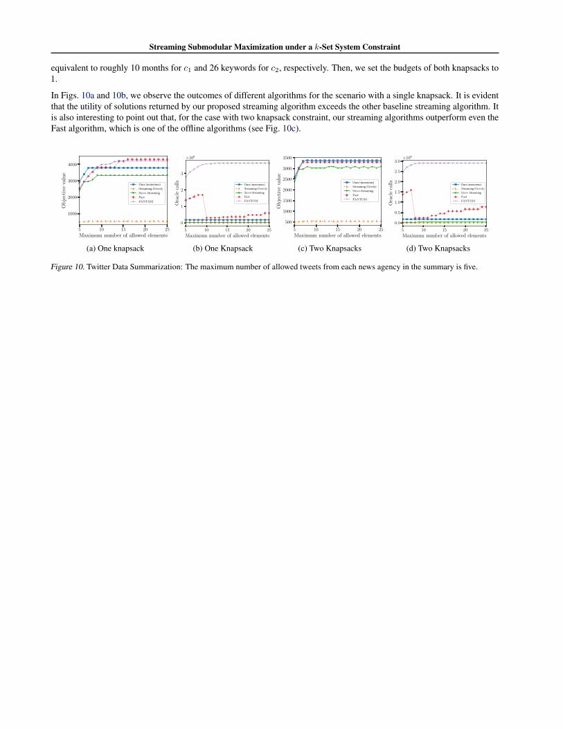
Streaming Submodular Maximization under a k-Set System Constraint
equivalent to roughly 10 months for c1 and 26 keywords for c2, respectively. Then, we set the budgets of both knapsacks to1.
In Figs. 10a and 10b, we observe the outcomes of different algorithms for the scenario with a single knapsack. It is evidentthat the utility of solutions returned by our proposed streaming algorithm exceeds the other baseline streaming algorithm. Itis also interesting to point out that, for the case with two knapsack constraint, our streaming algorithms outperform even theFast algorithm, which is one of the offline algorithms (see Fig. 10c).
5 10 15 20 25
Maximum number of allowed elements
1000
2000
3000
4000
Ob
ject
ive
valu
e
Ours (monotone)Streaming-Greedy Sieve-Streaming Fast FANTOM
(a) One knapsack
5 10 15 20 25
Maximum number of allowed elements
0
1
2
3O
racl
eca
lls
×106
Ours (monotone)Streaming-Greedy Sieve-Streaming Fast FANTOM
(b) One Knapsack
5 10 15 20 25
Maximum number of allowed elements
500
1000
1500
2000
2500
3000
3500
Ob
ject
ive
valu
e
Ours (monotone)Streaming-Greedy Sieve-Streaming Fast FANTOM
(c) Two Knapsacks
5 10 15 20 25
Maximum number of allowed elements
0.0
0.5
1.0
1.5
2.0
2.5
3.0
Ora
cle
call
s
×106
Ours (monotone)Streaming-Greedy Sieve-StreamingFast FANTOM
(d) Two Knapsacks
Figure 10. Twitter Data Summarization: The maximum number of allowed tweets from each news agency in the summary is five.