See discussions, stats, and author profiles for this publication at: https://www.researchgate.net/publication/264383076

Structural analysis with probability-boxes”, Int. J. Reliability and Safety, Vol.

6, Nos. 1/2/3, 2012.

Article · January 2012

CITATIONS

0

READS

119

1 author:

Some of the authors of this publication are also working on these related projects:

Interval FEA of thin plates View project

Interval Finite Element Approach for Inverse Problem Under Uncertainty View project

Rafi Muhanna

Georgia Institute of Technology

76 PUBLICATIONS 965 CITATIONS

SEE PROFILE

All content following this page was uploaded by Rafi Muhanna on 05 September 2014.

The user has requested enhancement of the downloaded file.

Int. J. Reliability and Safety, Vol. X, No. Y, XXXX

Copyright © 200X Inderscience Enterprises Ltd.

Structural analysis with probability-boxes

Hao Zhang* School of Civil Engineering, University of Sydney, NSW 2006, Australia Email: hao.zhang@sydney.edu *Corresponding author

Robert L. Mullen Department of Civil and Environmental Engineering, University of South Carolina, Columbia, SC 29208, USA Email: rlm@sc.edu

Rafi L. Muhanna School of Civil and Environmental Engineering, Georgia Institute of Technology, Savannah, GA 31407, USA Email: rafi.muhanna@gtsav.gatech.edu

Abstract: Probability-box (p-box) is a rigorous and practical way to represent epistemic sources of uncertainty where the available knowledge is insufficient to construct the required probability distributions. In this paper, interval finite element (FE) methods are combined with the concept of p-box to analyse structures subjected to uncertain loads modelled by p-boxes. Two methods, namely the discrete p-box convolution and interval Monte Carlo methods, are presented along with example problems. The computational efficiency of the p-box FE method is also presented.

Keywords: epistemic uncertainty; imprecise probability; interval analysis; interval finite element; Monte Carlo simulation; probability-box; p-box; random set; structural reliability.

Reference to this paper should be made as follows: Zhang, H., Mullen, R.L. and Muhanna R.L. (XXXX) ‘Structural analysis with probability-boxes’, Int. J. Reliability and Safety, Vol. X, No. Y, pp.xx–xx.

Biographical notes: [AQ1]

AQ1: Please supply brief career history of all the authors of not more than 100 words each.

H. Zhang, R.L. Mullen and R.L. Muhanna

1 Introduction

Engineering analysis and design require analysts to make assumptions at different levels. One of these levels is the choice of the mathematical model of the problem being analysed. Another level is the description of the model parameters. Assumptions and simplifications are made to facilitate processing the analysis and design, meaning that the validity of engineering computation is conditional on the priori assumptions. In a deterministic structural analysis, the loads and structural properties are assumed to have specific values. Conversely, if these assumptions do not hold, the uncertainties in the parameters have to be incorporated into the analysis process. The best candidate methods for handling uncertainties appear to be the methods of probability and statistics. Stochastic FE methods have been developed to analyse structures with random properties/loads (cf. Spanos, 1995). Probabilistic approaches require complete knowledge of the probability laws for the basic random variables. Samples of data available, however, might range from scarce or limited to comprehensive. When there is scarce data, analysts fall back to deterministic analysis, which is irrational and does not account for parameter variability. On the other hand, when more data are available but insufficient to distinguish between candidate probability functions, analysts supplement the available statistical data by judgmental information. The probabilistic analysis is thus subjective in nature. More advanced Bayesian methods provide a formal framework for combining judgmental information with observational data through Bayes’ theorem. Before receiving additional data, however, Bayesian approach remains a subjective representation of probability. In such a case, we find ourselves in the extreme either/or situation: a deterministic or a full probabilistic analysis. The former does not reflect parameter variabilities and the latter is conditional on the validity of the probability models describing the uncertainties. The above discussion illustrates the challenge that engineering analysis and design are facing in how to circumvent the situations that do not reflect the actual state of knowledge of considered systems and are based on unjustified assumptions.

Uncertainties can be classified in two general types, namely ‘aleatory’ and ‘epistemic’ (cf. Ferson and Ginzburg, 1996; Paté -Cornell, 1996; Ellingwood and Kinali, 2009; Helton et al., 2010). Aleatory uncertainty (also termed as irreducible uncertainty or stochastic uncertainty) refers to underlying, inherent variabilities of physical quantity (e.g. the variability in material strength). Aleatory uncertainty is generally quantified by a probability or frequency distribution. Epistemic uncertainty refers to uncertainty which results from lack of knowledge or incomplete information. In contrast with aleatory uncertainty, epistemic uncertainty may be reduced with additional data or information, or better modelling and better parameter estimation. Possible sources of epistemic uncertainties include modelling uncertainty and statistical uncertainty.

Structural analysis with probability-boxes

The distinction between aleatory and epistemic uncertainty is important when determining how each should be described mathematically. While probabilistic approach is widely accepted to represent aleatory uncertainty, the use of Bayesian approach for representation of epistemic uncertainty often raises debate. There is a perception that because epistemic uncertainty has a different nature, it cannot be fully characterised by probabilistic approaches (Elishakoff, 1995; Ferson and Ginzburg, 1996; Helton et al., 2010; Limbourg and de Rocquigny, 2010).

An increasingly popular and practical way to represent an imprecise probability function is to specify its lower and upper bounds. The mathematical frameworks using this methodology include Dempster–Shafer evidence theory (Dempster, 1967; Shafer, 1976), random set theory (Kendall, 1974), imprecise probability theory (Walley, 1991) and probability-box (p-box) (Ferson et al., 2003). These methods extend the traditional probability theory by allowing for intervals or sets of probabilities, and can handle the circumstances where analysts cannot specify (a) precise values for the statistical parameters (e.g. mean or variance) of the basic random variable; (b) the distribution shape for the basic random variables; or (c) the precise nature of dependencies between basic random variables, due to limited sample of data. These circumstances correspond to the common epistemic uncertainties encountered in engineering analysis.

P-boxes and Dempster–Shafer structures were employed to bound imprecisely specified probability distributions (see Ferson et al., 2003). The method was applied to environmental risk assessment (Tucker and Ferson, 2003). Tonon et al. (2006) considered the reliability analysis for an aircraft wing at the early stage of design process where the observational data are not point-valued but set-valued. Random sets were employed to represent the envelope of all probability distributions compatible with the available information. The limit state function was explicit and relatively simple (a linear function of independent random set variables). The Cartesian product method and interval arithmetic were used to propagate the random sets through the limit state function. Oberguggenberger and Fellin (2008) used random sets as a non-parametric means to describe the variability and uncertainty of input and response in geotechnical problems. Tchebycheff’s inequality was applied to the closed-form solution of First-Order Second-Moment (FOSM) method to approximate the mean and variance of response. Schweiger and Peschl (2005) used random sets to describe the uncertain material parameters in geotechnical engineering. Random sets were combined with FE method to perform a slope stability analysis and solve a deep excavation problem. The study used the vertex method to propagate the random set variables through the FE Analysis (FEA), assuming that the response quantity is strictly monotonic with respect to each random set variable. The monotonicity assumption, however, is difficult to verify for general structural mechanics problems (even for linear elastic problems). Zhang et al. (2010) considered structural reliability assessment when statistical parameters of probability functions cannot be determined precisely due to limited sample of data. Interval estimate of structural limit state probability was computed which provided a statement of confidence in the results of the reliability analysis.

In this work, we study structures subjected to uncertain loads modelled by imprecise probability functions. The response quantities (i.e. displacements) are determined implicitly by structural analysis. Two methods, namely the discrete p-box convolution and interval

H. Zhang, R.L. Mullen and R.L. Muhanna

Monte Carlo method, are employed to propagate the imprecise probability information through FE structural analysis. Numerical examples are given to demonstrate the two methods.

2 Finite element analysis with uncertain parameters

The numerical method most frequently used to capture the behaviour of complicated engineering systems appears to be the FEA. It provides numerical solution of the governing partial differential equations of field problems posed over a domain Ω. In FEA, this domain is replaced by the union ∪ of sub domains Ωe called finite elements. Elements are connected at points called nodes. The field quantity is locally (piecewise) approximated over each element by an interpolation formula expressed in terms of the nodal values of the field quantity. The assemblage of elements represents a discrete analogue of the original domain, and the associated system of algebraic equations represents a numerical analogue of the mathematical model of the problem being analysed. The solution for nodal quantities, when combined with the assumed field in any given element, completely determines the spatial variation of the field in that element. Many texts on FEA are available in the literature.

Numerically, a (displacement-based) linear static FEA yields a system of linear equations to be solved for displacements at nodes. i.e.

= ,Ku p (1)

where K is the structure stiffness matrix, u is the nodal displacement vector and p is the structure load vector. The structure stiffness matrix K is obtained as:

T

1,

eN

i i ii=

= ∑K L k L (2)

in which the matrix Li is referred to as element connectivity matrix, Ne is the number of elements and ki is the stiffness matrix of i-th element:

T d .ei V

Ω= ∫k B CB (3)

where B is the strain-displacement matrix, and C is the elasticity matrix. Equation (1) is solved for the nodal displacement u. Other responses, such as stresses, can be obtained from u.

Conceptually, an FEA can be expressed as :f →X Y , in which X is the vector of the basic parameters such as applied loads and material properties, Y is the vector of structural responses of interest and f is the mapping relating X and Y, determined implicitly by FEA. If (some of) the parameters X are uncertain, a non-deterministic FEA is required. Depending on the mathematical models of the uncertain parameters X, different non-deterministic FEA can be employed, such as stochastic FEA, fuzzy FEA, interval FEA and random set FEA. The connections between these non-deterministic FEA have been discussed by Muhanna et al. (2007b). Koyluoglu and Elishakoff (1998) made a comparison of stochastic FEA and interval FEA. In the present study, the uncertain parameters are modelled with p-boxes.

Structural analysis with probability-boxes

3 Arithmetic of p-boxes

Let F(x) denote the Cumulative Distribution Function (CDF) for a random variable X. When the probability function is imprecisely known, for any reference value x, an interval [ ( ), ( )]F x F x generally can be found to bound the possible values of F(x), i.e.

( ) ( ) ( ).F x F x F x≤ ≤ The bounds shall enclose all possible probabilities, and yet acceptably narrow to be useful. Such a pair of two CDFs ( )F x and ( )F x can be termed as ‘probability-bounds’ or ‘probability-box’ (p-box for short) (Ferson et al., 2003). Depending on the underlying sample space, a p-box may be discrete or continuous. P-box approach is closely related to other imprecise probability theories that induce lower and upper probability bounds to represent imprecise probability, such as random sets and Dempster–Shafer evidence. Their relationship has been discussed elsewhere (Alvarez, 2006; Baudrit et al., 2008).

Although p-box provides a concise representation of imprecise probability, propagation of p-boxes in complex engineering computations can be very challenging. In this work, the discrete p-box convolution and interval Monte Carlo method are used for computing with p-boxes.

3.1 Convolution of independent p-boxes

Williamson and Downs (1990) developed algorithms to compute binary arithmetic operations (addition, subtraction, multiplication and division) on pairs of independent discrete p-boxes. The algorithms are based on interval arithmetic (Moore, 1966) and Cartesian product method. Similar algorithms were also described by Berleant and collaborators in the context of automatically verified computations (Berleant, 1993; Berleant and Goodman-Strauss, 1998). These convolution algorithms were formalised later by Ferson et al. (2003).

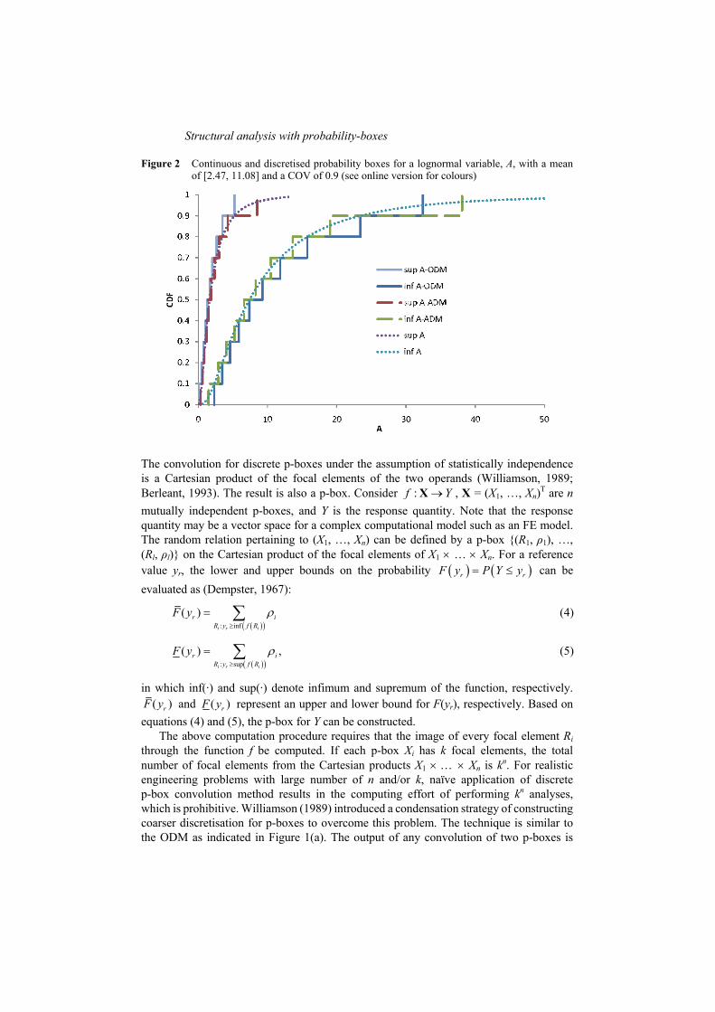
The convolution algorithms are based on discrete p-boxes. In computations involving continuous p-boxes, a discretisation procedure is necessary. A continuous p-box is approximated by a list of pairs (A1, m1), …, (Ai, mi), …, , in which Ai are intervals and mi are their associated probability masses. Ai can be termed as focal elements and mi can be viewed as the probability that Ai is the range of x (Dubois and Prade, 1991). Thus, a discrete p-box is analogous to a discrete probability distribution except that the probability mass is assigned to an interval rather than to a scalar value. Two discretisation methods have been proposed, namely the Outer Discretisation Method (ODM) (Williamson, 1989) and the Averaging Discretisation Method (ADM) (Tonon, 2004). The two methods are graphically demonstrated in Figures 1(a) and (b). In practice, unbounded distributions are truncated to a finite range when the ODM is selected. Clearly, the accuracy of the computation depends on the discretisation. The number of discretisation may need to be of the order 50–200, depending on the problem being solved. Take a log-normal random variable, A, for example. Consider a log-normal with an interval mean of [2.47, 11.08] and a Coefficient of Variation (COV) of 1.12. Figure 2 shows the continuous probability bounds and its ODM and ADM discretisation with ten focal elements of equal probability mass of 0.1. It should be noted that the discretisation can be non-uniform, i.e. a smaller probability mass can be used in the tail area (Kriegler, 2005). Since the log-normal is unbounded in the upper tail, the probability bounds for the ODM are truncated at a probability of 0.95. The use of ten focal elements in this

H. Zhang, R.L. Mullen and R.L. Muhanna

figure is for illustrative purposes and in practice, more focal elements would be used. It should also be emphasised that while the bounds of this p-box are defined by log-normal probability distributions, any CDF contained within the bounds, whether or not log-normal, is part of the p-box.

Figure 1 Descretisation of the probability-box: (a) outer descretisation method); (b) averaging descretisation method

(a)

(b)

Source: Tonon (2004)

Structural analysis with probability-boxes

Figure 2 Continuous and discretised probability boxes for a lognormal variable, A, with a mean of [2.47, 11.08] and a COV of 0.9 (see online version for colours)

The convolution for discrete p-boxes under the assumption of statistically independence is a Cartesian product of the focal elements of the two operands (Williamson, 1989; Berleant, 1993). The result is also a p-box. Consider :f Y→X , X = (X1, …, Xn)T are n mutually independent p-boxes, and Y is the response quantity. Note that the response quantity may be a vector space for a complex computational model such as an FE model. The random relation pertaining to (X1, …, Xn) can be defined by a p-box (R1, ρ1), …, (Rl, ρl) on the Cartesian product of the focal elements of X1 × … × Xn. For a reference value yr, the lower and upper bounds on the probability ( ) ( )r rF y P Y y= ≤ can be evaluated as (Dempster, 1967):

( )( ): inf

( )i r i

r iR y f R

F y ρ≥

= ∑ (4)

( )( ): sup

( ) ,i r i

r iR y f R

F y ρ≥

= ∑ (5)

in which inf(·) and sup(·) denote infimum and supremum of the function, respectively. ( )rF y and ( )rF y represent an upper and lower bound for F(yr), respectively. Based on

equations (4) and (5), the p-box for Y can be constructed. The above computation procedure requires that the image of every focal element Ri

through the function f be computed. If each p-box Xi has k focal elements, the total number of focal elements from the Cartesian products X1 × … × Xn is kn. For realistic engineering problems with large number of n and/or k, naïve application of discrete p-box convolution method results in the computing effort of performing kn analyses, which is prohibitive. Williamson (1989) introduced a condensation strategy of constructing coarser discretisation for p-boxes to overcome this problem. The technique is similar to the ODM as indicated in Figure 1(a). The output of any convolution of two p-boxes is

H. Zhang, R.L. Mullen and R.L. Muhanna

approximated by a p-box with N focal elements which conservatively enclose the original output. The resulting coarser p-box is used in the next step of calculation. Thus, the total number of function evaluation can be reduced to (n – 1)k2. Certainly, there is a trade-off between computational cost and accuracy of results. The condensation technique requires that the computation is performed in a sequence of binary operations. If a p-box structure occurs multiple times in the computation, the condensation algorithm treats the same p-box as independent p-boxes that happen to have the same bounds. This phenomenon, similar to the dependency problem in interval arithmetic (Moore, 1966; Neumaier, 1990), may introduce significant errors in the result. Because of the dependency problem, we limit our considerations to linear FEA with uncertainties only arising from the loads since the dependency problem can be eliminated in this case (Mullen and Muhanna, 1999).

3.2 Convolutions of p-boxes with any dependency

Williamson (1989) also addressed the convolutions of discrete p-boxes in the case where the two operands can have any dependency. The so-called dependency bounds (any dependency) can be calculated without constructing the entire Cartesian product. Let A and B are two discrete p-boxes, and each has n focal elements of equal probability mass of 1/n. Assume that the statistical dependence relationship between A and B is unknown. Consider C = A + B. The focal elements of C are given by

[ ] [ ] [ ]( ): ... 1inf 1 ,

j i nC i A j B i j n

−= + − + − (6)

[ ] [ ] [ ]( )0...

sup ,j i

C i A j B i j=

= + − (7)

where A[i] represents the interval bounds for the CDF with probability between i/n and (i + 1)/n. Each focal element of C has a probability mass of 1/n. Similar equations can be constructed for other arithmetic operators. Unlike the operations on independent variables, the dependency bounds do not require a condensation step and share the philosophy of the ODM. Obviously, the dependency bounds enclose the bounds based on the assumption of independence.

3.3 Interval Monte Carlo method

More recently, sampling methods were proposed to propagate p-boxes through probabilistic analysis (Alvarez, 2006; Zhang et al., 2010), Monte Carlo sampling methods are widely used for the purpose of computing statistics (i.e. moments, frequency distributions) of response variables for a complex system. Let X denote the vector of the basic random variables representing uncertain quantities such as applied loads, material strength and stiffness of a structure. Sample realisations ˆ

iX , i = 1, …, N, of X are randomly generated according to the joint probability density function of X. ˆ

iX are then fed into the FE model to compute the structural response ˆiy . Thus, a sample of structural response can be simulated, based on which the response statistics can be estimated. For instance, the mean of the response Y is estimated as:

1

1 ˆ .N

Y ij

yN

μ=

≈ ∑ (8)

Structural analysis with probability-boxes

For a reference value yr, the probability P[Y ≤ yr] is calculated from

[ ]1

1 ˆ ,N

j rj

P Y y I y yN =

⎡ ⎤≤ ≈ ≤⎣ ⎦∑ (9)

in which I[·] is the indicator function, having the value 1 if [·] is ‘true’ and the value 0 if [·] is ‘false’.

The above Monte Carlo sampling method can be extended to imprecise probability functions. When the basic variables X is modelled by imprecise probability functions having known bounds, the randomly sampled basic variables ˆ

iX vary in intervals. One can randomly generate such intervals using the inverse transform method (Ang and Tang, 1975).

Suppose an imprecise probability function is bounded by ( )F x and ( ),F x as shown in Figure 3. For each realisation to be generated, a standard uniform random number ui is first generated. The intersection of a line of ui and the lower and upper bounds defining the imprecise CDF will result in an interval [ , ].i ix x The method is graphically demonstrated in Figure 3 for one-dimensional case.

1 1( ), ( ).i i i ix F u x F u− −= = (10)

Such a pair of ix and ix form an interval [ , ]i ix x which contains ‘all possible’ simulated numbers from the ensemble of distributions for a particular ui.

Figure 3 Generation of random intervals from a p-box

The randomly generated interval values for the basic variables are then entered into the FE model. Conceivably, the resulting structural response ˆiy itself varies in a range. If the range (minimum and the maximum) of ˆiy can be computed, it becomes straightforward to compute the bounds for P[Y ≤ yr]:

( ) [ ]1 1

1 1ˆ ˆmax [min( ) ].N N

j r r j rj j

I y y P Y y I y yN N= =

⎡ ⎤≤ ≤ ≤ ≤ ≤⎣ ⎦∑ ∑ (11)

H. Zhang, R.L. Mullen and R.L. Muhanna

Therefore, plot two cumulative frequency distributions, one for min 1ˆ( )y , …, min ˆ( )Ny , and the other for max 1ˆ( )y , …, max ˆ( )Ny . The obtained two frequency distributions represent the probability bounds for the structural response Y. Based on the p-box of Y, reliability assessment or risk analysis can be performed (Zhang et al., 2010).

4 Computing the ranges of structural responses: interval FEA

Discrete p-box convolution and interval Monte Carlo method both require computing the range (max. and min.) of structural responses when the basic variables vary in intervals. This can be formulated as an interval FEA problem. Computing the exact range of structural response, however, is NP-hard even for linear static problems. In practice, a feasible solution is to seek reasonably accurate outer bounds for the response range. The bounds should be rigorous and accurate, i.e. they guarantee to enclose the exact range of the response, but not excessively conservative. Since multiple interval FE analyses are required (e.g. 1000 analyses in the interval Monte Carlo method), it is critical to perform the interval FEA efficiently.

A variety of solution techniques have been proposed for the interval FEA, including the combinatorial method (Ganzerli and Pantelides, 1999), perturbation method (McWilliam, 2000), sensitivity analysis method (Pownuk, 2004), optimisation method (Möller and Beer, 2004) and direct interval arithmetic method (Mullen and Muhanna, 1999; Dessombz et al., 2001; Muhanna and Mullen, 2001). Zhang (2005) and Moens and Vandepitte (2005) reviewed various interval FE solutions.

In this paper, the interval FEA is solved using the direct interval arithmetic method. Linear interval system equation is formulated using an element-by-element procedure, and solved by modified interval fixed point iteration. The advantage of the method is that it does not rely on the monotonicity assumption of the response quantities, and provide a guaranteed, yet acceptably narrow enclosure (outer bound) for the interval FE response quantities. Details of the methods can be found elsewhere (Muhanna et al., 2005, Zhang, 2005; Muhanna et al., 2007a).

5 Examples

5.1 Illustrative example

The first example is to illustrate the basic concepts of discrete p-boxes computation and interval sampling method. Consider A to be the log-normal in Figure 2 with a mean of [2.47, 11.08] and a COV of 0.9. B is bounded by normal distributions with a mean of [4, 5.5] and a standard deviation of 1.5. In selecting bounding distributions one must use a point value for COV in log-normal distribution and a point value for variance in a normal distribution to prevent the bounds from crossing. We will first assume that A and B are statistically independent. We now examine the addition of A + B = C.

The discrete p-box computation method is used first. For simplicity, each of the two bounding CDFs is discretised into 10 intervals with equal probability mass of 0.1. The discretisation for A and B is shown in Figure 2 and Figure 4, respectively. Figure 4 shows both the ODM and ADM discretisation approaches. The unbounded CDF for B was

Structural analysis with probability-boxes

truncated at a probability of 0.05 and 0.95 at the two tails for the ODM and while the distribution is unbounded, the integrated average values used in the ADM method are finite. The addition of A and B under the assumption of independence is calculated by constructing a Cartesian product of each interval in A and B as shown in Table 1 for the ODM. The first row and column of the table gives the interval focal elements for A and B, respectively. Ai and Bi denote the i-th focal elements. The cells inside the table form the Cartesian product of A and B. Each of the resulting 100 intervals has a probability mass of 0.01 (0.1 × 0.1). The lower and upper bounds of the 100 intervals are then sorted in ascending order, and the p-box for C is constructed as shown in Figure 5.

Figure 4 Discretised probability boxes for a normal variable, B, with a mean of [4, 5.5] and a standard deviation of 1.5 (see online version for colours)

Figure 5 The sum of A and B. Comparison of interval Monte Carlo result, and ODM results with/without condensation (see online version for colours)

H. Zhang, R.L. Mullen and R.L. Muhanna

Note that while A and B each has 10 interval focal elements, the number of focal elements in A + B calculated from the Cartesian product increases to 100. Thus, the naïve use of discrete p-boxes after a few operations will lead to a computationally unfeasible result when operating on independent quantities. The condensation strategy developed by Williamson (1989) can be employed to ‘compress’ the 100 interval focal elements in A + B back to a 10 interval discretisation for subsequence operations. The condensation is accomplished by grouping the sorted bounds into groups of n (n = 10 in this example) and replacing the n intervals with a single interval whose lower bound is the lower bound of the first interval in the group and whose upper bound is the upper bound of the last interval in the group. Williamson’s method follows the philosophy of the ODM ensuring that the condensed p-box contains all the possible CDFs in the condensed structure. One can also compress a p-box following the philosophy of constructing the best-fit course discretisation of the p-box by using the ADM. In this compression, every group of n intervals are replaced by a single interval consisting of the average of the n upper and lower bounds. The ODM condensed A + B is also shown in Figure 5 to compare with the original result.

The interval sampling method was used next. Hundred interval samples of A and B were generated. For each pair of sampled ˆ

iA and ˆ ,iB their addition was computed. The interval Monte Carlo sampling results are also shown in Figures 5 and 6 for comparison to the p-box results. Table 1 Interval focal element for A + B

[ ] [ ] [ ] [ ]1 2 9 10: 0.51,3.58 : 2.08,4.24 : 5.26,7.43 : 5.92,8.99A A A A…

[ ][ ][ ]

[ ][ ]

1

2

3

9

10

: 0,2.33: 0.52,3.46: 0.77,4.61

: 3.52,23.4: 5.22,60

BBB

BB

[ ] [ ] [ ] [ ][ ] [ ] [ ] [ ][ ] [ ] [ ] [ ]

[ ] [ ] [ ] [ ][ ] [ ] [ ] [ ]

0.51,5.91 2.08,6.57 5.26,9.76 5.92,11.321.03,7.04 2.6,7.7 5.78,10.89 6.44,12.451.28,8.19 2.85,8.85 6.03,12.04 6.69,13.6

4.03,26.98 5.6,27.64 8.78,30.83 9.44,32.395.73,63.58 7.3,64.24 10.48,67.4 11.44,68.9

………

……

The computed bounds on A + B are dependent on the discretisation methods used. In Figure 6, the solution of A + B is computed by ODM and ADM. Except in the tails of the distribution, the ADM is enclosed by the ODM results. The narrower values of the ODM in the tails of the distribution are due to the truncation of the bounding CDF. Changes in the truncation point will change the relative bounding values at the tails of the CDF. The ODM method also bounds the Monte Carlo solution except at the tails of the distributions. The ADM method follows the Monte Carlo values along the entire distribution.

One way to evaluate the discretisation errors introduced by the discrete p-box method is to calculate the bounds on the mean value of A + B. It should be noted that the exact mean of A + B is [6.47, 16.58] (the sum of the means of A and B). The interval means of A + B obtained from various discretisation methods are given in Table 2.

Structural analysis with probability-boxes

Figure 6 The sum of A and B. Comparison of interval Monte Carlo result, and ODM and ADM results, dependency bound (see online version for colours)

Table 2 Mean values of C = A + B using various methods

Method Condensed Truncated Mean Exact* No No [6.47, 16.58] ODM* No Yes [5.63, 17.39] ADM* No Yes [6.22, 15.41] ADM* No No [6.45, 16.48] ODM* Yes Yes [5.22, 18.64] ADM* Yes Yes [6.22, 15.41] ADM* Yes No [6.45,16.48] Dependency bounds No Yes [3.90, 19.61] IMC 500* No No [6.43, 16.40]

Note: * Assume A and B are independent; IMC 500 = 500 interval Monte Carlo sampling.

The solutions with the best calculation of the bounds of the mean are obtained by the ADM and interval Monte Carlo methods. We attribute this to the lack of the need to truncate an unbounded distribution and that the condensation operation in the ADM method preserves the mean value of the p-box. The impact of truncation can be seen by comparing the ADM method using truncated distributions with the full unbounded distributions. The truncated distribution decreases the bounds on the mean since the log-normal distribution is truncated only on the upper tail while the normal distribution was truncated symmetrically. In the case of ODM, the condensation operation results in an increase of the width of the mean after condensation. This overestimation is due to the outward bounding of the condensed p-box and is indicative of a continually increasing discretisation error associated with the ODM method.

H. Zhang, R.L. Mullen and R.L. Muhanna

The dependency bounds are the widest of the calculated bounds. This is not surprising since the ODM method is used and the bounds are required to contain the manifold of all possible dependency between the variables. Our observation is that unlike the addition of independent variables, the bounds themselves are not a possible CDF solution.

5.2 Truss structure

The second example is a linear elastic planar truss bridge, shown in Figure 7. Its reliability has been studied by Zhang et al. (2010). The structural response of interest is the vertical deflection at node 5, u5, under the applied three loads. The cross-sectional areas for elements 1–6 is 10.32 cm2 and for elements 7–15 the cross-sectional area is 6.45 cm2. The elastic modulus for all elements is 200 GPa. The loads are identified as the basic random variables, and modelled by log-normal distributions. The sample statistics for the loads are presented in the second and third columns of Table 3. Assume that the statistics were obtained from 20 samples, and the (population) standard deviations are equal to those obtained from the samples. The logarithmic mean of the loads is considered to be interval due to the limited sample size. Let λi denote the mean of Ln Pi. In the classical statistical framework, the confidence intervals for λi can be easily computed (cf. Ang and Tang, 1975). The last column of Table 3 gives the 90% confidence intervals for λi, which are used as the interval estimates for λi in the subsequent calculations. Therefore, the loads are represented by p-boxes defined by log-normal distributions with interval means. Two cases are considered: (a) the three loads are mutually independent, and (b) the loads can have any possible dependency. Table 3 Statistics for the loads (unit: kN)

Variables Sample mean Stand. Dev. Interval mean1 Ln P1 4.483 0.09975 [4.4465, 4.5199] Ln P2 5.582 0.09975 [5.5452, 5.6186] Ln P3 4.483 0.09975 [4.4465, 4.5199]

Note: 1 90% confidence interval.

Figure 7 Truss structure

Structural analysis with probability-boxes

5.2.1 Case 1: loads are independent

For Case 1, both interval Monte Carlo and discrete p-box methods are used. In the latter, the CDF of each load is discretised into n uniform levels. The inverse transformation of the bounding CDF is used to construct the interval bounds for each discrete probability level. Using the arithmetic of discrete p-boxes, the nodal displacements are then calculated using equation (12):

u = K−1p. (12)

Since in this example the stiffness (K) of the structure is constant and only the loads, P, involve random variables, the displacements become a linear function of the random loads. Thus, the statistical moments for u can be easily computed as calculating the moments of linear functions of random variables (Ang and Tang, 1975). Let μu5 denote the mean of u5. The exact bounds for μu5 are computed as [−6.1625,−5.7264] (cm), in which the minus sign indicates the displacement is downwards. This result is used to validate the discrete p-box method and the interval Monte Carlo method. Table 4 compares the exact bounds for μu5 and those computed from the interval Monte Carlo method with different number of simulations, and from both ODM and ADM discrete p-box computations with different number of discretisations. In discrete p-box methods, the same number of discretisations is used for all three loads. Because the log-normal is unbounded in the upper tail, its CDF was truncated at a probability of 0.999 in the p-box discretisations. The exact result is chosen as a reference, and the relative errors of other solutions are listed in the table. In Table 4, ‘IMC n’ refers to the interval Monte Carlo method with n samples, and ‘p-box n’ refers to the discrete p-box calculation with n discretisations. It can be seen that the interval Monte Carlo results match well with the exact solution. Even for a relatively small number of simulations (500 simulations), the relative errors for the computed bounds are around 1%. The discrete p-box method also yields reasonable results, with relative errors around 1.5% if 100 ODM discretisations were used, while it is 0.8% for ADM. As expected, the results become more accurate as the number of discretisations increases.

Table 4 Bounds for μu5 computed by the interval Monte Carlo method and discrete p-box calculation, Case 1 (unit: cm)

Method Lower bound Error Upper bound Error IMC 500 −6.2313 1.12% −5.7623 0.63% IMC 5,000 −6.2253 1.02% −5.7568 0.53% IMC 50,000 −6.2235 1.0% −5.7551 0.50% IMC 250,000 −6.2239 1.0% −5.7555 0.51% p-box ODM 50 −6.2971 2.18% −5.5293 3.44% p-box ODM 100 −6.2432 1.31% −5.6385 1.53% p-box ODM 200 −6.2197 0.93% −5.6952 0.54% p-box ADM 50 −6.2332 1.15% −5.6362 1.58% p-box ADM 100 −6.2120 0.80% −5.6952 0.55% p-box ADM 200 −6.2029 0.66% −5.7249 0.03% Exact solution: [−6.1625, −5.7264]

H. Zhang, R.L. Mullen and R.L. Muhanna

In addition to the mean value, bounds on any percentile value of the response quantity can be readily obtained based on equation (11). Table 5 presents the bounds for the 95 percentile values for u5 computed from interval Monte Carlo method. Figure 8 plots the p-box for u5 obtained from the interval Monte Carlo method with 50,000 samples, as well as the result from the discrete ODM p-box computations using 200 interval discretisations for each load. As can be seen in the figure, the two distribution bounds almost overlap except at the tails where the Monte Carlo results are inside the discrete p-box results. This shows that ODM p-box computations provide guaranteed bounds.

Figure 8 Probability bounds for u5, Case 1 (see online version for colours)

Table 5 95 percentile for u5 computed by the interval Monte Carlo method and discrete p-box calculation, Case 1 (unit: cm)

Methods Lower bound Upper bound IMC 500 −6.9408 −6.4218 IMC 5,000 −6.9872 −6.4649 IMC 50,000 −6.9988 −6.4744 IMC 250,000 −7.0065 −6.4817

5.2.2 Case 2: loads with any possible dependency

In Case 2, an assumption of any possible dependency between the three loads was made. It must be noted that the commonly used ‘coefficient of correlation’ (Pearson’s correlation coefficient) represents only linear dependencies between the variables. The dependence relationship considered here is not limited to the linear dependence but also includes all higher order dependency. The interval Monte Carlo method can handle the random variables with interval coefficient of correlation (interval linear dependency) (Zhang and Reid, 2010). However, to the best knowledge of the authors, the application of interval Monte Carlo method in solving unknown higher order dependency is still under investigation. Thus, only the discrete p-box method was employed to solve Case 2.

Structural analysis with probability-boxes

The bounds on the cumulative distribution functions for u5 for Cases 1 and 2 are compared in Figure 9. It is clear that the assumption of any dependency of the loading results in much wider bounds on the possible CDF. The comparison highlights the effect of the dependency of the loads on the results.

Figure 9 Probability bounds for u5, Case 2 (see online version for colours)

5.2.3 Comparison of computational efficiency

Table 6 compares the computational time for the interval Monte Carlo method (for the independent case) and the discrete p-box calculations for both cases. All computations were carried out on a PC with an Intel CoreTM2 Duo T7250 @2.0 GHz CPU with a single thread program. The comparisons are illustrative only and no claim to an optimised implementation is made. Table 6 Computational CPU time (seconds) for the interval Monte Carlo method and discrete

p-box method

Method CPU time IMC 50,000 17 IMC 500,000 180 p-box 100 independent ODM 13 p-box 100 dependency 1 p-box 200 independent ODM 99 p-box 200 dependency 3

6 Conclusion

P-box method is applied in structural mechanics problem to model uncertain loads. Two approaches have been introduced, namely interval Monte Carlo and discrete p-box method to propagate p-boxes through FE analyses. In the discrete p-box convolution, two

H. Zhang, R.L. Mullen and R.L. Muhanna

discretisation methods have been used: ODM and ADM. The ODM method provides guaranteed bounds while the ADM provides a smaller discretisation error with the loss of guaranteed bounds. The ADM discrete p-box and interval Monte Carlo have comparable computational cost for similar level of accuracy, with the interval Monte Carlo preferred when a smaller number of simulations are used. The ADM and interval Monte Carlo do not provide guaranteed bounds on the solution. Only discrete p-box convolution method can handle the case when the dependency between random loads is not known.

References Alvarez, D.A. (2006) ‘On the calculation of the bounds of probability of events using infinite

random sets’, International Journal of Approximate Reasoning, Vol. 43, pp.241–267. Ang, A.H-S. and Tang, W. (1975) Probability Concepts in Engineering Planning and Design

(Vol. 1-Basic Principles), John Wiley, New York. Baudrit, C., Dubois, D. and Perrot, N. (2008) ‘Representing parametric probabilistic models tainted

with imprecision’, Fuzzy Sets and Systems, Vol. 159, pp.1913–1928. Berleant, D. (1993) ‘Automatically verified reasoning with both intervals and probability density

functions’, Interval Computations, Vol. 2, pp.48–70. Berleant, D. and Goodman-Strauss, C. (1998) ‘Bounding the results of arithmetic operations on

random variables of unknown dependency using intervals’, Reliable Computing, Vol. 4, No. 2, pp.147–165.

Dempster, A.P. (1967) ‘Upper and lower probabilities induced by a multivalued mapping’, Annals of Mathematical Statistics, Vol. 38, pp.325–339.

Dessombz, O., Thouverez, F., Laîné, J-P. and Jézéquel, L. (2001) ‘Analysis of mechanical systems using interval computations applied to finite elements methods’, Journal of Sound and Vibration, Vol. 238, No. 5, pp.949–968.

Dubois, D. and Prade, H. (1991) ‘Random sets and fuzzy interval analysis’, Fuzzy Sets of Systems, Vol. 42, pp.87–101.

Elishakoff, I. (1995) ‘Essay on uncertainties in elastic and viscoelastic structures: from A.M. Freudenthal’s criticisms to modern convex modeling’, Computers & Structures, Vol. 56, No. 6, pp.871–895.

Ellingwood, B.R. and Kinali, K. (2009) ‘Quantifying and communicating uncertainty in seismic risk assessment’, Structural Safety, Vol. 31, pp.179–187.

Ferson, S. and Ginzburg, L.R. (1996) ‘Different methods are needed to propagate ignorance and variability’, Reliability Engineering System Safety, Vol. 54, Nos. 2/3, pp.133–144.

Ferson, S., Kreinovich, V., Ginzburg, L., Myers, D.S. and Sentz, K. (2003) Constructing Probability Boxes and Dempster-Shafer Structures, Technical Report SAND2002-4015, Sandia National Laboratories.

Ganzerli, S. and Pantelides, C.P. (1999) ‘Load and resistance convex models for optimum design’, Journal of Structural Optimization, Vol. 17, pp.259–268.

Helton, J.C., Johnson, J.D., Oberkampf, W.L. and Sallaberry, C.J. (2010) ‘Representation of analysis results involving aleatory and epistemic uncertainty’, International Journal of General Systems, Vol. 39, No. 6, pp.605–646.

Kendall, D.G. (1974) ‘Foundations of a theory of random sets’, in Harding, E. and Kendall, D. (Eds): Stochastic Geometry, Wiley, New York, pp.322–376.

Koyluoglu, H.U. and Elishakoff, I. (1998) ‘A comparison of stochastic and interval finite elements applied to shear frames with uncertain stiffness properties’, Computers & Structures, Vol. 67, Nos. 1–3, pp.91–98.

Kriegler, E. (2005) Imprecise Probability Analysis for Integrated Assessment of Climate Change, PhD Thesis, Universität Potsdam, Germany.

Structural analysis with probability-boxes

Limbourg, P. and de Rocquigny, E. (2010) ‘Uncertainty analysis using evidence theory – confronting level-1 and level-2 approaches with data availability and computational constraints’, Reliability Engineering & System Safety, Vol. 95, No. 5, pp.550–564.

McWilliam, S. (2000) ‘Anti-optimisation of uncertain structures using interval analysis’, Computers & Structures, Vol. 79, pp.421–430.

Moens, D. and Vandepitte, D. (2005) ‘A survey of non-probabilistic uncertainty treatment in finite element analysis’, Computer Methods in Applied Mechanics and Engineering, Vol. 194, Nos. 12–16, pp.1527–1555.

Möller, B. and Beer, M. (2004) Fuzzy-Randomness-Uncertainty in Civil Engineering and Computational Mechanics, Springer-Verlag, Berlin and Heidelberg.

Moore, R.E. (1966) Interval Analysis, Prentice-Hall Inc., Englewood Cliffs, NJ. Muhanna, R.L. and Mullen, R.L. (2001) ‘Uncertainty in mechanics problems – interval-based

approach’, Journal of Engineering Mechanics, Vol. 127, No. 6, pp.557–566. Muhanna, R.L., Mullen, R.L. and Zhang, H. (2005) ‘Penalty-based solution for the interval finite

element methods’, Journal of Engineering Mechanics, Vol. 131, No. 10, pp.1102–1111. Muhanna, R.L., Zhang, H. and Mullen, R.L. (2007a) ‘Combined axial and bending stiffness

in interval finite-element methods’, Journal of Structural Engineering, 133, Vol. 12, pp.1700–1709.

Muhanna, R.L., Zhang, H. and Mullen, R.L. (2007b) ‘Interval finite element as a basis for generalized models of uncertainty in engineering mechanics’, Reliable Computing, Vol. 13, No. 2, pp.173–194.

Mullen, R.L. and Muhanna, R.L. (1999) ‘Bounds of structural response for all possible loadings’, Journal of Structural Engineering, Vol. 125, No. 1, pp.98–106.

Neumaier, A. (1990) Interval Methods for Systems of Equations, Cambridge University Press, Cambridge.

Oberguggenberger, M. and Fellin, W. (2008) ‘Reliability bounds through random sets: non-parametric methods and geotechnical applications’, Computers & Structures, Vol. 86, No. 10, pp.1093–1101.

Paté-Cornell, M.E. (1996) ‘Uncertainties in risk analysis: six levels of treatment’, Reliability Engineering & System Safety, Vol. 54, Nos. 2/3, pp.95–111.

Pownuk, A. (2004) ‘Efficient method of solution of large scale engineering problems with interval parameters’, in Muhanna, R.L. and Mullen, R.L. (Eds): Proceedings of the NSF Workshop on Reliable Engineering Computing, 15–17 September, Savannah, GA.

Schweiger, H.F. and Peschl, G.M. (2005) ‘Reliability analysis in geotechnics with the random set finite element method’, Computers and Geotechnics, Vol. 32, No. 6, pp.422–435.

Shafer, G. (1976) A Mathematical Theory of Evidence, Princeton University Press, Princeton, NJ. Spanos, P.D. (Ed.) (1995) Computational Stochastic Mechanics, Balkema, Rotterdam. Tonon, F. (2004) ‘Using random set theory to propagate epistemic uncertainty through a

mechanical system’, Reliability Engineering & System Safety, Vol. 85, pp.169–181. Tonon, F., Bae, H-R., Grandhi, R. and Pettit, C. (2006) ‘Using random set theory to calculate

reliability bounds for a wing structure’, Structure and Infrastructure Engineering, Vol. 2, Nos. 3/4, pp.191–200.

Tucker, W.T. and Ferson, S. (2003) ‘Probability bounds analysis in environmental risk assessment’, Applied Biomathematics, Setauket, New York.

Walley, P. (1991) Statistical Reasoning with Imprecise Probabilities, Chapman and Hall, London. Williamson, R. (1989) Probabilistic Arithmetic, PhD Thesis, University of Queensland, Australia. Williamson, R. and Downs, T. (1990) ‘Probabilistic arithmetic I: numerical methods for calculating

convolutions and dependency bounds’, International Journal of Approximate Reasoning, Vol. 4, No. 2, pp.89–158.

H. Zhang, R.L. Mullen and R.L. Muhanna

Zhang, H. (2005) Nondeterministic Linear Static Finite Element Analysis: An Interval Approach, PhD Thesis, Georgia Institute of Technology, USA.

Zhang, H., Mullen, R.L. and Muhanna, R.L. (2010) ‘Interval Monte Carlo methods for structural reliability’, Structural Safety, Vol. 32, No. 3, pp.183–190.

Zhang, H. and Reid, S. (2010) ‘Comparison of methods for structural reliability assessment under parameter uncertainties’, in Li, J., Zhao, Y-G., Chen, J. and Peng, Y. (Eds): Proceedings of the International Symposium on Reliability Engineering and Risk Management (ISRERM2010), 23–26 September, Tongji University Press, Shanghai, China.

View publication statsView publication stats