Structural Macroeconometrics

Chapter 9. Bayesian Methods

David N. DeJong Chetan Dave

1 Overview of Objectives

Chapter 8 demonstrated use of the Kalman �lter for evaluating the likelihood function

associated with a given state-space representation. It then described the pursuit of empirical

objectives using classical estimation methods. This chapter characterizes and demonstrates

an alternative approach to this pursuit: the use of Bayesian methods.

A distinct advantage in using structural models to conduct empirical research is that

a priori guidance concerning their parameterization is often much more readily available

than is the case in working with reduced-form speci�cations. The adoption of a Bayesian

statistical perspective in this context is therefore particularly attractive, as it facilitates the

formal incorporation of prior information in a straightforward manner.

The reason for this is that from a Bayesian perspective, parameters are interpreted as

random variables. In the estimation stage, the objective is to make conditional probabilistic

statements regarding the parameterization of the model. Conditioning is made with respect

to three factors: the structure of the model; the observed data; and a prior distribution

speci�ed for the parameters. The structure of the model and the observed data combine to

form a likelihood function. Coupling the likelihood function with a prior distribution using

Bayes�Rule yields an associated posterior distribution.

Note that under the Bayesian perspective, both the likelihood function and posterior

distribution can be used to assess the relative plausibility of alternative parameterizations of

the model. Use of the likelihood function for this purpose gives exclusive voice to the data;

use of the posterior distribution gives voice to both the data and the researcher. The point

of this observation is that the incorporation of prior information is not what distinguishes

1

classical from Bayesian analysis: the distinguishing feature is the probabilistic interpretation

assigned to parameters under the Bayesian perspective.

So, it is not necessary to go about specifying prior distributions to gain distinction as

a Bayesian. But as noted, in the context of working with structural models the ability

to do so is often advantageous. Indeed, one interpretation of a calibration exercise is of a

Bayesian analysis involving the speci�cation of a point-mass prior over model parameters.

The incorporation of prior uncertainty into such an analysis through the speci�cation of

a di¤use prior gives voice to the data regarding model parameterization, and in so doing

enables the formal pursuit of a wide range of empirical objectives.

Broadly de�ned, Bayesian procedures have been applied to the analysis of DSGEs in

pursuit of three distinct empirical objectives; all three are discussed and demonstrated in this

chapter. First, they have been used to implement DSGEs as a source of prior information

regarding the parameterization of reduced-form models. An important goal in this sort

of exercise is to help provide theoretical context for interpreting forecasts generated by

popular reduced-form models, most notably vector autoregressions (VARs). Second, they

have been used to facilitate the direct estimation of DSGEs, and to implement estimated

models in pursuit of a variety of empirical objectives. A leading objective has been the

indirect measurement of unobservable facets of macroeconomic activity (e.g., time-series

observations of productivity shocks, time spent outside the labor force on home-production

and skill-acquisition activities, etc.). Third, Bayesian procedures have been used to facilitate

model comparisons. As an alternative to the classical hypothesis-testing methodology, in the

Bayesian context model comparison is facilitated via posterior odds analysis. Posterior odds

convey relative probabilities assigned to competing models, calculated conditionally given

2

priors and data. They are straightforward to compute and interpret even in cases where all

competing models are known to be false, and when alternatives are non-nested.

The analyses described in this chapter entail the use of computationally intensive numer-

ical integration procedures, and there are many alternative procedures available for facilitat-

ing their implementation. We have sought to keep this chapter relatively user friendly: the

numerical methods presented here were chosen with this objective in mind. Guidance for

readers interested in exploring alternative procedures is provided throughout the chapter.

Overviews of numerical methods are provided by Geweke (1999a) and Robert and Casella

(1999). In addition, Koop (2003) provides a general overview of Bayesian statistical meth-

ods with an eye towards discussing computational issues. Finally, Bauwens, Lubrano and

Richard (1999) provide a computationally based overview of the application of Bayesian

methods to the study of a broad range of dynamic reduced-form models.

2 Preliminaries

Likelihood functions provide the foundation for both classical and Bayesian approaches

to statistical inference. To establish the notation used throughout this chapter, let us brie�y

re-establish their derivation. We begin with a given structural model A with parameters

collected in the vector �. Log-linearization of the model yields a state-space representation

with parameters collected in the vector �(�). Coupled with a distributional assumption

regarding the disturbances included in the model, the state-space representation yields an

associated likelihood function, which can be evaluated using the Kalman �lter. Letting X

denote the sample of observations on the observed variables in the system, the likelihood

3

function is written as L(Xj�;A). Note that the mapping from � to � is taken for granted

under this notation: this is because � typically serves as the primary focus of the analysis.

When working only with a single model, the dependence of the likelihood function on A will

also be taken for granted, and the function will be written as L(Xj�).

From a classical perspective, parameters are interpreted as �xed but unknown entities,

and the likelihood function is interpreted as a sampling distribution for the data. The

realization of X is thus interpreted as one of many possible realizations from L(Xj�) that

could have been obtained. Inferences regarding the speci�cation of � center on statements

regarding probabilities associated with the particular observation of X for given values of �.

From a Bayesian perspective, the observation of X is taken as given, and inferences re-

garding the speci�cation of � center on statements regarding probabilities associated with

alternative speci�cations of � conditional on X. This probabilistic interpretation of � gives

rise to a potential avenue for the formal incorporation of a priori views regarding its spec-

i�cation. This is facilitated via the speci�cation of a prior distribution for �, denoted as

�(�).

To motivate the incorporation of �(�) into the analysis, recall the de�nition of conditional

probability, which holds that the joint probability of (X;�) may be calculated as

p(X;�) = L(Xj�)�(�); (1)

or reversing the roles of � and X,

p(X;�) = P (�jX)p(X): (2)

4

In (1) the likelihood function is used to perform the conditional probability calculation,

and conditioning is made with respect to �; �(�) in turn assigns probabilities to speci�c

values of �: In (2), P (�jX) is used to perform the conditional probability calculation, and

conditioning is made with respect to X; p(X) in turn assigns probabilities to speci�c values

of X. Eliminating p(X;�) by equating (1) and (2) and solving for P (�jX) yields Bayes�

Rule:

P (�jX) =L(Xj�)�(�)p(X)

(3)

/ L(Xj�)�(�);

where p(X) is a constant from the point of view of the distribution for �.

P (�jX) in (3) is the posterior distribution. Conditional onX and the prior �(�), it assigns

probabilities to alternative values of �; this distribution is the central focus of Bayesian

analyses.

The typical objective of a Bayesian analysis involves the calculation of the conditional

expected value of a function of the parameters g(�):1

E [g(�)] =

Rg(�)P (�jX)d�RP (�jX)d� : (4)

This objective covers a broad range of cases, depending upon the speci�cation of g(�). For

example, if g(�) is simply the identity function, then (4) delivers the posterior mean of �.

Alternatively, if g(�) is an indicator over a small interval for �j, the jth element of � (e.g.,

1The denominator is included in (4) to cover the general case in which p(X) in (3) is unknown, and thusP (�jX) does not integrate to 1.

5

g(�) = 1 for �j 2 [�j �j), and 0 otherwise), then assigning indicators over the support of

each element of � would enable the construction of marginal predictive density functions

(p.d.f.s) for each structural parameter of the underlying model.2 Further elaboration for

this important example is provided below in this section. Marginal p.d.f.s for additional

functions such as spectra, impulse response functions, predictive densities, and time-series

observations of unobservable variables included in the structural model may be constructed

analogously. Whatever the speci�cation of g(�) may be, (4) has a standard interpretation:

E [g(�)] is the weighted average of g(�), with the weight assigned to a particular value of �

determined jointly by the data (through the likelihood function) and the prior.

As noted, numerical integration procedures feature prominently in Bayesian analyses.

This is due to the fact that in general, it is not possible to calculate E [g(�)] analytically.

Instead, numerical methods are used to approximate the integrals that appear in (4).

In the simplest case, it is possible to simulate random drawings of � directly using the

posterior distribution P (�jX). In this case, (4) may be approximated via direct Monte Carlo

integration.3 Let �i denote the ith of a sequence of N draws obtained from P (�jX). Then

by the law of large numbers (e.g., as in Geweke, 1989):

gN =

�1

N

� NXi=1

g(�i)! E [g(�)] ; (5)

where! indicates convergence in probability. The numerical standard error associated with

2Referring to the p.d.f. of �j ; the term marginal indicates that the p.d.f. is unconditional on the valuesof the additional elements of �:

3Rubinstein (1981) describes algorithms for obtaining simulated realizations from a wide range of p.d.f.s.Monte Carlo methods were introduced in the economics literature by Kloek and van Dijk (1978).

6

gN is 1=pN times the standard deviation of g(�):

s:e:(gN) =�(g(�))p

N: (6)

De�ning �N(g(�)) as the sample standard deviation of g(�),

�N(g(�)) =

"�1

N

� NXi=1

g(�i)2 � g2N

#1=2; (7)

s:e:(gN) is estimated in practice using

s:e:(gN) =�N(g(�))p

N: (8)

A typical choice for N is 10,000, in which case 1=pN = 1%.

Consider the objective of approximating the marginal p.d.f. of a function g(�) via direct

Monte Carlo integration. This may be accomplished via the construction of a histogram

using the following steps. First, partition the range of g(�) into equally spaced intervals,

and let pk denote the probability assigned by the actual p.d.f. to a realization of g(�) within

the kth interval. Next, letting �k(g(�)) denote an indicator function that equals 1 when g(�)

falls within the kth interval and 0 otherwise, approximate pk using

pk =

�1

N

� NXi=1

�k(g(�i)): (9)

The assignment of pk as the height of the histogram over bin k yields the desired approxi-

7

mation.4 Moreover, interpreting each drawing �i as a Bernoulli trial with success de�ned as

�k(g(�i)) = 1, so that the probability of success is given by pk, Geweke (1989) notes that the

standard error associated with pk is given by

s:e:(pk) =

�pk(1� pk)

N

�1=2; (10)

thus the standard error of pk given N = 10; 000 is no greater than 0:005.

Exercise 1 Let � consist of a single element, P (�jX) be a N(0; 1) p.d.f., and g(�) = �2.

Using a histogram consisting of 11 equally spaced bins over the range [0; 8], approximate the

p.d.f. of g(�) for N = 100; 1; 000; 10; 000. Compare your results with a �2(1) distribution:

this is what you are approximating! Repeat this exercise using histograms consisting of 21,

51 and 101 bins. (Be sure to incorporate the normalizing factor K=R mentioned in footnote

4 to insure your approximations integrate to 1.) Note how the quality of the approximations

varies as a function of N and the number of bins you use; why is this so?

With these preliminaries established, we turn in Section 3 to a discussion of an important

class of empirical applications under which integrals of interest may be approximated via

direct Monte Carlo integration. Under this class of applications, structural models are used

as sources of prior information to be combined with likelihood functions associated with

reduced-form models, typically in pursuit of forecasting applications. Judicious choices of

prior distributions in this case can yield posterior distributions from which sample realiza-

4Denoting the number of bins comprising the approximating histogram by K, and the range spanned bythe histogram by R, it is necessary to adjust pk by the factor K=R to insure that the histogram integratesto 1.

8

tions of � may be simulated. However, in working with state-space representations directly,

this is no longer the case. Thus Section 4 returns to the problem of approximating E [g(�)],

and introduces more sophisticated numerical integration techniques.

3 Using Structural Models as Sources of Prior Infor-

mation for Reduced-Form Analysis

When available, the choice of pursuing an empirical question using either a structural or

reduced-form model typically involves a trade-o¤: reduced-form models are relatively easy

to work with, but generate results relatively lacking in theoretical content. Here we discuss a

methodology that strikes a compromise in this trade-o¤. The methodology involves the use

of structural models as sources of prior distributions for reduced-form models. This section

presents a general characterization of a popular implementation of this methodology, and

Section 6 presents a forecasting application based on an autoregressive model.

Let � denote the collection of parameters associated with the reduced-form model under

investigation. The goal is to convert a prior distribution �(�) speci�ed over the parameters

of a corresponding structural model into a prior distribution for �. If the mapping from

� to � was one-to-one and analytically tractable, the distribution over � induced by �(�)

could be constructed using a standard change-of-variables technique. But for cases of interest

here, with � representing the parameters of a non-linear expectational di¤erence equation,

analytically tractable mappings will rarely be available. Instead, numerical mappings are

employed.

9

Numerical mappings are accomplished using simulation techniques. A simple general

simulation algorithm is as follows. Given a parameterization �, a corresponding parameteri-

zation �(�) of the associated state-space representation is obtained using the model-solution

methods introduced in Chapter 2. Next, a simulated sequence of structural shocks f�tg

is obtained from their corresponding distribution, and then fed through the parameterized

state-space model to obtain a corresponding realization of model variables fxtg. Next, fxtg

is fed into the observer equation Xt = H(�)0xt to obtain a corresponding realization of ob-

servable variables fXtg. Finally, the arti�cially obtained observables are used to estimate

the reduced-form parameters �. Repeating this process for a large number of drawings of �

from �(�) yields a corresponding prior distribution for �, �(�).

As an important leading example, outlined by Zellner (1971) in full detail, consider the

case in which the reduced-form model under investigation is of the form

Y = XB + U; (11)

where Y is T � n, X is T � k, B is k � n, U is T � n, and the rows of U are iidN(0;�).5

The likelihood function for � � (B;�) is given by

L(Y;XjB;�) / j�j�T=2 exp��12tr[(Y �XB)0(Y �XB)��1]

�; (12)

where tr[�] denotes the trace operation. In this case, it is not only possible to induce a prior

over � using �(�), but it is possible to do so in such a way that the resulting posterior

5Note the slight abuse of notation: in the remainder of this section, (Y;X) will constitute the observablevariables of the structural model.

10

distribution P (�jY;X) may be sampled from directly in pursuit of calculations of E [g(�)],

as discussed in Section 2.

To explain how this is accomplished, it is useful to note before proceeding that the likeli-

hood function in (12) can itself be interpreted as a posterior distribution for �. Speci�cally,

combining (12) with a prior distribution that is proportional to j�j�(n+1)=2, and thus un-

informative over B (the so-called Je¤reys prior), the resulting posterior distribution for �

may be partitioned as P (Bj�)P (�), where the dependency on (Y;X) has been suppressed

for ease of notation. The conditional distribution P (Bj�) is multivariate normal, and the

marginal distribution P (�) is inverted-Wishart. Speci�cally, letting bB denote the ordinary

least squares (OLS) estimate of B; bH = (Y �X bB)0(Y �X bB), and de�ning b� = vec( bB) sothat b� is (kn� 1), the distributions of P (Bj�) and P (�) are given by

P (Bj�) � N(b�j� (X 0X)�1) (13)

P (�) � IW ( bH; �; n); (14)

where IW ( bH; �; n) denotes an inverted-Wishart distribution with n�n parameter matrix bHand � degrees of freedom; and denotes the Kronecker product. In this case, � = T�k+n+1.

Continuing with the example, the attainment of sample drawings of � � (B;�) directly

from the Normal-Inverted Wishart (N-IW) distribution given in (13) and (14) for the purpose

of computing E [g(�)] via Monte Carlo integration may be accomplished using the following

algorithm. First, calculate b� and bS = ( 1T�k )(Y �X bB)0(Y �X bB) � � 1

��n�1� bH via Ordinary

Least Squares (OLS). Next, construct bS�1=2, the n � n lower triangular Cholesky decom-position of bS�1; i.e., bS�1 = �bS�1=2��bS�1=2�0. Next, calculate the Cholesky decomposition

11

of (X 0X)�1, denoted as (X 0X)�1=2. The triple�b�; bS�1=2; (X 0X)�1=2

�constitute inputs into

the algorithm.

To obtain a sample drawing of �, �i, draw �i, an n � (T � k) matrix of independent

N(0; (T � k)�1) random variables, and construct �i using

�i =

��bS�1=2�i��bS�1=2�i�0��1 : (15)

To obtain a sample drawing of �, �i, calculate the Cholesky decomposition of the drawing

�i, denoted as �1=2i , and construct �i using

�i =b� + ��1=2i (X 0X)�1=2

�wi; (16)

where wi is a sample drawing of (nk)�1 independent N(0; 1) random variables. The drawing

�i+1 =b� � ��1=2i (X 0X)�1=2

�wi is an antithetic replication of this process;

��i; �i+1

�constitute an antithetic pair (see Geweke, 1988, for a discussion of the bene�ts associated

with the use of antithetic pairs in this context).6

A similar distributional form for the posterior distribution will result from the combina-

tion of an informative N-IW prior speci�ed over (B;�); coupled with L(Y;XjB;�) in (12).

In particular, letting the prior be given by

P (�j�) � N(��j�N��1) (17)

P (�) � IW (H�; � �; n); (18)

6The GAUSS procedure niw.prc is available for use in generating sample drawings from Normal/Inverted-Wishart distributions.

12

the corresponding posterior distribution is given by

P (�j�) � N(�P j� (X 0X +N�)�1) (19)

P (�) � IW (HP ; � + � �; n); (20)

where

�P = [��1 (X 0X +N�)]�1h(��1 X 0X)b� + (��1 N�)��

i(21)

HP = � �H� + bH + ( bB �B�)0N�(X 0X +N�)�1(X 0X)( bB �B�): (22)

Note that the conditional posterior mean �P is a weighted average of the OLS estimate b�and the prior mean ��. Application of the algorithm outlined above to (19) and (20) in place

of (13) and (14) enables the calculation of E [g(�)] via direct Monte Carlo integration.

Return now to the use of �(�) as the source of a prior distribution to be combined with

L(Y;XjB;�) in (12). A methodology that has been used frequently in pursuit of forecasting

applications involves a restriction of the prior over (B;�) to be of the N-IW form, as in (17)

and (18).7 Once again, this enables the straightforward calculation of E [g(�)] via direct

Monte Carlo integration, using (19) and (20). The only complication in this case involves

the mapping of implications of �(�) for ��, N�, and H�.

A simple algorithm for performing this mapping is inspired by the problem of pooling

sample information obtained from two sources. In this case, the two sources are the likelihood

function and the prior. The algorithm is as follows. As described above, begin by obtaining

7Examples include DeJong Ingram and Whiteman (1993), Ingram and Whiteman (1994), Sims and Zha(1998), and Del Negro and Schorfheide (2004).

13

a drawing �i from �(�), and simulate a realization of observable variables fYi; Xig from the

structural model. Using these simulated variables, estimate the reduced-form model (11)

using OLS, and use the estimated values of �i and Hi for �� and � �H� in (17) and (18).

Also, use the simulated value of (X 0iXi) in place of N�, and denoting the sample size of the

arti�cial sample as T �, note that � � = T ��k+n+1.8 Using (�i; Hi; (X 0iXi); T

� � k + n+ 1) in

place of (��; � �H�; N�; � �) in (19) - (22), construct the corresponding posterior distribution,

and obtain simulated drawings of � using the algorithm outlined above. Note that at this

stage, the posterior distribution is conditional on �i. As a suggestion, obtain 10 drawings of

�i for each drawing of �i. Finally, repeating this process by drawing repeatedly from �(�)

enables the approximation of E [g(�)].

By varying the ratio of the arti�cial to actual sample sizes in simulating fYi; Xig, the

relative in�uence of the prior distribution may be adjusted. Equal sample sizes (T = T �)

assign equal weight to the prior and likelihood functions; increasing the relative number of

arti�cial drawings assigns increasing weight to the prior. Note (in addition to the strong

resemblance to sample pooling) the strong resemblance of this algorithm to the mixed-

estimation procedure of Theil and Goldberger (1961). For a discussion of this point, see

Leamer (1978).

8For cases in which the dimensionality ofX is such that the repeated calculation of (X 0X)�1 is impractical,shortcuts for this step are available. For example, DeJong, Ingram and Whiteman (1993) use a �xed matrix Cin place of (X 0X)�1; designed to assign harmonic decay to lagged values of coe¢ cients in a VAR speci�cation.

14

4 Implementing Structural Models Directly

We return to the problem of calculating (4), focusing on the case in which the posterior

distribution is unavailable as a direct source of sample drawings of �. In the applications

of interest here, this will be true in general due to the complexity of likelihood functions

associated with state-space representations, and because likelihood functions are speci�ed

in terms of the parameters �(�), while priors are speci�ed in terms of the parameters �.

However, it remains the case that we can calculate the likelihood function and posterior

distribution for a given value of �; with aid from the Kalman �lter; these calculations are

critical components of any approximation procedure.

Given unavailability of the posterior as a sampling distribution, we are faced with the

problem of choosing a stand-in density for obtaining sample drawings �i. E¤ective sam-

plers have two characteristics, accuracy and e¢ ciency: they deliver close approximations of

E [g(�)], and do so using a minimal number of draws. The benchmark for comparison is the

posterior itself: when available, it represents the pinnacle of accuracy and e¢ ciency.

4.1 Implementation via Importance Sampling

Closest in spirit to direct Monte Carlo integration is the importance-sampling approach

to integration. The idea behind this approach is to generate sample drawings f�ig from a

stand-in distribution for the posterior, and assign weights to each drawing so that they can

be thought of as originating from the posterior distribution itself. The stand-in density is

called the importance sampler, denoted as I(�j�), where � represents the parametrization of

I(�j�).

15

To motivate this approach, it is useful to introduce I(�j�) into (4) as follows:

E [g(�)] =

Rg(�)P (�jX)

I(�j�) I(�j�)d�R P (�jX)I(�j�) I(�j�)d�

; (23)

or de�ning the weight function w(�) = P (�jX)I(�j�) ,

E [g(�)] =

Rg(�)w(�)I(�j�)d�Rw(�)I(�j�)d� : (24)

Under (4), E [g(�)] is the weighted average of g(�), with weights determined directly by

P (�jX); under (24), E [g(�)] is the weighted average of g(�)w(�), with weights determined

directly by I(�j�). Note the role played by w(�): it counters the direct in�uence of I(�j�) in

obtaining a given realization �i by transferring the assignment of �importance�from I(�j�)

to P (�jX). In particular, w(�) serves to downweight those �i that are overrepresented in the

importance sampling distribution relative to the posterior distribution, and upweight those

that are underrepresented.

Just as (5) may be used to approximate (4) via direct Monte Carlo integration, Geweke

(1989) shows that so long as the support of I(�j�) includes that of P (�j�), and E [g(�)] exists

and is �nite, the following sample average may be used to approximate (24) via Importance

Sampling:

gN =

NPi=1

g(�i)w(�i)

NPi=1

w(�i)

! E [g(�)] : (25)

16

The associated numerical standard error is

s:e:(gN)I =

NPi=1

(g(�i)� gN)2w(�i)

2�NPi=1

w(�i)

�2 : (26)

Note that when P (�jX) serves as the importance sampler, the weight assigned to each �i

will be one; (25) and (5) will then be identical, as will (26) and (8). This is the benchmark

for judging importance samplers.9

In practice, o¤-the-rack samplers will rarely deliver anything close to optimal perfor-

mance: a good sampler requires tailoring. The consequence of working with a poor sampler

is slow convergence. The problem is that if the importance sampler is ill-�tted to the pos-

terior, enormous weights will be assigned occasionally to particular drawings, and the large

share of drawings will receive virtually no weight. Fortunately, it is easy to diagnose an

ill-�tted sampler: rather than being approximately uniform, the weights it generates will be

concentrated over a small fraction of drawings, a phenomenon easily detected via the use of

a histogram plotted for the weights.

A formal diagnostic measure, proposed by Geweke (1989), is designed to assess the rela-

tive numerical e¢ ciency (RNE) of the sampler. Let �N(g(�)) once again denote the sample

9In calculating (25) and (26), it is not necessary to use the proper densities associated with I(�j�) andP (�jX) in calculating w(�); instead, it is su¢ cient to work with their kernels only. The impact of ignoringthe integrating constants is eliminated by the inclusion of the accumulated weights in the denominator ofthese expressions.

17

standard deviation estimated for g(�); calculated using an importance sampler as

�N(g(�)) =

2664NPi=1

g(�)2w(�i)

NPi=1

w(�i)

� g2N

37751=2

: (27)

Then RNE is given by

RNE =[�N(g(�))]

2

N [s:e:(gN)I ]2 : (28)

Comparing (26) and (27), note that RNE will be one under the benchmark, but will be

driven below one given the realization of unevenly distributed weights. For the intuition

behind this measure, solve for s:e:(gN)I in (28):

s:e:(gN)I =�N(g(�))pRNE �N

: (29)

Now comparing s:e:(gN)I in (29) with s:e:(gN) in (8), note thatpRNE �N has replaced

pN as the denominator term: Thus RNE serves as an indication of the extent to which

the realization of unequally distributed weights has served to reduce the e¤ective number of

drawings used to compute gN :

In tailoring an e¢ cient sampler, two characteristics are key: it must have fat tails relative

to the posterior; and its center and rotation must not be too unlike the posterior. In a variety

of applications of Bayesian analyses to the class of state-space representations of interest

here, multivariate-t densities have proven to be e¤ective along these dimensions.10 Thus,

for the remainder of this section, we discuss the issue of tailoring with speci�c reference to

10For details, see DeJong, Ingram and Whiteman (2000a,b); DeJong and Ingram (2001); and DeJong andRipoll (2004).

18

multivariate-t densities.

The parameters of the multivariate-t are given by � � ( ; V; �). For a k�variate speci�-

cation, the kernel is given by

p(xj ; V; �) / [� + (x� )0V (x� )]�(k+�)=2; (30)

its mean and second-order moments are and�

���2�V �1.

Regarding the �rst key characteristic, tail behavior, posterior distributions in these set-

tings are asymptotically normal under weak conditions (e.g., Heyde and Johnstone, 1979);

and it is a simple matter to specify a multivariate-t density with fatter tails than a normal

density. All that is needed is the assignment of small values to � (e.g., 5). (An algorithm for

obtaining drawings from a multivariate-t is provided below.)

Regarding center and rotation, these of course are manipulated via ( ; V ). One means

of tailoring ( ; V ) to mimic the posterior is sequential. A simple algorithm is as follows.

Beginning with an initial speci�cation ( 0; V0), obtain an initial sequence of drawings and

estimate the posterior mean and covariance matrix of �: Use the resulting estimates to

produce a new speci�cation ( 1; V1), with 1 speci�ed as the estimated mean of �, and V1 as

the inverse of the estimated covariance matrix. Repeat this process until posterior estimates

converge. Along the way, in addition to histograms plotted for the weights and the RNE

measure (28), the quality of the importance sampler may be monitored using

$ = maxjw(�j)=

Xw(�i); (31)

19

i.e., the largest weight relative to the sum of all weights. Weights in the neighborhood of 2%

are indicative of approximate convergence.

An alternative means of tailoring ( ; V ) follows an adaptation of the e¢ cient importance

sampling methodology of Richard and Zhang (1997, 2004). The idea is to construct ( ; V )

using a weighted least squares regression procedure that yields parameter estimates that

can be used to establish e¤ective values of ( ; V ). Implementation proceeds under the

assumption that the kernel of the logged posterior is reasonably approximated by a quadratic

speci�cation:

logP (�jX) � logP (�j';�) = const:� 12(�� ')0��1 (�� ') (32)

= const:� 12(�0H�� 2�0H'+ '0H');

where k is the dimension of �, and Hjl is the (j; l)th element of H = ��1. Note that the

parameters (';�) are functions of X. Beginning with an initial speci�cation ( 0; V0), gen-

erate a sequence of drawings of f�ig, and compute corresponding sequences flogP (�ijX)g

andfw(�i)g. The observations flogP (�ijX)g serve as the dependent variable in the regres-

sion speci�cation. Explanatory variables are speci�ed so that their associated parameters

can be mapped into estimates of (';�). For a given drawing �i, they consist of a constant,

�i and the lower-triangular elements of �i�0i (beginning with the (1; 1) element, followed by

the (2; 1) and (2; 2) elements, etc.).11 Assigning these variables into the 1 � K vector xi,

11The GAUSS command vech() accomplishes this latter step.

20

with K = 1 + k + 0:5k(k + 1), the ith row of the regression speci�cation is given by

logP (�ijX)w(�i)1=2 = w(�i)1=2x0i� + ei: (33)

To map the estimates of � obtained from this regression into (';�), begin by mapping

the k + 2 through K elements of � into a symmetric matrix eH, with jth diagonal elementcorresponding to the coe¢ cient associated with the squared value of the jth element of �,

and (j; k)th element corresponding to the coe¢ cient associated with the product of the jth

and kth element of �.12 Next, multiply all elements of eH by �1, and then multiply the

diagonal elements by 2. Inverting the resulting matrix yields the desired approximation of

�. Finally, post-multiplying the approximation of � by the 2nd through k + 1 coe¢ cients

of � yields the desired approximation of '. Having obtained an approximation of (';�),

construct ( 1; V1) and repeat until convergence.13

Regarding initial speci�cations of ( 0; V0), an e¤ective starting point under either tailoring

algorithm can be obtained by maximizing logP (�jX) with respect to �, and using the

maximizing values along with their corresponding Hessian matrix to construct ( 0; V0).

Given ( ; V; �), an algorithm for obtaining sample drawings of � from the multivariate-t

is as follows. Begin by drawing a random variable si from a �2(�) distribution (i.e., construct

si as the sum of � squared N(0,1) random variables). Use this to construct �i = (si=�)�1=2,

which serves as a scaling factor for the second-moment matrix. Finally, obtain a k � 1

12The GAUSS command xpdn() accomplishes this mapping.13Depending upon the quality of the initial speci�cation ( 0; V0); it may be necessary to omit the weights

w(�i) in estimating � in the �rst iteration, as the e¤ective number of available observations may be limited.

21

drawing of N(0; 1) random variables wi, and convert this into a drawing of �i as follows:

�i = + �iV�1=2wi; (34)

where V �1=2 is the k�k lower triangular Cholesky decomposition of V �1. As in drawing from

a Normal-Inverted Wishart distribution, it is bene�cial to complement �i with its antithetic

counterpart �i = � �iV �1=2wi.14

4.2 Implementation via MCMC

As its name suggests, the approximation of (4) via a Markov Chain Monte Carlo

(MCMC) method involves the construction of a Markov chain in � whose distribution con-

verges to the posterior of interest P (�jX).15 Here, sample drawings of � represent links in

the chain; corresponding calculations of g(�) for each link serve as inputs in the approxi-

mation of (4). Here we discuss two leading approaches to simulating Markov chains: the

Gibbs Sampler and the Metropolis-Hastings Algorithm. Further details are provided, e.g.,

by Geweke (1999a) and Robert and Casella (1999).

4.2.1 The Gibbs Sampler

The Gibbs sampler provides an alternative approach to that outlined in Section 2 for

obtaining drawings of � from the exact distribution P (�jX): Although once again this will

rarely be possible in applications of interest here, it is instructive to consider this case before

14The GAUSS procedure multit.prc is available for use in generating sample drawings from multivariate-tdistributions.15For an introduction to Markov chains, see Hamilton (1994) or Ljungqvist and Sargent (2004); and for a

detailed probabilistic characterization, see Shiryaev (1995).

22

moving on to more complicated scenarios.

Rather than obtaining drawings of � from the full distribution P (�jX); with a Gibbs

sampler one partitions � into m � k blocks, � = (�1j�2j:::j�m); and obtains drawings of

the components of each block �j from the conditional distribution P (�jX;��j); j = 1:::m;

where ��j denotes the removal of �j from �: This is attractive in scenarios under which it is

easier to work with P (�jX;��j) rather than P (�jX): For example, a natural partition arises

in working with the Normal-Inverted Wishart distribution given in (10) and (11). Note that

when m = 1; we are back to the case in which � is drawn directly from P (�jX):

Proceeding under the case in whichm = 2; the Gibbs sampler is initiated with a speci�ca-

tion of initial parameter values �0 = (�10j�20) : Thereafter, subsequent drawings are obtained

from the conditional posteriors

�1i+1 � P (�1jX;�2i ) (35)

�2i+1 � P (�2jX;�1i ): (36)

This process generates a Markov chain f�igNi=1 whose ergodic distribution is P (�jX). To

eliminate the potential in�uence of �0, it is typical to discard the �rst S draws from the

simulated sample, a process known as �burn-in�. Hereafter, N represents the number of

post-burn-in draws; a common choice for S is 10% of N:

As with direct sampling, the approximation of E [g(�)] using

gN =

�1

N

� NXi=1

g(�i)

23

yields convergence at the rate 1=pN (e.g., see Geweke, 1992). However, since the simulated

drawings �i are not serially independent, associated numerical standard errors will be higher

than under direct sampling (wherein serial independence holds). Following Bauwens et al.

(1999), letting 0 denote the variance of g(�); and l the lth� order autocovariance of g(�);

the numerical standard error of gN can be approximated using

s:e:(gN)G =

"1

N

0 + 2

N�1Xl=1

lN � lN

!#1=2; (37)

where l denotes the numerical estimate of the lth � order autocovariance of g(�) obtained

from the simulated �i�s.

Geweke (1992) suggests a convenient means of judging whether estimates obtained under

this procedure have converged. Partition the simulated drawings of �i into three subsets, I,

II and III (e.g., into equal 1=3s), and let [gN ]J and [s:e:(gN)G]

J denote the sample average

and associated numerical standard error calculated from subset J . Then under a central

limit theorem,

CD =[gN ]

I � [gN ]III

[s:e:(gN)G]I + [s:e:(gN)G]

III(38)

will be distributed as N(0; 1) given the attainment of convergence. A test of the �null

hypothesis�of convergence can be conducted by comparing this statistic with critical values

obtained from the standard normal distribution. The reason for separating the sub-samples

I and III is to help assure their independence.

An additional diagnostic statistic, suggested by Yu and Mykland (1994), is based on a

CUSUM statistic. Let gN and �N(g(�)) denote the sample mean and standard deviation of

24

g(�) calculated from a chain of length N . Then continuing the chain over t additional draws,

the CSt statistic is

CSt =gt � gN�N(g(�))

: (39)

Thus CSt measures the deviation of gt from gN as a percentage of the estimated standard

deviation of g(�). Given convergence, CSt should approach 0 as t increases; Bauwens and

Lubrano (1998) suggest 5% as a criterion for judging convergence.

4.2.2 The Metropolis-Hastings Algorithm

We now turn to the case in which P (�jX;��j) is unavailable as a sampling distribu-

tion for �j: In this case, it is still possible to generate a Markov chain f�ig with ergodic

distribution P (�jX). There are many alternative possibilities for doing so; an overview is

provided by Chib and Greenberg (1995). Here, we focus on a close relative to importance

sampling: the independence chain Metropolis-Hastings Algorithm.16 The production of a

chain is accomplished through the use of a stand-in density, denoted as �(�j�):

Like its importance sampling counterpart I(�j�); the center and rotation of �(�j�) are

determined by its parameters �: Just as with I(�j�); �(�j�) is ideally designed to have fat tails

relative to the posterior; and center and rotation not unlike the posterior. Its implementation

as a sampling distribution proceeds as follows.

Let �i�1 denote the most recent sample drawing of �; and let ��i denote a drawing obtained

from �(�j�) that serves as a candidate to become the next successful drawing �i: Under the

independence chain Metropolis-Hastings Algorithm, this will be the case according to the

16For an example of the use of this algorithm in estimating a DSGE model, see Otrok (2001).

25

probability

q(��i j�i�1) = min�1;P (��i jX)P (�i�1jX)

�(�i�1j�)�(��i j�)

�: (40)

In practice, the outcome of this random event can be determined by comparing q(��i j�i�1)

with a sample drawing & obtained from a uniform distribution over [0; 1] : ��i = �i if

q(��i j�i�1) > &, else ��i is discarded and replaced with a new candidate drawing. With

�(�j�) � P (�jX), q(��i j�i�1) = 1 8 ��i , and we have reverted to the direct-sampling case.

Letting f�ig denote the sequence of accepted drawings, E[g(�)] is once again approximated

via gN =1N

NP1

g(�i), with associated numerical standard error estimated as in (37).

Note the parallels between the role played by q(��i j�i�1) in this algorithm, and the weight

function w(�) = P (�jX)I(�j�) in the importance-sampling algorithm. Both serve to eliminate the

in�uence of their respective proposal densities in estimating E [g(�)] ; and reserve this role to

the posterior distribution. In this case, q(��i j�i�1) will be relatively low when the probability

assigned to ��i by �(�j�) is relatively high; and q(��i j�i�1) will be relatively high when the

probability assigned to ��i by P (�jX) is relatively high.

As with the Gibbs sampler, numerical standard errors, the CD statistic (38), and the

CSt statistic (39) can be used to check for the convergence of gN . In addition, a symptom

of an ill-�tted speci�cation of �(�j�) in this case is a tendency to experience high rejection

frequencies.

Approaches to tailoring I(�j�) described above can be adopted to tailoring �(�j�). In

particular, � can be constructed to mimic posterior estimates of the mean and covariance

of � obtained given an initial speci�cation �0; and updated sequentially. And a good ini-

tial speci�cation can be fashioned after maximized values of the mean and covariance of �

26

obtained via the application of a hill-climbing procedure to P (�jX).

5 Model Comparison

Just as posterior distributions can be used to assess conditional probabilities of alterna-

tive values of � for a given model, they can also be used to assess conditional probabilities

associated with alternative model speci�cations. The assessment of conditional probabil-

ities calculated over a set of models lies at the heart of the Bayesian approach to model

comparison.17

Relative conditional probabilities are calculated using a tool known as a posterior odds

ratio. To derive this ratio for the comparison of two models A and B, we begin by re-

writing the posterior distribution as represented in (3). We do so to make explicit that the

probability assigned to a given value of � is conditional not only on X, but also on the

speci�ed model. For model A, the posterior is given by

P (�AjX;A) =L(Xj�A; A)�(�AjA)

p(XjA) ; (41)

where we use �A to acknowledge the potential for � to be speci�c to a particular model

speci�cation. Integrating both sides with respect to �A, and recognizing that the left-hand

side integrates to 1, we have

p(XjA) =ZL(Xj�A; A)�(�AjA)d�A: (42)

17For examples of applications to DSGE models, see Geweke (1999b), Schorfheide (2000), Fernandez-Villaverde and Rubio-Ramirez (2004), and DeJong and Ripoll (2004).

27

This is the marginal likelihood associated with model A: it is the means by which the

quality of the model�s characterization of the data is measured. The measure for model B

is analogous.

Just as Bayes�Rule can be used to calculate the conditional probability associated with

�A, it can also be used to calculate the conditional probability associated with model A:

p(AjX) = p(XjA)�(A)p(X)

; (43)

where �(A) indicates the prior probability assigned to model A. Substituting (42) into (43)

yields

p(AjX) =�RL(Xj�A; A)�(�AjA)d�A

��(A)

p(X): (44)

Finally, taking the ratio of (44) for models A and B (a step necessitated by the general

inability to calculate p(X)) yields the posterior odds ratio

POA;B =

�RL(Xj�A; A)�(�AjA)d�A

��(A)�R

L(Xj�B; B)�(�BjB)d�B��(B)

: (45)

The ratio of marginal likelihoods is referred to as the Bayes factor, and the ratio of pri-

ors as the prior odds ratio. Extension to the analysis of a larger collection of models is

straightforward.

Approaches to model comparison based on posterior-odds ratios have several attractive

features. First, all competing models are treated symmetrically: there is no null model

being compared to an alternative, just a collection of models for which relative conditional

probabilities are computed. Relatedly, no di¢ culties in interpretation arise for the case

28

in which all models are known to be approximations of reality (i.e., false). The question

is simply: which among the collection of models has the highest conditional probability?

Finally, the models need not be nested to facilitate implementation.

Regarding implementation, this can be achieved using importance-sampling or MCMC

methods. The only complication relative to the calculation of E [g(�)] is that in this case,

proper densities must be used in calculating w(�). Given proper densities,

ZL(Xj�A; A)�(�AjA)d�A (46)

can be approximated via importance sampling using

w =NXi=1

w(�i): (47)

Using MCMC in the independence chain Metropolis-Hastings algorithm, with �(�j�) serving

as the proposal density, and ��i representing the proposal drawn on the ith iteration, de�ne

w(��i ) =L(Xj��i )�(��i )

�(��i j�): (48)

In this case,RL(Xj�A; A)�(�AjA)d�A may be approximated using

w =

NXi=1

w(�i; ��i ): (49)

Geweke (1999a) provides details for both approximations.

In addition to these traditional means of calculating marginal likelihoods, Geweke (1999b)

29

proposes a posterior-odds measure similar in spirit to a methods-of-moments analysis. The

construction of the measure begins with the speci�cation of a reduced-form model for the

observable variables under investigation. Using this speci�cation and an uninformative prior,

the corresponding posterior distribution over a collection of momentsm is estimated. Finally,

the overlap between this distribution and distributions associated with competing structural

models is measured, and converted into a posterior-odds measure. The construction of all

posteriors is straightforward, involving the calculation of E [g(�)] as described above.18

Let PA(m) denote the posterior distribution of m associated with model A, and V (m)

the posterior distribution of m associated with the reduced-form model. The posterior odds

in favor of model A relative to B are de�ned in this case as

POA;B =

�RPA(m)V (m)dm

��(A)�R

PB(m)V (m)dm��(B)

; (50)

thus POA;B provides a characterization of the relative overlap between the reduced-form

density over m and the posterior densities associated with models A and B. The greater the

overlap exhibited by model A relative to model B, the greater will be POA;B.

Evaluation of the integrals required to calculate POA;B can be facilitated by kernel density

approximation. Let mA(i) denote the ith of M drawings of m obtained from PA(m) (or

given the use of an importance-sampling approximation, a suitably weighted drawing from

the importance density associated with PA(m)), and mV (j) denote the jth of N drawings

18Schorfheide (2000) proposes a related procedure under which a loss function is speci�ed over m; enablingthe researcher to adjust the relative weights assigned to speci�c elements of m in judging overlap.

30

obtained from V (m). Then the numerator of POA;B may be approximated using

1

MN

MXi=1

NXj=1

K(mA(i);mV (j)); (51)

and likewise for the denominator. K(mA(i);mV (j)) denotes a density kernel used to judge

the distance between mA(i) and mV (j). For details on kernel density approximation, see,

e.g., Silverman (1986).

Guidance for interpreting the �weight of evidence� conveyed by the data for model A

against model B through a posterior odds calculation is provided by Je¤reys (1961). Odds

ranging from 1:1 - 3:1 constitute �very slight evidence�in favor of A; odds ranging from 3:1

- 10:1 constitute �slight evidence� in favor of A; odds ranging from 10:1 - 100:1 constitute

�strong to very strong evidence�in favor of A; and odds exceeding 100:1 constitute �decisive

evidence�in favor of A:

6 Using an RBC Model as a Source of Prior Informa-

tion for Forecasting

The future ain�t what it used to be.

Yogi Berra

To demonstrate the use of structural models as a source of prior information for

reduced-form analysis, here we pursue a forecasting application. The goal is to forecast

output using an autoregressive speci�cation featuring a unit root with drift. Versions of this

workhorse speci�cation provide a common benchmark against which alternative forecasting

31

models are often compared, thus it serves as a useful example for this demonstration (e.g.,

see Pesaran and Potter, 1997; and DeJong, Liesenfeld and Richard, 2005).

One motivation for introducing a structural model into such an analysis is that autore-

gressive models, along with their multi-variate vector-autoregressive counterparts, tend to

produce large forecast errors. Following Doan, Litterman and Sims (1984), a leading re-

sponse to this problem involves the use of a prior distribution as a gentle means of imposing

parameter restrictions on the forecasting model. The restrictions serve to enhance forecast-

ing precision. Working in the context of a VAR model, the so-called �Minnesota prior�

employed by Doan et al. is centered on a parameterization under which the data are mod-

elled as independent unit-root processes. As noted in Section 3, the extensions to this work

pursued by DeJong, Ingram and Whiteman (1993), Ingram and Whiteman (1994), Sims and

Zha (1998) and Del Negro and Schorfheide (2004) have enabled the use of structural models

as an alternative source of prior information that have also proven e¤ective in enhancing

forecasting precision. Here we use the RBC model introduced in Chapter 5 as a source of

prior information.

As a measure of output we consider the post-war quarterly series introduced in Chapter

3. We use the data spanning 1947:I-1997:IV for estimation, and compare the remaining

observations through 1994:IV with one- through 28-step-ahead forecasts. Letting �yt denote

the �rst di¤erence of logged output, the model is given by

�yt = �0 + �1�yt�1 + �2�yt�2 + "t; "t � IIDN(0; �2); (52)

i.e., �yt follows an AR(2) speci�cation. We chose this particular speci�cation following

32

DeJong and Whiteman (1994a), who examined its forecasting performance in application

to the 14 macroeconomic time series originally studied by Nelson and Plosser (1982), and

extended by Schotman and van Dijk (1991). As DeJong and Whiteman illustrated, while

point-forecasts (e.g., means of predictive densities) generated by this model tend to be ac-

curate, they also tend to be imprecise (e.g., as indicated by coverage intervals of predictive

densities, described below).

Three alternative representations of (52) will prove to be convenient for the purposes of

estimation and forecasting. Adding yt�1 to both sides of (52), we obtain an expression for

the level of yt given by

yt = �0+ (1 + �

1)yt�1 + (��1 + �2)yt�2 � �2yt�3 + "t (53)

� �0 + �1yt�1 + �2yt�2 + �3yt�3 + "t:

Thus we see that the AR(2) speci�cation for �yt implies a restricted AR(3) speci�cation for

yt: The restrictions

�1 = (1 + �1); �2 = (��1 + �2); �3 = ��2 (54)

imply that the polynomial �(L) = (1��1L� :::��3L) in the lag operator L has a unit root,

and thus �0 captures the growth rate of yt (see Chapter 3 for a discussion).

33

For the purpose of forecasting it is convenient to express (53) in companion form:

266666666664

yt

yt�1

yt�2

1

377777777775=

266666666664

�1 �2 �3 �0

1 0 0 0

0 1 0 0

0 0 0 1

377777777775

266666666664

yt�1

yt�2

yt�3

1

377777777775+

266666666664

"t

0

0

0

377777777775; (55)

or more compactly, zt = Azt�1 + ut; where zt = [yt yt�1 yt�2 1]0 ; and ut = ["t 0 0 0] : Then

letting e be a 5�1 row vector with a 1 in the �rst row and zeros elsewhere, so that e0zt = yt;

yT+J is given by

yT+J = e0AJzT + e

0J�1Xj=0

AjuT+J�j: (56)

Finally, for the purpose of estimation, it is convenient to express the AR(2) model (52)

for �yt in terms of standard regression notation:

y = X� + �; (57)

where y = [�y2 �y3 ... �yT ]0 ; �=

h�0�1�2

i; etc. This is a special case of the reduced-form

speci�cation (11) involving a single variable rather than a collection of n variables. As such,

its associated posterior distribution is a slight modi�cation of the Normal/inverted-Wishart

distributions for (B; �) associated with (11), which are given in (13) and (14). Speci�cally,

the conditional posterior distribution for � is once again normal:

P (�j�2) � N(b�; �2(X 0X)�1); (58)

34

where b� is the OLS estimate of �. Then de�ning bh = (y �X�)0(y �X�); the distributionof �2 is now inverted-Gamma rather than inverted-Wishart:

P (�2) � IG(bh; �); (59)

where � once represents degrees of freedom: � = T � k:

The algorithm described in Section 3 for obtaining arti�cial drawings of � from an

inverted-Wishart distribution may also be employed to obtain arti�cial drawings of �2 from

an inverted-Gamma distribution. The lone di¤erence is that in this case bS = � 1T�k�(y �

X�)0(y � X�) is a single value rather than a matrix. Thus given OLS estimates b� and bh;calculations of Eg(�) may be obtained via the direct-sampling method described in Sections

2 and 3: obtain a drawing of �2i from IG(bh; �); obtain a drawing of �i from P (�j�2); calculateg(�

i); and approximate Eg(�) by computing the sample average gN over N replications.

The object of interest in this application is a predictive density. To ease notation, let

� =��0 �2

�collect the full set of parameters associated with (52), so that

P (�) / P (�j�2)P (�2): (60)

Also, let ey = [yT+1 yT+2 ... yT+J ]0 denote a J�vector of future observations of yt: By Bayes�Rule, the joint posterior distribution of ey and � is given by

P (ey;�) = P (eyj�)P (�); (61)

35

and the predictive density of ey is obtained by integrating (61) with respect to � :P (ey) = Z

�

P (eyj�)P (�)d�: (62)

Note that by integrating over �; the resulting predictive density is unconditional on a given

parameterization of the model; the only conditioning is with respect to the data.

In the present application, the algorithm for approximating (62) works as follows. First,

(52) is estimated via OLS, yielding b� and bh: Along with � = T � k; these parameterize

the Normal/inverted-gamma distributions over �2 and � de�ned in (58) and (59), which are

used to generate arti�cial drawings �2i and �i as described above. For a given drawing, a

sequence of disturbances [uiT+1 uiT+2 ...uiT+J ] is obtained from a N(0; �2i ) distribution, and

�i is mapped into [�i0 �i1 �i2 �i3] as indicated in (54). Finally, these are fed into (56) to

obtain a sample drawing of ey: Histograms compiled over 10,000 replications of this processfor each element of ey approximate the predictive densities we seek. Below, means of thesedensities provide point forecasts, and associated measures of precision are provided by upper

and lower boundaries of 95% coverage intervals.

Before presenting forecasts obtained in this manner, we describe the method employed

for introducing prior information into the analysis, using the RBC model as a source. Recall

brie�y the structural parameters included in the model: capital�s share of output �; the

subjective discount factor � = 11+%; where % is the subjective discount rate; the degree of

relative risk aversion �; consumption�s share (relative to leisure) of instantaneous utility ';

the depreciation rate of physical capital �; the AR parameter speci�ed for the productivity

shock �; and the standard deviation of innovations to the productivity shock �:

36

Collecting these structural parameters into the vector �; the methodology begins with

the speci�cation of a prior distribution �(�): The objective of the methodology is to map

the prior over � into a prior over the parameters � of the reduced-from model. For a given

drawing �i from �(�), this is accomplished as follows. First the model is solved, yielding a

parameterized speci�cation for the model variables xt :

xt = Fixt�1 + et; et � N(0; Qi): (63)

Next, a simulated realization feitgT�

t=1 is obtained from N(0; Qi); which along with x0 = 0

is fed into (63) to produce a simulated realization of fxitgT�

t=1 : The simulated realization of

output fyitgT�

t=1we seek is obtained by applying an appropriately de�ned observation matrix

H to the realized sequence of xits : yit = H 0xit:

Given fyitgT�

t=1 ; the next step is to use these observations to estimate the AR(2) model

(52) via OLS. Casting the model in the standard OLS form (57), as output from this step the

following terms are collected: b�i; (X 0iXi); bhi = (y�X�)0(y�X�): Coupled with � � = T ��k;

these terms serve to parameterize the Normal/inverted-Gamma prior distributions associated

with �i :

P (�j�2) = N(b�ij�2(X 0

iXi)�1); (64)

P (�2) � IG(bhi; � �): (65)

Combining these distributions with the Normal/inverted-Gamma distributions (58) and (59)

37

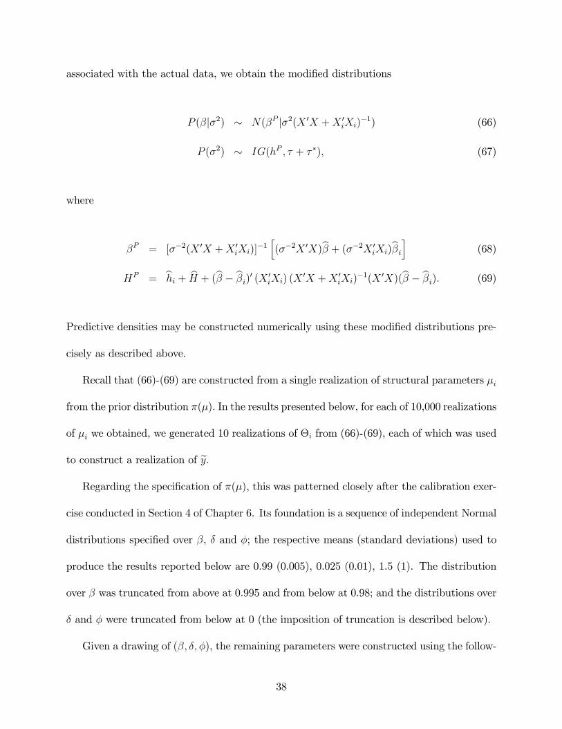
associated with the actual data, we obtain the modi�ed distributions

P (�j�2) � N(�P j�2(X 0X +X 0iXi)

�1) (66)

P (�2) � IG(hP ; � + � �); (67)

where

�P = [��2(X 0X +X 0iXi)]

�1h(��2X 0X)b� + (��2X 0

iXi)b�ii (68)

HP = bhi + bH + (b� � b�i)0 (X 0iXi) (X

0X +X 0iXi)

�1(X 0X)(b� � b�i): (69)

Predictive densities may be constructed numerically using these modi�ed distributions pre-

cisely as described above.

Recall that (66)-(69) are constructed from a single realization of structural parameters �i

from the prior distribution �(�): In the results presented below, for each of 10,000 realizations

of �i we obtained, we generated 10 realizations of �i from (66)-(69), each of which was used

to construct a realization of ey:Regarding the speci�cation of �(�), this was patterned closely after the calibration exer-

cise conducted in Section 4 of Chapter 6. Its foundation is a sequence of independent Normal

distributions speci�ed over �; � and �; the respective means (standard deviations) used to

produce the results reported below are 0.99 (0.005), 0.025 (0.01), 1.5 (1). The distribution

over � was truncated from above at 0.995 and from below at 0.98; and the distributions over

� and � were truncated from below at 0 (the imposition of truncation is described below).

Given a drawing of (�; �; �), the remaining parameters were constructed using the follow-

38

ing sequence of steps. Using � = 1=%� 1 and �; � was constructed as described in Chapter

6 as the value necessary for matching the steady state investment/output ratio with its

empirical counterpart:

� =

�� + %

�

�i

y(70)

=

�� + %

�

�0:175:

In addition, � was restricted to lie between 0.15 and 0.4. Likewise, ' was constructed as the

value necessary for matching the steady state consumption/output ratio with its empirical

counterpart:

' =1

1 + 2(1��)c=y

(71)

=1

1 + 2(1��)0:825

:

Next, � was used to construct a realization of the implied trajectory of the physical capital

stock fktgTt=1 using the perpetual inventory method. Along with the realization of �, this in

turn was used to generate a realization of the Solow residual flog ztgTt=1 : The growth rate

of log zt; the parameter g; was then calculated and used to construct the growth rate of the

arti�cial realization of output: gy = g=(1 � �): To maintain consistency with the unit-root

speci�cation for output, the AR parameter � was �xed at 1. Finally, � was constructed as

the standard deviation of � log zt:

To summarize, a drawing �i from �(�) was obtained by drawing (�; �; �) from their

respective Normal densities, and then constructing (�; '; gy; �) as described above. The

39

truncation restrictions noted above were imposed by discarding any �i that included an

element that fell outside of its restricted range. Approximately 15% of the 100,000 total

drawings of �i we obtained were discarded in this application.

Given a successful drawing of �i, fyitgT �

t=1 was simulated from (63) as described above.

Recall that this series is measured in terms of logged deviations of the level of output from

steady state. Thus a �nal adjustment is necessary to convert yit to a measure of the corre-

sponding level of output. The steady state trajectory of output is given by

yt = y0(1 + gy)t; (72)

where y0 represents an arbitrary initial steady state value (subsequent �rst-di¤erencing elim-

inates it from the analysis). Let the level of output corresponding with yit be given by Yit:

Then

yit = log

�Yit

y0(1 + gy)t

�; (73)

and thus the theoretical characterization of the level of output is given by

Yit = y0(1 + gy)teyit : (74)

It is the �rst di¤erence of the log of Yit that is used to estimate (52) in the numerical

integration algorithm described above.

The results of this exercise are presented in Table 9.1 and Figure 9.1. The table presents

posterior means and standard deviations of �; the �gure illustrates the actual data, point

forecasts and 95% coverage intervals. Five sets of estimates are presented: those obtained

40

in the absence of theoretical restrictions imposed by �(�); and four sets obtained using

alternative speci�cations of � �=� : 1, 2, 5, 10. (Point forecasts obtained given the restrictions

imposed by �(�) are virtually indistinguishable from those obtained in the absence of �(�);

thus only the latter are illustrated in the �gure.) Recall that � �=� measures the ratio of

arti�cial to actual degrees of freedom used in the construction of P (�j�2) and P (�2) in (66)

and (67). The greater is this ratio, the greater is the in�uence of �(�) in the analysis.19

Table 9.1. Posterior Estimates of the AR(2) Model� �=� �

0�1

�2

�

Means0 0.0030 0.384 0.041 0.00961 0.0036 0.242 0.073 0.00952 0.0038 0.191 0.076 0.00815 0.0042 0.139 0.073 0.007210 0.0043 0.113 0.071 0.0069Std. Devs.0 0.0008 0.072 0.071 0.00051 0.0007 0.063 0.061 0.00062 0.0006 0.050 0.049 0.00055 0.0004 0.037 0.037 0.000510 0.0003 0.030 0.030 0.0006

Three aspects of the changes in parameter estimates obtained in moving from � �=� = 0 to

� �=� = 10 are notable. First, posterior means of �1are reduced by a factor of 3, implying that

�uctuations in �yt become increasingly less persistent as the in�uence of the RBC model is

increased. Second, the posterior standard deviations associated with��0�0�2

�are reduced

by a factor of 2. Third, posterior means of � fall from 0.0096 to 0.0069, approaching the

standard deviation of log zt of 0.0067 obtained under the benchmark parameterization of the

model in the calibration exercise conducted in Chapter 6 (summarized in Table 6.4). All

19Results obtained using ��=� = 100 closely resemble those obtained using ��=� = 10; thus this caseappears to approximate a limiting scenario.

41

three factors help account for the increased precision of forecasts that results from increases

in � �=� , as illustrated in Figure 9.1.

Figure 9.1. Predictive Densities

To quantify this shrinkage, Table 9.2 reports the percentage di¤erence in the levels of

output that de�ne upper- and lower-95% coverage intervals at 1, 4, 8, and 12-quarter forecast

horizons for all �ve sets of forecasts. Shrinkage is noticeable even at the 1-quarter horizon,

falling from 4% to 3% in moving from � �=� = 0 to � �=� = 10. Respective shrinkages at the

4, 8, and 12-quarter horizons are from 9.75% to 6%, 13% to 8.3%, and 15.75% to 10%.

Table 9.2. Coverage-Interval Spreads (%)

42

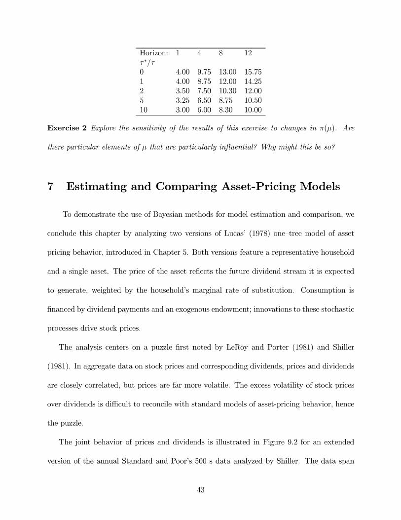
Horizon: 1 4 8 12� �=�0 4.00 9.75 13.00 15.751 4.00 8.75 12.00 14.252 3.50 7.50 10.30 12.005 3.25 6.50 8.75 10.5010 3.00 6.00 8.30 10.00

Exercise 2 Explore the sensitivity of the results of this exercise to changes in �(�). Are

there particular elements of � that are particularly in�uential? Why might this be so?

7 Estimating and Comparing Asset-Pricing Models

To demonstrate the use of Bayesian methods for model estimation and comparison, we

conclude this chapter by analyzing two versions of Lucas�(1978) one�tree model of asset

pricing behavior, introduced in Chapter 5. Both versions feature a representative household

and a single asset. The price of the asset re�ects the future dividend stream it is expected

to generate, weighted by the household�s marginal rate of substitution. Consumption is

�nanced by dividend payments and an exogenous endowment; innovations to these stochastic

processes drive stock prices.

The analysis centers on a puzzle �rst noted by LeRoy and Porter (1981) and Shiller

(1981). In aggregate data on stock prices and corresponding dividends, prices and dividends

are closely correlated, but prices are far more volatile. The excess volatility of stock prices

over dividends is di¢ cult to reconcile with standard models of asset-pricing behavior, hence

the puzzle.

The joint behavior of prices and dividends is illustrated in Figure 9.2 for an extended

version of the annual Standard and Poor�s 500 s data analyzed by Shiller. The data span

43

1871-2004, and are contained in the �le S&PData.txt, available at the textbook website.

Figure 9.2. Stock Prices and Dividends (Logged Deviations from Trend)

The data depicted in the �gure are measured as logged deviations from a common trend

(details regarding the trend are provided below). Prices are far more volatile than dividends:

respective standard deviations are 40.97% and 22.17%. The correlation between the series

is 0.409. As discussed below, absent this correlation virtually any preference speci�cation

can account for the observed pattern of volatility in Lucas�one-tree environment, if coupled

with a su¢ ciently volatile endowment process. The problem is that endowment innovations

weaken the link between price and dividend movements. Accounting for both the high

volatility and correlation patterns observed in the data represents the crux of the empirical

challenge facing the model.

44

The analysis presented here follows that of DeJong and Ripoll (2004), which is based on

the data measured through 1999. The �rst version of the model features CRRA preferences;

the second features preferences speci�ed following Gul and Pesendorfer (2004), under which

the household faces a temptation to deviate from its intertemporally optimal consumption

plan by selling its entire holding of shares and maximizing current-period consumption. This

temptation imposes a self-control cost that a¤ects the household�s demand for share holdings.

DeJong and Ripoll�s analysis centers on the relative ability of these models to account for

the joint behavior of prices and dividends.

Each version of the model reduces to a system of three equations: a pricing kernel

that dictates the behavior of pt, and laws of motion for dividends (dt) and the household�s

endowment (qt), which are taken as exogenous. Dropping time subscripts, so that pt and pt+1

are represented as p and p0; etc., and letting MRS denote the marginal rate of substitution

between periods t and t+ 1; the equations are given by

p = �Et [MRS � (d0 + p0)] ; (75)

log d0 = (1� �d) log(d) + �d log(d) + "dt (76)

log q0 = (1� �q) log(q) + �q log(q) + "qt; (77)

with j�ij < 1; i = d; q; and 2664 "dt"qt

3775 � IIDN(0;�): (78)

45

Under CRRA preferences, (75) is parameterized as

p = �Et(d0 + q0)�

(d+ q)� (d0 + p0); (79)

where > 0measures the degree of relative risk aversion. Regarding the stock-price volatility

puzzle, notice that a relatively large value of intensi�es the household�s desire for main-

taining a smooth consumption pro�le, leading to an increase in the predicted volatility of

price responses to exogenous shocks. Thus any amount of price volatility can be captured

through the speci�cation of a su¢ ciently large value of : However, increases in entail the

empirical cost of decreasing the predicted correlation between pt and dt; since increases in

heighten the role assigned to qt in driving price �uctuations. This is the puzzle in a nutshell.

Under self-control preferences, the momentary and temptation utility functions are pa-

rameterized as

u(c) =c1�

1� ; (80)

v(c) = �c�

�; (81)

with > 0; � > 0; and 1 > � > 0. These imply the following speci�cation for the pricing

kernel:

p = �E

24 (d0+q0)�

(d+q)� + �(d+ q) �(d0 + q0)��1 � (d0 + q0 + p0)��1

�1 + �(d+ q)��1+

35 [d0 + p0] : (82)

Notice that when � = 0, there is no temptation, and the pricing equation reduces to the

CRRA case.

46

To consider the potential for temptation in helping to resolve the stock-price volatility

puzzle, suppose � > 0: Then given a positive shock to either d or q, the term

�(d+ q) �(d0 + q0)��1 � (d0 + q0 + p0)��1

�;

which appears in the numerator of the pricing kernel, increases. However, if �� 1 + > 0,

i.e., if the risk-aversion parameter > 1, then the denominator of the kernel also increases. If

the increase in the numerator dominates that in the denominator, then higher price volatility

can be observed under temptation than in the CRRA case.

To understand this e¤ect, note that the derivative of the utility cost of self-control with

respect to wealth is positive given � < 1; so that v(:) is concave: v0(d0+e0)�v0(d0+e0+p0) > 0.

That is, as the household gets wealthier, self-control costs become lower. A reduction in self-

control costs serves to heighten the household�s incentive to save, and thus its demand for

asset holdings. Thus an exogenous shock to wealth increases share prices beyond any increase

resulting from the household�s incentives for maintaining a smooth consumption pro�le. This

explains why it might be possible to get higher price volatility in this case. Whether this

extension is capable of capturing the full extent of the volatility observed in stock prices,

while also accounting for the close correlation observed between prices and dividends, is the

empirical question to which we now turn.

The �rst empirical objective is to obtain parameter estimates for each model. This

is accomplished using as observables Xt = (pt dt)0; which as noted are measured as logged

deviations from a common trend. Regarding the trend, Shiller�s (1981) analysis was based on

the assumption that dividends and prices are trend stationary; DeJong (1992) and DeJong

47

and Whiteman (1991, 1994b) provided subsequent empirical support for this assumption.

Coupled with the restriction imposed by the asset-pricing kernel between the relative steady

state levels of dividends and prices, this assumption implies a restricted trend-stationarity

speci�cation for prices.

Regarding steady states, since fdtg and fqtg are exogenous, their steady states d and q

are simply parameters. Normalizing d to 1 and de�ning � = q

d, so that � = q; the steady

state value of prices implied by (79) for the CRRA speci�cation is given by

p =�

1� �d =�

1� � : (83)

Letting � = 1=(1+r), where r denotes the household�s discount rate, (83) implies p=d = 1=r.

Thus as the household�s discount rate increases, its asset demand decreases, driving down

the steady state price level. Empirically, the average price/dividend ratio observed in the

data serves to pin down � under this speci�cation of preferences.

Under the temptation speci�cation, the steady state speci�cation for prices implied by

(82) is given by

p = � (1 + p)

"(1 + �)� + � (1 + �)��1 � � (1 + � + p)��1

(1 + �)� + � (1 + �)��1

#: (84)

The left-hand-side of this expression is a 45-degree line. The right-hand side is strictly con-

cave in p, has a positive intercept, and a positive slope that is less than one at the intercept.

Thus (84) yields a unique positive solution for p for any admissible parameterization of the

model. An increase in � causes the function of p on the right-hand-side of (84) to shift down

48

and �atten, thus p is decreasing in �. The intuition for this is that an increase in � represents

an intensi�cation of the household�s temptation to liquidate its asset holdings. This drives

down its demand for asset shares, and thus p. Note the parallel between this e¤ect and that

generated by an increase in r, or a decrease in �, which operates analogously in both (83)

and (84).

Returning to the problem of detrending, given the value of p=d implied under either (83)

or (84), the assumption of trend-stationarity for dividends, coupled with this steady state

restriction yields:

ln(dt) = �0 + �1t (85)

ln(pt) =

��0 + ln

�p

d

��+ �1t:

Thus detrending is achieved by computing logged deviations of prices and dividends from the

restricted trajectories given in (85). Since the restrictions are a function of the collection of

deep parameters �, the raw data must be re-transformed for every re-parameterization of the

model. Speci�cally, given a particular speci�cation of �, which implies a particular value for

p=d, logged prices and dividends are regressed on a constant and linear time trend, given the

imposition of the parameter restrictions indicated in (85). Deviations of the logged variables

from their respective trend speci�cations constitute the values of Xt that correspond with

the speci�c parameterization of �.20

Under the CRRA speci�cation, the collection of parameters to be estimated are the

discount factor �; the risk-aversion parameter ; the AR parameters �d and �q; the standard

20The GAUSS procedure ct.prc is available for use in removing a common trend from a collection ofvariables.

49

deviations of innovations to d and q; denoted as �"d and �"q; the correlation between these

innovations corr("d; "q); and the steady state ratio � =q

d: Under the temptation speci�cation,

the curvature parameter � and the temptation parameter � are added to this list.

In specifying prior distributions, DeJong and Ripoll placed an emphasis on standard

ranges of parameter values, while assigning su¢ cient prior uncertainty to allow the data

to have a nontrivial in�uence on their estimates. The priors they used for this purpose

are summarized in Table 9.X. In all cases, prior correlations across parameters are zero;

and each of the informative priors we specify is normally distributed (but truncated when

appropriate).

Consider �rst the parameters common across both models. The prior mean (standard

deviation) of the discount factor � is 0.96 (0.02), implying an annual discount rate of 4%.

(This compares with an average dividend/price ratio of 4.6% in the data.) The prior for the

risk aversion parameter is centered at 2 with a standard deviation of 1. A non-informative

prior is speci�ed over the covariance matrix of the shocks �, proportional to det(�)�(m+1)=2

(where m is the dimension of �; or 2 in this case), and the priors over the persistence

parameters (�d; �e) are centered at 0.9, with standard deviations of 0.05. The prior over �

= q=d is more problematic, as neither the literature nor a priori guidance is available to

aid in its speci�cation. DeJong and Ripoll considered two alternative speci�cations of prior

means (standard deviations) for �: 5 (3); 10 (5). In so doing, they found that the data are

relatively uninformative regarding the location of �, so that the prior dominates the posterior

along this dimension. They also found that the prior over � turned out have little in�uence

both on the �t of the competing models and on estimates of the additional parameters. Here

we report results obtained using the (10, 5) speci�cation. Finally, the priors over (�; �d; �e)

50

are truncated from below at zero and from above at one, and the prior over � is truncated

from below at zero.

Priors for the self-control parameters � and � were speci�ed by focusing on the implica-

tions they carry for the steady state relationship between prices and dividends, as indicated

in (84). Note that along with � and �, the parameters �, and � also in�uence this rela-

tionship. When � = 0, the model reverts to the CRRA case, under which the prior over � is

centered on 0.96, implying an annual rate of return of 4%, or a steady state price/dividend

ratio of 24. As noted, the average rate of return in the data is 4.6%, implying an average

price/dividend ratio of approximately 22. Thus parameterizations of � and � were chosen

with this ratio as an approximate target. Fixing �, and � at their prior means, (�; �)

combinations in the respective ranges ([0, 0.001], [0, 0.75]) deliver this behavior. Increasing

� by one prior standard deviation, up to 0.98, moves these ranges to ([0, 0.006], [0, 0.8]);

re-centering � at 0.96 and decreasing by one standard deviation to 1 moves these ranges

to ([0, 0.014], [0, 0.8]); and re-centering and decreasing � by one standard deviation to 5

moves these ranges to ([0, 0.004], [0, 0.7]). Thus notice that small changes in � can have

large impacts on steady state price/dividend values, while changes in � have relatively small

impacts. Recall the intuition behind the impact of �: as the household�s temptation to

consume increases, its demand for asset holdings decreases, thus driving down p. In light

of these calculations, DeJong and Ripoll speci�ed a normal distribution for � centered and

truncated from below at 0, with a standard deviation of 0.01; and a normal distribution for

� centered at 0.4 with a standard deviation of 0.2, truncated from below at 0 and from above

at 1.

The models were estimated using the sequential importance sampling procedure described

51

in Section 4. A multivariate t distribution was speci�ed for I(�j�); centered initially on prior

means speci�ed for the individual elements of �: The initial covariance matrix speci�ed for

I(�j�) was diagonal, with standard deviations speci�ed as two times larger than the standard

deviations speci�ed under the prior. A second speci�cation of I(�j�) was then constructed

using the estimated posterior mean and covariance matrix obtained for � based on drawings

from the initial sampler. After several rounds moment calculations converged (subject to

numerical sampling error) to those reported below.

Due to the method used to detrend the data, the algorithm used to facilitate integration

works as follows. Obtain a drawing of � from I(�j�): Calculate p=d based on this drawing,

and detrend the raw data using (85). Solve the model, and evaluate the likelihood function

associated with the corresponding state-space representation. Calculate the weight w(�)

associated with the drawing, along with functions of interest g(�): Finally, compute weighted

averages gN as in (25) given N replications of this process.

7.1 Estimates

Posterior means and standard deviations obtained in this manner for both model spec-

i�cations are presented in Table 9.3. For the CRRA speci�cation, marginal posterior dis-

tributions of parameters are graphed in Figure 9.3; for the temptation speci�cation, these

distributions are graphed in Figure 9.4.

Table 9.3. Parameter Estimates

52

� � � �d �q �"d �"q �"d;"qq

d

Means:Prior 0.960 2.000 0.0000 0.4 0.900 0.900 UN UN UN 10.00CRRA 0.957 2.884 NA NA 0.876 0.913 0.114 0.097 0.313 10.68Self-Con. 0.966 1.973 0.00286 0.30 0.880 0.911 0.115 0.154 0.290 5.95Std. Dev.:Prior 0.020 1.000 0.01 0.2 0.050 0.050 UN UN UN 5.00CRRA 0.004 0.814 NA NA 0.033 0.026 0.007 0.035 0.124 4.39Self-Con. 0.007 0.422 0.00182 0.14 0.027 0.023 0.007 0.034 0.108 3.22

Posterior Correlations ; �"q ; �"d;"q �"q; �"d;"q �"d;"q ;

q

d

CRRA -0.836 -0.302 0.165 0.520Self-Con. -0.718 -0.343 0.047 0.553

Notes: UN denotes �uninformative prior�; NA denotes �not applicable�; and �x;y denotescorrelation between x and y.

For the CRRA speci�cation. the posterior distribution of � is centered very close to the

prior (with respective means of 0.957 and 0.96), but is much more tightly distributed (its

standard deviation of 0.004 is �ve times less than the prior�s). In contrast, the posterior and

prior dispersions of are similar (respective standard deviations are 0.814 and 1), while the

posterior distribution is moderately right-shifted relative to the prior (respective means are

2.884 and 2). Thus the data indicate a somewhat higher degree of risk aversion than was

embodied in the prior, but not by a dramatic amount: the means di¤er by less than one

prior standard deviation. Regarding the shocks, the persistence of the endowment shock is

greater than that of the dividend shock (posterior means of �d and �e are 0.876 and 0.913,

with standard deviations of 0.033 and 0.026), and the shocks are positively correlated (the

posterior mean of corr("d; "e) is 0.313, with posterior standard deviation of 0.124). Regarding

the size of the shocks, the posterior distributions of �"d and �"e have similar means (0.114 and

0.097, respectively); but the standard deviation of �"e is �ve times that of �"d, and is skewed

substantially to the right. Finally, as noted above, the prior and posterior distributions of

53

� = q=d are virtually indiscernible, indicating that the data are uninformative regarding the

location of this ratio.

Figure 9.3. Parameter Estimates, CRRA Preferences

To gain intuition for these results, it is important to keep in mind that the empirical

problem confronting the model is largely two-dimensional: simultaneously account for the

relatively high volatility of stock prices, and the close correlation observed between prices

and dividends. Four parameters play a critical role in confronting this problem. First,

large values of �"e and � are useful in helping the model along the former dimension: by

respectively increasing the volatility and importance of the household�s endowment in the

budget constraint, these parameters serve to increase the volatility of stock prices without

requiring an increase in the volatility of dividends. But these e¤ects are harmful along

54

the latter dimension: they serve to weaken the correlation between movements in prices and

dividends. However, this harm can be o¤set given a large corresponding value of corr("d; "e),

since this boosts the correlation between dividends and the endowment process, and thus

between dividends and prices. Finally, large values of provide help along the former

dimension by boosting the volatility of the household�s marginal rate of substitution for a

given volatility of consumption. But this again serves to weaken the correlation between

prices and dividends, because dividend �uctuations do not constitute the exclusive source of

�uctuations in consumption.

These considerations are helpful in understanding, for example, why the posterior distri-

bution of is only moderately right-shifted relative to the prior, and why the data clearly

favor a positive value for corr("d; "e). They are also helpful in interpreting the posterior

correlations estimated between the parameters of the model. Among the eight parameters

featured in this version of the model, there are four nontrivial posterior correlations (reported

in Table 9.3): between and �"e (-0.836); and corr("d; "e) (-0.302); �"e and corr("d; "e)

(0.165); and corr("d; "e) and � (0.520). So for example, given a relatively large value of

�"e, corr("d; "e) is also relatively large, and is relatively small: adjustments in these latter

parameters help combat the decreased dividend/price correlation associated with the large

value of �"e.

Turning to results obtained using the temptation speci�cation, the estimates obtained

for the parameters common to both the self-control and CRRA speci�cations are relatively

distinct. Most notably, the posterior mean of � increases by approximately one standard

deviation under the self-control speci�cation; the means of and � decrease by approximately

one standard deviation; and the mean of �"e increases by more than 1.5 standard deviations.

55

Anticipating the discussion of �t to follow, the decreases in and � will serve to increase

the correlation between prices and dividends in the model, while dampening the volatility of

prices; the increase in �"e will have the opposite e¤ect. This raises the question of why these

o¤setting factors arise. The key lies in reconsidering the relationship between steady state

prices and dividends given in (84). Movements away from zero by the self-control parameters

� and � cause sharp declines in the steady state price/dividend ratio; decreases in and

�, and increases in �, can serve to o¤set these e¤ects. Thus it appears that the altered

estimates of , � and � arise from an empirical preference for non-zero values of � and �;

the posterior estimates of these self-control parameters con�rm this observation.

Figure 9.4. Parameter Estimates, Self-Control Preferences

56

Figure 9.4, continued. Parameter Estimates, Self-Control Preferences

The posterior mean of � is 0.3, roughly one posterior standard deviation below its prior

mean, but still signi�cantly higher than zero. And the posterior mean of � is 0.00286, which

coincides closely with its mode, and lies approximately 1.5 posterior standard deviations

above the prior mode of zero. To appreciate the quantitative signi�cance of this estimate,

consider two alternative calculations. First, returning to (84), if , �, � and � are �xed

at their posterior means, an increase of � from zero to 0.00286 implies a decrease in the

steady state price/dividend ratio from approximately 28 to 20.46, implying an increase in

annual average returns from 3.57% to 4.89%. In other words, a household endowed with the

self-control preferences associated with these parameter estimates would demand an annual

�return premium�over a household endowed with CRRA preferences of 1.32%, representing

57

a 36% di¤erence. Second, consider the quantity of steady state consumption a household

endowed with the temptation speci�cation we estimate would be willing to sacri�ce in order

to be rid of this temptation. This is the value x such that

u(c� x) = u(c) + v(c)� v(ec);where here ec denotes the steady state value of temptation consumption. Using posteriormeans of parameter estimates, the implied value of x amounts to 5.25% of c. Thus these

results support for the presence of a quantitatively signi�cant temptation e¤ect in the data.

7.2 Model Comparison

To assess the relative ability of the competing models to account for the behavior of

dividends and prices, DeJong and Ripoll conducted a moment-based posterior-odds compar-

ison following Geweke (1999b), as described in Section 5. Four moments were chosen for

comparison: the standard deviations of prices and dividends �p and �d; the ratio of standard

deviations �d=�p; and the correlation between prices and dividends corr(p; d): In order to

characterize implications for these moments conveyed by the data, posterior distributions

were constructed using a six-lag VAR speci�ed for the data. Posterior means and standard

deviations obtained using the data and both versions of the model are reported in Table 9.4.

Corresponding posterior-odds calculations were obtained by approximating the integrals in

(50) using the kernel density approximation given by (51), with a density kernel provided by

the Normal distribution. These are also reported in Table 9.4. Finally, marginal posterior

distributions over these statistics obtained under the CRRA and self-control speci�cations

58

are depicted in Figures 9.5 and 9.6. For comparison, corresponding distributions obtained

using the VAR speci�cation are also depicted in both �gures.

Table 9.4. Summary Statistics

�p �d�d�p

�p;dMeans:VAR 0.620 0.268 0.448 0.672CRRA 0.434 0.244 0.571 0.536Self-Control 0.418 0.248 0.608 0.564Std. Dev.:VAR 0.183 0.065 0.095 0.178CRRA 0.067 0.041 0.101 0.079Self-Control 0.069 0.035 0.125 0.101

Notes: VAR statistics summarize �at-prior posterior distributions associated with a six-lag vector autoregression; �x denotes the standard deviation of the logged deviation of xfrom its steady state value; and �x;y denotes the correlation between logged deviations fromsteady state values of x and y.

59

Figure 9.5. Summary Statistics, CRRA Preferences

Regarding the distributions obtained using the VAR speci�cation, note that the distrib-

utions over �p and corr(p; d) exhibit considerable skewness. As a result, e.g., the posterior

mean of �p (0.62) lies considerably above its sample average of 0.406 (computed using the

data measured through 1999).

Figure 9.6. Summary Statistics, Self-Control Preferences

The relative performance of the competing models in matching the data along these

dimensions is very similar. Along the �p dimension, respective posterior means (standard

deviations) are 0.62 (0.183) in the data, 0.434 (0.067) under the CRRA speci�cation, and

0.418 (0.069) under the self-control speci�cation. Along the corr(p; d) dimension, respective

60

means (standard deviations) are 0.672 (0.178), 0.536 (0.079) and 0.564 (0.101). These dif-

ferences translate into a posterior-odds ratio of 2.4:1 in favor of the self-control speci�cation,

which constitutes �very slight evidence� in favor of the self-control speci�cation according

to Je¤reys�(1961) guidelines. Thus while the parameter estimates reported above are sup-

portive of the presence of a non-trivial self-control a¤ect, the a¤ect fails to translate into

a signi�cant improvement over the account of the stock-price volatility puzzle provided by

CRRA preferences.

61

References

[1] Bauwens, L. and Lubrano, M. 1998. �Bayesian Inference on GARCH Models using the

Gibbs Sampler.�The Econometrics Journal 1: C23-C46.

[2] Bauwens, L., Lubrano, M. and Richard, J. F. 1999. Bayesian Inference in Dynamic

Econometric Models. Oxford: Oxford University Press.

[3] Chib, S. and Greenberg, E. 1995. �Understanding the Metropolis-Hastings algorithm,"

The American Statistician 49:327-335.

[4] DeJong, D.N. 1992. �Co-Integration and Trend-Stationarity in Macroeconomic Time

Series,�Journal of Econometrics 52:347-370.

[5] DeJong, D. N., Ingram, B. F. 2001. �The Cyclical Behavior of Skill Acquisition,�Review

of Economic Dynamics 4:536-561.

[6] DeJong, D. N., Ingram, B. F. and Whiteman, C. H. 1993. �Evaluating VARs with

Monetary Business Cycle Priors�, Proceedings of the American Statistical Association,

Bayesian Statistical Science Section, 1993: 160-169.

[7] DeJong, D. N., Ingram, B. F. and Whiteman, C. H. 2000a. �Keynesian Impulses Ver-

sus Solow Residuals: Identifying Sources of Business Cycle Fluctuations,� Journal of

Applied Econometrics 15:311-329.

[8] DeJong, D. N., Ingram, B. F. and Whiteman, C. H. 2000b. �A Bayesian Approach to

Dynamic Macroeconomics,�Journal of Econometrics 98:203-223.

62

[9] DeJong, D.N., Liesenfeld, R. and Richard, J.-F. 2005. �A Non-Linear Forecasting Model

of GDP Growth,�Review of Economics and Statistics, forthcoming.

[10] DeJong, D. N. and Ripoll, M. 2004. �Self-Control Preferences and the Volatility of Stock

Prices,�University of Pittsburgh working paper.

[11] DeJong, D.N. and Whiteman, C.H. 1991. �The Temporal Stability of Dividends and

Stock Prices: Evidence from the Likelihood Function,� American Economic Review

81:600-617.

[12] DeJong, D.N. and Whiteman, C.H. 1994a. �The Forecasting Attributes of Trend- and

Di¤erence-Stationary Representations for Macroeconomic Time Series,�Journal of Fore-

casting 13:279-297.

[13] DeJong, D.N. and Whiteman, C.H. 1994b. �Modeling Stock Prices Without Pretending

to Know How to Induce Stationarity,�Econometric Theory 10:701-719.

[14] Del Negro, M. and Schorfheide, F. 2004. �Priors from General Equilibrium Models for

VARs,�International Economic Review 45:643-673.

[15] Doan, T., Litterman, R. and Sims, C. 1984. �Forecasting and Conditional Projection

Using Realistic Prior Distributions,�Econometric Reviews 3:1-100.

[16] Fernandez-Villaverde, J. and Rubio-Ramirez, J.F. 2004. �Comparing Dynamic Equilib-

rium Models to Data: A Bayesian Approach." Journal of Econometrics 123:153-187.

[17] Geweke, J. 1988. �Antithetic Acceleration of Monte Carlo Integration in Bayesian In-

ference,�Journal of Econometrics 38:73-89.

63

[18] Geweke, J. 1989. �Bayesian Inference in Econometric Models using Monte Carlo Inte-

gration,�Econometrica 57:1317-1339.

[19] Geweke, J. 1992. �Evaluating the Accuracy of Sampling-Based Approaches to the Cal-

culation of Posterior Moments," in Bernardo, et al., Eds., Bayesian Statistics 4 Oxford:

Clarendon Press.

[20] Geweke, J. 1999a. �Using Simulation Methods for Bayesian Econometric Models: Infer-

ence, Development, and Communication,�Econometric Reviews 18:1-126.

[21] Geweke, J. 1999b. �Computational Experiments and Reality,�University of Iowa work-

ing paper.

[22] Gul, F. and Pesendorfer, W. 2004. �Self-Control, Revealed Preference and Consumption

Choice,�Review of Economic Dynamics 7:243-264.

[23] Hamilton, J.D. 1994. Time Series Analysis. Princeton: Princeton University Press.

[24] Heyde, C. C. and Johnstone, I. M. 1979. �On Asymptotic Posterior Normality for

Stochastic Processes,�Journal of the Royal Statistical Society Series B 41:184-189.

[25] Ingram, B. F. and Whiteman, C. H. 1994. �Supplanting the �Minnesota�Prior: Fore-

casting Macroeconomic Time Series Using Real Business Cycle Model Priors,�Journal

of Monetary Economics 34:497-510.

[26] Je¤reys, H. 1961. Theory of Probability, 3rd Ed. Oxford: Clarendon Press.

[27] Kloek, T. and van Dijk, H. K. 1978. �Bayesian Estimates of Equation System Parame-

ters: An Application of Integration by Monte Carlo,�Econometrica 46:1-19.

64

[28] Koop, G. 2003. Bayesian Econometrics. New York: Wiley.

[29] Leamer, E. E. 1978. Speci�cation Searches. New York: Wiley.

[30] LeRoy, S.F. and Porter, R.D. 1981. �Stock Price Volatility: Tests Based on Implied

Variance Bounds,�Econometrica 49:97-113.

[31] Ljungqvist, L. and T. Sargent. 2004. Recursive Macroeconomic Theory. Cambridge:

MIT Press.

[32] Nelson, C. and Plosser, C.H. �Trends and Random Walks in Macroeconomic Time

Series: Some Evidence and Implications,�Journal of Monetary Economics 10:139-162.

[33] Otrok, C. 2001. �On Measuring the Welfare Costs of Business Cycles,�Journal of Mon-

etary Economics 47:61-92.

[34] Pesaran, M.H. and Potter, S.M. 1997. �A Floor and Ceiling Model of US Output,�

Journal of Economic Dynamics and Control 21:661-695.

[35] Richard, J. F. and Zhang, W. 1997. �Accelerated Monte Carlo Integration: An Applica-

tion to Dynamic Latent Variable Models�In Mariano, R. Weeks, M. and Schuermann,

T., Eds., Simulation Based Inference in Econometrics: Methods and Applications. Cam-

bridge: Cambridge University Press.

[36] Richard, J. F. and Zhang, W. 2004. �E¢ cient High-Dimensional Monte Carlo Impor-

tance Sampling�University of Pittsburgh working paper.

[37] Robert, C. P. and Casella, G. 1999. Monte Carlo Statistical Methods. New York:

Springer-Verlag.

65

[38] Rubinstein, R. Y. 1981. Simulation and the Monte Carlo Method. New York: Wiley.

[39] Schorfheide, F. 2000. �Loss Function-Based Evaluation of DSGE Models." Journal of

Applied Econometrics 15:645-670.

[40] Schotman, P.C. and van Dijk, H.K. �On Bayesian Routes to Unit Roots,�Journal of

Applied Econometrics 6:387-401.

[41] Shiller, R.J. 1981. �Do Stock Prices Move too Much to be Justi�ed by Subsequent

Changes in Dividends?�American Economic Review 71:421-436.

[42] Shiryaev, A. N. 1995. Probability. Berlin: Springer Graduate Texts in Mathematics.

[43] Silverman, B.W. 1986. Density Estimation. London: Chapman and Hall.

[44] Sims, C. A. and Zha, T. 1998. �Bayesian Methods for Dynamic Multivariate Models,�

International Economic Review 39:949-968.

[45] Theil, H. and Goldberger, A. S. 1961. �On Pure and Mixed Statistical Estimation in

Economics,�International Economic Review 2:65-78.

[46] Yu, B. and P. Mykland. 1994. �Looking at Markov Samplers through CUSUM Path

Plots: A Simple Diagnostic Idea.� Technical Report 413. Department of Statistics,

University of California at Berkeley.

[47] Zellner, A. 1971. An Introduction to Bayesian Inference in Econometrics. New York:

Wiley.

66