Embed Size (px)
Citation preview

_________________________________________________________
Structural Motion Control
in MSC.NASTRAN _________________________________________________________
JULY 2011
MAVERICK UNITED CONSULTING ENGINEERS

Structural Motion Control in MSC.NASTRAN
2
TABLE OF CONTENTS
ACKNOWLEDGEMENTS ....................................................................................................................................... 3
LIST OF SYMBOLS AND NOTATIONS ............................................................................................................... 4
1.1 GL, ML PASSIVE STRUCTURAL MOTION CONTROL ....................................................................................... 7 1.1.1 Optimum Stiffness and Mass Distribution ...................................................................................................................................... 7 1.1.1.1 Concepts of Forced Frequency Response of Deterministic Periodic Harmonic Load Excitations ............................................................................. 7 1.1.1.2 Concepts of Forced Transient Response of Deterministic Load Excitations............................................................................................................ 10 1.1.1.3 Concepts of Forced Frequency Response of Deterministic Periodic Harmonic Base Excitations ........................................................................... 14 1.1.1.4 Concepts of Forced Transient Response of Deterministic Base Excitations ............................................................................................................ 15 1.1.1.5 Concepts of Forced Transient Response (Response Spectrum Analysis) of Random Non-Stationary Base Excitations .......................................... 16 1.1.2 Optimum Damping Distribution .................................................................................................................................................... 17 1.1.2.1 Elemental Damping Mathematical Models.............................................................................................................................................................. 17 1.1.2.2 Modal Damping Mathematical Models ................................................................................................................................................................... 26 1.1.2.3 Global Damping Mathematical Models ................................................................................................................................................................... 29 1.1.2.4 Damping Formulation Conclusions ......................................................................................................................................................................... 31 1.1.3 GL, ML Base Isolation Systems ..................................................................................................................................................... 32 1.1.3.1 Controlling Displacement Response From Harmonic Load Excitations .................................................................................................................. 32 1.1.3.2 Controlling Acceleration Response From Harmonic Load Excitations ................................................................................................................... 32 1.1.3.3 Base Isolation - Controlling Displacement Response From Harmonic Base Enforced Motion ............................................................................... 33 1.1.3.4 Base Isolation - Controlling Acceleration Response From Harmonic Base Enforced Motion ................................................................................. 34 1.1.3.5 Base Isolation – Controlling Force Transmitted Into Foundation From Harmonic Load Excitations ...................................................................... 36 1.1.4 GL, ML Tuned Mass Damper (TMD) Systems ............................................................................................................................ 37 1.1.4.1 Damped SDOF System Subject to Harmonic Force and Support Motion Excitations ............................................................................................. 40 1.1.4.2 Undamped Structure, Undamped TMD System Subject to Harmonic Force Excitation .......................................................................................... 41 1.1.4.3 Undamped Structure, Damped TMD System Subject to Harmonic Force Excitation .............................................................................................. 43 1.1.4.4 Undamped Structure, Damped TMD System Subject to Harmonic Support Motion ............................................................................................... 49 1.1.4.5 Damped Structure, Damped TMD System Subject to Harmonic Force and Support Motion .................................................................................. 51 1.1.4.6 TMD Analysis Summary (Warburton, 1982) .......................................................................................................................................................... 53 1.1.5 GL, ML Tuned Slosh Damper (TSD) Systems ............................................................................................................................. 55 1.1.5.1 When To Employ TSDs .......................................................................................................................................................................................... 55 1.1.5.2 Operations of TSDs ................................................................................................................................................................................................. 55 1.1.5.3 Deep or Shallow Tank? ........................................................................................................................................................................................... 63 1.1.5.4 Testing..................................................................................................................................................................................................................... 64 1.1.5.5 Miscellaneous Design Information .......................................................................................................................................................................... 65 1.1.5.6 Design Procedure for Deep Tank TSDs................................................................................................................................................................... 66
1.2 GL, ML ACTIVE STRUCTURAL MOTION CONTROL – CONTROL SYSTEM ANALYSIS ................................. 67
BIBLIOGRAPHY ..................................................................................................................................................... 68

Structural Motion Control in MSC.NASTRAN
3
ACKNOWLEDGEMENTS
My humble gratitude to the Almighty, to Whom this and all work is dedicated.
A special thank you also to my teachers at Imperial College of Science, Technology and Medicine, London and my
fellow engineering colleagues at Ove Arup and Partners London and Ramboll Whitbybird London.
Maverick United Consulting Engineers

Structural Motion Control in MSC.NASTRAN
4
LIST OF SYMBOLS AND NOTATIONS
Elemental Notations
{y} = displacement function
[N] = shape functions matrix
{f} = element forces in element axes including fixed end forces
{d} = element deformation in element axes
{b} = element body forces
[k] = element constitutive matrix
[m] = element mass matrix
[c] = element viscous damping matrix
{p} = element nodal loading vector
[T] = transformation matrix
W = work done by external loads
SDOF, MDOF and Modal Dynamic Equation of Motion Notations
m = SDOF mass
[M] = Global MDOF mass matrix
c = SDOF viscous damping constant
[C] = Global MDOF viscous damping matrix
k = SDOF stiffness
[K] = Global MDOF stiffness matrix
u = SDOF displacement
{u},{U}= Global MDOF displacement matrix
{P} = Global nodal loading vector
Mi, [M] = Modal (generalized) mass and modal (generalized) mass matrix
Ci, [C] = Modal (generalized) damping and modal (generalized) damping matrix
Ki, [K] = Modal (generalized) stiffness and modal (generalized) stiffness matrix
i, {i} = Modal displacement response and modal displacement response vector
SDOF Dynamic Notations
n = Natural circular frequency, (k/m)1/2
d = Damped natural circular frequency, n(1)1/2
= Frequency of forcing function
c = Viscous damping constant
ccr = Critical viscous damping constant, 2(km)1/2 = 2mn
= Damping ratio (fraction of critical), c/ccr
= Logarithmic decrement
SDOF Free Vibrational Notations
G = Complex starting transient response function, G = GR + iGI
SDOF Time Domain Loading and Transient and Steady-State Response Notations
P(t) = Loading function
p0 = Force excitation amplitude
p0/k = Static displacement
D(t) = Dynamic amplification factor

Structural Motion Control in MSC.NASTRAN
5
Dmax = Maximum dynamic amplification factor
u(t) = Displacement response, D(t)(p0/k)
umax = Maximum displacement response, Dmax(p0/k)
Modal Time Domain Loading and Transient and Steady-State Notations
{P(t)} = Loading function vector
Pi(t) = Modal loading function, Pi(t) = {i}T {P(t)}
p0i = Modal force excitation amplitude
p0i/Ki = Modal static displacement
Di (t) = Modal dynamic amplification factor
Di max = Modal maximum dynamic amplification factor
i(t) = Modal displacement response, i(t) = Di(t)p0i/Ki
i max = Modal maximum displacement response, i max = Di max p0i/Ki
{u(t)} = Displacement response vector, {u(t)} = []{(t)}
SDOF Frequency Domain Loading and Steady-State Response Notations
P(t) = SDOF Time domain harmonic loading function, P(t) = Real [ P()eit ]
P() = SDOF frequency domain complex harmonic loading function
p0 = SDOF harmonic loading amplitude
p0/k = SDOF static displacement
D() = SDOF (magnitude of the) dynamic amplification factor
Dresonant = SDOF (magnitude of the) dynamic amplification factor at resonance when n
Dmax = SDOF maximum (magnitude of the) dynamic amplification factor when = n(1-22)1/2
F() = SDOF complex displacement response function (FRF), F() = D()(p0/k)ei
H() = SDOF transfer function, H() = D()(1/k)ei
Fresonant = SDOF complex displacement response function at resonance, Fresonant = Dresonant(p0/k)ei
Fmax = SDOF complex maximum displacement response function, Fmax = Dmax(p0/k)ei
u(t) = SDOF time domain displacement response, u(t) = Real [ F()eit ]
uresonant = SDOF time domain displacement response at resonance, u(t) = Real [ Fresonant eit]
umax = SDOF time domain maximum displacement response, u(t) = Real [ Fmax eit]
Tr = SDOF transmissibility of displacement, acceleration or force
Modal Frequency Domain Loading and Steady-State Response Notations
{P(t)} = Time domain harmonic loading function vector, {P(t)} = Real [ {P()} eit ]
{P()} = Frequency domain complex harmonic loading function vector
Pi() = Modal frequency domain complex harmonic loading function vector, Pi() = {i}T {P()}
p0i = Modal harmonic loading amplitude
p0i/Ki = Modal static displacement
Di() = Modal (magnitude of the) dynamic amplification factor
Di resonant = Modal (magnitude of the) dynamic amplification factor at resonance when ni
Di max = Modal maximum (magnitude of the) dynamic amplification factor when = ni(1-2i2)1/2
i() = Modal complex displacement response function (FRF), i() = Di()p0i/Ki eii
i resonant = Modal complex displacement response function at resonance, i resonant = Di resonant p0i/Ki eii
i max = Modal complex maximum displacement response function, i max = Di max p0i/Ki eii
{u(t)} = Time domain displacement response vector, {u(t)} = Real [ []{()}eit ]
Additional Abbreviations

Structural Motion Control in MSC.NASTRAN
6
ML: Materially Linear
MNL: Materially Nonlinear
GL: Geometrically Linear
GNL: Geometrically Nonlinear
[] = matrix
{} = column vector
<> = row vector

Structural Motion Control in MSC.NASTRAN
7
1.1 GL, ML Passive Structural Motion Control
Methods of passive structural motion control are: -
i. Optimum stiffness and mass distribution
ii. Isolation systems
iii. Optimum damping distribution
iv. Tuned mass damper systems
1.1.1 Optimum Stiffness and Mass Distribution
1.1.1.1 Concepts of Forced Frequency Response of Deterministic Periodic Harmonic Load Excitations
In a modal forced frequency response analysis, the modal response in modal coordinates i and the modal response
in physical coordinates ui(t) are
The relative importance of each mode is encapsulated in the values of the modal responses i. However, the
physical response effects can be more critical from less significant modes (i.e. with lower modal responses)
due to the inherent shape of the eigenvector even if the scaling factor (i.e. the modal response) is smaller. The
following parameters are of particular interest in controlling the modal response: -
I. The modal mass and (the amplitude of the) modal force must be considered together as their
magnitudes are related to the arbitrary normalization of i. MAX normalization scales the
eigenvectors such that their maximum component is unity and all other components less than unity.
The relative magnitude of the modal mass between different modes scaled by MAX is not in itself an
indication of the relative importance of the particular mode as that also depends on the magnitude
and location of the applied load excitation, given by the amplitude of the modal force. To reduce the
modal response i, the modal mass should be maximized AND the amplitude of the modal force
should be minimized. The modal mass will be maximized if there is more structural mass in the
mode, hence the heavier the structure, the greater shall be the modal mass of most modes, and the
lower the modal response. The amplitude of the modal force will be minimized if the amplitude of
the applied force is minimized and if the location of the applied force corresponds to the DOF
with smaller components of the eigenvector. This is obvious from a physical viewpoint, as clearly
the modal response should be greater if the excitation is applied at the maximum locations of the
eigenvector. With MAX normalization, the value of the modal mass is still of significance. A graph
of (MAX normalized) modal mass versus modal frequency is most illustrative of the global and local
modes. The greater the modal mass, the lower will be the response assuming constant amplitude of
modal force. A very small modal mass (several orders of magnitude smaller than that of other
modes) obtained from MAX normalization indicates a local mode or an isolated mechanism. If the
applied force were to be located at the mechanism, the amplitude of the modal force may be
significant, and hence so may the modal response. If the distribution of mass is uniform, then
higher modes of the same type (for instance higher bending modes relative to the fundamental
bending mode) MAY have the same MAX normalized modal masses (simply supported beam
modal masses 0.5mL and cantilever beam modal masses 0.25mL). However other types of global
modes of higher frequency than the fundamental frequency may have lower modal masses. For
instance, the first torsional mode of a tower, which may be of a higher natural frequency than the first
bending mode, may have a lower modal mass. This means that higher frequency global modes can
also be significantly excited if the applied force was such that it corresponded to the greater values of
their eigenvector.
ti
iii
2
ni2
nii1i
i
2ni
0ii
i0iii
e)( alRe)t(u
/1
/2tan,e)(De)(D)( ii
ii M
p
K
p

Structural Motion Control in MSC.NASTRAN
8
Hence, the modal masses of each and every mode are values that can be compared if all the modes
had the same amplitude of modal force. The amplitude of the modal force for each and every mode
can be made to be the same if there is only one concentrated applied force at one DOF and if the
POINT normalization corresponding to that DOF is used for all modes. POINT normalization allows
the user to choose a specific DOF at which the modal displacements are set to 1 or –1. Hence, the
amplitude of the modal force for all modes will be the same and only the modal mass need to be
compared. In this case, there will be significant difference in the order of magnitude of different
global modes. The higher the modal mass with this method, the lower shall be the modal response.
However, this normalization is not recommended because for complex structures, the chosen
component may have very small values of displacement for higher modes causing larger numbers to
be normalized by a small number, resulting in possible numerical roundoff errors and ridiculously
higher modal masses. For instance, if the POINT normalization points to a DOF component which
does not really exist in a particular mode, than all the other eigenvector terms will be normalized by a
very small number, which will certainly result in numerical errors.
II. For ANY natural mode, the (magnitude of the) dynamic amplification factor, Di() becomes infinite
or is limited only by the modal damping of the particular mode when the excitation frequency
approaches the natural frequency of the mode. The higher the modal damping, the lower the
(magnitude of the) modal dynamic amplification factor, Di(). Hence, the modal amplification can
be reduced by either mistuning the frequencies of excitation and the modal natural frequencies
or by increasing the modal damping. Dimax occurs when /n = (1-22)1/2.
T5 VCR REAL MODAL ANALYSIS - MODAL MASS
0.000
25.000
50.000
75.000
100.000
125.000
150.000
175.000
200.000
225.000
250.000
0 5 10 15 20 25 30 35 40 45 50
Mode Number
Mo
da
l M
ass
(T
on
nes
)
Primary Tower
Bending Modes
Secondary Tower
Bending Modes
Cable Modes Cable Modes Cable ModesCable Modes
Primary Tower
Torsion Mode
0
1
2
3
4
5
6
0 1 2
Dy
na
mic
Am
pli
fica
tio
n F
acto
r, D
Frequency Ratio /n
Variation of D with Frequency Ratio For Different
Damping
zhi=0
zhi=0.1
zhi=0.2
zhi=1
zhi=2
2maxi
2
nii
22
ni2
i
12
1D
;
/2/1
1)(D

Structural Motion Control in MSC.NASTRAN
9
III. Higher modes are less significant then lower modes because of the higher natural frequency ni2 in
the expression for the modal response i.
Hence, in order to reduce the total steady-state response (by controlling the distribution of mass, stiffness and
damping) to a fixed frequency and amplitude of excitation, the following may be undertaken.
I. The structural mass distribution, stiffness distribution and boundary conditions are modified so
that there are no natural frequencies close to the frequency of excitation (and causing resonance) in
order to minimize the (magnitude of the) dynamic amplification factor, Di(). If the lowest natural
frequency can be made significantly greater than the excitation frequency, then all the natural modes
respond in a quasi-static manner to the excitation, and thus the response will only be dependent upon
the amplitude of excitation as the frequency is low enough to be considered static. If this cannot be
done, the natural modes should be tuned such that the excitation frequency is much greater than the
lower natural frequencies. The response of the lower modes will be governed by inertial forces (the
response of which is even lower than the quasi-static response) and the (magnitude of the) dynamic
amplification factor, Di() will be minimized. However, Di() of higher modes will be more
significant. But since ni2 features in the denominator of the modal response expression i, the higher
modes will produce a lower modal response (although the modal physical response could be
significant) when resonated.
II. The mass distribution of the structure is increased in order to increase the modal masses
(specifically of the modes with significant modal response i, but generally all), which in turn
reduces the modal response i. This however will lower the natural frequencies and will affect the
(magnitude of the) dynamic amplification factor, Di() of I.
III. The stiffness distribution of the structure is increased in order to increase the natural frequencies
ni2 (specifically of the modes with significant modal response i, but generally all), which feature in
the denominator of the modal response i expression. This will however affect the (magnitude of the)
dynamic amplification factor, Di() of I.
IV. The boundary conditions of the structure are altered in order to increase the natural frequencies ni2
(specifically of the modes with significant modal response i, but generally all), which feature in the
denominator of the modal response i expression. This will however affect the (magnitude of the)
dynamic amplification factor, Di() of I.
V. The location and direction of the applied load excitation is modified to not correspond to the large
locations of the modes with significant modal response i in order to reduce the amplitude of the
modal force, which in turn will reduce the modal response i.
VI. The damping distribution is modified such as to maximize the modal damping of the modes with
significant modal response i. This is done in order to minimize the (magnitude of the) dynamic
amplification factor, Di() and hence minimizing the modal response i. If resonance is unavoidable,
damping should be incorporated, as it is most efficient at resonance. For the design of explicit
dampers, it is necessary to find the location and range of the damping parameter for optimum
damping of a particular mode. The optimum location will clearly be at the position of the maximum
components of the eigenvector. Optimum values of the viscous damping coefficient c (Ns/m) depend
on the optimum modal damping obtained for a particular range of damping constant. There is always
a plateau where the values of the damping constant c will give the optimum (highest) modal
damping. This plateau range is obtained computationally by running repetitive complex modal
analysis (MSC.NASTRAN SOL 107) with varying damping constants, and observing the range
which gives the optimum damping for the structural mode that is to be damped.

Structural Motion Control in MSC.NASTRAN
10
1.1.1.2 Concepts of Forced Transient Response of Deterministic Load Excitations
In a modal forced transient response analysis, the modal response in modal coordinates i and the modal response
in physical coordinates ui(t) are
The relative importance of each mode is encapsulated in the values of the modal responses i. However, the
physical response effects can be more critical from less significant modes (i.e. with lower modal responses)
due to the inherent shape of the eigenvector even if the scaling factor (i.e. the modal response) is smaller. The
following parameters are of particular interest in controlling the modal response: -
I. The modal mass and (the amplitude of the) modal force must be considered together as their
magnitudes are related to the arbitrary normalization of i. MAX normalization scales the
eigenvectors such that their maximum component is unity and all other components less than unity.
The relative magnitude of the modal mass between different modes scaled by MAX is not in itself
an indication of the relative importance of the particular mode as that also depends on the
magnitude and location of the applied load excitation, given by the amplitude of the modal force.
To reduce the modal response i, the modal mass should be maximized AND the amplitude of the
modal force should be minimized. The modal mass will be maximized if there is more structural
mass in the mode, hence the heavier the structure, the greater shall be the modal mass of most
modes, and the lower the modal response. The amplitude of the modal force will be minimized if
the amplitude of the applied force is minimized and if the location of the applied force
corresponds to the DOF with smaller components of the eigenvector. This is obvious from a
physical viewpoint, as clearly the modal response should be greater if the excitation is applied at
the maximum locations of the eigenvector. With MAX normalization, the value of the modal mass
is still of significance. A graph of (MAX normalized) modal mass versus modal frequency is most
illustrative of the global and local modes. The greater the modal mass, the lower will be the
response assuming constant amplitude of the modal force. A very small modal mass (several orders
of magnitude smaller than that of other modes) obtained from MAX normalization indicates a local
mode or an isolated mechanism. If the applied force were to be located at the mechanism, the
amplitude of the modal force may be significant, and hence so may the modal response. If the
distribution of mass is uniform, then higher modes of the same type (for instance higher
bending modes relative to the fundamental bending mode) MAY have the same MAX
normalized modal masses (simply supported beam modal masses 0.5mL and cantilever beam
modal masses 0.25mL). However other types of global modes of higher frequency than the
fundamental frequency may have lower modal masses. For instance, the first torsional mode of a
tower, which may be of a higher natural frequency than the first bending mode, may have a lower
modal mass. This means that higher frequency global modes can also be significantly excited if the
applied force was such that it corresponded to the greater values of their eigenvector.
)t( )t(u
)t(D)t(D)t(
iii
2ni
0ii
0iii
ii M
p
K
p

Structural Motion Control in MSC.NASTRAN
11
Hence, the modal masses of each and every mode are values that can be compared if all the modes
had the same amplitude of modal force. The amplitude of the modal force for each and every mode
can be made to be the same if there is only one concentrated applied force at one DOF and if the
POINT normalization corresponding to that DOF is used for all modes. POINT normalization allows
the user to choose a specific DOF at which the modal displacements are set to 1 or –1. Hence, the
amplitude of the modal force for all modes will be the same and only the modal mass need to be
compared. In this case, there will be significant difference in the order of magnitude of different
global modes. The higher the modal mass with this method, the lower shall be the modal response.
However, this normalization is not recommended because for complex structures, the chosen
component may have very small values of displacement for higher modes causing larger numbers to
be normalized by a small number, resulting in possible numerical roundoff errors and ridiculously
higher modal masses. For instance, if the POINT normalization points to a DOF component which
does not really exist in a particular mode, than all the other eigenvector terms will be normalized by a
very small number, which will certainly result in numerical errors.
II. In general, Di(t) is a function of the natural circular frequency ni2 = Ki/Mi or the damped natural
circular frequency d, the time duration of loading td and the general time t. For a SDOF system,
Dimax can be found by differentiation and is a function of the natural circular frequency ni2 = Ki/Mi
or the damped natural circular frequency d and the time duration of loading td. A graph of Dimax
versus td / Ti is extremely illustrative of the maximum amplification that can be achieved for a
particular type of impulsive loading.
T5 VCR REAL MODAL ANALYSIS - MODAL MASS
0.000
25.000
50.000
75.000
100.000
125.000
150.000
175.000
200.000
225.000
250.000
0 5 10 15 20 25 30 35 40 45 50
Mode Number
Mo
da
l M
ass
(T
on
nes
)Primary Tower
Bending Modes
Secondary Tower
Bending Modes
Cable Modes Cable Modes Cable ModesCable Modes
Primary Tower
Torsion Mode
Response Spectrum
0
0.5
1
1.5
2
2.5
0 0.5 1 1.5 2 2.5 3 3.5 4 4.5
td/T i
Dim
ax

Structural Motion Control in MSC.NASTRAN
12
The above shows that the maximum dynamic amplification that can be produced from short duration
impulse loadings is two! Maximum amplifications of higher modes are represented by points to the
right of that for the fundamental mode.
On inspection of the red curve representing the ramp up load in duration td, it is apparent that when
the ramp is of a shorter duration td than the fundamental period T1 (i.e. td/T1 < 1.0), the amplification
is large decreasing from 2.0 to 1.0 (no dynamic amplification) when the duration equals the period.
Higher modes are less amplified as td/Ti becomes larger. If the duration is larger than the
fundamental period (i.e. td/T1 > 1.0), the amplification will be small. The yellow curve with a large
duration is simply a special case of the red curve with an instantaneous ramp (i.e. td/T1 = 0.0), hence
causing a dynamic amplification of 2.0. In conclusion, if the ramp is such that it is gradual
enough to be at least equal to the period of the fundamental mode (i.e. td/T1 > 1.0), the
amplification can be minimized.
On inspection of the green curve representing the impulsive loads, if the duration of the impulse td is
close to the period of the fundamental mode T1, the amplification is large (~1.5). Higher modes are
less amplified as td/Ti becomes larger. If the duration is much smaller than the fundamental period
(td/T1 < ~0.4), the amplification is less than unity, and hence not even the static response is observed
as the impulse to too fast for the structure to react. If the duration is much larger than the
fundamental period (td/T1 > 2.0), the amplification is small. The yellow curve with a small duration is
simply a special case of the green curve with an instantaneous impulse (i.e. td/T1 < ~0.2), hence
causing a dynamic amplification of less than 1.0 (i.e. less than static response). In conclusion, if the
impulsive load is much smaller in duration (td/T1 < ~0.4) or much larger in duration (td/T1 >
2.0) compared to the fundamental mode T1, the amplification can be minimized.
The fact that impulsive loads cause little amplification can also be quantified more directly than
employing the dynamic amplification. The response from a true impulse (t1/T < ~0.2) is readily
obtained as the unit impulse function can be brought outside the Duhamel’s or Convolution Integral.
The maximum modal response (not the dynamic amplification Di(t)) from an impulsive load (t1/T <
0.2), can be obtained simply as follows.
The above expression may seem to differ from the dynamic amplification approach where the
denominator contains the modal stiffness, i.e. modal mass times the square of the natural circular
frequency. This is because the above expression requires the explicit integration of the forcing
function. The dynamic amplification approach differs in the sense that the integral (i.e. Duhamel’s
Integral) is already classically integrated to obtain the expression D(t). Another equivalent
interpretation of the above relationship is from the basic consideration of the conservation of
momentum. The impacting particle (of small relative mass compared to mass of structure) imposes
an impulse I onto the structure. The magnitude of I can be calculated as mv where m is the small
mass and v the change of velocity at impact. If there is no rebound v is the approach velocity.
Conservation of momentum at impact requires the initial velocity of the structural mass to be I/M. A
lightly damped system then displays damped free vibration with an initial displacement of
point excitationat component almod where
damped)dp(1
undamped)dp(1
)dp()-h(t)t(
i
t
0i
dimaxi
t
0i
nimaxi
t
0i
i
i
M
M

Structural Motion Control in MSC.NASTRAN
13
approximately I/(dM), or an initial velocity of approximately I/M or an initial acceleration of
approximately Id/M.
The general derivation of the impulse force is a science in itself. Simple considerations can however
result in good approximations. As mentioned, an impacting particle (of small relative mass compared
to mass of structure) imposes an impulse I = Ft = mv onto the structure, where m and v are
known. Knowing that Ft is the area under the impulse curve, making an estimate of the shape of the
impulse curve and the duration t, we can thus estimate the peak amplitude. Hence, the impulse
curve is defined.
Hence, if the structure is tuned such that the period of the fundamental mode is much less than
the duration of the impulse (t1/T < 0.2), the amplification will be very low and can readily be
ascertained using the above relationship. Of course, higher modes may be amplified more than
the fundamental mode but would respond less because of the larger natural frequency ni2.
III. Higher modes are less significant then lower modes because of the higher natural frequency ni2 in
the expression for the modal response i.
Hence, in order to reduce the total (starting transient and steady-state) response (by controlling the distribution of
mass, stiffness and damping) to a ramped up loading or impulsive excitation, the following may be undertaken.
I. The structural mass distribution, stiffness distribution and boundary conditions are modified to
minimize the dynamic amplification factor of the fundamental mode, D1(t). Higher modes may have
a greater dynamic amplification. But since ni2 features in the denominator of the modal response
expression i, the higher modes will produce a lower modal response (although the modal physical
response could be significant).
II. The mass distribution of the structure is increased in order to increase the modal masses
(specifically of the modes with significant modal response i, but generally all), which in turn
reduces the modal response i. This however will lower the natural frequencies and will affect the
dynamic amplification factor, Di(t) of I.
III. The stiffness distribution of the structure is increased in order to increase the natural frequencies
ni2 (specifically of the modes with significant modal response i, but generally all), which feature in
the denominator of the modal response i expression. This will however affect the dynamic
amplification factor, Di(t) of I.
IV. The boundary conditions of the structure are altered in order to increase the natural frequencies ni2
(specifically of the modes with significant modal response i, but generally all), which feature in the
denominator of the modal response i expression. This will however affect the dynamic amplification
factor, Di(t) of I.
V. The location and direction of the applied load excitation is modified to not correspond to the large
locations of the modes with significant modal response i in order to reduce the amplitude of the
modal force, which in turn will reduce the modal response i.

Structural Motion Control in MSC.NASTRAN
14
2
n22
n2
2
n
r
)/2()1(
/21T
1.1.1.3 Concepts of Forced Frequency Response of Deterministic Periodic Harmonic Base Excitations
For a SDOF system subjected to base harmonic excitations u0sint, in absolute terms the response would be
Defining an expression for the relative transmissibility as the displacement response amplitude divided by the
amplitude of the enforcing harmonic displacement u0,
This is the displacement transmissibility expression. The acceleration transmissibility is exactly similar. A plot of
Tr versus /n is somewhat similar to that of (magnitude of the) dynamic amplification D versus /n, except that
all the curves of different pass through the same point of Tr = 1.0 when /n = 2. Noting the curves after this
point it is observed that damping tends to reduce the effectiveness of vibration isolation for frequency ratios greater
than 2.
0
1
2
3
4
5
6
0 1 2
Tra
nsm
issib
ilit
y,
Tr
Frequency Ratio /n
Variation of Tr with Frequency Ratio For Different Damping
zhi=0
zhi=0.1
zhi=0.2
zhi=0.3
zhi=0.4
zhi=1.0
zhi=2.0
)1(
/2tantsin
)/2()1(
/21u)t(u
2n
2
n1
2n
22n
2
2
n0

Structural Motion Control in MSC.NASTRAN
15
1.1.1.4 Concepts of Forced Transient Response of Deterministic Base Excitations
In a modal enforced motion transient response analysis, the modal response in modal coordinates i and the modal
response in physical coordinates ui(t) are
Thus whereby we had the following for the modal response in load excitations
we now have the following for enforced base motion
An exceptionally crucial observation is that whereby for load excitations the amplitude of the forcing vector {p0}
may be sparse with only possibly one point with a value, that for enforced motion is quite different [M]{1} 0u with
all components having a value. Thus, the enforced motion amplitude of modal force is special in the sense that the
loading is uniformly distributed. Hence, higher modes will have lower amplitude of modal force because the
positive and negative terms in the mode shape will cancel in the expression of the modal force. Thus, higher
modes will have a lower overall contribution (but inter-storey response may be significant). This does not generally
occur for load excitations, unless the loading is uniformly distributed. To reiterate, higher modes in load excitations
may well be significant if the location of the excitation is such that it corresponds to the greater components of the
eigenvector and hence making the modal force is prominent. On the contrary, higher modes in base excitations will
not be significant (to the total base shear but may well be significant for inter-storey response) because of the
distributed nature of the forcing vector, canceling positive and negative terms in the eigenvector and making the
modal force not prominent.
Because of the fact that the enforced based motion acceleration induces a force proportional to the mass and the
base acceleration, clearly, higher masses would induce a greater force upon the structure.
In enforced motion, the modal participation factor is defined and is analogous to the ratio of the load excitation
amplitude of modal force p0i but bereft of or normalized by the amplitude of the loading vector p0 divided by
the modal mass Mi.
ii MK
p2ni
0
T
ii
0iii
}p{)t(D)t(D)t(
ii MK
p2ni
0
T
ii
0iii
u1M)t(D)t(D)t(
)t( )t(u
M
1M1Mwhere
utD
u1M)t(D)t(D)t(
iii
i
T
i
T
i
T
ii
2ni
0ii2
ni
0
T
ii
0iii
i
ii
M
MK
p

Structural Motion Control in MSC.NASTRAN
16
1.1.1.5 Concepts of Forced Transient Response (Response Spectrum Analysis) of Random Non-Stationary
Base Excitations
The maximum modal response in modal space for mode i is computed as follows
The maximum modal responses in physical space for mode i is then computed as follows
An interesting point that could be made is the difference between the response spectrum method and the response
due to enforced motion based on the dynamic amplification method. The maximum modal response from enforced
base motion based on the dynamic amplification is
Comparing, hence the spectral displacement is
2ni
0imaximaxi
utD)t(
2ni
0maxiD
utDS
Aimaxi
Vimaxi
Dimaxi
S)t(
S)t(
S)t(
Aiimaxiiimax
Viimaxiiimax
Diimaxiiimax
S)t((t)}u{
S)t((t)}u{
S)t((t)}{u

Structural Motion Control in MSC.NASTRAN
17
1.1.2 Optimum Damping Distribution
Damping can often be ignored for short duration loading such as crash impulses or shock blast because the
structure reaches peak before significant energy has had time to dissipate. Damping is important for long duration
loadings such as earthquakes, wind and loadings such as rotating machines, which continually add energy to the
structure and is especially critical when the response at resonance is to be established, for it is only the damping
which balances the externally applied force as the potential energy (stiffness) and the kinetic energy (mass) cancel
each other. Two mathematical formulations of damping exist, namely
(i) viscous damping c(du/dt), which is proportional to the response velocity (hence proportional to
the forcing frequency), and
(ii) structural damping iGku, which is proportional to the response displacement (hence independent
of the forcing frequency)
The choice of the damping formulation should depend on the actual real world damping mechanism that is to be
modeled. However, it is often the case that the formulation adopted is dependent upon that which can be handled
by the dynamic solution algorithm. Viscous damping can be incorporated in both time and frequency domain
solutions schemes whilst structural damping can only be incorporated in frequency domain solution schemes.
The structural and viscous damping can be incorporated at 3 different levels, namely elemental, modal and global
levels.
1.1.2.1 Elemental Damping Mathematical Models
Elemental damping damps all the structural modes of vibration accurately for all excitation frequencies irrespective
of whether they are at resonance with the mode or not. Equivalent elemental damping introduces approximations.
1.1.2.1.1 Elemental Viscous Damping
This damping formulation can be implemented in the time domain (SOL 109, SOL 112, SOL 129) or in the
frequency domain (SOL 108, SOL 111) with CDAMP, CVISC, CBUSH or CBUSH1D elements. It will damp
all the structural modes of vibration accurately (obviously some modes will be damped more than others) for
all excitation frequencies irrespective of whether they are at resonance with the mode or not.
The viscous damper is a device that opposes the relative velocity between its ends with a force that is proportional
to velocity. The elemental viscous damping force is given by
fd = c u
The user specifies the elemental damping constant c in Ns/m, which is constant in a CDAMP, CVISC, CBUSH or
CBUSH1D element.
A material is considered to be elastic when the stresses due to an excitation are unique functions of the associated
deformation i.e. = Ge. Similarly, a material is said to be viscous when the stress state depends only on the
deformation rates i.e. = Gv . Assuming no slip between the shear strain is related to the plunger motion by
where td is the thickness of the viscous layer. Letting L and w represent the initial wetted length and width of the
plunger respectively, the damping force is equal to

Structural Motion Control in MSC.NASTRAN
18
Substituting for
Finally, for fd = c u
The design parameters are the geometric measures w, L and td and the fluid viscosity, Gv.
For analysis, it is necessary to
(i) find the value of the damping parameters in practice to put into a computational model
(ii) verify the damping parameters in the time or frequency domain computational model.
These can be done by evaluating the response stress-strain curve of the element. The area under its response
stress-strain curve represents the energy dissipated in an element.
The displacement, velocity, acceleration and force are instantaneous quantities. Depicted for a SDOF system, if we
know its velocity at any instant of time, the damping force at that instant is equal to the damping constant c
multiplied by the velocity. Energy dissipated on the other hand is a cumulative quantity; hence the instantaneous
force must be multiplied with an instantaneous differential displacement and summed over all the differential
displacements. In the frequency domain, the energy dissipated by viscous damping during one cycle of harmonic
vibration of forcing excitation p0sint is equal to the damping force multiplied the differential displacement,
integrated over the single period of vibration. Hence,
)t(uc response Force
tcosk/p)D()t(u responseVelocity
tsink/p)D()t(u responsent Displaceme
)/2()1(
k/pk/p)D( amplitude, responsent Displaceme
p
0p
0p
2n
22n
2
00
20
22
0
/2t
0t
222
0
/2t
0t
2
0
/2t
0t
2
p
/2t
0tp
/2t
0tpd
k/p)D(c
k/p)D(c
dttcosk/p)D(c
dttcosk/p)D(c
dt)t(uc
dtdt
du)t(uc
du)t(ucE , of cycle harmonic onein dissipatedEnergy

Structural Motion Control in MSC.NASTRAN
19
The energy dissipated per cycle is directly proportional to the damping coefficient c, square of the response
amplitude u and proportional to the driving frequency .
Ed = c u 2
And the viscous damping coefficient is
W
E
4
1
W
W
4
1 d
Shock absorbers in vehicle suspensions are viscous dampers. Fluid is forced through orifices located in the piston
head as the piston rod position is changed, creating a resisting force which depends on the velocity of the rod. The
damping coefficient can be varied by adjusting the control valve.
Radiation damping is a viscous damping mechanism occurring due to pressure wave radiation into medium
surrounding the structure. This is a very efficient form of energy dissipation mechanism. If a plane wave is
considered, then the energy transferred from the structure to the fluid per unit area per cycle is
Ed = c(D()p0/k)2
Equating the energy dissipated per harmonic cycle for viscous damping and radiation damping,
Ed viscous = c(D()p0/k)2 = Ed radiation = v(D()p0/k)2
c = v
For a radiation plane wave, the viscous damping c per unit surface area of the structure is v where is the density
and v the speed of sound in the medium into which the structure propagates the energy. Radiation into solid
medium thus gives a high value for this damping and hence accounts for most of foundation damping in buildings.
It is also an efficient mechanism for structures surrounded in liquid.
For design, it is necessary to
(i) find the range of the damping parameter for optimum damping of a particular mode
For the design of explicit dampers, it is necessary to find the location and range of the damping parameter
for optimum damping of a particular mode. The optimum location will clearly be at the position of the
maximum components of the eigenvector. Optimum values of c depend on the optimum modal damping
obtained for a particular range of damping constant. There is always a plateau where the values of the
damping constant c will give the optimum (highest) modal damping. This plateau range is obtained
computationally by running repetitive complex modal analysis (MSC.NASTRAN SOL 107) with varying
damping constants, and observing the range which gives the optimum damping for the structural mode that
is to be damped.
1.1.2.1.2 Elemental Structural Damping
This damping formulation can be implemented ONLY in the frequency domain (SOL 108, SOL 111) on the
MAT1 card or using CELAS or CBUSH elements. It will damp all the structural modes of vibration
accurately (obviously some modes will be damped more than others) for all excitation frequencies
irrespective of whether they are at resonance with the mode or not.
The structural damping force is proportional to displacement and is in phase with velocity. The structural damping
force is given by
fd = iGEku
In the frequency domain, the user specifies the damping loss factor GE and k in a MAT1, CELAS or CBUSH
element.
For analysis, it is necessary to
(i) find the value of the damping parameters in practice to put into a computational model
(ii) verify the damping parameters in the time or frequency domain computational model.
These can be done by evaluating the response stress-strain curve of the element. The area under its response
stress-strain curve represents the energy dissipated in an element.

Structural Motion Control in MSC.NASTRAN
20
It can be shown that the energy dissipated in one harmonic cycle of by a structural damping element is
Ed = GEk u 2
Structural damping is actually a general friction damping mechanism which allows for a variable magnitude of
the friction force since it is proportional to the response displacement. This is contrasted with the less general
friction damping mechanism i.e. Coulomb damping where the magnitude of the friction force is constant and
limited.
1.1.2.1.3 Elemental Equivalent Viscous Damping for Structural Damping
There no reason to implement this damping formulation in the frequency domain as elemental structural
damping can be specified instead. It can be implemented in the time domain (SOL 109, SOL 112, SOL 129)
on the MAT1 card or using CELAS or CBUSH elements, all with the specification of the ‘tie in’ frequency
PARAM, W4. If PARAM, W4 is not specified, no equivalent viscous damping for structural damping will be
implemented. This damping formulation will NOT damp any of the structural modes of vibration accurately
except the solitary ‘tied in’ mode that will be damped accurately ONLY when the excitation frequency
matches its natural frequency (i.e. at resonance). Hence, this damping formulation should NOT be used, a
modal approach should be used for the time domain instead.
Structural damping needs to be converted to equivalent viscous damping for solutions in the time domain by
dividing the structural damping by the excitation frequency.
Although this equivalence can be implemented exactly in the frequency domain with the frequency dependent
damping capability of the CBUSH element, this is unnecessary as structural damping can be defined in the
frequency domain anyway. In the time domain, this requires the definition of a ‘tie in’ forcing frequency, chosen to
correspond to a structural mode that is most prominent for the response (i.e. that which shows the greatest modal
response with respect to time, a characteristic that can be obtained using SDISP, SVELO or SACCE in the modal
solution), i.e. 1. Hence, in the time domain, the user specifies the GE, k and 1 from which c = GEk /1 in a
MAT1, CELAS or CBUSH element, all with PARAM, W4.
For analysis, it is necessary to
(i) find the value of the damping parameters in practice to put into a computational model
(ii) verify the damping parameters in the time or frequency domain computational model.
These can be done by evaluating the response stress-strain curve of the element. The area under its response
stress-strain curve represents the energy dissipated in an element.
The equivalence is obtained by equating the energy dissipated per harmonic cycle for viscous damping and
structural damping as follows.
Ed viscous = c(D()p0/k)2 = Ed structural = GEk(D()p0/k)2
ceq = GEk /
ukG1
f Ed
ukG1
f E
1
d
Structural Motion Control in MSC.NASTRAN
21
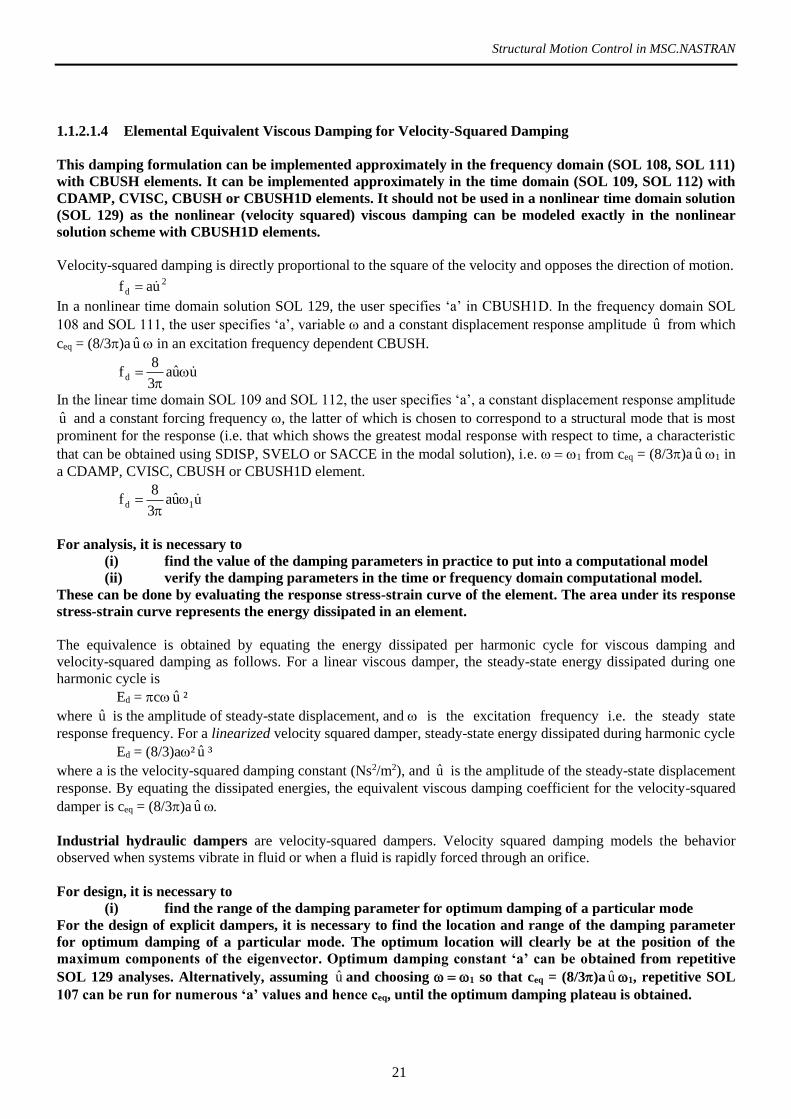
1.1.2.1.4 Elemental Equivalent Viscous Damping for Velocity-Squared Damping
This damping formulation can be implemented approximately in the frequency domain (SOL 108, SOL 111)
with CBUSH elements. It can be implemented approximately in the time domain (SOL 109, SOL 112) with
CDAMP, CVISC, CBUSH or CBUSH1D elements. It should not be used in a nonlinear time domain solution
(SOL 129) as the nonlinear (velocity squared) viscous damping can be modeled exactly in the nonlinear
solution scheme with CBUSH1D elements.
Velocity-squared damping is directly proportional to the square of the velocity and opposes the direction of motion.
2d uaf
In a nonlinear time domain solution SOL 129, the user specifies ‘a’ in CBUSH1D. In the frequency domain SOL
108 and SOL 111, the user specifies ‘a’, variable and a constant displacement response amplitude u from which
ceq = (8/3)a u in an excitation frequency dependent CBUSH.
uua3
8fd
In the linear time domain SOL 109 and SOL 112, the user specifies ‘a’, a constant displacement response amplitude
u and a constant forcing frequency , the latter of which is chosen to correspond to a structural mode that is most
prominent for the response (i.e. that which shows the greatest modal response with respect to time, a characteristic
that can be obtained using SDISP, SVELO or SACCE in the modal solution), i.e. 1 from ceq = (8/3)a u 1 in
a CDAMP, CVISC, CBUSH or CBUSH1D element.
uua3
8f 1d
For analysis, it is necessary to
(i) find the value of the damping parameters in practice to put into a computational model
(ii) verify the damping parameters in the time or frequency domain computational model.
These can be done by evaluating the response stress-strain curve of the element. The area under its response
stress-strain curve represents the energy dissipated in an element.
The equivalence is obtained by equating the energy dissipated per harmonic cycle for viscous damping and
velocity-squared damping as follows. For a linear viscous damper, the steady-state energy dissipated during one
harmonic cycle is
Ed = c u ²
where u is the amplitude of steady-state displacement, and is the excitation frequency i.e. the steady state
response frequency. For a linearized velocity squared damper, steady-state energy dissipated during harmonic cycle
Ed = (8/3)a² u ³
where a is the velocity-squared damping constant (Ns2/m2), and u is the amplitude of the steady-state displacement
response. By equating the dissipated energies, the equivalent viscous damping coefficient for the velocity-squared
damper is ceq = (8/3)a u
Industrial hydraulic dampers are velocity-squared dampers. Velocity squared damping models the behavior
observed when systems vibrate in fluid or when a fluid is rapidly forced through an orifice.
For design, it is necessary to
(i) find the range of the damping parameter for optimum damping of a particular mode
For the design of explicit dampers, it is necessary to find the location and range of the damping parameter
for optimum damping of a particular mode. The optimum location will clearly be at the position of the
maximum components of the eigenvector. Optimum damping constant ‘a’ can be obtained from repetitive
SOL 129 analyses. Alternatively, assuming u and choosing 1 so that ceq = (8/3)a u 1, repetitive SOL
107 can be run for numerous ‘a’ values and hence ceq, until the optimum damping plateau is obtained.

Structural Motion Control in MSC.NASTRAN
22
1.1.2.1.5 Elemental Equivalent Viscous Damping for Coulomb Damping
This damping formulation can be implemented approximately in the frequency domain (SOL 108, SOL 111)
with CBUSH elements. It can be implemented approximately in the time domain (SOL 109, SOL 112) with
CDAMP, CVISC, CBUSH or CBUSH1D elements. It should not be used in a nonlinear time domain solution
(SOL 129) as the damping can be modeled exactly in the nonlinear solution scheme with the CGAP (contact
and) friction element.
It is assumed that the (constant and limited) force resisting the direction of motion is proportional to the normal
force FN between the sliding surfaces, independent of the magnitude of velocity but is in phase with the velocity
(hence the sign of velocity term).
where F is the limiting Coulomb force magnitude and is equal to FN where FN is the normal contact force and
the coefficient of friction. In a nonlinear time domain solution SOL 129, the user specifies the coefficient of
friction, in a CGAP contact-friction element. In the frequency domain SOL 108 and SOL 111, the user specifies
, FN, variable and variable u from which c is calculated from ceq = FN/( u ). Due to the nature of the
Coulomb force being in phase with the velocity, an equivalent viscous damping model can easily be used in a
CBUSH element.
uu
F4f N
d
where FN is the normal force, the coefficient of friction and u the harmonic response amplitude. In the linear
time domain SOL 109 and SOL 112, a constant displacement response u and forcing frequency is required, the
latter of which is chosen to correspond to a structural mode that is most prominent for the response (i.e. that which
shows the greatest modal response with respect to time, a characteristic that can be obtained using SDISP, SVELO
or SACCE in the modal solution), i.e. 1. In the time domain, the user specifies , FN, 1 and u from which
ceq = FN/(1 u ) in a CDAMP, CVISC, CBUSH or CBUSH1D element.
uu
F4f N
d
For analysis, it is necessary to
(i) find the value of the damping parameters in practice to put into a computational model
(ii) verify the damping parameters in the time or frequency domain computational model.
These can be done by evaluating the response stress-strain curve of the element. The area under its response
stress-strain curve represents the energy dissipated in an element.
The energy dissipated is proportional to the friction force and the amplitude of vibration as follows.
Ed = 4FN u
Coulomb damping or dry friction damping is found wherever sliding friction is found in machinery, laminated
springs or bearings. Coulomb damping is also used to model joint damping mechanisms. Joint damping is found
in highly assembled structures.

Structural Motion Control in MSC.NASTRAN
23
1.1.2.1.6 Elemental Equivalent Structural Damping for Hysteretic Damping
This damping formulation can be implemented ONLY in the frequency domain (SOL 108, SOL 111) on the
MAT1 card or using CELAS or CBUSH elements. It will damp all the structural modes of vibration
accurately (obviously some modes will be damped more than others) for all excitation frequencies
irrespective of whether they are at resonance with the mode or not. It should not be used in a nonlinear time
domain solution (SOL 129) as the damping can be modeled exactly in the nonlinear solution scheme with an
elastic-plastic hysteretic material model MATS1 (TYPE PLASTIC).
The form of the damping force-deformation relationship depends on the stress-strain relationship for the material
and the make-up of the device. For an elastic-perfectly plastic material, the limiting values are Fy, the yield force,
and uy, the displacement at which the material starts to yield; kh is the elastic damper stiffness. The ratio of the
maximum displacement to the yield displacement is referred to as the ductility ratio and is denoted by . In a
nonlinear time domain solution SOL 129, the user specifies the initial stiffness kh, the yield force Fy and the
ductility ratio or the ultimate strain in a MATS1 (TYPE PLASTIC). In the frequency domain SOL 108 and SOL
111, the user specifies the equivalent structural damping loss factor GE for the hysteretic damper as
GE = 2(1)
where is the ductility ratio in a MAT1, CELAS or CBUSH element.
For analysis, it is necessary to
(i) find the value of the damping parameters in practice to put into a computational model
(ii) verify the damping parameters in the time or frequency domain computational model.
These can be done by evaluating the response stress-strain curve of the element. The area under its response
stress-strain curve represents the energy dissipated in an element.
The work per cycle for hysteretic damping is
Hysteretic damping is due to the inelastic deformation of the material composing the device. Hysteretic damping
is also offered by hysteretic damper brace elements.
For design, it is necessary to
(i) find the range of the damping parameter for optimum damping of a particular mode
For the design of explicit hysteretic damper brace elements, it is necessary to find the location and range of
the damping parameter for optimum damping of a particular mode. The optimum location will clearly be at
the position of the maximum components of the eigenvector. Optimum ductility ratio can be obtained from
repetitive SOL 129 analyses. Alternatively, assuming repetitive SOL 107 can be run for numerous GE values
and hence , until the optimum damping plateau is obtained.

Structural Motion Control in MSC.NASTRAN
24
1.1.2.1.7 Elemental Equivalent Structural Damping for Viscoelastic Damping
This damping formulation can be implemented ONLY in the frequency domain (SOL 108, SOL 111) on the
CBUSH elements or in SOL 108 with MAT1 and TABLEDi (with the SDAMPING Case Control Card). It
should not be used in a nonlinear time domain solution (SOL 129) as the damping can be modeled exactly in
the nonlinear solution scheme with the CREEP material model.
Viscoelastic materials are characterized by the shear modulus G (which relates to a stiffness k) and the loss factor,
GE both of which are temperature, strain and frequency dependent.
The ratio
is the shear loss tangent. A material is considered to be elastic when the stresses due to an excitation are unique
functions of the associated deformation i.e. = Ge. Similarly, a material is said to be viscous when the stress state
depends only on the deformation rates i.e. = Gv .
An elastic material responds in phase with excitation whilst a viscous element responds 90 degrees out of phase.
Hence a viscoelastic element responds 0 – 90 degrees out of phase with the excitation. In the frequency domain
SOL 108 and SOL 111, the user specifies the excitation frequency dependent stiffness, k() and the excitation
frequency dependent loss factor, GE() in a CBUSH element. Alternatively in SOL 108,
SDAMPING = n to reference TABLEDi Bulk Data entry
MAT1 with G = GREF (reference modulus) and GE = gREF (reference element damping)
A TABLEDi Bulk Data entry with an ID = n is used to define the function TR(f)
A TABLEDi Bulk Data entry with an ID = n+1 is used to define the function TI(f)
where the stiffness matrix of the viscoelastic elements
For analysis, it is necessary to
(i) find the value of the damping parameters in practice to put into a computational model
(ii) verify the damping parameters in the time or frequency domain computational model.
These can be done by evaluating the response stress-strain curve of the element. The area under its response
stress-strain curve represents the energy dissipated in an element.

Structural Motion Control in MSC.NASTRAN
25
Viscoelastic damping is present in most materials, albeit at very small levels. This is of course present in both the
elastic and plastic range of the material deformation and their values are presented below.
Material Loss Factor, GE
Steel 0.001 – 0.008
Cast iron 0.003 – 0.03
Aluminium 0.00002 – 0.002
Lead 0.008 – 0.014
Rubber 0.1 – 0.3
Glass 0.0006 – 0.002
Concrete 0.01 – 0.06
Viscoelastic damping is utilized in constrained layer damping for structural and aeronautical applications.
Examples include SUMITOMO-3M, SWEDAC and bituthene. This method works best when the constrained layer
is put into shear and therefore the most effective location of such a layer is at the neutral axis of the floor beam or
slab where the complementary shear stresses are high. Typical visco-elastic materials are fairly flexible and can
exhibit significant creep. Therefore introduction of a constrained layer means that the structure is more flexible
than it would be if it were monolithic. For static loads therefore these types of layers are not ideal, and so a
compromise must often be reached. Constrained layer damping has quite often been applied to excessively lively
existing structures by adding an extra “cover plate” on top of or beneath the existing floor in order to constrain a
layer of visco-elastic material.
The stiffness k of a (zero-length two orthogonal horizontal direction) spring representing an area A of viscoelastic
constrained layer material is AG/t where t is the thickness and G the shear modulus. The variation of G and the loss
factor GE with temperature, excitation frequency has been established for bituthene.
Temperature has dramatic effect on G but little on GE. The material properties to use based on interpolation of test
results at 20 C and a frequency of 5Hz are thus
Shear Modulus G = 1.17 MPa
Loss factor GE = 0.75 (at very small strains)
For design, it is necessary to
(i) find the range of the damping parameter for optimum damping of a particular mode
Optimum damping parameters k and GE can be obtained from repetitive SOL 107 analyses, until the
optimum damping plateau is obtained. For constrained layer viscoelastic damping, repetitive SOL 107 can
be run until the value of k (and hence the thickness t since k = AG/t) that yields the optimum damping is
obtained.
Slab
Truss end

Structural Motion Control in MSC.NASTRAN
26
1.1.2.2 Modal Damping Mathematical Models
Modal damping damps all the structural modes of vibration specified with a modal damping accurately at
all excitation frequencies irrespective of whether they are at resonance with the mode or not. Equivalent
modal damping damps the structural modes of vibration specified with a modal damping accurately ONLY
when the excitation frequency matches the frequency of each particular natural mode.
Note that the modal damping approach will not be valid if the modes are significantly complex, i.e. different parts
of the structure are out-of-phase (reaching their maximum at different instances) in a particular mode as the modal
damping values are applied on the real modes. Damping elements with high values of damping can result in the
structure having totally different damped modes of vibration. For instance, a cable with a damper element with a
very high damping coefficient attached to its center will behave as two separate cables, the damper element
effectively producing a fixity at the center of the cable. This changes the fundamental mode shape of the cable from
one of a low frequency to two cable mode shapes of higher fundamental frequency.
For analysis, it is necessary to
(i) find the value of the damping parameters in practice to put into a computational model
(ii) obtain modal damping values from a set of explicit element dampers
There are various methods of obtaining the modal damping coefficients in practice and from finite element models
damped with individual explicit viscous or structural damping elements. Complex modal analysis (SOL 107) can
be performed to ascertain the structural modal damping coefficients Gi for each and every mode. Alternatively, a
forced frequency response analysis (SOL 108 or SOL 111) can be performed with a harmonic loading from
which the modal damping coefficient can be ascertained in a variety of methods from the FRF. The methods of
obtaining the damping from the FRF are: -
(i) the half-power bandwidth method which approximates the modal damping in lightly-damped structures (
< 0.1) where the ith modal damping coefficient is
where fi1 and fi2 are the beginning and ending frequencies of the half-power bandwidth defined by the
maximum response divided by 2. The half-power bandwidth method assumes a SDOF response.
(ii) the (magnitude of the) dynamic amplification factor at resonance method
Another method of obtaining modal damping estimates is the logarithmic decrement method. In order to obtain
the values of i, a transient analysis (SOL 109, SOL 112, SOL 129) can be performed and successive peaks can be
observed from the free vibration response. The free vibrational analysis can be set up using an initial displacement
condition or an impulsive force that ramp up and down quickly with respect to the dominant period of the response
and/or other natural frequencies of interest. The logarithmic decrement, is the natural log of the ratio of amplitude
of two successive cycles of free vibration. Then the damping ratio is
The logarithmic decrement method assumes a SDOF response. Modal damping of higher modes requires signal
filtering of the response time history.
/kp Amplitude, Responsent Displaceme Static
/kpD mode,ith of Amplitude Responsent Displaceme Maximum
D mode,ith of ResonanceAt Factor ion Amplificat Dynamic2
1
0
0resonant i
resonant i
i
i
1i2ii
f2
ff
2

Structural Motion Control in MSC.NASTRAN
27
1.1.2.2.1 Modal Viscous Damping
This damping formulation can be implemented in the modal time domain (SOL 112) with the SDAMPING
Case Control Command and the TABDMP1 entry. It can also be implemented in the modal frequency
domain (SOL 111) with SDAMPING Case Control Command, the PARAM, KDAMP and the TABDMP1
entry. It will damp all the structural modes of vibration specified with a modal damping value accurately for
all excitation frequencies irrespective of whether they are at resonance with the mode or not.
The damping force is given by
The user specifies i.
1.1.2.2.2 Modal Structural Damping
This damping formulation cannot be implemented in the modal time domain (SOL 112). It can be
implemented in the modal frequency domain (SOL 111) with the SDAMPING Case Control Command, the
PARAM, KDAMP and the TABDMP1 entry where it will damp all the structural modes of vibration
specified with a modal damping value accurately for all excitation frequencies irrespective of whether they
are at resonance with the mode or not.
The damping force is given by
The user specifies Gi.
1.1.2.2.3 Modal Equivalent Viscous Damping for Modal Structural Damping
There no reason to implement this damping formulation in the modal frequency domain as modal structural
damping can be specified instead. It can be implemented in the modal time domain (SOL 112) with the
SDAMPING Case Control Command and the TABDMP1 entry. This damping formulation will damp all
modes specified with a modal damping value accurately ONLY when the excitation frequency matches the
natural frequency of the particular mode (i.e. at resonance), often an acceptable approximation.
This modal damping formulation is extremely useful in modelling structural damping in time domain solutions.
Time domain solutions, be they direct or modal cannot handle structural damping. Incorporating elemental
structural damping within a time domain solution requires a ‘tie in’ frequency, hence damping the different modes
inaccurately. The best method would be to use a modal approach, i.e. SOL 112 where modal damping can be
specified and internally automatically converted into modal viscous damping. All the modes are then damped
accurately when the excitation frequency matches the natural frequency of the particular mode. Again, the method
works if the modes are only slightly complex, as the modal damping estimates are applied onto the real modes.
The following presents the appropriate conversion between modal viscous and modal structural damping. It will be
shown that the two forms of damping are only theoretically equivalent when the forcing frequency equals the
natural frequency of the structural mode of vibration n. This is proven mathematically and pictorially below
showing the variation of viscous and structural damping with forcing frequency.
))((i )2(f iiniid iM
)(iGf iiid iK

Structural Motion Control in MSC.NASTRAN
28
For the viscous damping force to equal the structural damping force
The damping constant c is specified as a percentage of critical damping of a particular structural mode
i(2mn)u = iGku
(2mn) = Gk
If and only if = n
n(2mn) = Gk
2mn2 = Gk
2mk / m = Gk
= G / 2
Although the two damping formulations are only identical the resonances = n and not for other forcing
frequencies, damping is most critical at resonance when n (when the inertial and stiffness forces cancel) and
so the switch between viscous and structural formulations is often acceptable in practice. Whenever possible, the
damping formulation chosen (i.e. whether viscous or structural) should be such as to simulate the actual real-world
damping mechanism. Nevertheless, the use of viscous damping to simulate structural damping (and vice versa for
that matter) is possible, but it must be borne in mind that the conversion is only accurate at resonance when the
structural modal frequencies equal the forcing frequencies. From above, it is obvious that the use of a viscous
damping formulation to represent a structural damping mechanism will overestimate damping when the forcing
frequency is higher than ni and underestimate damping when the forcing frequency is lower than ni.
Conversely, the use of a structural damping formulation to represent a viscous damping mechanism will
underestimate damping when the forcing frequency is higher than ni and overestimate damping when the
forcing frequency is lower than ni.
Structural
damping
Viscous
damping
fd
Forcing
frequency, = n
iGkuuic
iGkuuc
ff structuralviscous
Structural Motion Control in MSC.NASTRAN
29
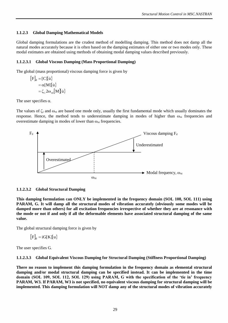
1.1.2.3 Global Damping Mathematical Models
Global damping formulations are the crudest method of modelling damping. This method does not damp all the
natural modes accurately because it is often based on the damping estimates of either one or two modes only. These
modal estimates are obtained using methods of obtaining modal damping values described previously.
1.1.2.3.1 Global Viscous Damping (Mass Proportional Damping)
The global (mass proportional) viscous damping force is given by
The user specifies
The values of i and ni are based one mode only, usually the first fundamental mode which usually dominates the
response. Hence, the method tends to underestimate damping in modes of higher than ni frequencies and
overestimate damping in modes of lower than ni frequencies.
1.1.2.3.2 Global Structural Damping
This damping formulation can ONLY be implemented in the frequency domain (SOL 108, SOL 111) using
PARAM, G. It will damp all the structural modes of vibration accurately (obviously some modes will be
damped more than others) for all excitation frequencies irrespective of whether they are at resonance with
the mode or not if and only if all the deformable elements have associated structural damping of the same
value.
The global structural damping force is given by
The user specifies G
1.1.2.3.3 Global Equivalent Viscous Damping for Structural Damping (Stiffness Proportional Damping)
There no reason to implement this damping formulation in the frequency domain as elemental structural
damping and/or modal structural damping can be specified instead. It can be implemented in the time
domain (SOL 109, SOL 112, SOL 129) using PARAM, G with the specification of the ‘tie in’ frequency
PARAM, W3. If PARAM, W3 is not specified, no equivalent viscous damping for structural damping will be
implemented. This damping formulation will NOT damp any of the structural modes of vibration accurately
uM2
u]M[
u]C[F
nii
d
Viscous damping Fd Fd
Modal frequency, ni
ni
Underestimated
Overestimated
u]K[iGF d

Structural Motion Control in MSC.NASTRAN
30
except the solitary ‘tied in’ mode that will be damped accurately ONLY when the excitation frequency
matches its natural frequency (i.e. at resonance). Hence, this damping formulation should NOT be used, a
modal approach should be used for the time domain instead.
The global (stiffness proportional) viscous damping force is given by
The user specifies
The values of i and ni are based one mode only, usually the first fundamental mode which usually dominates the
response. Hence, the method tends to overestimate damping in modes of higher than ni frequencies and
underestimate damping in modes of lower than ni frequencies.
This method is crudely used to model the structural damping mechanism in a global viscous formulation. This is so
because, from the above equation
As mentioned, a viscous formulation to model structural damping will overestimate damping when the forcing
frequency is higher than ni and underestimate damping when the forcing frequency is lower than ni. This is
even more exaggerated here as the damping estimate is based upon just one mode.
1.1.2.3.4 Global Equivalent Viscous Damping for Viscous and Structural Damping (Mass and Stiffness
Proportional Rayleigh Damping)
The Rayleigh proportional viscous damping force is given by
The user specifies and
uK2
u]K[F
ni
i
d
u]K[iG
u]K[2iF
When
iuK2
u]K[F
i
id
ni
ni
i
d
Viscous damping Fd
Fd
Modal frequency, ni
ni
Underestimated
Overestimated
u]K[]M[F d

Structural Motion Control in MSC.NASTRAN
31
The factors and are chosen to give the correct damping at two excitation frequencies. For a specified damping
factor at an excitation frequency then
And using this at 2 frequencies r and s with the required damping factors r and s respectively gives
The method is based on the damping coefficients r and s of two distinct modes r and s. By specifying r = s,
all structural natural modes between modal frequencies r and s will have damping less than at modes r and s.
1.1.2.4 Damping Formulation Conclusions
The choice of using a viscous damping formulation or a structural damping formulation should depend on the
actual real world damping mechanism being modeled. Elemental damping formulations damp all modes accurately
at all excitation frequencies. If an equivalent elemental damping formulation is used, then not all natural modes will
be damped accurately. Modal damping formulations damp all modes specified with a modal damping accurately at
all excitation frequencies. Equivalent modal damping formulations damp all modes specified only when the
excitation frequency matches the natural frequency of the mode. The use of a modal viscous damping formulation
to represent a modal structural damping mechanism will overestimate the modal damping when the forcing
frequency is higher than ni and underestimate the modal damping when the forcing frequency is lower than
ni. Conversely, the use of a modal structural damping formulation to represent a modal viscous damping
mechanism will underestimate the modal damping when the forcing frequency is higher than ni and
overestimate the modal damping when the forcing frequency is lower than ni. Global proportional damping will
damp only one or two structural modes accurately. Global mass proportional viscous damping tends to
underestimate damping in modes of higher than ni frequencies and overestimate damping in modes of lower than
ni frequencies. Global structural damping will damp all modes accurately at all excitation frequencies if all the
deformable elements exhibit structural damping of the same value. Global stiffness proportional viscous damping
tends to overestimate damping in modes of higher than ni frequencies and underestimate damping in modes of
lower than ni frequencies. Global Rayleigh damping can be made, by specifying r = s, to damp all modes
between modal frequencies r and s to have damping less than at modes r and s.
2s
2r
ssrr
2s
2r
srrssr
2
2
Modal frequency, n
Viscous damping Fd
Fd
r s
2
1

Structural Motion Control in MSC.NASTRAN
32
1.1.3 GL, ML Base Isolation Systems
Base isolation systems are used to minimize the effect of seismic support motion on structures and
nonstructural elements and to reduce machine induced loadings on foundations.
1.1.3.1 Controlling Displacement Response From Harmonic Load Excitations
We reiterate that the dynamic amplification factor D() for applied harmonic loading p0sint on a SDOF system is
The corresponding maximum displacement response of the SDOF system is umax = Dimax(p0/k). Dimax occurs when
/n = (1-22)1/2. Clearly, if n is flexible (i.e. low) enough such that D() is less than unity (the exact location
varies with the amount of damping, being at /n = 1.4 for = 0.0), the steady-state dynamic response will be less
than the static response and the externally applied harmonic dynamic load excitation is well controlled for the
displacement response.
1.1.3.2 Controlling Acceleration Response From Harmonic Load Excitations
Now, it may also be desirable to limit the maximum acceleration amplitude. The acceleration response is simply
the second derivative (with respect to time) of the displacement response. Hence the maximum acceleration
response will be amax = 2Dimax(p0/k) = (/n)2Dimax(p0/m).
Variation of ( /n)^2.D() with
Frequency Ratio For Different Damping
0
1
2
3
4
5
6
7
0 1 2 3
Frequency Ratio /n
( /
n)^
2.D
( )
zhi=0
zhi=0.1
zhi=0.2
zhi=1
zhi=2
2maxi
2
nii
22
ni2
i
12
1D
;
/2/1
1)(D
2
maxi
2
ni
2
nii
22
ni2
2
nii
2
ni
12
1D/
;
/2/1
/)(D/
Variation of D with Frequency Ratio For Different
Damping
0
1
2
3
4
5
6
0 1 2
Frequency Ratio /n
Dy
nam
ic A
mp
lifi
ca
tion
Facto
r,
D
zhi=0
zhi=0.1
zhi=0.2
zhi=1
zhi=2

Structural Motion Control in MSC.NASTRAN
33
2
n22
n2
2
n
r
)/2()1(
/21T
Note that the behaviour of (/n)2Di() for small and large /n is opposite to that of Di(). The maximum is the
same but the location is different. The ratio p0/m is the acceleration of the mass if the mass is unrestrained. Hence
(/n)2Di() approaches unity for large (/n)2. The term (/n)2Di() is then the multiplier to p0/k accounting for
the time varying nature of the loading and the stiffness and damping of the system. Clearly, /n needs to be such
that (/n)2Di()p0/m is within the acceptable acceleration limit.
1.1.3.3 Base Isolation - Controlling Displacement Response From Harmonic Base Enforced Motion
For a SDOF system subjected to base harmonic excitations u0sint, in absolute terms the response would be
Defining an expression for the displacement transmissibility as the absolute displacement response amplitude
divided by the amplitude of the enforcing harmonic displacement u0,
This is the (absolute) displacement transmissibility expression.
When we design for the displacement response, it is usually the relative response that we are concerned with. Now
the steady state solution for the relative (to base) displacement is
This expression is numerically equivalent to (/n)2Di() and is shown below.
Clearly for design,/n needs to be such that (/n)2Di()u0 is within the acceptable relative displacement limit.
Note that for large /n values the expression approaches unity and hence the relative displacement response
approaches the displacement of the base motion and needs to be designed for.
Variation of ( /n)^2.D() with
Frequency Ratio For Different Damping
0
1
2
3
4
5
6
7
0 1 2 3
Frequency Ratio /n
( /
n)^
2.D
( )
zhi=0
zhi=0.1
zhi=0.2
zhi=1
zhi=2
)/2(tan
)1(
/2tantsin
)/2()1(
/21u)t(u n
1
2n
2
n1
2n
22n
2
2
n0
)1(
/2tantsin
)/2()1(
/u)t(u
2n
2
n1
2n
22n
2
2n
20
r

Structural Motion Control in MSC.NASTRAN
34
2
n22
n2
2
n
r
)/2()1(
/21T
1.1.3.4 Base Isolation - Controlling Acceleration Response From Harmonic Base Enforced Motion
The acceleration transmissibility (absolute acceleration response amplitude divided by the amplitude of the
enforcing harmonic acceleration) is exactly similar to the (absolute) displacement transmissibility.
This formula is effective to determine the natural frequency (hence stiffness) and damping of an isolation system
knowing the input displacement or acceleration and the maximum acceptable dynamic acceleration that the
structural component can be subjected to.
Remember that only when damping is small that the maximum transmissibility can be approximated to occur at
resonance. When damping is high, it is imperative that the transmissibility expression be differentiated or plotted
(also use cannot be made of = n(1-22)1/2 as this is based on differentiating and maximizing the (magnitude of
the) dynamic amplification factor, D()).
A plot of Tr versus /n is somewhat similar to that of (magnitude of the) dynamic amplification D versus /n,
except that all the curves of different pass through the same point of Tr = 1.0 when /n = 2. Noting the curves
after this point it is observed that damping tends to reduce the effectiveness of vibration isolation for frequency
ratios greater than 2.
On investigating the transmissibility expression, we can design the supporting system for vibration isolation. The
transmissibility is unity when the supporting system is infinitely stiff with respect to the loading frequency. The
transmissibility is also unity when the frequency ratio is 2. If the supporting system is designed such that the
frequency ratio is less than 2 but greater than 0, the transmissibility is greater than one, which means that the
supporting system actually makes matters worse as far as vibration isolation is concerned. When the frequency
ratio is greater than 2, it is seen that the transmissibility is smaller than unity and hence, the supporting system
functions as a vibration isolator. Damping is seen to be advantages only in the region when the frequency ratio is
less than 2 (where a spring mounting supporting system makes matters worse) and not when the frequency ratio is
greater than 2 (where a spring mounting supporting system acts as a effective vibration isolator). This is not so
important actually as the undesirable effects of high values of damping at frequency ratios greater than 2 is not so
great especially at even higher frequency ratios, i.e. achieved by making the supporting system even more flexible.
0
1
2
3
4
5
6
0 1 2
Tra
nsm
issib
ilit
y,
Tr
Frequency Ratio /n
Variation of Tr with Frequency Ratio For Different Damping
zhi=0
zhi=0.1
zhi=0.2
zhi=0.3
zhi=0.4
zhi=1.0
zhi=2.0

Structural Motion Control in MSC.NASTRAN
35
Also, in the unfortunate circumstance that the resonance region of frequency ratio less than 2 is somehow
attained; high levels of damping are extremely effective. For good isolation, it is often recommended to design the
supporting system for a frequency ratio of at least 3.
An example of isolation systems in practice occurs in the case of the EUROSTAR train.
Bogie 1 Typical Bogie Bogie 9
M tonne 40.021 27.000 32.102
Ks kN/m 870 580 1250
Cs kNs/m 20 2 20
Mb tonne 3.025 3.250 3.200
Ib tm² 2.800 2.800 2.800
Kp kN/m 2200 2075 1560
Cp kNs/m 12 12 12
a m 3.0 3.0 3.0
Mw tonne 2.128 2.095 2.113
The primary (bogie) suspension system has a natural frequency of about 5.7Hz, hence filtering frequencies higher
than 2 x 5.7 = 8.1Hz. The secondary (deck) suspension system has a natural frequency of about 0.7Hz, hence
filtering frequencies higher than 2 x 0.7 = 1.0Hz.

Structural Motion Control in MSC.NASTRAN
36
2
n22
n2
2
n
r
)/2()1(
/21T
Below is the modulus FFT of the acceleration response showing clearly the dominant frequency components of the
response at the wheels, bogie and train deck.
Another reason to employ isolation is to isolate rail-induced vibrations through the ground onto submerged
structures or adjacent structures. The frequency content ranges from 1Hz to 150-200Hz. Structural vibrations occur
due the 8Hz to 20Hz frequencies. Railway excitations have a pronounced frequency band between 40Hz and 80Hz,
causing significant acoustic phenomena (structure borne sound). Note that noise can be detected above a frequency
of about 16Hz. Vibration isolation devices typically ranging from 8Hz to 12Hz can be used to isolate frequencies
above these.
Road traffic also induces vibration with a frequency range from 1 to 200-400Hz but does not, in contrast with rail-
induced vibrations, exhibit pronounced frequency components.
1.1.3.5 Base Isolation – Controlling Force Transmitted Into Foundation From Harmonic Load Excitations
The force transmissibility (force response amplitude divided by the amplitude of the enforcing harmonic force of
p0sint, i.e. p0) is also exactly similar to the (absolute) displacement transmissibility.
The transmissibility expression can be used for the force induced by a rotating machine into the supporting
structure. Design supporting system such that /n = 2 for no dynamic effects. Note that the transmissibility
expression is only valid for the force transmitted if the foundation is rigid. If the foundation is not rigid, then the
supporting system must be even more flexible in order to provide the same level of protection as when the
foundation is rigid.

Structural Motion Control in MSC.NASTRAN
37
1.1.4 GL, ML Tuned Mass Damper (TMD) Systems
The TMD is a device consisting of a mass, spring and damper to reduce mechanical vibrations. The frequency and
damping of the TMD is tuned so that when the structure resonates at a particular frequency, the TMD vibrates out-
of-phase transferring the energy from the primary system (i.e. the structure) to the secondary system (i.e. the TMD)
and dissipating it in the damper. Maximum flow of energy from the primary system to the TMD occurs when the
displacement of the TMD lags that of the primary mass by 90°. The acceleration of the TMD is then in phase with
velocity of the primary system.
The TMD concept was introduced by Frahm in 1909 to reduce the rolling motion of ships and ship hull vibrations.
Significant theoretical contributions were made by Den Hartog (1940) for undamped systems subject to harmonic
excitations. Extensions to the theory were then presented by Randall (1981), Warburton (1982) and Tsai & Lin
(1993).
The figure below illustrates the typical configuration of a unidirectional translational tuned mass damper. The mass
rests on bearings that function as rollers and allow the mass to translate laterally relative to the floor. Springs and
dampers are inserted between the mass and the adjacent vertical support members which transmit the lateral “out-
of-phase” force to the floor level, and then into the structural frame. Bidirectional translational dampers are
configured with springs/dampers in 2 orthogonal directions and provide the capability for controlling structural
motion in 2 orthogonal planes.
The early versions of TMD’s employ complex mechanisms for the bearing and damping elements, have relatively
large masses, occupy considerably space, and are quite expensive. Recent versions, such as the scheme shown
below, have been designed to minimize these limitations. This scheme employs a multi-assemblage of elastomeric
rubber bearings, which function as shear springs, and bitumen rubber compound (BRC) elements, which provide
viscoelastic damping capability. The device is compact in size, requires unsophisticated controls, is
multidirectional, and is easily assembled and modified.

Structural Motion Control in MSC.NASTRAN
38
The problems associated with the bearings can be eliminated by supporting the mass with cables which allow the
system to behave as a pendulum.
The equation of motion for the horizontal direction is
where T is the tension in the cable. When is small, the following approximations apply
Hence
and it follows that the equivalent shear spring stiffness is
The natural frequency of the pendulum is
The natural period of the pendulum is
The simple pendulum tuned mass damper concept has a serious limitation. Since the period depends on L, the
required length for large Td may be greater than the typical story height. This problem can be eliminated by
resorting to the scheme illustrated below.

Structural Motion Control in MSC.NASTRAN
39
The interior rigid link magnifies the support motion for the pendulum, and results in the following equilibrium
equation.
The rigid link moves in phase with the damper, and has the same displacement amplitude. Then, taking u1= ud
The equivalent stiffness is Wd/2L, and it follows that the effective length is equal to 2L. Each additional link
increases the effective length by L.
The concepts of designing the passive tuned mass damper illustrated below are based on geometrically and
materially linear frequency domain dynamic analyses. In deriving the equations of motion, we use absolute terms
of displacement, velocity and acceleration unless we have support motion, in which case it is easier to use relative
terms. Note that in absolute terms, we need the support displacement and velocity in the equation of motion whilst
in relative terms we need only the support acceleration in the equation of motion.

Structural Motion Control in MSC.NASTRAN
40
)1(
/2tan),tcos(
/2/1
k/map)t(u
e)(F alRe)t(u
issolution state-steady theThus,
/1
/2tan,e
/2/1
k/map)(F
/1
/2tan
mk
ctan,
ecmk
map)(F
icmk
map)(F
map)(kF)(Fic)(Fm
,e)(F alRe)t(u assume solution), state-(steadypart usinhomogeno For the
ea alRe)t(uandep alRe)t(P
s,excitation harmonic For
)t(um)t(P)t(ku)t(uc)t(um
)t(P)t(ku)t(uc)t(u)t(um
,Hence
)t(u)t(u)t(u
terms,relative In
)t(P)t(u)t(uk)t(u)t(uc)t(um
ismotion support and excitation force harmonic tosubjected system SDOF a ofmotion ofequation the terms,absoluteIn
2n
2
n1
2
n
22
n2
00r
tir
2
n2
n1i
2
n
22
n2
00
2
n2
n1
2
1
i222
00
2
00
002
tir
ti0s
ti0
srrr
rrsr
sr
ss
1.1.4.1 Damped SDOF System Subject to Harmonic Force and Support Motion Excitations
The analysis of the TMD involves the prediction of the response of a two-DOF system, the first being that of the
primary system and the second being the TMD. Extensive use is made of (complex arithmetic) mathematical
procedures to predict the steady-state response due to harmonic excitations in the frequency domain. The
employment of complex arithmetic simply allows the representation of the response and the excitation functions in
complex numbers. To illustrate this elegant mathematical approach, the steady-state response of a SDOF system is
first illustrated, forming the basis of further analyses involving the TMD and the primary system.
u(t)
m
k
P(t) = p0cost
cd
tcosa )t(u 0s

Structural Motion Control in MSC.NASTRAN
41
ti
dd
ti
d
n
dd
n
d
i
22222
20
d
i
22222
220
d
dddd2
d
0ddd2
tidd
ti
ti0
dddd
dd
e)(F alRe)t(u
e)(F alRe)t(u
are solutions state-steady the,completionFor
m
mratio mass
m/kratiofrequency forced
m/k
m/kratiofrequency naturalf
thatNote
eff1k
p)(F
eff1
f
k
p)(F
yield, toformpolar into converted and )(F and )(F
(FRFs) functions responsefrequency complex for theusly simultaneo solved becan which equations twoare These
0)(Fk)(Fk)(Fm
p)(Fk)(Fk)(kF)(Fm
,e)(F alRe)t(u and e)(F alRe)t(u assume solution), state-(steadypart usinhomogeno For the
ep alRe)t(P
s,excitation harmonic For
0)t(u)t(uk)t(um
)t(P)t(u)t(uk)t(ku)t(um
are excitation force harmonic tosubjected system DOF two theofmotion of equations the terms,absoluteIn
2
1
1.1.4.2 Undamped Structure, Undamped TMD System Subject to Harmonic Force Excitation
Note that n2 = k / m
d2 = kd / md
The plot of the magnitude of the FRF F() (of the primary system) divided by the static displacement p/k, i.e. the
(magnitude of the) dynamic amplification factor D() is presented.
u(t)
m
k
P(t) = p0cost
ud(t)
md
kd

Structural Motion Control in MSC.NASTRAN
42
The optimum conditions are ascertained by changing the mass ratio and the natural frequency ratio f.
Changing the frequency ratio, f has the effect of changing the position where D() becomes zero, i.e. D()
becomes zero at when = f. Changing the mass ratio has the effect of changing the distance between the peaks of
D() with higher values resulting in a greater spread.
Dynamic Magnification Factor of Primary System D(w)
0
2
4
6
8
10
12
14
16
18
20
0.6 0.8 1 1.2
Forcing Frequency Ratio,
D(w
)
Primary Mass Primary Mass - TMD (f = 1.0)
Primary Mass - TMD (f = 1.1)
Dynamic Magnification Factor of Primary System D(w)
0
2
4
6
8
10
12
14
16
18
20
0.6 0.8 1 1.2
Forcing Frequency Ratio,
D(w
)
Primary MassPrimary Mass - TMD (mass ratio = 0.1)Primary Mass - TMD (mass ratio = 0.2)

Structural Motion Control in MSC.NASTRAN
43
ti
dd
ti
d
n
dd
n
d
i
22d
222222
20
d
i
22d
222222
2
d
222
0
d
ddddddd2
d
0dddddd2
tidd
ti
ti0
dddddd
dddd
e)(F alRe)t(u
e)(F alRe)t(u
are solutions state-steady the,completionFor
m
mratio mass
m/kratiofrequency forced
m/k
m/kratiofrequency naturalf
thatNote
e
11f2ff1k
p)(F
e
11f2ff1
f2f
k
p)(F
yield, toformpolar into converted and )(F and )(F
(FRFs) functions responsefrequency complex for theusly simultaneo solved becan which equations twoare These
0)(Fk)(Fk)(Fic)(Fic)(Fm
p)(Fk)(Fk)(Fic)(Fic)(kF)(Fm
,e)(F alRe)t(u and e)(F alRe)t(u assume solution), state-(steadypart usinhomogeno For the
ep alRe)t(P
s,excitation harmonic For
0)t(u)t(uk)t(u)t(uc)t(um
)t(P)t(u)t(uk)t(u)t(uc)t(ku)t(um
are excitation force harmonic tosubjected system DOF two theofmotion of equations the terms,absoluteIn
2
1
1.1.4.3 Undamped Structure, Damped TMD System Subject to Harmonic Force Excitation
Note that n2 = k / m
d2 = kd / md
c = 2nm (here undefined)
cd = 2ddmd
u(t)
m
k
P(t) = p0cost
ud(t)
md
kd
cd

Structural Motion Control in MSC.NASTRAN
44
The plot of the magnitude of the FRF F() (of the primary system) divided by the static displacement p/k, i.e. the
(magnitude of the) dynamic amplification factor D() is presented.
The optimum conditions are ascertained by changing the mass ratio , the natural frequency ratio f and the level
of damping d. It is noticed that for whatever combination, there will always be two common points (which are
independent of d) on the plot of D().
The greater the mass ratio , the lower will be the response. Also, a larger mass ratio would render the TMD less
sensitive to tuning, a characteristic which is much valuable in practice as the estimate of the modal frequencies
change with insertion of cladding, non-structural components etc. The mass ratio is usually between 0.01 and 0.1.
By changing the ratio of the natural frequency ratio f, we will change the relative height of the two common points.
The optimum condition will be when the two common points are at the same height. It can be shown from algebra
that this condition is achieved when f is tuned such that
which gives the amplitude at the common points as
2
1D
By changing the damping d we will change the point at which the curves attain their maxima, i.e. whether at the
above common points or not. We know that the amplitude at resonance is limited only by the damping force. If d =
0, there is no energy dissipation and hence two (since this is a two-DOF system) resonant peaks of infinite
amplitude is attained on D(). When d is infinite, the two masses are practically locked to each other, their relative
displacement is thus zero, hence causing no work to be done by the damper, and thus a single resonant peak of
infinite amplitude is attained on D(). There is thus an optimum value of d for which there will be maximum work
done by the damper, and this would be the point at which the response of the primary system is minimum. The
Dynamic Magnification Factor of Primary System D(w)
0
2
4
6
8
10
12
14
16
18
20
0.6 0.8 1 1.2
Forcing Frequency Ratio,
D(w
)
Damping 0.0 of Critical Damping 0.1 of Critical
Damping 0.32 of Critical
Common Points
1
1fopt

Structural Motion Control in MSC.NASTRAN
45
optimum condition for the choice of d is achieved when the two curves pass the common points at the maxima.
But this does not occur at the same time. Expressions for when the first curve passes the first common point at its
maximum and the second curve passes the second common point at its maximum can be averaged to yield a useful
optimum damping of
Thus, in order to design a TMD to reduce vibrations from harmonic force excitations, the following approach is
undertaken. Clearly, one should select the TMD location to coincide with the maximum amplitude of the mode
shape that is being controlled.
(i) Choose the practically greatest possible mass ratio, whilst still satisfying the maximum displacement
criteria for both F() and Fd()
(ii) Determine the optimum natural frequency ratio, f and hence calculate the stiffness of the TMD, kd
(iii) Determine the optimum damping ratio, d,opt and hence calculate the optimum damping of the TMD, cd
As an example, we shall investigate the design of a TMD for the London Heathrow Terminal 5 Visual Control
Tower. The 85.5m high tower has a total mass of 680.9 tonnes and a fundamental global tower mode (0.91Hz)
modal mass of 396 tonnes with the eigenvector normalized at the location of the TMD, i.e. at 78.3m. Note that
there are other local (cable) modes of lower frequencies.
18
3opt,d
2ddd
noptd
opt
mk
f
1
1f
ddopt,dopt,d
opt,d
m2c
18
3

Structural Motion Control in MSC.NASTRAN
46
The natural frequencies of the modes of the tower are presented for completion. The corresponding modal masses
are also presented with the eigenvectors MAX normalized.
T5 VCR REAL MODAL ANALYSIS - MODAL MASS
0.000
25.000
50.000
75.000
100.000
125.000
150.000
175.000
200.000
225.000
250.000
0 5 10 15 20 25 30 35 40 45 50
Mode Number
Mod
al
Mass
(T
on
nes
)
Primary Tower
Bending Modes
Secondary Tower
Bending Modes
Cable Modes Cable Modes Cable ModesCable Modes
Primary Tower
Torsion Mode
T5 VCR REAL MODAL ANALYSIS - FREQUENCY
0.000
0.500
1.000
1.500
2.000
2.500
3.000
3.500
4.000
0 5 10 15 20 25 30 35 40 45 50
Mode Number
Freq
uen
cy (
Hz)
Primary Tower
Bending Modes
Secondary Tower
Bending Modes
Cable Modes
Cable Modes Cable Modes
Cable Modes
Primary Tower
Torsion Mode

Structural Motion Control in MSC.NASTRAN
47
The characteristic of the modes are also expounded.
The calculation for optimum properties of a 25 tonne TMD is presented.
Nat
ura
l F
requ
ency
(H
z)
Ns/m 103.41936
f2*25000*2
m2c t,Coefficien Damping Viscous
14922.0
)1(8
3 Ratio, Damping Optimum
N/m 14.789745
895.0*2*25000
f2mk TMD, of Stiffness Optimum
Hz 895.0
951.0*9406.0
fff System,Secondary of Frequency
9406.01
1f Ratio,Frequency Optimum
0631.0396000
25000
m
m Ratio, Mass
optd
optddd
opt
2
2
ddd
1optd
opt
d

Structural Motion Control in MSC.NASTRAN
48
The figure below shows the displacement magnification factor D() at the AMD level with harmonic excitation at
the AMD level. This shows that the effective damping of the primary tower mode from the TMD is 9.7% of critical
since the reduction of maximum amplification reduces from 33.2 to 4.84.

Structural Motion Control in MSC.NASTRAN
49
ti
ddr
tir
d
n
dd
n
d
i
22d
222222
0d
i
22d
222222
2
d
222
0
d
2d0dddddd
2d
0dddd2
tiddr
tir
ti0s
rdsddrddrddrd
sdrddrdrr
srdddr
sr
dddddd
dddds
e)(F alRe)t(u
e)(F alRe)t(u
are solutions state-steady the,completionFor
m
mratio mass
m/kratiofrequency forced
m/k
m/kratiofrequency naturalf
thatNote
e
11f2ff1
1
k
ma)(F
e
11f2ff1
1f2f1
k
ma)(F
yield, toformpolar into converted and )(F and )(F
(FRFs) functions responsefrequency complex for theusly simultaneo solved becan which equations twoare These
)(Fmam)(Fk)(Fic)(Fm
ma)(Fk)(Fic)(kF)(Fm
,e)(F alRe)t(u and e)(F alRe)t(u assume solution), state-(steadypart usinhomogeno For the
ea alRe)t(u
s,excitation harmonic For
)t(um)t(um)t(uk)t(uc)t(um
)t(um)t(uk)t(uc)t(ku)t(um
,Hence
)t(u)t(u)t(u)t(u)t(u)t(u
)t(u)t(u)t(u
terms,relative In
0)t(u)t(uk)t(u)t(uc)t(um
0)t(u)t(uk)t(u)t(uc)t(u)t(uk)t(um
aremotion support harmonic tosubjected system DOF two theofmotion of equations the terms,absoluteIn
4
3
1.1.4.4 Undamped Structure, Damped TMD System Subject to Harmonic Support Motion
u(t)
m
k
üs(t) = a0cost
ud(t)
md
kd
cd

Structural Motion Control in MSC.NASTRAN
50
The amplification factors for harmonic ground motion are essentially similar to the amplification factors for
external harmonic loading so long as the mass ratio is small. The exact expressions for the optimum conditions for
harmonic ground motion are nevertheless presented here.
As before, the optimum conditions are ascertained by changing the mass ratio , the forcing frequency ratio f and
the level of damping d. It is noticed that for whatever combination, there will always be two common points
(which are independent of d) on the plot of D().
The greater the mass ratio, the lower will be the response. The mass ratio is usually between 0.01 and 0.1.
By changing the ratio of the forcing frequency f, we will change the relative height of the two common points. The
optimum condition will be when the two common points are at the same height. The optimum frequency ratio f is
The optimum condition for the choice of d is achieved when the two curves pass the common points at the
maxima. But this does not occur at the same time. An average damping ratio that yields the optimum damping is
Thus, in order to design a TMD to reduce vibrations from harmonic force excitations, the following approach is
undertaken. Clearly, one should select the TMD location to coincide with the maximum amplitude of the mode
shape that is being controlled.
(i) Choose the practically greatest possible mass ratio, whilst still satisfying the maximum displacement
criteria for both F() and Fd()
(ii) Determine the optimum natural frequency ratio, f and hence calculate the stiffness of the TMD, kd
(iii) Determine the optimum damping ratio, d,opt and hence calculate the optimum damping of the TMD, cd
1
2/1fopt
2/118
3opt,d
ddopt,dopt,d
opt,d
m2c
2/118
3
2ddd
noptd
opt
mk
f
1
2/1f

Structural Motion Control in MSC.NASTRAN
51
ti
ddr
tir
i
22d
2222d
22222
0
i
22d
2222d
22222
20
d
i
22d
2222d
22222
2
d
222
0
i
22d
2222d
22222
2
d
222
0
d
2d0dddddd
2d
00dddd2
tiddr
tir
ti0s
ti0
rdsddrddrddrd
sdrddrdrrr
srdddr
sr
dddddd
ddddss
e)(F alRe)t(u
e)(F alRe)t(u
are solutions state-steady the,completionFor
e
11ff4f4f1f
1
k
ma
e
11ff4f4f1fk
p)(F
e
11ff4f4f1f
1f2f1
k
ma
e
11ff4f4f1f
f2f
k
p)(F
yield, toformpolar into converted and )(F and )(F
(FRFs) functions responsefrequency complex for theusly simultaneo solved becan which equations twoare These
)(Fmam)(Fk)(Fic)(Fm
map)(Fk)(Fic)(kF)(Fic)(Fm
,e)(F alRe)t(u and e)(F alRe)t(u assume solution), state-(steadypart usinhomogeno For the
ea alRe)t(uandep alRe)t(P
s,excitation harmonic For
)t(um)t(um)t(uk)t(uc)t(um
)t(um)t(P)t(uk)t(uc)t(ku)t(uc)t(um
,Hence
)t(u)t(u)t(u)t(u)t(u)t(u
)t(u)t(u)t(u
terms,relative In
0)t(u)t(uk)t(u)t(uc)t(um
)t(P)t(u)t(uk)t(u)t(uc)t(u)t(uk)t(u)t(uc)t(um
aremotion support and force harmonic tosubjected system DOF two theofmotion of equations the terms,absoluteIn
4
3
2
1
1.1.4.5 Damped Structure, Damped TMD System Subject to Harmonic Force and Support Motion
u(t)
m
k
üs(t) = a0cost
ud(t)
md
kd
cd c
P(t) = p0cost

Structural Motion Control in MSC.NASTRAN
52
As before, the optimum conditions are ascertained by changing the mass ratio , the forcing frequency ratio f and
the level of damping d. The greater the mass ratio, the lower will be the response. The mass ratio is usually
between 0.01 and 0.1. Analytical solutions for the optimum natural frequency ratio, f and the optimum damping
ratio, d,opt cannot be found. The two common points (which are independent of d) on the D() plot no longer
exist.
For force excitation, the optimum values of f and d for small values of can be formulated empirically (Ioi and
Ikeda, 1978) as follows.
222
opt )9.10.1()6.27.1241.0(1
1f
222d )39.001.0()4.012.013.0(
18
3
Tolerance or permissible error ranges attached to the above equations are found to be less than 1% for 0.03 < <
0.40 and 0.0 < < 0.15, which are the ranges of practical interest.
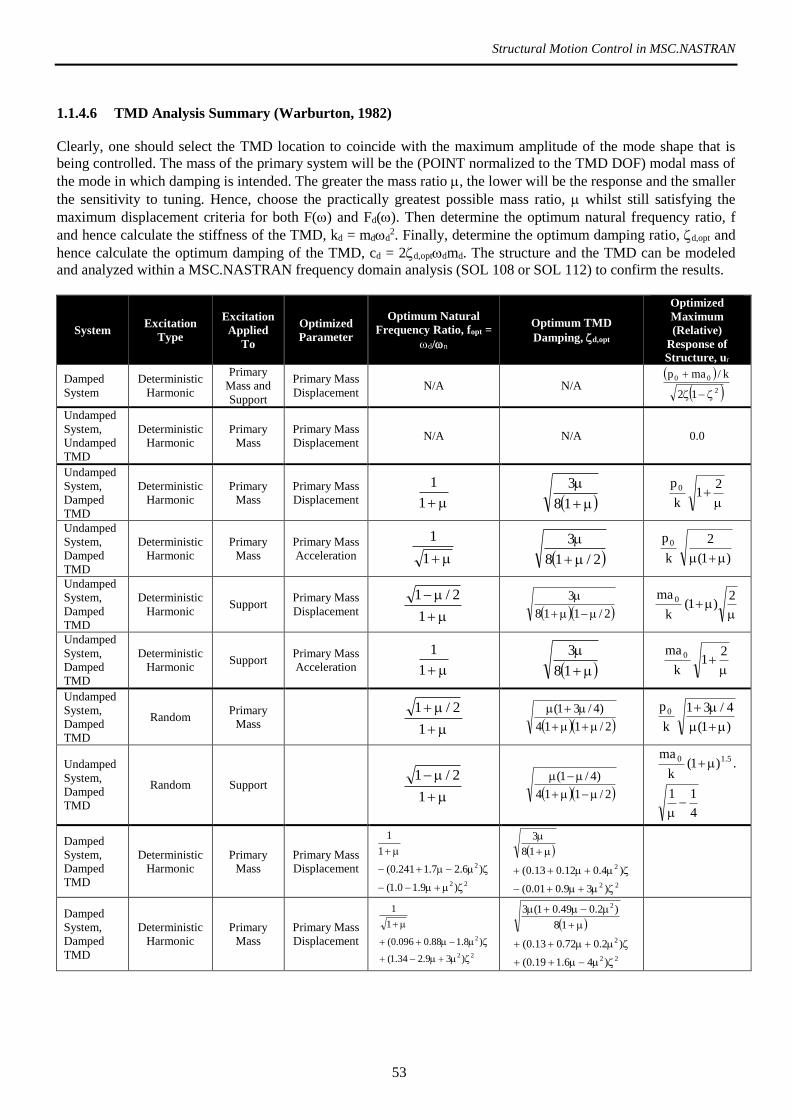
Structural Motion Control in MSC.NASTRAN
53
1.1.4.6 TMD Analysis Summary (Warburton, 1982)
Clearly, one should select the TMD location to coincide with the maximum amplitude of the mode shape that is
being controlled. The mass of the primary system will be the (POINT normalized to the TMD DOF) modal mass of
the mode in which damping is intended. The greater the mass ratio , the lower will be the response and the smaller
the sensitivity to tuning. Hence, choose the practically greatest possible mass ratio, whilst still satisfying the
maximum displacement criteria for both F() and Fd(). Then determine the optimum natural frequency ratio, f
and hence calculate the stiffness of the TMD, kd = mdd2. Finally, determine the optimum damping ratio, d,opt and
hence calculate the optimum damping of the TMD, cd = 2d,optdmd. The structure and the TMD can be modeled
and analyzed within a MSC.NASTRAN frequency domain analysis (SOL 108 or SOL 112) to confirm the results.
System Excitation
Type
Excitation
Applied
To
Optimized
Parameter
Optimum Natural
Frequency Ratio, fopt =
d/n
Optimum TMD
Damping, d,opt
Optimized
Maximum
(Relative)
Response of
Structure, ur
Damped
System
Deterministic
Harmonic
Primary
Mass and
Support
Primary Mass
Displacement N/A N/A
2
00
12
k/map
Undamped
System,
Undamped
TMD
Deterministic
Harmonic
Primary
Mass
Primary Mass
Displacement N/A N/A 0.0
Undamped
System,
Damped
TMD
Deterministic
Harmonic
Primary
Mass
Primary Mass
Displacement 1
1
18
3
21
k
p 0
Undamped
System,
Damped
TMD
Deterministic
Harmonic
Primary
Mass
Primary Mass
Acceleration 1
1
2/18
3
)1(
2
k
p 0
Undamped
System,
Damped
TMD
Deterministic
Harmonic Support
Primary Mass
Displacement
1
2/1
2/118
3
2
)1(k
ma 0
Undamped
System,
Damped
TMD
Deterministic
Harmonic Support
Primary Mass
Acceleration 1
1
18
3
21
k
ma 0
Undamped
System,
Damped
TMD
Random Primary
Mass
1
2/1
2/114
)4/31(
)1(
4/31
k
p0
Undamped
System,
Damped
TMD
Random Support
1
2/1
2/114
)4/1(
4
11
.)1(k
ma 5.10
Damped
System,
Damped
TMD
Deterministic
Harmonic
Primary
Mass
Primary Mass
Displacement
22
2
)9.10.1(
)6.27.1241.0(
1
1
22
2
)39.001.0(
)4.012.013.0(
18
3
Damped
System,
Damped
TMD
Deterministic
Harmonic
Primary
Mass
Primary Mass
Displacement 22
2
)39.234.1(
)8.188.0096.0(
1
1
22
2
2
)46.119.0(
)2.072.013.0(
18
)2.049.01(3

Structural Motion Control in MSC.NASTRAN
54
The displacement optimization parameter is used essentially to determine the safety and integrity of the structure
under external excitations. Since large accelerations of a structure under excitations produce detrimental effects on
functionality of nonstructural components, base shear and occupant comfort, minimizing structural accelerations
can also be a viable optimization criterion.
The effective damping often quoted for a system with a TMD is obtained simply by the following equation
eff = 1/(2Dopt())
as this is consistent with the definition of the maximum dynamic amplification for SDOF systems without TMD
which for small values of is
Dmax() = 1/(2)
For broadband seismic applications, Villaverde (1985) had suggested the following equations for optimum
parameters with mass ratio based on modal mass with eigenvector POINT normalized to location of TMD.
1fopt
opt,d
For broadband seismic applications, Fadek et. al. (1997) suggested the following equations for optimum parameters
with mass ratio based on modal mass with eigenvector POINT normalized to location of TMD.
11
1
1fopt
11opt,d
TMD are effective in seismic applications for structures with low damping, = 0.02. For structures with damping,
= 0.05, TMDs are not very effective since a very large mass ratio is required. TMDs are also not effective in
seismic applications of very stiff structures with periods 0.1-0.2s.

Structural Motion Control in MSC.NASTRAN
55
1.1.5 GL, ML Tuned Slosh Damper (TSD) Systems 1
TSDs can, in some cases, present a cost-effective alternative to Tuned Mass Dampers for reducing the response of
lively structures. Their principle strengths are low initial cost and virtually maintenance-free operation.
1.1.5.1 When To Employ TSDs
For a TSD to be the right solution, the following should be true: -
I. The problem motion of the structure is predominantly horizontal at the proposed location of the
damper.
II. The volume available for the damper is at least twice that of the TSD liquid which would provide the
required damper mass. This allows space for sloshing and the redundant mass of liquid.
III. The problem mode has a natural frequency below 2 Hz. Above this frequency, dampers become so
small that a prohibitively large number of damper tanks would be necessary to generate appreciable
damper mass.
The following is desirable: -
I. The natural frequency of the problem mode is accurately known (i.e. from testing). TSDs can be designed
to work across a range of natural frequency however, this can lead to increasing the complexity of the
design, having a variable damper mass or reducing the effectiveness of the damper for low amplitude
motions. The concession is dependent on the design route taken.
1.1.5.2 Operations of TSDs
Broadly speaking, two types of TSD have been fitted to structures: -
I. ‘Shallow tanks’ where the water height to length ratio is less than 0.1 and the damping is governed chiefly
by wave breaking and viscous action.
1 POWELL, Daniel. Tuned Slosh Dampers. Ove Arup & Partners Ltd., London, 2003.
0
500
1000
1500
2000
0 0.5 1 1.5 2
Nu
mb
er
of
Dam
pe
r T
an
ks
Design Frequency /Hz
Number of damper tanks required for a 1 tonne damper

Structural Motion Control in MSC.NASTRAN
56
II. ‘Deep tanks’ where the damping is generated by resistance elements in the centre of the tank applying drag
forces to the sloshing liquid
These two types of damper can be implemented in either rectangular or cylindrical tanks. If a structure is
susceptible to lateral excitation in two perpendicular directions, it is possible to use a rectangular damper with
matching sloshing frequencies in the relevant directions. More often than not, the liquid used in TSDs is water, the
main reason for this being cost.
1.1.5.2.1 Sloshing Frequency
The sloshing frequency of the nth mode of the tank geometry shown above is given by
a
hn
a
ngf n
tanh
2
1
Note that
I. The only modes of practical interest are the first two asymmetric modes i.e. n=1 the fundamental
sloshing frequency which is tuned to the structure and, to a lesser extent, n=3 (the mass of liquid
associated with this mode is much lower).
II. A tank of length ‘a’ has a maximum fundamental natural frequency given by a
g
2
1 i.e. this
frequency can’t be exceeded by raising h. In practice, for a given damper arrangement, the TSD
damping decreases with increasing h/a and it is unlikely you would choose to have this ratio
greater than 0.4. Note that h/a ratios of 0.1 to 0.35 are typical for a deep tank damper.
III. The sloshing frequency’s sensitivity to changes in ‘h’ is greatest when h is small hence, if a fixed-
length shallow tank damper is designed for a structure whose natural frequency is slightly different
from that predicted, the effective mass of the re-tuned damper can be very different from the design
value.
IV. This formula is developed using linear theory and the frequencies it predicts are for the related
sloshing modes i.e. for the fundamental mode the liquid surface is approximately a cosine between
0 and π. For shallow tanks, and deep tanks under large amplitude excitation, other sloshing modes
will become apparent.
Excitation
undisturbed liquid level
Damping
elements
(Deep Tank only)
h
a

Structural Motion Control in MSC.NASTRAN
57
1.1.5.2.2 Effective Mass and “Housner” Respresentation
Not all the liquid in a TSD takes part in the fundamental sloshing mode. There is a fraction, typically 20-30% in
deep tanks and <10% in shallow tanks, which can be considered as static mass added to the structure. The rest of
the liquid is actively sloshing and the mass of this liquid (the ‘effective mass’) can be thought of as that equivalent
to the mass in a TMD. An equivalent mechanical representation of liquid sloshing in tanks was developed by Housner in the 1950s and is illustrated below.
Housner representation of horizontally excited liquid in tank
where effective mass
a
h
h
a
M
M tanh
2527.01
(b is the damper tank’s internal breadth)
static mass 10 MMM
height of effective mass
a
h
a
h
a
h
h
h
sinh
2cosh
11
height of static mass
1
2
3
2
3tanh
4
8
10
h
a
h
ah
h
By evaluating the fundamental sloshing frequency from
a
hn
a
ngf n
tanh
2
1
the equivalent spring coefficient can be calculated for the Housner model using 12
1
M
kf
. The heights of the
effective and redundant mass give the dynamic moments about the base of the damper due to the ‘spring’ force and
h0
M.g
M0
M1
h1
h
a

Structural Motion Control in MSC.NASTRAN
58
inertia force, respectively. The values of these heights could be considered counter-intuitive, it is not unusual for
both values to be greater than h, particularly for shallower tanks. For deeper tanks h0 and h1 can be almost equal.
1.1.5.2.3 Sloshing Height
As part of the TSD design process it is necessary to estimate the sloshing height of the damper. Warnitchai and
Pinkaew’s (Engineering Structures Vol. 20 No. 7) method requires the iterative solving of an equation, Housner’s
method is more straight-forward but its form causes stability problems in an iterative spreadsheet, as is required for
evaluating the non-linear damping of a TSD. Another, simpler, method for estimating the sloshing height for deep
tank TSD is presented. The two basic assumptions are: -
I. The liquid surface is a half cosine wave.
II. The displacement of the centre of mass of the sloshing liquid is equal to the displacement of the
mass in an equivalent TMD.
Clearly this second assumption is a little simplistic as different regions of the TSD liquid move at different rates,
however, following these assumptions leads to the following expression: -
tmdda
h
2
2
where: - Λ is sloshing height above undisturbed liquid level
tmdd is displacement of an equivalent TMD
Better agreement between this formula and Housner’s method is achieved if a ‘fudge-factor’ of 0.75 is applied to
the above expression.
tmdda
h
275.0
2
To calculate the equivalent TMD performance, the damping of the TSD needs to be calculated (which in turn being
response dependent requires the sloshing height, hence the requirement for an iterative spreadsheet).
1.1.5.2.4 Stoke’s Number and Nonlinear Sloshing
Under modest levels of excitation, a TSD will slosh in the linear manner discussed previously with fundamental
natural frequency and effective mass close to values obtained from the formulae listed. At higher levels of
excitation sloshing non-linearities are present and new modes appear. There is also a new source of damping
through wave breaking. The transition from the linear state occurs at much lower levels of excitation in a shallow
tank damper. The parameter which governs the degree of non-linearity of sloshing of a TSD is the Stokes' Number,
Us.
3
24
h
aU s
At low values of Us (say <20), the TSD sloshing is close to linear. The principle deviation from linear behaviour, in
this Us range, being that the low-level and high-level sloshing heights are not of equal magnitude, the high-level is
around 30% greater at a Us of 10. Despite this, the formulae listed previously based on a linear model still hold. If
damping elements are not present to apply drag-forces on the fluid, damping is very low in this regime of Us
(typically <0.5%). As Us increases, the asymmetry about the undisturbed water height becomes more pronounced
and additional sloshing modes become apparent. Also, wave breaking becomes a significant source of damping. In
this non-linear sloshing regime, the importance of accurate tuning of the damper reduces and the eventually device
becomes more passive-energy-dissipater than tuned-vibration absorber.
1.1.5.2.5 Damping in TSDs
Damping is chiefly introduced by two different mechanisms in TSDs: -
I. Damping elements applying drag forces – obstructions fixed in the tank impede the sloshing of the liquid.

Structural Motion Control in MSC.NASTRAN
59
II. Wave breaking – at high Stokes' Numbers (i.e. in deep tank dampers under high amplitudes of excitation
and shallow tank dampers generally) significant wave breaking occurs which dissipates energy.
Damping Elements
Damping elements are obstructions immersed in the TSD liquid which the liquid flows past while sloshing. Drag
forces are applied by the damping elements on the liquid, this introduces damping into the system. Damping
elements are normally located in the centre of the tank where the peak velocity of the liquid is a maximum.
Typically damping elements obstruct around 25% of the flow area though this is dependent on the level of damping
required. Frequently used designs of damping element include baffles normal to the flow, perforated plates and
wire-mesh screens.
The drag forces objects immersed in fluids, can be thought of as being comprised of two parts: -
Skin-friction Dτ – the forces applied by shearing as the liquid passes the solid boundaries.
Pressure-drag DP – the net forces applied to the body due to differences in the upstream and downstream
pressure fields.
Broadly speaking, both components of the total drag force increase with fluid velocity V.
nVD where n is in the range 1.2 → 1.8
2P VD
The relative magnitude of these two drag components depends on the geometry of the object in the fluid. For
‘stream-lined’ bodies e.g. a flat plate parallel to the flow direction, the drag will be almost entirely skin friction
while for ‘bluff’ bodies e.g. a flat plate normal to the flow direction, the pressure drag will dominate. For some
cross-sections e.g. a cylinder, the ratio of these two drag forces varies considerably depending on the flow regime
and these simple relationships between drag and fluid velocity are of limited use.
The reason the composition of the drag forces on the damping elements is significant, is that this governs the
degree of non-linearity of the TSD damping. If the drag on the damping elements is mainly viscous and the value
of n in the expression above is close to 1 then the damping in the TSD is close to linear i.e. the damping ratio is
approximately constant. On the other hand, if the damping elements are such that the force on them is dominated
by the pressure-drag component e.g. baffles normal to the flow, the damping is non-linear and amplitude
dependent.
Realistically, damping elements which provide predominantly viscous drag across a wide range of Re e.g. baffles
parallel to the flow, are unlikely to provide sufficient total drag for the damping required in a TSD. One approach is
to use a very fine mesh of wires with cylindrical cross-section such that Re number remains low (say up to 2)
during sloshing. One practical concern with this design is that the mesh will clog up very easily, this would change
the blockage ratio and consequently the performance of the damper.
Warnitchai and Pinkaew developed an equation suggesting that for damping elements of constant CD, the damping
ratio of a TSD is directly proportional to the sloshing height, Λ. This linear relationship is verified by experiment
however, the quantitative predictions from the equation are poor if realistic values for CD are substituted into the
expression, the damping levels predicted being far too low.
Flat plates normal to flow have a drag coefficient which is approximately constant across a wide range of Re. This
is because of the small proportion of surface area in the flow-wise direction for the liquid to shear against, also the
point at which fluid passing the plate separates from the surface (i.e. the edges of the plate) is independent of Re,
meaning the wake area (area over which pressure-drag acts) at the rear of the plate will remain constant. Hence the
drag is dominated by the pressure-drag and increases with V2. Therefore, if baffles normal to the sloshing direction
are used as damping elements, the TSD damping is approximately proportional to sloshing height. Thus, this type
of damping element produces very low damping levels at very low amplitudes of excitation.
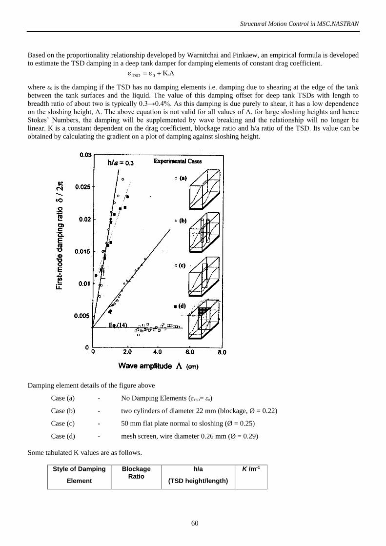
Structural Motion Control in MSC.NASTRAN
60
Based on the proportionality relationship developed by Warnitchai and Pinkaew, an empirical formula is developed
to estimate the TSD damping in a deep tank damper for damping elements of constant drag coefficient.
.K0TSD
where ε0 is the damping if the TSD has no damping elements i.e. damping due to shearing at the edge of the tank
between the tank surfaces and the liquid. The value of this damping offset for deep tank TSDs with length to
breadth ratio of about two is typically 0.3→0.4%. As this damping is due purely to shear, it has a low dependence
on the sloshing height, Λ. The above equation is not valid for all values of Λ, for large sloshing heights and hence
Stokes’ Numbers, the damping will be supplemented by wave breaking and the relationship will no longer be
linear. K is a constant dependent on the drag coefficient, blockage ratio and h/a ratio of the TSD. Its value can be
obtained by calculating the gradient on a plot of damping against sloshing height.
Damping element details of the figure above
Case (a) - No Damping Elements (εTSD= ε0)
Case (b) - two cylinders of diameter 22 mm (blockage, Ø = 0.22)
Case (c) - 50 mm flat plate normal to sloshing (Ø = 0.25)
Case (d) - mesh screen, wire diameter 0.26 mm (Ø = 0.29)
Some tabulated K values are as follows.
Style of Damping
Element
Blockage Ratio
h/a
(TSD height/length)
K /m-1

Structural Motion Control in MSC.NASTRAN
61
vertical cylinders 0.22 0.3 0.33
Baffles normal
to flow
0.25 0.3 1.80
“ 0.17 0.4 1.31
“ 0.25 0.4 1.65
“ 0.33 0.4 2.39
For three cases, the trend is for a straight line crossing the y-axis at ε0 (~0.003 in this case) the exception is case (d).
For this case the y-axis is intersected at a significantly higher value and there is a less obvious linear fit to the data.
One might expect cases (b) and (d) to exhibit similar trends, both damping elements consisting essentially of flow
obstructions of circular cross-section. The difference lies in the Re numbers. The Re number of the flow past
damping elements varies between zero, when the liquid is instantaneously stationary at the extremity of sloshing,
and some maximum value, a quarter of a sloshing cycle later, when the liquid surface is nominally flat and the
velocity across the damping elements a maximum. The characteristic dimensions for the calculation of Re number
in cases (b) and (d) are 22 and 0.26 mm, respectively. Consequently, for a sloshing height of 2 cm, the
corresponding theoretical maximum Re numbers are 350 and 4. Inspection of the CD versus Re figure indicates that
the drag coefficients in the two TSDs vary across very different ranges, hence drag forces and consequently
damping characteristics are very different.
In order to calculate Re numbers in a TSD, an estimate of the liquid speed at the centre of the tank is required. A
velocity potential function for the liquid is derived in Warnitchai and Pinkaew based on linear theory and, hence,
only applicable to deep tank dampers. By differentiating this expression with respect to the spatial coordinate in the
sloshing direction (x), an expression for the liquid velocity is obtained, dependent on time and position in the tank.
Substituting in the x value for the mid-point of the tank yields: -
)2sin(.
sinh
)(cosh
. 1tf
a
h
a
hz
U x
where the previously defined symbols have the same meanings and: -
xU is the liquid velocity in the horizontal sloshing direction / m/s
z is the vertical co-ordinate with origin at the undisturbed liquid surface / m
1f is the fundamental sloshing mode of the TSD / Hz
t is time / s
For a given , h and a, the magnitude of xU will be a maximum when )2sin( 1tf =1. If this is substituted into the
above equation, the result is a profile of xU magnitudes against z which can be integrated up to obtain a mean
value of xU , xU where: -
h
aU x
This is the magnitude of a sinusoid so a more representative value is the RMS of this i.e.: -
2h
aU
RMSx
This equation can be used to generate the velocity term when calculating practical values of Re number for the flow
across damping elements. Establishing the Re number for damping elements of circular section helps give a

Structural Motion Control in MSC.NASTRAN
62
qualitative prediction of their behaviour. If the Re number is very low e.g. < 2, the drag will have a significant
viscous component and the TSD will have useful damping at very low levels of excitation (e.g. 2 cm sloshing
height for a typical deep tank TSD) and the TSD’s damping will have less dependence on sloshing height. If
however the Re number is larger than 100, the drag will be dominated by the pressure-drag and, for all practical Re
numbers, the drag coefficient will be approximately constant (assuming the Re Number isn’t going to exceed 105 !),
consequently, the TSD damping will be approximately proportional to sloshing height. As all TSDs with practical
damping levels exhibit some dependence on response, the damping ratio will fall-off either side of resonance as the
magnification factor reduces.
Wave Breaking
At higher Stokes’ Numbers (i.e. high amplitudes of excitation), surface tension is no longer strong enough to keep
the liquid surface continuous and ‘wave breaking’ occurs. There are significant losses associated with this process
which introduce additional damping into the system. In this sloshing regime, the TSDs behaviour deviates
significantly from the linear models used to represent lower amplitude excitation and it is no longer valid to use
them. In our existing TSD literature, there is no method presented for predicting the damping due to wave breaking
and. Typically dampers of 1 to 1.5% of the modal mass of a lightly damped structure can increase the effective
structural damping to between 4 and 5%. One of the main advantages of TSDs which rely on wave breaking to
provide the damping is that the performance of the damper is relatively insensitive to tuning ratio.
1.1.5.2.6 Conditions at Resonance
As for all resonant systems with damping, TSDs exhibit a frequency shift such that the maximum magnification
factor (and hence maximum sloshing height in a ‘frequency-sweep’ test) occurs at tuning-ratios of less than 1,
where tuning ratio is defined as: -
1f
fr e
where ef is excitation frequency /Hz and
1f is the fundamental sloshing frequency
The tuning ratio where the resonance occurs in conventional TMDs is given by: -
221 r
where ε is the damping ratio.
For the case of deep tank TSDs with damping elements, an additional frequency shift occurs. This can be
qualitatively explains as follows: - the liquid flow past the damping elements is unsteady and continuously
accelerating and decelerating. To drive these changes in velocity (by Newton’s Second Law) a variable pressure
gradient must exist in the liquid. As the damping elements are immersed in the liquid, they experience a force due
to this pressure gradient (as described in ‘Morison’s Equation’) and consequently react a drag force back onto the
liquid. This drag-force is conservative (as it is transferring momentum elastically between TSD liquid and
structure) and introduces no damping yet, as it is applying a force on the liquid, it is responsible for a reduction in
natural frequency. The frequency shift due to this effect is calculated analytically in Warnitchai and Pinkaew.
However, in tests this theoretical treatment was found to over-predict the magnitude of the frequency reduction.
From the tests carried out on the Arup Gatwick project, 2% was found to be a practical reduction in the TSD
fundamental frequency. This factor allows for both the reduction due to damping and blockage. This figure was
seen to be approximately correct for damping ratios of order 5-10% and blockage ratios from 0.15-0.35. The
frequency at which the maximum lateral force exerted by the tank on the structure occurs does not necessarily
correspond with the frequency of maximum sloshing height. Indeed, dependent on the size of the redundant liquid
mass and the mass of the empty tank, the frequency of maximum lateral force can be higher or lower than 1f .

Structural Motion Control in MSC.NASTRAN
63
1.1.5.3 Deep or Shallow Tank?
As previously discussed, TSDs can be thought of as being shallow tank (h/a<≈0.1) or deep tank.
1.1.5.3.1 Deep Tank
Performance can be predicted analytically – as have been discussed, analytical methods exist for predicting the
behaviour of deep tank dampers. Given the cost of testing TSDs, this is a considerable asset. High mass – although
the proportion of liquid which contributes to the sloshing (effective mass) increases as a damper is made shallower,
the absolute effective mass decreases. Thus, achieving the same mass ratio between structure and damper with
shallow tanks requires more tanks and, in all likelihood, more complexity, as dampers might need to be stacked.
1.1.5.3.2 Shallow Tank
Relatively insensitive to tuning ratio – as the sloshing of a shallow tank damper is non-linear, the Housner
representation is not a good representation of the behaviour. Shallow tank dampers act more as passive energy
absorbers than TMDs or deep tank TSDs, consequently they reduce the worst-case response to a lesser extent than
a well-tuned TMD but they achieve a useful reduction across a broad range of tuning ratios.
1.1.5.3.3 Practical Considerations
Due to the relatively low mass of a shallow tank damper, many tanks are usually required to achieve the required
damper to structure ratio. Hence this style of TSD lends itself to prefabricated stacks of dampers which can be fixed
to a supporting frame on the structure (see reference 1 for examples of this). Once fabricated the only option
available for tuning the frequency of the dampers is adjusting the water depth. Thus, if the natural frequency of the
structure is not known accurately prior to design (i.e. has not been measured), the effective mass and mass ratio of
the dampers can vary significantly.
For the case of deep tank TSDs, it is more probable that the damper mass will be provided by a small number of
large tanks. It is therefore likely that it will be practical to install an adjustable baffle within each of the tanks
allowing variation of the damper dimension in the sloshing direction. This allows greater control of the effective
mass of the TSDs across a range of frequencies, as when a reduction in TSD design frequency is required, the
reduction in depth can be accompanied/replaced by an increase in length (the converse is also true but it is unlikely
that the damper being too massive would be a problem).
In summary, a shallow tank TSD has desirable characteristics if the in-service frequency of the structure is likely to
vary (say +/- 5%) about some well-defined initial value, while a deep tank TSD might be the preferred option if the
frequency is not likely to vary significantly in service (though this might be allowed for by ‘spread-tuning’). If the
design of the TSD is developing in tandem with the structure, deep tank TSDs are probably the more sensible
option as it’s more likely their design-frequency can be changed without compromising their performance.
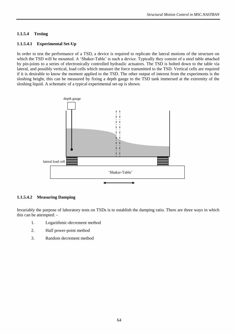
Structural Motion Control in MSC.NASTRAN
64
1.1.5.4 Testing
1.1.5.4.1 Experimental Set-Up
In order to test the performance of a TSD, a device is required to replicate the lateral motions of the structure on
which the TSD will be mounted. A ‘Shaker-Table’ is such a device. Typically they consist of a steel table attached
by pin-joints to a series of electronically controlled hydraulic actuators. The TSD is bolted down to the table via
lateral, and possibly vertical, load cells which measure the force transmitted to the TSD. Vertical cells are required
if it is desirable to know the moment applied to the TSD. The other output of interest from the experiments is the
sloshing height, this can be measured by fixing a depth gauge to the TSD tank immersed at the extremity of the
sloshing liquid. A schematic of a typical experimental set-up is shown.
1.1.5.4.2 Measuring Damping
Invariably the purpose of laboratory tests on TSDs is to establish the damping ratio. There are three ways in which
this can be attempted: -
1. Logarithmic-decrement method
2. Half power-point method
3. Random decrement method
lateral load cell
depth gauge
‘Shaker-Table’

Structural Motion Control in MSC.NASTRAN
65
1.1.5.5 Miscellaneous Design Information
1.1.5.5.1 Separator-Plates
It will often be the case that several damper tanks are required to achieve the required damper mass. In this case it
might prove economic to manufacture one large tank then segment this longitudinally and transversely with
separator plates.
Longitudinal Separator-Plates
In the longitudinal (slosh-wise) direction the plates are installed to prevent excessively large transverse waves due
to reflections. The rule of thumb used is to limit the breadth of each individual slosh tank to half its length. As
the longitudinal plates will have little or no dynamic head difference across them, the seal surrounding the separator
plate is of little importance. Neither, for the same reason, is there a requirement for them to be particularly stiff.
Transverse Separator-Plates
In contrast, the transverse separator plates have a significant dynamic force across them when the TSD is excited as
shown in figure below. For a given water height, translating the plate back and for changes the sloshing frequency
of a TSD so transverse plates will also be required when TSDs are being designed for structures whose natural
frequency is not accurately known.
If there is excessive flexure of the plates during operation then the normal mode of the TSD will be modified
slightly and, experiments indicate that, the natural frequency will be reduced. The seal surrounding transverse
separator plates has a significant impact on the performance of the damper.
At the sloshing extremity shown above, TSD liquid will seep from damper 1 to damper 2 at a maximum rate. Half a
cycle later, water will seep in the opposite direction at a maximum rate. The continuous passage of the liquid back-
and-for under the separator-plate introduces damping into the TSD. The characteristics of the damping introduced
are dependent on the size of the gap surrounding the separator-plate. As the gap is reduced, the ‘magnitude’ of the
damping will reduce yet the viscous element of damping will increase (due to the fall in the Re number).
The effect of the gaps was to introduce a considerable amount of damping at low-excitation levels, in effect
‘linearising’ the damper to some degree. Damping levels at higher excitation levels were found to be closer to
predictions, the reason being that the proportion of the damping due to seepage was small compared to the liquid
passing the Damping Elements at a higher rate.
1.1.5.5.2 Additional Considerations
Add anti-freeze if a TSD is to be used externally. Stagnant pools need to be treated for algae and legionaires’
disease. Seal the tank, evaporation will change the TSDs slosh frequency and affect the performance
Seepage under
separator-plate
head difference
1 2

Structural Motion Control in MSC.NASTRAN
66
1.1.5.6 Design Procedure for Deep Tank TSDs
The following is a suggested possible design process for deep tank TSDs: -
1. Establish the level of damping required for desired structural response and convert this to an equivalent
peak DAF ( = ½ε).
2. Select a suitable damper to structure modal mass ratio, μ. e.g. using figure below. NB. The DAFs in the
figure are for optimum damping and are unlikely to be achievable in practice.
3. Calculate the optimum TSD sloshing frequency using structureopt ff
1
1.
4. Choose TSD dimensions such that optff 02.11 using the sloshing frequency formula (The factor of
1.02 accounts for the likely frequency shift due to damping and blockage in the TSD).
5. Calculate M1 (the active sloshing mass of the TSDs) based on the chosen TSD dimensions (assume a
breadth of half the length).
6. Calculate the number of dampers required to provide the required mass ratio using 1
mod
MM
N al .
Do the dampers fit in the space available?
7. Select a ‘K’ (damping per sloshing height) value from table of values presented before and assume
εo=0.03.
8. Plot the DAF for the system in a spreadsheet.
9. If the DAF is below the desired level across the required frequency range, start a sensitivity study (try
varying f1 , M1 and K). If not, inspect a plot of the damping against frequency, try changing K (within
reason) so that the damping is closer to optimum in the region of interest. If this doesn’t work, try a higher mass ratio.
Mass ratio (Mdamper /Mstructure )
Max DAF at
opt. damping
structural damping

Structural Motion Control in MSC.NASTRAN
67
1.2 GL, ML Active Structural Motion Control – Control System Analysis
A control system provides feedback (output) to an input. This is useful to model an Active Mass Damper (AMD).
The modelling of a control system involves the definition of an input-output relationship, i.e. a transfer function.
This can be defined using the TF bulk data entry. Nonlinearities can be simulated via the NOLINi entries with
which nonlinear transient loads are expressed as functions of displacements or velocities. Complex eigenvalue
analysis can be used to determine stability when control systems include damping and unsymmetrical matrices.

Structural Motion Control in MSC.NASTRAN
68
BIBLIOGRAPHY
1. CONNOR, Jerome. Introduction to Structural Motion Control. Prentice Hall, Massachusetts Institute of
Technology, 2003.
2. POWELL, Daniel. Tuned Slosh Dampers. Arup Research and Development, Ove Arup & Partners Ltd.,
London, 2003.
3. BACHMANN, Hugo. Vibration Problems in Structures Practical Guidelines. Birkhauser, Berlin, 1995.
4. EWINS, D.J. Modal Testing Theory, Practice and Application Second Edition. Research Studies Press Ltd,
England, 2000.
5. JIMIN, He and ZHI-FANG, Fu. Modal Analysis. Butterworth-Heinemann, Great Britain, 2001.
6. BRUEL & KJAER. Vibration Analysis, Measurement and Testing. Denmark, 2001.
7. CLOUGH R.W. & PENZIEN J. Dynamics of Structures 2nd Edition. McGraw-Hill Book Co., United States,
1993.
8. SMITH, J.W. Vibration of Structures, Application in Civil Engineering Design. Chapman and Hall, London,
1988.
9. BEARDS, C. F. Structural Vibration Analysis, Modelling, Analysis and Damping in Vibrating Structures.
Ellis Horwood, London, 1983.
10. SELVAM, Dr. R.P & GOVINDASWAMY, Suresh. Aeroelastic Analysis of Bridge Girder Section Using
Computer Modelling. University of Arkansas, May 2001.
11. SIMIU and SCALAN. Wind Effects on Structures, An Introduction to Wind Engineering.