Embed Size (px)
Citation preview
Structural Optimization of a Planar Reciprocal Framewith Triangular Topology
by
Gerry H.F. Ip
B.A.Sc., Department of Civil EngineeringUniversity of Toronto (2015)
MASSACHSET LNSTTTOF TECHNOLOGY
JUN 0 7 2016
LIBRARIES
ARCHIVESSUBMITTED TO THE DEPARTMENT OF CIVIL AND ENVIRONMENTAL
ENGINEERING IN PARTIAL FULFILLMENT OF THE REQUIREMENTS FOR THEDEGREE OF
MASTER OF ENGINEERING IN CIVIL AND ENVIRONMENTAL ENGINEERINGAT THE
MASSACHUSETTS INSTITUTE OF TECHNOLOGY
JUNE 2016
2016 Gerry H.F. Ip. All rights reserved.
The author hereby grants to MIT permission to reproduce and to distribute publicly paper andelectronic copies of this thesis document in whole or in part in any medium now known or
hereafter created.
Signature redactedSignature of Author:
Department of Civil
Certified by:
Lecturer of Civil
Certified by:
Professor of Civil
Accepted by:
Donald and Martha Harleman Professor of CivilChair, Departmental C
and Environmental 9ngiheeringMay 10, 2016
Signature redactedCorentin Fivet
and Environmna ngineeringTjois Supevi YZ
Signature redacted/7 John A. Ochsei(rf
and Ep4ironmental EngineeringThesis Supervisor
Signature redactedI I~Ifeidi Kepf 7
and Environmental Engineeringommittee for Graduate Students

Structural Optimization of a Planar Reciprocal Framewith Triangular Topology
by
Gerry H.F. Ip
Submitted to the Department of Civil and Environmental Engineering on May 10, 2016 in PartialFulfillment of the Requirements for the Degree of Master of Engineering in Civil and
Environmental Engineering
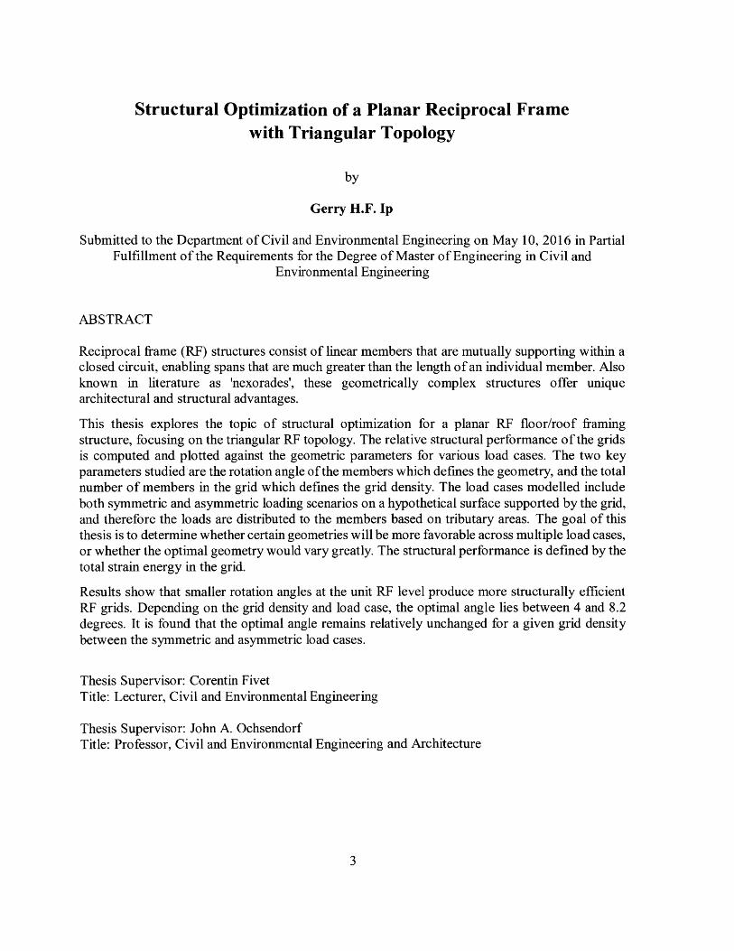
ABSTRACT
Reciprocal frame (RF) structures consist of linear members that are mutually supporting within aclosed circuit, enabling spans that are much greater than the length of an individual member. Alsoknown in literature as 'nexorades', these geometrically complex structures offer uniquearchitectural and structural advantages.
This thesis explores the topic of structural optimization for a planar RF floor/roof framingstructure, focusing on the triangular RF topology. The relative structural performance of the gridsis computed and plotted against the geometric parameters for various load cases. The two keyparameters studied are the rotation angle of the members which defines the geometry, and the totalnumber of members in the grid which defines the grid density. The load cases modelled includeboth symmetric and asymmetric loading scenarios on a hypothetical surface supported by the grid,and therefore the loads are distributed to the members based on tributary areas. The goal of thisthesis is to determine whether certain geometries will be more favorable across multiple load cases,or whether the optimal geometry would vary greatly. The structural performance is defined by thetotal strain energy in the grid.
Results show that smaller rotation angles at the unit RF level produce more structurally efficientRF grids. Depending on the grid density and load case, the optimal angle lies between 4 and 8.2degrees. It is found that the optimal angle remains relatively unchanged for a given grid density
between the symmetric and asymmetric load cases.
Thesis Supervisor: Corentin FivetTitle: Lecturer, Civil and Environmental Engineering
Thesis Supervisor: John A. OchsendorfTitle: Professor, Civil and Environmental Engineering and Architecture
3


Acknowledgements
I would like to thank Dr. Corentin Fivet for taking the time to understand my research interestsand introducing me to the intriguing subject of reciprocal frame structures. Dr. Fivet has been ofimmense support throughout my year at MIT, both as my thesis advisor and as my go-to advisorfor any structural engineering inquiries I have from other coursework. I am grateful for hisgenerosity in always being available for us.
I would also like to thank Professor John Ochsendorf for providing constructive feedback on thisthesis, and for his patience and kindness throughout the year. Professor Ochsendorf has alwaysbeen on the lookout to bring the next leading structural engineer to MIT for our class to learn from,and the experience has been rewarding.
Thank you to my great classmates: I couldn't have asked for a better group of friends to spend thedays and nights with in the MEng room.
Finally, thank you to my family for their love and support throughout my academic endeavors, andto my friends in Canada for their continued moral support.
5

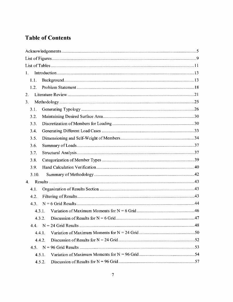
Table of Contents
Acknow ledgem ents.....................................................................................................................5
List of Figures............................................................................................................................9
List of Tables ............................................................................................................................ 11
1. Introduction.......................................................................................................................13
1.1. Background.................................................................................................................13
1.2. Problem Statement ...................................................................................................... 18
2. Literature Review .............................................................................................................. 21
3. M ethodology ..................................................................................................................... 25
3.1. Generating Typology ............................................................................................... 26
3.2. M aintaining Desired Surface Area.......................................................................... 30
3.3. D iscretization of M embers for Loading .................................................................. 30
3.4. Generating D ifferent Load Cases ............................................................................ 33
3.5. Dim ensioning and Self-W eight of M embers............................................................ 34
3.6. Sum m ary of Loads......................................................................................................37
3.7. Structural Analysis......................................................................................................37
3.8. Categorization of M ember Types ............................................................................ 39
3.9. Hand Calculation Verification................................................................................. 40
3.10. Sum m ary of M ethodology ................................................................................... 42
4 . R esu lts .............................................................................................................................. 4 3
4.1. Organization of Results Section .............................................................................. 43
4.2. Filtering of Results......................................................................................................43
4.3. N = 6 Grid Results ...................................................................................................... 44
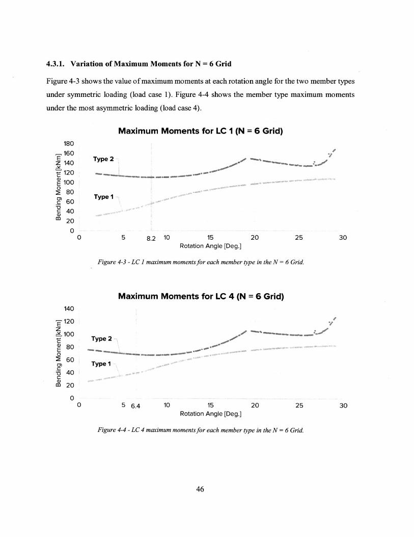
4.3.1. V ariation of M aximum M oments for N = 6 Grid .................................................. 46
4.3.2. D iscussion of Results for N = 6 Grid................................................................ 47
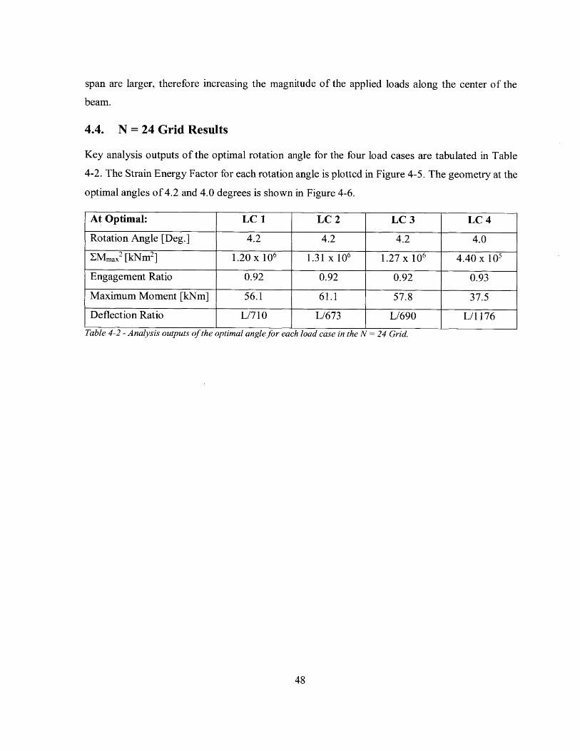
4.4. N = 24 Grid Results ............................................................................................... 48
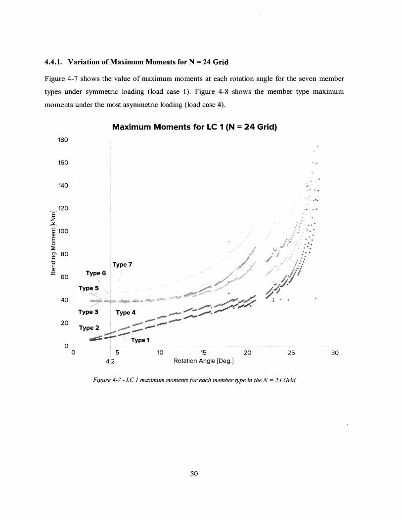
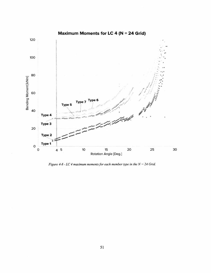
4.4.1. V ariation of M aximum M om ents for N = 24 Grid ................................................ 50
4.4.2. D iscussion of Results for N = 24 Grid.............................................................. 52
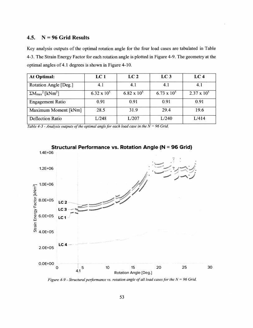
4.5. N = 96 Grid Results .................................................................................................... 53
4.5.1. V ariation of M aximum M oments for N = 96 Grid ................................................ 54
4.5.2. D iscussion of Results for N = 96 Grid..................................................................57
7
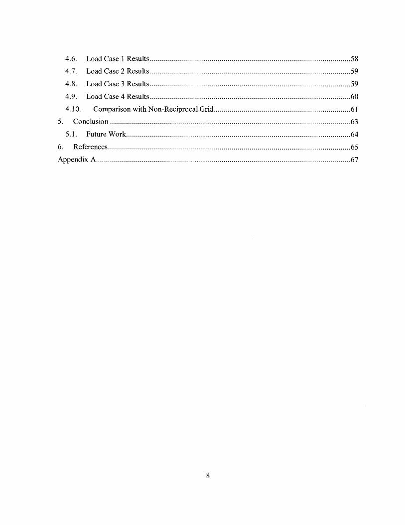
4.6. Load Case I Results .................................................................................................... 58
4.7. Load Case 2 Results .................................................................................................... 59
4.8. Load Case 3 Results .................................................................................................... 59
4.9. Load Case 4 Results .................................................................................................... 60
4.10. Comparison with Non-Reciprocal Grid .................................................................... 61
5 . C o n clu sio n ........................................................................................................................ 6 3
5. 1. Future W ork ................................................................................................................ 64
6 . R eferences ......................................................................................................................... 6 5
A p p en d ix A ............................................................................................................................... 6 7
8
List of Figures
Figure 1-1 - Honnecourt's planar grillage assembly (sketched by A.E. Plroozfar) (Larsen 2008)..
................................................................................................................................................. 1 3Figure 1-2 - Regular unit RFs (a); Irregular unit RFs (b) (Kohlhammer and Kotnik 2011). ....... 14Figure 1-3 - Regular RF grids (a); Irregular RF grids (b) (Kohlhammer and Kotnik 2011).........14Figure 1-4 - Example of a complex RF (Larsen 2008). .......................................................... 14Figure 1-5 - Interior of the Seiwa exhibition hall (Larsen 2008).............................................15
Figure 1-6 - Section drawing of the Seiwa exhibition hall (drawn by Tadashi Hamauzu) (Larsen
2 0 0 8 ).........................................................................................................................................1 5Figure 1-7 - Kreod Pavilion (K ingsford)................................................................................ 17Figure 1-8 - An "arch" type deployable emergency RF structure (Larsen and Lee 2013)......17
Figure 1-9 - A "planar" type emergency RF structure (Larsen and Lee 2013). ....................... 17
Figure 1-10 - A "hanging" type emergency RF structure (Larsen and Lee 2013).....................17
Figure 1-11 - N = 24 grids with varying rotation angles.............................................................19
Figure 1-12 - Schematic of applied loads, as shown on the N = 24 Grid. ............................... 19
Figure 2-1 - Example of an RF grid with rectangular topology studied by Gelez et al (2011).....21
Figure 2-2 - Comparison between an RF grid and a regular grid for an irregular perimeter (Gelez,A ubry, and V audeville 2011). ................................................................................................... 21Figure 2-3 - Planar RF grid configurations studied by Parigi and Kirkegaard (2013). ............ 22Figure 3-1 - Sequence of methodology used to generate parameterized model.......................25
Figure 3-2 - G enerating the unit RF...................................................................................... 26
Figure 3-3 - Diagrammatic procedure of generating the N = 6 Grid. ...................................... 27
Figure 3-4 - Diagrammatic procedure of generating the N = 24 Grid. .................................... 27
Figure 3-5 - Support conditions of members in an RF grid. .................................................. 28
Figure 3-6 - Plan view ofN = 6 grid showing the support conditions for each member.......28
Figure 3-7 - Examples of the N = 24 grid at various rotation angles.......................................29
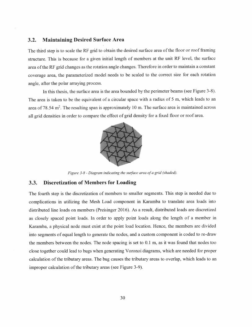
Figure 3-8 - Diagram indicating the surface area of a grid (shaded). .......................................... 30
Figure 3-9 - Example of the Voronoi bug. ............................................................................. 31Figure 3-10 - Example showing the removal of nodes in certain cases...................................32
Figure 3-11 - T ributary areas.....................................................................................................32
Figure 3-12 - D iscretized distributed loads. ........................................................................... 33
Figure 3-13 - Trimmed Voronoi diagram for distributing the concentrated load in Load Case 3.34
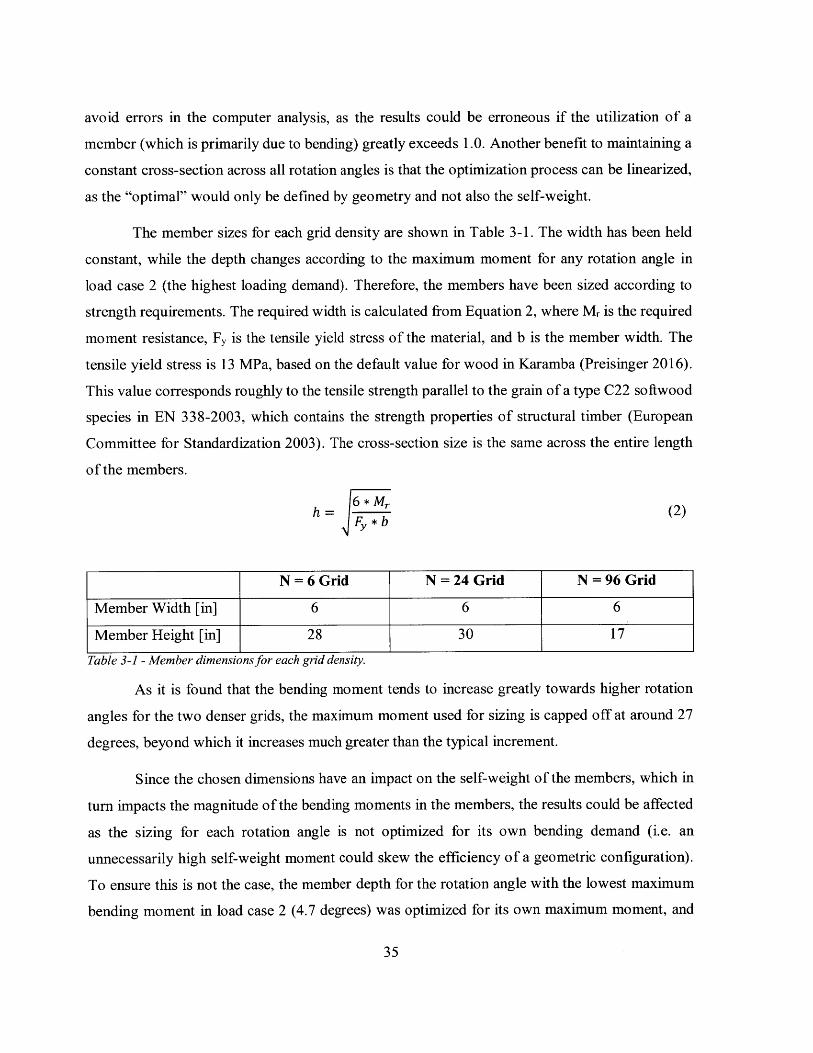
Figure 3-14 - Trimmed Voronoi diagram for Load Case 4. .................................................... 34
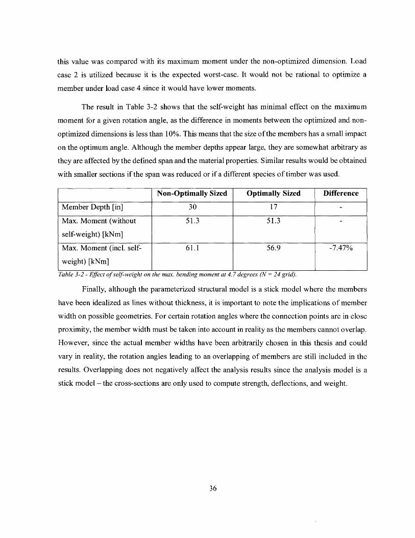
Figure 3-15 - Uniform line loads for self-weight. ...................................................................... 34
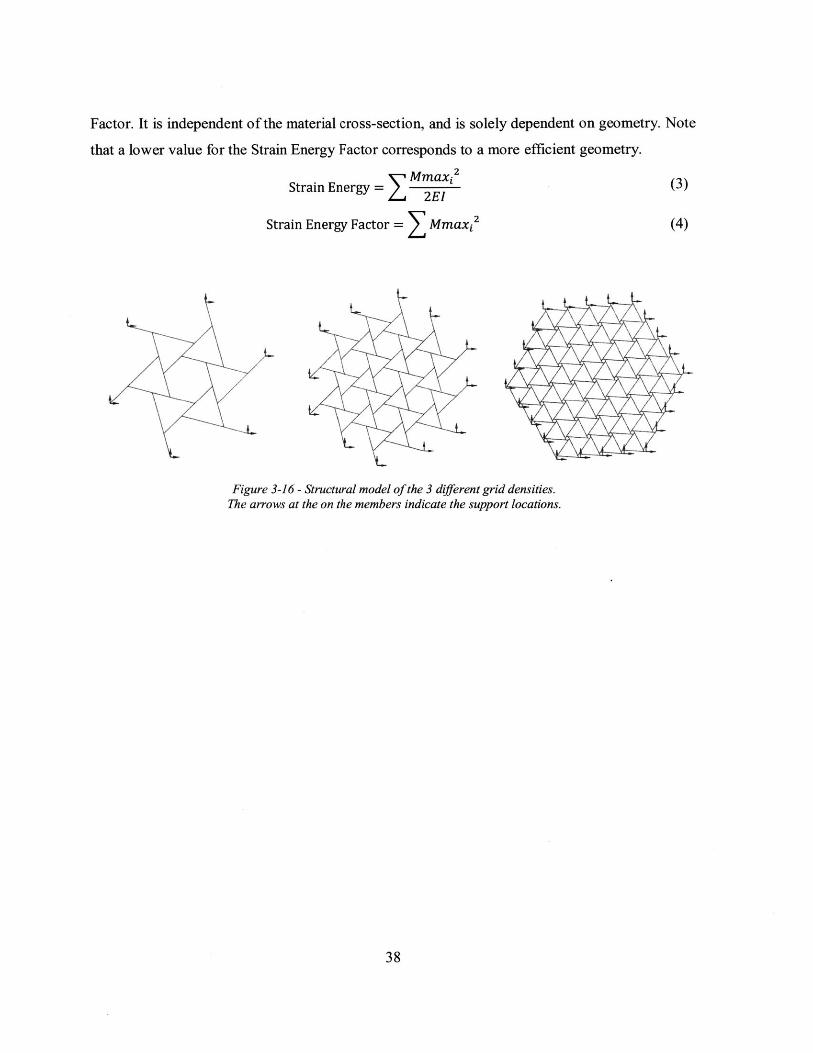
Figure 3-16 - Structural model of the 3 different grid densities. ............................................ 38
Figure 3-17 - M ember types in an N = 6 Grid........................................................................ 39Figure 3-18 - M ember types in an N = 24 Grid...................................................................... 39
Figure 3-19 - Unknown forces on the two member types.......................................................41
Figure 4-1 - Structural performance vs. rotation angle of all load cases for the N = 6 Grid.........45
Figure 4-2 - Optimal geometries for the N = 6 Grid................................................................45
Figure 4-3 - LC 1 maximum moments for each member type in the N = 6 Grid............46
9
Figure 4-4 - LC 4 maximum moments for each member type in the N = 6 Grid. .................... 46
Figure 4-5 - Structural performance vs. rotation angle of all load cases for the N = 24 Grid.......49
Figure 4-6 - Optimal geometries for the N = 24 Grid............................................................. 49Figure 4-7 - LC 1 maximum moments for each member type in the N = 24 Grid. .................. 50
Figure 4-8 - LC 4 maximum moments for each member type in the N = 24 Grid...................51
Figure 4-9 - Structural performance vs. rotation angle of all load cases for the N = 96 Grid.......53
Figure 4-10 - Optimal geometry for the N = 96 Grid. ............................................................ 54Figure 4-11 - LC 1 maximum moments for each member type in the N = 96 Grid.................55Figure 4-12 - LC 4 maximum moments for each member type in the N = 96 Grid. ................ 56Figure 4-13 - Example of a non-reciprocal grid with geometry similar to an RF grid. ............ 61
Figure 4-14 - RF Grid at a rotation angle of 18.6 degrees. .................................................... 61
Figure 5-1 - Optimal geometries for load case 1. .................................................................. 64
10
List of Tables
Table 1-1 - Sum m ary of load cases......................................................................................... 19Table 3-1 - M ember dimensions for each grid density. .......................................................... 35Table 3-2 - Effect of self-weight on the max. bending moment at 4.7 degrees (N = 24 grid). ..... 36Table 3-3 - M agnitude of live loads for all grid densities. ...................................................... 37Table 3-4 - Magnitude of dead loads for each grid density....................................................37Table 3-5 - Comparison of hand calculation with Karamba output.........................................41Table 4-1 - Analysis outputs of the optimal angle for each load case in the N = 6 Grid. ......... 44Table 4-2 - Analysis outputs of the optimal angle for each load case in the N = 24 Grid. ........... 48Table 4-3 - Analysis outputs of the optimal angle for each load case in the N = 96 Grid. ........... 53Table 4-4 - Analysis outputs from the optimal geometry for Load Case 1..............................58Table 4-5 - Analysis outputs from the optimal geometry for Load Case 2..............................59
Table 4-6 - Analysis outputs from the optimal geometry for Load Case 3...............................59Table 4-7 - Analysis outputs from the optimal geometry for Load Case 4..............................60Table 4-8 - Comparison of analysis outputs between an RF Grid and Non-RF Grid...............61
11

12
1. Introduction
Reciprocal frame (RF) structures consist of linear members that support one another within a
closed circuit, hence the origin of the term "reciprocal". This mutually supporting nature of the
structure enables spans that are much greater than the length of an individual member. RF
structures have also been referred to in literature as 'nexorades', where each member is termed a
'nexor', meaning 'link' in Latin (Baverel 2004).
1.1. Background
As Larsen (2008) suggests in her work "Reciprocal Frame Architecture", it is difficult to pinpoint
exactly when the first RF structure was built. Evidence of historic structures that bear similarity to
RF principles can be found in both Japanese and Western architecture, dating as early as the 1 2 th
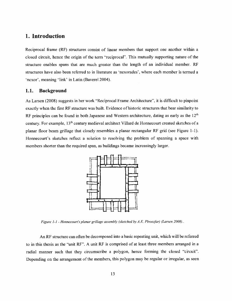
century. For example, 1 3 th century medieval architect Villard de Honnecourt created sketches of a
planar floor beam grillage that closely resembles a planar rectangular RF grid (see Figure 1-1).
Honnecourt's sketches reflect a solution to resolving the problem of spanning a space with
members shorter than the required span, as buildings became increasingly larger.
t~2~ . 9 I ~ fl
Figure 1-1 - Honnecourt's planar grillage assembly (sketched by A.E. Plroozfar) (Larsen 2008)..
An RF structure can often be decomposed into a basic repeating unit, which will be referred
to in this thesis as the "unit RF". A unit RF is comprised of at least three members arranged in a
radial manner such that they circumscribe a polygon, hence forming the closed "circuit".
Depending on the arrangement of the members, this polygon may be regular or irregular, as seen
13
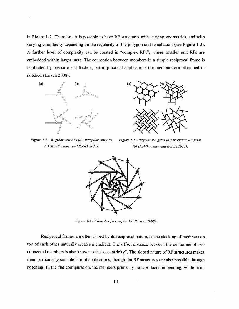
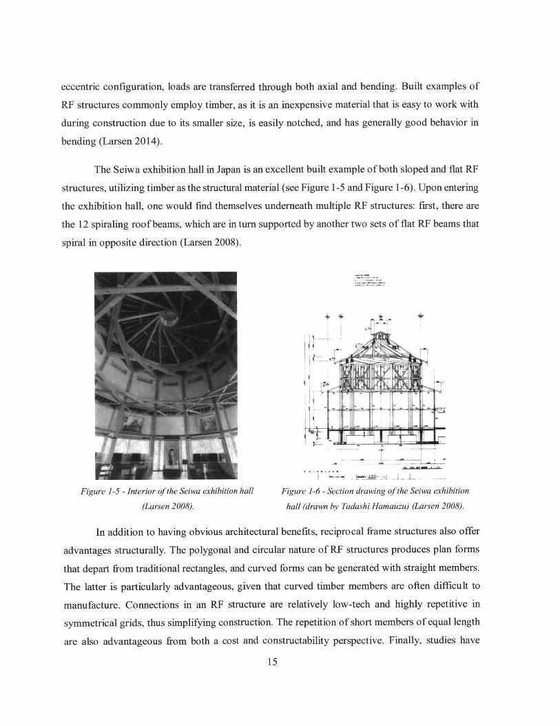
in Figure 1-2. Therefore, it is possible to have RF structures with varying geometries, and with
varying complexity depending on the regularity of the polygon and tessellation (see Figure 1-2).
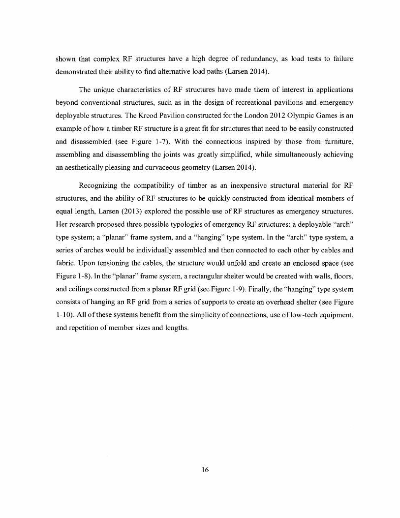
A further level of complexity can be created in "complex Rs", where smaller unit RFs are
embedded within larger units. The connection between members in a simple reciprocal frame is
facilitated by pressure and friction, but in practical applications the members are often tied or
notched (Larsen 2008).
(a) (b) (a) (b)
Figure 1-2 - Regular unit RFs (a); Irregular unit RFs Figure 1-3 - Regular RF grids (a); Irregular RF grids
(b) (Kohlhammer and Kotnik 2011). (b) (Kohlhammer and Kotnik 2011).
Figure 1-4 - Example of a complex RF (Larsen 2008).
Reciprocal frames are often sloped by its reciprocal nature, as the stacking of members on
top of each other naturally creates a gradient. The offset distance between the centerline of two
connected members is also known as the "eccentricity". The sloped nature of RF structures makes
them particularly suitable in roof applications, though flat RF structures are also possible through
notching. In the flat configuration, the members primarily transfer loads in bending, while in an
14
eccentric configuration, loads are transferred through both axial and bending. Built examples of
RF structures commonly employ timber, as it is an inexpensive material that is easy to work with
during construction due to its smaller size, is easily notched, and has generally good behavior in
bending (Larsen 2014).
The Seiwa exhibition hall in Japan is an excellent built example of both sloped and flat RF
structures, utilizing timber as the structural material (see Figure 1-5 and Figure 1-6). Upon entering
the exhibition hall, one would find themselves underneath multiple RF structures: first, there are
the 12 spiraling roof beams, which are in turn supported by another two sets of flat RF beams that
spiral in opposite direction (Larsen 2008).
Figure 1-5 - Interior of the Seiwa exhibition hall
(Larsen 2008).
Figure 1-6 - Section drawing of the Seiwa exhibition
hall (drawn by Tadashi Hanauzu) (Larsen 2008).
In addition to having obvious architectural benefits, reciprocal frame structures also offer
advantages structurally. The polygonal and circular nature of RF structures produces plan forms
that depart from traditional rectangles, and curved forms can be generated with straight members.
The latter is particularly advantageous, given that curved timber members are often difficult to
manufacture. Connections in an RF structure are relatively low-tech and highly repetitive in
symmetrical grids, thus simplifying construction. The repetition of short members of equal length
are also advantageous from both a cost and constructability perspective. Finally, studies have
15
shown that complex RF structures have a high degree of redundancy, as load tests to failure
demonstrated their ability to find alternative load paths (Larsen 2014).
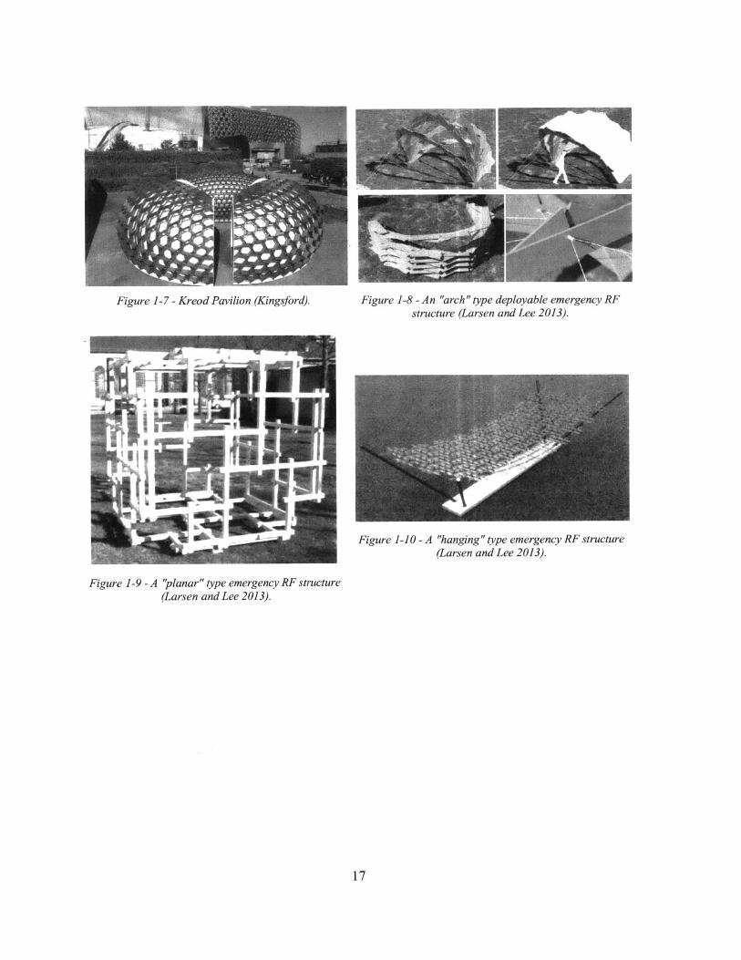
The unique characteristics of RF structures have made them of interest in applications
beyond conventional structures, such as in the design of recreational pavilions and emergency
deployable structures. The Kreod Pavilion constructed for the London 2012 Olympic Games is an
example of how a timber RF structure is a great fit for structures that need to be easily constructed
and disassembled (see Figure 1-7). With the connections inspired by those from furniture,
assembling and disassembling the joints was greatly simplified, while simultaneously achieving
an aesthetically pleasing and curvaceous geometry (Larsen 2014).
Recognizing the compatibility of timber as an inexpensive structural material for RF
structures, and the ability of RF structures to be quickly constructed from identical members of
equal length, Larsen (2013) explored the possible use of RF structures as emergency structures.
Her research proposed three possible typologies of emergency RF structures: a deployable "arch"
type system; a "planar" frame system, and a "hanging" type system. In the "arch" type system, a
series of arches would be individually assembled and then connected to each other by cables and
fabric. Upon tensioning the cables, the structure would unfold and create an enclosed space (see
Figure 1-8). In the "planar" frame system, a rectangular shelter would be created with walls, floors,
and ceilings constructed from a planar RF grid (see Figure 1-9). Finally, the "hanging" type system
consists of hanging an RF grid from a series of supports to create an overhead shelter (see Figure
1-10). All of these systems benefit from the simplicity of connections, use of low-tech equipment,
and repetition of member sizes and lengths.
16
k,~
ir7V-~i
LA~~ -
Figure 1-9 - A "planar" type emergency RF structure(Larsen and Lee 2013).
Figure 1-8 - An "arch" ype deployable emergency RFstructure (Larsen and Lee 2013).
2 V
Figure 1-10 - A "hanging" type emergencv RF structure(Larsen and Lee 2013).
17
Figure 1-7 - Kreod Pavilion (Kingsford)
- -
,A
1.2. Problem Statement
The topic of structural optimization has garnered interest in recent years, which can be attributed
to the increased awareness of environmental sustainability in structural design, and how efficient
structures can reduce the carbon footprint through minimizing material quantities. The latter is
particularly powerful when faced with the statistic that more than 50% of a structure's total carbon
footprint during its lifetime can be the embodied carbon of its structure (Kaethner and Burridge
2012).
Given that RF structures can come in a wide variety of topologies, geometries, and forms,
what constitutes as an "optimal" RF structure is not well understood yet. The motivation behind
this topic is to benefit the practical application of RF grids as a floor or roof framing structure,
with the aim of generating results that will serve as useful rules of thumb for designers who are
contemplating the use of a planar RF grid in their structure. Therefore, the question is whether
there is a particular RF grid geometry for the triangular topology that is optimal across both
symmetric and asymmetric load cases.
This thesis continues research on how geometry impacts the structural efficiency of an RF
structure. The thesis focusses on a planar RF grid with a triangular topology, which consists of 3
members at the unit RF level. The goal is to determine what the optimal geometry is for various
load cases, and whether this optimal would vary greatly across the different load cases. The
geometry of an RF grid is defmed by two variables; the rotation angle of the members, which
dictates the size of the engagement window (see Figure 1-11), and the density of the grid, which
dictates the number of members comprising the grid. The three smallest possible grid densities are
explored: the first with 12 members in total, or 6 unit RFs; the second with 42 members (24 unit
RFs), and the third with 156 members (96 unit RFs). In this thesis, the grid densities are referred
to by the number of unit RFs they consist of (i.e. N = 6, N = 24, N = 96).
The load cases considered have been chosen based on possible real-world loading
scenarios, on the assumption that the RF structure will be supporting a flat roof or floor surface.
Both symmetric and asymmetric load cases are analyzed, which are summarized in Table 1-1 and
represented in Figure 1-12. All load cases include the self-weight of the members. The area loads
are applied on the members as discretized point loads and distributed by tributary area, and the
self-weight is applied as a uniform line load on the members. The joints between members are
18

assumed to be notched connections and therefore are pin connections. The boundary support
conditions are rollers, except for one pin for lateral resistance. Lateral loads and torsion are not
considered in this thesis, and only linear elastic behavior is assumed in the analysis. Since the grid
is planar, the primary structural action is in bending.
, V
A
j
~
-. 4
W
7< \ <-~
VFigure 1-11 - N = 24 grids with varying rotation angles.
The engagement window is highlighted with a dotted triangle.
Symmetric Load Cases LC 1. Uniform area load + self-weight
LC 2. Uniform area load with concentrated load at center + self-
weight
Asymmetric Load Cases LC 3. Uniform area load with concentrated load at midpoint
between center and support + self-weight
LC 4. Uniform area load on half of grid + self-weight
Table 1-I - Sumnaiv of load cases.
LC 2 LC 3 LC 4
Figure 1-12 - Schematic of applied loads, as shown on the N = 24 Grid.Shaded area indicates extent of area load; point indicates location of concentrated load.
19
____________ ________ I
LC 1

20
2. Literature Review
Despite being a structural system that has been around for centuries, reciprocal frame structures
have not been commonly adopted in practice. Researchers suggest that it is likely because their
structural behavior was never well understood. Structural systems are often selected for a given
design problem on the basis of appropriateness given the loading conditions, span requirements,
and architectural goals. As Parigi & Kirkegaard (2013a) note, it is unclear under what
circumstances would a reciprocal frame be a good fit as a structural system. Therefore, several
studies in recent decades have sought to better understand the structural behavior of RF structures.
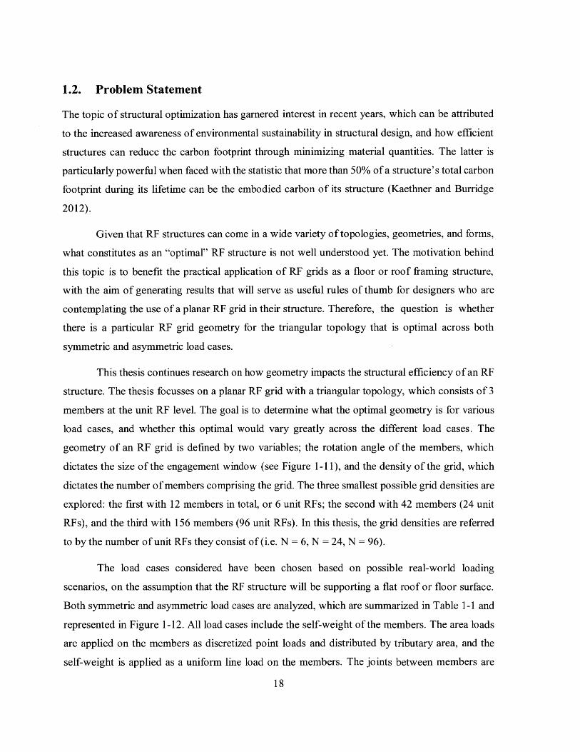
Gelez, Aubry & Vaudeville (2011) studied planar RF grids with the rectangular topology,
with the aim of better understanding their structural behavior in order to facilitate their design. In
their study, they proposed two mathematical formulas pertaining to the structural analysis of a
given RF grid: one that provides the value of maximum bending moment, and another that provides
the value of bending moment and deflection at any location. The loads applied were vertical point
loads (see Figure 2-1). They also compared the structural behavior of the RF grid to an equivalent
flat grid, and found that the RF grid was not competitive with respect to bending moments and
deflections. However, the distribution of bending moments was more even in the RF grid, and
when subjected to an irregular perimeter geometry, the RF grid performed better in terms of
distributing the support reactions (see Figure 2-2). Therefore, they concluded that despite the
disadvantages of the rectangular RF grid in terms of required stiffness and strength, there are
benefits to their application in certain situations that require irregular perimeters, and low
sensitivity to settlements, local thermal loads, or global thermal loads.
I Reactions Bending moments
Figure 2-1 - Example of an RF grid with rectangulartopology studied by Gelez et al (2011).
21
Figure 2-2 - Comparison between an RF grid and aregular grid/for an irregular perimeter (Ge/eZ, Auby,
and Vaudeville 2011).
-I-- --- j
z
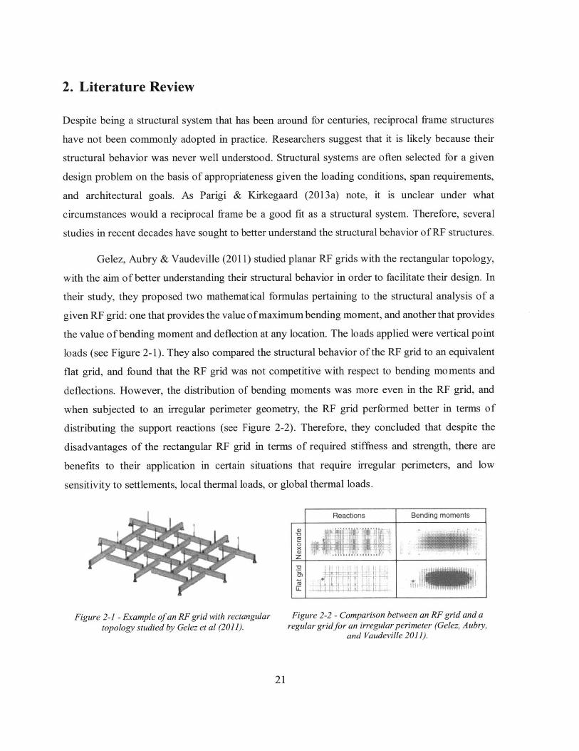
Parigi & Kirkegaard (2013a) studied the structural efficiency of various 2D and 3D RF
configurations with the triangular topology. Their research is the most relevant to this thesis, as
they were also interested in exploring the effect of geometric parameters on structural
performance. Parigi & Kirkegaard studied 8 different RF geometries, both in 2D as flat grids and
also in 3D by varying the eccentricities of the members (see Figure 2-3). The structural efficiency
of each was taken as the value of maximum stress and displacement, and the two load cases
consisted of a uniform line load
each member (asymmetric).
Ile
on each member (symmetric), or a uniform line load on half of
1-~
'74--I
r-
>~
r~-~
Figure 2-3 - Planar RFgrid configurations studied by Parigi and Kirkegaard (2013a).
Although this thesis is similar in principle to the research performed by Parigi &
Kirkegaard (2013a), it addresses some of the points for future work that was suggested in their
research, and therefore differs by a few key aspects. The first is the use of global values such as
total strain energy in assessing the structural performance, as opposed to the local values of
maximum stress and displacement. Using global values would better capture the efficiency of the
structure as a whole, because it would account for the contributions each member has in the
performance of the grid. A downside to considering simply the value of maximum stress in the
grid is that it only reflects what is happening at a single member level, and does not reflect the
stress distribution among other members. Therefore, the evaluation of structural efficiency
22
utilizing the total strain energy is expected to produce more representative results on the
performance of the entire structure.
The second suggested point for future work that is addressed in this thesis is the
consideration for pin connections between elements. In their research, Parigi & Kirkegaard
(2013a) only modelled the joints between members as fixed, which would unlikely be the case in
reality as there would be some rotational freedom between the members.
A final difference in the methodology is the modelling of the loads. In this thesis, load
cases that represent possible loading scenarios in reality are considered, as the structure is
considered to be a hypothetical structural floor framing system. The loads are therefore distributed
onto the members by tributary area, which contrasts with previous work as the members would
receive non-uniform linear loads.
Kirkegaard and Parigi (2013b) also explored the topic of robustness for reciprocal frame
structures. They hypothesized that RF structures would be prone to progressive collapse due to the
mutually supporting nature of the members; however, the results from their research proved
otherwise. They found that RF structures are capable of redistributing the loads when subject to a
loss of a member or a support, but that the sensitivity of a structure to a failure depends on where
the failed member occurs. With the requirement of robustness being specified in most building
codes across the globe, the application of an RF as a structural system could therefore constitute
as a method of addressing this requirement, since it involves "selecting a structural form that can
survive the accidental removal of an individual member or limited part of the structure" - one of
the robust design principles outlined in the Eurocode.
23

24
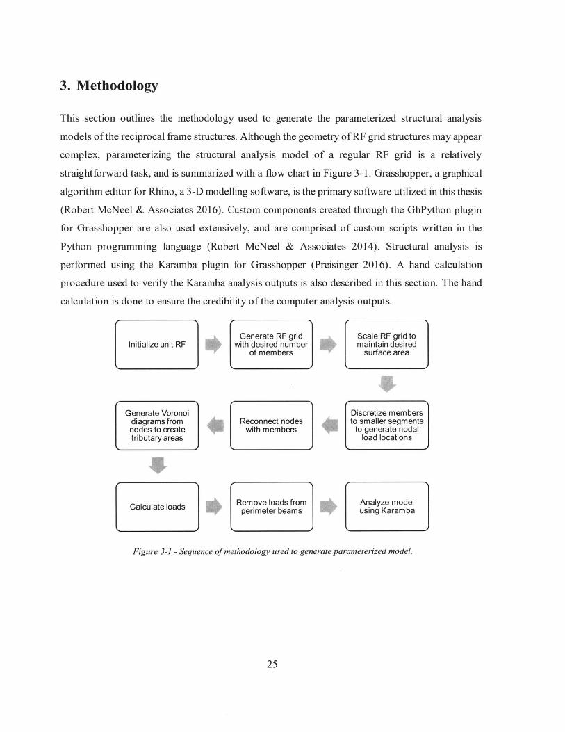
3. Methodology
This section outlines the methodology used to generate the parameterized structural analysis
models of the reciprocal frame structures. Although the geometry of RF grid structures may appear
complex, parameterizing the structural analysis model of a regular RF grid is a relatively
straightforward task, and is summarized with a flow chart in Figure 3-1. Grasshopper, a graphical
algorithm editor for Rhino, a 3-D modelling software, is the primary software utilized in this thesis
(Robert McNeel & Associates 2016). Custom components created through the GhPython plugin
for Grasshopper are also used extensively, and are comprised of custom scripts written in the
Python programming language (Robert McNeel & Associates 2014). Structural analysis is
performed using the Karamba plugin for Grasshopper (Preisinger 2016). A hand calculation
procedure used to verify the Karamba analysis outputs is also described in this section. The hand
calculation is done to ensure the credibility of the computer analysis outputs.
Initialize unit RF
Generate Voronoidiagrams fromnodes to createtributary areas
Calculate loads
Generate RF gridwith desired number
of members
Reconnect nodeswith members
Remove loads fromperimeter beams
Scale RF grid tomaintain desired
surface area
Discretize membersto smaller segments
to generate nodalload locations
Analyze modelusing Karamba
Figure 3-1 - Sequence of methodologv used to generate parameterized model.
25
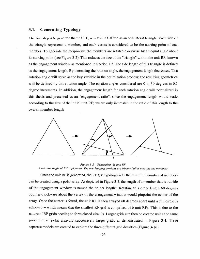
3.1. Generating Typology
The first step is to generate the unit RF, which is initialized as an equilateral triangle. Each side of
the triangle represents a member, and each vertex is considered to be the starting point of one
member. To generate the reciprocity, the members are rotated clockwise by an equal angle about
its starting point (see Figure 3-2). This reduces the size of the "triangle" within the unit RF, known
as the engagement window as mentioned in Section 1.2. The side length of this triangle is defined
as the engagement length. By increasing the rotation angle, the engagement length decreases. This
rotation angle will serve as the key variable in the optimization process; the resulting geometries
will be defined by this rotation angle. The rotation angles considered are 0 to 30 degrees in 0.1
degree increments. In addition, the engagement length for each rotation angle will normalized in
this thesis and presented as an "engagement ratio", since the engagement length would scale
according to the size of the initial unit RF; we are only interested in the ratio of this length to the
overall member length.
Figure 3-2 - Generating the unit RF.
A rotation angle of 150 is pictured The overhanging portions are trimmed after rotating the members.
Once the unit RF is generated, the RF grid typology with the minimum number of members
can be created using a polar array. As depicted in Figure 3-3, the length of a member that is outside
of the engagement window is named the "outer length". Rotating this outer length 60 degrees
counter-clockwise about the vertex of the engagement window would pinpoint the center of the
array. Once the center is found, the unit RF is then arrayed 60 degrees apart until a full circle is
achieved - which means that the smallest RF grid is comprised of 6 unit RFs. This is due to the
nature of RF grids needing to form closed circuits. Larger grids can then be created using the same
procedure of polar arraying successively larger grids, as demonstrated in Figure 3-4. Three
separate models are created to explore the three different grid densities (Figure 3-16).
26

A)40
Figure 3-3 - Diagrammatic procedure of generating the N = 6 Grid.A unit RF with the "outer length " highlighted (left,): Outer length rotated by 60 degrees to get center of array'
(center), Grid generation following polar array (right).
7" 1/
W /
/
-"-V
-. ,I " ~/ ~ - -
~*'-4 ',
' ~
Figure 3-4 - Diagrammatic procedure of generating the N = 24 Grid.
The total number of RF units (N) in a grid can be calculated from Equation 1, based on the
number of rotational arrays (n) needed to attain the grid. For example, the next grid size up from
the base N = 6 grid would be N = 24, since two arrays are needed (first to generate the N = 6 grid,
and second to generate the N = 24). The N = 96 grid is therefore generated from three arrays.
N = 6 * 4 l1 (1)
Due to the self-supporting nature of a reciprocal frame, a connection point between two
members result in one of the members being supported or supporting the other. In an RE grid with
triangular topology, the supported vs. supporting conditions for each connection point in a given
member is straightforward, as there are only two types of members. An interior member is always
supported on its ends and supporting two along its span, and the exterior members connecting to
the supports are always supported on both ends and supporting one member along its span (see
Figure 3-5). A plan view schematic of the supported vs. supporting conditions at each joint is
shown in Figure 3-6. For any given vertical load on a member, the load will be resisted in bending
27
- I
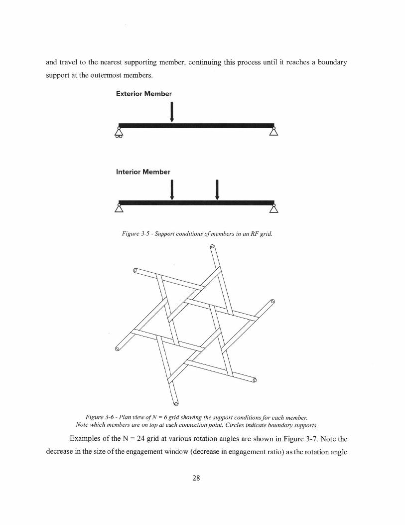
and travel to the nearest supporting member, continuing this process until it reaches a boundary
support at the outermost members.
Exterior Member
Interior Member
Figure 3-5 - Support conditions of members in an RF grid.
Figure 3-6 - Plan view of N = 6 grid showing the support conditions for each member.Note which members are on top at each connection point. Circles indicate boundary supports.
Examples of the N = 24 grid at various rotation angles are shown in Figure 3-7. Note the
decrease in the size of the engagement window (decrease in engagement ratio) as the rotation angle
28
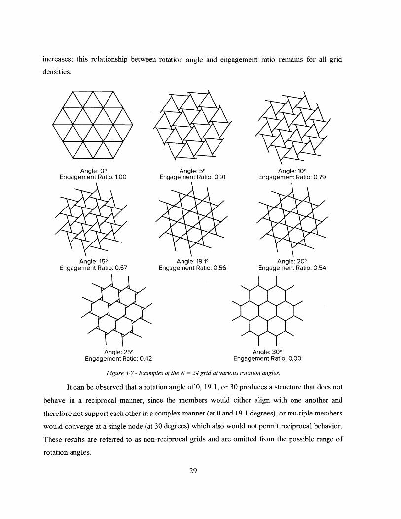
increases; this relationship
densities.
between rotation angle and engagement ratio remains for all grid
Angle: 00Engagement Ratio: 1.00
Angle: 150Engagement Ratio: 0.67
Angle: 50Engagement Ratio: 0.91
Angle: 19.10Engagement Ratio: 0.56
Angle: 100Engagement Ratio: 0.79
Angle: 200Engagement Ratio: 0.54
Angle: 250 Angle: 300Engagement Ratio: 0.42 Engagement Ratio: 0.00
Figure 3-7 - Examples of the N = 24 grid at various rotation angles.
It can be observed that a rotation angle of 0, 19.1, or 30 produces a structure that does not
behave in a reciprocal manner, since the members would either align with one another and
therefore not support each other in a complex manner (at 0 and 19.1 degrees), or multiple members
would converge at a single node (at 30 degrees) which also would not permit reciprocal behavior.
These results are referred to as non-reciprocal grids and are omitted from the possible range of
rotation angles.
29
0
3.2. Maintaining Desired Surface Area
The third step is to scale the RF grid to obtain the desired surface area of the floor or roof framing
structure. This is because for a given initial length of members at the unit RF level, the surface
area of the RF grid changes as the rotation angle changes. Therefore in order to maintain a constant
coverage area, the parameterized model needs to be scaled to the correct size for each rotation
angle, after the polar arraying process.
In this thesis, the surface area is the area bounded by the perimeter beams (see Figure 3-8).
The area is taken to be the equivalent of a circular space with a radius of 5 m, which leads to an
area of 78.54 m2 . The resulting span is approximately 10 m. The surface area is maintained across
all grid densities in order to compare the effect of grid density for a fixed floor or roof area.
Figure 3-8 - Diagram indicating the surface area of a grid (shaded).
3.3. Discretization of Members for Loading
The fourth step is the discretization of members to smaller segments. This step is needed due to
complications in utilizing the Mesh Load component in Karamba to translate area loads into
distributed line loads on members (Preisinger 2016). As a result, distributed loads are discretized
as closely spaced point loads. In order to apply point loads along the length of a member in
Karamba, a physical node must exist at the point load location. Hence, the members are divided
into segments of equal length to generate the nodes, and a custom component is coded to re-draw
the members between the nodes. The node spacing is set to 0.1 m, as it was found that nodes too
close together could lead to bugs when generating Voronoi diagrams, which are needed for proper
calculation of the tributary areas. The bug causes the tributary areas to overlap, which leads to an
improper calculation of the tributary areas (see Figure 3-9).
30
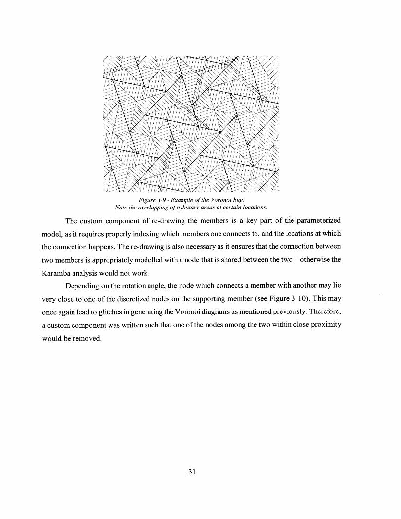
Figure 3-9 -Example of the Voronoi bug.Note the overlapping of tributary areas at certain locations.
The custom component of re-drawing the members is a key part of thie parameterized
model, as it requires properly indexing which members one connects to, and the locations at which
the connection happens. The re-drawing is also necessary as it ensures that the connection between
two members is appropriately modelled with a node that is shared between the two - otherwise the
Karamba analysis would not work.
Depending on the rotation angle, the node which connects a member with another may lie
very close to one of the discretized nodes on the supporting member (see Figure 3-10). This may
once again lead to glitches in generating the Voronoi diagrams as mentioned previously. Therefore,
a custom component was written such that one of the nodes among the two within close proximity
would be removed.
31
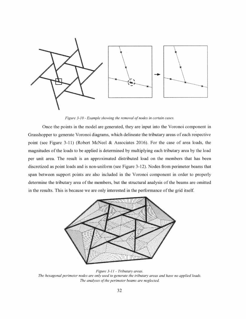
Figure 3-10 - Example showing the removal of nodes in certain cases.
Once the points in the model are generated, they are input into the Voronoi component in
Grasshopper to generate Voronoi diagrams, which delineate the tributary areas of each respective
point (see Figure 3-11) (Robert McNeel & Associates 2016). For the case of area loads, the
magnitudes of the loads to be applied is determined by multiplying each tributary area by the load
per unit area. The result is an approximated distributed load on the members that has been
discretized as point loads and is non-uniform (see Figure 3-12). Nodes from perimeter beams that
span between support points are also included in the Voronoi component in order to properly
determine the tributary area of the members, but the structural analysis of the beams are omitted
in the results. This is because we are only interested in the performance of the grid itself.
Figure 3-11 - Tributarv areas.The hexagonal perimeter nodes are on/y ised to generate the tributarv areas and have no applied loads.
The analvses of the perimeter beams are neglected.
32
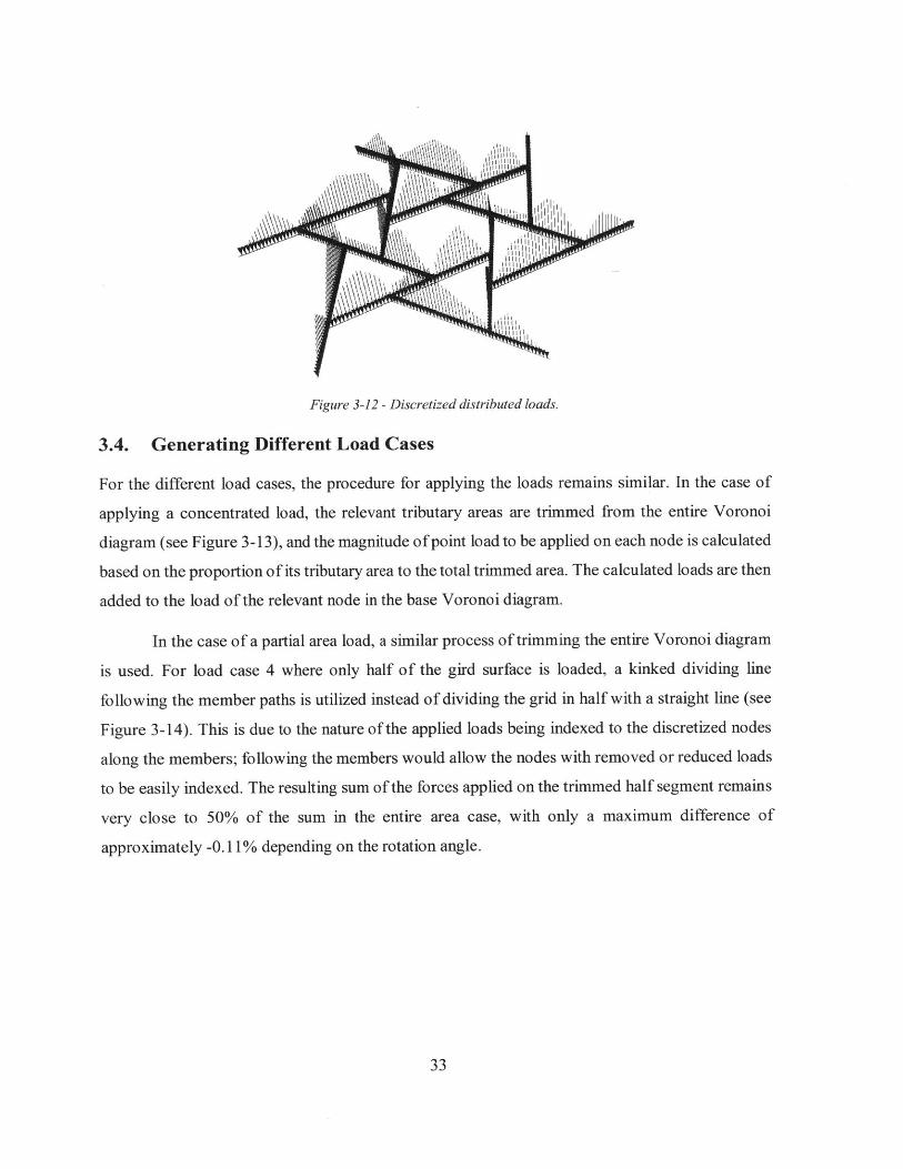
Figure 3-12 - Discretized distributed loads.
3.4. Generating Different Load Cases
For the different load cases, the procedure for applying the loads remains similar. In the case of
applying a concentrated load, the relevant tributary areas are trimmed from the entire Voronoi
diagram (see Figure 3-13), and the magnitude of point load to be applied on each node is calculated
based on the proportion of its tributary area to the total trimmed area. The calculated loads are then
added to the load of the relevant node in the base Voronoi diagram.
In the case of a partial area load, a similar process of trimming the entire Voronoi diagram
is used. For load case 4 where only half of the gird surface is loaded, a kinked dividing line
following the member paths is utilized instead of dividing the grid in half with a straight line (see
Figure 3-14). This is due to the nature of the applied loads being indexed to the discretized nodes
along the members; following the members would allow the nodes with removed or reduced loads
to be easily indexed. The resulting sum of the forces applied on the trimmed half segment remains
very close to 50% of the sum in the entire area case, with only a maximum difference of
approximately -0.11% depending on the rotation angle.
33
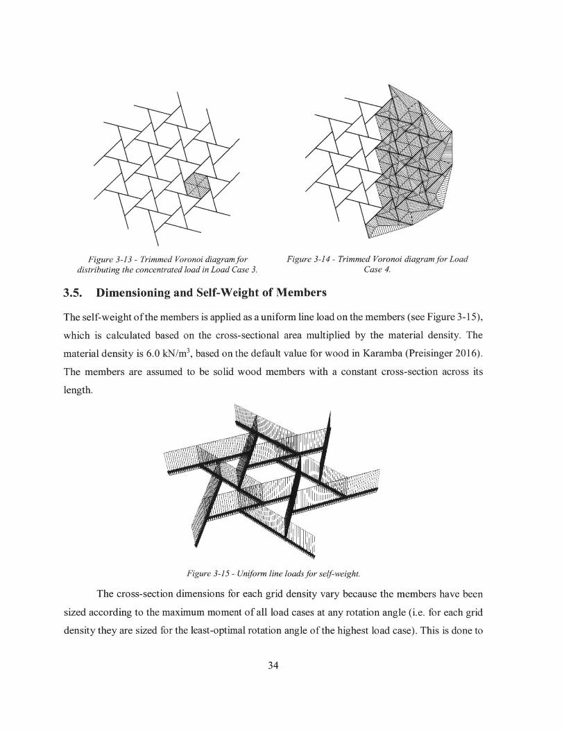
Figure 3-13 - Trimmed Voronoi diagram ftrdistributing the concentrated load in Load Case 3.
Figure 3-14 - Trimmed Voronoi diagram tor LoadCase 4.
3.5. Dimensioning and Self-Weight of Members
The self-weight ofthe members is applied as a uniform line load on the members (see Figure 3-15),
which is calculated based on the cross-sectional area multiplied by the material density. The
material density is 6.0 kN/m 3, based on the default value for wood in Karamba (Preisinger 2016).
The members are assumed to be solid wood members with a constant cross-section across its
length.
Figiurc 3-15 - Uniform line loads for self-weight.
The cross-section dimensions for each grid density vary because the members have been
sized according to the maximum moment of all load cases at any rotation angle (i.e. for each grid
density they are sized for the least-optimal rotation angle of the highest load case). This is done to
34
-I
avoid errors in the computer analysis, as the results could be erroneous if the utilization of a
member (which is primarily due to bending) greatly exceeds 1.0. Another benefit to maintaining a
constant cross-section across all rotation angles is that the optimization process can be linearized,
as the "optimal" would only be defined by geometry and not also the self-weight.
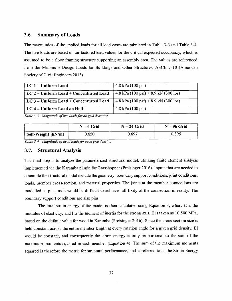
The member sizes for each grid density are shown in Table 3-1. The width has been held
constant, while the depth changes according to the maximum moment for any rotation angle in
load case 2 (the highest loading demand). Therefore, the members have been sized according to
strength requirements. The required width is calculated from Equation 2, where Mr is the required
moment resistance, Fy is the tensile yield stress of the material, and b is the member width. The
tensile yield stress is 13 MPa, based on the default value for wood in Karamba (Preisinger 2016).
This value corresponds roughly to the tensile strength parallel to the grain of a type C22 softwood
species in EN 338-2003, which contains the strength properties of structural timber (European
Committee for Standardization 2003). The cross-section size is the same across the entire length
of the members.
6 * Mr
h= F r* (2)
N = 6 Grid N = 24 Grid N = 96 Grid
Member Width [in] 6 6 6
Member Height [in] 28 30 17
Table 3-1 - Member dimensions for each grid density.
As it is found that the bending moment tends to increase greatly towards higher rotation
angles for the two denser grids, the maximum moment used for sizing is capped off at around 27
degrees, beyond which it increases much greater than the typical increment.
Since the chosen dimensions have an impact on the self-weight of the members, which in
turn impacts the magnitude of the bending moments in the members, the results could be affected
as the sizing for each rotation angle is not optimized for its own bending demand (i.e. an
unnecessarily high self-weight moment could skew the efficiency of a geometric configuration).
To ensure this is not the case, the member depth for the rotation angle with the lowest maximum
bending moment in load case 2 (4.7 degrees) was optimized for its own maximum moment, and
35
this value was compared with its maximum moment under the non-optimized dimension. Load
case 2 is utilized because it is the expected worst-case. It would not be rational to optimize a
member under load case 4 since it would have lower moments.
The result in Table 3-2 shows that the self-weight has minimal effect on the maximum
moment for a given rotation angle, as the difference in moments between the optimized and non-
optimized dimensions is less than 10%. This means that the size of the members has a small impact
on the optimum angle. Although the member depths appear large, they are somewhat arbitrary as
they are affected by the defined span and the material properties. Similar results would be obtained
with smaller sections if the span was reduced or if a different species of timber was used.
Non-Optimally Sized Optimally Sized Difference
Member Depth [in] 30 17
Max. Moment (without 51.3 51.3
self-weight) [kNm]
Max. Moment (incl. self- 61.1 56.9 -7.47%
weight) [kNm]
Table 3-2 - Effect of self-weight on the max. bending moment at 4.7 degrees (N = 24 grid).
Finally, although the parameterized structural model is a stick model where the members
have been idealized as lines without thickness, it is important to note the implications of member
width on possible geometries. For certain rotation angles where the connection points are in close
proximity, the member width must be taken into account in reality as the members cannot overlap.
However, since the actual member widths have been arbitrarily chosen in this thesis and could
vary in reality, the rotation angles leading to an overlapping of members are still included in the
results. Overlapping does not negatively affect the analysis results since the analysis model is a
stick model - the cross-sections are only used to compute strength, deflections, and weight.
36
3.6. Summary of Loads
The magnitudes of the applied loads for all load cases are tabulated in Table 3-3 and Table 3-4.
The live loads are based on un-factored load values for the critical expected occupancy, which is
assumed to be a floor framing structure supporting an assembly area. The values are referenced
from the Minimum Design Loads for Buildings and Other Structures, ASCE 7-10 (American
Society of Civil Engineers 2013).
LC 1 - Uniform Load 4.8 kPa (100 psf)
LC 2 - Uniform Load + Concentrated Load 4.8 kPa (100 psf) + 8.9 kN (300 lbs)
LC 3 - Uniform Load + Concentrated Load 4.8 kPa (100 psf) + 8.9 kN (300 lbs)
LC 4 - Uniform Load on Half 4.8 kPa (100 pst)
Table 3-3 - Magnitude of live loads for all grid densities.
N = 6 Grid N = 24 Grid N = 96 Grid
Self-Weight [kN/m] 0.650 0.697 .0.395
Table 3-4 - Magnitude of dead loads for each grid density.
3.7. Structural Analysis
The final step is to analyze the parameterized structural model, utilizing finite element analysis
implemented via the Karamba plugin for Grasshopper (Preisinger 2016). Inputs that are needed to
assemble the structural model include the geometry, boundary support conditions, joint conditions,
loads, member cross-section, and material properties. The joints at the member connections are
modelled as pins, as it would be difficult to achieve full fixity of the connection in reality. The
boundary support conditions are also pins.
The total strain energy of the model is then calculated using Equation 3, where E is the
modulus of elasticity, and I is the moment of inertia for the strong axis. E is taken as 10,500 MPa,
based on the default value for wood in Karamba (Preisinger 2016). Since the cross-section size is
held constant across the entire member length at every rotation angle for a given grid density, El
would be constant, and consequently the strain energy is only proportional to the sum of the
maximum moments squared in each member (Equation 4). The sum of the maximum moments
squared is therefore the metric for structural performance, and is referred to as the Strain Energy
37
Factor. It is independent of the material cross-section, and is solely dependent on geometry. Note
that a lower value for the Strain Energy Factor corresponds to a more efficient geometry.
Strain Energy = Mmax2
2EI
Strain Energy Factor = Mmax2
L
(3)
(4)
AIA
Figure 3-16 - Structural model of the 3 different grid densities.The arrows at the on the members indicate the support locations.
I
38
-A
3.8. Categorization of Member Types
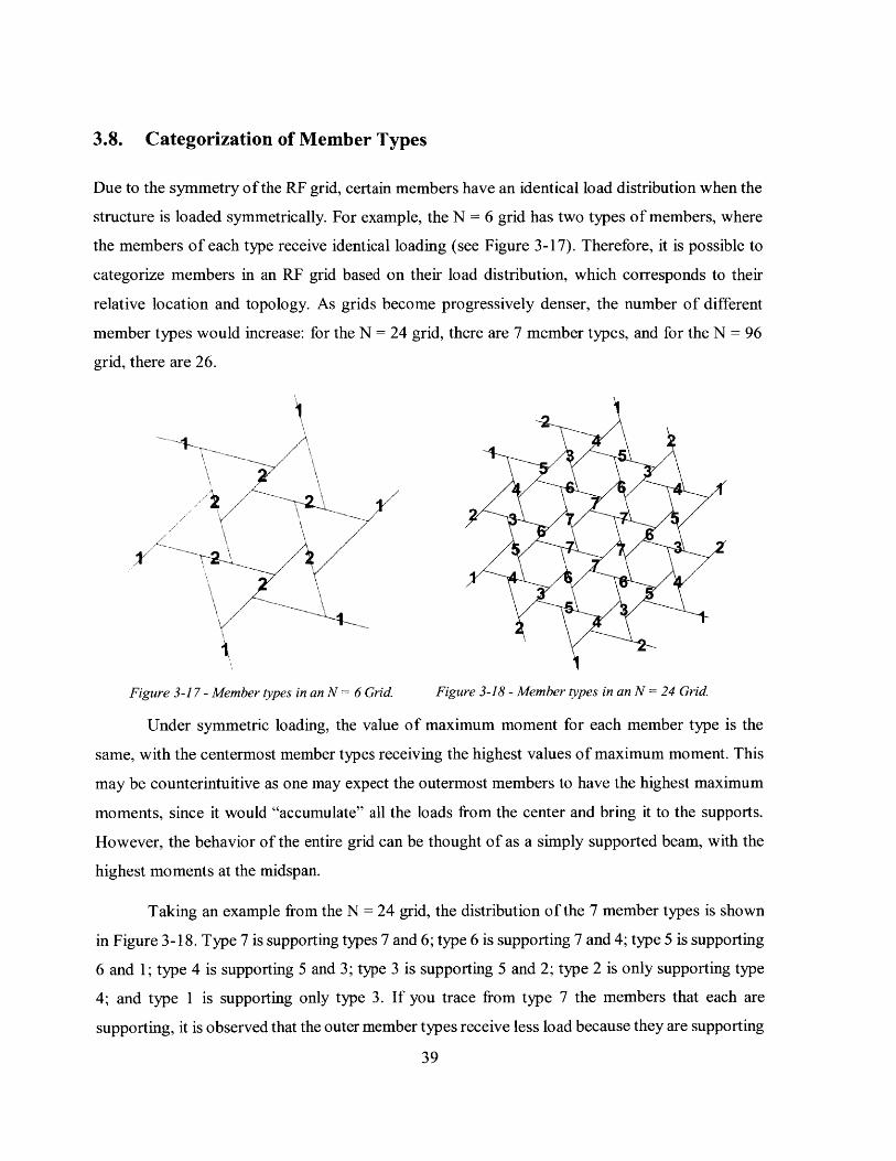
Due to the symmetry of the RF grid, certain members have an identical load distribution when the
structure is loaded symmetrically. For example, the N = 6 grid has two types of members, where
the members of each type receive identical loading (see Figure 3-17). Therefore, it is possible to
categorize members in an RF grid based on their load distribution, which corresponds to their
relative location and topology. As grids become progressively denser, the number of different
member types would increase: for the N = 24 grid, there are 7 member types, and for the N = 96
grid, there are 26.
I
/
-7
1' /
I
/
Figure 3-17- Member types in an N 6 Grid. Figure 3-18 - Member types in an N = 24 Grid.
Under symmetric loading, the value of maximum moment for each member type is the
same, with the centermost member types receiving the highest values of maximum moment. This
may be counterintuitive as one may expect the outermost members to have the highest maximum
moments, since it would "accumulate" all the loads from the center and bring it to the supports.
However, the behavior of the entire grid can be thought of as a simply supported beam, with the
highest moments at the midspan.
Taking an example from the N = 24 grid, the distribution of the 7 member types is shown
in Figure 3-18. Type 7 is supporting types 7 and 6; type 6 is supporting 7 and 4; type 5 is supporting
6 and 1; type 4 is supporting 5 and 3; type 3 is supporting 5 and 2; type 2 is only supporting type
4; and type 1 is supporting only type 3. If you trace from type 7 the members that each are
supporting, it is observed that the outer member types receive less load because they are supporting
39
members that carry less load. Due to symmetry, a majority of members have identical tributary
areas and are supporting two members each, with the exception of the outermost members
connected to the support points (type 1 and 2) - they are only supporting one member and have a
different tributary area. As a consequence, members that support member type 1 and 2 (types 3
and 5) would subsequently receive less load than those further away from the outside, and in that
sense the "accumulation" of loads is actually reversed in the case of an RF grid.
The ability to categorize members based on their loading distribution can be beneficial in
terms of generating material savings, as the member size can be optimized based on their expected
maximum load under symmetric and asymmetric loading.
3.9. Hand Calculation Verification
To verify the structural analysis results generated by the Karamba plugin, a hand calculation using
Excel is performed (Microsoft 2016). As we are only interested in verifying the accuracy of the
numerical results generated by the software, the simplest N = 6 grid with the uniform area load
(neglecting self-weight) is chosen as the case to verify against. The values that are verified against
the computer model are the Strain Energy Factor, and the values of maximum moment and shear.
Since the N 6 grid only has two member types (refer to Figure 3-17), only two members need to
be analyzed in Excel as the remaining members would be identical in behavior to one of the two.
The first step is to import from Grasshopper the tributary areas for each node on the two
members. The magnitude of the force on each node is then calculated by multiplying the areas by
the applied area load. Type 1 members have 3 unknown forces, and type 2 members have 4
unknown forces (see Figure 3-19). The type 1 member is analyzed first as it is statically
determinate: one of the unknowns is the reaction force (Ay), which can be solved due to symmetry
(each reaction is equal to the total vertical force on the grid divided by the six supports). Therefore,
two equations of equilibrium can be used to solve for all the remaining forces; sum of moments
about point B to solve for Cy (Equation 5), and sum of vertical forces to solve for By (Equation 6).
- j(Applied Loads * Moment Arms to B) - (A, * Length AB) (5)Length BC
By = -(AAy +Cy - Applied Loads) (6)
40
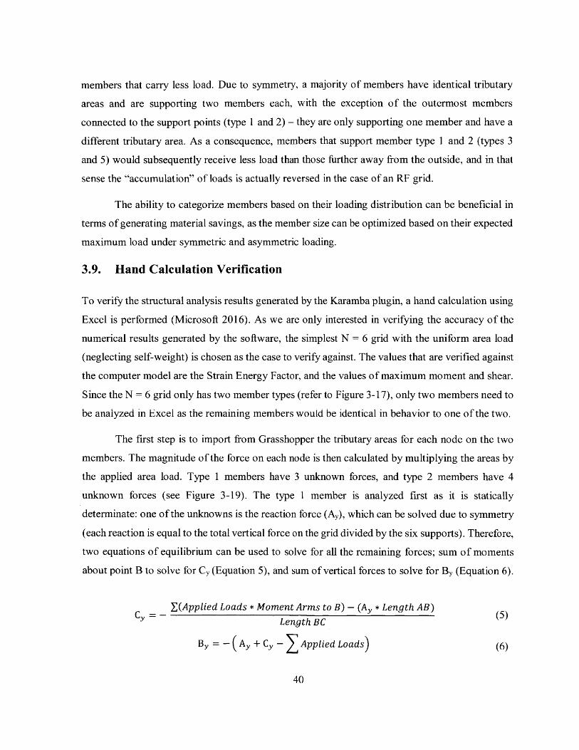
Type I
IA B C
Ay Cy
Type 2 Cy Dy
I B
C D EI
Figure 3-19 - Unknown forces on the two member types.The known applied loads along the members are not shown for claritv.
Due to symmetry, the magnitude of the unknown Cy in member type 1 is equal to Cy in
member type 2: this reduces the unknowns in member type 2 to two (Dy, Ey) and enables us to
solve for the forces in a similar manner using Equations 7 and 8. After all the unknown forces are
resolved, the shear and moment values at each node can be calculated. The moment values are
then used to calculate the Strain Energy Factor in each member type, using Equation 2.
X(Applied Loads * Moment Arms to D) + (C, * Length CD) - (By * Length BD)
Length DE
D= - (By - C+ Ey - Applied Loads)
(7)
(8)
The results of the hand calculation are compared with the Karamba output in Table 3-5.
Since the difference in the comparison values remain under 10%, the numerical results produced
through the parameterized model can therefore be accepted with confidence. Refer to Appendix A
for the spreadsheet of the hand calculations.
Hand Calculation Karamba Analysis Difference
EMmax [kNm2I 2.17 x 10⁶ 2.30 x 10⁶ -6.18%
Maximum Moment [kNm] 106 110 -3.11%
Maximum Shear [kNI 67.5 68.2 -1.10%
Table 3-5 - Comparison of hand calculation with Karamba output.
41
-I,
3.10. Summary of Methodology
The methodology of creating the parameterized structural analysis models was first discussed. The
parameterization used Grasshopper, Karamba, and Rhino (Robert McNeel & Associates 2016,
Preisinger 2016). The first step was to initialize the unit RF, from which we generated the three
respective grid densities through a succession of polar arrays. The grids were then scaled to the
appropriate size in order to maintain a constant surface area. Next, the procedure detailing how the
member loads have been distributed based on tributary areas was described; this distribution of
loads is a key contribution of this thesis to the research of planar reciprocal frames and their
behavior under various load cases. The rationale behind the member sizing was discussed, and the
Strain Energy Factor was introduced as the metric of structural performance for each geometry.
Finally, a method of categorizing the members in an RF grid based on their load distribution and
topology was presented. The methodology section concluded with a hand calculation procedure
that was performed to verify the credibility of the Karamba analysis results.
42
4. Results
The general trend across all grid densities and load cases is that the more structurally efficient grids
are those with a smaller rotation angle, and therefore larger engagement length. A common pattern
is that the Strain Energy Factor initially decreases to a minimum at a rotation angle between 4 and
9 degrees, then increases for rotation angles beyond. Recall from Section 3.7 that a lower value
for the Strain Energy Factor corresponds to a greater efficiency. The exact value of rotation angle
at which the optimal structural performance exists varies between the different grid densities and
load cases.
It is important to note that the results from the structural analysis are based on several
assumptions. Buckling out of plane due to bending, and the effect of stress concentrations at the
joints due to the assumed notching of members are not considered. Since certain rotation angles
have joints that are closer together, the stress concentrations at these areas could have an effect on
the efficiency of the structure that is not captured in the strain energy.
4.1. Organization of Results Section
The first part of the results section discusses the removal of certain data points due to possible
errors from the structural analysis. The remaining sections summarize the analysis outputs, which
have been organized in two ways: first, by grid density (Sections 4.3 to 4.5), which enables the
comparison of results between load cases for a given density; and second by load case (Sections
4.6 to 4.9), which enables the comparison of results between grid densities for each load case.
Primary discussion of the results are included in Sections 4.3 to 4.5 under each grid density. All
presented graphs are scatter plots of the data points at each rotation angle. The results section
closes with a comparison of a particular RF grid geometry with a similar non-reciprocal grid.
4.2. Filtering of Results
Upon reviewing the data points across the possible range of rotation angles, results from certain
rotation angles were removed due to possible errors in the structural analysis.
The first errors are manifested through the member utilization: at small rotation angles for
the N = 6 grid, the maximum member utilization would jump to values beyond 1.0, with many at
3000 - despite the fact that the value of maximum moment for those angles are less than those at
43
a higher, less optimal rotation angle. Although the bending moments corresponding to these
erroneous utilization values appear to correlate with the trend of the moment values, these results
are omitted due to possible errors. A similar problem occurs at the upper limit of rotation angles.
In general, the glitch is not present between the rotation angles of 2 and 28 degrees. It is plausible
that extremely high (and obviously erroneous) shear values may be contributing to the errors, even
though the maximum shear utilization output by Karamba is still less than that of the bending
utilization.
The second group of errors are from the grids with removed nodes. Recalling Section 3.3,
certain rotation angles required the removal of closely spaced nodes in order to avoid problems
with the Voronoi diagrams. However, it is found that this removal of nodes adversely affects the
results, as it leads to a sharp decrease in the Strain Energy Factor, which does not follow the general
pattern. Strain Energy Factors from rotation angles before and after those that have removed nodes
correlate with the trend, which suggests that the values with the removed nodes cannot be trusted.
These results are therefore removed from the results.
Depending on the grid density, the locations where results have been removed vary. Since
the removed results represent a small portion of the total number of results, it is justified as it does
not significantly affect the results.
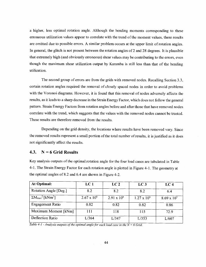
4.3. N = 6 Grid Results
Key analysis outputs of the optimal rotation angle for the four load cases are tabulated in Table
4-1. The Strain Energy Factor for each rotation angle is plotted in Figure 4-1. The geometry at
the optimal angles of 8.2 and 6.4 are shown in Figure 4-2.
At Optimal: LC 1 LC 2 LC 3 LC 4
Rotation Angle [Deg.] 8.2 8.2 8.2 6.4
IMmax 2 [kNm2 ] 2.67 x 10 6 2.91 x 10⁶ 1.27 x 10⁶ 8.69 x 10,
Engagement Ratio 0.82 0.82 0.82 0.86
Maximum Moment [kNm] 111 118 115 72.9
Deflection Ratio L/364 L/347 L/353 L/607
Table 4-1 - Analysis outputs of the optimal angle for each load case in the N = 6 Grid.
44
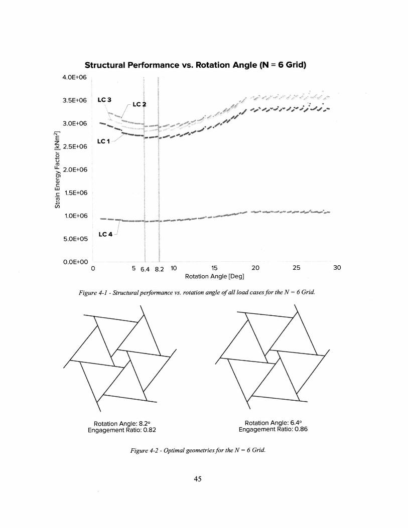
Structural Performance vs. Rotation Angle (N = 6 Grid)
4.OE+06
3.5E+06 LC 3LC 2
,00
LC 1
LC 4
5 6.4 8.2 10 15Rotation Angle [Deg]
Figure 4-1 - Structural performance vs. rotation angle of all load cases for the N = 6 Grid.
Rotation Angle: 8.20Engagement Ratio: 0.82
Rotation Angle: 6.40Engagement Ratio: 0.86
Figure 4-2 - Optimal geometries for the N = 6 Grid.
45
3.OE+06
z- 2.5E+060
2.OE+06
1.5E+06
1.0E+06
5.0E+05
0.0 E+000 20 25 30
-wo .",*.
4.3.1. Variation of Maximum Moments for N = 6 Grid
Figure 4-3 shows the value of maximum moments at each rotation angle for the two member types
under symmetric loading (load case 1). Figure 4-4 shows the member type maximum moments
under the most asymmetric loading (load case 4).
Maximum Moments for LC 1 (N = 6 Grid)
,z
a)E0
Q)~M
180160140120100
806040
20
0
Type 2
Type 1
0 5 8.2 10 15Rotation Angle [Deg.]
20 25 30
Figure 4-3 - LC I maximum moments for each member type in the N = 6 Grid.
Maximum Moments for LC 4 (N = 6 Grid)
15Rotation Angle [Deg.]
Figure 4-4 - LC 4 maximum moments for each member type in the N = 6 Grid.
46
140
120
100
80
60
40
20
Pfz
a)E0
0)
a)
Type 2
Type 1
00 5 6.4 10 20 25 30
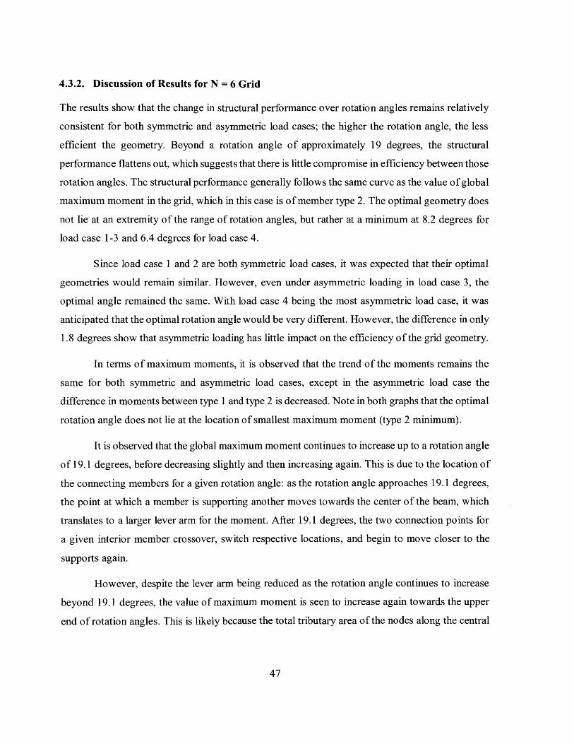
4.3.2. Discussion of Results for N = 6 Grid
The results show that the change in structural performance over rotation angles remains relatively
consistent for both symmetric and asymmetric load cases; the higher the rotation angle, the less
efficient the geometry. Beyond a rotation angle of approximately 19 degrees, the structural
performance flattens out, which suggests that there is little compromise in efficiency between those
rotation angles. The structural performance generally follows the same curve as the value of global
maximum moment in the grid, which in this case is of member type 2. The optimal geometry does
not lie at an extremity of the range of rotation angles, but rather at a minimum at 8.2 degrees for
load case 1-3 and 6.4 degrees for load case 4.
Since load case 1 and 2 are both symmetric load cases, it was expected that their optimal
geometries would remain similar. However, even under asymmetric loading in load case 3, the
optimal angle remained the same. With load case 4 being the most asymmetric load case, it was
anticipated that the optimal rotation angle would be very different. However, the difference in only
1.8 degrees show that asymmetric loading has little impact on the efficiency of the grid geometry.
In terms of maximum moments, it is observed that the trend of the moments remains the
same for both symmetric and asymmetric load cases, except in the asymmetric load case the
difference in moments between type 1 and type 2 is decreased. Note in both graphs that the optimal
rotation angle does not lie at the location of smallest maximum moment (type 2 minimum).
It is observed that the global maximum moment continues to increase up to a rotation angle
of 19.1 degrees, before decreasing slightly and then increasing again. This is due to the location of
the connecting members for a given rotation angle: as the rotation angle approaches 19.1 degrees,
the point at which a member is supporting another moves towards the center of the beam, which
translates to a larger lever arm for the moment. After 19.1 degrees, the two connection points for
a given interior member crossover, switch respective locations, and begin to move closer to the
supports again.
However, despite the lever arm being reduced as the rotation angle continues to increase
beyond 19.1 degrees, the value of maximum moment is seen to increase again towards the upper
end of rotation angles. This is likely because the total tributary area of the nodes along the central
47
span are larger, therefore increasing the magnitude of the applied loads along the center of the
beam.
4.4. N = 24 Grid Results
Key analysis outputs of the optimal rotation angle for the four load cases are tabulated in Table
4-2. The Strain Energy Factor for each rotation angle is plotted in Figure 4-5. The geometry at the
optimal angles of 4.2 and 4.0 degrees is shown in Figure 4-6.
At Optimal: LC 1 LC 2 LC 3 LC 4
Rotation Angle [Deg.] 4.2 4.2 4.2 4.0
EMmax2 [kNm 2 ] 1.20 x 10⁶ 1.31 x 10⁶ 1.27 x 10⁶ 4.40 x 10⁵
Engagement Ratio 0.92 0.92 0.92 0.93
Maximum Moment [kNm] 56.1 61.1 57.8 37.5
Deflection Ratio L/710 L/673 L/690 L/l 176
Table 4-2 - Analysis outputs of the optimal angle for each load case in the N = 24 Grid.
48
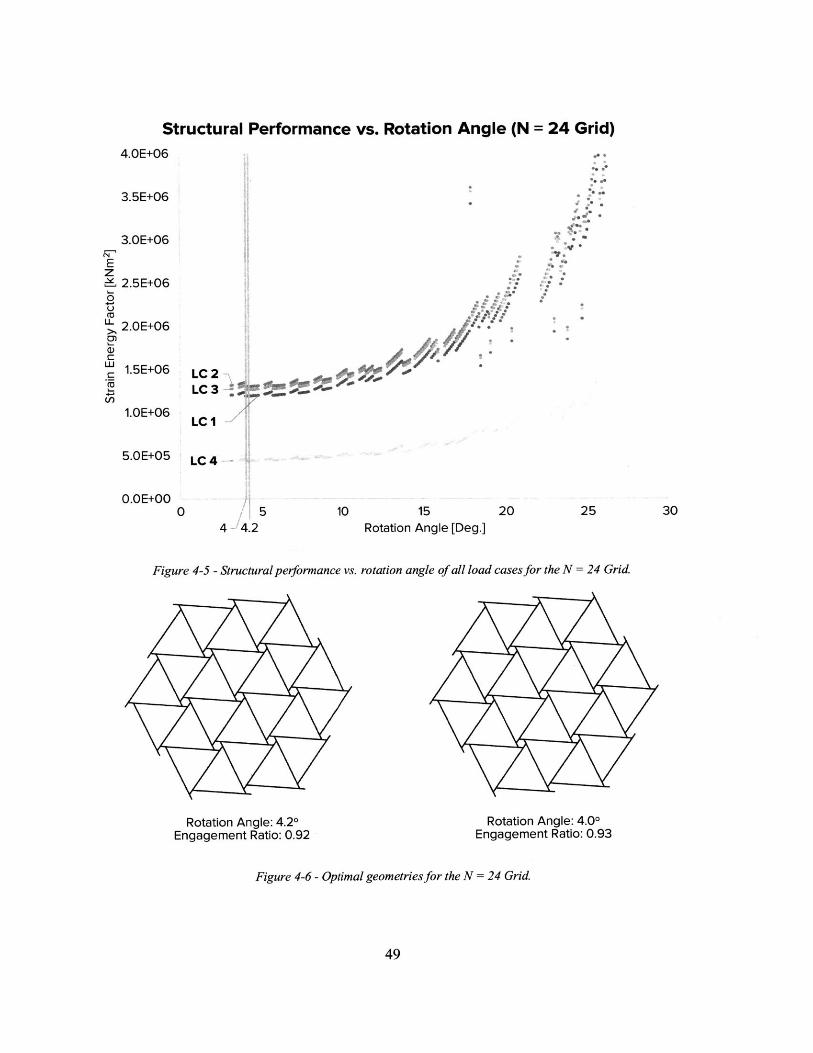
Structural Performance vs. Rotation Angle (N = 24 Grid)
4.0E+06
3.5E+06
3.0E+06
Ezi 2.5E+060U
u 2.0E+06)
L 1.5E+06
1.OE+06
5.0E+05
O.OE+00
4"
LC 2LC 3
LC I
LC 4
0 5 10 15 20 254 4.2 Rotation Angle [Deg.]
Figure 4-5 - Structural performance vs. rotation angle of all load cases for the N = 24 Grid.
Rotation Angle: 4.20Engagement Ratio: 0.92
Rotation Angle: 4.00Engagement Ratio: 0.93
Figure 4-6 - Optimal geometries for the N = 24 Grid.
49
30
4.4.1. Variation of Maximum Moments for N = 24 Grid
Figure 4-7 shows the value of maximum moments at each rotation angle for the seven member
types under symmetric loading (load case 1). Figure 4-8 shows the member type maximum
moments under the most asymmetric loading (load case 4).
Maximum Moments for LC 1 (N = 24 Grid)180
160
140
120
z
100E0
o)~ 80
C(D60
/-
Type 7Type 6
-~ ~ -~
Type 2
Type 1
15Rotation Angle [Deg.]
Figure 4-7 - LC I maximum moments for each member type in the N = 24 Grid.
50
Type 5
Type 3
40
20
0
Type 4
0 5
4.2
10 20 25 30
Maximum Moments for LC 4 (N = 24 Grid)120
100
Type 7 Type 6
-0
10 15Rotation Angle [Deg.]
Figure 4-8 - LC 4 maximum moments for each member type in the N
51
80Ez
Eo 60
40).C
m40Type 5
/
7.IType 4
Type 3
Type 2
Type I
20
00 4 5 20 25 30
24 Grid.
0-10-00001" .OOW
.0.0- OOOW
4.4.2. Discussion of Results for N = 24 Grid
Similar to the N = 6 Grid, the optimal rotation angle does not lie at an extremity but at 4.2 or 4.0
degrees. Although the optimal rotation angle for load case 4 is 0.2 degrees off from the other 3
load cases, the relative difference in the Strain Energy Factor for 4.2 and 4.0 degrees is only 0.06%
in load case 4, which can be considered negligible in terms of compromised efficiency. Note that
the Strain Energy Factor is relatively flat for low rotation angles up to about 7 degrees; this
correlates with the small difference in values between 4.2 and 4.0 degrees, and suggests that this
range of rotation angles all produce similarly efficient geometries.
Similar to the N = 6 grid results, the maximum moment and structural performance graphs
are closely correlated. However, the shapes of the graphs are dramatically different from the N =
6 grid: although a minimum is still found at a rotation angle that is not the smallest possible, the
values increase at a much more rapid rate as the rotation angle increases, in contrast with the N
6 grid where the values flatten out after about 19 degrees.
In terms of member type maximum moments, the trend is similar to the N = 6 grid in the
sense that an asymmetric loading case brings the moment values between members in closer
proximity. The member types also appear to be grouped according to their maximum moments:
types 1 and 2 are close to one another; types 3. 4 and 5 are close to one another; and types 6 and 7
are close to one another. This makes sense when we revisit Section 3.8 and note the relative
locations of the member types radially from the center. An interesting observation is the crossing
over of maximum moments between certain member types: for example, the maximum moment
of member type 3 crosses over member type 4 at about 12.5 degrees. Finally, in line with the
structural performance graph, the graph of maximum moments is relatively flat for member types
3 to 7 for low rotation angles.
52
4.5. N = 96 Grid Results
Key analysis outputs of the optimal rotation angle for the four load cases are tabulated in Table
4-3. The Strain Energy Factor for each rotation angle is plotted in Figure 4-9. The geometry at the
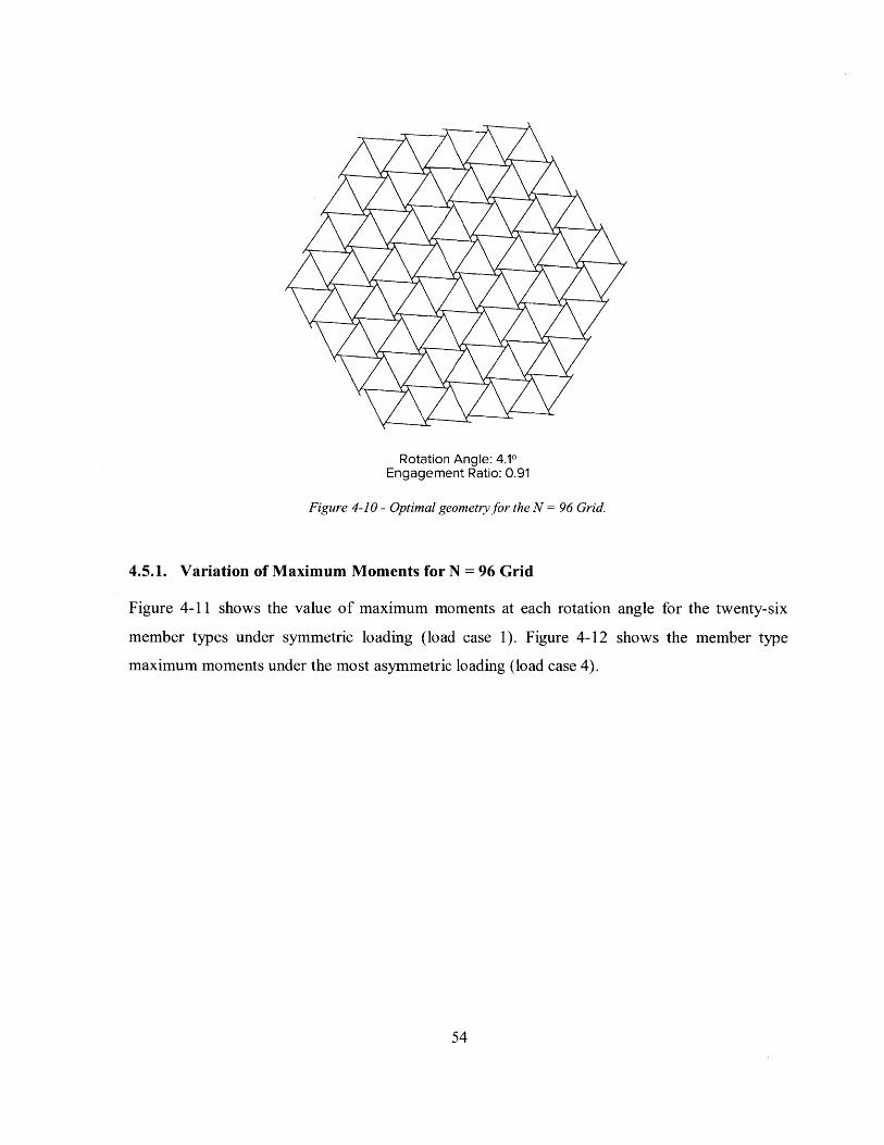
optimal angles of 4.1 degrees is shown in Figure 4-10.
At Optimal: LC 1 LC 2 LC 3 LC 4
Rotation Angle [Deg.] 4.1 4.1 4.1 4.1
EMmax 2 [kNm2 ] 6.32 x 10⁵ 6.82 x 10⁵ 6.73 x 10' 2.37 x 10'
Engagement Ratio 0.91 0.91 0.91 0.91
Maximum Moment [kNm] 28.5 31.9 29.4 19.6
Deflection Ratio L/248 L/207 L/240 L/414
Table 4-3 - Analysis outputs of the optimal angle for each load case in the N = 96 Grid.
Structural Performance vs. Rotation Angle (N = 96 Grid)1.4E+06
1.2E+06
N-1.0E+06
z
0 8.01E+05U
0)
W6.0E+05
C
(I)
.. ~
I./
LC 2
LC 3
LC 1
4.0E+05
LC 42.OE+05
0.0E+000 5 10 15 20
4.1 Rotation Angle [Deg.]
Figure 4-9 - Structural performance vs. rotation angle of all load cases br the N
25 30
96 Grid.
53
Rotation Angle: 4.10Engagement Ratio: 0.91
Figure 4-10 - Optimal geometry for the N = 96 Grid.
4.5.1. Variation of Maximum Moments for N = 96 Grid
Figure 4-11 shows the value of maximum moments at each rotation angle for the twenty-six
member types under symmetric loading (load case 1). Figure 4-12 shows the member type
maximum moments under the most asymmetric loading (load case 4).
54
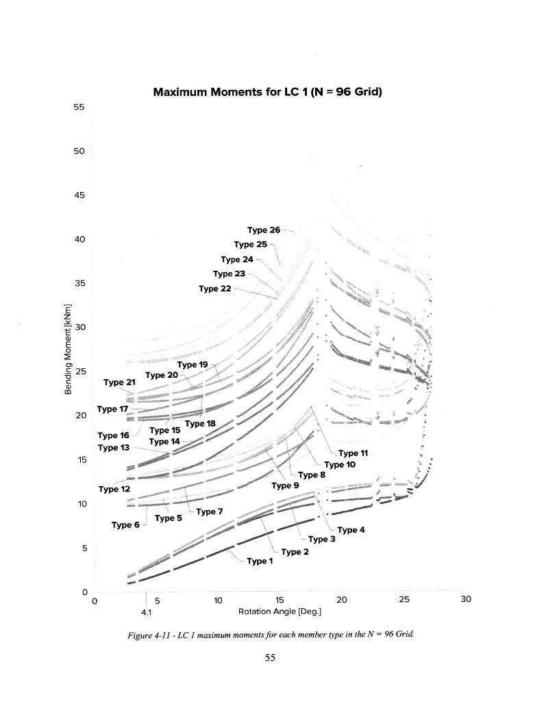
Maximum Moments for LC I (N = 96 Grid)55
50
45
Type 26
Type 25
Type 24
Type 23
Type 22
rype 2Type 19
Type 18Type 15T 4^y Flu
E~ -~-V
Type 5Type 7
5
Type 1
.S
- a
Ni'K
Vr*
Type 11Type 10
Type 8Type 9
~r
"'Vcz'r
rW Type 4Type 3
Type 2
- -a----
5 10 15 20 254.1 Rotation Angle [Deg.]
Figure 4-11 - LC 1 maximum moments for each member type in the N = 96 Grid.
55
40
35
z30
E0
0)E25
20
-IType 21
Type 17
Type 16
Type 13
15
Type 12
10
Type 6
00 30
IMaximum Moments for LC 4 (N = 96 Grid)
40
35
Type 25
Type 24
Type 26
Typ
25 Type 2
Type 20
Type 19Type 18
20 Type 17
Type 23
Type 15
15 Type 14Type 16 Type 13
Typel2 1
'-NA-
e21
2
41, 4
-
Type 11
Type 10
Type 8-
Type 9Type 7
Type 6
5
-I---
-a-----
-wo
Type 5Type 4
Type 2
Type 3Type 1
5 10 15 20 254.1 Rotation Angle [Deg.]
Figure 4-12 - LC 4 maximum momentsfor each member type in the N = 96 Grid.
56
30
Tz
E0
10
00 30
4.5.2. Discussion of Results for N = 96 Grid
Similar to the two previous grid densities, the optimal rotation angle does not occur at an extremity
but at 4.1 degrees, and in this case is the optimal for all load cases. In addition, the angle is very
similar to that of the N = 24 optimal (4.2 degrees).
As expected, the structural performance and maximum moment graphs generally correlate.
In addition, the graphs also appear to return to the likeliness of the N = 6 grid results: the Strain
Energy Factor increases up to around 19 degrees, then flattens out. For the maximum moments,
they increase up to 19 degrees, then decrease like the N = 6 grid. Furthermore, the curve of
maximum moments in the type 1-4 members closely resembles that of the type 1 members in the
N = 6 grid.
Finally, the maximum moments are also grouped in a similar manner like the N = 24 grid:
types I to 4 are one group, followed by types 5 to 7; types 8 to 11; types 12 to 14; types 15 to 17;
types 18 to 21; and types 22 to 26. The crossing over of maximum moments between member
types is also evident in this grid density.
Based on the results for all grid densities, it can be concluded that the most efficient
geometry for symmetric loading is also relatively efficient for asymmetric loading. The
implications of this result is positive as it suggests that for a given RF grid structure with any
particular geometry, it would not be performing in a greatly inefficient manner when subject to
asymmetric loading.
57
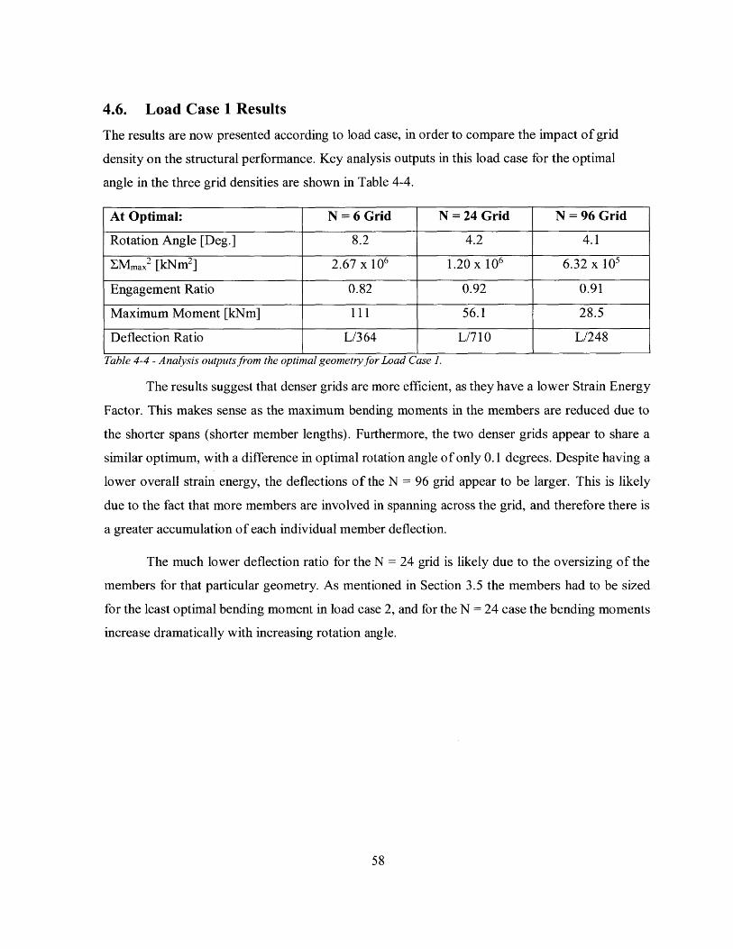
4.6. Load Case 1 Results
The results are now presented according to load case, in order to compare the impact of grid
density on the structural performance. Key analysis outputs in this load case for the optimal
angle in the three grid densities are shown in Table 4-4.
At Optimal: N = 6 Grid N = 24 Grid N = 96 Grid
Rotation Angle [Deg.] 8.2 4.2 4.1
EMmax 2 [kNm 2] 2.67 x 10⁶ 1.20 x 10⁶ 6.32 x 10'
Engagement Ratio 0.82 0.92 0.91
Maximum Moment [kNm] 111 56.1 28.5
Deflection Ratio L/364 L/710 L/248
Table 4-4 - Analysis outputs from the optimal geometry for Load Case 1.
The results suggest that denser grids are more efficient, as they have a lower Strain Energy
Factor. This makes sense as the maximum bending moments in the members are reduced due to
the shorter spans (shorter member lengths). Furthermore, the two denser grids appear to share a
similar optimum, with a difference in optimal rotation angle of only 0.1 degrees. Despite having a
lower overall strain energy, the deflections of the N = 96 grid appear to be larger. This is likely
due to the fact that more members are involved in spanning across the grid, and therefore there is
a greater accumulation of each individual member deflection.
The much lower deflection ratio for the N = 24 grid is likely due to the oversizing of the
members for that particular geometry. As mentioned in Section 3.5 the members had to be sized
for the least optimal bending moment in load case 2, and for the N = 24 case the bending moments
increase dramatically with increasing rotation angle.
58
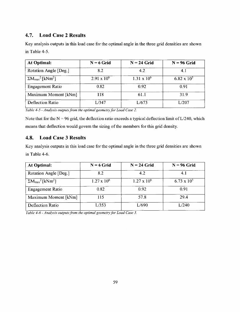
4.7. Load Case 2 Results
Key analysis outputs in this load case for the optimal angle in the three grid densities are shown
in Table 4-5.
At Optimal: N = 6 Grid N = 24 Grid N = 96 Grid
Rotation Angle [Deg.] 8.2 4.2 4.1
EMmax2 [kNm2] 2.91 x 10⁶ 1.31 x 10⁶ 6.82 x 10⁵
Engagement Ratio 0.82 0.92 0.91
Maximum Moment [kNm] 118 61.1 31.9
Deflection Ratio L/347 L/673 L/207
Table 4-5 - Analysis outputs from the optimal geometry for Load Case 2.
Note that for the N = 96 grid, the deflection ratio exceeds a typical deflection limit of L/240, which
means that deflection would govern the sizing of the members for this grid density.
4.8. Load Case 3 Results
Key analysis outputs in this load case for the optimal angle in the three grid densities are shown
in Table 4-6.
At Optimal: N = 6 Grid N = 24 Grid N = 96 Grid
Rotation Angle [Deg.] 8.2 4.2 4.1
IMmax 2 [kNm 2] 1.27 x 10⁶ 1.27 x 10⁶ 6.73 x 10⁵
Engagement Ratio 0.82 0.92 0.91
Maximum Moment [kNm] 115 57.8 29.4
Deflection Ratio L/353 L/690 L/240
Table 4-6 - Analysis outputs from the optimal geometry for Load Case 3.
59
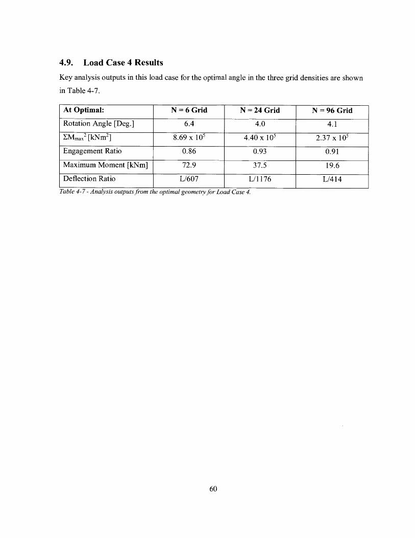
4.9. Load Case 4 Results
Key analysis outputs in this load case for the optimal angle in the three grid densities are shown
in Table 4-7.
At Optimal: N = 6 Grid N = 24 Grid N = 96 Grid
Rotation Angle [Deg.] 6.4 4.0 4.1
EMmax 2 [kNm 2] 8.69 x 10⁵ 4.40 x 10' 2.37 x 10'
Engagement Ratio 0.86 0.93 0.91
Maximum Moment [kNm] 72.9 37.5 19.6
Deflection Ratio L/607 L/ 176 L/414
Table 4-7 - Analysis outputs from the optimal geometry for Load Case 4.
60
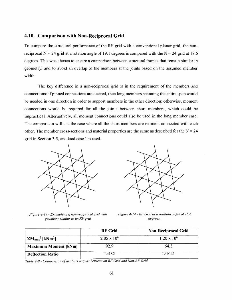
4.10. Comparison with Non-Reciprocal Grid
To compare the structural performance of the RF grid with a conventional planar grid, the non-
reciprocal N = 24 grid at a rotation angle of 19.1 degrees is compared with the N = 24 grid at 18.6
degrees. This was chosen to ensure a comparison between structural frames that remain similar in
geometry, and to avoid an overlap of the members at the joints based on the assumed member
width.
The key difference in a non-reciprocal grid is in the requirement of the members and
connections: if pinned connections are desired, then long members spanning the entire span would
be needed in one direction in order to support members in the other direction; otherwise, moment
connections would be required for all the joints between short members, which could be
impractical. Alternatively, all moment connections could also be used in the long member case.
The comparison will use the case where all the short members are moment connected with each
other. The member cross-sections and material properties are the same as described for the N = 24
grid in Section 3.5, and load case 1 is used.
Figure 4-13 - Example of a non-reciprocal grid withgeometry similar to an RF grid.
Figure 4-14 - RF Grid at a rotation angle of 18.6degrees.
RF Grid Non-Reciprocal Grid
EMmax2 [kNm 2 ] 2.05 x 10⁶ 1.20 x 10⁶
Maximum Moment [kNm] 92.9 64.3
Deflection Ratio L/482 L/1041
Table 4-8 - Comparison of analysis outputs between an RF Grid and Non-RF Grid.
61

The Strain Energy Factor for the non-reciprocal grid is lower than that of the RF grid,
which means that the non-reciprocal grid is more efficient according to our definition. This finding
correlates with the comparison performed by Gelez et al. (2011), between an RF grid of rectangular
topology and a conventional grid: the RF grid is not able to compete in terms of maximum bending
moment and deflection, and therefore has more total strain energy. However as noted in the
literature review, an RF grid remains advantageous in terms of robustness achieved through
redundancy, constructability through the use of shorter members and simple pin connections, and
adaptability to irregular perimeters.
62
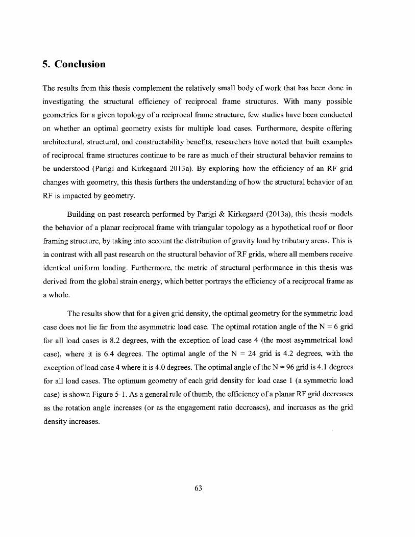
5. Conclusion
The results from this thesis complement the relatively small body of work that has been done in
investigating the structural efficiency of reciprocal frame structures. With many possible
geometries for a given topology of a reciprocal frame structure, few studies have been conducted
on whether an optimal geometry exists for multiple load cases. Furthermore, despite offering
architectural, structural, and constructability benefits, researchers have noted that built examples
of reciprocal frame structures continue to be rare as much of their structural behavior remains to
be understood (Parigi and Kirkegaard 2013a). By exploring how the efficiency of an RF grid
changes with geometry, this thesis furthers the understanding of how the structural behavior of an
RF is impacted by geometry.
Building on past research performed by Parigi & Kirkegaard (2013a), this thesis models
the behavior of a planar reciprocal frame with triangular topology as a hypothetical roof or floor
framing structure, by taking into account the distribution of gravity load by tributary areas. This is
in contrast with all past research on the structural behavior of RF grids, where all members receive
identical uniform loading. Furthermore, the metric of structural performance in this thesis was
derived from the global strain energy, which better portrays the efficiency of a reciprocal frame as
a whole.
The results show that for a given grid density, the optimal geometry for the symmetric load
case does not lie far from the asymmetric load case. The optimal rotation angle of the N = 6 grid
for all load cases is 8.2 degrees, with the exception of load case 4 (the most asymmetrical load
case), where it is 6.4 degrees. The optimal angle of the N = 24 grid is 4.2 degrees, with the
exception of load case 4 where it is 4.0 degrees. The optimal angle of the N = 96 grid is 4.1 degrees
for all load cases. The optimum geometry of each grid density for load case 1 (a symmetric load
case) is shown Figure 5-1. As a general rule of thumb, the efficiency of a planar RF grid decreases
as the rotation angle increases (or as the engagement ratio decreases), and increases as the grid
density increases.
63
N = 6 GridRotation Angle: 8.20
Engagement Ratio: 0.82
N = 24 GridRotation Angle: 4.20
Engagement Ratio: 0.92
N = 96 GridRotation Angle: 4.10
Engagement Ratio: 0.91
Figure 5-1 - Optimal geometries for load case 1.
The results are promising as they suggest that planar RF structures are a good fit for cases
where asymmetric loading may occur frequently, since their geometric configuration would not be
much less efficient than if it was loaded symmetrically. Given that asymmetric loading often
occurs for a floor or roof framing structure, the results suggest that a planar RF structure is a good
fit for that application.
C.i. i Uur Wory
Potential for future work includes expanding the research to additional RF topologies. For
topologies where the geometry cannot be described in terms of a rotation angle (for instance the
rectangular topology), the size of the engagement window can be used to compare results between
different topologies. It would be valuable to determine whether the structural performance of the
rectangular topology decreases as the engagement window becomes smaller, and whether the most
efficient geometry under symmetric loading would also be close to the efficient geometry for
asymmetrical loading.
Another area of interest for further development is in the optimization of members based
on their member type, as mentioned in Section 3.8. It would be interesting to evaluate the material
savings that can be realized if each member type was optimized for their expected maximum
loading under both symmetric and asymmetric load cases.
64
6. References
American Society of Civil Engineers. 2013. Minimum Design Loads for Buildings and OtherStructures. In ASCE 7-10. Reston, Virginia: American Society of Civil Engineers.
Baverel, 0. 2004. "Configuration Processing of Nexorades using Genetic Algorithms." Journalof the International Association for Shell and Spatial Structures 45:99-108.
European Committee for Standardization. 2003. Structural timber - Strength classes (EN 338).Gelez, Simon, Simon Aubry, and Bernard Vaudeville. 2011. "Behavior of a Simple Nexorade or
Reciprocal Frame System." International Journal of Space Structures 26 (4):331-342.Kaethner, S.C., and J.A. Burridge. 2012. "Embodied C02 of structural frames." The Structural
Engineer 90 (5):33-40.Kingsford, Ed. KREOD / Chun Qing Li of Pavilion Architecture.Kirkegaard, Poul Henning, and Dario Parigi. 2013b. "Robustness Analysis of Typologies of
Reciprocal Timber Structures." International Association for Shell and Spatial StructuresSymposium, Poland.
Kohlhammer, Thomas, and Toni Kotnik. 2011. "Systemic Behaviour of Plane Reciprocal FrameStructures." Structural Engineering International 21 (1):80-86. doi:10.2749/10168661 1x12910257102596.
Larsen, 0. P. 2014. "Reciprocal Frame (RF) Structures: Real and Exploratory." Nexus NetworkJournal 16 (1):119-134. doi: 10.1007/s00004-014-0181-0.
Larsen, Olga Popovic. 2008. Reciprocal Frame Architecture. Oxford, UK: Elsevier.Larsen, Olga Popovic, and Daniel Sang-Hoon Lee. 2013. "Reciprocal Frames (RFs) Used for
Quick-built Deployable Emergency Shelters." International Association for Shell andSpatial Structures (IASS) Symposium, Poland.
Microsoft Excel 2016. Microsoft.Parigi, Dario, and Poul Henning Kirkegaard. 2013a. "Structural Behaviour of Reciprocal
Structures." International Association for Shell and Spatial Structures (IASS) Symposium,Poland.
Preisinger, Clemens. Karamba 1.1.0.Robert McNeel & Associates. GhPython 0.6.0.3.Robert McNeel & Associates. Grasshopper 0.9.0076.Robert McNeel & Associates. Rhinoceros Version 5 SR12.
65

66
Appendix A
This appendix contains the spreadsheet of the hand calculation verification discussed in Section
3.9. The equations used to solve for the unknown forces shaded in light grey are found in Section
3.9. The shear force at a node is calculated from summing the shear force at the previous node
with the applied force on the node. "dM" represents the change in bending moment between two
nodes, which is calculated from the area of the shear diagram between two nodes. The value of
moment at a given node is therefore the sum of the moment at the previous node and the change
in moment (dM).
67
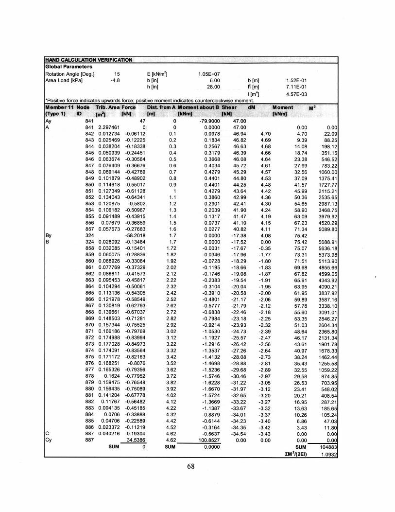
HAND CALCULATION VERIFICATIONGlobal ParametersRotation Angle [Deg.] 15 E [kN/m2 ] 1.05E+07Area Load [kPa] -4.8 b [in] 6.00 b [m] 1.52E-01
h [in] 28.00 hi [m] 7.11E-011 [M4
] 4.57E-03*Positive force indicates upwards force; positive moment indicates counterclockwise moment.
Node Trib. Area ForceID [M 2] [kN]
Member 11(Type 1)AyA
ByB
CCy
841841842843844845846847848849850851852853854855856857324324858859860861862863864865866867868869870871872873874875876877878879880881882883884885886887887
Shear[kNI
dM
2.2974610.0127340.0254690.0382040.0509390.0636740.0764090.0891440.1018790.1146180.1273490.1340430.1208750.1061820.0914890.07679
0.057673
0.0280920.0320850.0600750.0689260.0777690.0866110.0954530.1042940.1131360.1219780.1308190.1396610.1485030.1573440.1661860.1749880.1770280.1740910.1711720.1682510.165326
0.16240.1594750.1564350.141204
0.117670.094135
0.07060.04706
0.0233720.040216
Moment[kNm]
470
-0.06112-0.12225-0.18338-0.24451-0.30564-0.36676-0.42789-0.48902-0.55017-0.61128-0.64341-0.5802
-0.50967-0.43915-0.36859-0.27683-58.2018-0.13484-0.15401-0.28836-0.33084-0.37329-0.41573-0.45817-0.50061-0.54305-0.58549-0.62793-0.67037-0.71281-0.75525-0.79769-0.83994-0.84973-0.83564-0.82163-0.8076
-0.79356-0.77952-0.76548-0.75089-0.67778-0.56482-0.45185-0.33888-0.22589-0.11219-0.1930434.5386
0
Dist. from A[im]
00
0.10.20.30.40.50.60.70.80.9
11.11.21.31.41.51.61.71.7
1.721.821.922.022.122.222.322.422.522.622.722.822.923.023.123.223.323.423.523.623.723.823.924.024.124.224.324.424.524.62
Moment about B[kNm]
-79.90000.00000.09780.18340.25670.31790.36680.40340.42790.44010.44010.42790.38600.29010.20390.13170.07370.02770.00000.0000
-0.0031-0.0346-0.0728-0.1195-0.1746-0.2383-0.3104-0.3910-0.4801-0.5777-0.6838-0.7984-0.9214-1.0530-1.1927-1.2916-1.3537-1 .4132-1.4698-1.5236-1.5746-1.6228-1.6670-1.5724-1.3669-1.1387-0.8879-0.6144-0.3164-0.5637
68
47.0047.0046.9446.8246.6346.3946.0845.7245.2944.8044.2543.6442.9942.4141.9041.4741.1040.82
-17.38-17.52-17.67-17.96-18.29-18.66-19.08-19.54-20.04-20.58-21.17-21.79-22.46-23.18-23.93-24.73-25.57-26.42-27.26-28.08-28.88-29.68-30.46-31.22-31.97-32.65-33.22-33.67-34.01-34.23-34.35-34.54
0.00
4.704.694.684.664.644.614.574.534.484.424.364.304.244.194.154.114.080.00
-0.35-1.77-1.80-1.83-1.87-1.91-1.95-2.00-2.06-2.12-2.18-2.25-2.32-2.39-2.47-2.56-2.64-2.73-2.81-2.89-2.97-3.05-3.12-3.20-3.27-3.32-3.37-3.40-3.42-3.430.004.62 100.8527
SUM 0.0000
0.004.709.39
14.0818.7423.3827.9932.5637.0941.5745.9950.3654.6558.9063.0967.2371.3475.4275.4275.0773.3171.5169.6867.8265.9163.9561.9559.8957.7855.6053.3551.0348.6446.1743.6140.9738.2435.4332.5529.5826.5323.4120.2116.9513.6310.266.863.430.000.00
SUMEM 2/(2EI)
0.0022.0988.25
198.12351.15546.52783.22
1060.001375.411727.772115.212535.652987.133468.753979.924520.295089.80
5688.915636.185373.985113.904855.664599.054343.924090.213837.923587.163338.103091.012846.272604.342365.802131.341901.781678.331462.441255.581059.22874.85703.95548.02408.54287.21185.65105.2447.0311.800.000.00
1048831.0932
SUM
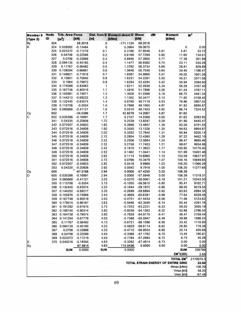
Member 0(Type 2)ByB
CyC
DyD
EEy
Dist. from B[m]
Node Trib. Area ForceID [m 2] [kN]
324 58.2018324 0.028092 -0.13484325 0.023372 -0.11219326 0.04706 -0.22589327 0.0706 -0.33888328 0.094135 -0.45185329 0.11767 -0.56482330 0.139294 -0.66861331 0.149621 -0.71818332 0.15801 -0.75845333 0.1664 -0.79872334 0.174089 -0.83563335 0.167748 -0.80519336 0.155981 -0.74871337 0.144213 -0.69222338 0.132445 -0.63574339 0.115708 -0.5554340 0.085668 -0.41121652 -34.5386652 0.035398 -0.16991341 0.04335 -0.20808342 0.072507 -0.34803343 0.072516 -0.34808344 0.072518 -0.34809345 0.072518 -0.34809346 0.072518 -0.34809347 0.072518 -0.34809348 0.072518 -0.34809349 0.072518 -0.34809350 0.072518 -0.34809351 0.072516 -0.34808352 0.072507 -0.34803353 0.04335 -0.20808605 -67.2168605 0.035398 -0.16991354 0.085668 -0.41121355 0.115708 -0.5554356 0.132445 -0.63574357 0.144202 -0.69217358 0.155976 -0.74868359 0.167748 -0.80519360 0.179515 -0.86167361 0.191282 -0.91815362 0.188155 -0.90314363 0.164738 -0.79074364 0.141204 -0.67778365 0.11767 -0.56482366 0.094135 -0.45185367 0.0706 -0.33888368 0.04706 -0.22589369 0.023372 -0.11219370 0.040216 -0.19304
67.4814SUM 0.0000
[kNm]00
0.10.20.30.40.50.60.70.80.9
11.11.21.31.41.51.61.71.7
1.721.821.922.022.122.222.322.422.522.622.722.822.922.942.943.033.133.233.333.433.533.633.733.833.934.034.134.234.334.434.534.634.63 114.0436
SUM 0.0000
TOTAL yM2 2170074.3
TOTAL STRAIN ENERGY OF ENTIRE GRID 22.62Mmax [kNm] 106.39
Vmax [kN] 58.20Vmin [kN] -67.48
69
M ome nt about D Shear dM[kN]
Moment[kNm]
I-171.1134
0.39640.31860.61890.89461.14771.37821.56461.60871.62311.62941.62111.48161.30281.13520.97900.79980.5510
42.82790.21070.25390.38980.35500.32020.28540.25060.21580.18100.14620.11140.07660.04180.00420.00000.0000-0.0370-0.1055-0.1844-0.2699-0.3669-0.4751-0.5946-0.7253-0.8038-0.7828-0.7388-0.6721-0.5829-0.4710-0.3366-0.1784-0.3262
58.201858.067057.954857.728957.390056.938256.373455.704854.986654.228153.429452.593851.788651.039950.347749.711949.156548.745314.206714.036813.828713.480713.132612.784512.436512.088411.740311.392211.044110.696010.34799.99999.7918
-57.4250-57.5949-58.0061-58.5615-59.1972-59.8894-60.6381-61.4433-62.3049-63.2231-64.1262-64.9170-65.5947-66.1596-66.6114-66.9503-67.1762-67.2884-67.4814
0.0000
5.815.805.775.745.695.645.575.505.425.345.265.185.105.034.974.924.870.000.281.381.351.311.281.241.211.171.141.101.071.031.000.200.00
-5.18-5.80-5.86-5.92-5.99-6.06-6.14-6.23-6.32-6.41-6.49-6.56-6.62-6.66-6.70-6.72-6.730.00
05.81
11.6017.3823.1128.8134.4540.0245.5150.9456.2861.5466.7271.8276.8681.8386.7491.6291.6291.9093.2894.6395.9497.2298.4799.67
100.85101.99103.09104.16105.20106.20106.39106.39101.2195.4189.5583.6377.6471.5865.4459.2052.8846.4739.9833.4226.8020.1413.456.730.000.00
SUMEM 2/(2EI)
0.0033.72
134.61301.89534.26829.89
1186.471601.262071.562594.603167.453787.114451.345158.455907.026695.877524.52
8393.958445.478701.558954.879205.149452.109695.469934.98
10170.4010401.4810627.9710849.6511066.2911277.68
11319.3110243.209102.718019.556994.356028.485123.624281.763505.192796.552159.441598.241116.80718.38405.68180.8145.28
0.000.00
2567962.68