1

George Philippidis Ana I. Sanjuán Emanuele Ferrari Robert M'barek

Structural Patterns of the Bioeconomy in the

EU Member States – a SAM approach

2014

Report EUR 26773

2

European Commission

Joint Research Centre

Institute for Prospective Technological Studies

Contact information

Address: Joint Research Centre, Edificio EXPO, Calle Inca Garcilaso, 3, 41092, Seville, Spain

E-mail: jrc-ipts-agrilife-secretariat@ec.europa.eu

Tel.: +34 954 4884348

https://ec.europa.eu/jrc

https://ec.europa.eu/jrc/en/institutes/ipts

Legal Notice

This publication is a Science and Policy Report by the Joint Research Centre, the European Commission’s in-house science

service. It aims to provide evidence-based scientific support to the European policy-making process. The scientific output

expressed does not imply a policy position of the European Commission. Neither the European Commission nor any person

acting on behalf of the Commission is responsible for the use which might be made of this publication.

All images © European Union 2014, except cover pictures, top: © badmanproduction - Fotolia , second line from left to

right: © Željko Radojko – Fotolia, © intheskies – Fotolia, © Gina Sanders - Fotolia

JRC90698

EUR 26773

ISBN 978-92-79-39530-7 (PDF)

ISSN 1831-9424 (online)

doi:10.2791/10584

Luxembourg: Publications Office of the European Union, 2014

© European Union, 2014

Reproduction is authorised provided the source is acknowledged.

Abstract

The concept of 'bioeconomy' is gathering momentum in European Union (EU) policy circles as a sustainable model of

growth to reconcile the goals of continued wealth generation and employment with bio-based sustainable resource usage.

Unfortunately, an economy-wide quantitative assessment covering the full diversity of this sector is, hitherto, constrained

by relatively poor data availability for disaggregated bio-based activities. This research takes a first step in addressing this

issue by employing social accounting matrices (SAMs) for each EU27 member encompassing a highly disaggregated

treatment of traditional bio-based agricultural and food sectors, in addition to identifiable bioeconomic activities from the

national accounts data. Employing backward-linkage (BL), forward-linkage (FL) and employment multipliers, the aim is to

profile and assess comparative structural patterns both across bioeconomic sectors and EU Member States. The results

indicate six clusters of EU member countries with homogeneous bioeconomy structures. Within cluster statistical tests

reveal a high tendency toward 'backward orientation' or demand driven wealth generation, whilst inter-cluster statistical

comparisons across each bio-based sector show only a moderate degree of heterogeneous BL wealth generation and, with

the exception of only two sectors, a uniformly homogeneous degree of FL wealth generation. With the exception of

forestry, fishing and wood activities, bio-based employment generation prospects are below non bioeconomy activities.

Finally, milk and dairy are established as 'key sectors'.

1

Table of Contents

1. Introduction ................................................................................................................................................ 2

2. Materials and Methods ............................................................................................................................ 6

2.1 SAMs and Multipliers ........................................................................................................................ 6

2.2 AgroSAM Database and Update to 2007 ................................................................................... 7

3. Results ......................................................................................................................................................... 10

3.1 Statistical Profiling of the EU Regional Clusters. ................................................................. 10

3.2. Statistical Profiling of Bioeconomy Sector Multipliers ..................................................... 13

3.3. Bioeconomy Employment Multipliers .................................................................................... 18

3.4. Key Sector Analysis ........................................................................................................................ 20

4. Conclusions ................................................................................................................................................ 26

References ...................................................................................................................................................... 29

2

1. Introduction In the 21

st century, the issues of climate change, natural resource depletion, population

growth and environmental degradation, to name but a few, are posing challenging questions

for policy makers. As a significant political and economic player on the world stage, the

European Union (EU) has taken a pro-active role in areas relating to greenhouse gas (GHG)

emissions reductions, renewable energy usage and the greening of its agricultural policy.

More recently, in 2012, a policy strategy paper (EC, 2012, p.3) was released by the European

Commission (EC) for a sustainable model of growth which could reconcile the goals of

continued wealth generation and employment with sustainable resource usage. To this end,

the term 'bioeconomy' was coined which, "encompasses the production of renewable

biological resources and the conversion of these resources and waste streams into value

added products, such as food, feed, bio-based products and bioenergy" (EC, 2012, p.3).

Under this definition, one is led to understand that bio-based output not only includes more

obvious examples such as agricultural and food output, but can be extended to embrace any

additional value added activities which employ organic matter of biological origin (i.e., non-

fossil) which is available on a renewable basis (e.g. plants, wood, residues, animal and

municipal wastes, fibres etc.).

The EU's Bioeconomy Strategy (EC, 2012) is an attempt to stimulate research and

development activities which can identify and enhance knowledge of bio-economic markets

and develop forward-looking policy recommendations to meet the aforementioned, and

sometimes conflicting, challenges.1

As an initial step to understanding the economic

importance of the bioeconomy in the EU, one must first have a clear picture of the status quo

relating to (inter alia) biomass' availability, potential bio-economic output and trade.

Unfortunately, questions of this nature give rise to immediate concerns regarding data

availability. For example, according to official estimates (EC, 2012) the EU bioeconomy

represents a market worth over EUR 2 trillion, providing 20 million jobs and accounting for

9% of total employment. Notwithstanding, these estimates remain imprecise since there is a

paucity of EU-wide comprehensive biomass balance sheets for varying uses (i.e., trade, fuel,

1 Indeed, encouraging biomass usage for energy may adversely affect carbon sequestration and therefore GHG

emissions limits. Similarly, implementing a strategy for responsible sustainable growth may induce limits on

employment generation in times of post-crisis.

3

waste uses etc.) (M'barek et al., 2014).2

Furthermore, existing national accounts data,

reported by Eurostat (2014a), has a very limited coverage of bioeconomic activities.

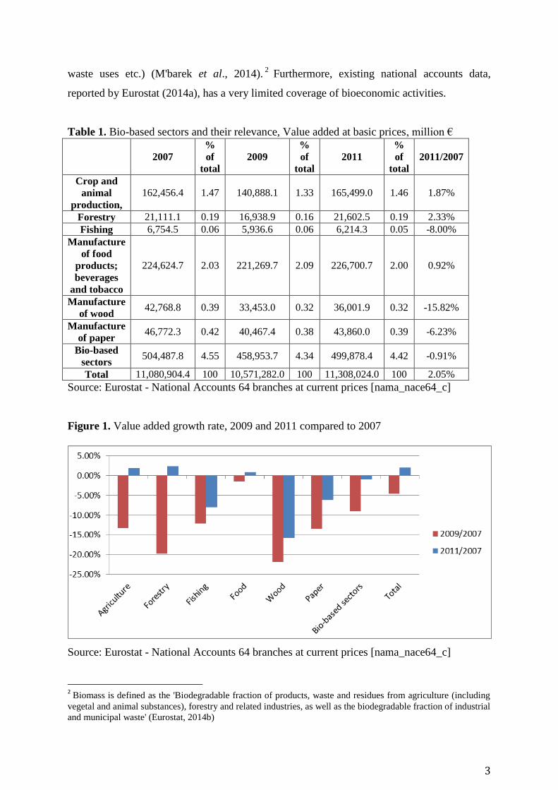
Table 1. Bio-based sectors and their relevance, Value added at basic prices, million €

2007

%

of

total

2009

%

of

total

2011

%

of

total

2011/2007

Crop and

animal

production,

162,456.4 1.47 140,888.1 1.33 165,499.0 1.46 1.87%

Forestry 21,111.1 0.19 16,938.9 0.16 21,602.5 0.19 2.33%

Fishing 6,754.5 0.06 5,936.6 0.06 6,214.3 0.05 -8.00%

Manufacture

of food

products;

beverages

and tobacco

224,624.7 2.03 221,269.7 2.09 226,700.7 2.00 0.92%

Manufacture

of wood 42,768.8 0.39 33,453.0 0.32 36,001.9 0.32 -15.82%

Manufacture

of paper 46,772.3 0.42 40,467.4 0.38 43,860.0 0.39 -6.23%

Bio-based

sectors 504,487.8 4.55 458,953.7 4.34 499,878.4 4.42 -0.91%

Total 11,080,904.4 100 10,571,282.0 100 11,308,024.0 100 2.05%

Source: Eurostat - National Accounts 64 branches at current prices [nama_nace64_c]

Figure 1. Value added growth rate, 2009 and 2011 compared to 2007

Source: Eurostat - National Accounts 64 branches at current prices [nama_nace64_c]

2 Biomass is defined as the 'Biodegradable fraction of products, waste and residues from agriculture (including

vegetal and animal substances), forestry and related industries, as well as the biodegradable fraction of industrial

and municipal waste' (Eurostat, 2014b)

4

As a (partial) response to this data limitation, the current study employs a complete set

of EU Member State social accounting matrices (SAMs) containing an unparalleled level of

sector disaggregation of the traditional bio-based agricultural and food sectors.3 Employing

an updated version of this data, the aim is to profile and assess comparative structural

patterns within 'identifiable' bioeconomic sectors across EU Member States. In particular, the

analysis also sets out to recognize those bioeconomic sectors which potentially maximise

economic value added, with a view to formulating a coherent approach for reconciling

wealth- and/or employment generation with sustainable resource usage.

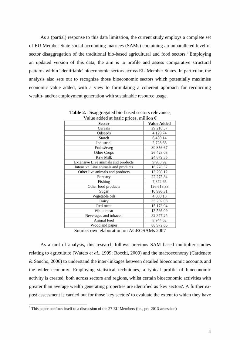
Table 2. Disaggregated bio-based sectors relevance,

Value added at basic prices, million € Sector Value Added

Cereals 29,210.57

Oilseeds 4,129.74

Starch 8,430.14

Industrial 2,728.68

Fruits&veg 39,356.67

Other Crops 26,428.03

Raw Milk 24,879.35

Extensive Live animals and products 9,903.92

Intensive Live animals and products 16,778.57

Other live animals and products 13,298.12

Forestry 22,275.84

Fishing 7,872.65

Other food products 126,618.33

Sugar 10,996.31

Vegetable oils 4,800.18

Dairy 35,202.08

Red meat 15,173.94

White meat 13,536.09

Beverages and tobacco 32,377.25

Animal feed 8,944.62

Wood and paper 88,972.65

Source: own elaboration on AGROSAMs 2007

As a tool of analysis, this research follows previous SAM based multiplier studies

relating to agriculture (Waters et al., 1999; Rocchi, 2009) and the macroeconomy (Cardenete

& Sancho, 2006) to understand the inter-linkages between detailed bioeconomic accounts and

the wider economy. Employing statistical techniques, a typical profile of bioeconomic

activity is created, both across sectors and regions, whilst certain bioeconomic activities with

greater than average wealth generating properties are identified as 'key sectors'. A further ex-

post assessment is carried out for those 'key sectors' to evaluate the extent to which they have

3 This paper confines itself to a discussion of the 27 EU Members (i.e., pre-2013 accession)

5

thrived in the ensuing period. The rest of this paper is organized as follows. Section 2

describes the methodology and database. Section 3 presents the results of the combined

multiplier and statistical analysis. Section 4 discusses main results and conclusions.

6

2. Materials and Methods

2.1 SAMs and Multipliers

The main theoretical developments in social accounting owe much to the work of Stone

(1955) by integrating the production accounts (in the form of input-output tables) into the

national accounts to create an economy-wide database. The resulting SAM database is a

square matrix which, for a given time period, provides a comprehensive, complete and

consistent picture of all economic transactions between productive and non-productive

institutions and markets, such as factor markets, savings-investments, households,

government, and the rest of the world. Thus, each cell entry simultaneously depicts an

expenditure flow from column account 'j' and an income flow to row account 'i', whilst

corresponding column and row account totals (i=j) must be equal (i.e., total expenditure

equals total income).

Due to its accounting consistency, comprehensiveness in recording data and flexibility,

the SAM approach (fix price linear models) in the last three decades has been extensively

used to analyse (inter alia) growth strategies in developing economies (Robinson, 1989),

income distribution and redistribution (Roland-Holst & Sancho, 1992), the circular flow of

income (Pyatt & Round, 1979; Defourny & Thorbecke 1984; Robinson and Roland- Holst

1988), price formation (Roland-Holst & Sancho, 1995), structural and policy analysis of the

agricultural sector in developed (Rocchi, 2009) and developing countries (Arndt et al., 2000),

and the effects of public policy on poverty reduction (De Miguel-Velez & Perez-Mayo,

2010).

Within a SAM model, all (endogenous4) accounts can be ranked according to a

hierarchy derived from two 'traditional' types of multiplier indices, known as the backward

linkage (BL) and a forward linkage (FL), calculated from the Leontief inverse (Rasmussen,

1956).5 Both FL and BL are 'relative' measures of supplier-buyer relationships within the

economy under conditions of Leontief (fixed-price) technologies. More specifically, for each

activity, the FL follows the distribution chain of bioeconomic outputs to end users, whilst the

BL examines upstream inter-linkages with intermediate input suppliers. Thus, for a given

sector, a BL or FL exceeding one implies that 1€ of intermediate input demand (BL) or

4 The endogenous accounts are those for which changes in expenditure directly follow any change in income,

while exogenous accounts are those for which expenditures are set independently of income. In SAM models,

Government and Rest of the World are typically held as exogenous. 5 As a substitute to the 'traditional' multiplier approach, the 'hypothetical extraction' model approach has also

been employed (e.g. Schultz, 1977; Dietzenbacher & van der Linden, 1997) to assess the importance of a sector

by analysing the impacts from its elimination.

7

supply (FL) generates a greater than average level (i.e., greater than €1) of wealth compared

with the remaining sectors of the economy. A sector with backward (forward) linkages

greater than one, and forward (backward) linkages less than one, is classified as backward

(forward) orientated. If neither linkage is greater than one, the sector is designated as 'weak',

whilst 'key sectors' are those which exhibit FL and BL values greater than one.

As a further tool of analysis, employment multipliers are calculated to examine the

generation of labour resulting from additional bioeconomic activity. More specifically, the

employment multiplier calculates the resulting 'direct', 'indirect' and 'induced' ripple effects

resulting from an increase or decrease in output value in activity ‘j’. Thus, the direct

employment effect is related to the output increase in the specific activity ‘j’, the indirect

employment effect is the result of a higher level of supporting industry activity, whilst the

induced employment effect is due to the change in household labour income demand for

sector ‘j’.6

2.2 AgroSAM Database and Update to 2007

An important obstacle to using a SAM based analysis for analysing the bioeconomy is

the high degree of sector aggregation typically found in the national accounts data. As the

main data source for constructing the SAM accounts, EU member state Supply- and Use-

Tables (SUT) traditionally represent bioeconomic activities as broad aggregates (i.e.,

agriculture, food processing, forestry, fishing, wood, pulp) or even subsume said activities

within their parent industries (e.g. chemical sector, wearing apparel, energy). Consequently,

this limits the scope of any study attempting to perform a detailed analysis of the

bioeconomy; whether it is SAM based (multipliers) or employing a computable general

equilibrium (CGE) framework.

As a (partial) response, a set of SAMs for each EU Member State, dubbed the

'AgroSAMs', was developed by the Joint Research Centre (JRC) of the EC benchmarked to

the year 2000 (Müller et al., 2009).7 This data source is the only EU-wide SAM based dataset

of its type, whilst a further important characteristic is the potential analytical insight resulting

from the unparalleled level of sector disaggregation of the bio-based agricultural and food

sectors (28 and 11 accounts, respectively). The construction of the AgroSAMs involved three

main steps (Müller et al., 2009): consolidating macroeconomic indicators for the EU27;

combining Eurostat datasets into a set of SAMs with aggregated agricultural and food-

6 See the appendix for a technical description of the multipliers used in this analysis.

7 In the latest two versions of the GTAP database (version 7 and 8), this dataset has been employed to populate

the I-O tables of the 27 EU member countries in the GTAP database.

8

industry accounts and finally; the disaggregation of agri-food accounts employing the

Common Agricultural Policy Regionalised Impacts analysis modelling system (CAPRI)

database (Britz & Witzke, 2012).

With the exception of the agriculture and food accounts, the AgroSAM follows the

same sectoral concordance as the Eurostat SUTs. Thus, of the 98 activity/commodity

accounts (see Table A.1 in the Appendix), 29 cover primary agriculture, one agricultural

services sector, 7 primary sectors (forestry, fishing and mining activities), 12 food

processing, 20 (non-food) manufacturing and construction, and 29 services sectors. In

addition, the AgroSAM contains two production factors (capital and labour), trade and

transportation margins and several tax accounts (taxes and subsidies on production and

consumption, VAT, import tariffs, direct taxes).8 Finally, there is a single account for the

private household, corporate activities, central government, investments-savings and the rest

of the world.

Although the AgroSAM provides a detailed disaggregation of agriculture and food

related bio-economic activities, the benchmark year of 2000 was no longer considered to be

relevant for meaningful policy analysis. Consequently, it was deemed necessary to perform

an update procedure prior to carrying out any subsequent multiplier analysis. A reasonably

proximate year of 2007 was selected based on the availability of Eurostat SUT information

for all EU Member States. Apart from the potential structural bias that may arise when

updating over long time periods, it was also not deemed wise to choose a 'crisis' period (i.e.,

post 2007) since the resulting shock to the economic system may have accelerated structural

change even further.9

As an initial step, all non agro-food productive rows and column cell entries are

overwritten with external data from the 2007 EU27 SUT tables (i.e., structure of industry

costs, commodity supplies, exports, imports, household- corporation- and government-final

demands, gross fixed capital formation, stock changes, margins and net taxes on production

and products). In a second step, the resulting SAM was inputted into a modified version of

the SAMBAL program for square matrices (Horridge, 2003). Aside from maintaining the

corresponding row and column balances, the SAMBAL program is further modified with

additional code to (i) target aggregate agricultural and food column totals to 2007; (ii)

8

The direct tax accounts include "Property income", "Current taxes on income and wealth", "Social

contributions and benefits", "Other current transfers" and "Adjustment for the change in net equity of

households in pension funds reserves" 9 In those cells where update assumptions are applied, it is recognised that the temporal gap should not be

excessive in order the limit structural change bias in the resulting updated SAM arising from technological

change in the ensuing period.

9

maintain 2007 Eurostat SUT non agri-food target totals as close as possible, and (iii) preserve

the economic structure of the SAM.

To achieve this, exogenous multiplier variables in each equation are swapped with

target variables. Furthermore, the update procedure also incorporates a set of behavioural

equations for certain flow values with a view to maintaining, as much as possible, the

structural integrity of the SAM, thereby avoiding large fluctuations in cell values when the

balancing procedure is carried out. For example, at the margin, taxes, subsidies and

retail/transport margins are assumed to change proportionally with the transactions upon

which they are levied. Moreover, given the difficulty of finding detailed institutional

accounts data for all of the EU27 members, it is assumed in the pre-crisis period (2000 to

2007) that cell entries vary in proportion to GDP.

For the agricultural industry accounts, the technical coefficients in the existing

AgroSAM were maintained subject to 2007 target data for value added and intermediate cost

totals taken from the Eurostat's 'economic accounts for agriculture' (Eurostat 2014a). This

data source was also employed to implement subsidies on production and products for the 28

agricultural accounts. Target values for agricultural and food exports and imports in 2007

were calculated employing the COMEXT database (Eurostat, 2014a), where a concordance

was carried out between the agricultural and food sectors in the AgroSAM and the Eurostat

HS2-HS4 sectors, supplemented by a HS6 concordance where necessary. To maintain the

macro restriction equating GDP by income and expenditure, data for 2007 on aggregate

demand by components are also taken from Eurostat (2014a).

10

3. Results

3.1 Statistical Profiling of the EU Regional Clusters.

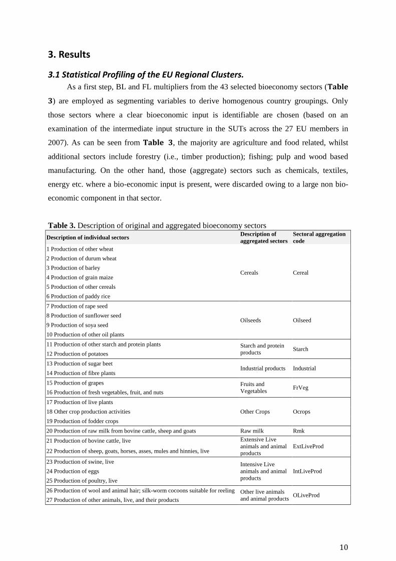
As a first step, BL and FL multipliers from the 43 selected bioeconomy sectors (Table

3) are employed as segmenting variables to derive homogenous country groupings. Only

those sectors where a clear bioeconomic input is identifiable are chosen (based on an

examination of the intermediate input structure in the SUTs across the 27 EU members in

2007). As can be seen from Table 3, the majority are agriculture and food related, whilst

additional sectors include forestry (i.e., timber production); fishing; pulp and wood based

manufacturing. On the other hand, those (aggregate) sectors such as chemicals, textiles,

energy etc. where a bio-economic input is present, were discarded owing to a large non bio-

economic component in that sector.

Table 3. Description of original and aggregated bioeconomy sectors

Description of individual sectors Description of

aggregated sectors

Sectoral aggregation

code

1 Production of other wheat

Cereals Cereal

2 Production of durum wheat

3 Production of barley

4 Production of grain maize

5 Production of other cereals

6 Production of paddy rice

7 Production of rape seed

Oilseeds Oilseed 8 Production of sunflower seed

9 Production of soya seed

10 Production of other oil plants

11 Production of other starch and protein plants Starch and protein

products Starch

12 Production of potatoes

13 Production of sugar beet Industrial products Industrial

14 Production of fibre plants

15 Production of grapes Fruits and

Vegetables FrVeg

16 Production of fresh vegetables, fruit, and nuts

17 Production of live plants

Other Crops Ocrops 18 Other crop production activities

19 Production of fodder crops

20 Production of raw milk from bovine cattle, sheep and goats Raw milk Rmk

21 Production of bovine cattle, live Extensive Live

animals and animal

products

ExtLiveProd 22 Production of sheep, goats, horses, asses, mules and hinnies, live

23 Production of swine, live Intensive Live

animals and animal

products

IntLiveProd 24 Production of eggs

25 Production of poultry, live

26 Production of wool and animal hair; silk-worm cocoons suitable for reeling Other live animals

and animal products OLiveProd

27 Production of other animals, live, and their products

11

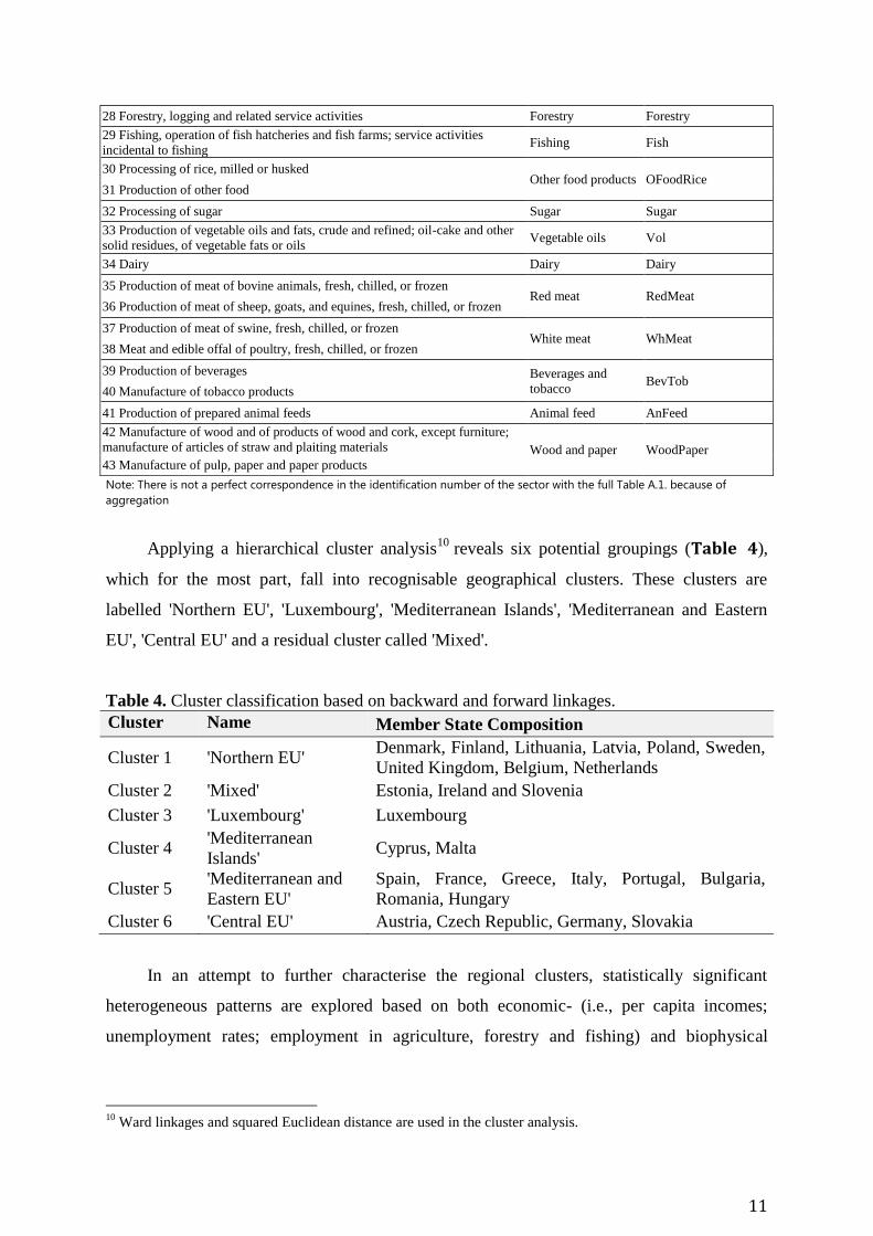
28 Forestry, logging and related service activities Forestry Forestry

29 Fishing, operation of fish hatcheries and fish farms; service activities

incidental to fishing Fishing Fish

30 Processing of rice, milled or husked Other food products OFoodRice

31 Production of other food

32 Processing of sugar Sugar Sugar

33 Production of vegetable oils and fats, crude and refined; oil-cake and other

solid residues, of vegetable fats or oils Vegetable oils Vol

34 Dairy Dairy Dairy

35 Production of meat of bovine animals, fresh, chilled, or frozen Red meat RedMeat

36 Production of meat of sheep, goats, and equines, fresh, chilled, or frozen

37 Production of meat of swine, fresh, chilled, or frozen White meat WhMeat

38 Meat and edible offal of poultry, fresh, chilled, or frozen

39 Production of beverages Beverages and

tobacco BevTob

40 Manufacture of tobacco products

41 Production of prepared animal feeds Animal feed AnFeed

42 Manufacture of wood and of products of wood and cork, except furniture;

manufacture of articles of straw and plaiting materials Wood and paper WoodPaper

43 Manufacture of pulp, paper and paper products

Note: There is not a perfect correspondence in the identification number of the sector with the full Table A.1. because of

aggregation

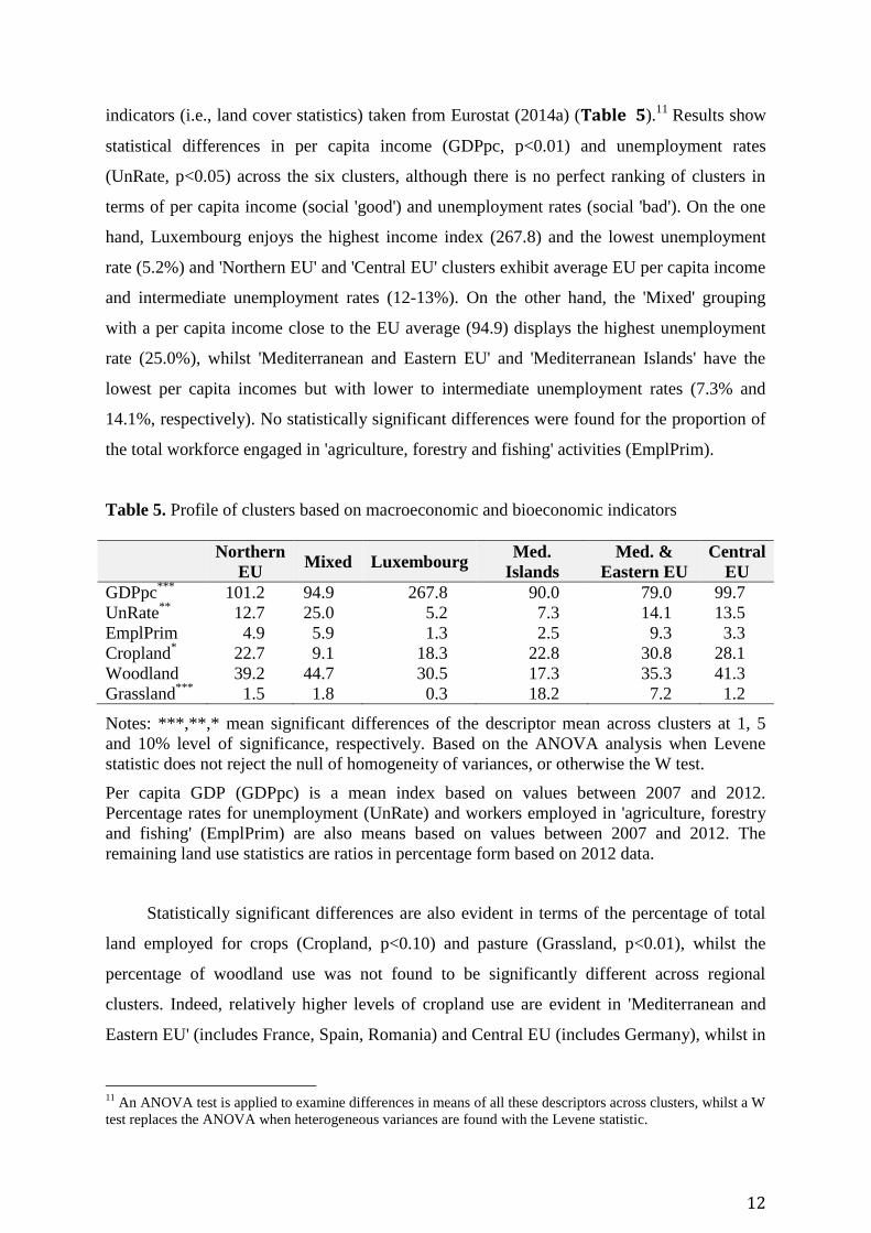
Applying a hierarchical cluster analysis10

reveals six potential groupings (Table 4),

which for the most part, fall into recognisable geographical clusters. These clusters are

labelled 'Northern EU', 'Luxembourg', 'Mediterranean Islands', 'Mediterranean and Eastern

EU', 'Central EU' and a residual cluster called 'Mixed'.

Table 4. Cluster classification based on backward and forward linkages.

Cluster Name Member State Composition

Cluster 1 'Northern EU' Denmark, Finland, Lithuania, Latvia, Poland, Sweden,

United Kingdom, Belgium, Netherlands

Cluster 2 'Mixed' Estonia, Ireland and Slovenia

Cluster 3 'Luxembourg' Luxembourg

Cluster 4 'Mediterranean

Islands' Cyprus, Malta

Cluster 5 'Mediterranean and

Eastern EU'

Spain, France, Greece, Italy, Portugal, Bulgaria,

Romania, Hungary

Cluster 6 'Central EU' Austria, Czech Republic, Germany, Slovakia

In an attempt to further characterise the regional clusters, statistically significant

heterogeneous patterns are explored based on both economic- (i.e., per capita incomes;

unemployment rates; employment in agriculture, forestry and fishing) and biophysical

10

Ward linkages and squared Euclidean distance are used in the cluster analysis.

12

indicators (i.e., land cover statistics) taken from Eurostat (2014a) (Table 5).11

Results show

statistical differences in per capita income (GDPpc, p<0.01) and unemployment rates

(UnRate, p<0.05) across the six clusters, although there is no perfect ranking of clusters in

terms of per capita income (social 'good') and unemployment rates (social 'bad'). On the one

hand, Luxembourg enjoys the highest income index (267.8) and the lowest unemployment

rate (5.2%) and 'Northern EU' and 'Central EU' clusters exhibit average EU per capita income

and intermediate unemployment rates (12-13%). On the other hand, the 'Mixed' grouping

with a per capita income close to the EU average (94.9) displays the highest unemployment

rate (25.0%), whilst 'Mediterranean and Eastern EU' and 'Mediterranean Islands' have the

lowest per capita incomes but with lower to intermediate unemployment rates (7.3% and

14.1%, respectively). No statistically significant differences were found for the proportion of

the total workforce engaged in 'agriculture, forestry and fishing' activities (EmplPrim).

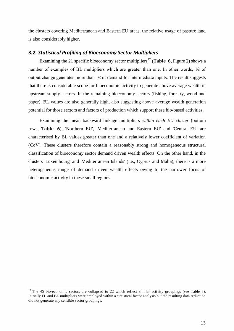
Table 5. Profile of clusters based on macroeconomic and bioeconomic indicators

Northern

EU Mixed Luxembourg

Med.

Islands

Med. &

Eastern EU

Central

EU

GDPpc***

101.2 94.9 267.8 90.0 79.0 99.7

UnRate**

12.7 25.0 5.2 7.3 14.1 13.5

EmplPrim 4.9 5.9 1.3 2.5 9.3 3.3

Cropland* 22.7 9.1 18.3 22.8 30.8 28.1

Woodland 39.2 44.7 30.5 17.3 35.3 41.3

Grassland***

1.5 1.8 0.3 18.2 7.2 1.2

Notes: ***,**,* mean significant differences of the descriptor mean across clusters at 1, 5

and 10% level of significance, respectively. Based on the ANOVA analysis when Levene

statistic does not reject the null of homogeneity of variances, or otherwise the W test.

Per capita GDP (GDPpc) is a mean index based on values between 2007 and 2012.

Percentage rates for unemployment (UnRate) and workers employed in 'agriculture, forestry

and fishing' (EmplPrim) are also means based on values between 2007 and 2012. The

remaining land use statistics are ratios in percentage form based on 2012 data.

Statistically significant differences are also evident in terms of the percentage of total

land employed for crops (Cropland, p<0.10) and pasture (Grassland, p<0.01), whilst the

percentage of woodland use was not found to be significantly different across regional

clusters. Indeed, relatively higher levels of cropland use are evident in 'Mediterranean and

Eastern EU' (includes France, Spain, Romania) and Central EU (includes Germany), whilst in

11

An ANOVA test is applied to examine differences in means of all these descriptors across clusters, whilst a W

test replaces the ANOVA when heterogeneous variances are found with the Levene statistic.

13

the clusters covering Mediterranean and Eastern EU areas, the relative usage of pasture land

is also considerably higher.

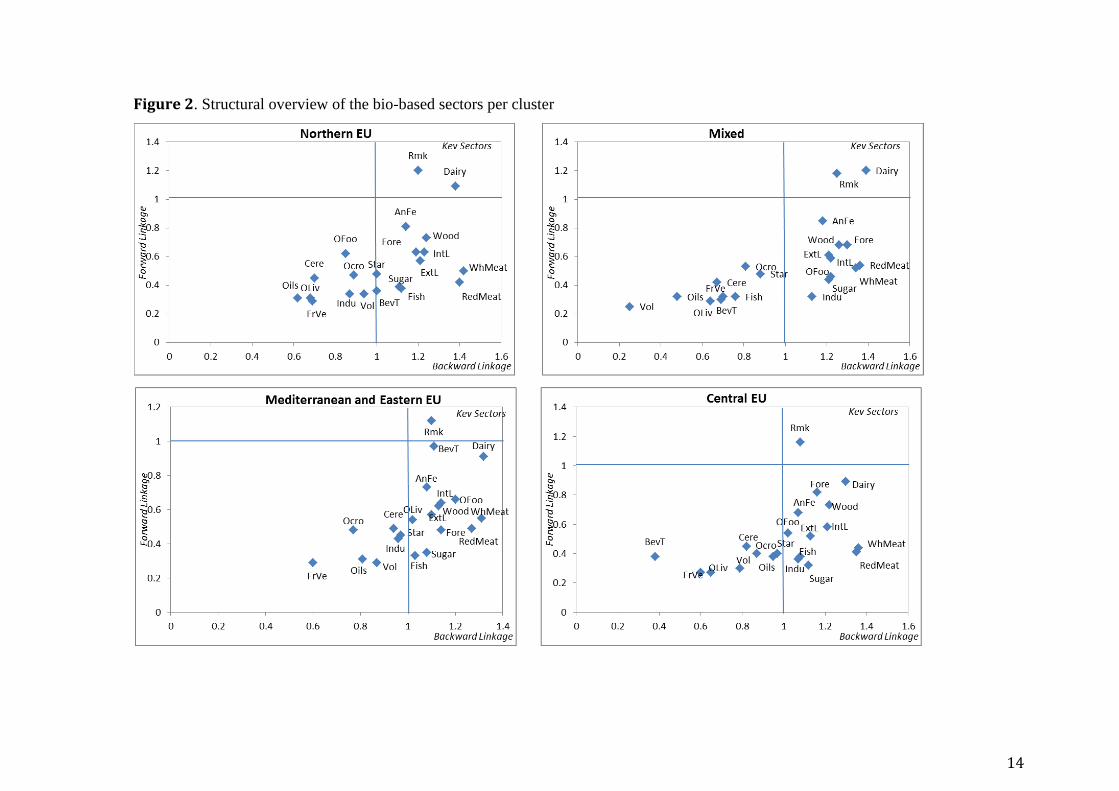
3.2. Statistical Profiling of Bioeconomy Sector Multipliers

Examining the 21 specific bioeconomy sector multipliers12

(Table 6, Figure 2) shows a

number of examples of BL multipliers which are greater than one. In other words, 1€ of

output change generates more than 1€ of demand for intermediate inputs. The result suggests

that there is considerable scope for bioeconomic activity to generate above average wealth in

upstream supply sectors. In the remaining bioeconomy sectors (fishing, forestry, wood and

paper), BL values are also generally high, also suggesting above average wealth generation

potential for those sectors and factors of production which support these bio-based activities.

Examining the mean backward linkage multipliers within each EU cluster (bottom

rows, Table 6), 'Northern EU', 'Mediterranean and Eastern EU' and 'Central EU' are

characterised by BL values greater than one and a relatively lower coefficient of variation

(CoV). These clusters therefore contain a reasonably strong and homogeneous structural

classification of bioeconomy sector demand driven wealth effects. On the other hand, in the

clusters 'Luxembourg' and 'Mediterranean Islands' (i.e., Cyprus and Malta), there is a more

heterogeneous range of demand driven wealth effects owing to the narrower focus of

bioeconomic activity in these small regions.

12

The 45 bio-economic sectors are collapsed to 22 which reflect similar activity groupings (see Table 3).

Initially FL and BL multipliers were employed within a statistical factor analysis but the resulting data reduction

did not generate any sensible sector groupings.

14

Figure 2. Structural overview of the bio-based sectors per cluster

15

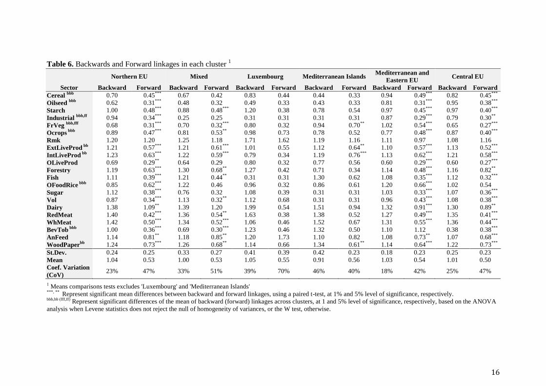
In contrast, low FL multipliers across bioeconomic sectors within each EU cluster

(Table 6) demonstrate that the level of per unit activity required to process and distribute one

unit of a given bio-economic sector's output to end users is limited. Examining the FL

multipliers within each of the six clusters (bottom rows, Table 6), the mean values are

remarkably uniform, whilst CoVs are generally higher (vis-à-vis BL multipliers) implying

that supply driven wealth effects across different bioeconomic activities are more varied.

16

Table 6. Backwards and Forward linkages in each cluster 1

Northern EU Mixed Luxembourg Mediterranean Islands Mediterranean and

Eastern EU Central EU

Sector Backward Forward Backward Forward Backward Forward Backward Forward Backward Forward Backward Forward

Cereal bbb

0.70 0.45***

0.67 0.42 0.83 0.44 0.44 0.33 0.94 0.49***

0.82 0.45***

Oilseed bbb

0.62 0.31***

0.48 0.32 0.49 0.33 0.43 0.33 0.81 0.31***

0.95 0.38***

Starch 1.00 0.48***

0.88 0.48***

1.20 0.38 0.78 0.54 0.97 0.45***

0.97 0.40***

Industrial bbb,ff

0.94 0.34***

0.25 0.25 0.31 0.31 0.31 0.31 0.87 0.29***

0.79 0.30**

FrVeg bbb,fff

0.68 0.31***

0.70 0.32***

0.80 0.32 0.94 0.70**

1.02 0.54***

0.65 0.27***

Ocrops bbb

0.89 0.47***

0.81 0.53**

0.98 0.73 0.78 0.52 0.77 0.48***

0.87 0.40***

Rmk 1.20 1.20 1.25 1.18 1.71 1.62 1.19 1.16 1.11 0.97 1.08 1.16

ExtLiveProd bb

1.21 0.57***

1.21 0.61***

1.01 0.55 1.12 0.64**

1.10 0.57***

1.13 0.52***

IntLiveProd bb

1.23 0.63***

1.22 0.59***

0.79 0.34 1.19 0.76***

1.13 0.62***

1.21 0.58***

OLiveProd 0.69 0.29**

0.64 0.29 0.80 0.32 0.77 0.56 0.60 0.29***

0.60 0.27***

Forestry 1.19 0.63

*** 1.30 0.68

** 1.27 0.42 0.71 0.34 1.14 0.48

*** 1.16 0.82

**

Fish 1.11 0.39***

1.21 0.44**

0.31 0.31 1.30 0.62 1.08 0.35***

1.12 0.32***

OFoodRice bbb

0.85 0.62***

1.22 0.46 0.96 0.32 0.86 0.61 1.20 0.66***

1.02 0.54

Sugar 1.12 0.38

*** 0.76 0.32 1.08 0.39 0.31 0.31 1.03 0.33

*** 1.07 0.36

***

Vol 0.87 0.34***

1.13 0.32**

1.12 0.68 0.31 0.31 0.96 0.43***

1.08 0.38***

Dairy 1.38 1.09

** 1.39 1.20 1.99 0.54 1.51 0.94 1.32 0.91

*** 1.30 0.89

**

RedMeat 1.40 0.42***

1.36 0.54**

1.63 0.38 1.38 0.52 1.27 0.49***

1.35 0.41***

WhMeat 1.42 0.50***

1.34 0.52***

1.06 0.46 1.52 0.67 1.31 0.55***

1.36 0.44***

BevTob bbb

1.00 0.36***

0.69 0.30***

1.23 0.46 1.32 0.50 1.10 1.12 0.38 0.38***

AnFeed 1.14 0.81**

1.18 0.85**

1.20 1.73 1.10 0.82 1.08 0.73**

1.07 0.68***

WoodPaperbb

1.24 0.73***

1.26 0.68**

1.14 0.66 1.34 0.61**

1.14 0.64***

1.22 0.73***

St.Dev. 0.24 0.25 0.33 0.27 0.41 0.39 0.42 0.23 0.18 0.23 0.25 0.23

Mean 1.04 0.53 1.00 0.53 1.05 0.55 0.91 0.56 1.03 0.54 1.01 0.50

Coef. Variation

(CoV) 23% 47% 33% 51% 39% 70% 46% 40% 18% 42% 25% 47%

1 Means comparisons tests excludes 'Luxembourg' and 'Mediterranean Islands'

***, ** Represent significant mean differences between backward and forward linkages, using a paired t-test, at 1% and 5% level of significance, respectively.

bbb,bb (fff,ff) Represent significant differences of the mean of backward (forward) linkages across clusters, at 1 and 5% level of significance, respectively, based on the ANOVA

analysis when Levene statistics does not reject the null of homogeneity of variances, or the W test, otherwise.

17

Interestingly, animal related (i.e., meat, livestock, milk, dairy and animal feed sectors),

'wood and paper' and 'forestry' sectors in (almost) all clusters have significant buyer

generating wealth potential (i.e., mean BL multipliers greater than one). By contrast,

cropping activities (i.e., industrial crops, other crops, cereals, fruit and vegetables, oilseeds)

have mean BL multipliers of less than one in all clusters. In terms of FL mean multipliers,

only dairy and raw milk sectors have values which are consistently close to, or above one.

Additional statistical tests focus on identifying bioeconomic structural heterogeneity

across the six clusters. In other words, the aim is to understand the extent (if any) to which

demand and supply driven wealth generation in a given bioeconomic sector differs across the

EU region clusters. Thus, a paired t-test (5% significance) is conducted in order to ascertain

the presence of a statistically significant difference in the mean BL and FL for each of the 21

sectors (Table 6).13

Of the 21 bio-economic sectors under consideration, there are numerous

examples of statistically significant differences between mean FL and BL values in 'Northern

EU' (21 sectors), 'Mediterranean and Eastern EU' (20 sectors), 'Central EU' (20 sectors) and

in the 'Mixed' grouping (14 sectors), owing to the pervasiveness of relatively higher BLs

discussed above. The only exception to this trend appears to be the 'Mediterranean Islands'

where relatively stronger BL mean multipliers are restricted to 'fruit and vegetables', both

livestock sectors and 'wood and paper'. Interestingly, the statistically significant difference in

the mean FL and BL multipliers in five of the six clusters for these four specific bio-

economic activities confirms that the bioeconomy has a high degree of 'backward

orientation'.

Furthermore, two sets of one-way ANOVA tests focus on the differences in the BL

mean multiplier by sector and the FL mean multiplier by sector comparing across the six EU

country clusters. Of the 21 sectors, 16 (six) sectors show statistically significant structural

differences in the BL (FL) across the six clusters (not shown). Notwithstanding, repeating the

test across only four clusters (excluding 'Luxembourg' and 'Mediterranean Islands', which

between them include only three EU members with less than 1% of EU27 Gross Domestic

Product), the degree of statistical significance falls to only ten and two sectors for BL and FL

multiplier means, respectively (Table 5).14

In other words, bioeconomic BL (FL) wealth

13

In group 3, there is only one observation per sector (i.e. Luxembourg), so this test is not performed. 14

This result suggests that Luxembourg, Cyprus and Malta are structural outliers which increases the tendency

to reject the null hypothesis (i.e. means are equal) across the six groups. For example, in the case of fish (both

FL and BL multipliers) Luxembourg has no industry, whilst for the Cyprus and Malta cluster, as expected, these

sectors are (relatively speaking) strategically more important compared with the other clusters.

18

generation on a sector-by-sector basis is statistically homogeneous in 12 (20) of the 21

sectors considered.

Examining the four clusters of EU Member States, there is a statistically significant

heterogeneity in BL wealth generation for 'cereals', 'oilseeds', 'industrial crops', 'fruit and

vegetables', 'other crops', 'extensive livestock', 'intensive livestock', 'other food and rice',

'beverages and tobacco' and 'wood and paper'. A closer look reveals that in 'cereals', 'oilseeds',

'industrial crops' and 'other crops' sectors, the strongest BL multipliers are reported in the

'Mediterranean and Eastern EU' and 'Central EU' clusters. On the other hand, the

'Mediterranean and Eastern EU' cluster contains relatively stronger BL multipliers in 'fruit

and vegetables'. In intensive and extensive livestock activities, whilst BL multipliers are

strong in all four clusters, 'Northern EU' and 'Mixed' clusters exhibit the strongest BL

multipliers across the two sectors, whereas in the beverages and tobacco sectors, 'Mixed' and

'Central EU' have very weak BL multipliers. Finally, in 'wood and paper', 'Northern EU',

'Mixed' and 'Central EU' clusters exhibit the strongest BL multipliers. In two of the

aforementioned ten sectors ('industrial crops' and 'fruit and vegetables'), there is also

statistically significant heterogeneity across the four EU clusters in terms of FL wealth

generation. This suggests that both sectors have very disparate input-output structures across

the EU.

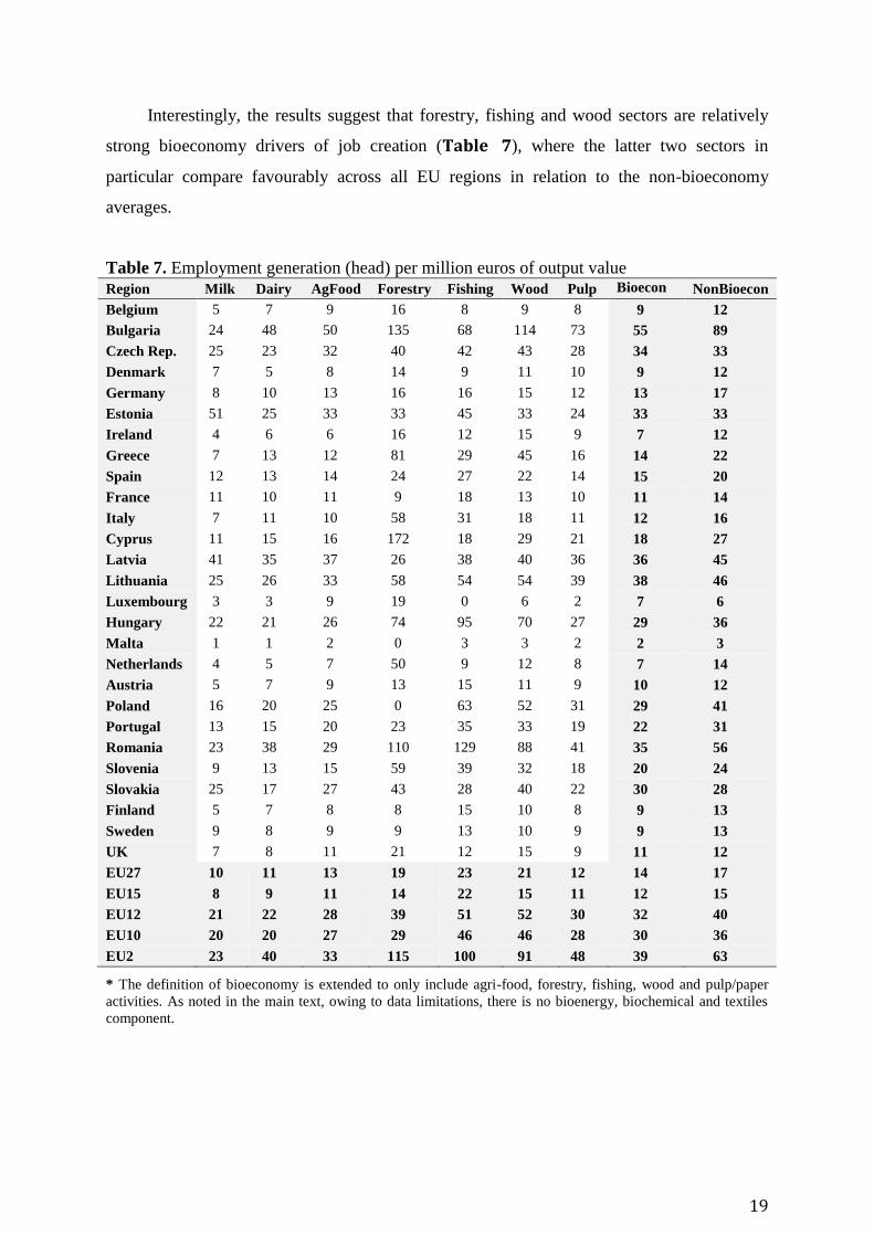
3.3. Bioeconomy Employment Multipliers

Employment multipliers are presented in Table 7, defined as the number of new jobs

generated per million euros of additional output value (see appendix for details). Calculations

are presented for raw milk and dairy (see next subsection), forestry, fishing, wood, pulp and

the aggregate sectors 'agri-food' and 'bioeconomy'.15

In Figure 3, a summary of these figures

for alternative aggregation of Member States is presented.

For the EU27, the employment multiplier analysis suggests the creation of 14 new posts

for every million euros of additional bioeconomic output value.16

In comparison, the

corresponding EU27 average for non-bioeconomy sectors reveals a slightly higher level of

job creation (17 jobs/million euros). This finding is broadly robust across all EU27 Member

States (except for the Czech Republic, Luxembourg and Slovakia), whilst in the 2007 Balkan

accession members (EU2), non bioeconomy job creation is notably higher.

15

Given the relative output value share weight of agri-food activity within the definition of bioeconomy

employed here, the multipliers in both aggregates move closely together. 16

Note that the broadness of the definition of bioeconomy is limited in this study

19

Interestingly, the results suggest that forestry, fishing and wood sectors are relatively

strong bioeconomy drivers of job creation (Table 7), where the latter two sectors in

particular compare favourably across all EU regions in relation to the non-bioeconomy

averages.

Table 7. Employment generation (head) per million euros of output value

Region Milk Dairy AgFood Forestry Fishing Wood Pulp Bioecon

* NonBioecon

Belgium 5 7 9 16 8 9 8 9 12

Bulgaria 24 48 50 135 68 114 73 55 89

Czech Rep. 25 23 32 40 42 43 28 34 33

Denmark 7 5 8 14 9 11 10 9 12

Germany 8 10 13 16 16 15 12 13 17

Estonia 51 25 33 33 45 33 24 33 33

Ireland 4 6 6 16 12 15 9 7 12

Greece 7 13 12 81 29 45 16 14 22

Spain 12 13 14 24 27 22 14 15 20

France 11 10 11 9 18 13 10 11 14

Italy 7 11 10 58 31 18 11 12 16

Cyprus 11 15 16 172 18 29 21 18 27

Latvia 41 35 37 26 38 40 36 36 45

Lithuania 25 26 33 58 54 54 39 38 46

Luxembourg 3 3 9 19 0 6 2 7 6

Hungary 22 21 26 74 95 70 27 29 36

Malta 1 1 2 0 3 3 2 2 3

Netherlands 4 5 7 50 9 12 8 7 14

Austria 5 7 9 13 15 11 9 10 12

Poland 16 20 25 0 63 52 31 29 41

Portugal 13 15 20 23 35 33 19 22 31

Romania 23 38 29 110 129 88 41 35 56

Slovenia 9 13 15 59 39 32 18 20 24

Slovakia 25 17 27 43 28 40 22 30 28

Finland 5 7 8 8 15 10 8 9 13

Sweden 9 8 9 9 13 10 9 9 13

UK 7 8 11 21 12 15 9 11 12

EU27 10 11 13 19 23 21 12 14 17

EU15 8 9 11 14 22 15 11 12 15

EU12 21 22 28 39 51 52 30 32 40

EU10 20 20 27 29 46 46 28 30 36

EU2 23 40 33 115 100 91 48 39 63

* The definition of bioeconomy is extended to only include agri-food, forestry, fishing, wood and pulp/paper

activities. As noted in the main text, owing to data limitations, there is no bioenergy, biochemical and textiles

component.

20

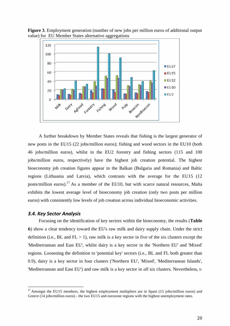
Figure 3. Employment generation (number of new jobs per million euros of additional output

value) for EU Member States alternative aggregations

A further breakdown by Member States reveals that fishing is the largest generator of

new posts in the EU15 (22 jobs/million euros); fishing and wood sectors in the EU10 (both

46 jobs/million euros), whilst in the EU2 forestry and fishing sectors (115 and 100

jobs/million euros, respectively) have the highest job creation potential. The highest

bioeconomy job creation figures appear in the Balkan (Bulgaria and Romania) and Baltic

regions (Lithuania and Latvia), which contrasts with the average for the EU15 (12

posts/million euros).17

As a member of the EU10, but with scarce natural resources, Malta

exhibits the lowest average level of bioeconomy job creation (only two posts per million

euros) with consistently low levels of job creation across individual bioeconomic activities.

3.4. Key Sector Analysis

Focusing on the identification of key sectors within the bioeconomy, the results (Table

6) show a clear tendency toward the EU's raw milk and dairy supply chain. Under the strict

definition (i.e., BL and FL > 1), raw milk is a key sector in five of the six clusters except the

'Mediterranean and East EU', whilst dairy is a key sector in the 'Northern EU' and 'Mixed'

regions. Loosening the definition to 'potential key' sectors (i.e., BL and FL both greater than

0.9), dairy is a key sector in four clusters ('Northern EU', 'Mixed', 'Mediterranean Islands',

'Mediterranean and East EU') and raw milk is a key sector in all six clusters. Nevertheless, t-

17

Amongst the EU15 members, the highest employment multipliers are in Spain (15 jobs/million euros) and

Greece (14 jobs/million euros) - the two EU15 and eurozone regions with the highest unemployment rates.

21

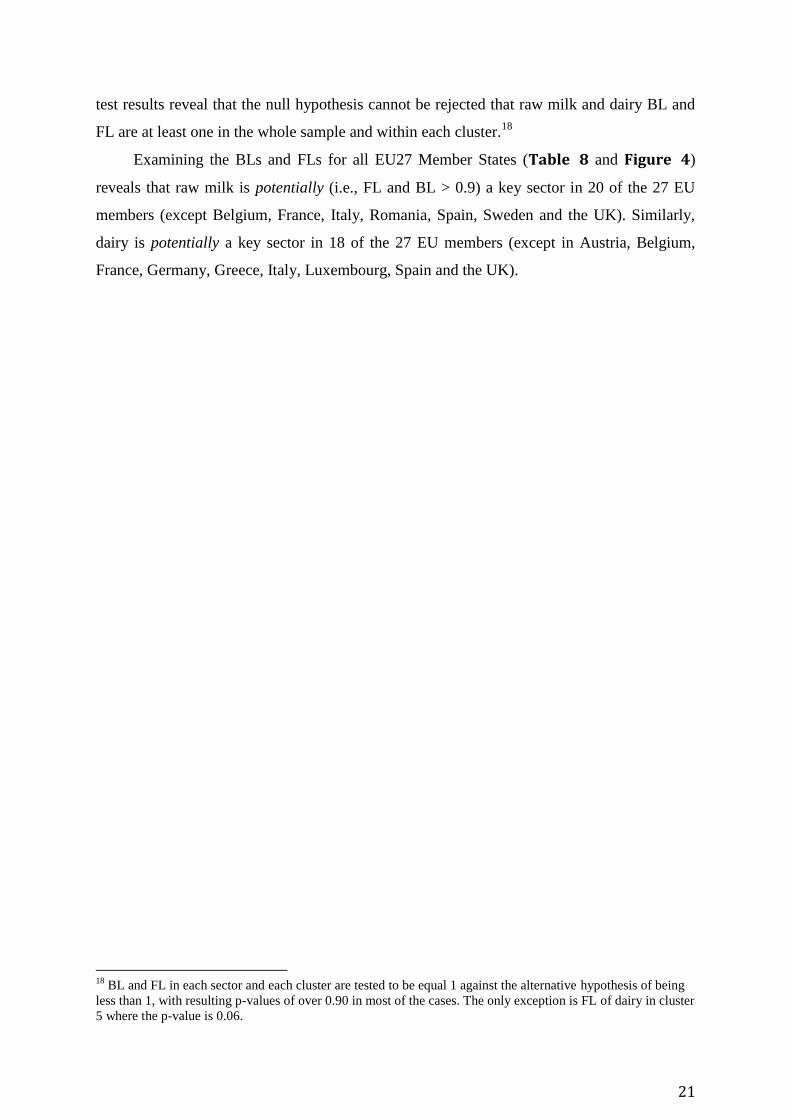
test results reveal that the null hypothesis cannot be rejected that raw milk and dairy BL and

FL are at least one in the whole sample and within each cluster.18

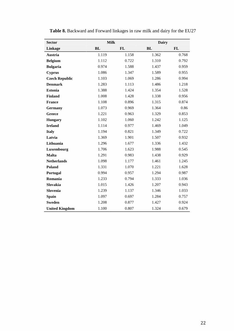
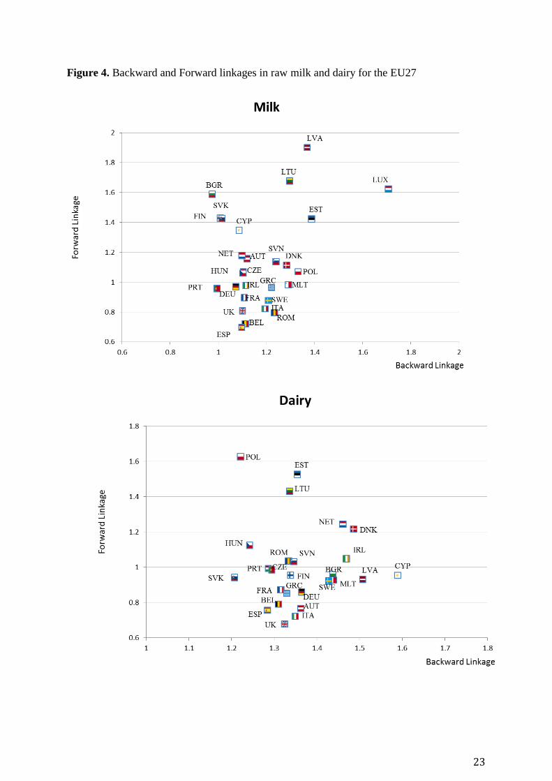
Examining the BLs and FLs for all EU27 Member States (Table 8 and Figure 4)

reveals that raw milk is potentially (i.e., FL and BL > 0.9) a key sector in 20 of the 27 EU

members (except Belgium, France, Italy, Romania, Spain, Sweden and the UK). Similarly,

dairy is potentially a key sector in 18 of the 27 EU members (except in Austria, Belgium,

France, Germany, Greece, Italy, Luxembourg, Spain and the UK).

18

BL and FL in each sector and each cluster are tested to be equal 1 against the alternative hypothesis of being

less than 1, with resulting p-values of over 0.90 in most of the cases. The only exception is FL of dairy in cluster

5 where the p-value is 0.06.

22

Table 8. Backward and Forward linkages in raw milk and dairy for the EU27

Sector Milk Dairy

Linkage BL FL BL FL

Austria 1.119 1.158 1.362 0.768

Belgium 1.112 0.722 1.310 0.792

Bulgaria 0.974 1.588 1.437 0.959

Cyprus 1.086 1.347 1.589 0.955

Czech Republic 1.103 1.069 1.286 0.994

Denmark 1.283 1.113 1.486 1.218

Estonia 1.388 1.424 1.354 1.528

Finland 1.008 1.428 1.338 0.956

France 1.108 0.896 1.315 0.874

Germany 1.073 0.969 1.364 0.86

Greece 1.221 0.963 1.329 0.853

Hungary 1.102 1.060 1.242 1.125

Ireland 1.114 0.977 1.469 1.049

Italy 1.194 0.821 1.349 0.722

Latvia 1.369 1.901 1.507 0.932

Lithuania 1.296 1.677 1.336 1.432

Luxembourg 1.706 1.623 1.988 0.545

Malta 1.291 0.983 1.438 0.929

Netherlands 1.098 1.177 1.461 1.245

Poland 1.331 1.070 1.221 1.628

Portugal 0.994 0.957 1.294 0.987

Romania 1.233 0.794 1.333 1.036

Slovakia 1.015 1.426 1.207 0.943

Slovenia 1.239 1.137 1.346 1.033

Spain 1.097 0.697 1.284 0.757

Sweden 1.208 0.877 1.427 0.924

United Kingdom 1.100 0.807 1.324 0.679

23

Figure 4. Backward and Forward linkages in raw milk and dairy for the EU27

24

The employment multipliers for raw milk and dairy exhibit a similar regional pattern

highlighted in the previous section. More specifically, higher multipliers are positively

correlated with those EU members with lower per capita incomes. The highest employment

multipliers in raw milk are found in the Baltic regions of Estonia (51 posts/million euros of

value) and Latvia (41 posts/million euros of value), whilst in dairy the highest employment

multipliers are exhibited in the Balkan regions of Bulgaria (48 posts/million euros of value)

and Romania (38 posts/million euros of value), as well as Latvia (35 posts/million euros of

value). Importantly, comparing with the agri-food and bioeconomy sector averages (Table

8), the level of job creation in raw milk and dairy is, in general, lower, which reflects the

higher degree of capitalisation within these sectors.

From a policy perspective, this research suggests that for most EU members, raw milk

and dairy bio-based sectors constitute a priority in terms of wealth generation, although

neither is a strong employment generator. Notwithstanding, given the choice of benchmark

year (2007), it is interesting to conduct an ex-post analysis to ascertain the extent to which

said key sectors have performed in the ensuing period. As an initial observation, in the

financial crisis period between 2007 and 2011, Eurostat (2014a) figures reveal that the EU

dairy sector posted impressive growth of 5.5% in milk production and 4.3% in cheese. These

statistics compare with an agricultural sector increase of 2% while food industry production

witnessed a decrease of 1.7%. Indeed, despite high energy and feed prices, and the abolition

of export refunds, milk and dairy related industries continued to thrive in a climate of

economic downturn. This is due to favourable demand conditions on the world market as

well as steady improvements in cow yields (DG AGRI, 2013).

25

At the EU member state level, it is interesting to note that milk/dairy production over

the period 2007 to 2011 has fallen in those members (i.e., Bulgaria and Romania) where

milk/dairy is not considered as a key sector (DG AGRI, 2013). Equally, it is anticipated that

in the Netherlands, Denmark, Germany, Austria and Cyprus, where raw milk quota is

currently fully utilised, increases in production are expected to appear from 2015 onwards

when the quota is abolished (DG AGRI, 2013). In all of these EU members, except Germany,

the current research identifies raw milk as a key sector, whilst in Germany, raw milk is a

potential key sector (Table 7). Moreover, the largest growth in cheese production between

2007 and 2013, which is the industry which provides the highest value added to collected

milk, comes from Estonia, Lithuania and Poland (DG AGRI, 2013). Examining the results of

the current paper, the dairy sector in each of these three members is a key sector, with the

highest dairy FL multipliers of all the 27 EU members (Table 8).

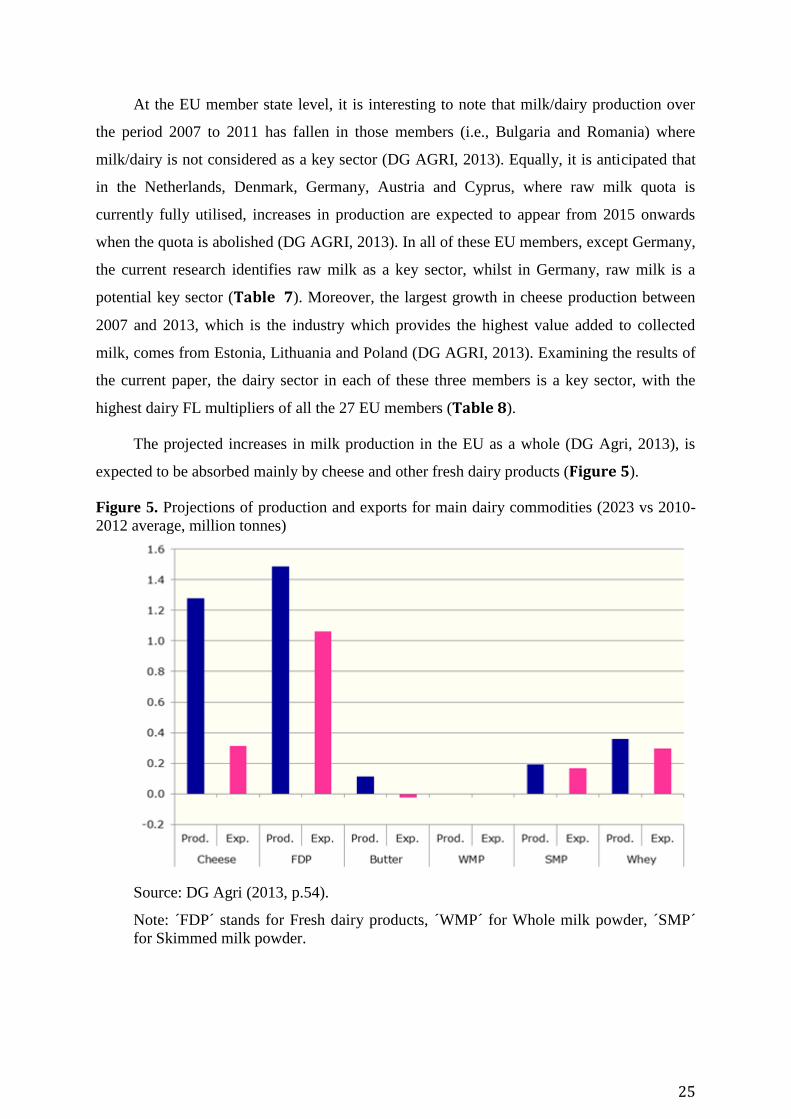
The projected increases in milk production in the EU as a whole (DG Agri, 2013), is

expected to be absorbed mainly by cheese and other fresh dairy products (Figure 5).

Figure 5. Projections of production and exports for main dairy commodities (2023 vs 2010-

2012 average, million tonnes)

Source: DG Agri (2013, p.54).

Note: ´FDP´ stands for Fresh dairy products, ´WMP´ for Whole milk powder, ´SMP´

for Skimmed milk powder.

26

4. Conclusions

The creation of the EU's bioeconomy strategy (EC, 2012) reflects a broader attempt by

EU policy makers to engage in a process of responsible resource usage whilst fostering

economic growth. In particular, the remit of this strategy includes the optimisation of

biological resources including waste, reduced dependency on fossil fuels and lowering the

negative economic growth inducing impacts on the environment (EC, 2014a). Quantitative

approaches to measuring bioeconomic activity are constrained by a shortage of available

published data, which consequently narrows the definition of bioeconomy in this study.

Notwithstanding, as a partial response, a consistent set of social accounting matrices (SAMs)

for each of the 27 EU Member States updated to 2007, known as the AgroSAMs (Müller et

al., 2009), is employed, with a highly detailed representation of agricultural and food sectors,

in addition to fishing, forestry, wood and paper/pulp activities.

Employing backward-linkage (BL) and forward-linkage (FL) multipliers as segmenting

variables, a cluster analysis generates six groupings of EU member with homogeneous

bioeconomic wealth generation properties, broadly clear geographical distinctions, and

statistically significant heterogeneity between groups in terms of economic development and

land use variables. Hence, a potential link is forged between bioeconomic structure,

geographical location and relative economic development. Furthermore, within cluster

statistical tests reveal a uniformly high degree of 'backward orientation' or backward wealth

generation across bioeconomic sectors. In the agro-food sectors, this interpretation is

rationalised by the reliance on a diverse portfolio of inputs (e.g. fertilisers, pesticides,

veterinary services, machinery, transport services, energy requirements etc.) which generate,

in relative terms, greater than average economic ripple effects through the rest of the

economy. Furthermore, in developed economies and the EU in particular, high BLs owing to

highly diversified input requirements are perhaps to be expected given the strict legal

regulations regarding food standards, food safety requirements and animal welfare. By the

same token, the implication of low FL wealth generation is that the supply chain for

bioeconomic outputs is less dispersed, thereby leading to smaller ripple effects. For example,

in many cases, bioeconomic outputs remain as unprocessed or raw goods, and therefore do

not have many alternative uses.

Additional inter-cluster statistical comparisons by bioeconomic sector show only a

moderate degree of heterogeneity in terms of BL wealth generation. Performing the same test

for FL multipliers reduces the statistical degree of structural heterogeneity to only two

27

sectors. In the case of the industrial crops sector (predominantly sugar beet), the result is

supported by earlier literature (Renwick et al., 2011) showing notable differences in sugar

beet competitiveness across the EU.19

A similar argument could be made for fruit and

vegetable production, which owing to climatic factors, is concentrated in the hands of those

EU-members on the northern basin of the Mediterranean.20

Comparing with the non-bioeconomic sector aggregate, the bioeconomy generates

relatively less employment. On the other hand, comparatively favourable levels of bio-based

employment growth can be found in the forestry, fishing21

and wood industries, whilst an

inverse relationship is found between lower economic development (per capita income) and

higher bioeconomy employment generation. Finally, the bio-based sectors of milk and dairy

are found to be significant wealth generators, although their employment generation is below

the agri-food average. Furthermore, analysing the evolution of milk and dairy markets since

2007 reveals a striking congruence between the policy recommendations of this research and

the positive ex-post evolution of milk and dairy sectors in certain EU Member States.

An initial caveat to this research is that it cannot make informed judgements on the

environmental sustainability relating to the policy recommendations (i.e., key sectors) within

this study. For example, although milk and dairy are strategic bio-based wealth generators,

the incremental harm to the environment (i.e., enteric fermentation, manure management)

may have notable consequences when respecting emissions limits. In addition, whilst the

employment multipliers are intuitively appealing, when comparing between sectors and EU

regions, one cannot make strong inferences between the number of head employed and the

resulting impact on labour income generation and economic growth, since there is no a priori

indication of the relative 'quality' of the labour force. Importantly, in the poorer members

there is a higher job creation elasticity to bioeconomic output value changes which (in part)

suggests a higher labour (lower capital) intensive production technology in these sectors,

much of which may be lower skilled; less productive and/or with a lower remuneration.

A final cautionary note relates to the selective bioeconomic focus on agri-food,

forestry, fishing, wood and paper/pulp activities, which are typically identified in the standard

19

Competitive differences owe as much to institutional arrangements between beet suppliers and processors as

well as agronomic and climatic factors. The relatively competitive cluster groups are 'Northern Europe' (UK,

Sweden, Netherlands, Finland, Denmark, Poland); 'Mediterranean and Eastern Europe' (France and Hungary);

and 'Central Europe' (Slovakia, Germany, Austria). 20

The strategic importance of Belgian and Dutch vegetable sectors is lost within the large EU cluster of

'Northern Europe' where the multiplier impact of the fruit and vegetable sector is representative of nine Member

States. 21

Given that fishing activity is constrained by quotas, most job creation would likely occur through aquaculture,

where the Commission intends to boost production by reforming the Common Fisheries Policy (EC, 2014b).

28

system of national accounts. The agri-food sectors are disaggregated, although there remain

significant areas of bio-based activity which remain 'hidden' within the official EU national

accounts statistics. To further illustrate the policy relevance of this point, the 'cascading

principle' (EP, 2013) posits that the usage of biomass should flow from higher levels of the

value chain down to lower levels, thereby maximising the productivity of the raw material.

Within this guiding paradigm, the use of biomass for energy generation is placed at the end of

the cascade. Thus, whilst the multiplier approach could lend itself to test the cascading

biomass hypothesis by comparing BL and FL multipliers (i.e., wealth generation properties)

across an all-encompassing selection of bio-based activities, at present such an approach is

limited by data availability. Thus, a clear avenue for further research is to address this

shortfall to provide a more comprehensive depiction of this complex and diverse sector.

29

References Arndt C, Jones S, Tarp F, 2000. Structural characteristic of the economy of Mozambique: A

SAM-based analysis. Rev Dev Econ 4(3): 292-306

Britz W, Witzke HP (Eds), 2012. CAPRI model documentation 2012. Available in:

http://www.capri-model.org/docs/capri_documentation.pdf [29 April 2014]

Cardenete MA, Sancho F, 2006. Missing Links in Key Sector Analysis, Econ Syst Res 18(3):

319-326.

Defourny J, Thorbecke E, 1984. Structural Path Analysis and Multiplier Decomposition

within a Social Accounting Matrix. Econ J 94 (373): 111-136.

De Miguel-Velez FJ, Perez-Mayo J., 2010. Poverty Reduction and SAM Multipliers: An

Evaluation of Public Policies in a Regional Framework. Eur Plan Stud 18(3): 449-466

Directorate General Agriculture and Rural Development (DG AGRI), 2013. Prospects for

agricultural markets and income in the EU 2013-2023. Available in:

http://ec.europa.eu/agriculture/markets-and-prices/medium-term-

outlook/2013/fullrep_en.pdf [29 April 2014]

Dietzenbacher E, Van der Linden JA, 1997. Sectoral and Spatial Linkages in the EC

Production Structure. J Regional Sci 37(2): 235-257.

European Commission (EC), 2012. Communication from the Commission to the European

Parliament, the Council, the European Economic and Social Committee and the

Committee of the Regions. Innovating for Sustainable Growth: A Bioeconomy for

Europe. COM(2012) 60. Brussels 13.02.2012

European Parliament (EP), 2013. Report on innovating for sustainable growth: a bioeconomy

for Europe (2012/2295(INI)). Available in:

http://www.europarl.europa.eu/sides/getDoc.do?pubRef=-

//EP//NONSGML+REPORT+A7-2013-0201+0+DOC+PDF+V0//EN

Eurostat, 2014a. Eurostat economic accounts. Available in:

http://epp.eurostat.ec.europa.eu/portal/page/portal/national_accounts/introduction

Eurostat, 2014b. Eurostat concepts and definitions database. Available in:

http://ec.europa.eu/eurostat/ramon/nomenclatures/index.cfm?TargetUrl=DSP_GLOSS

ARY_NOM_DTL_VIEW&StrNom=CODED2&StrLanguageCode=EN&IntKey=2530

5523&RdoSearch=BEGIN&TxtSearch=biomass&CboTheme=&IsTer=&IntCurrentPag

e=1&ter_valid=0 [2 March 2014]

30

Eurostat, 2014c. Structural business statistics (SBS) . Available in:

http://epp.eurostat.ec.europa.eu/portal/page/portal/european_business/introduction [2

March 2014]

European Commission, 2014a. Bioeconomy Strategy. Available in:

http://ec.europa.eu/research/bioeconomy/policy/strategy_en.htm [5 March 2014]

European Commission, 2014b. Aquaculture. Available in:

http://ec.europa.eu/fisheries/cfp/aquaculture/index_en.htm [22 April 2014]

Horridge M, 2003. SAMBAL - a GEMPACK program to balance square SAMs, Technical

paper 48, submitted October 2003. Available in:

http://www.copsmodels.com/archivep.htm [29 April 2014]

M'barek R, Philippidis G, Suta C, Vinyes C, Caivano A, Ferrari E, Ronzon T, Sanjuan-Lopez

A, Santini F, 2014. Observing and analysing the Bioeconomy in the EU: Adapting data

and tools to new questions and challenges. Bio-based and Applied Economics 3(1): 83-

91.

Müller M, Perez-Dominguez I, Gay SH, 2009. Construction of Social Accounting Matrices

for the EU27 with a Disaggregated Agricultural Sector (AgroSAM). JRC Scientific and

technical Reports, JRC 53558. Available in:

http://ipts.jrc.ec.europa.eu/publications/pub.cfm?id=2679 [29 April 2014]

Pyatt G, Round J, 1979. Accounting and Fixed Price Multipliers in a Social Accounting

Matrix, Econ J 89 (356): 850-873.

Rasmussen P, 1956. Studies in Inter-Sectoral Relations. Einar Harks, Copenhagen

(Denmark), 217pp.

Renwick A, Revoredo-Ghia C, Philippidis G, Bourne M, Lang B, Reader M., 2011.

Assessment of the Impact of the 2006 EU sugar regime reforms. Final Report prepared

for the Department of Environment, Food and Rural Affairs (DEFRA).

Robinson S, 1989. Multisector Models of Developing Countries: A Survey. In: Handbook of

Development Economics (Chenery HB, Srinivasan TN, eds.). Amsterdam, North-

Holland, pp.906-932.

Robinson S, Roland-Holst D, 1988. Macroeconomic Structure and Computable General

Equilibrium Models. J Policy Model 10: 353-375.

Rocchi B, 2009. The CAP Reform Between targeting and Equity: A Structural Policy

Analysis for Italy. Eur Rev Agric Econ 36(2): 175-202

Roland-Holst D, Sancho F, 1992. Relative Income Determination in the US: A Social

Accounting Perspective. Rev Income Wealth 38(2): 311-327.

31

Roland-Holst D, Sancho F, 1995. Modeling Prices in a Sam Structure. Rev Econ Stat 77(2):

361-371

Schultz S, 1977. Approaches to Identifying Key Sectors Empirically by means of Input-

Output Analysis. J Dev Stud 14: 77-96.

Stone J.R., 1955. Input-Output and the Social Accounts. In The Structural Interdependence of

the Economy, Proceedings of an International Conference on Input-Output Analysis

(University of Pisa ed.). Varenna, J. Wiley: New York, Giuffre: Milan, pp. 155 – 172.

Waters EC, Weber BA, Holland DW, 1999. The Role of Agriculture in Oregon's Economic

base: Findings from a Social Accounting matrix, J Agr Resour Econ 24(1): 266-280

32

Appendix

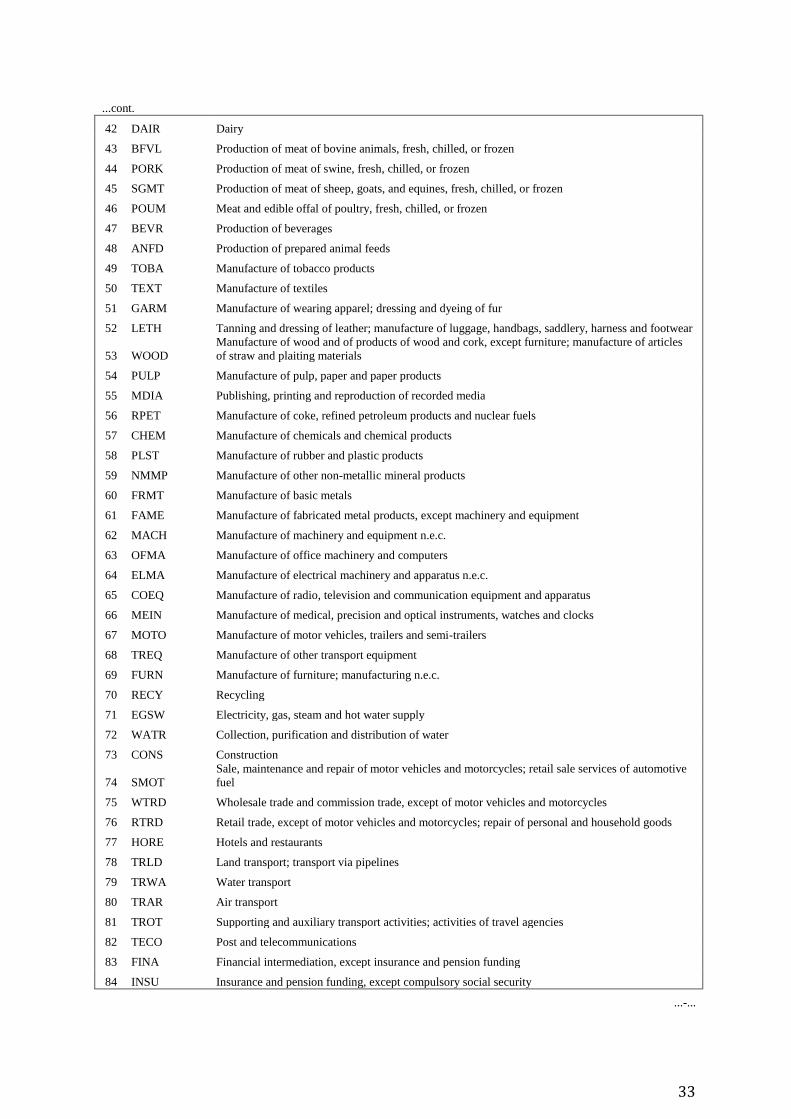
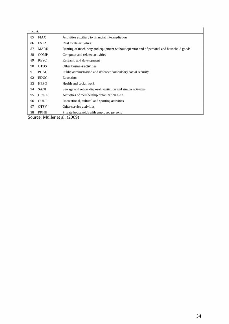
Table A.1. Sector coverage of AgroSAMS

Acronym Sector Description

1 OWHE Production of other wheat

2 DWHE Production of durum wheat

3 BARL Production of barley

4 MAIZ Production of grain maize

5 OCER Production of other cereals

6 PARI Production of paddy rice

7 RAPE Production of rape seed

8 SUNF Production of sunflower seed

9 SOYA Production of soya seed

10 OOIL Production of other oil plants

11 STPR Production of other starch and protein plants

12 POTA Production of potatoes

13 SUGB Production of sugar beet

14 FIBR Production of fibre plants

15 GRPS Production of grapes

16 FVEG Production of fresh vegetables, fruit, and nuts

17 LPLT Production of live plants

18 OTCR Other crop production activities

19 FODD Production of fodder crops

20 SETA Set aside

21 COMI Production of raw milk from bovine cattle

22 LCAT Production of bovine cattle, live

23 PIGF Production of swine, live

24 SGMI Production of raw milk from sheep and goats

25 LSGE Production of sheep, goats, horses, asses, mules and hinnies, live

26 EGGS Production of eggs

27 PLTR Production of poultry, live

28 ANHR Production of wool and animal hair; silk-worm cocoons suitable for reeling

29 OANM Production of other animals, live, and their products

30 AGSV Agricultural service activities

31 FORE Forestry, logging and related service activities

32 FISH Fishing, operation of fish hatcheries and fish farms; service activities incidental to fishing

33 COAL Mining of coal and lignite; extraction of peat

34 COIL Extraction of crude petroleum; service activities incidental to oil extraction excluding surveying

35 URAN Mining of uranium and thorium ores

36 MEOR Mining of metal ores

37 OMIN Other mining and quarrying

38 RICE Processing of rice, milled or husked

39 OFOD Production of other food

40 SUGA Processing of sugar

41 VOIL

Production of vegetable oils and fats, crude and refined; oil-cake and other solid residues, of

vegetable fats or oils

...-...

33

...cont.

42 DAIR Dairy

43 BFVL Production of meat of bovine animals, fresh, chilled, or frozen

44 PORK Production of meat of swine, fresh, chilled, or frozen

45 SGMT Production of meat of sheep, goats, and equines, fresh, chilled, or frozen

46 POUM Meat and edible offal of poultry, fresh, chilled, or frozen

47 BEVR Production of beverages

48 ANFD Production of prepared animal feeds

49 TOBA Manufacture of tobacco products

50 TEXT Manufacture of textiles

51 GARM Manufacture of wearing apparel; dressing and dyeing of fur

52 LETH Tanning and dressing of leather; manufacture of luggage, handbags, saddlery, harness and footwear

53 WOOD

Manufacture of wood and of products of wood and cork, except furniture; manufacture of articles

of straw and plaiting materials

54 PULP Manufacture of pulp, paper and paper products

55 MDIA Publishing, printing and reproduction of recorded media

56 RPET Manufacture of coke, refined petroleum products and nuclear fuels

57 CHEM Manufacture of chemicals and chemical products

58 PLST Manufacture of rubber and plastic products

59 NMMP Manufacture of other non-metallic mineral products

60 FRMT Manufacture of basic metals

61 FAME Manufacture of fabricated metal products, except machinery and equipment

62 MACH Manufacture of machinery and equipment n.e.c.

63 OFMA Manufacture of office machinery and computers

64 ELMA Manufacture of electrical machinery and apparatus n.e.c.

65 COEQ Manufacture of radio, television and communication equipment and apparatus

66 MEIN Manufacture of medical, precision and optical instruments, watches and clocks

67 MOTO Manufacture of motor vehicles, trailers and semi-trailers

68 TREQ Manufacture of other transport equipment

69 FURN Manufacture of furniture; manufacturing n.e.c.

70 RECY Recycling

71 EGSW Electricity, gas, steam and hot water supply

72 WATR Collection, purification and distribution of water

73 CONS Construction

74 SMOT

Sale, maintenance and repair of motor vehicles and motorcycles; retail sale services of automotive

fuel

75 WTRD Wholesale trade and commission trade, except of motor vehicles and motorcycles

76 RTRD Retail trade, except of motor vehicles and motorcycles; repair of personal and household goods

77 HORE Hotels and restaurants

78 TRLD Land transport; transport via pipelines

79 TRWA Water transport

80 TRAR Air transport

81 TROT Supporting and auxiliary transport activities; activities of travel agencies

82 TECO Post and telecommunications

83 FINA Financial intermediation, except insurance and pension funding

84 INSU Insurance and pension funding, except compulsory social security

...-...

34

...cont.

85 FIAX Activities auxiliary to financial intermediation

86 ESTA Real estate activities

87 MARE Renting of machinery and equipment without operator and of personal and household goods

88 COMP Computer and related activities

89 RESC Research and development

90 OTBS Other business activities

91 PUAD Public administration and defence; compulsory social security

92 EDUC Education

93 HESO Health and social work

94 SANI Sewage and refuse disposal, sanitation and similar activities

95 ORGA Activities of membership organization n.e.c.

96 CULT Recreational, cultural and sporting activities

97 OTSV Other service activities

98 PRHH Private households with employed persons

Source: Müller et al. (2009)

35

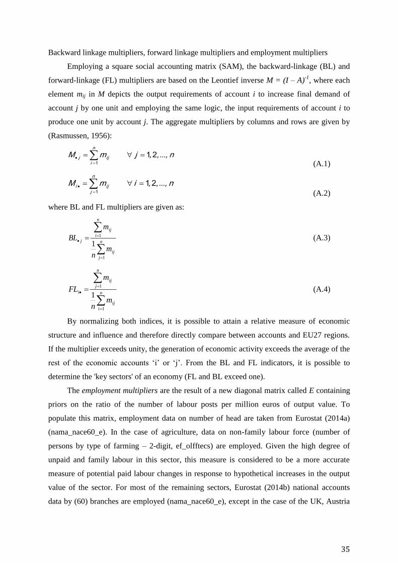
Backward linkage multipliers, forward linkage multipliers and employment multipliers

Employing a square social accounting matrix (SAM), the backward-linkage (BL) and

forward-linkage (FL) multipliers are based on the Leontief inverse M = (I – A)-1

, where each

element mij in M depicts the output requirements of account i to increase final demand of

account j by one unit and employing the same logic, the input requirements of account i to

produce one unit by account j. The aggregate multipliers by columns and rows are given by

(Rasmussen, 1956):

n

iijj n...,,,jmM

1

21 (A.1)

n

jiji n...,,,imM

1

21

(A.2)

where BL and FL multipliers are given as:

n

j

ij

n

i

ij

j

mn

m

BL

1

1

1 (A.3)

n

i

ij

n

j

ij

i

mn

m

FL

1

1

1 (A.4)

By normalizing both indices, it is possible to attain a relative measure of economic

structure and influence and therefore directly compare between accounts and EU27 regions.

If the multiplier exceeds unity, the generation of economic activity exceeds the average of the

rest of the economic accounts ‘i’ or ‘j’. From the BL and FL indicators, it is possible to

determine the 'key sectors' of an economy (FL and BL exceed one).

The employment multipliers are the result of a new diagonal matrix called E containing

priors on the ratio of the number of labour posts per million euros of output value. To

populate this matrix, employment data on number of head are taken from Eurostat (2014a)

(nama_nace60_e). In the case of agriculture, data on non-family labour force (number of

persons by type of farming – 2-digit, ef_olfftecs) are employed. Given the high degree of

unpaid and family labour in this sector, this measure is considered to be a more accurate

measure of potential paid labour changes in response to hypothetical increases in the output

value of the sector. For most of the remaining sectors, Eurostat (2014b) national accounts

data by (60) branches are employed (nama_nace60_e), except in the case of the UK, Austria

36

and Malta, where due to lack of data availability, labour data are taken from the Structural

business statistics (SBS), annual detailed enterprise statistics on industry, construction, trade

and services (Eurostat 2014c). Finally, missing observations for the forestry sector are filled

using Eurostat (2014b) data by Nace Rev 1.1 classification (for_emp_lfs1).

This matrix is multiplied by the part of the multiplicative decomposition called Ma that

incorporates the rows and columns corresponding to the productive accounts plus

endogenous accounts as labour, capital and households, in our case, and so, the multipliers

are higher than only using productive accounts. When increasing the income of an

endogenous account, one obtains the impact of said change on the corresponding column of

Ma and, via the matrix E, this is converted into the number of jobs created (or lost). The

expression of the employment multiplier, Me, is the following:

MaEMe * (A.5)

Each element in Me is the increment in the number of employment of the account i

when the account j receives a unitary exogenous injection. The sum of the columns gives the

global effect on employment resulting from an exogenous increase in demand. The rows

show the increment that the activity account in question experiences in its employment if the

rest of the accounts receive an exogenous monetary unit, i.e., the multipliers give the number

of additional jobs per million of additional output from each activity.

Europe Direct is a service to help you find answers to your questions about the European Union

Freephone number (*): 00 800 6 7 8 9 10 11

(*) Certain mobile telephone operators do not allow access to 00 800 numbers or these calls may be billed.

A great deal of additional information on the European Union is available on the Internet.

It can be accessed through the Europa server http://europa.eu.

How to obtain EU publications

Our publications are available from EU Bookshop (http://bookshop.europa.eu),

where you can place an order with the sales agent of your choice.

The Publications Office has a worldwide network of sales agents.

You can obtain their contact details by sending a fax to (352) 29 29-42758.

European Commission

EUR 26773– Joint Research Centre – Institute for Prospective Technological Studies

Title: Structural Patterns of the Bioeconomy in the EU Member States – a SAM approach

Author(s): George Philippidis; Ana I. Sanjuán; Emanuele Ferrari; Robert M'barek

Luxembourg: Publications Office of the European Union

2014 – 36 pp. – 21.0 x 29.7 cm

EUR – Scientific and Technical Research series – ISSN 1831-9424 (online)

ISBN 978-92-79-39530-7 (PDF)

doi:10.2791/10584

ISBN 978-92-79-39530-7

doi:10.2791/10584

JRC Mission As the Commission’s in-house science service, the Joint Research Centre’s mission is to provide EU policies with independent, evidence-based scientific and technical support throughout the whole policy cycle. Working in close cooperation with policy Directorates-General, the JRC addresses key societal challenges while stimulating innovation through developing new methods, tools and standards, and sharing its know-how with the Member States, the scientific community and international partners.

Serving society Stimulating innovation Supporting legislation

LF-N

A-2

67

73

-EN

-N