Structure of turbulence and sediment stratification in

RESEARCH ARTICLE10.1002/2014JC010231

Structure of turbulence and sediment stratification in wave-supported mud layersAbbas Hooshmand1, Alexander R. Horner-Devine1, and Michael P. Lamb2

1Department of Civil and Environmental Engineering, University of Washington, Seattle, Washington, USA, 2Division ofGeological and Planetary Sciences, California Institute of Technology, Pasadena, California, USA

Abstract We present results from laboratory experiments in a wave flume with and without a sedimentbed to investigate the turbulent structure and sediment dynamics of wave-supported mud layers. The pres-ence of sediment on the bed significantly alters the structure of the wave boundary layer relative to thatobserved in the absence of sediment, increasing the TKE by more than a factor of 3 at low wave orbitalvelocities and suppressing it at the highest velocities. The transition between the low and high-velocityregimes occurs when ReD ’ 450, where ReD is the Stokes Reynolds number. In the low-velocity regime(ReD < 450) the flow is significantly influenced by the formation of ripples, which enhances the TKE andReynolds stress and increases the wave boundary layer thickness. In the high-velocity regime (ReD > 450)the ripples are significantly smaller, the near-bed sediment concentrations are significantly higher and den-sity stratification due to sediment becomes important. In this regime the TKE and Reynolds stress are lowerin the sediment bed runs than in comparable runs with no sediment. The regime transition at ReD5450appears to result from washout of the ripples and increased concentrations of fine sand suspended in theboundary layer, which increases the settling flux and the stratification near the bed. The increased stratifica-tion damps turbulence, especially near the top of the high-concentration layer, reducing the layer thickness.We anticipate that these effects will influence the transport capacity of wave-supported gravity currents onthe continental shelf.

1. Introduction

Rivers carry large volumes of terrestrially derived sediments to the coast and discharge them onto the conti-nental shelf [Milliman and Meade, 1983], where they are dispersed by shelf processes [Nittrouer and Wright,1994; Wheatcroft et al., 2007]. These processes determine how sediment is redistributed on the shelf [Wrightet al., 1997, 1999, 2001] and whether it is transported off the shelf into the abyssal ocean. This latter out-come is of particular importance because it represents a flux of sediment, carbon, and nutrients out of theshelf system into the abyssal ocean where it is no longer available to the coastal ecosystem.

Once they have been discharged into shelf waters, river-borne sediment may settle near the river mouth orfurther from the mouth [Geyer et al., 2000; McPhee-Shaw et al., 2007; Walsh et al., 2004]. The sediment depo-sition depends on the ratio of sediment to freshwater discharge [Wright and Friedrichs, 2006], flocculation[Safak et al., 2013], or other processes such as convective instabilities due to particle settling in the plume[Parsons et al., 2001] that affect their removal from the plume. Once they have been deposited on the shelf,they may be moved across the shelf as turbidity currents if the shelf is steep [Hamblin and Walker, 1979; Maet al., 2008]. However, most shelves are not sufficiently steep to support seaward transport of sediment dueto gravity alone [Wright and Friedrichs, 2006]. On gently sloping shelves, additional shear from shelf currentsor surface waves is required to generate sufficient sediment suspension and maintain cross-shelf sedimenttransport. This study focuses solely on wave-generated suspensions.

Surface waves can generate significant bottom stresses on the shelf, though the stresses are strongest inshallower regions and only felt in deeper regions in storm conditions. When wave action and sediment sup-ply are sufficient, this process generates thin Oð10 cmÞ, high-concentration Oð50 g L21Þ sediment layersthat move downslope across the shelf due to gravity and are referred to as Wave-Supported Gravity Cur-rents (WSGC) [Wright and Friedrichs, 2006]. WSGCs have been observed on continental shelves near manyriver mouths, such as the Eel River [Ogston et al., 2000; Traykovski et al., 2000], Waiapu River [Ma et al., 2008],

Key Points:� Ripples dominate near-bed dynamics

in low-velocity conditions� Density stratification suppresses

turbulence in high-velocityconditions� Suspension of sand controls the

generation of high-concentrationmud layers

Correspondence to:A. R. Horner-Devine,[email protected]

Citation:Hooshmand, A., A. R. Horner-Devine,and M. P. Lamb (2015), Structure ofturbulence and sediment stratificationin wave-supported mud layers, J.Geophys. Res. Oceans, 120, 2430–2448,doi:10.1002/2014JC010231.

Received 10 JUN 2014

Accepted 12 FEB 2015

Accepted article online 18 FEB 2015

Published online 2 APR 2015

HOOSHMAND ET AL. VC 2015. American Geophysical Union. All Rights Reserved. 2430

Journal of Geophysical Research: Oceans

PUBLICATIONS

http://dx.doi.org/10.1002/2014JC010231

http://onlinelibrary.wiley.com/journal/10.1002/(ISSN)2169-9291/

http://publications.agu.org/

Po River [Traykovski et al., 2007], Atchafalaya River [Jaramillo et al., 2009], and Waipaoa River [Hale et al.,2014]. WSGCs can transport sediment seaward until the shelf is so deep that the waves do not penetrate tothe bottom and shear stress becomes small. At this point, the current may continue if the shelf is sufficientlysteep, or it will die out and the sediment will be deposited [Traykovski et al., 2000; Wright and Friedrichs,2006].

Wave-supported gravity currents are considered to be one of the primary mechanisms for cross-shelf sedi-ment transport on continental shelves [Wright and Friedrichs, 2006]. Many field observations show theimportance of these events (see previous paragraph) and a number of models have been developed basedon available field data [Wright et al., 2001; Scully et al., 2002; Traykovski et al., 2007; Falcini et al., 2012]. How-ever, field observations generally cannot resolve the structure of WSGCs in sufficient details to fully describetheir dynamics or test model assumptions. Numerical modeling [e.g., Colney et al., 2008; Ozdemir et al.,2010a] and laboratory experiments [Lamb et al., 2004; Lamb and Parsons, 2005; Liang et al., 2007; Yan et al.,2010] that can resolve the structure of these currents may provide the information necessary to improveour ability to model the transport rates in WSGCs and the conditions necessary for their formation.

Here we present new laboratory experiments that investigate the generation and turbulent structure ofhigh-density sediment suspensions over a flat bed similar to those observed on the continental shelf. Theexperiments use new instrumentation that resolves the temporal and vertical structure of the sediment andturbulent velocity fields in sufficient detail to determine the underlying physical relationships in WSGCs.The experiments and analysis focus explicitly on the competing influence of bed ripples and density stratifi-cation, in order to understand when these are important and the role they play in the dynamics of WSGCs.

2. Background

In the late 1990s, several field observations from the STRATAFORM program played a major role in improv-ing our understanding of sediment transport across continental shelves [Nittrouer, 1999; Ogston et al., 2000;Geyer et al., 2000]. Observations from the Eel River margin emphasized the important role of surface wavesin cross-shelf sediment flux and showed that a few significant storm events contributed most of the flux[Ogston et al., 2000; Puig et al., 2003]. Traykovski et al. [2000] examined the velocity and sediment concentra-tion profiles during a number of wave-induced transport events, showing that fluid mud is trapped in a thinlayer whose thickness is similar to the wave boundary layer. Although velocity measurements were not pos-sible within the mud layer, they observed enhancement of the velocity 0.5 mab relative to 1 and 2 mab dur-ing at least one major wave resuspension event and concluded that this is evidence of downslopegravitational transport. Based on the expected wave penetration, bottom slope, and depth, they concludedthat this mud layer loses energy and is deposited at a depth of 90–110 m. A series of models have beendeveloped to predict the cross-shelf flux of sediment in WSGCs, primarily based on a linearized form of theChezy equation [Wright et al., 2001; Scully et al., 2002; Traykovski et al., 2007]. Wright et al. [2001] and Scullyet al. [2002] relate sediment concentration to wave stress assuming a critical value of the bulk Richardsonnumber Rib of 0.25. However, estimates from prior laboratory experiments find that Rib is approximately anorder of magnitude smaller than this assumed value [Lamb et al., 2004], motivating a clearer understandingof the underlying dynamics in these flows.

A number of studies have used high-resolution numerical models to better understand the dynamics ofwave-generated high-concentration mud layers and to address the measurement limitations in the field[Hsu et al., 2009; Ozdemir et al., 2010a, 2011]. In agreement with the laboratory results, Hsu et al. [2009]found that Rib is smaller than 0.25, due to either a limited supply of unconsolidated fine sediment and/or astructural difference between tidal currents and wave-driven mudflows. Later Ozdemir et al. [2010b] used anumerical simulation in Eulerian-Eulerian framework for low-concentration settings and concluded that finesediments are well mixed in all phases of the wave, though turbulence is not modulated for such dilute con-centration settings. Ozdemir et al. [2010a] used the same model for a wide range of suspended sedimentconcentration (SSC) profiles with fixed wave orbital velocity. They observed a number of different regimes,including no turbulence for very dilute conditions, formation of lutocline, and finally complete laminariza-tion due to strong particle-induced stable density stratification for high sediment concentrations. Ozdemiret al. [2011] later investigated the effects of settling velocities, while maintaining constant SSC using thesame numerical model. They concluded that larger settling velocity can decrease the thickness of the high-concentration mud layer and eventually cause the flow to laminarize.

Journal of Geophysical Research: Oceans 10.1002/2014JC010231


In a series of previous laboratory experiments, Lamb et al. [2004] investigated the dynamics of high-concentration sediment suspensions with zero slope. Their study [see also Lamb and Parsons, 2005; Lianget al., 2007; Yan et al., 2010] consisted of two series of experiments; one with a rough bed without sedimentand one with a sediment bed with mostly silt size particles, representative of a continental shelf seafloor.They found that sediment reduced the thickness of the wave boundary layers substantially but that theflows were still able to support high-density suspensions thicker than the boundary layer due to upwardtransport of turbulent energy from this thin region. They also suggest that the sediment concentration inthe high-concentration layer is sufficient to generate density stratification that may influence the flowdynamics. In their experiments, Lamb et al. [2004] and Lamb and Parsons [2005] show that waves increasethe sand fraction of the near-surface bed layer through winnowing. The coarsened bed surface resulted insignificant bed load and the generation of ripples.

Such laboratory investigations of wave-supported gravity currents can bridge between simplified modelsbased on field observations and very detailed numerical models that have not been verified with fieldmeasurements. Numerical models still struggle to capture some of the physical processes that are likely tobe important in WSGCs [Hsu et al., 2009]. In particular, we expect that the range of particle sizes observed innaturally occurring flows contribute to the dynamics of the currents, through the formation of ripples, thegeneration of density stratification, and the possible interaction of these processes. Numerous studies withsand beds show that turbulence is enhanced due to ripples [Doering and Baryla, 2002; Hare et al., 2014]. Onthe other hand, work in exclusively muddy flows shows that suspended sediment can suppress turbulence[Winterwerp, 2006]. Continental shelves typically have mostly mud [Sternberg and Cacchione, 1996; Wrightet al., 1997; Kineke et al., 2000; Walsh et al., 2004] but may include a sand component (0–10%), and both rip-ples and dense suspensions have been observed [Ogston and Sternberg, 1999; Traykovski et al., 2007]. Thecompeting effects of ripples and density stratification can enhance or suppress turbulence in the water col-umn. However, it is not known under what conditions bed forms and density stratification will be importantin the sediment mixtures typical of WSGCs, whether they will coexist and under which conditions each willdominate. In this work, we will show how ripples and stratification affect the turbulence level in the waveboundary layer and determine the wave conditions in which each of them is dominant.

3. Experiments

The present experiments were carried out in a purpose-built wave-sediment U-tube tank equipped to makehigh-resolution measurements of velocity, turbulence, and suspended sediment concentration. The experi-mental facility is the same as the facility used by Lamb et al. [2004], with two important modifications. First,it has been modified to extend the upper range of wave periods from 8 to 12 s in order to better simulatewaves typically observed on the continental shelf. Second, we use new instrumentation for measuringvelocity and sediment concentration that makes high-frequency profile measurements, rather than pointmeasurements, enabling us to better resolve the turbulent wave boundary layer structure.

In order to investigate the relationship between turbulence and suspended sediment in WSGCs we carryout two parallel sets of experiments, one with an active sediment bed and one with a roughened bottomand no sediment. We compare the structure of the turbulence and sediment concentration profiles in thewave boundary layer in both cases.

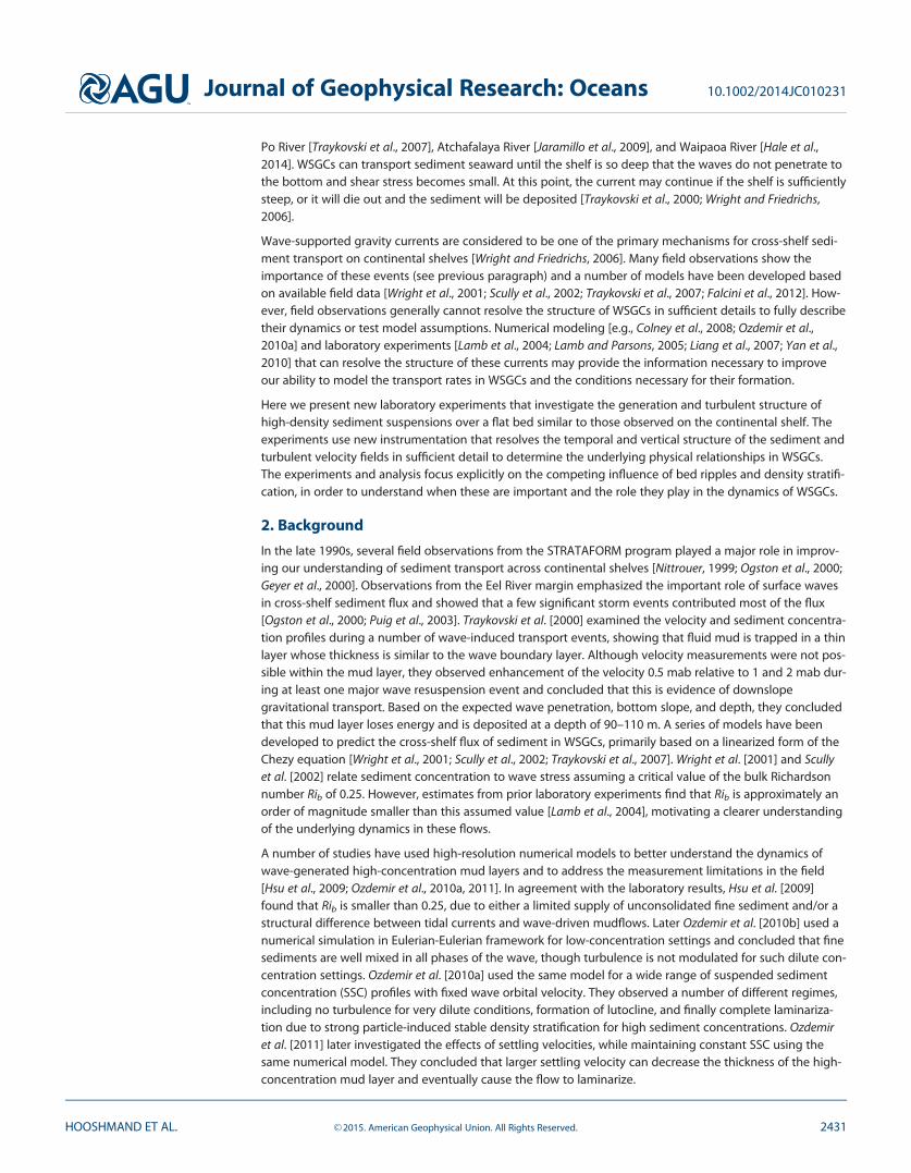
3.1. Wave FacilityThe U-tube wave facility has a sealed 5 m long, 1 m high, and 0.2 m wide test section (Figure 1). Approxi-mately, sinusoidal oscillatory flows in the test section are driven by a moving piston that produces waveswith periods of 4–12 s and orbital velocities of 20–70 cm s21. Rather than wave orbitals, the U-tube facilityproduces purely horizontal oscillatory mean flows, characteristic of the one-dimensional velocity fieldsobserved near the seabed on the continental shelf due to surface gravity waves. The top and sidewalls ofthe test section are made of smooth Plexiglas.

3.2. Rough Wall ExperimentsFor the rough wall (RW) experiments, sand particles (D505750lm) were glued to a false floor, which wasplaced on the bottom of the tank. Clear tap water was used in these experiments, which characterized theturbulent wave boundary layer flow in the absence of sediment. Overall, 20 experiments were performed in



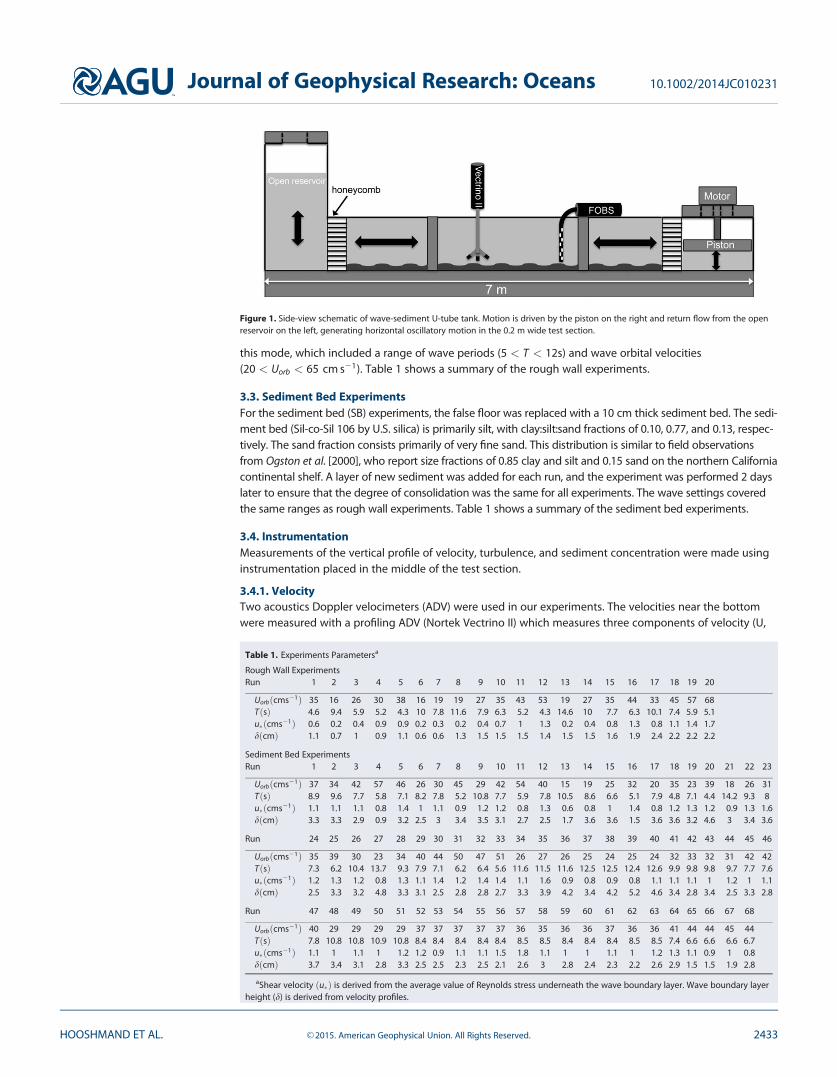
this mode, which included a range of wave periods (5 < T < 12s) and wave orbital velocities(20 < Uorb < 65 cm s21). Table 1 shows a summary of the rough wall experiments.

3.3. Sediment Bed ExperimentsFor the sediment bed (SB) experiments, the false floor was replaced with a 10 cm thick sediment bed. The sedi-ment bed (Sil-co-Sil 106 by U.S. silica) is primarily silt, with clay:silt:sand fractions of 0.10, 0.77, and 0.13, respec-tively. The sand fraction consists primarily of very fine sand. This distribution is similar to field observationsfrom Ogston et al. [2000], who report size fractions of 0.85 clay and silt and 0.15 sand on the northern Californiacontinental shelf. A layer of new sediment was added for each run, and the experiment was performed 2 dayslater to ensure that the degree of consolidation was the same for all experiments. The wave settings coveredthe same ranges as rough wall experiments. Table 1 shows a summary of the sediment bed experiments.

3.4. InstrumentationMeasurements of the vertical profile of velocity, turbulence, and sediment concentration were made usinginstrumentation placed in the middle of the test section.

3.4.1. VelocityTwo acoustics Doppler velocimeters (ADV) were used in our experiments. The velocities near the bottomwere measured with a profiling ADV (Nortek Vectrino II) which measures three components of velocity (U,

Table 1. Experiments Parametersa

Rough Wall ExperimentsRun 1 2 3 4 5 6 7 8 9 10 11 12 13 14 15 16 17 18 19 20

Uorbðcms21Þ 35 16 26 30 38 16 19 19 27 35 43 53 19 27 35 44 33 45 57 68TðsÞ 4.6 9.4 5.9 5.2 4.3 10 7.8 11.6 7.9 6.3 5.2 4.3 14.6 10 7.7 6.3 10.1 7.4 5.9 5.1u�ðcms21Þ 0.6 0.2 0.4 0.9 0.9 0.2 0.3 0.2 0.4 0.7 1 1.3 0.2 0.4 0.8 1.3 0.8 1.1 1.4 1.7dðcmÞ 1.1 0.7 1 0.9 1.1 0.6 0.6 1.3 1.5 1.5 1.5 1.4 1.5 1.5 1.6 1.9 2.4 2.2 2.2 2.2

Sediment Bed ExperimentsRun 1 2 3 4 5 6 7 8 9 10 11 12 13 14 15 16 17 18 19 20 21 22 23

Uorbðcms21Þ 37 34 42 57 46 26 30 45 29 42 54 40 15 19 25 32 20 35 23 39 18 26 31TðsÞ 8.9 9.6 7.7 5.8 7.1 8.2 7.8 5.2 10.8 7.7 5.9 7.8 10.5 8.6 6.6 5.1 7.9 4.8 7.1 4.4 14.2 9.3 8u�ðcms21Þ 1.1 1.1 1.1 0.8 1.4 1 1.1 0.9 1.2 1.2 0.8 1.3 0.6 0.8 1 1.4 0.8 1.2 1.3 1.2 0.9 1.3 1.6dðcmÞ 3.3 3.3 2.9 0.9 3.2 2.5 3 3.4 3.5 3.1 2.7 2.5 1.7 3.6 3.6 1.5 3.6 3.6 3.2 4.6 3 3.4 3.6

Run 24 25 26 27 28 29 30 31 32 33 34 35 36 37 38 39 40 41 42 43 44 45 46

Uorbðcms21Þ 35 39 30 23 34 40 44 50 47 51 26 27 26 25 24 25 24 32 33 32 31 42 42TðsÞ 7.3 6.2 10.4 13.7 9.3 7.9 7.1 6.2 6.4 5.6 11.6 11.5 11.6 12.5 12.5 12.4 12.6 9.9 9.8 9.8 9.7 7.7 7.6u�ðcms21Þ 1.2 1.3 1.2 0.8 1.3 1.1 1.4 1.2 1.4 1.4 1.1 1.6 0.9 0.8 0.9 0.8 1.1 1.1 1.1 1 1.2 1 1.1dðcmÞ 2.5 3.3 3.2 4.8 3.3 3.1 2.5 2.8 2.8 2.7 3.3 3.9 4.2 3.4 4.2 5.2 4.6 3.4 2.8 3.4 2.5 3.3 2.8

Run 47 48 49 50 51 52 53 54 55 56 57 58 59 60 61 62 63 64 65 66 67 68

Uorbðcms21Þ 40 29 29 29 29 37 37 37 37 37 36 35 36 36 37 36 36 41 44 44 45 44TðsÞ 7.8 10.8 10.8 10.9 10.8 8.4 8.4 8.4 8.4 8.4 8.5 8.5 8.4 8.4 8.4 8.5 8.5 7.4 6.6 6.6 6.6 6.7u�ðcms21Þ 1.1 1 1.1 1 1.2 1.2 0.9 1.1 1.1 1.5 1.8 1.1 1 1 1.1 1 1.2 1.3 1.1 0.9 1 0.8dðcmÞ 3.7 3.4 3.1 2.8 3.3 2.5 2.5 2.3 2.5 2.1 2.6 3 2.8 2.4 2.3 2.2 2.6 2.9 1.5 1.5 1.9 2.8

aShear velocity ðu�Þ is derived from the average value of Reynolds stress underneath the wave boundary layer. Wave boundary layerheight (d) is derived from velocity profiles.

Figure 1. Side-view schematic of wave-sediment U-tube tank. Motion is driven by the piston on the right and return flow from the openreservoir on the left, generating horizontal oscillatory motion in the 0.2 m wide test section.



V, and W) with a resolution of 1 mm and sampling rate up of 100 Hz. The Vectrino II has a sampling profileof 35 mm (35 bins); however, we use only the middle bins (11–30) due to higher noise near the top and bot-tom of the ADV profile that affect the turbulence measurements. The other ADV (Nortek Vectrino) was posi-tioned 70 cm from the bottom in the free-stream flow and synced with the Vectrino II in order to detectwave phasing independently of the boundary layer measurements. In each experiment six vertically stackedprofiles were acquired with the Vectrino II. These were combined using the wave phase information fromthe Vectrino in order to generate a 8 cm velocity profile u(z,t).

3.4.2. Sediment ConcentrationThe concentration measurement was performed with a fiber-optic backscattering sensor (FOBS) and an 11port vertical sediment siphon rake. The FOBS has 20 bins extending from the bed to 50 cm above the bed,with 1 cm spacing in the lowermost 10 cm and coarser spacing above. The sampling volume is a functionof concentration and particle size distribution and varies depending on the SSC in the mud layer. A mixingtank calibration using Sil-co-Sil 106 showed that the FOBS response was linear for concentrations below80 g L21, which represents the upper limit of concentrations observed in our experiments based on thesediment siphon data. However, since optical backscatter is very sensitive to the particle size of the sus-pended sediments [Downing, 2006], we also made siphon measurements for many of the experiments.Water and sediment samples were acquired over a 2 min period following the procedure outlined in Lambet al. [2004]. The siphon data provided a redundant measure of the time-averaged concentration profileand were used to calibrate the FOBS output.

4. Turbulence Measurements and Analysis

We used the free-stream ADV as a reference to calculate phase-averaged parameters. These parameterswere averaged over 20–50 wave periods giving us phase-averaged data with 2p

400 resolution on the waveperiod and 1 mm vertical resolution. Phase averaging was done for all parameters, including velocity, pro-duction, and Reynolds stress. Wave orbital velocity was calculated according to Uorb5

ffiffiffi2p

Urms in which Urms

is the root mean square of the velocity 110cm from the bottom. Wave period (T) was calculated using theaverage value of time differences of occurrence of zero velocities in the velocity time series. Orbital diame-ter is then defined as the ratio of wave orbital velocity and wave orbital frequency (x5 2p

T ).

There are two primary independent parameters in our experiments, wave orbital velocity and wave period.Two Reynolds numbers are used to group these two parameters in wave-supported gravity currents, onebased on the wave excursion amplitude and the other based on the Stokes boundary layer thickness [Ozde-mir et al., 2010a]. In this study, we use the latter Reynolds number as our independent parameter since itprovides a more convenient length scale for our experiments

ReD5Uorb

~Dm

: (1)

Here ~D5ffiffiffiffiffiffiffiffiffiffiffi2m=x

pis the Stokes boundary layer thickness and m is the viscosity.

4.1. ADV PostprocessingThe raw ADV results were quality controlled and the ADV data were despiked using the three-dimensionalphase space algorithm developed by Goring and Nikora [2002] and Mori et al. [2007]. The along-channel,transverse, and vertical velocities were decomposed into wave components ð�u; �v ; �wÞ and turbulent fluctua-tion components ðu0; v0;w0Þ. The vertical and transverse wave components (�v ; �w ) may be nonzero in thepresence of ripples with cross-channel variability. The wave components were separated from the turbulentfluctuation components using a tenth-order Butterworth filter with a cutoff frequency of 1.25 Hz followingLamb et al. [2004].

4.2. Turbulent ParametersThe variability and dynamics of the turbulence in the wave boundary layer are quantified in terms of theTurbulent Kinetic Energy per unit mass (TKE)



TKE512ðu02 1v 02 1w02Þ (2)

and the TKE evolution equation

DðTKEÞ=Dt5P1T2B2�: (3)

Equation (3) shows that the rate of change of TKE, DðTKEÞ=Dt, is determined by the rates of TKE production(P), dissipation ð�Þ, transport (T), and the buoyancy flux (B). For uniform steady unstratified currents, DðTKEÞ=Dt and B are zero. The integrated TKE transport is often assumed to be negligible, resulting in a balancebetween P and �. However, there is a phase difference between P and � and these terms do not necessarilybalance instantaneously. In fact, the rate of change of TKE can vary by up to 50% of P in low ReD flows dueto intermittency in turbulence and transitional flow [Ozdemir et al., 2014]. Furthermore, Lamb et al. [2004]suggests that the transport term may be important; it may help to maintain elevated suspended sedimentconcentration above the defined wave boundary layer. The profiling ADV presents an opportunity to esti-mate key components of the transport term directly. However, the measurements of the fluctuating velocitygradient were too noisy to reliably resolve this term in our experiments.

We account for noise in the ADV measurements by taking advantage of the redundant vertical velocitymeasurement on the Vectrino instruments. The noise is much lower in the vertical components comparedwith the horizontal components due to the geometry of the instrument head. Because of the fourthreceiver, the Vectrino II gives us two independent measurements of vertical velocity. We use cospectralanalysis of these two measurements to find the variance of the noise in the vertical component and theADV transformation matrix to determine the noise in the horizontal components. The noise is then sub-tracted from variance of fluctuation velocity in each component to get the noise free estimates of ðu0; v0;w0Þand TKE [Hurther and Lemmin, 2001].

The Reynolds stress per unit mass u0w0 was calculated from the ADV measurements of u0 and w0, andphased-averaged as described above. The Reynolds stress estimate is inherently noise free, assuming thatthe noise in the horizontal and vertical velocity components are uncorrelated [Hurther and Lemmin, 2001].

The shear velocity u�5ðso=qÞ1=2 (so is the shear stress at the bed) is often estimated based on the law of thewall, @u

@z 5 u�jz. However, applicability of the law of the wall is limited to flows in which the roughness length

scale ðz0Þ is small relative to the wave boundary layer thickness ðdÞ, i.e., z0 � z � d [Grant and Madsen,1986] and in which density stratification is minimal. Neither of these criteria are satisfied in the presentexperiments since the flow was not fully turbulent [Ozdemir et al., 2014]. For this reason, we estimate shearvelocity based on the Reynolds stress averaged over the wave boundary layer and wave period.

TKE production is calculated using the measured Reynolds stress and vertical velocity gradient according to

P ’ 2u0w 0 @U@z; (4)

where U is the phase-averaged horizontal velocity.

5. The Structure of the Wave Boundary Layer

In this section we investigate the overall structure of the wave boundary layer and the impact of suspendedsediment on its structure.

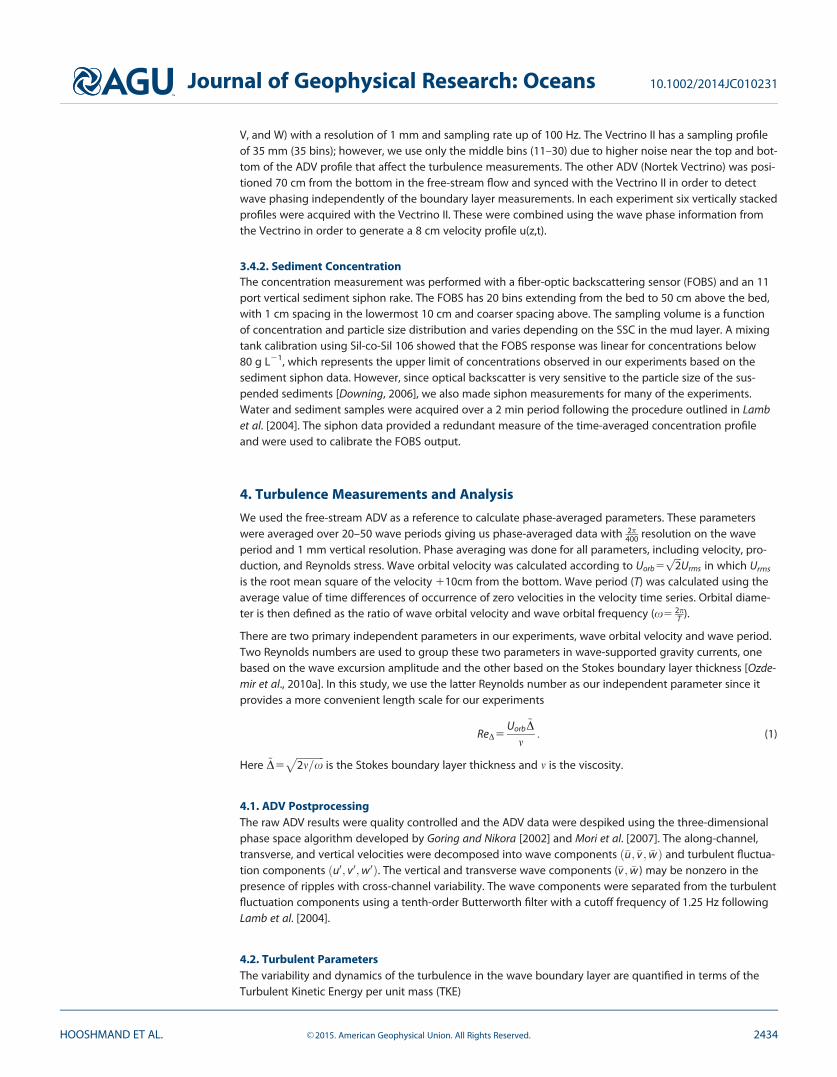
5.1. Velocity Profiles and Wave Boundary LayersThe vertical structure of the velocity profiles in oscillatory flows consists of three distinctive zones: the waveboundary layer zone (@u=@z > 0), the overshoot zone (@u=@z < 0), and the free-stream zone (@u=@z � 0)[Nielsen, 1992; Lamb et al., 2004]. These three zones are shown for the velocity profile during the maximumvelocity phase in Figure 2a. The wave boundary layer (d) is the point on the border of the wave boundarylayer and overshoot zones where the maximum velocity occurs.

The three zones are maintained through each wave phase, but the structure and shear within the boundarylayer and overshoot zones are strongly modified. The modification of the wave boundary layer structurewithin the first half wave period is shown in Figure 2b. The thickness of the wave boundary layer changes



dramatically from 0.3 to 3 cm from the beginning of the wave period until it maximum thickness at flowreversal when a new boundary layer develops. Variations in the maximum velocity and boundary layerthickness result in a peak boundary layer shear that occurs at t5 T

8.

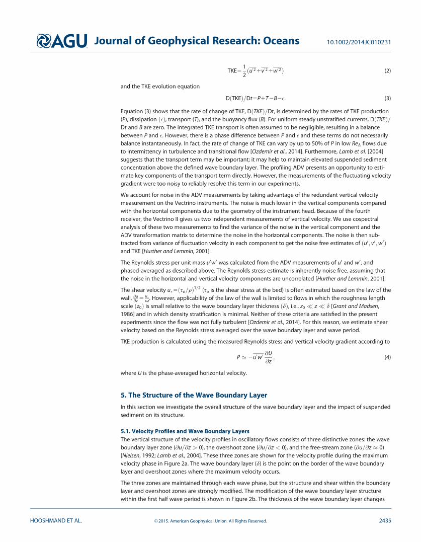
The wave boundary layer thickness d is strongly influenced by bed forms and the turbulence level. In Figure3, d, estimated based on the velocity and Reynolds stress profiles, is shown for the rough wall and sedimentbed runs. The Reynolds stress generally switches sign at the top of the boundary layer because the sign ofthe shear also changes; thus, d can also be estimated based on the zero crossing in the Reynolds stress pro-file. Wave boundary layer height scales with the ratio of shear velocity and wave frequency ðd / u�

xÞ [Hsuand Jan, 1998]. In the rough wall experiments, d increases as Uorb increases since u� increases monotonicallyas Uorb increases. This is consistent with theoretical predictions for wave boundary layer thickness [Wibergand Smith, 1983]. In Figure 3 and subsequent figures, we use ReD, defined in equation (1), as the independ-ent variable because it captures variations in Uorb and T; however, variation in ReD primarily reflect variationsin Uorb because of the stronger functional dependence on velocity and because Uorb was varied over a largerrange than T. For all but the lowest ReD, the observed boundary layer thicknesses are significantly greaterthan the analytical solution of the laminar boundary layer thickness ðdlam � 3:75

ffiffiffiffi2mx

qÞ.

The boundary layer behaves very differently in the sediment bed experiments compared with the roughwall runs (Figure 3), in part because shear velocity does not increase as Uorb increases. For low ReD, d is 2–4times greater than in the rough wall runs. As ReD increases above 400–500, however, d decreases signifi-cantly. As will be discussed later, the elevated values of d for low ReD are attributed to the presence of rip-ples in this regime and the reduction of d is attributed to increased density stratification at high ReD, inaddition to a decrease in ripple steepness. Lamb et al. [2004] and Ozdemir et al. [2010a] both observed simi-lar reductions in wave boundary layer thickness and concluded that it was due to stratification. In their DNSruns, Ozdemir et al. [2010a] further show that the boundary layer can be laminarized; however, this is notobserved in our experiments.

6. Bed Response and Sediment Profile

The addition of an active sediment bed adds two primary components to the wave boundary layer. First,the mobile bed can form ripples and bed forms that increase the roughness of the bed and modify the tur-bulence in the wave boundary layer. Second, sediment is suspended in and above the wave boundary layer,where it can modify the effective density of the fluid and exert an influence on the turbulence via densitystratification. In addition, the high-concentration suspended sediment layer that is generated by the turbu-lent flow is available to be transported due to its negative buoyancy when the bed is sloped. Here we reportthe variations in bed forms and the suspended sediment concentration profiles.

Figure 2. Velocity profiles (a) at maximum velocity phase for a rough wall experiment with Uorb545 cm s21 and T57:4 s. The velocity pro-file contains three regions: wave boundary layer, overshoot, and free stream. (b) Wave boundary layer (WBL) growth over a half phase forthe same rough wall experiment. The dashed line marks the wave boundary layer height progression and the colors represent the phasing(white corresponds to t 5 0, when the velocity is zero, and black corresponds to t5T=2, when flow reversal occurs).



6.1. Bed FormsBed forms play an important role ininitiation of sediment suspension,governing the bed shear stress andintensifying near-bed turbulence.They appear in many natural environ-ments and have different shapes andpatterns depending on the flowstructure and the particle size distri-bution of the bed. In shallow regionsof the inner continental shelf, thedominant bed forms are ripples[Hanes et al., 2001]. These ripples typ-ically have irregular two-dimensionalforms, similar to those observed inthe present laboratory experiments.A few nondimensional numbers have

been proposed to determine the criteria for existence of ripples and their steepness, wavelength, andheight.

Grant and Madsen [1982] determined ripple type based on the bed shear stress nondimensionalized by thecritical shear stress. Nielsen [1981] and Van Rijn [1993] used the mobility number defined as w5

U2orb

sgD50where

s 5 1.65 is the submerged weight of sediment relative to water and D50 is the median size for sediment par-ticles. Wiberg and Harris [1994] used near-bed orbital diameter ðd05 2Uorb

x Þ nondimensionalized by the rippleheight ðd0

g Þ where g is ripple height.

Ripples are observed in almost all of our sediment bed experiments, and their morphology changes as theflow forcing is varied. We interpret these changes following Wiberg and Harris [1994], who suggested thatripples be classified into three types based on the dimensionless orbital diameter d0=g. Here d05 2Uorb

x is theorbital diameter and g is the ripple height. According to the Wiberg and Harris’s [1994] classification scheme,orbital ripples are observed when d0=g < 20 and have wavelengths proportional to the wave orbital diame-ter. Anorbital ripples are observed when d0=g > 100 and have wavelengths proportional to the grain sizeand independent of orbital diameter. Finally, suborbital ripples are observed when 20 < d0=g < 100 andhave wavelengths that are not proportional to the orbital diameter or grain size.

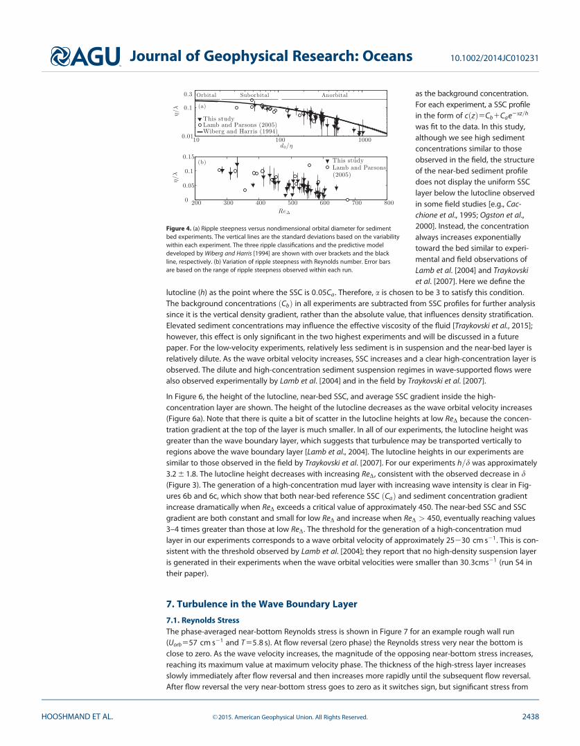
The ripple height and wavelength k in our experiments were estimated from multiple photographs takenthrough the tank wall during each experiment. The ripple steepness g=k was then calculated and averagedover the experiment period. Almost all of the ripples observed in our experiments were in the anorbitalrange (Figure 4a). The curve suggested by Wiberg and Harris [1994] captures our data relatively well; how-ever, it overestimates the ripples steepness for high d0=g. Note that while the sediment that was used inthe sediment bed runs was mostly fine silt (D50523lm), Lamb and Parsons [2005] showed that the sedimentin the ripples consist primarily of sands (D570lm) as a result of sediment bed coarsening. Lamb and Par-sons [2005] used similar sediment and the same flow facility for their experiments.

We observe that ripple steepness decreases with increasing wave forcing (ReD), consistent with the findingsof Wiberg and Harris [1994] (Figure 4b). Higher wave orbital velocities suspend more sediment and thishigher proportion of sediments in suspension is associated with a decrease in ripple steepness [Wiberg andHarris, 1994]. The range of ripple heights, from 1 to 10 mm, is well below the wave boundary layer heightðg=dw < 0:25Þ, consistent with the characterization of the bed forms as anorbital ripples; orbital rippleheights are larger than the wave boundary layer ðg=dw > 2Þ [Wiberg and Harris, 1994]. The ripple height,wavelength, and steepness observed in our experiments are in the same range as those reported in previ-ous experiments [Lamb and Parsons, 2005; Van Rijn, 2007; O’Donoghue et al., 2006; Vongvisessomjai, 1984].

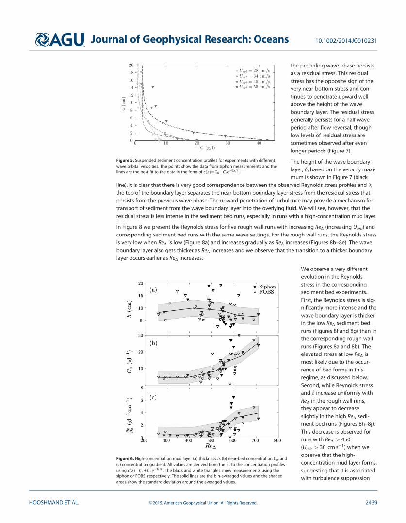
6.2. Suspended Sediment ConcentrationThe observed suspended sediment concentration (SSC) profiles for the sediment bed experiments decreaseapproximately exponentially from their peak value at the bed to a constant background value far from thebed, which is due to mixing in the end tanks (Figure 5). We designate Ca as the near-bed concentration and Cb

Figure 3. Wave boundary layer height (d) for rough wall (gray) and sediment bed(black) experiments. Squares and triangles indicate measurements of d based onthe velocity and Reynolds stress profiles, respectively, as described in the text.The thick line is the mean value. The dark gray squares and fit to those data arean estimate of the laminar boundary layer thickness for each experimentðdlaminar � 3:75~Þ, where ~D5

ffiffiffiffi2mx

qis the Stokes boundary layer thickness.



as the background concentration.For each experiment, a SSC profilein the form of cðzÞ5Cb1Cae2az=h

was fit to the data. In this study,although we see high sedimentconcentrations similar to thoseobserved in the field, the structureof the near-bed sediment profiledoes not display the uniform SSClayer below the lutocline observedin some field studies [e.g., Cac-chione et al., 1995; Ogston et al.,2000]. Instead, the concentrationalways increases exponentiallytoward the bed similar to experi-mental and field observations ofLamb et al. [2004] and Traykovskiet al. [2007]. Here we define the

lutocline (h) as the point where the SSC is 0:05Ca. Therefore, a is chosen to be 3 to satisfy this condition.The background concentrations ðCbÞ in all experiments are subtracted from SSC profiles for further analysissince it is the vertical density gradient, rather than the absolute value, that influences density stratification.Elevated sediment concentrations may influence the effective viscosity of the fluid [Traykovski et al., 2015];however, this effect is only significant in the two highest experiments and will be discussed in a futurepaper. For the low-velocity experiments, relatively less sediment is in suspension and the near-bed layer isrelatively dilute. As the wave orbital velocity increases, SSC increases and a clear high-concentration layer isobserved. The dilute and high-concentration sediment suspension regimes in wave-supported flows werealso observed experimentally by Lamb et al. [2004] and in the field by Traykovski et al. [2007].

In Figure 6, the height of the lutocline, near-bed SSC, and average SSC gradient inside the high-concentration layer are shown. The height of the lutocline decreases as the wave orbital velocity increases(Figure 6a). Note that there is quite a bit of scatter in the lutocline heights at low ReD because the concen-tration gradient at the top of the layer is much smaller. In all of our experiments, the lutocline height wasgreater than the wave boundary layer, which suggests that turbulence may be transported vertically toregions above the wave boundary layer [Lamb et al., 2004]. The lutocline heights in our experiments aresimilar to those observed in the field by Traykovski et al. [2007]. For our experiments h=d was approximately3.2 6 1.8. The lutocline height decreases with increasing ReD, consistent with the observed decrease in d(Figure 3). The generation of a high-concentration mud layer with increasing wave intensity is clear in Fig-ures 6b and 6c, which show that both near-bed reference SSC ðCaÞ and sediment concentration gradientincrease dramatically when ReD exceeds a critical value of approximately 450. The near-bed SSC and SSCgradient are both constant and small for low ReD and increase when ReD > 450, eventually reaching values3–4 times greater than those at low ReD. The threshold for the generation of a high-concentration mudlayer in our experiments corresponds to a wave orbital velocity of approximately 25230 cm s21. This is con-sistent with the threshold observed by Lamb et al. [2004]; they report that no high-density suspension layeris generated in their experiments when the wave orbital velocities were smaller than 30:3cms21 (run S4 intheir paper).

7. Turbulence in the Wave Boundary Layer

7.1. Reynolds StressThe phase-averaged near-bottom Reynolds stress is shown in Figure 7 for an example rough wall run(Uorb557 cm s21 and T55:8 s). At flow reversal (zero phase) the Reynolds stress very near the bottom isclose to zero. As the wave velocity increases, the magnitude of the opposing near-bottom stress increases,reaching its maximum value at maximum velocity phase. The thickness of the high-stress layer increasesslowly immediately after flow reversal and then increases more rapidly until the subsequent flow reversal.After flow reversal the very near-bottom stress goes to zero as it switches sign, but significant stress from

Figure 4. (a) Ripple steepness versus nondimensional orbital diameter for sedimentbed experiments. The vertical lines are the standard deviations based on the variabilitywithin each experiment. The three ripple classifications and the predictive modeldeveloped by Wiberg and Harris [1994] are shown with over brackets and the blackline, respectively. (b) Variation of ripple steepness with Reynolds number. Error barsare based on the range of ripple steepness observed within each run.



the preceding wave phase persistsas a residual stress. This residualstress has the opposite sign of thevery near-bottom stress and con-tinues to penetrate upward wellabove the height of the waveboundary layer. The residual stressgenerally persists for a half waveperiod after flow reversal, thoughlow levels of residual stress aresometimes observed after evenlonger periods (Figure 7).

The height of the wave boundarylayer, d, based on the velocity maxi-mum is shown in Figure 7 (black

line). It is clear that there is very good correspondence between the observed Reynolds stress profiles and d;the top of the boundary layer separates the near-bottom boundary layer stress from the residual stress thatpersists from the previous wave phase. The upward penetration of turbulence may provide a mechanism fortransport of sediment from the wave boundary layer into the overlying fluid. We will see, however, that theresidual stress is less intense in the sediment bed runs, especially in runs with a high-concentration mud layer.

In Figure 8 we present the Reynolds stress for five rough wall runs with increasing ReD (increasing Uorb) andcorresponding sediment bed runs with the same wave settings. For the rough wall runs, the Reynolds stressis very low when ReD is low (Figure 8a) and increases gradually as ReD increases (Figures 8b–8e). The waveboundary layer also gets thicker as ReD increases and we observe that the transition to a thicker boundarylayer occurs earlier as ReD increases.

We observe a very differentevolution in the Reynoldsstress in the correspondingsediment bed experiments.First, the Reynolds stress is sig-nificantly more intense and thewave boundary layer is thickerin the low ReD sediment bedruns (Figures 8f and 8g) than inthe corresponding rough wallruns (Figures 8a and 8b). Theelevated stress at low ReD ismost likely due to the occur-rence of bed forms in thisregime, as discussed below.Second, while Reynolds stressand d increase uniformly withReD in the rough wall runs,they appear to decreaseslightly in the high ReD sedi-ment bed runs (Figures 8h–8j).This decrease is observed forruns with ReD > 450(Uorb > 30 cm s21) when weobserve that the high-concentration mud layer forms,suggesting that it is associatedwith turbulence suppression

Figure 5. Suspended sediment concentration profiles for experiments with differentwave orbital velocities. The points show the data from siphon measurements and thelines are the best fit to the data in the form of cðzÞ5Cb1Cae23z=h .

Figure 6. High-concentration mud layer (a) thickness h, (b) near-bed concentration Ca, and(c) concentration gradient. All values are derived from the fit to the concentration profilesusing cðzÞ5Cb1Cae23z=h . The black and white triangles show measurements using thesiphon or FOBS, respectively. The solid lines are the bin-averaged values and the shadedareas show the standard deviation around the averaged values.



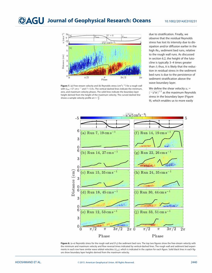
due to stratification. Finally, weobserve that the residual Reynoldsstress has lost its intensity due to dis-sipation and/or diffusion earlier in thehigh ReD sediment bed runs, relativeto the rough wall runs. As discussedin section 6.2, the height of the luto-cline is typically 3–4 times greaterthan d; thus, it is likely that the reduc-tion in residual stress in the sedimentbed runs is due to the persistence ofsediment stratification above thewave boundary layer.

We define the shear velocity u�5ð2u0wÞ1=2 as the maximum Reynoldsstress in the boundary layer (Figure9), which enables us to more easily

Figure 7. (a) Free-stream velocity and (b) Reynolds stress (cm2s22) for a rough wallwith Uorb557 cm s21 and T55:8 s. The vertical dashed lines indicate the minimum,zero, and maximum-velocity phases. The solid lines indicate the boundary layerheight derived from the height of the maximum velocity. The curved dashed lineshows a sample velocity profile at t5 3T

8 .

Figure 8. (a–e) Reynolds stress for the rough wall and (f–j) the sediment bed runs. The top two figures show the free-stream velocity withthe minimum and maximum velocity and flow reversal times indicated by vertical-dashed lines. The rough wall and sediment bed experi-ments in each row have similar wave orbital velocities (Uorb), which is indicated in the caption for each figure. Solid black lines in each fig-ure show boundary layer heights derived from the maximum velocity.



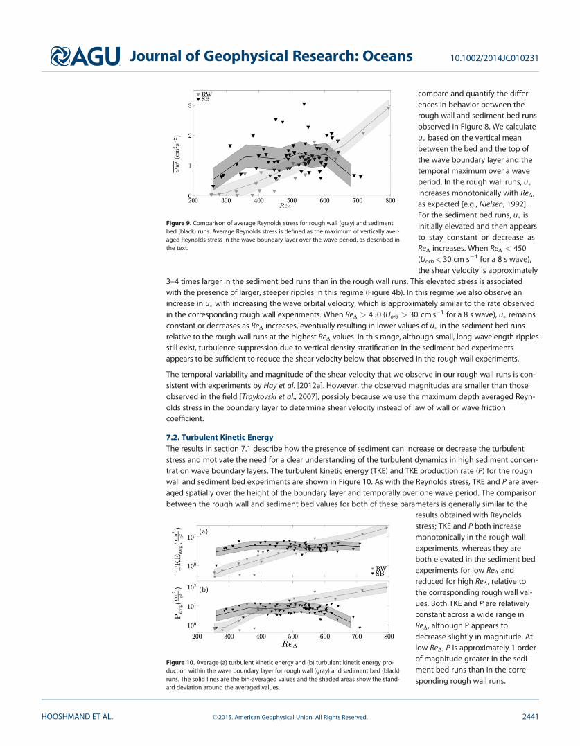
compare and quantify the differ-ences in behavior between therough wall and sediment bed runsobserved in Figure 8. We calculateu� based on the vertical meanbetween the bed and the top ofthe wave boundary layer and thetemporal maximum over a waveperiod. In the rough wall runs, u�increases monotonically with ReD,as expected [e.g., Nielsen, 1992].For the sediment bed runs, u� isinitially elevated and then appearsto stay constant or decrease asReD increases. When ReD < 450(Uorb< 30 cm s21 for a 8 s wave),the shear velocity is approximately

3–4 times larger in the sediment bed runs than in the rough wall runs. This elevated stress is associatedwith the presence of larger, steeper ripples in this regime (Figure 4b). In this regime we also observe anincrease in u� with increasing the wave orbital velocity, which is approximately similar to the rate observedin the corresponding rough wall experiments. When ReD > 450 (Uorb > 30 cm s21 for a 8 s wave), u� remainsconstant or decreases as ReD increases, eventually resulting in lower values of u� in the sediment bed runsrelative to the rough wall runs at the highest ReD values. In this range, although small, long-wavelength ripplesstill exist, turbulence suppression due to vertical density stratification in the sediment bed experimentsappears to be sufficient to reduce the shear velocity below that observed in the rough wall experiments.

The temporal variability and magnitude of the shear velocity that we observe in our rough wall runs is con-sistent with experiments by Hay et al. [2012a]. However, the observed magnitudes are smaller than thoseobserved in the field [Traykovski et al., 2007], possibly because we use the maximum depth averaged Reyn-olds stress in the boundary layer to determine shear velocity instead of law of wall or wave frictioncoefficient.

7.2. Turbulent Kinetic EnergyThe results in section 7.1 describe how the presence of sediment can increase or decrease the turbulentstress and motivate the need for a clear understanding of the turbulent dynamics in high sediment concen-tration wave boundary layers. The turbulent kinetic energy (TKE) and TKE production rate (P) for the roughwall and sediment bed experiments are shown in Figure 10. As with the Reynolds stress, TKE and P are aver-aged spatially over the height of the boundary layer and temporally over one wave period. The comparisonbetween the rough wall and sediment bed values for both of these parameters is generally similar to the

results obtained with Reynoldsstress; TKE and P both increasemonotonically in the rough wallexperiments, whereas they areboth elevated in the sediment bedexperiments for low ReD andreduced for high ReD, relative tothe corresponding rough wall val-ues. Both TKE and P are relativelyconstant across a wide range inReD, although P appears todecrease slightly in magnitude. Atlow ReD, P is approximately 1 orderof magnitude greater in the sedi-ment bed runs than in the corre-sponding rough wall runs.

Figure 9. Comparison of average Reynolds stress for rough wall (gray) and sedimentbed (black) runs. Average Reynolds stress is defined as the maximum of vertically aver-aged Reynolds stress in the wave boundary layer over the wave period, as described inthe text.

Figure 10. Average (a) turbulent kinetic energy and (b) turbulent kinetic energy pro-duction within the wave boundary layer for rough wall (gray) and sediment bed (black)runs. The solid lines are the bin-averaged values and the shaded areas show the stand-ard deviation around the averaged values.



8. Discussion

Understanding the physical detailsof wave-supported mudflows is akey step in improving our predic-tion of sediment transport acrossthe continental shelf. High-resolution measurements of thedynamics of these flows are chal-lenging in the field because theyhave relatively small vertical scalesand are very episodic in nature. Thepresent laboratory experimentssimulate the conditions underwhich wave-supported mudflowsoccur on the continental shelf anduse detailed measurements ofvelocity and turbulence with andwithout sediment to understandthe relationship between beddynamics, suspended sediment,and turbulence in the wave bound-ary layer. Our overall goal is to clar-ify the processes that determinethe vertical profiles of suspendedsediment and velocity in wave-supported mud layers in order toimprove models of cross-shelf sedi-ment transport.

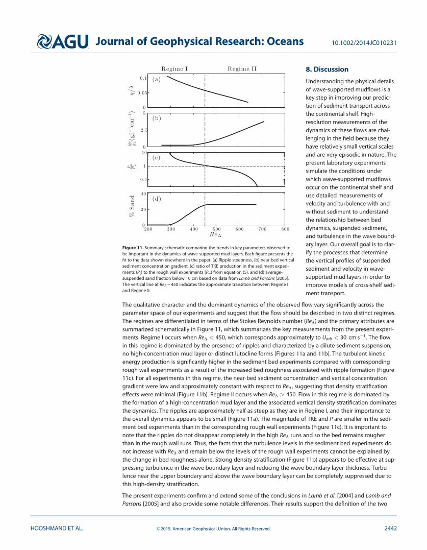
The qualitative character and the dominant dynamics of the observed flow vary significantly across theparameter space of our experiments and suggest that the flow should be described in two distinct regimes.The regimes are differentiated in terms of the Stokes Reynolds number (ReD) and the primary attributes aresummarized schematically in Figure 11, which summarizes the key measurements from the present experi-ments. Regime I occurs when ReD < 450, which corresponds approximately to Uorb < 30 cm s21. The flowin this regime is dominated by the presence of ripples and characterized by a dilute sediment suspension;no high-concentration mud layer or distinct lutocline forms (Figures 11a and 11b). The turbulent kineticenergy production is significantly higher in the sediment bed experiments compared with correspondingrough wall experiments as a result of the increased bed roughness associated with ripple formation (Figure11c). For all experiments in this regime, the near-bed sediment concentration and vertical concentrationgradient were low and approximately constant with respect to ReD, suggesting that density stratificationeffects were minimal (Figure 11b). Regime II occurs when ReD > 450. Flow in this regime is dominated bythe formation of a high-concentration mud layer and the associated vertical density stratification dominatesthe dynamics. The ripples are approximately half as steep as they are in Regime I, and their importance tothe overall dynamics appears to be small (Figure 11a). The magnitude of TKE and P are smaller in the sedi-ment bed experiments than in the corresponding rough wall experiments (Figure 11c). It is important tonote that the ripples do not disappear completely in the high ReD runs and so the bed remains rougherthan in the rough wall runs. Thus, the facts that the turbulence levels in the sediment bed experiments donot increase with ReD and remain below the levels of the rough wall experiments cannot be explained bythe change in bed roughness alone. Strong density stratification (Figure 11b) appears to be effective at sup-pressing turbulence in the wave boundary layer and reducing the wave boundary layer thickness. Turbu-lence near the upper boundary and above the wave boundary layer can be completely suppressed due tothis high-density stratification.

The present experiments confirm and extend some of the conclusions in Lamb et al. [2004] and Lamb andParsons [2005] and also provide some notable differences. Their results support the definition of the two

Figure 11. Summary schematic comparing the trends in key parameters observed tobe important in the dynamics of wave-supported mud layers. Each figure presents thefit to the data shown elsewhere in the paper. (a) Ripple steepness, (b) near-bed verticalsediment concentration gradient, (c) ratio of TKE production in the sediment experi-ments (Ps) to the rough wall experiments (Pw) from equation (5), and (d) average-suspended sand fraction below 10 cm based on data from Lamb and Parsons [2005].The vertical line at ReD5450 indicates the approximate transition between Regime Iand Regime II.



regimes described above; they alsoobserve that no high-concentrationlayer forms for low Uorb (corre-sponding to low ReD) and suggestthat density stratification is impor-tant for reducing the boundarylayer thickness in sediment bedruns with higher Uorb. Lamb andParsons [2005] describe ripple for-mation and their results, which arereplotted in Figure 4b, are consist-ent with the present results, alsoshowing that ripple steepnessdecreases for high ReD (Regime II).Lamb et al. [2004] report that turbu-lence suppression associated withdensity stratification resulted inwave boundary layers smaller than3 mm, which approaches the thick-ness expected for laminarization ofthe boundary layer. This magnitudeof boundary layer reduction wasnot observed in our experiments. Infact, while we do observe adecrease in d as stratificationincreases, d is higher in almost allof the sediment bed runs than it isin the corresponding rough wallruns. We expect that this differencein d between our results and Lamb

et al. [2004] is probably due to the increased resolution provided by the profiling ADV used in the presentstudy compared with Lamb et al.’s [2004] point-wise velocity measurements. A central conclusion in Lambet al. [2004] is that there is a large mismatch between the thickness of the mud layer and boundary layer,which requires that there is significant upward transport of turbulence from the thin energetic boundarylayer region to maintain suspension of sediment in the region above the boundary layer. We also observethat h > d, though the mismatch is only a factor of 3–4 in our observations. However, we were not able toconfirm the importance of the turbulent transport term with our measurements. Finally, Lamb and Parsons[2005] point to the important role that sorting of grains of different size may play in the dynamics of themud layer as Uorb increases. In section 8.3 we discuss the importance of the suspended sand fraction in ourobservations.

8.1. RipplesRipples were observed in most of the sediment bed experiments and appear to play an important role ingenerating turbulence, especially at low ReD. Ripples emerge in systems with an active bed load layer andthus require a minimum amount of sand on the bed [Wiberg and Harris, 1994]. Although our initial sedimentbed contained primarily silt-size particles, segregation of sand as a result of the suspension of clays and finesilts coarsened the sediment bed, resulting in a significant active bed load layer and supporting the forma-tion of ripples. This process is described in more detail in Lamb and Parsons [2005]. Ripples change the bot-tom roughness significantly, which can increase the turbulence in the wave boundary layer and theboundary layer thickness. In the present experiments steep ripples were observed in low ReD conditions. AsReD increases the ripples steepness decreases by an order of magnitude from 0.1 to 0.01. The existence ofripples can significantly change the vertical structure of the velocity field and turbulence in and outside ofthe wave boundary layer. Doering and Baryla [2002] showed that the velocity field is strongly influenced bythe presence of ripples in their experimental wave flume. They concluded that ripples can strongly

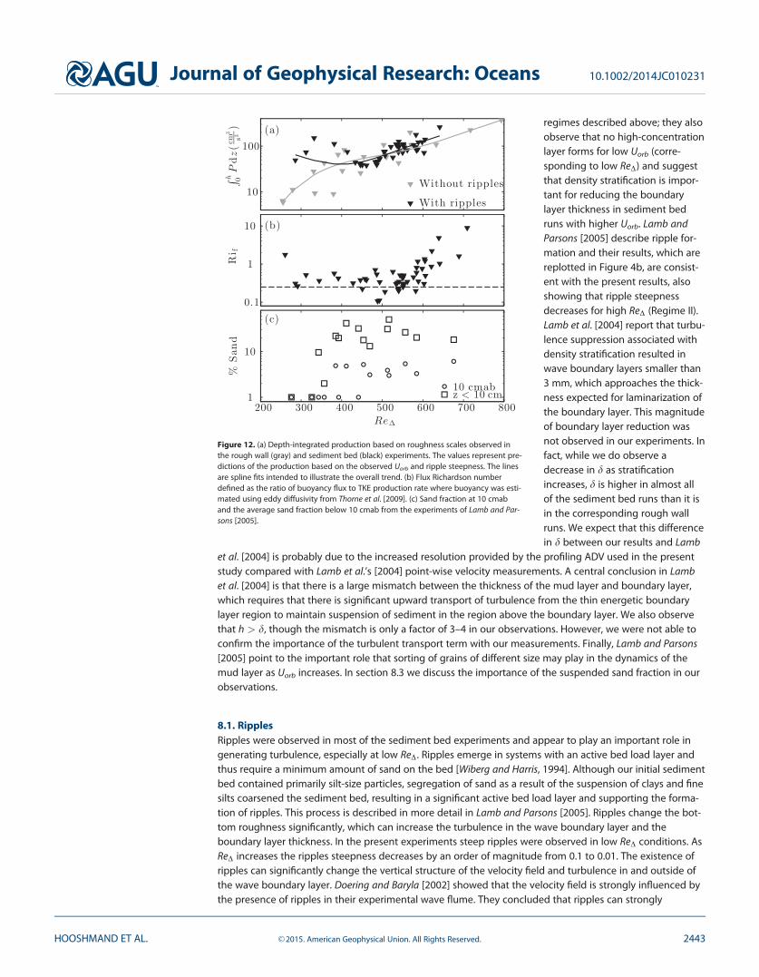
Figure 12. (a) Depth-integrated production based on roughness scales observed inthe rough wall (gray) and sediment bed (black) experiments. The values represent pre-dictions of the production based on the observed Uorb and ripple steepness. The linesare spline fits intended to illustrate the overall trend. (b) Flux Richardson numberdefined as the ratio of buoyancy flux to TKE production rate where buoyancy was esti-mated using eddy diffusivity from Thorne et al. [2009]. (c) Sand fraction at 10 cmaband the average sand fraction below 10 cmab from the experiments of Lamb and Par-sons [2005].



influence the velocity structure in a region above the ripples that is 2–4 times the ripple height. In our low ReD experiments, the observed boundary layer heights are 324cm compared with ripple heights of0:121cm. This is consistent with the upward penetration of ripple-generated turbulence observed by Doer-ing and Baryla [2002] and suggests that the enhanced thickness of the wave boundary layer in our low ReD

sediment bed experiments is a result of ripples.

We test this further by computing the predicted TKE production with and without ripples (Figure 12a) andcomparing this with our observations. The prediction uses only the observed wave orbital velocity andperiod and varies the bed roughness based on the observed ripple heights. It isolates the effect of the rip-ples on boundary layer turbulence and does not account for density stratification. The depth integratedproduction is estimated according to

Pk5bu2�Uorb; (5)

in which b is chosen to be 0.3 based on our experimental results. The shear velocity is u�5ffiffiffiffiffiffiffiffiffifw=2

pUorb, in

which the wave friction coefficient is estimated following Nielsen [1992] from

fw5exp ð5:5ðrh=AÞ0:226:3Þ; (6)

where A5Uorb=x is the wave excursion amplitude of the interior flow immediately outside the boundarylayer and rh is the hydraulics roughness of the bed. For the rough wall experiments, rh is chosen to be thesize of the sand grains on the rough bottom, D5050:75mm. These results agree qualitatively with the aver-age TKE and production measured in our experiment for ReD < 450 (Figure 10b). For the sediment bedexperiments, the observed ripple amplitudes and wavelengths were used to compute the roughness basedon rh524g2=k [Thorne et al., 2002; Hay et al., 2012b]. The predicted TKE production increases monotonicallyin rough wall experiments as expected (Figure 12a). When ripples are present, the production is significantlyhigher than in the corresponding rough wall runs, as observed in our measurements (Figure 10). This com-parison further confirms that the observed enhancement of turbulence for low ReD is due to ripples. How-ever, when ReD > 450 and the ripple steepness decreases, the predicted TKE production continues toincrease in the ripple runs and is comparable to the production in the rough wall runs (Figure 12a). This pre-diction is in contrast to the high ReD measurements, in which the production is significantly lower in thesediment bed runs than in the rough wall runs (Figure 10b). Thus, the prediction shows that productionshould increase for high ReD even though most of the ripples are washed out and another process isrequired to explain the observed suppression of turbulence. In the following section we discuss the role ofdensity stratification in suppressing turbulence in the wave boundary layer.

8.2. StratificationDensity stratification associated with high near-bed sediment concentrations can suppress turbulence inhighly stratified flows [Winterwerp, 2006]. In oscillatory boundary layers, high-density stratification maydecrease the wave boundary layer thickness and turbulence intensity. Although the turbulence level is dra-matically reduced, the turbulent energy is sufficient to maintain particle suspension in such highly stratifiedlayers primarily due to hindered settling [Winterwerp, 2006].

The numerical model results of Ozdemir et al. [2010a] suggests that turbulence suppression associated withhigh-concentration fluid muds may be sufficient to laminarize the wave boundary layer. They investigatethe effects of fine sediment on turbulence in the vicinity of the river mouths where the amount of river-borne sediment varies significantly. The wave conditions were the same for all their runs and similar to typi-cal coastal settings; the wave orbital velocity and period were 56 cm s21 and 8.6 s, respectively, resulting inReD � 1000. They performed four runs with zero, low, medium, and high sediment concentrations. In thelow-concentration runs, the near-bed sediment concentration was 10 g L21, turbulence was attenuatednear the top of the wave boundary layer due to density stratification but turbulence near the bed was unaf-fected. The maximum wave boundary layer was similar to the zero-concentration run (d52:8 cm). For themedium-concentration run, the near-bed sediment concentration was 50 g L21, turbulence was attenuatedin the entire wave boundary layer, wave boundary layer thickness was significantly reduced (d50:7cm), andthe velocity profile was very similar to that observed in a laminar flow. However, instabilities were observednear the lutocline and the flow was not completely laminarized. For the high-concentration run, the near-bed sediment concentration was 100 g L21 and the velocity structure and wave boundary layer thickness



were similar to the medium-concentration run. However, there were no instabilities and the flow was com-pletely laminarized.

The present experiments span a similar parameter range to the simulations in Ozdemir et al. [2010a] and sothey provide a good test of the model predictions. There are two important differences in the experimentalsetup; the background sediment concentration in the numerical model experiments is initially prescribedand independent of the wave settings since the model is designed to simulate direct input from rivers.However, the initial sediment conditions are identical in each of our laboratory experiments since the onlysource of suspended sediment is erosion from the bed and only the wave settings are varied. As a result,the near-bed sediment concentrations are determined entirely by the wave forcing. Also, the model runsconsist of a single grain size equivalent to a silt-sized particle. This is expected to lead to a few possible dif-ferences in the behavior of the model and experiments, most notably that no bed roughness forms in themodel.

There are a number of indications that density stratification is important in suppressing turbulence in ourexperiments. The wave boundary layer thickness decreases significantly when the flow becomes highlystratified at high ReD (Figure 3). We also observe that turbulence in upper regions of the wave boundarylayer is increasingly attenuated as stratification increases, as observed by Ozdemir et al. [2010a]. TKE and itsproduction rate in the wave boundary layer remain relatively constant and significantly lower than the cor-responding rough wall values at high ReD (Figure 10). Although the ripple steepness is significantly reducedin this regime, the bed roughness remains much higher than that in the rough wall experiments and so theturbulence intensity is expected to be as high or higher in the absence of stratification. Thus, these resultsalso suggest that density stratification is effective at suppressing turbulence, by approximately an order ofmagnitude relative to the rough wall experiments, at high ReD.

In Figure 12b, we show the flux Richardson number (Rif) results for the experiments where Rif is the ratio ofbuoyancy flux to TKE production. The buoyancy flux was estimated using a linear eddy diffusivity with theform of �s5

3ffiffi2p

10 ju�z [Thorne et al., 2009] and SSC gradients. The coefficient was chosen to take into accountthe different approaches that this study and Thorne et al. [2009] use in shear velocity estimation. Turbulentshear flows collapse when Rif exceeds a critical value Ric, where the energy required to mix sediment overthe water column is more than the available kinetic energy provided by the flow [Turner, 1973; Winterwerp,2006]. As a result, the flow becomes more stratified and cannot mix. We observe that Richardson numbersmaintain a critical value close to 1

4 for ReD < 550. This critical value is consistent with the observations ofTrowbridge and Kineke [1994] and close to 0.15, the prediction of Turner [1973] for critical flux Richardsonnumber. When ReD > 550, the flux Richardson number exceed the critical value and the flow becomesmore stratified. This region likely corresponds to the supersaturated conditions described by Winterwerp[2006] where we anticipate a collapse of the concentration profile and of the turbulent flow field.

Despite the strong turbulence suppression, we do not observe any evidence of laminarization of the flow inour data, however. TKE was always significant in the wave boundary layer, even in highly stratified conditionsand the wave boundary layer was always much thicker than what would be expected for laminar flow. Onelikely explanation for this is that there is always some roughness on the sediment bed in the experiments,whereas there is no perturbation except the initial condition in the Ozdemir et al. [2010a] simulations. Perhapsmore importantly, the sediment concentration is a result of the wave forcing in the experiments, instead of anindependent prescribed parameter. Altering wave conditions can change the concentration thresholdrequired for complete laminarization dramatically. Baas et al. [2009] showed experimentally that doubling thevelocity increased the threshold sediment concentration necessary for laminarization eightfold. Although theirexperiments were not in wavy environments, one can assume that similar trends might be applicable to waveboundary layers. Thus, we expect that the threshold for laminarization will continue to increase as the waveforcing increases, even as the near-bed sediment concentration also increases.

8.3. Transitional Behavior and the Role of Fine SandThe results summarized in Figure 11 and associated discussion indicate that the flow undergoes a transitionwhen ReD � 450; high-concentration layers can only form when ReD exceeds this threshold. It is instructiveto investigate the dynamics leading to this threshold behavior. Our results support the hypothesis that thethreshold near ReD5450 is a consequence of increases in the concentration of fine sand in suspension,which generate higher near-bed stratification, and decreases in ripple steepness.



In Figure 12c, the average sand fraction in the water column is shown based on the measurements of Lamband Parsons [2005] who performed very similar experiments in a modified version of the same facility as thepresent experiments. We show the average sand concentration 10 cmab and the average value below it.The fine sand concentration in the water column is close to zero for low ReD. Above ReD5300 the amountof sand suspended near the bed increases dramatically until it reaches close to 25% for ReD > 450. This shiftresults in a higher settling velocity and settling flux in the high-concentration layer, increasing the near-bottom stratification. Also, because turbulence is low above the boundary layer, fine sand particles are pri-marily limited to the boundary layer, further increasing the stratification, especially at the top of the layer.The intensified stratification likely suppresses turbulence, leading to a feedback that contributes to collapseof the layer thickness.

The sand dynamics may also influence the transition through their impact on ripple formation. BelowReD5450, the prevalence and influence of ripples indicates that the bed dynamics are dominated by bedload transport. Although the initial sand fraction of the bed was only approximately 10%, Lamb and Parsons[2005] show that winnowing results in sand fractions of 30–70% (their Table 1) on the bed for ReD < 450. As ReD increases above 300, more and more sand is entrained into the water column from the bed load layer. Thiscorresponds to a decrease in ripple steepness, which likely contributes to the observed transition.

It is important to note that the dynamics are probably more complicated than the description above due tothe complexity of the sediment interactions in clay-silt-sand mixtures. Even when the sediment bed consistsprimarily of sand the clay fraction can form a cohesive layer around the sand particles, resulting in signifi-cant cohesive forces [Van Rijn, 2007]. When the sediment bed mixture consists primarily of finer particles,the exact mechanism for sediment suspension is also difficult to characterize since silt particles typicallyerode as aggregates in the form of chunks rather than individual particles [Roberts and Jepsen, 1998]. Visualobservations from our experiments are consistent with this description; sediment is initially suspended inchunks, although it is likely that the chunks disaggregate after erosion.

The details of the suspension process cannot be fully resolved in our experiments. However, the observedbehavior strongly supports the conclusions that the threshold condition necessary for the generation ofhigh-concentration sediment layers is controlled largely by the character of the bed, and especially the finesand content. It follows that the threshold value of ReD, observed here to be 450, is probably a function ofsuspended sand concentration. As a result, the threshold conditions necessary for transport of sediment inwave-supported gravity currents will likely vary based on the grain size distribution in the bed deposit.

9. Summary and Conclusions

We carried out comprehensive, high-resolution measurements of velocity, turbulence, and suspended sedi-ment concentration in a wave flume in order to describe the physical processes that control the formationof wave-supported high-concentration mud layers and associated gravitational transport on the continentalshelf. Our results support the following conclusions:

1. No high-concentration sediment layer forms in Regime I, which corresponds to ReD < 450. In this regime,ripples dominate the bed dynamics, enhancing near-bed turbulence and increasing the wave boundarylayer thickness. Turbulent kinetic energy is 2–3 times higher than corresponding rough wall experimentswith similar wave conditions.

2. A high-concentration sediment layer forms in Regime II, corresponding to ReD > 450. In this regime, theripple steepness is small and the stratification due to increased fine sand content in suspension sup-presses the turbulence. Turbulent kinetic energy is lower than it is in corresponding rough wall experi-ments with similar wave conditions.

3. The flux Richardson number maintains a critical value of ’ 14 for ReD < 550 and the mud layer likely

becomes supersaturated for larger ReD values where stratification is intensified.

4. The threshold conditions that differentiate between the low and high ReD regimes appear to result fromwashout of ripples and the increase in fine sand concentration in the mud layer. The latter results in anincrease in settling flux and stratification in the high-concentration sediment layer, which may further con-tribute to the reduction in the layer thickness. However, other variables that contribute to sediment avail-ability not tested in this study are also likely to be important, such as the degree of bed consolidation.



ReferencesBaas, J. H., J. L. Best, J. Peakall, and M. Wang (2009), A phase diagram for turbulent, transitional, and laminar clay suspension flows, J. Sedi-

ment. Res., 79(4), 162–183, doi:10.2110/jsr.2009.025.Cacchione, D., D. Drake, and R. Kayen (1995), Measurements in the bottom boundary layer on the Amazon subaqueous delta, Mar. Geol.,

125(3–4), 235–257, doi:10.1016/0025-3227(95)00014-P.Colney, D. C., S. Falchetti, I. P. Lohmann, and M. Brocchini (2008), The effects of flow stratification by non-cohesive sediment on transport

in high-energy wave-driven flows, J. Fluid Mech., 610, 43–67, doi:10.1017/S0022112008002565.Doering, J., and A. J. Baryla (2002), An investigation of the velocity field under regular and irregular waves over a sand beach, Coastal Eng.,

44(4), 275–300, doi:10.1016/S0378-3839(01)00037-0.Downing, J. (2006), Twenty-five years with OBS sensors: The good, the bad, and the ugly, Cont. Shelf Res., 26(17–18), 2299–2318, doi:

10.1016/j.csr.2006.07.018.Falcini, F., S. Fagherazzi, and D. Jerolmack (2012), Wave-supported sediment gravity flows currents: Effects of fluid-induced pressure gra-

dients and flow width spreading, Cont. Shelf Res., 33, 37–50, doi:10.1016/j.csr.2011.11.004.Geyer, W. R., P. Hill, T. Milligan, and P. Traykovski (2000), The structure of the Eel River plume during floods, Cont. Shelf Res., 20, 2067–2093,

doi:10.1016/S0278-4343(00)00063-7.Goring, D., and V. Nikora (2002), Despiking acoustic Doppler velocimeter data, J. Hydraul. Eng., 128, 117–126, doi:10.1061/(ASCE)0733-

9429(2002).Grant, W. D., and O. S. Madsen (1982), Movable bed roughness in unsteady oscillatory flow, J. Geophys. Res., 87(C1), 469–481, doi:10.1029/

JC087iC01p00469.Grant, W. D., and O. Madsen (1986), The continental-shelf bottom boundary layer, Annu. Rev. Fluid Mech., 18, 265–305, doi:10.1146/

annurev.fl.18.010186.001405.Hale, R., A. S. Ogston, J. Walsh, and A. R. Orpin (2014), Sediment transport and event deposition on the Waipaoa River Shelf, New Zealand,

Cont. Shelf Res., 86, 52–65, doi:10.1016/j.csr.2014.01.009.Hamblin, A. P., and R. G. Walker (1979), Storm-dominated shallow marine deposits: The Fernie-Kootenay (Jurassic) transition, southern

Rocky Mountains, Can. J. Earth Sci., 16(9), 1673–1690, doi:10.1139/e79-156.Hanes, D. M., V. Alymov, and Y. S. Chang (2001), Wave-formed sand ripples at Duck, North Carolina, J. Geophys. Res., 106(C10), 22,575–

22,592, doi:10.1029/2000JC000337.Hare, J., A. Hay, L. Zedel, and R. Cheel (2014), Observations of the spacetime structure of flow, turbulence, and stress over orbitalscale rip-

ples, J. Geophys. Res. Oceans, 119, 1876–1898, doi:10.1002/2013JC009370.Hay, A. E., L. Zedel, R. Cheel, and J. Dillon (2012a), Observations of the vertical structure of turbulent oscillatory boundary layers above fixed

roughness using a prototype wideband coherent Doppler profiler: 2. Turbulence and stress, J. Geophys. Res., 117, C03006, doi:10.1029/2011JC007114.

Hay, A. E., L. Zedel, R. Cheel, and J. Dillon (2012b), On the vertical and temporal structure of flow and stress within the turbulent oscillatoryboundary layer above evolving sand ripples, Cont. Shelf Res., 46, 31–49, doi:10.1016/j.csr.2012.02.009.

Hsu, T., and C.-D. Jan (1998), Calibration of Businger-Arya type of eddy viscosity model’s parameters, J. Waterw. Port Coastal Ocean Eng.,124(5), 281–284.

Hsu, T.-J., C. E. Ozdemir, and P. A. Traykovski (2009), High-resolution numerical modeling of wave-supported gravity-driven mudflows, J.Geophys. Res., 114, C05014, doi:10.1029/2008JC005006.

Hurther, D., and U. Lemmin (2001), A correction method for turbulence measurements with a 3D acoustic Doppler velocity profiler, J.Atmos. Oceanic Technol., 18(3), 446–458.

Jaramillo, S., A. Sheremet, M. A. Allison, A. H. Reed, and K. T. Holland (2009), Wave-mud interactions over the muddy Atchafalaya subaqu-eous clinoform, Louisiana, United States: Wave-supported sediment transport, J. Geophys. Res., 114, C04002, doi:10.1029/2008JC004821.

Kineke, G., K. Woolfe, S. Kuehl, J. Milliman, T. Dellapenna, and R. Purdon (2000), Sediment export from the Sepik River, Papua New Guinea:Evidence for a divergent sediment plume, Cont. Shelf Res., 20(16), 2239–2266, doi:10.1016/S0278-4343(00)00069-8.

Lamb, M. P., and J. D. Parsons (2005), High-density suspensions formed under waves, J. Sediment. Res., 75(3), 386–397, doi:10.2110/jsr.2005.030.

Lamb, M. P., E. D. Asaro, and J. D. Parons (2004), Turbulent structure of high-density suspensions formed under waves, J. Geophys. Res., 109,C12026, doi:10.1029/2004JC002355.

Liang, H., M. P. Lamb, and J. D. Parsons (2007), Formation of a sandy near-bed transport layer from a fine-grained bed under oscillatoryflow, J. Geophys. Res., 112, C02008, doi:10.1029/2006JC003635.

Ma, Y., L. D. Wright, and C. T. Friedrichs (2008), Observations of sediment transport on the continental shelf off the mouth of theWaiapu River, New Zealand: Evidence for current-supported gravity flows, Cont. Shelf Res., 28(4–5), 516–532, doi:10.1016/j.csr.2007.11.001.

McPhee-Shaw, E. E., D. A. Siegel, L. Washburn, M. A. Brzezinski, J. L. Jones, A. Leydecker, and J. Melack (2007), Mechanisms for nutrient deliv-ery to the inner shelf: Observations from the Santa Barbara Channel, Limnol. Oceanogr., 52(5), 1748–1766, doi:10.4319/lo.2007.52.5.1748.

Milliman, J., and R. Meade (1983), World-wide delivery of river sediment to the oceans, J. Geol., 91(1), 1–21.Mori, N., M. Asce, T. Suzuki, and S. Kakuno (2007), Noise of acoustic Doppler velocimeter data in bubbly flows, J. Eng. Mech., 133(1), 122–

125.Nielsen, P. (1981), Dynamics and geometry of wave-generated ripples, J. Geophys. Res., 86(C7), 6467–6472.Nielsen, P. (1992), Coastal bottom boundary layers and sediment transport, Adv. Ser. Ocean Eng., World Scientific, Singapore, River Edge,

N. J. [Available at http://trove.nla.gov.au/work/20017061?selectedversion=NBD9311281.]Nittrouer, C. A. (1999), STRATAFORM: Overview of its design and synthesis of its results, Mar. Geol., 154(1–4), 3–12, doi:10.1016/S0025-

3227(98)00128-5.Nittrouer, C. A., and L. D. Wright (1994), Transport of particles across continental shelves, Rev. Geophys., 32(1), 85–113, doi:10.1029/

93RG02603.O’Donoghue, T., J. Doucette, J. van der Werf, and J. Ribberink (2006), The dimensions of sand ripples in full-scale oscillatory flows, Coastal

Eng., 53(12), 997–1012, doi:10.1016/j.coastaleng.2006.06.008.Ogston, A., and R. Sternberg (1999), Sediment-transport events on the northern California continental shelf, Mar. Geol., 154(1–4), 69–82,

doi:10.1016/S0025-3227(98)00104-2.

AcknowledgmentsWe would like to thank ChrisChickadel, Jim Riley, JPaul Rinehimer,Charles Nittrouer, and Andrea Ogstonfor support and helpful discussions,Peter Rusello and Judah Goldbergfrom Nortek for their technicalsupport, and Jeffrey Parsons forinitiating the work more than a decadeago and for his support during theproject. This research was funded bythe National Science Foundation (OCE-000488762). Data from this paper areavailable upon request. Please contactAlexander Horner-Devine([email protected]).



http://dx.doi.org/10.2110/jsr.2009.025

http://dx.doi.org/10.1016/0025-3227(95)00014-P

http://dx.doi.org/10.1017/S0022112008002565

http://dx.doi.org/10.1016/S0378-3839(01)00037-0

http://dx.doi.org/10.1016/j.csr.2006.07.018


http://dx.doi.org/10.1016/S0278-4343(00)00063-7

http://dx.doi.org/10.1061/(ASCE)0733-9429(2002)

http://dx.doi.org/10.1061/(ASCE)0733-9429(2002)

http://dx.doi.org/10.1029/JC087iC01p00469

http://dx.doi.org/10.1029/JC087iC01p00469

http://dx.doi.org/10.1146/annurev.fl.18.010186.001405

http://dx.doi.org/10.1146/annurev.fl.18.010186.001405


http://dx.doi.org/10.1139/e79-156

http://dx.doi.org/10.1029/2000JC000337

http://dx.doi.org/10.1002/2013JC009370

http://dx.doi.org/10.1029/2011JC007114

http://dx.doi.org/10.1029/2011JC007114


http://dx.doi.org/10.1029/2008JC005006

http://dx.doi.org/10.1029/2008JC004821

http://dx.doi.org/10.1029/2008JC004821

http://dx.doi.org/10.1016/S0278-4343(00)00069-8



http://dx.doi.org/10.1029/2004JC002355

http://dx.doi.org/10.1029/2006JC003635



http://dx.doi.org/10.4319/lo.2007.52.5.1748

http://dx.doi.org/10.4319/lo.2007.52.5.1748

http://trove.nla.gov.au/work/20017061?selectedversion=NBD9311281

http://dx.doi.org/10.1016/S0025-3227(98)00128-5

http://dx.doi.org/10.1016/S0025-3227(98)00128-5

http://dx.doi.org/10.1029/93RG02603

http://dx.doi.org/10.1029/93RG02603

http://dx.doi.org/10.1016/j.coastaleng.2006.06.008

http://dx.doi.org/10.1016/S0025-3227(98)00104-2

Ogston, A., D. Cacchione, R. Sternberg, and G. Kineke (2000), Observations of storm and river flood-driven sediment transport on the north-ern California continental shelf, Cont. Shelf Res., 20(16), 2141–2162, doi:10.1016/S0278-4343(00)00065-0.

Ozdemir, C. E., T.-J. Hsu, and S. Balachandar (2010a), A numerical investigation of fine particle laden flow in an oscillatory channel: The roleof particle-induced density stratification, J. Fluid Mech., 665, 1–45, doi:10.1017/S0022112010003769.

Ozdemir, C. E., T.-J. Hsu, and S. Balachandar (2010b), Simulation of fine sediment transport in oscillatory boundary layer, J. Hydro-environ.Res., 3(4), 247–259, doi:10.1016/j.jher.2009.10.013.

Ozdemir, C. E., T.-J. Hsu, and S. Balachandar (2011), A numerical investigation of lutocline dynamics and saturation of fine sediment in theoscillatory boundary layer, J. Geophys. Res., 116, C09012, doi:10.1029/2011JC007185.

Ozdemir, C. E., T.-J. Hsu, and S. Balachandar (2014), Direct numerical simulations of transition and turbulence in smooth-walled Stokesboundary layer, Phys. Fluids, 26(4), 045108, doi:10.1063/1.4871020.

Parsons, J., J. Bush, and J. Syvitski (2001), Hyperpycnal plume formation from riverine outflows with small sediment concentrations, Sedi-mentology, 48(2), 465–478, doi:10.1046/j.1365-3091.2001.00384.x.

Puig, P., A. Ogston, B. Mullenbach, C. Nittrouer, and R. Sternberg (2003), Shelf-to-canyon sediment-transport processes on the Eel continen-tal margin (northern California), Mar. Geol., 193(1–2), 129–149, doi:10.1016/S0025-3227(02)00641-2.

Roberts, J., and R. Jepsen (1998), Effects of particle size and bulk density on erosion of quartz particles, J. Hydraul. Eng., 124(12), 1261–1267.Safak, I., M. Allison, and A. Sheremet (2013), Floc variability under changing turbulent stresses and sediment availability on a wave ener-

getic muddy shelf, Cont. Shelf Res., 53, 1–10, doi:10.1016/j.csr.2012.11.015.Scully, M., C. Friedrichs, and L. Wright (2002), Application of an analytical model of critically stratified gravity-driven sediment transport

and deposition to observations from the Eel River continental shelf, Northern California, Cont. Shelf Res., 22(14), 1951–1974, doi:10.1016/S0278-4343(02)00047-X.

Sternberg, R., and D. Cacchione (1996), Observations of sediment transport on the Amazon subaqueous delta, Cont. Shelf Res., 16(5), 697–715, doi:10.1016/0278-4343(95)00045-3.

Thorne, P., J. Williams, and A. Davies (2002), Suspended sediments under waves measured in a large-scale flume facility, J. Geophys. Res.,107(C8), doi:10.1029/2001JC000988.

Thorne, P. D., A. G. Davies, and P. S. Bell (2009), Observations and analysis of sediment diffusivity profiles over sandy rippled beds underwaves, J. Geophys. Res., 114, C02023, doi:10.1029/2008JC004944.

Traykovski, P., W. Geyer, J. Irish, and J. Lynch (2000), The role of wave-induced density-driven fluid mud flows for cross-shelf transport onthe Eel River continental shelf, Cont. Shelf Res., 20(16), 2113–2140, doi:10.1016/S0278-4343(00)00071-6.

Traykovski, P., P. Wiberg, and W. Geyer (2007), Observations and modeling of wave-supported sediment gravity flows on the Po prodeltaand comparison to prior observations from the Eel shelf, Cont. Shelf Res., 27(3–4), 375–399, doi:10.1016/j.csr.2005.07.008.

Traykovski, P., J. Trowbridge, and G. Kineke (2015), Mechanisms of surface wave energy dissipation over a high-concentration sedimentsuspension, J. Geophys. Res. Oceans, 120, 1638–1681, doi:10.1002/2014JC010245.

Trowbridge, J. H., and G. C. Kineke (1994), Structure and dynamics of fluid muds on the Amazon, J. Geophys. Res., 99(C1), 865–874, doi:10.1029/93JC02860.

Turner, J. (1973), Buoyancy Effects in Fluids, 368 p., Cambridge Univ. Press, N. Y.Van Rijn, L. (1993), Principles of Sediment Transport in Rivers, Estuaries and Coastal Seas, Aqua Publ., Amsterdam, Netherlands.Van Rijn, L. (2007), Unified view of sediment transport by currents and waves. II: Suspended transport, J. Hydraul. Eng., 133(6), 668–689.Vongvisessomjai, S. (1984), Oscillatory ripple geometry, J. Hydraul. Eng., 110(3), 247–266, doi:10.1061/(ASCE)0733-9429(1984)110:3(247).Walsh, J., C. Nittrouer, C. Palinkas, A. S. Ogston, R. Sternberg, and G. Brunskill (2004), Clinoform mechanics in the Gulf of Papua, New

Guinea, Cont. Shelf Res., 24(19), 2487–2510, doi:10.1016/j.csr.2004.07.019.Wheatcroft, R. A., A. W. Stevens, and R. V. Johnson (2007), In situ time-series measurements of subseafloor sediment properties, IEEE J. Oce-

anic Eng., 32(4), 862–871, doi:10.1109/JOE.2007.907927.Wiberg, P., and J. D. Smith (1983), A comparison of field data and theoretical models for wave-current interactions at the bed on the conti-

nental shelf, Cont. Shelf Res., 2(2–3), 147–162, doi:10.1016/0278-4343(83)90013-4.Wiberg, P. L., and C. K. Harris (1994), Ripple geometry in wave-dominated environments, J. Geophys. Res., 99(C1), 775–789, doi:10.1029/

93JC02726.Winterwerp, J. C. (2006), Stratification effects by fine suspended sediment at low, medium, and very high concentrations, J. Geophys. Res.,

111, C05012, doi:10.1029/2005JC003019.Wright, L., and C. Friedrichs (2006), Gravity-driven sediment transport on continental shelves: A status report, Cont. Shelf Res., 26(17–18),

2092–2107, doi:10.1016/j.csr.2006.07.008.Wright, L., C. Sherwood, and R. Sternberg (1997), Field measurements of fairweather bottom boundary layer processes and sediment sus-

pension on the Louisiana inner continental shelf, Mar. Geol., 140(3), 329–345, doi:10.1016/S0025-3227(97)00032-7.Wright, L., S.-C. Kim, and C. Friedrichs (1999), Across-shelf variations in bed roughness, bed stress and sediment suspension on the north-

ern California shelf, Mar. Geol., 154(1–4), 99–115, doi:10.1016/S0025-3227(98)00106-6.Wright, L., C. Friedrichs, S. Kim, and M. Scully (2001), Effects of ambient currents and waves on gravity-driven sediment transport on conti-

nental shelves, Mar. Geol., 175(1–4), 25–45, doi:10.1016/S0025-3227(01)00140-2.Yan, B., Q. Zhang, and M. Lamb (2010), Time-averaged turbulent mixing and vertical concentration distribution of high-density suspensions

formed under waves, Coastal Eng., 32, 1–8.



http://dx.doi.org/10.1016/S0278-4343(00)00065-0

http://dx.doi.org/10.1017/S0022112010003769

http://dx.doi.org/10.1016/j.jher.2009.10.013

http://dx.doi.org/10.1029/2011JC007185

http://dx.doi.org/10.1063/1.4871020

http://dx.doi.org/10.1046/j.1365-3091.2001.00384.x

http://dx.doi.org/10.1016/S0025-3227(02)00641-2


http://dx.doi.org/10.1016/S0278-4343(02)00047-X

http://dx.doi.org/10.1016/0278-4343(95)00045-3

http://dx.doi.org/10.1029/2001JC000988

http://dx.doi.org/10.1029/2008JC004944

http://dx.doi.org/10.1016/S0278-4343(00)00071-6


http://dx.doi.org/10.1002/2014JC010245

http://dx.doi.org/10.1029/93JC02860

http://dx.doi.org/10.1061/(ASCE)0733-9429(1984)110:3(247)


http://dx.doi.org/10.1109/JOE.2007.907927

http://dx.doi.org/10.1016/0278-4343(83)90013-4



http://dx.doi.org/10.1029/2005JC003019


http://dx.doi.org/10.1016/S0025-3227(97)00032-7

http://dx.doi.org/10.1016/S0025-3227(98)00106-6

http://dx.doi.org/10.1016/S0025-3227(01)00140-2

Documents

Structure of turbulence and sediment stratification in