Structured low-rank approximation and its applications

Automatica 44 (2008) 891–909www.elsevier.com/locate/automatica

Survey paper

Structured low-rank approximation and its applications�

Ivan MarkovskySchool of Electronics and Computer Science, University of Southampton, SO17 1BJ, UK

Received 7 November 2006; received in revised form 2 August 2007; accepted 5 September 2007Available online 26 December 2007

Abstract

Fitting data by a bounded complexity linear model is equivalent to low-rank approximation of a matrix constructed from the data. The datamatrix being Hankel structured is equivalent to the existence of a linear time-invariant system that fits the data and the rank constraint isrelated to a bound on the model complexity. In the special case of fitting by a static model, the data matrix and its low-rank approximationare unstructured.

We outline applications in system theory (approximate realization, model reduction, output error, and errors-in-variables identification),signal processing (harmonic retrieval, sum-of-damped exponentials, and finite impulse response modeling), and computer algebra (approximatecommon divisor). Algorithms based on heuristics and local optimization methods are presented. Generalizations of the low-rank approximationproblem result from different approximation criteria (e.g., weighted norm) and constraints on the data matrix (e.g., nonnegativity). Relatedproblems are rank minimization and structured pseudospectra.� 2007 Elsevier Ltd. All rights reserved.

Keywords: Low-rank approximation; Total least squares; System identification; Errors-in-variables modeling; Behaviors

1. Introduction

Fitting linear models to data can be achieved, both concep-tually and algorithmically, by solving a system of equationsAX = B, where the matrices A and B are constructed fromthe given data and the matrix X parameterizes the model to befound. In this classical approach, the main tools are the leastsquares method and its variations—data least squares (Degroat& Dowling, 1991), total least squares (TLS) (Golub & VanLoan, 1980), structured TLS (De Moor, 1993), robust leastsquares (Chandrasekaran, Gu, & Sayed, 1998), etc. The leastsquares method and its variations are mainly motivated by theirapplications for data fitting, but they invariably consider solv-ing approximately an overdetermined system of equations.

In this paper we show that a number of linear data fittingproblems are equivalent to the abstract problem of approxi-mating a matrix D constructed from the data by a low-rank

� This paper was not presented at any IFAC meeting. This paper wasrecommended for publication in revised form by Associate Editor WolfgangScherrer under the direction of Editor Manfred Morari.

E-mail address: [email protected].

0005-1098/$ - see front matter � 2007 Elsevier Ltd. All rights reserved.doi:10.1016/j.automatica.2007.09.011

matrix. Partitioning the data matrix into matrices A ∈ RN×m

and B ∈ RN×p and solving approximately the system AX =B

is a way to achieve rank-m or less approximation. The converseimplication, however, is not true, because [A B] having rank-mor less does not imply the existence of X, such that AX = B.This lack of equivalence between the original low-rank ap-proximation problem and the AX =B problem motivates whatis called nongeneric TLS problem (Van Huffel & Vandewalle,1991), whose theory is more complicated than the one of thegeneric problem and is difficult to solve numerically.

Alternative approaches for achieving a low-rank approxima-tion are to impose that the data matrix has

1. at least p := coldim(B) dimensional nullspace, or2. at most m := coldim(A) dimensional column space.

Parameterizing the nullspace and the column space by sets ofbasis vectors, the alternative approaches are:

1. kernel representation: there is a full rank matrix R ∈Rp×(m+p), such that [A B]R� = 0, and

2. image representation: there are matrices P ∈ R(m+p)×m andL ∈ Rm×N , such that [A B]� = PL.

http://www.elsevier.com/locate/automatica

mailto:[email protected]

892 I. Markovsky / Automatica 44 (2008) 891–909

The approaches using kernel and image representations areequivalent to the original low-rank approximation problem.Next we illustrate the use of AX =B, kernel, and image repre-sentations on the most simple data fitting problem—line fitting.

1.1. Line fitting example

Given a set of points { d1, . . . , dN } ⊂ R2 in the plane, theaim of the line fitting problem is to find a line passing throughthe origin that “best” matches the given points. The classicalapproach for line fitting is to define col(ai, bi) := di and solveapproximately the overdetermined system

col(a1, . . . , aN)x = col(b1, . . . , bN) (1)

by the least squares method. Let xls be the least squaresapproximate solution to (1). Then the least squares fitting line is

Bls := {d = col(a, b) ∈ R2 | axls = b}. (2)

Geometrically, Bls minimizes the sum of the squared verticaldistances from the data points to the fitting line.

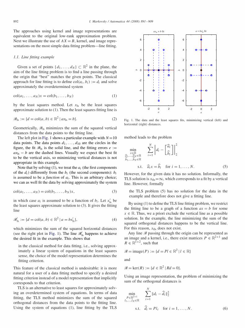
The left plot in Fig. 1 shows a particular example with N=10data points. The data points d1, . . . , d10 are the circles in thefigure, the fit Bls is the solid line, and the fitting errors e :=axls − b are the dashed lines. Visually we expect the best fitto be the vertical axis, so minimizing vertical distances is notappropriate in this example.

Note that by solving (1), we treat the ai (the first componentsof the di) differently from the bi (the second components): bi

is assumed to be a function of ai . This is an arbitrary choice;we can as well fit the data by solving approximately the system

col(a1, . . . , aN) = col(b1, . . . , bN)x, (3)

in which case ai is assumed to be a function of bi . Let x′ls be

the least squares approximate solution to (3). It gives the fittingline

B′ls := {d = col(a, b) ∈ R2 | a = bx′

ls}, (4)

which minimizes the sum of the squared horizontal distances(see the right plot in Fig. 1). The line B′

ls happens to achievethe desired fit in the example. This shows that

in the classical method for data fitting, i.e., solving approx-imately a linear system of equations in the least squaressense, the choice of the model representation determines thefitting criterion.

This feature of the classical method is undesirable: it is morenatural for a user of a data fitting method to specify a desiredfitting criterion instead of a model representation that implicitlycorresponds to that criterion.

TLS is an alternative to least squares for approximately solv-ing an overdetermined system of equations. In terms of datafitting, the TLS method minimizes the sum of the squaredorthogonal distances from the data points to the fitting line.Using the system of equations (1), line fitting by the TLS

-2 0 2

-6

-4

-2

0

2

4

6

a

b

axls = b fit

-2 0 2

-6

-4

-2

0

2

4

6

a

b

a = bxls fit′

Fig. 1. The data and the least squares fits, minimizing vertical (left) andhorizontal (right) distances.

method leads to the problem

minx∈R

a1,...,aN∈Rb1,...,bN∈R

N∑i=1

∥∥∥∥di −[ai

bi

]∥∥∥∥2

2

s.t. aix = bi for i = 1, . . . , N. (5)

However, for the given data it has no solution. Informally, theTLS solution is xtls=∞, which corresponds to a fit by a verticalline. However, formally

the TLS problem (5) has no solution for the data in theexample and therefore does not give a fitting line.

By using (1) to define the TLS line fitting problem, we restrictthe fitting line to be a graph of a function ax = b for somex ∈ R. Thus, we a priori exclude the vertical line as a possiblesolution. In the example, the line minimizing the sum of thesquared orthogonal distances happens to be the vertical line.For this reason, xtls does not exist.

Any line B passing through the origin can be represented asan image and a kernel, i.e., there exist matrices P ∈ R2×1 andR ∈ R1×2, such that

B = image(P ) := {d = Pl ∈ R2 | l ∈ R}and

B = ker(R) := {d ∈ R2 | Rd = 0}.Using an image representation, the problem of minimizing thesum of the orthogonal distances is

minP∈R2×1

l1,...,lN∈R

N∑i=1

‖di − di‖22

s.t. di = P li for i = 1, . . . , N . (6)

I. Markovsky / Automatica 44 (2008) 891–909 893

With D := [d1 · · · dN ], D := [d1 · · · dN ], and ‖·‖F theFrobenius norm, (6) is more compactly written as

minP∈R2×1

L∈R1×N

‖D − D‖2F

s.t. D = PL. (7)

Similarly, using a kernel representation, we have

minR∈R1×2,R �=0

D∈R2×N

‖D − D‖2F

s.t. RD = 0. (8)

Contrary to the TLS problem (5), problems (7) and (8) alwayshave (possibly nonunique) solutions. In the example, solutionsare, e.g., P ∗ = col(0, 1) and R∗ = [1 0], which describe thevertical line B∗ := image(P ∗) = ker(R∗).

The constraints D=PL, P ∈ R2×1, L ∈ R1×N , and RD=0,R ∈ R1×2, R �= 0 are equivalent to the constraint rank(D)�1,which shows that the points

{d1, . . . , dN } being fitted exactly by a line passing throughthe origin is equivalent to rank([d1 · · · dN ])�1.

In fact, (7) and (8) are instances of one and the same ab-stract problem: approximate the data matrix D by a rank-onematrix D.

1.2. Input/output interpretation of AX = B

The underlying goal is: given a set of points in Rd, find asubspace of Rd of bounded dimension that has the least 2-normdistance to all points. Such a subspace is an optimal (in the2-norm sense) fitting model. The most general way to repre-sent any subspace in Rd is the kernel or image formulation;the classical least squares and TLS formulations exclude somesubspaces. As illustrated by the example, the equations ax = b

and a = bx, used in the least squares and TLS problem for-mulations to represent the subspace, might fail to represent theoptimal solution, while the kernel and image representationsdo not have such deficiency. This suggests that the kernel andimage representations are better suited for data fitting.

The equations ax=b and a=bx were introduced from an algo-rithmic point of view—by using them, the data fitting problemis turned into the standard problem of solving approximatelyan overdetermined system of equations. There is another, moreinsightful, interpretation of these equations that comes fromsystem theory. In the model represented by the equation ax=b,the variable a is an input, meaning that it is free, and the vari-able b is an output, meaning that it is bound by the input andthe model. Similarly, in the model represented by the equationa = bx, the variable a is an output and the variable b is an in-put. The input/output interpretation has an intuitive appeal be-cause it shows a causal dependence of the variables: the inputis causing the output.

Representing the model by an equation ax = b or a = bx,as done in the classical method, one a priori assumes that the

optimal fitting model has a certain input/output structure. Theconsequences are:

• existence of exceptional (nongeneric) cases, which compli-cate the theory,

• ill-conditioning caused by “nearly” exceptional cases, whichleads to lack of numerical robustness of the algorithms, and

• need of regularization, which leads to a change of the spec-ified fitting criterion.

These aspects of the classical method are generally consideredas inherent to the data fitting problem. In fact, by choosing thealternative image and kernel model representations the non-generic problems (and the related issues of ill-conditioning andneed of regularization) are avoided.

1.3. Contributions of the paper and related work

Connections between data modeling problems and low-rankapproximation—the topic of this paper—abound in the litera-ture; however, often they are implicit and not deemed essential.The following are examples where the fact that an exact (noise-free) data matrix is low-rank is a common knowledge and isexploited in solution methods:

• realization theory—a sequence

H = (H(0), H(1), . . . , H(t), . . .)

is an impulse response of a linear time-invariant (LTI) systemof order n if and only if the (infinite) Hankel matrix

H(H) :=

⎡⎢⎢⎢⎢⎢⎣

H(1) H(2) H(3) · · ·H(2) H(3) T

H(3) T...

⎤⎥⎥⎥⎥⎥⎦

constructed from H has rank n;• direction-of-arrival problem in signal processing—the rank

of an exact data matrix equals the number of sources;• chemometrics—the rank of an exact data matrix equals the

number of chemical components.

Although omnipresent, however, until now the structured low-rank approximation (SLRA) problem has not been generallyperceived as a data modeling principle. It is the belief of theauthor that

behind every linear data modeling problem there is a (hid-den) low-rank approximation problem: the model imposesrelations on the data which render a matrix constructed fromexact data rank deficient.

Low-rank approximation is used in a number of data model-ing problems from diverse scientific fields; however, there areproblems, e.g., frequency domain and stochastic system iden-tification, that are still awaiting for such an interpretation.


De Moor (1993, 1994), defines a generic problem, calledstructured TLS, and shows a number of applications that reduceto it. The structured TLS problem corresponds to the SLRAproblem, defined in this paper (see Section 2.2) when a ker-nel representation is used to represent the rank constraint. Weconsider the more general SLRA problem because it gives free-dom in choosing different representations for solving particularproblems.

The rank constraint in the low-rank approximation problemcorresponds to the constraint that the data are fitted by a lin-ear model of bounded complexity in the data fitting problem.Therefore, the question of representing the rank constraint in thelow-rank approximation problem corresponds to the questionof choosing the model representation in the data fitting prob-lem. The behavioral approach to system theory put forward byWillems (1986, 1987) is a manifestation of the representationfree thinking. Deriving dynamic models from data, i.e., sys-tem identification, has been considered in the behavioral settingin Roorda and Heij (1995), Roorda (1995), and Markovsky,Willems, Van Huffel, De Moor, and Pintelon (2005).

The contributions of this paper are:

1. embed the structured TLS problem in the behavioral setting,2. complete the list of applications in De Moor (1993) with out-

put error identification, pole placement, harmonic retrieval,and approximate common divisor problems,

3. present generalizations and connections of the structuredTLS problem to problems with nonnegativity constraint,rank minimization, and structured pseudospectra, and

4. give a tutorial to a representative set of data modeling prob-lems from a unifying viewpoint.

1.4. Outline of the paper

Section 2 defines the low-rank approximation problem as arepresentation free data modeling problem, applying to gen-eral multivariable static and dynamic problems. Approximationby an unstructured matrix corresponds to fitting the data by astatic linear model. Approximation by a Hankel structured ma-trix corresponds to fitting the data by a dynamic LTI model.The SLRA problem is further motivated in Section 3 by a listof applications from three major areas: system theory, signalprocessing, and computer algebra.

Algorithms for solving the SLRA problem are outlined inSection 4. First we state a well-known result that links a basiclow-rank approximation problem—approximate the given ma-trix by an unstructured low-rank matrix in the Frobenius normsense—to the singular value decomposition (SVD) of the datamatrix. The general case can be approached using relaxations,that yield suboptimal solutions, local, or global optimizationmethods. We review the algorithms based on the variable pro-jections and alternating least squares methods. In all approachesthe structure in the data matrix can be exploited for achievingefficient computational methods.

Section 5 discusses other (apart from the structure preserv-ing) generalizations of the basic low-rank approximation prob-

lem. They are classified under generalization of the cost func-tion and additional constrains on the approximating matrix. Re-lation of the low-rank approximation problems to the rank min-imization problem (RMP) and to the structured pseudospectrais explained.

2. Structured low-rank approximation as a data modelingproblem

In Section 1.1, we illustrated the equivalence between linefitting and rank-one matrix approximation. In this section, weextend this equivalence to general linear static and dynamic datamodeling problem. In the general case, the equivalent problemis SLRA.

Contrary to the common perception that a model is an equa-tion, e.g., AX = B, we view a model as a set, e.g., a line pass-ing through the origin in the line fitting problem. Appendix Acollects basic facts, used in the paper, about LTI models andtheir representations, see also Polderman and Willems (1998)and Markovsky, Willems, Van Huffel, and De Moor (2006).

2.1. Unstructured low-rank approximation

The unstructured low-rank approximation problem is definedas follows.

Problem 1 (Unstructured low-rank approximation). Given amatrix D ∈ Rd×N , with d�N , a matrix norm ‖ · ‖, and aninteger m, 0 < m< d, find a matrix

D∗ := arg minD

‖D − D‖

s.t. rank(D)�m.

The matrix D∗ is an optimal rank-m (or less) approximationof D with respect to the given norm ‖ · ‖.

A well-known early result on low-rank approximation isthe Eckart–Young–Mirsky theorem (Eckart & Young, 1936). Itgives a solution to the basic low-rank approximation problem(i.e., unstructured low-rank approximation problem with Frobe-nius norm) in terms of the SVD. This is a special case of Prob-lem 1, when the norm ‖ · ‖ is the Frobenius norm ‖ · ‖F. TheEckart–Young–Mirsky theorem and the closely related genericTLS algorithm are reviewed in Section 4.1.

The approximation D being low-rank is equivalent to D be-ing generated by a linear model, so low-rank approximationcan be given the interpretation of a data modeling problem.To show this, note that m := rank(D) being strictly less thanthe row dimension d of D is equivalent to the existence of afull rank matrix R with p := d − m rows, such that RD = 0.Therefore, the columns d1, . . . , dN of D obey p independentlinear relations rj di =0, given by the rows r1, . . . , rp of R. Theequation Rd = 0 is a kernel representation of the fitting modelB—an m-dimensional subspace of the data space Rd.

The dimension m of the subspace B ⊂ Rd is a measurefor the complexity of the model B: the larger the subspace is,the more complicated (and therefore less useful) the model is.


However, the larger the subspace is, the better the fitting accu-racy could be, so that there is a trade-off between complexityand accuracy. The data modeling problem that corresponds toProblem 1 bounds the complexity and maximizes the accuracy.

Problem 2 (Static data modeling). Given N, d-variable obser-vations {d1, . . . , dN } ⊂ Rd, a matrix norm ‖ · ‖, and modelcomplexity m, 0 < m< d, find an optimal approximate model

B∗ := arg minB,D

‖D − D‖

s.t. image(D) ⊆ B and dim(B)�m, (9)

where D ∈ Rd×N is the data matrix D := [d1 · · · dN ].

The solution B∗ is an optimal approximate model for thedata D with complexity bounded by m. Of course, B∗ dependson the approximation criterion, specified by the given norm‖ · ‖. A justification for the choice of the norm ‖ · ‖ is providedin the errors-in-variables setting.

In the errors-in-variables setting the data matrix D is assumedto be a noisy measurement of a true matrix D

D = D + D, image(D) = B, dim(B)�m,

and vec(D) ∼ N(0, vW) where W � 0, v > 0. (10)

(The notation “W � 0” is used for “W positive definite”.) HereD is the measurement error that is assumed to be a randommatrix with zero mean and normal distribution, and “vec” isthe vectorization operator

vec([d1 · · · dN ]) := col(d1, . . . , dN ).

The true matrix D is “generated” by a true model B :=image(D), with a known complexity bound m, which is theobject to be estimated in the errors-in-variables setting.

Proposition 3 (Maximum likelihood property of an optimalstatic model B

∗). Assume that the data are generated in the

errors-in-variables setting (10), where the matrix W � 0 isknown and the scalar v is unknown. Then a measurable solutionB∗ to Problem 2 with weighted 2-norm

‖E‖W :=√

vec�(E)W−1vec(E) for all E (11)

is a maximum likelihood estimator for the true model B.

The main assumption of Proposition 3 is cov(vec(D)) =vW , with W given. Note, however, that v is not given, sothat the probability density function of D is not completelyspecified. Proposition 3 shows that the problem of computingthe maximum likelihood estimator in the errors-in-variablessetting is equivalent to Problem 1 with the weighted norm‖·‖W . This problem is called weighted low-rank approximation(WLRA) and is further considered in Section 5.1. In the specialcase, W =I , i.e., assuming that all entries of D are uncorrelatedand identically distributed, the maximum likelihood estimatoris given by the solution to the basic low-rank approximationproblem. Maximum likelihood estimation for density functions

other than normal leads to low-rank approximation with normsother than the weighted 2-norm; see Boyd and Vandenberghe(2004, Section 7.1.1) for the classical regression problem.

2.2. Structured low-rank approximation

SLRA is a low-rank approximation, in which the approx-imating matrix D is required to have the same structure asthe data matrix D. Typical structures encountered in applica-tions are Hankel, Toeplitz, Sylvester, and circulant. In order tostate the problem in its full generality, we first define a struc-tured matrix. Consider a mapping S from a parameter spaceRnp to a set of matrices Rm×n. A matrix D ∈ Rm×n is calledS-structured if it is in the image of S, i.e., if there exists aparameter p ∈ Rnp , such that D = S(p).

Remark 4 (Nonlinearly structured matrices). Nonlinearlystructured matrices are not considered in this paper because thecorresponding nonlinearly SLRA problems are much harderto solve than the affine ones and in the errors-in-variablessetting the corresponding maximum likelihood estimators areinconsistent.

SLRA Problem. Given a structure specification S : Rnp →Rm×n, with m�n, a parameter vector p ∈ Rnp , a vector norm‖ · ‖, and an integer r, 0 < r < min(m, n), find a vector

p∗ := arg minp

‖p − p‖

s.t. rank(S(p))�r . (12)

The matrix D∗ := S(p∗) is an optimal rank-r (or less)approximation of D := S(p), within the class of matrices withthe same structure as D. Obviously, Problem 1 is a special caseof the SLRA problem.

The reason to consider the more general structured low-rankapproximation is that D = S(p) being low-rank and Hankelstructured is equivalent to p being generated by an LTI dynamicmodel. To show this, consider first the special case of a scalarHankel structure

H�+1(p) :=

⎡⎢⎢⎢⎢⎢⎣

p1 p2 . . . pnp−�

p2 p3 . . . pnp−�+1

......

...

p�+1 p�+2 · · · pnp

⎤⎥⎥⎥⎥⎥⎦ .

The approximation matrix D = H�+1(p) being rank deficientimplies that there is a nonzero vector R = [R0 R1 · · · R�],such that RH�+1(p) = 0. Due to the Hankel structure, thisequation can be written as

R0pt + R1pt+1 + · · · + R�pt+� = 0 for t = 1, . . . , np − �.

The homogeneous constant coefficients difference equation

R0w(t) + R1w(t + 1) + · · · + R�w(t + �) = 0

for t = 1, 2, . . . (13)


describes an autonomous LTI system B. More precisely, B isthe solution set to (13), i.e.,

B = B(R) := {w ∈ RN | (13) holds}.Let B[1,T ] be the restriction of B on the interval [1, . . . , T ],i.e.,

B[1,T ] := {w ∈ RT | there exists wf , such that (w, wf) ∈ B},and note that for an autonomous system B, dim(B[1,T ]) = �,for all T ��, where � is the lag of the difference equation (13).As in the static case, dim(B) is a measure for the complexityof the model.

The scalar Hankel low-rank approximation problem is thenequivalent to the following signal modeling problem. Given Tsamples of scalar signal wd ∈ RT (the subscript d stands for“data”), a signal norm ‖ · ‖, and a model complexity �, find anoptimal approximate model

B∗ := arg minB,w

‖wd − w‖

s.t. w ∈ B[1,T ] and dim(B[1,T ])��. (14)

The solution B∗ is an optimal approximate model for the signalwd with bounded complexity: lag at most �.

In the general case when the signal w is vector valued with wvariables, the model B can be represented by a difference equa-tion (13), where the parameters Ri are g × w matrices. It turnsout that for full rank polynomial matrix R(z) := ∑�

i=0ziRi ,

the row dimension g of R is equal to the number of outputs pof the model (Willems, 1991, Proposition VIII.6). Correspond-ingly m := w − p is the number of inputs. For a general LTIsystem B

dim(B[1,T ])�mT + �p for T ��. (15)

Thus the complexity of a general LTI model is specified bythe pair of integers (m, �). Let Lw

m,� be the class of boundedcomplexity LTI systems with w external variables, at most minputs, and lag at most �. The block-Hankel structured low-rank approximation problem is equivalent to the following LTIdynamic modeling problem.

Problem 5 (LTI dynamic modeling problem). Given T samples,w variables, vector signal wd ∈ (Rw)T, a signal norm ‖ · ‖, anda model complexity (m, �), find an optimal approximate model

B∗ := arg minB,w

‖wd − w‖

s.t. w ∈ B[1,T ] and B ∈ Lwm,�. (16)

The solution B∗ is an optimal approximate model for thesignal wd with complexity bounded by (m, �). Note that (16)reduces to (14) when m=0, i.e., when the model is autonomous,and to (9) when � = 0, i.e., when the model is static.

Similar to the static modeling problem, the dynamic mod-eling problem has a maximum likelihood interpretation in theerrors-in-variables setting.

Proposition 6 (Maximum likelihood property of an optimaldynamic model B

∗). Assume that the data wd are generated

in the errors-in-variables setting

wd = w + w where w ∈ B[1,T ] ∈ Lwm,� and w ∼ N(0, vI ).

Then an optimal approximate model B∗, solving (16) with‖ · ‖ = ‖ · ‖2 is a maximum likelihood estimator for the truemodel B.

Except for a few special cases, see Section 4.1, currentlythere is no method that solves the SLRA problem globally andefficiently. In Section 4, we present local optimization meth-ods and describe how the structure in the data matrix can beexploited for efficient cost function evaluation.

3. Applications

In this section we show applications of SLRA in system the-ory, signal processing, and computer algebra. Different appli-cations lead to different types of structure S. In most applica-tions, however, S is composed of one or two blocks that areHankel, unstructured, or fixed. (A block being fixed means thatit is not modified in the search for the optimal approximation. Aproblem with Toeplitz structured blocks can be reformulated asan equivalent problem with Hankel structured blocks by rear-ranging the rows of the data matrix.) Consequently, algorithmsand software for solving SLRA problems with such flexiblestructure specification can be readily used in the applications.

The presented applications are:

• System and control theory:1. Errors-in-variables system identification.2. Approximate realization.3. Model reduction.4. Output error system identification.5. Low-order controller design.

• Signal processing:6. Output only system identification.7. Finite impulse response (FIR) system identification.8 Harmonic retrieval.

• Computer algebra:9. Approximate greatest common divisor.

Most of the work on the errors-in-variables identification prob-lem (see Söderström, 2007 and the references there in) is pre-sented in the classical input/output setting, i.e., the proposedmethods aim to derive a transfer function, matrix fraction de-scription, or input/state/output representation of the system. Thesalient feature of the errors-in-variables problems, however, isthat all variables are treated on an equal footing as noise cor-rupted. Therefore, the input/output partitioning implied by theclassical model representations is irrelevant in this problem.Section 3.1 relates the LTI dynamic modeling problem 5 to theerrors-in-variables identification problem, posed in a represen-tation free setting.


Contrary to the errors-in-variables problem, the applicationspresented in Sections 3.2–3.5 and 3.7 do assume a given in-put/output partitioning. The approximate realization (Section3.2) and model reduction (Section 3.3) problems approximate,respectively, a given noisy impulse response and an impulseresponse of a high order LTI system (and of course the im-pulse response depends on a specified input/output partition).The output error identification problem (Section 3.4) imposesthe constraint that part of the variables are noise free and thecontroller design problem (Section 3.5) involves a feedback in-terconnection, which also assume a given input/output structureof the model.

3.1. Errors-in-variables identification

Proposition 6 shows that the maximum likelihood estimateB∗ of the true model B in the errors-in-variables setting is de-fined by a SLRA problem with Hankel SLRA problem withHankel structured data matrix S(p)=H�+1(wd) and rank re-duction with the number of outputs p. Under additional stochas-tic assumptions, see Pintelon and Schoukens (2001), Kukush,Markovsky, and Van Huffel (2005), the estimator B∗ is consis-tent and the estimated parameters have asymptotically normaljoint distribution. This allows us to compare asymptotic confi-dence regions, i.e., the probability that the true parameters lieinside the confidence region tends to a prescribed value, as thesample size tends to infinity.

The statistical setting gives a recipe for choosing the norm ‖·‖and a “quality certificate” for the approximation method (16):the method works “well” (consistency) and is optimal (asymp-totic efficiency1) under certain specified conditions. However,the assumption that the data are generated by a true model withadditive noise is sometimes not realistic. Model-data mismatchis often due to a restrictive LTI model class being used and not(only) due to measurement noise. This implies that the approx-imation aspect of the method is often more important than thestochastic estimation one.

The following problems can also be given the interpretationof defining maximum likelihood estimators under appropriatestochastic assumptions. However, we do not do this and giveonly their deterministic definitions.

3.2. Approximate realization

Define the 2-norm ‖�H‖2 of a matrix-valued signal �H ∈(Rp×m)T +1 as ‖�H‖2 :=

√∑Tt=0‖�H(t)‖2

F, and let � be theshift operator �(H)(t)=H(t +1). Acting on a finite time series(H(0), H(1), . . . , H(T )), � deletes the first sample H(0).

Problem 7 (Approximate realization). Given Hd ∈ (Rp×m)T

and a complexity specification �, find an optimal approximate

1 In the errors-in-variables setting the maximum likelihood estimatordoes not have an expected value, however, for linear models it has the smallestpossible asymptotic covariance matrix.

model for Hd of a bounded complexity (m, �)

B∗ := arg minH ,B

‖Hd − H‖2

s.t. H is the impulse response

of B and B ∈ Lm+pm,� .

Proposition 8. Problem 7 is equivalent to the SLRA problem,with ‖ · ‖ = ‖ · ‖2, Hankel structured data matrix S(p) =H�+1(�Hd), and rank reduction by the number of outputs p.

Approximate realization is a special identification problem.The input is a pulse and the initial conditions are zeros. Never-theless, the exact version of this problem is a very much stud-ied problem. The classical references are the Ho and Kalman’s(1966) realization algorithm and Kung’s (1978) algorithm.

It can be shown that the optimal approximate model B∗ doesnot depend on the shape of the Hankel matrix as long as theHankel matrix dimensions are sufficiently large (at least p(�+1)

rows and at least m(�+1) columns). However, solving the low-rank approximation problem for a data matrix HL+1(�Hd),where L > �, one needs to achieve rank reduction by p(L−�+1)

instead of by p as in Proposition 8. Larger rank reduction leadsto more difficult computational problems. On one hand, thecost per iteration gets higher and on another hand, the searchspace gets higher dimensional, which makes the optimizationalgorithm more susceptible to local minima.

3.3. Model reduction

The finite time-T H2 norm ‖�B‖2,T of an LTI system�B is defined as the 2-norm of the sequence of its first TMarkov parameters, i.e., if �H is the impulse response of �B,‖�B‖2,T := ‖�H‖2.

Problem 9 (Finite time H2 model reduction). Given an LTIsystem Bd ∈ Lw

m,� and a complexity specification �red < �,find an optimal approximation of Bd with bounded complexity(m, �red).

B∗ := arg minB

‖Bd − B‖2,T

s.t. B ∈ Lwm,�red

.

Proposition 10. Problem 9 is equivalent to the SLRA problemwith ‖ · ‖ = ‖ · ‖2, Hankel structured data matrix S(p) =H�+1(Hd), where Hd is the impulse response of Bd, and rankreduction by the number of outputs p := w − m.

Finite time H2 model reduction is equivalent to the approx-imate realization problem with Hd being the impulse responseof Bd. In practice, Bd need not be linear since in the modelreduction problem only the knowledge of its impulse responseHd is used. If Hd is LTI and stable, the approximation B∗


converges, as T → ∞, to the optimal approximation in the2-norm sense.

3.4. Output error identification

Problem 11 (Output error identification). Given a signalwd := (ud, yd) ∈ (Rm×Rp)T with an input/output partitioningand a complexity specification �, find an optimal approximatemodel for wd of a bounded complexity (m, �)

B∗ := arg minB,y

‖yd − y‖2

s.t. (ud, y) ∈ B[1,T ] and B ∈ Lm+pm,� .

Proposition 12. Problem 11 is equivalent to the SLRA problemwith ‖ · ‖ = ‖ · ‖2, data matrix

S(p) =[H�+1(ud)

H�+1(yd)

]

composed of a fixed block and a Hankel structured block, andrank reduction by the number of outputs p.

Output error identification is one of the standard system iden-tification problems (Ljung, 1999; Söderström & Stoica, 1989).It is a special case of the prediction error methods when thenoise term is not modeled.

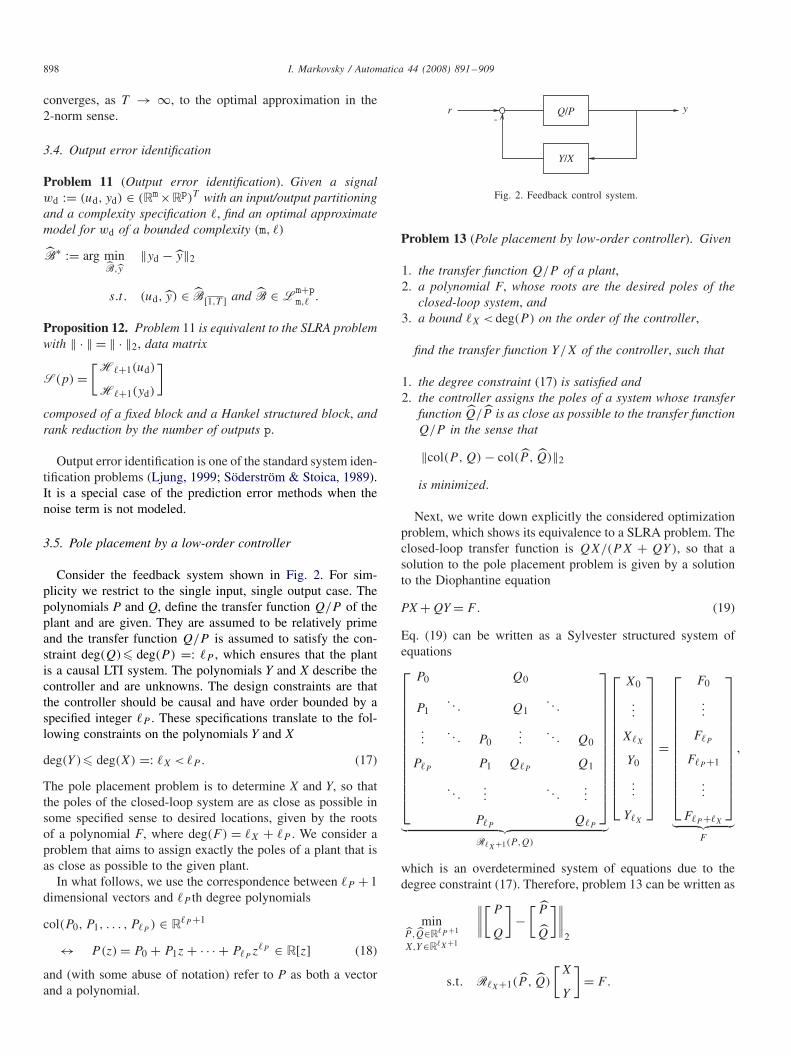
3.5. Pole placement by a low-order controller

Consider the feedback system shown in Fig. 2. For sim-plicity we restrict to the single input, single output case. Thepolynomials P and Q, define the transfer function Q/P of theplant and are given. They are assumed to be relatively primeand the transfer function Q/P is assumed to satisfy the con-straint deg(Q)� deg(P ) =: �P , which ensures that the plantis a causal LTI system. The polynomials Y and X describe thecontroller and are unknowns. The design constraints are thatthe controller should be causal and have order bounded by aspecified integer �P . These specifications translate to the fol-lowing constraints on the polynomials Y and X

deg(Y )� deg(X) =: �X < �P . (17)

The pole placement problem is to determine X and Y, so thatthe poles of the closed-loop system are as close as possible insome specified sense to desired locations, given by the rootsof a polynomial F, where deg(F ) = �X + �P . We consider aproblem that aims to assign exactly the poles of a plant that isas close as possible to the given plant.

In what follows, we use the correspondence between �P + 1dimensional vectors and �P th degree polynomials

col(P0, P1, . . . , P�P) ∈ R�P +1

↔ P(z) = P0 + P1z + · · · + P�Pz�P ∈ R[z] (18)

and (with some abuse of notation) refer to P as both a vectorand a polynomial.

-yr Q/P

Y/X

Fig. 2. Feedback control system.

Problem 13 (Pole placement by low-order controller). Given

1. the transfer function Q/P of a plant,2. a polynomial F, whose roots are the desired poles of the

closed-loop system, and3. a bound �X < deg(P ) on the order of the controller,

find the transfer function Y/X of the controller, such that

1. the degree constraint (17) is satisfied and2. the controller assigns the poles of a system whose transfer

function Q/P is as close as possible to the transfer functionQ/P in the sense that

‖col(P, Q) − col(P , Q)‖2

is minimized.

Next, we write down explicitly the considered optimizationproblem, which shows its equivalence to a SLRA problem. Theclosed-loop transfer function is QX/(PX + QY), so that asolution to the pole placement problem is given by a solutionto the Diophantine equation

PX + QY = F . (19)

Eq. (19) can be written as a Sylvester structured system ofequations⎡⎢⎢⎢⎢⎢⎢⎢⎢⎢⎢⎢⎢⎢⎣

P0 Q0

P1. . . Q1

. . .

.... . . P0

.... . . Q0

P�PP1 Q�P

Q1

. . ....

. . ....

P�PQ�P

⎤⎥⎥⎥⎥⎥⎥⎥⎥⎥⎥⎥⎥⎥⎦

︸︷︷︸R�X+1(P,Q)

⎡⎢⎢⎢⎢⎢⎢⎢⎢⎢⎢⎢⎢⎣

X0

...

X�X

Y0

...

Y�X

⎤⎥⎥⎥⎥⎥⎥⎥⎥⎥⎥⎥⎥⎦

=

⎡⎢⎢⎢⎢⎢⎢⎢⎢⎢⎢⎢⎢⎣

F0

...

F�P

F�P +1

...

F�P +�X

⎤⎥⎥⎥⎥⎥⎥⎥⎥⎥⎥⎥⎥⎦

︸︷︷︸F

,

which is an overdetermined system of equations due to thedegree constraint (17). Therefore, problem 13 can be written as

minP ,Q∈R�P +1

X,Y∈R�X+1

∥∥∥∥[

P

Q

]−

[P

Q

]∥∥∥∥2

s.t. R�X+1(P , Q)

[X

Y

]= F .



S(p) =[ [F0 F1 · · · F�P +�X

]R�

�X+1(P, Q)

]

composed of a fixed block and a Sylvester structured block, andrank reduction by 1.

3.6. Output only identification

The model class of autonomous LTI systems is Lp0,�. Ex-

cluding the cases of multiple poles, Lp0,� is equivalent to the

sum-of-damped exponentials model class, i.e., signals y that canbe represented in the form

y(t) =�∑

j=1

aj edj tei(�j t+�j ) (i : =√−1).

The parameters {aj , dj , �j , �j }�j=1 of the sum-of-damped ex-ponentials model have the following meaning: aj are ampli-tudes, dj damping, �j frequencies, and �j initial phases.

Problem 15 (Output only identification). Given a signal yd ∈(Rp)T and a complexity specification �, find an optimal ap-proximate model for yd of bounded complexity (0, �)

B∗ := arg minB,y

‖yd − y‖2

s.t. y ∈ B[1,T ] and B ∈ Lp0,�.

Proposition 16. Problem 15 is equivalent to the SLRA problemwith ‖ · ‖ = ‖ · ‖2, a Hankel structured data matrix S(p) =H�+1(yd), and rank reduction by the number of outputs p.

Output only identification is equivalent to approximate real-ization and finite time H2 model reduction. In the signal pro-cessing literature, the problem is known as linear prediction.

3.7. Finite impulse response system identification

Denote by FIRm,� the model class of finite impulse responseLTI systems with at most m inputs and lag at most �, i.e.,

FIRm,� := {B ∈ Lm,� |B has finite impulse response}.

Problem 17 (FIR identification). Given a signal wd :=(ud, yd) ∈ (Rm × Rp)T with an input/output partition and acomplexity specification �, find an optimal approximate FIRmodel for wd of bounded complexity (m, �)

B∗ := arg minB,w

‖wd − w‖2

s.t. w ∈ B[1,T ] and B ∈ FIRm,�.


S(p) =[ [yd(1) · · · yd(T − �)]

H�+1(ud)

],

composed of a fixed block and a Hankel structured block, andrank reduction by the number of outputs p.

For exact data, i.e., assuming that

yd(t) = (h � ud)(t) :=�∑

�=0

h(�)ud(t − �)

the FIR identification problem is equivalent to the deconvolu-tion problem: given the signals ud and yd := H � ud, find thesignal H. For noisy data, the FIR identification problem can beviewed as an approximate deconvolution problem. The approx-imation is in the sense of finding the nearest signals u and y tothe given ones ud and yd, such that y := H � u, for a signal H

with a given length �.

3.8. Harmonic retrieval

The aim of the harmonic retrieval problem is to approximatethe data by a sum of sinusoids. From a system theoretic pointof view, harmonic retrieval aims to approximate the data by amarginally stable autonomous model.

Problem 19 (Harmonic retrieval). Given a signal yd ∈ (Rp)T

and a complexity specification �, find an optimal approximatemodel for yd that is in the model class Lp

0,� and is marginallystable

B∗ := arg minB,y

‖yd − y‖2

s.t. y ∈ B[1,T ],

B ∈ Lp0,�, and B is marginally stable.

Due to the stability constraint, Problem (19) is not a specialcase of the SLRA problem. In the univariate case p = 1, how-ever, a necessary condition for an autonomous model B to bemarginally stable is that a kernel representation B(R) of B iseither palindromic,

R(z) :=�∑

i=0

ziRi is palindromic

: ⇐⇒ R�−i = Ri for i = 0, 1, . . . , �

or antipalindromic: R�−i = −Ri , for i = 0, 1, . . . , �. The an-tipalindromic case is nongeneric in the space of the marginallystable systems, so as relaxation of the stability constraint, wecan use the constraint that the kernel representation is palin-dromic.

Problem 20 (Harmonic retrieval, relaxed version, andscalar case). Given a signal yd ∈ (R)T and a complexity


specification �, find an optimal approximate model for ydthat is in the model class L1

0,� and has a palindromic kernelrepresentation

B∗ := arg minB,y

‖yd − y‖2

s.t. y ∈ B[1,T ],

B ∈ L10,� and B(R) = B are palindromic.

The constraint that R is palindromic can be expressed asa structural constraint on the data matrix, which reduces therelaxed harmonic retrieval problem to the SLRA problem.

Proposition 21. Problem 20 is equivalent to the SLRA problemwith ‖ · ‖=‖ ·‖2, structured data matrix composed of a Hankelnext to a Toeplitz block

S(p) = [H�+1(y) T�+1(y)],where

T�+1(y) :=

⎡⎢⎢⎢⎢⎢⎣

y�+1 y�+2 · · · yT

......

...

y2 y3 . . . yT −�+1

y1 y2 . . . yT −�

⎤⎥⎥⎥⎥⎥⎦ ,

and rank reduction by 1.

3.9. Approximate common divisor

Let GCD(a, b) be the greatest common divisor of the poly-nomials a and b and recall the one-to-one correspondence (18)between vectors in Rn+1 and nth degree polynomials.

Problem 22 (Approximate common divisor). Given vectorsa, b ∈ Rn+1 and an integer d ∈ N, find a vector

c∗ = arg mina,b∈Rn+1

c∈Rd+1

‖col(a, b) − col(a, b)‖2

s.t. c = GCD(a, b) and deg(c) = d .

Proposition 23. Problem 22 is equivalent to the SLRA problemwith ‖ · ‖ = ‖ · ‖2, Sylvester structure S(p) = R�

n−d+1(a, b),and rank reduction by 1.

For p×m matrix polynomials, the structure is block-Sylvesterand the necessary rank reduction is by p. For two variablepolynomial, the structure is block-Sylvester–Sylvester-block.

4. Algorithms

A few special SLRA problems have analytic solutions, seeSection 4.1, however in general the SLRA problem is NP-hard.There are three fundamentally different approaches for solvingit: convex relaxations, see Section 4.2, local optimization, see

Section 4.3, and global optimization. The approach that is cur-rently most developed (and that we describe in most details) isthe one using local optimization methods. Section 4.4 shows asimulation example of data fitting using the SLRA paradigm.

4.1. Special cases with known analytic solutions

The Eckart–Young–Mirsky theorem gives a solution to theunstructured low-rank approximation problem with Frobeniusnorm criterion in terms of the SVD.

Theorem 24 (Eckart–Young–Mirsky theorem). Let D=U�V �be the SVD of D ∈ Rd×N and partition the matrices U, �, andV as follows:

U =:

m p

[U1 U2, ],

�=:

m p[�1 0

0 �2

]m

p

,V=:

m p

[V1 V2 ],

where m ∈ N, 0�m� min(d, N), and p := d − m. Then therank-m matrix

D∗ = U1�1V�1

is such that

‖D − D∗‖F = minrank(D)�m

‖D − D‖F =√

�2m+1 + · · · + �2

d,

where diag(�1, . . . , �d) := �. The solution D∗ is unique if andonly if �m+1 �= �m.

As shown in Vanluyten, Willems, and De Moor (2005), thesolution D∗ is optimal with respect to any norm ‖ · ‖ that isinvariant under orthogonal transformations, i.e., satisfying therelation ‖UDV ‖ = ‖D‖, for any D and for any orthogonalmatrices U and V. Moreover, Theorem 24 can be generalizedto weighted norms of the form ‖Wl(D − D)Wr‖, where Wland Wr are positive definite weight matrices, see Section 5.1.These are the most general unstructured WLRA problems thatare known to have analytic solution in terms of the SVD.

Closely related to the basic low-rank approximation problemis the TLS problem: given matrices A ∈ RN×m and B ∈ RN×p,solve the optimization problem

minA,B,X

‖[A B] − [A B]‖F

s.t. AX = B.

The TLS problem is put forward in Golub and Van Loan (1980)for the case when B is a vector (system of equations with oneright-hand-side). The general case is treated in the monograph(Van Huffel & Vandewalle, 1991).

Theorem 25 (Solution to the TLS problem). Let

[A B] = U diag(�1, . . . , �m+p)V�


be the SVD of [A B] and partition the matrix V as follows

V:=

m p

[V1 V2, ] =:

m p[V11 V12

V21 V22

] m

p

.

A TLS solution exists if and only if the matrix V22 is nonsingular.In this case, a solution is

Xtls = −V12V−122 .

It is unique if and only if �m+1 �= �m.

As the solution to the basic low-rank approximation prob-lem, the solution to the TLS problem is also based on the SVDof the data matrix D� = [A B]. It involves, however, the ex-tra step of normalizing the matrix V2, so that its lower blockV22 becomes −I . This normalization imposes the input/outputstructure of the model, discussed in Section 1.2, and is the rea-son for the existence of nongeneric TLS problem. Note that theTLS approximation [A B] is the same as the low-rank approx-imation D∗�, provided the former exists. Therefore, if one isinterested in the best approximation of the data matrix [A B]and not in the solution X to the system AX ≈ B, there is noreason to do the normalization of V2.

We showed that some weighted unstructured low-rank ap-proximation problems have global analytic solution in terms ofthe SVD. Similar result exists for circulant SLRA. The resultis derived independently in the optimization community (Beck& Ben-Tal, 2006) and in the systems and control community(Vanluyten et al., 2005). If the approximation criterion is aunitarily invariant matrix norm, the unstructured low-rank ap-proximation (obtained for example from the truncated SVD) isunique. In the case of a circulant structure, it turns out that thisunique minimizer also has circulant structure, so the structureconstraint is satisfied without explicitly enforcing it.

An efficient computational way of obtaining the circulantstrcutured low-rank approximation is the fast Fourier transform.Consider the scalar case and let

Pk :=np∑

j=1

pj e−(2�i/np)kj

be the discrete Fourier transform of p. Denote with K thesubset of {1, . . . , np} consisting of the indices of the m largestelements of {|P1|, . . . , |Pnp |}. Assuming that K is uniquelydefined by the above condition, i.e., assuming that

k ∈ K and k′ /∈K �⇒ |Pk| > |Pk′ |,the solution p∗ of the SLRA problem with S a circulant matrixis unique and is given by

p∗ = 1

np

∑k∈K

Pke(2�i/np) kj .

4.2. Suboptimal solution methods

The SVD is at the core of many algorithms for approximatemodeling, most notably the methods based on balanced model

reduction, the subspace identification methods, and the MUSICand ESPRIT methods in signal processing. The reason for thisis that the SVD is a robust and efficient way of computing un-structured low-rank approximation of a matrix. In system iden-tification, signal processing, and computer algebra, however,the low-rank approximation is restricted to the class of matri-ces with specific (Hankel, Toeplitz, and Sylvester) structure.Ignoring the structure constraint renders the SVD-based meth-ods suboptimal with respect to a desired optimality criterion.

Except for the few special cases described in Section 4.1there are no global solution methods for general SLRA. TheSVD-based methods can be seen as relaxations of the originalNP-hard SLRA problem, obtained by removing the structureconstraint. Another approach is taken in Fazel (2002), whereconvex relaxations of the related (see Section 5.3) RMP are pro-posed. Convex relaxation methods give polynomial time sub-optimal solutions.

Presently there is no uniformly best method for comput-ing suboptimal SLRA. In the context of system identification(i.e., block-Hankel SLRA) several subspace and local opti-mization based methods are compared on practical data sets,see Markovsky, Willems, and De Moor (2006). In general, theheuristic methods are faster but less accurate than the methodsbased on local optimization, such as the prediction error meth-ods (Ljung, 1999) and the method of Markovsky, Van Huffel,and Pintelon (2005). It is a common practice to use a subop-timal solution obtained by a heuristic method as an initial ap-proximation for an optimization based method. Therefore, thetwo approaches complement each other.

4.3. Algorithms based on local optimization

Representing the constraint in a kernel form, the SLRA prob-lem becomes the following parameter optimization problem

minR, RR�=Im−r

(min

p‖p − p‖ s.t. RS(p) = 0

), (20)

which is a double minimization problem with a bilinear equalityconstraint. The outer minimization is over the model parameterR and the inner minimization is over the parameter estimatep. Since the mapping S is affine, there is an affine mappingG : R(m−r)×m → Rn(m−r)×np , such that

vec(RS(p)) = G(R)p for all p ∈ Rnp . (21)

A way to approach the double minimization is by solving theinner minimization analytically, which leads to a nonlinear leastsquares problem

minR, RR�=Im−r

vec� (RS (p)

) (G(R)G�(R)

)−1vec

(RS (p)

)(22)

for R only (Markovsky, Van Huffel, et al., 2005). The innerminimization problem is a least norm problem and can be giventhe interpretation of projecting the columns of S(p) onto thesubspace B := ker(R), for a given R ∈ Rm×(m−r). The pro-jection depends on the parameter R, which is the variable in


the outer optimization problem. For this reason, the method iscalled variable projections (Golub & Pereyra, 2003).

In order to evaluate the cost function for the outer minimiza-tion problem, we need to solve the inner minimization prob-lem, i.e., the least norm problem G(R)z = vec(RS(p)). Di-rect solution has computational complexity O(n3

p). The matrixG(R), however, is structured, which can be used in efficientcomputational method. The following result from Markovsky,Van Huffel, et al., (2005), shows that for a class of structuresS, the structure of the matrix GG� that appears in the solutionof the least norm problem is block-Toeplitz and block-banded.

Theorem 26. Assume that S is composed of blocks that areblock-Hankel, unstructured, or fixed, i.e.,

S(p) = [S1(p) · · ·Sq(p)], (23)

where S1(p) is block-Hankel, unstructured, or does not dependon p. Then the matrix GG�, where G is defined in (21) is block-Toeplitz and block-banded structured.

The implication of Theorem 26 is that for the class of struc-tures (23), efficient O(np) cost function evaluation can bedone by Cholesky factorization of a block-Toeplitz banded ma-trix. The SLICOT library includes high quality FORTRAN im-plementation of algorithms for this problem. It is used in asoftware package for solving SLRA problems, based on theLevenberg–Marquardt algorithm, implemented in MINPACK(Markovsky, Van Huffel, et al., 2005; Markovsky & Van Huffel,2005). This algorithm is globally convergent with a superlinearconvergence rate.

Some SLRA problems can be solved by an algorithm basedon the alternating least squares method. Consider the approxi-mate deconvolution problems

minu,y,h

‖col(ud, yd) − col(u, y)‖2

s.t. h�T�+1(u) = y�. (24)

It is equivalent to the problem

minu,h

∥∥∥∥[ud

yd

]−

[u

T��+1(u)h

]∥∥∥∥2

. (25)

The alternating projections algorithm, see Algorithm 1, is basedon the fact that problem (25) is a standard least squares problemfor given u and for given h. Minimizing alternatively over hwith u fixed to its value from the previous iteration step, andover u with h fixed its value from the previous iteration step, weobtain a sequence of approximations (u(k), h(k)), k = 1, 2, . . .

that corresponds to a nonincreasing sequence of cost functionvalues. The alternating projections algorithm is also globallyconvergent, however, its local convergence rate is only linear.

In this section we described the variable projections andalternating projections methods for solving the SLRA prob-lem. Using global optimization methods, e.g., the branch andbound type algorithms, instead of local optimization methodsis also an option. Efficient cost function evaluation, obtained byexploiting the matrix structure, is of prime importance in the

application of global optimization methods as well. The num-ber of cost function evaluations required for finding a globalsolution, however, is likely to be much higher than the one re-quired for finding a locally optimal solution.

Algorithm 1. Alternating projections algorithm for solving theapproximate deconvolution problem (24).Input: Data ud, yd and convergence tolerance ε.1: Set k := 0 and compute an initial approxima-

tion h(0), u(0), y(0), e.g., by solving the TLS problemT�(ud)h = yd.

2: repeat3: k := k + 1.4: Solve the least squares problem in u

u(k) := arg minu

∥∥∥∥[ud

yd

]−

[I

T (h(k−1))

]u

∥∥∥∥2

,

where T (h) is a matrix depending on h, such thatT�

�+1(u)h = T (h)u.5: Solve the least squares problem in h

h(k) := arg minh

‖yd − T��+1(u

(k))h‖2.

6: y(k) := T��+1(u

(k))h(k).7: until ‖col(u(k−1), y(k−1)) − col(u(k), y(k))‖ < ε

Output: A locally optimal solution h∗ := h(k), u∗ := u(k),and y∗ := y(k) of (24).

4.4. Simulation example

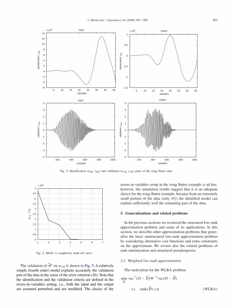
The database for identification of systems (DAISY)(De Moor, 2005) contains real-life and simulated benchmarkdata sets. In this section, we use the DAISY data set called“Wing flutter data”, which consist of T = 1024 samples of theinput and the output of the system to be identified.2 We dividethe data wd = (ud, yd) into identification widt = (uidt, yidt) andvalidation wval =(uval, yval) parts, see Fig. 3. An optimal modelB∗ in the sense of Problem 5 is identified from widt usingProposition 6 and the software package of (Markovsky & VanHuffel, 2005) and is validated on wval, using the fitting error

e(wval, B∗) := min

w∗∈B∗‖wval − w∗‖. (26)

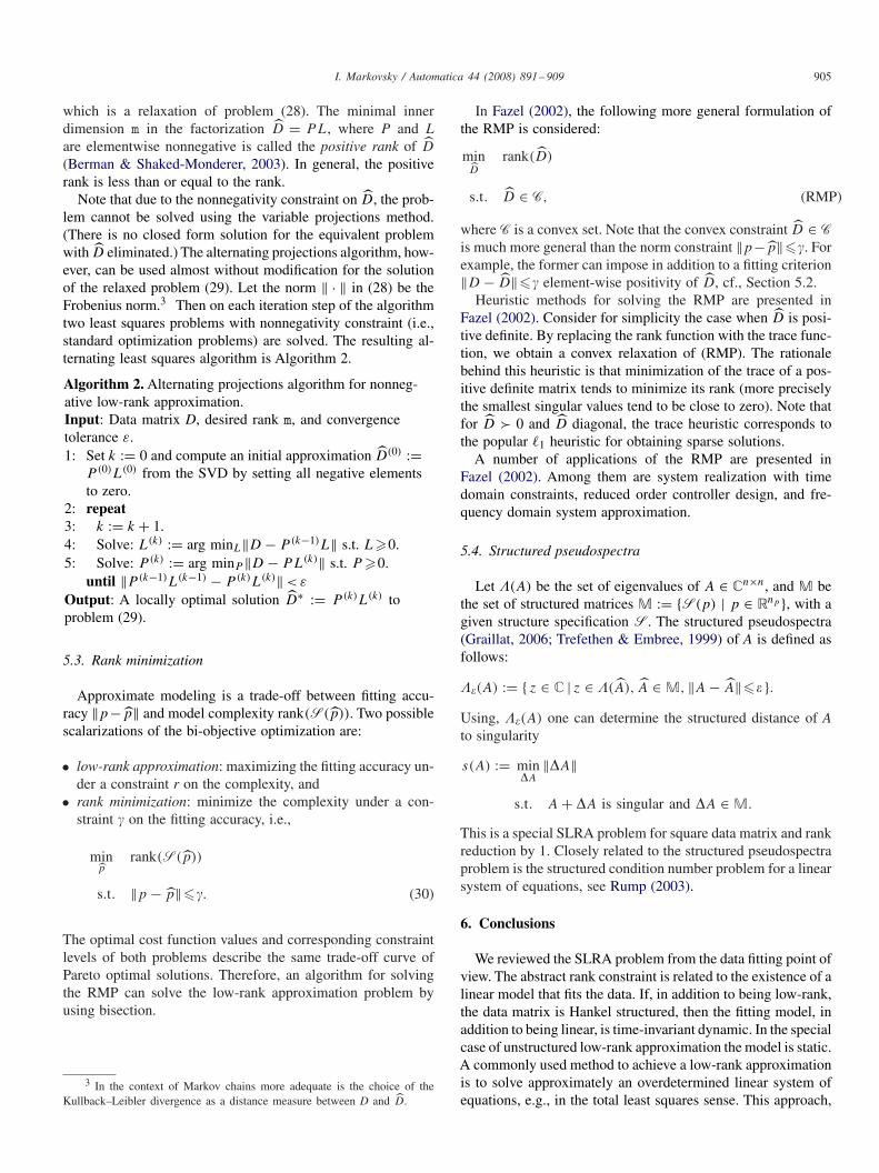
The optimal model is searched in the LTI model class Lm,�,where m = 1 is fixed by the given data but � is an unknownparameter. We choose � from the fitting error e(widt, B

∗) vscomplexity � trade-off curve, see Fig. 4. The “best” value for theparameter � is selected visually and corresponds to the cornerof the “L” shaped trade-off curve. In the particular example,we choose � = 4, so the considered model class is L1,4. Theoptimal model B∗ in L1,4 is B∗ = ker(R∗(�)), where

R∗(z) = [9.55 − 0.09]z0 + [−32.18 1.50]z1

+ [43.77 − 3.56]z2 + [−28.62 3.05]z3

+ [7.57 − 1]z4.

2 The description of this data set in DAISY says “Due to industrialsecrecy agreements we are not allowed to reveal more details.”


5 10 15 20 25 30 35 40-6

-4

-2

0

2

4

6

8

10

12

14

x 104

samples

input

identification,

uid

t

5 10 15 20 25 30 35 40

-1.5

-1

-0.5

0

0.5

1

x 103

samples

identication,

yid

t

output

200 400 600 800 1000-4

-3

-2

-1

0

1

2

3

4

input

valid

ation,

uva

l

200 400 600 800 1000-4

-3

-2

-1

0

1

2

3

4

samples

output

valid

ation,

yva

l

samples

Fig. 3. Identification (uidt, yidt) and validation (uval, yval) parts of the wing flutter data.

1 2 3 4 5 6 70

0.5

1

1.5

2

2.5

3

3.5

4.

4.5

5

x 104

l

||wid

t - w

* ||^

Fig. 4. Misfit vs complexity trade-off curve.

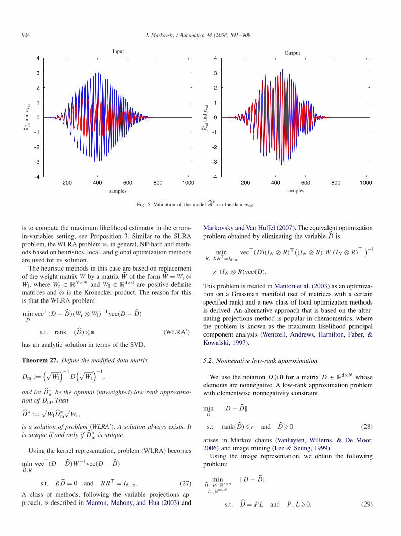
The validation of B∗ on wval is shown in Fig. 5. A relativelysimple (fourth order) model explains accurately the validationpart of the data in the sense of the error criterion (26). Note thatthe identification and the validation criteria are defined in theerrors-in-variables setting, i.e., both the input and the outputare assumed perturbed and are modified. The choice of the

errors-in-variables setup in the wing flutter example is ad hoc,however, the simulation results suggest that it is an adequatechoice for the wing flutter example, because from an extremelysmall portion of the data (only 4%) the identified model canexplain sufficiently well the remaining part of the data.

5. Generalizations and related problems

In the previous sections we reviewed the structured low-rankapproximation problem and some of its applications. In thissection, we describe other approximation problems that gener-alize the basic unstructured low-rank approximation problemby considering alternative cost functions and extra constraintson the approximant. We review also the related problems ofrank minimization and structured pseudospectra.

5.1. Weighted low-rank approximation

The motivation for the WLRA problem

minD

vec�(D − D)W−1vec(D − D)

s.t. rank(D)�m (WLRA)


200 400 600 800 1000-4

-3

-2

-1

0

1

2

3

4Input

u val

and

uva

l

200 400 600 800 1000-4

-3

-2

-1

0

1

2

3

4

samples

Output

y val

and

yva

l

samples

**^ ^

Fig. 5. Validation of the model B∗

on the data wval.

is to compute the maximum likelihood estimator in the errors-in-variables setting, see Proposition 3. Similar to the SLRAproblem, the WLRA problem is, in general, NP-hard and meth-ods based on heuristics, local, and global optimization methodsare used for its solution.

The heuristic methods in this case are based on replacementof the weight matrix W by a matrix W of the form W = Wr ⊗Wl, where Wr ∈ RN×N and Wl ∈ Rd×d are positive definitematrices and ⊗ is the Kronecker product. The reason for thisis that the WLRA problem

minD

vec�(D − D)(Wr ⊗ Wl)−1vec(D − D)

s.t. rank (D)�m (WLRA′)

has an analytic solution in terms of the SVD.

Theorem 27. Define the modified data matrix

Dm :=(√

Wl

)−1D

(√Wr

)−1,

and let D∗m be the optimal (unweighted) low rank approxima-

tion of Dm. Then

D∗ := √WlD

∗m

√Wr,

is a solution of problem (WLRA′). A solution always exists. Itis unique if and only if D∗

m is unique.

Using the kernel representation, problem (WLRA) becomes

minD,R

vec�(D − D)W−1vec(D − D)

s.t. RD = 0 and RR� = Id−m. (27)

A class of methods, following the variable projections ap-proach, is described in Manton, Mahony, and Hua (2003) and

Markovsky and Van Huffel (2007). The equivalent optimizationproblem obtained by eliminating the variable D is

minR, RR�=Id−m

vec�(D)(IN ⊗ R)�((IN ⊗ R) W (IN ⊗ R)

� )−1

× (IN ⊗ R)vec(D).

This problem is treated in Manton et al. (2003) as an optimiza-tion on a Grassman manifold (set of matrices with a certainspecified rank) and a new class of local optimization methodsis derived. An alternative approach that is based on the alter-nating projections method is popular in chemometrics, wherethe problem is known as the maximum likelihood principalcomponent analysis (Wentzell, Andrews, Hamilton, Faber, &Kowalski, 1997).

5.2. Nonnegative low-rank approximation

We use the notation D�0 for a matrix D ∈ Rd×N whoseelements are nonnegative. A low-rank approximation problemwith elementwise nonnegativity constraint

minD

‖D − D‖

s.t. rank(D)�r and D�0 (28)

arises in Markov chains (Vanluyten, Willems, & De Moor,2006) and image mining (Lee & Seung, 1999).

Using the image representation, we obtain the followingproblem:

minD, P∈Rd×m

L∈Rm×N

‖D − D‖

s.t. D = PL and P, L�0, (29)


which is a relaxation of problem (28). The minimal innerdimension m in the factorization D = PL, where P and Lare elementwise nonnegative is called the positive rank of D

(Berman & Shaked-Monderer, 2003). In general, the positiverank is less than or equal to the rank.

Note that due to the nonnegativity constraint on D, the prob-lem cannot be solved using the variable projections method.(There is no closed form solution for the equivalent problemwith D eliminated.) The alternating projections algorithm, how-ever, can be used almost without modification for the solutionof the relaxed problem (29). Let the norm ‖ · ‖ in (28) be theFrobenius norm.3 Then on each iteration step of the algorithmtwo least squares problems with nonnegativity constraint (i.e.,standard optimization problems) are solved. The resulting al-ternating least squares algorithm is Algorithm 2.

Algorithm 2. Alternating projections algorithm for nonneg-ative low-rank approximation.Input: Data matrix D, desired rank m, and convergencetolerance ε.1: Set k := 0 and compute an initial approximation D(0) :=

P (0)L(0) from the SVD by setting all negative elementsto zero.

2: repeat3: k := k + 1.4: Solve: L(k) := arg minL‖D − P (k−1)L‖ s.t. L�0.5: Solve: P (k) := arg minP ‖D − PL(k)‖ s.t. P �0.

until ‖P (k−1)L(k−1) − P (k)L(k)‖ < ε

Output: A locally optimal solution D∗ := P (k)L(k) toproblem (29).

5.3. Rank minimization

Approximate modeling is a trade-off between fitting accu-racy ‖p− p‖ and model complexity rank(S(p)). Two possiblescalarizations of the bi-objective optimization are:

• low-rank approximation: maximizing the fitting accuracy un-der a constraint r on the complexity, and

• rank minimization: minimize the complexity under a con-straint � on the fitting accuracy, i.e.,

minp

rank(S(p))

s.t. ‖p − p‖��. (30)

The optimal cost function values and corresponding constraintlevels of both problems describe the same trade-off curve ofPareto optimal solutions. Therefore, an algorithm for solvingthe RMP can solve the low-rank approximation problem byusing bisection.

3 In the context of Markov chains more adequate is the choice of theKullback–Leibler divergence as a distance measure between D and D.

In Fazel (2002), the following more general formulation ofthe RMP is considered:

minD

rank(D)

s.t. D ∈ C, (RMP)

where C is a convex set. Note that the convex constraint D ∈ Cis much more general than the norm constraint ‖p−p‖��. Forexample, the former can impose in addition to a fitting criterion‖D − D‖�� element-wise positivity of D, cf., Section 5.2.

Heuristic methods for solving the RMP are presented inFazel (2002). Consider for simplicity the case when D is posi-tive definite. By replacing the rank function with the trace func-tion, we obtain a convex relaxation of (RMP). The rationalebehind this heuristic is that minimization of the trace of a pos-itive definite matrix tends to minimize its rank (more preciselythe smallest singular values tend to be close to zero). Note thatfor D � 0 and D diagonal, the trace heuristic corresponds tothe popular �1 heuristic for obtaining sparse solutions.

A number of applications of the RMP are presented inFazel (2002). Among them are system realization with timedomain constraints, reduced order controller design, and fre-quency domain system approximation.

5.4. Structured pseudospectra

Let (A) be the set of eigenvalues of A ∈ Cn×n, and M bethe set of structured matrices M := {S(p) | p ∈ Rnp }, with agiven structure specification S. The structured pseudospectra(Graillat, 2006; Trefethen & Embree, 1999) of A is defined asfollows:

(A) := { z ∈ C | z ∈ (A), A ∈ M, ‖A − A‖� }.Using, (A) one can determine the structured distance of Ato singularity

s(A) := min�A

‖�A‖

s.t. A + �A is singular and �A ∈ M.

This is a special SLRA problem for square data matrix and rankreduction by 1. Closely related to the structured pseudospectraproblem is the structured condition number problem for a linearsystem of equations, see Rump (2003).

6. Conclusions

We reviewed the SLRA problem from the data fitting point ofview. The abstract rank constraint is related to the existence of alinear model that fits the data. If, in addition to being low-rank,the data matrix is Hankel structured, then the fitting model, inaddition to being linear, is time-invariant dynamic. In the specialcase of unstructured low-rank approximation the model is static.A commonly used method to achieve a low-rank approximationis to solve approximately an overdetermined linear system ofequations, e.g., in the total least squares sense. This approach,


however, imposes an additional input/output structure on themodel that might not be relevant in the application at hand.

There are numerous applications of SLRA in system the-ory, signal processing, and computer algebra. The data matrixis block structured where each of the blocks is either block-Hankel, unstructured, or fixed. The model being multivariableimplies that the data matrix is block-Hankel structured with un-structured block elements. The model being multidimensionalimplies that the data matrix is block-Hankel structured withHankel structured block elements. We reviewed algorithms forsolving low-rank approximation problems, based on the vari-able projections and alternating projections methods.

Finally, we showed generalizations and related problems.The generalizations consider different approximation criteriaand constraints on the data matrix. Closely related to struc-tured low-rank minimization are the rank minimization and thestructured pseudo-spectra problems.

Appendix A. Kernel, image, and input/output representa-tions

A.1. Linear static models

A static model B with d variables is a subset of Rd. A linearstatic model with d variables is a subspace of Rd. Three basicrepresentations of a linear static model B ⊆ Rd are the kernel,image, and input/output ones:

• kernel representation B = ker(R), with R ∈ Rp×d,• image representation B = image(P ), with P ∈ Rd×m, and• input/output representation

Bi/o(X, �) := {d := �col(di, do) ∈ Rd |di ∈ Rm, do = X�di}

with parameters X ∈ Rm×p and a permutation matrix �.If the parameter � in an input/output representation is not

specified, then by default it is � = I , i.e., the first m variablesare assumed inputs and the other p := d−m outputs. In terms ofthe data matrix D, the input/output representation is the systemof equations AX ≈ B, where [A B]�� := D�. Thus solvingAX ≈ B approximately by least squares, TLS, or any othermethod is equivalent to solving a low-rank approximation usingan input/output representation.

If the parameters R, P, and X describe the same system B,then they are related. Let � = I and define the partitioning

R := [Ri Ro] where Ro ∈ Rp×p

and

P :=[Pi

Po

]where Pi ∈ Rm×m.

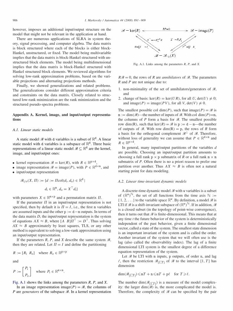
Fig. A.1 shows the links among the parameters R, P, and X.In an image representation image(P ) = B, the columns of

P are generators of the subspace B. In a kernel representation

Fig. A.1. Links among the parameters R, P, and X.

RB = 0, the rows of R are annihilators of B. The parametersR and P are not unique due to:

1. non-minimality of the set of annihilators/generators of B,and

2. change of basis: ker(R) = ker(UR), for all U, det(U) �= 0;and image(P ) = image(PV ), for all V, det(V ) �= 0.

The smallest possible col dim(P ), such that image(P ) = B ism := dim(B)—the number of inputs ofB. With col dim(P )=m,the columns of P form a basis for B. The smallest possiblerow dim(R), such that ker(R) =B is p := d− m—the numberof outputs of B. With row dim(R) = p, the rows of R forma basis for the orthogonal complement B⊥ of B. Therefore,without loss of generality we can assume that P ∈ Rd×m andR ∈ Rp×d.

In general, many input/output partitions of the variables dare possible. Choosing an input/output partition amounts tochoosing a full rank p × p submatrix of R or a full rank m × msubmatrix of P. Often there is no a priori reason to prefer onepartition over another. Thus AX ≈ B is often not a naturalstarting point for data modeling.

A.2. Linear time-invariant dynamic models

A discrete-time dynamic model B with w variables is a subsetof (Rw)N, the set of all functions from the time axis N :={ 1, 2, . . . } to the variable space Rw. By definition, a model B isLTI if B is a shift-invariant subspace of (Rw)N. If in addition, Bis a closed subset (in the topology of point-wise convergence),then it turns out that B is finite-dimensional. This means that atany time t the future behavior of the system is deterministicallyindependent of the past behavior, given a finite dimensionalvector, called a state of the system. The smallest state dimensionis an important invariant of the system and is called the order.Another invariant of the system that we will often use is thelag (also called the observability index). The lag of a finitedimensional LTI system is the smallest degree of a differenceequation representation of the system.

Let B be LTI with m inputs, p outputs, of order n, and lagl, then the restriction B[1,T ] of B to the interval [1, T ] hasdimension

dim(B[1,T ])�mT + n�mT + p� for T ��.

The number dim(B[1,T ]) is a measure of the model complex-ity: the larger dim(B) is, the more complicated the model is.Therefore, the complexity of B can be specified by the pair


(m, n) or alternatively by the pair (m, �). We use the notationLw

m,� for the LTI model class with bounded complexity: m orless inputs and lag at most �.

Three common representations for LTI model are:

• kernel representation

R0w(t) + R1w(t + 1) + · · · + R�w(t + �) = 0,

with parameter the polynomial matrix R(z) := ∑�i=0 Riz

i ,• impulse response representation

w = �col(u, y), y(t) =∞∑

�=0

H(�)u(t − �),

with parameters the signal H : N → Rp×m and permutationmatrix �, and

• input/state/output representation

w = �col(u, y),x(t + 1) = Ax(t) + Bu(t)

y(t) = Cx(t) + Du(t),

with parameters (A, B, C, D) and permutation matrix �.

Transitions among the parameters R, H, and (A, B, C, D)

are classical problems, e.g., going from R or H to (A, B, C, D)

are realization problems.

Appendix B. Proofs

B.1. Proof of Proposition 3

The probability density function of the observation vectorvec(D) is

pB,D(vec(D))

=

⎧⎪⎪⎪⎨⎪⎪⎪⎩

const · exp − 1

2v‖vec(D) − vec(D)‖2

W,

if image(D) ⊂ B and dim(B)�m

0, otherwise,

where “const” is a term that does not depend on D and B. Thelog-likelihood function is

�(B, D) =

⎧⎪⎪⎪⎨⎪⎪⎪⎩

const − 1


W

if image(D) ⊂ B and dim(B)�m

−∞ otherwise,

and the maximum likelihood estimation problem is

minB,D

1


W

s.t. image(D) ⊂ B and dim(B)�m,

which is an equivalent problem to Problem 2 with ‖·‖=‖·‖W .

Remark 28. An image representation image(P ∗) of the opti-mal approximate model B∗ can be obtained from the solutionD∗ to the low-rank approximation problem by doing a rankrevealing factorization D∗ = P ∗L∗, and a kernel representa-tion ker(R∗) can be obtained by computing a basis for the leftnullspace of D∗. The parameters P and R, however, can beused as optimization variables in the low-rank approximationproblem, in which case they are obtained as a by-product fromthe algorithm solving the low-rank approximation problem.


It is analogous to the proof of Proposition 3 and is skipped.

Remark 29. Computing the optimal approximate model B∗from the solution p∗ to the SLRA problem is an exact iden-tification problem, see Markovsky, Willems, Van Huffel et al.(2006, Chapter 8), Van Overschee and De Moor (1996, Chapter2), and Markovsky, Willems, Rapisarda, and De Moor (2005).As in the static approximation problem, however, the parame-ter of a model representation is an optimization variable of theoptimization problem, used for solving the SLRA problem, sothat a representation of the model is obtain directly from theoptimization solver.


The proposition follows from the equivalence

H is the impulse response of B ∈ Lm,�

⇐⇒ rank(H�+1(�H ))�m�,

which is a well-known fact from realization theory, see, e.g.,Markovsky, Willems, Van Huffel et al. (2006, Section 8.7).Obtaining the model B from the solution to the SLRA problemis the LTI system realization problem.


The problem is equivalent to the approximate real-ization problem with Hd being the impulse response ofBd, see Markovsky, Willems, Van Huffel et al. (2006,Section 11.4).


The proposition is based on the equivalence

(ud, y) ∈ B[1,T ] and B ∈ Lm,�

⇐⇒ rank

([H�+1(ud)

H�+1(y)

])�m(� + 1) + p�,

which is a corollary of the following lemma.

Lemma 30. The signal w ∈ B[1,T ] and B ∈ Lwm,� if and only

if rank(H�+1(w))�m(� + 1) + (w − m)�.


Proof. (⇒) Assume that w ∈ B[1,T ], B ∈ Lm,� and let B(R),

with R(z) = ∑�i=0z

iRi ∈ Rg×w[z] full row rank, be a kernelrepresentation of B. The assumption B ∈ Lm,� implies thatg�p := w − m. From w ∈ B[1,T ], we have that

[R0 R1 · · · R�]H�+1(w) = 0,

which implies that rank(H�+1(w))�m(� + 1) + p�.(⇐) Assume that rank(H�+1(w))�m(�+1)+p�. Then there

is a full row rank matrix R := [R0 R1 · · · R�] ∈ Rp×w(�+1),such that RH�+1(w)=0. Define the polynomial matrix R(z)=∑�

i=0ziRi . Then the system B induced by R(z) via the kernel

representation (13) is such that w ∈ B and B ∈ Lm,�. �


The problem is equivalent to the approximate realizationproblem, see Markovsky, Willems, Van Huffel et al. (2006, Sec-tion 11.4).



w ∈ B[1,T ] and B ∈ FIRm,�

⇐⇒ rank

([ [y(1) · · · y(T − �)]H�+1(u)

])�m(� + 1).

In order to show it, let

H = (H(0), H(1), . . . , H(�), 0, 0, . . .)

be the impulse response of B ∈ FIRm,�. The signal w = (u, y)

is a trajectory of B if and only if

[H(�) · · · H(1) H(0)]H�+1(u) = [y(1) · · · y(T − �)]or equivalently

[−Ig H(�) · · · H(1) H(0)][ [y(1) · · · y(T − �)]

H�+1(u)

]= 0.

The assumption B ∈ FIRm,� implies that g�p. Therefore,

rank

([ [y(1) · · · y(T − �)]H�+1(u)

])�m(� + 1).



y ∈ B[1,T ], B ∈ L10,� and B(R) = B is palindromic

⇐⇒ rank([H�+1(y) T�+1(y)

])��.

In order to show it, let B(R), with R(z) = ∑�i=0z

iRi full rowrank, be a kernel representation of B ∈ L1

0,�. Then y ∈ B[1,T ]

is equivalent to [R0 R1 · · · R�]H�+1(y) = 0. If, in addition,R is palindromic, then

[R� · · · R1 R0]H�+1(y) = 0

⇐⇒ [R0 R1 · · · R�]T�+1(y) = 0.

We have that

[R0 R1 · · · R�][H�+1(y) T�+1(y)] = 0. (B.1)

which is equivalent to rank([H�+1(y) T�+1(y)])��. Con-versely, (B.1) implies y ∈ B[1,T ] and R palindromic.


The proposition follows from the Sylvester test for co-primness of two scalar polynomials

c = GCD(a, b) and deg(c)�d

⇐⇒ rank(Rn−d+1(a, b))�n − d.

References

Beck, A., & Ben-Tal, A. (2006). A global solution for the structured total leastsquares problem with block circulant matrices. SIAM Journal of MatrixAnalysis and Applications, 27(1), 238–255.

Berman, A., & Shaked-Monderer, N. (2003). Completely positive matrices.Singapore: World Scientific.

Boyd, S., & Vandenberghe, L. (2004). Convex optimization. Cambridge:Cambridge University Press.

Chandrasekaran, S., Gu, M., & Sayed, A. (1998). A stable and efficientalgorithm for the indefinite linear least-squares problem. SIAM Journal ofMatrix Analysis and Applications, 20(2), 354–362.

De Moor, B. (1993). Structured total least squares and L2 approximationproblems. Linear Algebra and Its Applications, 188–189, 163–207.

De Moor, B. (1994). Total least squares for affinely structured matrices andthe noisy realization problem. IEEE Transactions on Signal Processing,42(11), 3104–3113.

De Moor B. (2005), Dalsy: Database for the identification of systems,Department of Electrical Engineering, K.U. Leuven〈www.esat.kuleuven.ac.be/sista.daisy/〉.

Degroat, R., & Dowling, E. (1991). The data least squares problem andchannel equalization. IEEE Transactions on Signal Processing, 41, 407–411.

Eckart, G., & Young, G. (1936). The approximation of one matrix by anotherof lower rank. Psychometrika, 1, 211–218.

Fazel, M. (2002). Matrix rank minimization with applications. Ph.D. thesis,Electrical Engineering Department, Stanford University.

Golub, G., & Pereyra, V. (2003). Separable nonlinear least squares: Thevariable projection method and its applications. Institute of Physics, InverseProblems, 19, 1–26.

Golub, G., & Van Loan, C. (1980). An analysis of the total least squaresproblem. SIAM Journal on Numerical Analysis, 17, 883–893.

Graillat, S. (2006). A note on structured pseudospectra. Journal ofComputational and Applied Mathematics, 191, 68–76.

Ho, B. L., & Kalman, R. E. (1966). Effective construction of linear state-variable models from input/output functions. Regelungstechnik, 14(12),545–592.

Kukush, A., Markovsky, I., & Van Huffel, S. (2005). Consistency of thestructured total least squares estimator in a multivariate errors-in-variablesmodel. Journal of Statistical Planning and Inference, 133(2), 315–358.

Kung, S. (1978). A new identification method and model reduction algorithmvia singular value decomposition. In Proceedings of the 12th Asilomarconference on circuits, systems, and computers (pp. 705–714). PacificGrove, CA.


Lee, D., & Seung, H. (1999). Learning the parts of objects by non-negativematrix factorization. Nature, 401, 788–791.

Ljung, L. (1999). System identification: Theory for the user. Upper SaddleRiver, NJ: Prentice-Hall.

Manton, J., Mahony, R., & Hua, Y. (2003). The geometry of weightedlow-rank approximations. IEEE Transactions on Signal Processing, 51(2),500–514.

Markovsky, I., & Van Huffel, S. (2005). High-performance numericalalgorithms and software for structured total least squares. Journal ofComputational and Applied Mathematics, 180(2), 311–331.

Markovsky, I., & Van Huffel, S. (2007). Left vs right representations forsolving weighted low rank approximation problems. Linear Algebra andIts Applications, 422, 540–552.

Markovsky, I., Van Huffel, S., & Pintelon, R. (2005). Block-Toeplitz/Hankelstructured total least squares. SIAM Journal of Matrix Analysis andApplications, 26(4), 1083–1099.

Markovsky, I., Willems, J. C., De Moor, B. (2006). Comparison ofidentification algorithms on the database for system identification DAISY.In Proceedings of the 17th symposium on mathematical theory of networksand systems (pp. 2858–2869). Kyoto, Japan.

Markovsky, I., Willems, J. C., Rapisarda, P., & De Moor, B. (2005).Algorithms for deterministic balanced subspace identification. Automatica,41(5), 755–766.

Markovsky, I., Willems, J. C., Van Huffel, S., De Moor, B. (2006). Exactand approximate modeling of linear systems: A behavioral approach. InMonographs on mathematical modeling and computation, vol. 11. SIAM.

Markovsky, I., Willems, J. C., Van Huffel, S., De Moor, B., & Pintelon,R. (2005). Application of structured total least squares for systemidentification and model reduction. IEEE Transactions on AutomaticControl, 50(10), 1490–1500.

Pintelon, R., & Schoukens, J. (2001). System identification: A frequencydomain approach. Piscataway, NJ: IEEE Press.

Polderman, J., & Willems, J. C. (1998). Introduction to mathematical systemstheory. New York: Springer.

Roorda, B. (1995). Algorithms for global total least squares modelling offinite multivariable time series. Automatica, 31(3), 391–404.

Roorda, B., & Heij, C. (1995). Global total least squares modeling ofmultivariate time series. IEEE Transactions on Automatic Control, 40(1),50–63.

Rump, S. (2003). Structured perturbations part I: Normwise distances. SIAMJournal of Matrix Analysis and Applications, 25, 1–30.

Söderström, T. (2007). Errors-in-variables methods in system identification.Automatica, 43, 939–958.

Söderström, T., & Stoica, P. (1989). System identification. NJ: Prentice-Hall.Trefethen, L. N., & Embree, M. (1999). Spectra and pseudospectra: The

behavior of nonnormal matrices and operators. Princeton, NJ: PrincetonUniversity Press.

Van Huffel, S., & Van dewalle, J. (1991). The total least squares problem:Computational aspects and analysis. Philadelphia: SIAM.

Van Overschee, P., & De Moor, B. (1996). Subspace identification for linearsystems: theory, implementation, applications. Boston: Kluwer.

Vanluyten, B., Willems, J. C., De Moor, B. (2005). Model reduction ofsystems with symmetries. In Proceedings of the 44th IEEE conference ondecision and control (pp. 826–831). Seville, Spain.

Vanluyten, B., Willems, J. C., & De Moor, B. (2006). Matrix factorization andstochastic state representations. In Proceedings of the 45th IEEE conferenceon decision and control (pp. 4188–4193). San Diego, California.

Wentzell, P., Andrews, D., Hamilton, D., Faber, K., & Kowalski, B.(1997). Maximum likelihood principle component analysis. Journal ofChemometrics, 11, 339–366.

Willems, J. C. (1986, 1987). From time series to linear system—Part I. Finitedimensional linear time invariant systems, Part II. Exact modelling, Part III.Approximate modelling. Automatica, 22, 23, 561–580, 675–694, 87–115.

Willems, J. C. (1991). Paradigms and puzzles in the theory of dynamicalsystems. IEEE Transactions on Automatic Control, 36(3), 259–294.

Ivan Markovsky obtained MS degree in Con-trol and Systems Engineering in 1998 fromthe Technical University of Sofia, Bulgaria andPh.D. degree in 2005 from the Katholieke Uni-versiteit Leuven, Belgium. Since January 2007he is a lecturer at the School of Electronics andComputer Science, University of Southampton,UK. His research work is focused on identi-fication methods in the behavioral setting anderrors-in-variables estimation problems. He isa coauthor of the book “Exact and Approxi-mate Modeling of Linear Systems: A BehavioralApproach” (SIAM, Philadelphia, 2006).

Documents

Structured low-rank approximation and its applications