STUDIES ON SOME ASPECTS OF COMPOSITE MACHINING

Thesis Submitted in Partial Fulfillment of the Requirements for the Degree of

Master of Technology (M. Tech.) by Research In

Production Engineering By

Ms. ANKITA SINGH

Roll No. 610ME306

Under the Guidance of

DR. SAURAV DATTA

NATIONAL INSTITUTE OF TECHNOLOGY

ROURKELA 769008, INDIA

ii

NATIONAL INSTITUTE OF TECHNOLOGY

ROURKELA 769008, INDIA

Certificate of Approval

This is to certify that the thesis entitled STUDIES ON SOME ASPECTS OF

COMPOSITE MACHINING submitted by Ankita Singh has been carried out under

my supervision in partial fulfillment of the requirements for the Degree of Master of

Technology (By Research) in Production Engineering at National Institute of

Technology, Rourkela, and this work has not been submitted elsewhere before for

any other academic degree/diploma.

------------------------------------------

Dr. Saurav Datta

Assistant Professor Department of Mechanical Engineering

National Institute of Technology, Rourkela-769008

iii

Acknowledgement

In pursuit of this academic endeavor I feel that I have been especially fortunate as

inspiration, guidance, direction, co-operation, love and care all came in my way in

abundance and it seems almost an impossible task for me to acknowledge the same in

adequate terms.

It gives me immense pleasure to express my deep sense of gratitude to my

supervisor Prof. Saurav Datta, Assistant Professor, Department of Mechanical

Engineering, NIT Rourkela, for his invaluable guidance, motivation, constant inspiration

and above all for his ever co-operating attitude that enabled me in bringing up this

thesis in the present form. Above all, he provided me unflinching encouragement and

support in various ways which exceptionally inspire and enrich my growth as a

student, a researcher.

I specially acknowledge Prof. S. S. Mahapatra, Professor, Department of Mechanical

Engineering, NIT Rourkela, for his advice, supervision, and crucial contribution, as

and when required during this research. I am proud to express that I had

opportunity to work with an exceptionally experienced scientist like him.

I am grateful to Prof. S. K. Sarangi, our Director; Dean Academic Affairs, Prof. S.

Bhattacharya; Prof. K. P. Maity, HOD, Mechanical Engineering, and Prof. R. K.

Sahoo, Professor and former Head of Mechanical Engineering, NIT Rourkela, for their

kind support and concern regarding my academic requirements.

I express my thankfulness to the faculty and staff members of the workshop

specially Mr. Somnath Das (Technician) for Turning, Mr. Sudhansu Sekhar Samal

iv

(Technician) for CNC Milling, Mr. Kunal Nayak (Technical Assistant, Production

Laboratory, Mechanical Engineering Department) for assisting during surface roughness

Measurement. Among them, Mr. P. K. Pal (Technician, SG, CAD Lab under

Mechanical Engineering Department) deserves special thanks for his kind cooperation in

non-academic matters during the research work.

I accord my thanks to Prof. Asish Bandyopadhyay, Professor, Department of

Mechanical Engineering, Jadavpur University, Kolkata, and staff members of Metrology

Laboratory under Mechanical Engineering Department, Jadavpur University, for their

help and assisting my project and experiment.

It‘s my pleasure to show my indebtedness to my friends at NIT like Kumar

Abhishek, Mritunjay Sahoo, Chitrasen Samantra, Jambeswar Sahu, Priyanka Jena,

Rajesh Kumar Verma, Gouri Shankar Beriha for their help during the course of this

work.

My very special thanks go to all my family members. Their love, affection and patience

made this work possible and the blessings and encouragement of my beloved parents

greatly helped me in carrying out this research work. Special thanks to my sister Ms.

Anamika Singh for her infallible motivation.

Finally, but most importantly, I thank Almighty God, my Lord for giving me the will,

power and strength to complete my research work.

ANKITA SINGH

v

Abstract

In this technological era, globalization has brought new challenges for the manufacturing

industries, towards improving quality and productivity simultaneously, by reducing costs

and increasing the performance of the machine tools. Process simulation is one of the

most important aspects in any manufacturing/production context. With upcoming

worldwide applications of Glass Fiber Reinforced Polymer (GFRP) composites;

machining has become an important issue which needs to be investigated in detail.

Process efficiency is measured in the sense of different objective functions or process

output responses weather they are acceptable for a given targeted value or tolerance.

Therefore, finding the best optimal parameter combination can lead towards

improvement of the overall process efficiency. The performance of the process can be

improved by applying optimization to the simulation model with respect to its process

parameters. Single objective optimization method often creates conflict, when more than

one response variables need to be optimized simultaneously. In order to minimize cost

and to maximize production rate simultaneously; multi-objective optimization approach

should be explored. In this thesis, multi-objective optimization methods have been

reported to study some aspects of machining of composite material i.e. Glass Fiber

Reinforced Polymer (GFRP) composite. The various process parameters used were

cutting speed, feed rate, and depth of cut. Optimal cutting condition has been aimed to be

evaluated to satisfy contradicting multi-requirements of product quality as well as

productivity. This thesis has intended towards focusing two important aspects (i) when it

comes to improve productivity, material removal rate has been considered and for (ii)

quality of the machined composite product, various surface roughness characteristics of

statistical importance have been investigated.

vi

Contents

Items Page Number Title Sheet i Certificate ii Acknowledgement iii-iv Abstract v Contents vi-vii List of Tables viii List of Figures ix-x Chapter 1: Introduction 01-19 1.1 Background 01 1.2 State of Art (International and National Status) 02 1.3 Motivation and Objective 10 1.4 Organization of the Thesis 15

Chapter 2: Methodologies Applied 20-42 2.1 Taguchi’s Philosophy 20 2.2 TOPSIS 24 2.3 Principal Component Analysis (PCA) 26 2.4 Utility Theory 30 2.5 Desirability Function 31 2.6 Fuzzy Inference System (FIS) 35 2.7 Adaptive Neuro-Fuzzy Inference System (ANFIS) 38

Chapter 3: Application of TOPSIS based Taguchi Method 43-57 3.1 Coverage 43 3.2 Experimentation 45 3.3 Numerical Illustrations 48 3.4 Concluding Remarks 49 Chapter 4: Application of Desirability Function, Utility Theory and Fuzzy based Taguchi Method

58-71

4.1 Coverage 58 4.2 Experimentation 59 4.3 Application of DF-Fuzzy based Taguchi Method 59 4.4 Application of UT-Fuzzy based Taguchi Method 61 4.5 Concluding Remarks 62

vii

Chapter 5: Application of PCA-Fuzzy based Taguchi Method 72-86 5.1 Coverage 72 5.2 Experimentation 72 5.3 Application of PCA-Fuzzy based Taguchi Approach 74 5.4 Concluding Remarks 77 Chapter 6: ANFIS based Prediction Modelling 87-101 6.1 Coverage 87 6.2 Experimentation 89 6.3 Data Analysis and Results 89 6.3.1 Prediction-Modeling for Surface Roughness 89 6.3.2 Prediction-Modeling for MRR 91 6.4 Concluding Remarks 92 Chapter 7: Conclusion and Scope for Future Work 102-106 7.1 Conclusion 102 7.2 Scope for Future Work 106 Bibliograhy 107-119 Appendix 120-133 Appendix 1 Roughness Profile 120 Appendix 2 Definitions of various surface roughness features and MRR 126 Appendix 3 TOPSIS based Taguchi optimization approach 130 Appendix 4 Desirability Function, Fuzzy based Taguchi optimization approach 131 Appendix 5 Utility Theory and Fuzzy based Taguchi optimization approach 132 Appendix 6 PCA Fuzzy based Taguchi optimization approach 133 List of Publications 134

viii

List of Tables

Tables Page Number Table 3.1 Specifications of work material 51 Table 3.2 Process parameters and domain of experiment 51 Table 3.3 Design of experiment: L9 orthogonal array (factors at coded form) 51 Table 3.4 Experimental data: multiple surface roughness parameters 52 Table 3.5 Calculated S/N ratios (all responses) in all experimental arrangements 52 Table 3.6 Calculated normalized S/N ratio values 53 Table 3.7 Weighted normalized S/N ratio values 53 Table 3.8 Ideal (best) and negative ideal (worst) solutions for each criterion 54 Table 3.9 Calculated distance measures 54 Table 3.10 The relative closeness of a particular alternative to the ideal solution 55 Table 3.11 Mean response Table for Signal to Noise Ratios of MPCIs 55 Table 4.1 Experimental data 64 Table 4.2 Individual desirability values and computed MPCI 64 Table 4.3 Mean response table (S/N Ratios of MPCIs) 67 Table 4.4 Experimental data 68 Table 4.5 Individual utility values and computed MPCI 68 Table 4.6 Mean response table (S/N Ratios of MPCIs) 71 Table 5.1 Response data (various surface roughness parameters and MRR) 78 Table 5.2 S/N ratio data of all experimental arrangements 78 Table 5.3 Normalization of the performance evaluation criteria 79 Table 5.4 Check for response correlation (Pearson’s correlation coefficient) 79 Table 5.5 Principal Component Analysis: Eigen analysis of the Correlation Matrix 80 Table 5.6 Rotated Factor Loadings and Communalities VARIMAX Rotation 80 Table 5.7 Calculated principal components (PCs) 81 Table 5.8 Normalized individual principal components and computed MPCI 81 Table 5.9 Fuzzy rules 85 Table 5.10 Response table for means (of MPCI) 86 Table 6.1 Process parameters and domain of experiment 92 Table 6.2 Design of Experiment and collected response data 93

ix

List of Figures

Figures Page Number Figure 2.1 Taguchi’s quadratic loss function 20 Figure 2.2 Nominal-the-Best or Target-the-Best characteristic 22 Figure 2.3 Lower-the-Better (LB) characteristic 22 Figure 2.4 Higher-the-Better (HB) characteristic 23 Figure 2.5 Desirability function (Higher-the-Better) 32 Figure 2.6 Desirability function (Lower-the-Better) 33 Figure 2.7 Desirability function (Nominal-the-Best) 35 Figure 2.8 Basic configuration of a fuzzy inference system (FIS) 36 Figure 2.9 Mamdani implication method with fuzzy controller operations (Fang et al., 2008)

37

Figure 2.10 ANFIS architecture 39 Figure 3.1 Evaluation of optimal setting (SN ratio plot of MPCIs) 56 Figure 4.1 Proposed FIS model 65 Figure 4.2 Membership Functions (MFs) for desirability of Ravg 65 Figure 4.3 Membership Functions (MFs) for desirability of MRR 65 Figure 4.4 Membership Functions (MFs) for desirability of MPCI 66 Figure 4.5 Fuzzy rule base reasoning 66 Figure 4.6 Evaluation of optimal setting (S/N ratio plot of MPCIs) 67 Figure 4.7 Proposed FIS model 69 Figure 4.8 Membership Functions (MFs) for utility of Ravg 69 Figure 4.9 Membership Functions (MFs) for utility of MRR 69 Figure 4.10 Membership Functions (MFs) for MPCI 70 Figure 4.11 Fuzzy rule base reasoning 70 Figure 4.12 Evaluation of optimal setting (S/N ratio plot of MPCIs) 71 Figure 5.1 Principal component score 82 Figure 5.2 Proposed FIS model 82 Figure 5.3 MFs for PC1 82 Figure 5.4 MFs for PC2 83 Figure 5.5 MFs for PC3 83 Figure 5.6 MFs for PC4 83 Figure 5.7 MFs for MPCI 84 Figure 5.8 Fuzzy rule base reasoning 84 Figure 5.9 Evaluation of optimal setting (mean value plot of MPCI) 85 Figure 6.1 Development of ANFIS-model for surface roughness/MRR prediction 94 Figure 6.2 Flow chart of establishing ANFIS model 94 Figure 6.3 Membership function for input1 95 Figure 6.4 Membership function for input2 95 Figure 6.5 Membership function for input3 96 Figure 6.6 ANFIS-model for surface roughness/MRR prediction 96 Figure 6.7 Distribution of actual and predicted data of surface roughness (training) 97 Figure 6.8 Distribution of actual and predicted data of surface roughness (testing) 97 Figure 6.9 The surface plot for predicting surface roughness 98

x

Figure 6.10 A sample set of rules for prediction of surface roughness 98 Figure 6.11 Membership function for input(s) and output 99 Figure 6.12 A sample set of rules for prediction of MRR 99 Figure 6.13 Distribution of actual and predicted data of MRR (training) 100 Figure 6.14 Distribution of actual and predicted data of MRR (testing) 100 Figure 6.15 The surface Plot for predicting MRR 101

1

Chapter 1: Introduction

1.1 Background

Fiber-reinforced polymer (FRP) composite is defined as a combination of a polymer (plastic)

matrix (either a thermoplastic or thermoset resin, such as polyester, isopolyester, vinyl ester,

epoxy, phenolic) a reinforcing agent such as glass, carbon, aramid or other reinforcing

material such that there is a sufficient aspect ratio (length to thickness) to provide a

discernable reinforcing function in one or more directions. FRP composite may also contain:

fillers, additives, core materials that modify and enhance properties of the final product. The

constituent elements in a composite retain their identities (they do not dissolve or merge

completely into each other) while acting in concert to provide a host of benefits ideal for

structural applications including: high strength and stiffness retention, light weight/parts

consolidation, resistance to creep (permanent deflection under long term loading), as well as

environmental factors. Composite material can be formed by mixing fibers with resins in a

particular defined orientation thereby providing desired mechanical properties to be used in

various field of application. Precise knowledge is indeed required to control the parameters

involved to achieve those excellent properties.

With the increasing use of fiber reinforced polymer composites outside the defense, space and

aerospace industries, machining of these materials is gradually assuming a significant role.

The current knowledge of machining FRP composites is in transition phase for its optimum

economic utilization in various fields of applications. Therefore, machining and machinability

aspects of composites have become the predominant research areas in this field. With

increasing applications, economic techniques of production are indeed very important to

achieve fully automated large-scale manufacturing cycles. Although FRP composites are

usually molded, for obtaining close fits and tolerances and also achieving near-net shape,

2

certain amount of machining has to be carried out. Due to their anisotropy, and non-

homogeneity, FRP composites face considerable problems in machining like fiber pull-out,

delamination, burning, etc. There is a remarkable difference between the machining of

conventional metals and their alloys and that of composite materials. Further, each composite

differs in its machining behavior since its physical and mechanical properties depend largely

on the type of fiber, the fiber content, the fiber orientation and variability in the matrix

material. Considerable amount of literature is readily available on the machinability of (Glass

Fiber Reinforced Polymer) GFRP composites; with very limited work on machining

parameters optimization for GFRP composites. Therefore, machining process optimization for

all types FRP composites is seemed to be an emerging area of research.

In this context, the present research has aimed to highlight multi-objective extended

optimization methodologies to be applied in machining of GFRP composites with different

machining environments. Attempt has been made to overcome drawbacks/ limitations and

assumptions of existing optimization techniques available in literature and to develop a robust

methodology for multi-response optimization in GFRP composite machining for continuous

quality improvement and off-line quality control. Design of Experiment (DOE) has been

selected based on Taguchi’s orthogonal array design with varying process control parameters

like: spindle speed, feed rate and depth of cut. Multiple surface roughness parameters (those

are of statistical importance) of the machined GFRP product along with Material Removal

Rate (MRR) of the machining process have been optimized simultaneously.

1.2 State of Art (International and National Status)

Literature provides a strong impression in relation to the scope as well as interest in the field

of composite machining. Various aspects on composite machining were addressed by pioneer

researchers throughout the World. Rahaman et al. (1999) studied on machinability aspects

3

of carbon fiber reinforced composite. Three types of cutting tool inserts: uncoated tungsten

carbide, ceramic and cubic boron nitride (CBN) were used to machine short (discontinuous)

and long (continuous) fiber carbon epoxy composites. Ferreira et al. (1999) studied the

performance of different tool materials such as ceramics, cemented carbide, cubic boron

nitride (CBN), and diamond (PCD). The results showed that only diamond tools were

suitable for use in finish turning. An optimization methodology was used in rough machining

to determine the best cutting conditions. It was concluded that the optimization of the cutting

conditions is extremely important in the selection of the tools and cutting conditions to be

used in the CFRP manufacturing process.

Enemuoh et al. (2001) presented a new comprehensive approach to select cutting parameters

for damage-free drilling in carbon fiber reinforced epoxy composite. The approach was based

on a combination of Taguchi's experimental analysis technique and a multi-objective

optimization criterion. The optimization objective included the contributing effects of the

drilling performance measures: delamination, damage width, surface roughness, and drilling

thrust force. Davim et al. (2004) studied the cutting parameters (cutting velocity and feed

rate) under specific cutting pressure, thrust force, damage and surface roughness in Glass

Fiber Reinforced Polymers (GFRP's). A plan of experiments, based on the techniques of

Taguchi, was established considering drilling with prefixed cutting parameters in a hand lay-

up GFRP material. The analysis of variance (ANOVA) was performed to investigate the

cutting characteristics of GFRP's using Cemented Carbide (K10) drills with appropriate

geometries. El-Sonbaty et al. (2004) investigated the influence of cutting speed, feed, drill

size and fiber volume fraction on the thrust force, torque and surface roughness in drilling

processes of fiber-reinforced composite materials.

Davim and Mata (2005a) optimized surface roughness in turning of FRP tubes

manufactured by filament winding and hand lay-up, using polycrystalline diamond cutting

4

tools. Additionally, the optimal material removal rates were obtained through multiple

analysis regression (MRA). In another paper, Davim and Mata (2005b) studied on the

machinability in turning processes of fiber reinforced polymers (FRPs) using polycrystalline

diamond cutting tools. Controlled machining experiments were performed with cutting

parameters prefixed in the work piece. A statistical technique, using orthogonal arrays and

analysis of variance, was employed to investigate the influence of cutting parameters on

specific cutting pressure and surface roughness.

Zitoune et al. (2005) made experimental analysis of the orthogonal cutting applied to

unidirectional laminates in carbon/epoxy for various angles between the direction of fibers

and the tool cutting direction (cutting speed). The numerical modeling of the orthogonal

cutting in statics for the simple case of fibers orientated at 0° with respect to the tool’s cutting

direction was also attempted. The experimental study highlighted great influence of the angle

between the fiber orientation and the direction of cutting speed of the tool on the chip

formation as well as the rupture modes. Bagci and Işık (2006) carried out orthogonal cutting

tests on unidirectional glass fiber reinforced polymers (GFRP), using Cermet tools. During

the tests, the depth of cut, feed rate, and cutting speed were varied, whereas the cutting

direction was held parallel to the fiber orientation. Turning experiments were designed based

on statistical three-level full factorial experimental design technique. An artificial neural

network (ANN) and response surface (RS) model were developed to predict surface

roughness on the turned part surface.

Davim and Mata (2007) investigated the machinability in turning processes of glass fiber

reinforced polymers (GFRP’s) manufactured by hand lay-up. The machinability of these

materials in function of cutting tool (polycrystalline diamond and cemented carbide tools)

was studied.

5

Tsao and Hocheng (2008) highlighted the prediction and evaluation of thrust force and

surface roughness in drilling of composite material using candle stick drill. The approach was

based on Taguchi method and the artificial neural network. A correlation was established

between the feed rate, spindle speed and drill diameter with the induced thrust force and

surface roughness in drilling composite laminate. The correlations were obtained by multi-

variable regression analysis and radial basis function network (RBFN) and compared with the

experimental results. Rubio et al. (2008) employed high speed machining (HSM) to realize

high performance drilling of glass fiber reinforced plastics (GFRP) with reduced damage to

assess delamination. Sheikh-Ahmad and Yadav (2008) presented the mechanistic modeling

approach for predicting cutting forces in the milling process of carbon fiber reinforced

composites. Specific energy functions were determined by regression analysis of

experimental data and a cutting model was developed. It was shown that the model was

capable of predicting cutting forces in milling of both unidirectional and multidirectional

laminates. Model predictions were found to be in good agreement with experimental results.

Davim et al. (2009) provided a better understanding of the machinability of PA 66

polyamide with and without 30% glass fiber reinforcing, when precision turning at different

feed rates and using four distinct tool materials. The findings indicated that the radial force

component presented highest values, followed by the cutting and feed forces. The PCD tool

provided the lowest force values associated with best surface finish, followed by the ISO

grade K15 uncoated carbide tool with chip breaker when machining reinforced polyamide.

Continuous coiled micro-chips were produced, irrespectively of the cutting parameters and

tool material employed. Ariffin et al. (2009) focused on optimization of drilling process for

the glass fiber reinforced polymer (GFRP) composite sandwich panel. The study provided

machinist with a simple procedure in order to minimize the damage events occurring during

drilling process for composite material. Marques et al. (2009) studied the performance of,

6

four different drills- three commercial and a special step (prototype) that were compared in

terms of thrust force during drilling and delamination. Mata et al. (2010) applied response

surface methodology to predict the cutting forces in turning operations using TiN-coated

cutting tools under dry conditions where the machining parameters were cutting speed

ranges, feed rate, and depth of cut. Based on statistical analysis, multiple quadratic regression

model for cutting forces was derived with high preferment for predicting cutting forces.

India is not far behind in research on the field of composite machining. Santhanakrishnan et

al. (1988) carried out face turning on glass fiber reinforced plastics (GFRP), carbon fiber

reinforced plastics (CFRP) and kevlar fiber reinforced plastics (KFRP) cylindrical tubes

to study their machined surfaces for possible application as friction surfaces. The

mechanisms of material removal and tool wear are also discussed and illustrated with

scanning electron micrographs. The cutting forces encountered during machining of

composites were also investigated.

Palanikumar et al. (2004) focused on the optimization of machining parameters for surface

roughness of glass fiber reinforced polymers (GFRP) using design of experiments (DOE).

The machining parameters considered were speed, feed, depth of cut and work piece (fiber

orientation). Attempt was made to analyze the influence of factors and their interactions

during machining. The study revealed the optimal combination of machining parameters and

to improve the machining requirements of GFRP composites. Mohan et al. (2005) outlined

the Taguchi optimization methodology, applied to optimize cutting parameters in drilling of

glass fiber reinforced composite material. Analysis of variance (ANOVA) was used to study

the effects of process parameters on machining process. The drilling parameters and

specimen parameters evaluated were speed, feed rate, and drill size and specimen thickness.

7

Jawali et al. (2006) fabricated a series of short glass fiber reinforced nylon 6 composites with

different weight ratios of glass content by melt mixing. The fabricated nylon 6 composites

were characterized for physicomechanical properties such as specific gravity, tensile

properties, and wear resistance. A marginal improvement in tensile strength and tensile

modulus was observed with increase in high modulus fiber. Wear resistance was found to be

increased with the increase in rigid glass fiber content in the nylon matrix. The dimensional

stability of the composite was found improved with the increase in fiber content.

Palanikumar et al. (2006) assessed the influence of machining parameters on the machining

of GFRP composites using coated Cermet tool inserts. Palanikumar and Davim (2007)

developed a mathematical model to predict the tool wear on the machining of GFRP

composites using regression analysis and analysis of variance (ANOVA) in order to study the

main and interactive effect of machining parameters, viz., cutting speed, feed rate, depth of

cut and fiber orientation angle of the work piece. Palanikumar (2007) attempted to establish

model for the surface roughness through response surface method (RSM) in machining GFRP

composites.

Karnik et al. (2008) presented application of artificial neural network (ANN) model to study

the machinability aspects of unreinforced polyetheretherketone (PEEK), reinforced

polyetheretherketone with 30% of carbon fibers (PEEK CF 30) and 30% of glass fibers

(PEEK GF 30) machining. A multilayer feed forward ANN was employed to study the effect

of parameters such as tool material, work material, cutting speed and feed rate on two aspects

of machinability, namely, power and specific cutting pressure. Palanikumar (2008a) used

Taguchi and response surface methodologies for minimizing the surface roughness in

machining glass fiber reinforced (GFRP) plastics with a polycrystalline diamond (PCD) tool.

The cutting parameters used are cutting speed, feed and depth of cut. A second-order model

was established between the cutting parameters and surface roughness using response surface

8

methodology. Basheer et al. (2008) presented an experimental work on the analysis of

machined surface quality on Al/SiCp composites leading to an artificial neural network-based

(ANN) model to predict the surface roughness. The predicted roughness of machined

surfaces based on the ANN model was found to be in very good agreement with the

unexposed experimental data set.

Palanikumar et al. (2008) presented a study of influence of cutting parameters on surface

roughness parameters such as Ra, Rt, Rq, Rp and R3z in turning of glass fiber reinforced

composite materials. Empirical models were developed to correlate the machining parameters

with surface roughness. In another paper, Palanikumar (2008b) used fuzzy logic for

modeling machining parameters in machining glass fiber reinforced plastics by poly-

crystalline diamond tool. An L27 orthogonal array was used to investigate the machining

process with selected cutting parameters: cutting speed, feed, and depth of cut. The output

responses considered for the investigation were surface roughness parameters such as

arithmetic average height (Ra) and maximum height of the profile (Rt). Fuzzy rule based

models were developed for correlating cutting parameters with surface roughness parameters.

Krishnaraj (2008) conducted drilling experiments with drill points, namely standard twist

drill, Zhirov-point drill, and multifacet drill, using wide range of spindle speed, and feed rate

to analyze thrust force, delamination and surface roughness. Sait et al. (2009) proposed an

approach for optimizing the machining parameters on turning glass fiber reinforced plastic

pipes. Optimization of machining parameters was done by an analysis called desirability

function (DF) analysis, which is a useful tool for optimizing multi-response problems. Based

on Taguchi’s L18 orthogonal array, turning experiments were conducted for filament wound

and hand layup GFRP pipes using K20 grade cemented carbide cutting tool. The machining

parameters such as cutting velocity, feed rate and depth of cut were optimized by multi-

response considerations namely surface roughness, flank wear, crater wear and machining

9

force. A composite desirability value was obtained for the multi-responses using individual

desirability values from the desirability function analysis. Based on composite desirability

value, the optimum levels of parameters were identified. Thus, the application of desirability

function analysis in Taguchi technique proved to be a useful tool for optimizing the

machining parameters of GFRP pipes.

In another reporting, Palanikumar and Davim (2009) assessed the factors in influencing

tool wear on the machining of GFRP composites. The machining experiments were carried

out using the factors: cutting speed, fiber orientation angle, depth of cut and feed rate. A

procedure was developed to assess and optimize the chosen factors to attain minimum tool

wear by incorporating (i) response table and effect graph; (ii) normal probability plot; (iii)

interaction graphs; (iv) Analysis of Variance (ANOVA) technique. The results indicated that

cutting speed showed greater influence on tool flank wear, followed by feed rate.

Singh et al. (2009) reported experimental work conducted using 8 Facet Solid Carbide drills

based on L27 orthogonal array. The process parameters investigated were spindle speed, feed

rate and drill diameter. Fuzzy rule based model was developed to predict thrust force and

torque in drilling of GFRP composites. Hussain et al. (2010) developed a surface roughness

prediction model for the machining of GFRP pipes using response surface methodology

(RSM). Experiments were conducted through the established Taguchi’s Design of

Experiments (DOE) on an all geared lathe using carbide (K20) tool. The cutting parameters

considered were cutting speed, feed, depth of cut, and work piece (fiber orientation). A

second order mathematical model in terms of cutting parameters was developed using RSM.

Rajasekaran et al. (2011) investigated on machining of carbon fiber reinforced polymer

(CFRP) composites to examine the influence of machining parameters combination so as to

obtain a good surface finish in turning of carbon fiber reinforced polymer composite by cubic

boron nitride (CBN) cutting tool and to predict the surface roughness values using fuzzy

10

modeling. The results indicated that the fuzzy logic modeling technique could be effectively

used for the prediction of surface roughness in machining of CFRP composites.

1.3 Motivation and Objective

Fiber-reinforced plastics (FRPs) are used in structural components in various fields of

application of mechanical engineering, such as automobile, biomechanics and aerospace

industries. Their own properties, particularly the high strength and stiffness and

simultaneously low weight, allows the substitution of the metallic materials in many cases.

As a result of these properties and potential applications, exists a great necessity to

investigate the machining of these composite materials (Palanikumar, 2008a).

In modern-day engineering, high demands are being placed on components made of fiber-

reinforced plastics (FRPs) in relation to their dimensional precision as well as to their surface

roughness (Spur and Wunsch, 1988). The exact degree of surface roughness can be of

considerable importance, because it affects the functionality of the component (Abouelatta

and M´adl, 2001). Surface roughness is a great influence on the performance of the

mechanical pieces and on the production costs. For these reasons research developments have

been carried out with the objective of optimizing the cutting parameters, to obtain a

determined surface roughness (Abouelatta and M´adl, 2001; Erisken, 1999). It was found

that surface roughness and profile are highly dependent on the fiber orientation (45◦ or 180◦)

(Mata and Davim, 2003), the type of fibers (Jahanmir et al., 1998) and the measurement

direction. The roughness of the machining surface of filament-wound tubes is more sensitive

to increasing the winding angle than to increasing the tool feed rate (Spur and Wunsch,

1988).

Machining glass fiber composite is still a major problem, because of their inert nature, high

hardness, and refractoriness (Jain et al., 2002). Because of their different applications, the

11

need for machining FRP material has not been fully eliminated. Glass fiber reinforced

plastics (GFRPs) are extremely abrasive; thus proper selection of the cutting tool and cutting

parameters is very important for a perfect machining process (Davim et al., 2009). The

mechanism of machining GFRP composite is quite different from that of metals

(Palanikumar, 2008a; Geier, 1994; Lee, 2001). While machining a GFRP, the strong fiber

materials cause rapid tool wear and poor surface finish. Tool wear reduction is an important

aspect in machining GFRP composites (Palanikumar and Davim, 2009). The surface

integrity of a GFRP machined composite is hard to control, including surface roughness,

residual stresses and subsurface damages due to varying mechanical properties of the fiber

and the matrix (Zhang, 2009). Santhanakrishnan et al. (1989) reported that the mechanisms

associated with machining of GFRP composite are plastic deformation, shearing and rupture

of fibers orientation. Fiber orientation is an important criterion which affects the machining

process and strength of the composite (Bhatnagar, et al., 1995; Venu Gopala Roa, 2003).

Sharma et al. (2009) stated that wear performance of the cutting tool decreases with 90°

fiber orientation. Sreejith et al. (2007) observed that the cutting force and the cutting

temperature affect the performance of the cutting tools while machining carbon/carbon

composites. Hussain et al. (2010) reported that when GFRP composites are machined,

discontinuous chips in powder form are produced, which is entirely different from machining

of metals. The machining of GFRP composites differ from machining of metals, because they

are anisotropic and inhomogeneous materials.

Aforesaid sections deal with the critical issues/problems in machining GFRP composites, the

types of chips that are generally observed and why surface roughness is possibly a greater

concern during composite machining. Therefore, machining of composite (GFRP) has been

selected as the topic of interest in this present dissertation.

12

Machining of polymer composites is an indispensable interdisciplinary relevance for process

design, tool and production engineers in composite manufacturing. A number of papers are

readily available related to the growth of theory and practices on various aspects of composite

machining. Literature reveals that aspects of composite machining belong to a wide field with

inter-disciplinary, multi-criteria decision-making complexity, and designing a framework has

always been a challenging issue. Four basic trends in research on machining and

machinability of composites, highlighted in literature are as follows:

a. Mechanics of chip formation and the critical influence of composite architecture

on chip formation mode, cutting forces and surface quality

b. The phenomena of tool wear and an analysis of tool materials, tool wear

mechanisms in machining of FRP composites

c. Machinability of FRP composites by traditional and nontraditional methods

including turning, milling, drilling, abrasive, abrasive water jet and laser

machining

d. The issue of health and safety in machining of FRP composites

Literature highlights that extensive efforts have been rendered by previous investigators on

various aspects of composite machining. Machinability aspects on a wide variety of FRP

composites with different cutting tool materials have been mostly investigated in various

machining operations like: turning, drilling, milling etc. Effort has been made to study the

influence of controllable process parameters on various aspects of machining performance

like: tool wear, cutting forces, surface roughness, delamination etc. Mathematical models

have also been developed to understand functional relation among process parameters with

aforesaid process responses. Effects of process parameters on flank, crater wear, interaction

13

of various cutting forces (cutting force, feed force etc.) have been studied in detail.

Roughness modeling has been reported too; but mostly it is based on centre line roughness

average (Ra). But surface quality (integrity) consists of multiple statistical measures like: Rz,

Rku, Rsm, Rz1max, Rsk which need to be investigated in detail for better understanding of the

machining process behavior on composites. Therefore, there exists scope for optimizing

aforesaid multiple surface-roughness features (Sahoo, 2005) to achieve desired surface finish.

Apart from tool life-tool wear, cutting force interaction and surface roughness; another aspect

of machining operation is the material removal rate (MRR) which is directly related to

productivity. There must be an optimal balance between product quality and productivity.

Optimization aspects of composite machining have been highlighted in literature, but to a

limited extent. In most of the cases optimization has been performed on a single objective

function. But in practice, it has been found that optimizing one response may not be favorable

for other response(s) on that particular optimal parameter setting. This invites complexity to

the multi-objective optimization problem towards optimizing multiple objective functions

(may be contradicting in nature) simultaneously.

Literature highlights that Taguchi method (Datta et al., 2008a) is very popular in

product/process optimization as it requires a well balanced experimental design (limited

number of experiments) which saves experimental time as well as experimentation cost. Not

only this, Taguchi approach finds optimal at discrete levels of the process parameters; which

can easily be adjusted in the machine/ setup. But this method fails to solve multi-objective

optimization problems. In order to overcome this, grey relation theory (Datta et al., 2008b),

desirability function approach (Derringer, 1980; Datta et al., 2006), utility theory (Kumar

et al., 2000; Walia et al., 2006) have been applied by previous investigators in combination

with Taguchi method. The purpose is to aggregate multiple responses (objective functions)

14

into an equivalent quality index (single objective function) which can easily be optimized

using Taguchi method.

In this aggregation procedure, individual priority weights are required to be assigned. In

practice, these responses may not be of equally important. Degree of importance/ priority of

various responses depend on application area and functional requirements of the product.

Assignment of response priority weights basically depends on the discretion of the decision

maker (DM). Change in value of the priority weights may yield alteration in the value of

aggregated quality-performance index. Entropy measurement technique was applied by

(Datta et al., 2009a) for evaluation of response weights but it was seen that for a narrow

experimental domain it could not work. Moreover, this method invites computational

complexity as well.

Existing optimization approaches are based on the assumption that responses are

uncorrelated. Interdependence of the responses has been assumed negligible; while in

practice any change in one response remarkably affects another response. Thus assumption of

negligible response correlation may create imprecision, uncertainty as well as vagueness in

the solution. To solve the inter-correlation problem, PCA may be a useful statistical

technique for examining the relationships within a given data set of multiple-performance-

characteristic (MPC). A new set of uncorrelated data of MPC, called principal components

(PCs) can be derived by PCA in descending order of their ability to explain the variance of

the original dataset. But when more than one individual PCs show considerable

accountability proportion; aggregation of PCs is difficult (Su and Tong, 1997; Datta et al.,

2009b; Routara et al., 2010). To overcome this Weighted Principal Component Analysis

(WPCA) has been proposed. WPCA is based on the assumption that accountability

proportion of individual PCs is treated as individual response weights (Liao, 2006).

15

Moreover, Lu and Antony (2002) presented a procedure for optimizing MPC problems,

using the fuzzy multi-attribute decision making process. This procedure can reduce human

uncertainties, but requires rather complicated mathematical computations and is relatively

difficult for individuals to implement, unless they have adequate mathematical training.

Using fuzzy logic analysis (Zadeh, 1976; Mendel, 1995; Cox, 1992, Yager and Filev,

1999), MPCs can be easily dealt with by setting up a reasoning procedure for each

performance characteristic and transforming them all into a single value of multiple

performance characteristics indices (MPCIs). But correlation aspects among responses cannot

be taken care of by fuzzy system unless these are eliminated initially.

It is, therefore, indeed required to develop an efficient model which can efficiently overcome

several drawbacks of existing optimization methodologies reported in literature.

In this context, the present study attempts to establish models of integrated optimization

procedural hierarchy towards machining of glass fiber reinforced polyester as well as epoxy

composites under various machining environment. Several machining performance measures

related to quality as well as productivity have been taken under consideration.

The topic is truly an interdisciplinary subject and possesses tasks of challenging nature for

production and industrial engineers because of involvement of multi-objective optimization.

1.4 Organization of the Thesis

The entire thesis has been organized in seven chapters. Chapter 1 presents the background of

research on composite machining. An extensive literature survey also depicts the necessity of

developing an efficient integrated optimization methodology applicable in product/process

optimization in manufacturing/production context. Machining of GFRP composites has been

selected here as a case study. Chapter 2 covers the presentation of necessary mathematical

background in understanding Taguchi’s philosophy, utility theory, desirability function

16

approach, TOPSIS method, Principal Component Analysis (PCA) and Fuzzy Inference

System (FIS). Chapter 3-5 represent various case studies followed by development of a

variety of multi-objective optimization philosophies on machining of composites. Chapter 6

attempts prediction modeling in machining GFRP composites using Adaptive Neuro-Fuzzy

Inference Systems (ANFIS). The coverage of these chapters have been reported as follows.

Chapter 3

Multi-Criteria Decision Making (MCDM) is a methodology to compare, select and rank

multiple alternatives that involve disproportionate criteria attributes. Among various MCDM

approaches, TOPSIS (technique for order preference by similarity to ideal solution) can be

efficiently used to identify the best alternative solution from a finite set of points.

In this chapter, TOPSIS based MCDM approach has been adopted in combination with

Taguchi’s robust design philosophy to optimize multiple surface roughness parameters of

machined GFRP polyester composites. TOPSIS has been used to convert multiple responses

to a single preference number which has been treated as Multi-Performance Characteristic

Index (MPCI). MPCI has been optimized finally by the Taguchi method. The proposed

methodology and the result obtained thereof has been illustrated in detail.

Chapter 4

Taguchi method is frequently used in product/ process design optimization. This method

explores the concept of (Signal-to-Noise) S/N ratio to optimize the given process control

parameters with respect to an objective function (called response) via reduction in variances.

In practice, a product or process is generally consists of a number of conflicting responses

while Taguchi method fails to overcome such a multi-response optimization problem. It is

therefore, essential, that an equivalent aggregated index has to be determined (by logical

accumulation of multiple responses) which can be finally optimized by Taguchi method. The

objective of this chapter is to highlight an integrated approach for optimization of multi-

17

responses during machining of glass fiber reinforced polymer (GFRP) composites. Several

cutting parameters are indeed responsible for quality as well as productivity aspects of any

machining process. Therefore, it is necessary to find an optimal setting of process parameters

to ensure the best machining condition in a mass production line. Three process parameters

i.e. speed, feed and depth of cut has been considered, in the present study, for optimizing

Material Removal Rate (MRR) and average surface roughness (Ra) of the machined GFRP

polyester composite product. Desirability function and utility theory based on fuzzy

approach in combination with Taguchi’s robust optimization tool have been recommended to

avoid the uncertainty and vagueness in solutions that may appear in using existing

optimization methodologies, available in literature. The optimal cutting condition for

minimizing the surface roughness and maximizing the material removal rate has been

determined.

Chapter 5

This chapter proposes an extended multi-objective optimization philosophy applied in a case

study of machining (turning) of randomly oriented GFRP polyester composites. Design of

Experiment (DOE) has been selected based on Taguchi’s L9 orthogonal array design with

varying process control parameters like: spindle speed, feed rate and depth of cut. Multiple

surface roughness parameters of the machined FRP product along with Material Removal Rate

(MRR) of the machining process have been optimized simultaneously. A Principal Component

Analysis (PCA) coupled with Fuzzy Inference System (FIS) has been proposed for providing

feasible means for meaningful aggregation of multiple objective functions into an equivalent

single performance index. This Multi-Performance Characteristic Index (MPCI) has been

optimized using Taguchi method.

18

Chapter 6

Recently, the worldwide globalization and erotic development in the technological field has

created immense market competition. Industries are now concerned on focusing towards

refined product quality and increased productivity. In a mass production line, selection of

appropriate parameter setting is indeed essential to avoid compromise in terms of quality as

well as productivity. Product quality generally consists of multiple features which may be

conflicting in nature depending on the requirements. Hence, achieving high quality product is

definitely a challenging job. It is fact that various quality features are mutually correlated and

assignment of priority importance of individual quality features is uncertain and vague due to

subjective judgment of the decision-makers. Therefore, fuzziness arises and may adversely

affect the solution.

Surface roughness plays an important role in determining the interaction between the real

object and surrounding environment. Decrease in surface roughness usually increases

manufacturing costs exponentially, which results in a trade-off between the manufacturing

cost of a component and its performance in application. Direct and on-line measurement of

the surface roughness is very difficult. It is therefore, indeed necessary to develop a robust,

autonomous and accurate predictive system. In this context, this chapter highlights

application of integrated intelligent techniques i.e. neural network and the fuzzy inference

system called ANFIS for prediction modeling of surface roughness as well as material

removal rate (MRR) in composite machining. MRR is an important machining performance

measure which is directly related to productivity. An experimental data set has been obtained

by taking machining parameters like spindle speed, feed rate and depth of cut as input; and

surface roughness of the machined glass fiber reinforced epoxy composite product (along

with MRR) has been treated as output. Experimental data have been utilized for prediction-

modeling of the surface roughness with an accuracy of 91%.

19

Conclusion of aforesaid works as well as their limitations has been delivered at each chapter

ending. Overall conclusion and scope for future work have been highlighted in Chapter 7.

Finally, the outcome of the present research has been furnished in terms of publications in

different journals as well as conference proceedings in a separate list.

20

Chapter 2: Methodologies Applied

2.1 Taguchi’s Philosophy

Dr. Genichi Taguchi, a Japanese management consultant developed an efficient methodology

to optimize quality characteristic and is widely being applied now-a-days for continuous

improvement and off-line quality control of any manufacturing/production process or

product. Taguchi’s concepts are as follows:

1. Quality should be designed into the product and not inspected into it.

2. Quality is best achieved by minimizing the deviation from the target. It is immune to

uncontrollable environmental factors.

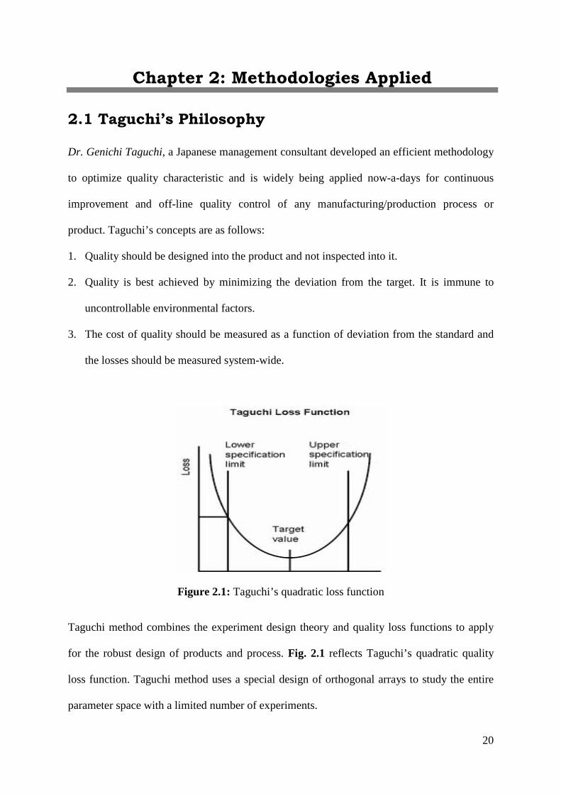
3. The cost of quality should be measured as a function of deviation from the standard and

the losses should be measured system-wide.

Figure 2.1: Taguchi’s quadratic loss function

Taguchi method combines the experiment design theory and quality loss functions to apply

for the robust design of products and process. Fig. 2.1 reflects Taguchi’s quadratic quality

loss function. Taguchi method uses a special design of orthogonal arrays to study the entire

parameter space with a limited number of experiments.

21

The change in the quality characteristic of a product responsive to a factor introduced in the

experimental design is termed as the Signal of the desired effect. The effect of the external

factors of the outcome of the quality characteristic under test is denoted as Noise. To use the

loss function as a figure of merit an appropriate loss function with its loss constant must be

established which is not always cost effective and easy. The experiment results are then

transformed into a Signal-to-Noise (S/N) ratio. Taguchi recommends the use of S/N ratio to

measure the quality characteristics deviating from the desired value. The S/N ratio for each

level of process parameters is computed based on the S/N analysis and converted into a single

metric. The aim in any experiment is to determine the highest possible S/N ratio for the result

irrespective of the type of the quality characteristics. A high value of S/N implies that signal

is much higher than the random effect of noise factors. In Taguchi method of optimization,

the S/N ratio is used as the quality characteristic of choice.

Taguchi’s techniques have been widely used in engineering design (Ross, 1996; Phadke,

1989). Taguchi’s approach to design of experiments is easy to be adopted and applied for

users with limited knowledge of statistics; hence it has gained a wide popularity in the

engineering and scientific community. The applications of Taguchi technique in the field of

materials processing and parametric optimization have been listed in references (Yang and

Tarng, 1998; Su et al., 1999; Nian et al., 1999; Lin, 2002; Davim, 2003; Ghani et al.,

2004).

According to Taguchi,

Quality characteristics are of three types as shown below.

1. Nominal-is-the-Best (NB) or Target-is-the-Best (TB)

2. Lower-the-Better (LB)

3. Higher-the-Better (HB)

22

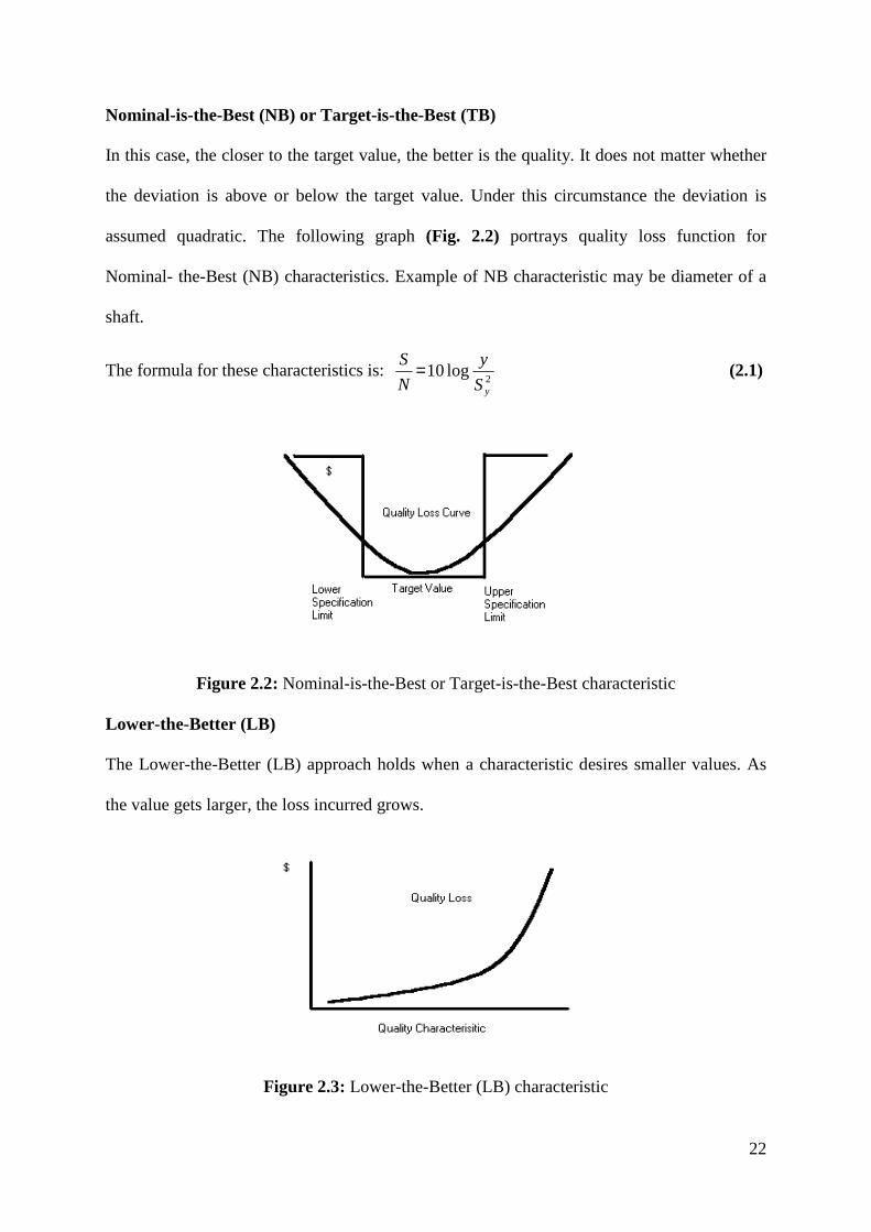
Nominal-is-the-Best (NB) or Target-is-the-Best (TB)

In this case, the closer to the target value, the better is the quality. It does not matter whether

the deviation is above or below the target value. Under this circumstance the deviation is

assumed quadratic. The following graph (Fig. 2.2) portrays quality loss function for

Nominal- the-Best (NB) characteristics. Example of NB characteristic may be diameter of a

shaft.

The formula for these characteristics is: 2

log10yS

y

N

S = (2.1)

Figure 2.2: Nominal-is-the-Best or Target-is-the-Best characteristic

Lower-the-Better (LB)

The Lower-the-Better (LB) approach holds when a characteristic desires smaller values. As

the value gets larger, the loss incurred grows.

Figure 2.3: Lower-the-Better (LB) characteristic

23

The formula for these characteristics is: ∑−= 21log10 y

nN

S (2.2)

The following graph (Fig. 2.3) portrays quality loss function for Lower-the-Better (LB)

characteristics. Example of LB characteristic is the amount of impurity in water.

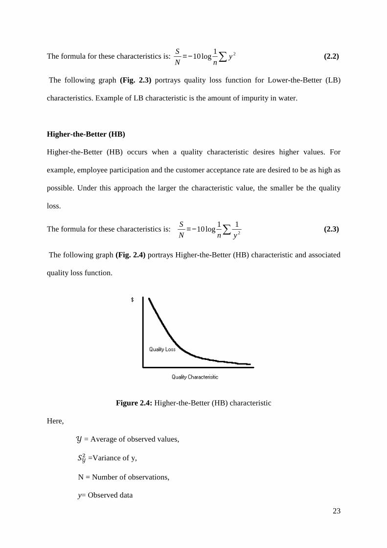
Higher-the-Better (HB)

Higher-the-Better (HB) occurs when a quality characteristic desires higher values. For

example, employee participation and the customer acceptance rate are desired to be as high as

possible. Under this approach the larger the characteristic value, the smaller be the quality

loss.

The formula for these characteristics is: ∑−=2

11log10

ynN

S (2.3)

The following graph (Fig. 2.4) portrays Higher-the-Better (HB) characteristic and associated

quality loss function.

Figure 2.4: Higher-the-Better (HB) characteristic

Here,

� = Average of observed values,

��� =Variance of y,

N = Number of observations,

y= Observed data

24

2.2 TOPSIS

TOPSIS (Technique for Order Preference by Similarity to Ideal Solution) method is very

popular and widely being used as a multi-attribute decision making (MADM) methodology

proposed by Hwang and Yoon (1981). The basic concept of this method is that the chosen

alternative should have the shortest distance from the positive ideal solution and the farthest

distance from negative ideal (anti-ideal) solution. Positive ideal solution is a solution that

maximizes the benefit criteria and minimizes cost criteria; whereas the negative ideal solution

maximizes the cost criteria and minimizes the benefit criteria. Tong and Su (1997)

highlighted that Taguchi's quadratic loss function and the indifference curve in the TOPSIS

method having similar features. The Taguchi method deals with a one-dimensional problem,

whereas TOPSIS method handles multi-dimensional problems. As a result, the relative

closeness computed in TOPSIS can be used as a performance measurement index for

optimizing multi-response problems in the Taguchi method. Liao, 2003; Wang and He

(2008) also applied TOPSIS for solving multi-response optimization problems. Following are

the procedural steps involved in TOPSIS method.

Step 1: This step involves development of initial decision-making matrix. The row of this

matrix is allocated to one alternative; each column corresponds to one attribute values for

various alternatives. The decision making matrix can be expressed as:

=

mnmjmm

ijii

nj

nj

m

i

xxxx

xxx

xxxx

xxxx

A

A

A

A

.

.....

..

.....

.

.

.

.

21

21

222221

111211

2

1

D (2.4)

Here, iA ( ).......,,2,1( mi = represents the possible alternatives; ( )njx j ........,,2,1= represents

the attributes relating to alternative performance, nj .,,.........2,1= and ijx is the performance

25

of iA with respect to attribute .jX

Step 2: Obtain the normalized decision matrix ijr .This can be represented as:

∑=

=m

iij

ijij

x

xr

1

2

(2.5)

Here, ijr represents the normalized performance of iA with respect to attribute .jX

Step 3: obtain the weighted normalized decision matrix, [ ]ijv=V can be found as:

ijj rwV = (2.6)

Here, ∑=

=n

jjw

1

1

Step 4: Determine the ideal (best) and negative ideal (worst) solutions in this step. The ideal

and negative ideal solution can be expressed as:

a) The ideal solution:

( ) ( ){ }miJjvJjvA iji

iji

,..........,2,1min,max ' =∈∈=+ (2.7)

{ }++++= nj vvvv ,.....,........,, 21

b) The negative ideal solution:

( ) ( ){ }miJjvJjvA iji

iji

........,,2,1max,min ' =∈∈=− (2.8)

{ }−−−−= nj vvvv ,....,........,, 21

Here,

{ }:,.......,2,1 jnjJ == Associated with the beneficial attributes

{ }:,.......,2,1' jnjJ == Associated with non beneficial adverse attributes

Step 5: Determine the distance measures. The separation of each alternative from the ideal

solution is given by n-dimensional Euclidean distance from the following equations:

26

( )∑=

++ −=n

jjiji vvS

1

, mi .........,,2,1= (2.9)

( )∑=

−− −=n

jjiji vvS

1

, mi .........,,2,1= (2.10)

Step 6: Calculate the relative closeness (also called closeness coefficient, CC) to the ideal

solution:

10;,,.........2,1, ≤≤=+

= +−+

−+

iii

ii Cmi

SS

SC (2.11)

Step 7: Rank the preference order. The alternative with the largest relative closeness is the

best choice.

In the present study +iC for each experimental run has been termed as Multi-Performance

Characteristic Index (MPCI) which has been optimized by Taguchi method.

2.3 Principal Component Analysis (PCA)

Data preprocessing is the first step in Principal Component Analysis (PCA) which transfers

original data sequence to a comparable sequence. PCA is a multivariate statistical approach,

which allows the representation of the original database into a new reference system

characterized by new variables called principal components (PCs). Each PC has the property

of explaining the maximum possible amount of variance obtained in the original dataset. The

PCs, which are expressed as linear combinations of the original variables, are orthogonal to

each other and can be used for effective representation of the system under investigation,

with a lower number of variables in the new system of variables being called scores, while

the coefficient of linear combination describes each PCs, i.e. the weight of original variables

of each PC. To avoid any influence on the optimization of the machining process from the

27

units used for evaluating the MPCs, normalization of the data required, in order to provide

information for determining the optimal levels of process parameters.

The normalization is taken by the following Equations.

1) For Lower-the-Better (LB) criterion

( ) ( ) ( )( )[ ] ( ) ,

minmax

maxˆ

kxkx

kxkxkx

ikik

iiki −

−=

(2.12)

2) For Higher-the-Better (HB) criterion

( ) ( )( )[ ] ( ) ,

minmax

minˆ

kxkx

kxxkx

ikik

ikii −

−=

(2.13)

Here, ( )kx i denotes the value after normalization for the thk quality characteristic value,

( )kx i is the experimental data of thk quality characteristic duringthi experiment.

The obtained data may have a number of variables and there may be some redundancy

(correlation) among those variables. To get rid of such correlation, it is possible to reduce a

set of observed variables into a smaller set of new variables called principal components.

Principal components analysis is a method that reduces data dimensionality by performing a

covariance/correlation analysis between factors and linear combination of optimally-weighted

observed variables. Factor analysis is used to summarize the data structure in a few

dimensions of the data and also explain the dimensions associated with large data variability.

An orthogonal rotation simply rotates the axes to give a different perspective. The different

methods are Equimax, Varimax, Quartimax, and Orthomax. A parameter, gamma is

determined during the rotation method. If the method with a low value of gamma is used, the

rotation will tend to simplify the rows of the loadings and if the method with a high value of

gamma is used the rotation will tend to simplify the columns of the loadings. Varimax

rotation is used because it maximizes the variance of the squared loadings.

28

PCA is a way of identifying patterns in the correlated data, and expressing the data in such a

way so as to highlight their similarities and dissimilarities/differences. The main advantage of

PCA is that once the patterns in data have been identified, the data can be compressed, i.e. by

reducing the number of dimensions, without much loss of information. PCA is an efficient

statistical technique while studying multi-quality characteristics, those are highly correlated.

The PCA allows data which contain information of multi-quality characteristics to be

converted into several independent quality indicators. Part of these indicators is then selected

to construct a composite quality indicator, which is the representative of multi-quality

features of the process output. The methods involved in PCA are discussed below:

1. Getting some data

2. Normalization of data

3. Calculation of covariance/correlation matrix.

4. Interpretation of covariance/correlation matrix.

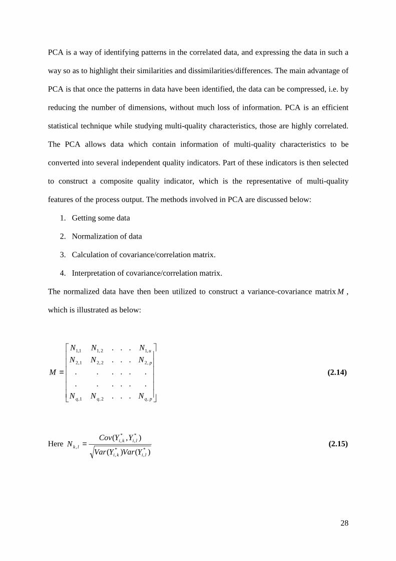
The normalized data have then been utilized to construct a variance-covariance matrixM ,

which is illustrated as below:

=

pqqq

p

u

NNN

NNN

NNN

M

,2,1,

,22,21,2

,12,11,1

...

......

......

...

...

(2.14)

Here )()(

),(*,

*,

*,

*,

,

liki

likilk

YVarYVar

YYCovN = (2.15)

29

In which u stands for the number of quality characteristics and p stands for the number of

experimental runs. Then, eigenvectors and Eigen values of matrix M can be computed, which

are denoted byjV and jλ respectively.

In PCA the eigenvector jV represents the weighting factor of j number of quality

characteristics of the jth principal component. For example, if jQ represents the jth

quality characteristic, the jth principal component jψ can be treated as a quality indicator

with the required quality characteristic.

QVQVQVQV jjjjjjj'

2211 ........................ =+++=ψ (2.16)

It is to be noted that every principal component jψ represents a certain degree of

explanation of the variation of quality characteristics, namely the accountability proportion

(AP). When several principal components are accumulated, it increases the accountability

proportion of quality characteristics. This is denoted as cumulative accountability proportion

(CAP). The composite principal component ψ may be defined as the sum/ linear

combination of principal components with their individual Eigen values. Thus, the composite

principal component represents the overall quality indicator as shown below:

∑=

=k

jj

1

ψψ (2.17)

If a quality characteristic jQ strongly dominates in the jth principal component, this

principal component becomes the major indicator of such a quality characteristic. It should be

noted that one quality indicator may often represent all the multi-quality characteristics.

Selection of individual principal components (jψ ), those to be included in the composite

quality indicatorψ , depends on their individual accountability proportion. Application of

PCA has been found in the work carried out by (Su and Tong, 1997; Datta et al., 2009b;

Routara et al., 2010).

30

2.4 Utility Theory

There are always more than one quality responses (or output characteristics) in product/

process design and it is often required to choose an optimum parameter combination for these

responses simultaneously. Taguchi method, as a cost-effective method for off-line quality

control, has been widely employed by quality engineering to deal with single-response

problem, but fails to solve multi-objective optimization problem. In order to overcome this,

utility theory (Walia et al., 2006; Datta et al., 2006) have been applied by previous

investigators in combination with Taguchi method. The methodological basis for utility

approach is to transform the estimated response of each quality characteristic into a common

index. It is the measure of effectiveness of an attribute (or quality characteristics) and there

are attributes evaluating the outcome space, then the joint utility function can be expressed

as:

))(.......,),........(),(().......,,.........( 22112,1 nnn XUXUXUfXXXU = (2.18)

The overall utility function is the sum of individual utilities if the attributes are independent,

and is given as follows:

∑=

=n

iiin XUXXXU

12,1 )().......,,.........(

(2.19)

The overall utility function after assigning weights to the attributes can be expressed as:

∑=

⊗=n

iiiin XUWXXXU

12,1 )().......,,.........(

(2.20)

The preference number can be expressed on a logarithmic scale as follows:

×=

'log

i

ii X

XAP

(2.21)

Here,

iX is the value of any quality characteristic or attribute i

31

'iX is just acceptable value of quality characteristic or attribute i and A is a constant. The

value A can be found by the condition that if *XX i = (where *X is the optimal or best value),

then .9=iP Therefore,

'

*

log

9

iX

XA = (2.22)

The overall utility can be expressed as follows:

i

n

ii PWU ⊗=∑

=1 (2.23)

Subject to the condition:

11

=∑=

n

iiW

(2.24)

Overall utility index generally servers as the single objective function for optimization.

Among various quality characteristics types, viz. Lower-the-Better (LB), Higher-the-Better

(HB), and Nominal-the-Best (NB) suggested by Taguchi, the utility function would be

Higher-the-Better type. Therefore, if the quality function is maximized, the quality

characteristics considered for its evaluation would automatically be optimized (maximized or

minimized as the case may be).

2.5 Desirability Function

Desirability function approach was first proposed by Derringer and Suich (1980). In

desirability function approach, individual responses are transformed to corresponding

desirability values. Desirability value depends on acceptable tolerance range as well as target

of the response. Unity is assigned, as the response reaches its target value, which is the most

desired situation. If the value of the response falls beyond the prescribed tolerance rage,

which is not desired, its desirability value is assumed as zero. Therefore, desirability value

may vary from zero to unity.

There are three different types of desirability

1. Higher-the-Better (HB)

2. Lower-the-Better (LB)

3. Nominal-the-Best (NB)

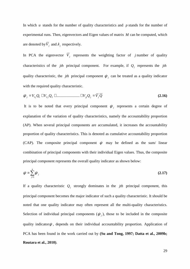
Higher-the-Better (HB)

Desirability function corresponding to

Fig. 2.5. The value ofy is expected to be the high. When

according to the requirement, the desirability value

criteria value, i.e. less than the acceptable limit, the desirability value equals to 0. The

desirability function of the Higher

given in Eqs (2.25-2.27). Here

the upper tolerance limit ofy

assigned previously according to the consideration of the

Figure 2.5

which is not desired, its desirability value is assumed as zero. Therefore, desirability value

ferent types of desirability characteristics.

function corresponding to Higher-the-Better (HB) criterion ha

is expected to be the high. Wheny exceeds a particular criteria value,

according to the requirement, the desirability value id equals to 1; ify is less than a particular

a value, i.e. less than the acceptable limit, the desirability value equals to 0. The

desirability function of the Higher-the-Better (HB) criterion can be written in the form as

Here miny denotes the lower tolerance limit ofy , the

andr represents the desirability function index, which is to be

ording to the consideration of the decision-maker.

Figure 2.5: Desirability function (Higher-the-Better)

32

which is not desired, its desirability value is assumed as zero. Therefore, desirability value

has been shown in

exceeds a particular criteria value,

is less than a particular

a value, i.e. less than the acceptable limit, the desirability value equals to 0. The

etter (HB) criterion can be written in the form as

, the maxy represents

represents the desirability function index, which is to be

,ˆ minyy ≤ 0=id

,ˆ maxmin yyy ≤≤

r

i yy

yyd

−−

=minmax

minˆ

maxˆ yy ≥ , 1=id

Lower-the-Better (LB)

The desirability function corresponding to

Fig. 2.6. The value ofy is expected to be

criteria value, the desirability value

desirability value equals to 0.

the Lower-the-Better (LB) criterion can be written as below in

denotes the lower tolerance limit of

represents the desirability function index, which is to be assigned previously according to the

consideration of the decision-maker

Figure 2.6

function corresponding to Lower-the-Better (LB) criterion

is expected to be as less as possible. Wheny is less than a particular

criteria value, the desirability valueid equals to 1; ify exceeds a particular criteria value, the

desirability value equals to 0. If id varies within the range (0, 1). The desirability function of

etter (LB) criterion can be written as below in Eqs. (2.28

denotes the lower tolerance limit ofy , the maxy represents the upper tolerance l

represents the desirability function index, which is to be assigned previously according to the

maker.

Figure 2.6: Desirability function (Lower-the-Better)

33

(2.25)

(2.26)

(2.27)

etter (LB) criterion has been shown in

is less than a particular

exceeds a particular criteria value, the

The desirability function of

2.28-2.30). Here miny

represents the upper tolerance limit of y andr

represents the desirability function index, which is to be assigned previously according to the

34

,ˆ minyy ≤ 1=id (2.28)

,ˆ maxmin yyy ≤≤

r

i yy

yyd

−−

=maxmin

maxˆ

(2.29)

maxˆ yy ≥ , 0=id (2.30)

Nominal-the-Best (NB)

The values ofy are required to achieve a particular targetT as shown in Fig. 2.7. When y

equals toT , the desirability value equals to 1; if the departure ofy exceeds a particular range

from the target, the desirability value equals to 0, and such situation represents the worst case.

The desirability function for the Nominal-the-Best (NB) can be written as given in Eqs.

(2.31-2.32).

,ˆmin Tyy ≤≤

r

i yT

yyd

−−

=min

minˆ

(2.31)

,ˆ maxyyT ≤≤

r

i yT

yyd

−−

=max

maxˆ

(2.32)

Here,

maxy and miny represent the upper/lower tolerance limits ofy andr represent the desirability

function index.

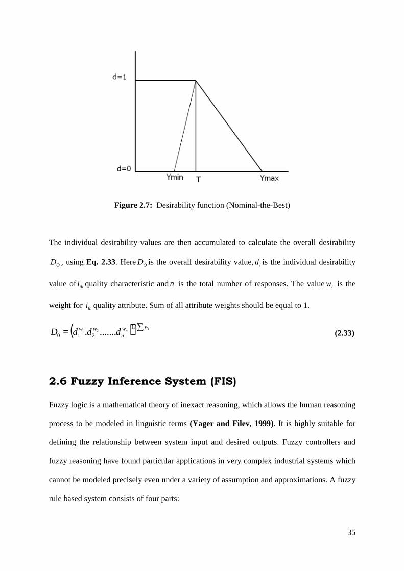
Figure 2.7

The individual desirability values

OD , using Eq. 2.33. Here OD

value of thi quality characteristic

weight for thi quality attribute. Sum of all attribute weights should be equal to 1.

( ) ∑= nww

nww dddD

/1

210 ........ 21

2.6 Fuzzy Inference System (FIS)

Fuzzy logic is a mathematical theory of inexact reasoning, which allows the human reasoning

process to be modeled in linguist

defining the relationship between system input and desired outputs. Fuzzy controllers and

fuzzy reasoning have found particular applications in very complex industrial systems which

cannot be modeled precisely even under a variety of assumption and approximations.

rule based system consists of four parts:

Figure 2.7: Desirability function (Nominal-the-Best)

The individual desirability values are then accumulated to calculate the overall desirability

O is the overall desirability value,id is the individual desirability

quality characteristic andn is the total number of responses. The value

attribute. Sum of all attribute weights should be equal to 1.

iw

2.6 Fuzzy Inference System (FIS)

Fuzzy logic is a mathematical theory of inexact reasoning, which allows the human reasoning

process to be modeled in linguistic terms (Yager and Filev, 1999). It is highly suitable for

defining the relationship between system input and desired outputs. Fuzzy controllers and

fuzzy reasoning have found particular applications in very complex industrial systems which

precisely even under a variety of assumption and approximations.

rule based system consists of four parts:

35

accumulated to calculate the overall desirability

is the individual desirability

The value iw is the

attribute. Sum of all attribute weights should be equal to 1.

(2.33)

Fuzzy logic is a mathematical theory of inexact reasoning, which allows the human reasoning

It is highly suitable for

defining the relationship between system input and desired outputs. Fuzzy controllers and

fuzzy reasoning have found particular applications in very complex industrial systems which

precisely even under a variety of assumption and approximations. A fuzzy

36

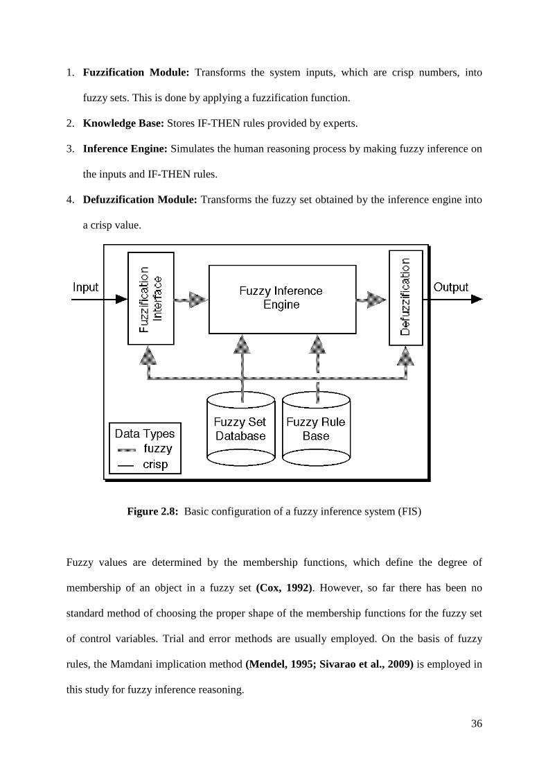
1. Fuzzification Module: Transforms the system inputs, which are crisp numbers, into

fuzzy sets. This is done by applying a fuzzification function.

2. Knowledge Base: Stores IF-THEN rules provided by experts.

3. Inference Engine: Simulates the human reasoning process by making fuzzy inference on

the inputs and IF-THEN rules.

4. Defuzzification Module: Transforms the fuzzy set obtained by the inference engine into

a crisp value.

Figure 2.8: Basic configuration of a fuzzy inference system (FIS)

Fuzzy values are determined by the membership functions, which define the degree of

membership of an object in a fuzzy set (Cox, 1992). However, so far there has been no

standard method of choosing the proper shape of the membership functions for the fuzzy set

of control variables. Trial and error methods are usually employed. On the basis of fuzzy

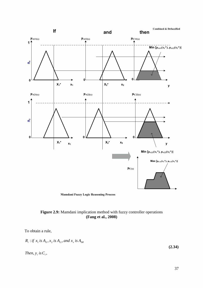
rules, the Mamdani implication method (Mendel, 1995; Sivarao et al., 2009) is employed in

this study for fuzzy inference reasoning.

37

µA11(x) µA12(x) µC11(x)

µA21(x) µA22(x) µC22(x)

0 0 0

0 0 0

1

1

X1* x1 X2* x2 y

X1* x1X2* x2 y

If and then

Mamdani Fuzzy Logic Reasoning Process

Min [µA21(x1*), µA22(x2*)]

Min [µA11(x1*), µA12(x2*)]

Combined & Defuzzified

Max [µC11(x1*), µC12(x2*)]

µC(x)

Figure 2.9: Mamdani implication method with fuzzy controller operations (Fang et al., 2008)

To obtain a rule,

,,

,,: 2211

ii

iMsiii

CisyThen

AisxandAisxAisxifR

(2.34)

38

Here M is the total number of fuzzy rules. ),,.........,2,1( sjx j = are the input variables,iy are

the output variables and iij andCA are fuzzy sets modeled by the membership functions

)( jAij xµ and )( iCi yµ , respectively. Based on the Mamdani implication method of inference

reasoning for a set of disjunctive rules, the aggregated output for the M rules is

[ ]{ },)(),......,(),(minmax)( 2211 sAisAiAijCi xxxy µµµµ = Mi ,........,2,1= (2.35)

Elements of a Fuzzy Inference System (FIS) have been shown in Fig. 2.8. The above

equation is illustrated in Fig. 2.9. The graph represents the fuzzy reasoning process for two

rules, R1 and R2, with two input variables which are triangle shaped membership functions.

Using a defuzzification method, fuzzy values can be combined into one single crisp output

value. The centre of gravity, one of the most popular methods for defuzzifying fuzzy output

functions, is employed in this study. The formula to find the centroid of the combined outputs

iy is given by:

∫∫=

dyy

dyyyy

ici

icii

i)(

)(ˆ

µ

µ (2.36)

2.7 Adaptive Neuro-Fuzzy Inference System (ANFIS)

Adaptive Neuro-fuzzy inference system is a fuzzy inference system implemented in the

framework of an adaptive neural network. By using a hybrid learning procedure, ANFIS can

construct an input-output mapping based on both human-knowledge as fuzzy if-then rules

and stipulated input-output data pairs for neural networks training. ANFIS architecture has

been shown in Fig. 2.10. Five network layers are used by ANFIS to perform the following

fuzzy inference steps: (i) Input Fuzzification, (ii) Fuzzy Set Database Construction, (iii)

Fuzzy Rule Base Construction, then (iv) Decision-Making and (v) Output Defuzzification.

Learning or training phase of a neural network is a process to determine parameter values to

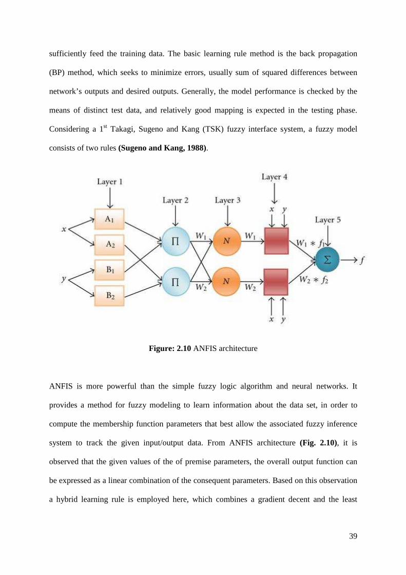
39

sufficiently feed the training data. The basic learning rule method is the back propagation

(BP) method, which seeks to minimize errors, usually sum of squared differences between

network’s outputs and desired outputs. Generally, the model performance is checked by the

means of distinct test data, and relatively good mapping is expected in the testing phase.

Considering a 1st Takagi, Sugeno and Kang (TSK) fuzzy interface system, a fuzzy model

consists of two rules (Sugeno and Kang, 1988).

Figure: 2.10 ANFIS architecture

ANFIS is more powerful than the simple fuzzy logic algorithm and neural networks. It

provides a method for fuzzy modeling to learn information about the data set, in order to

compute the membership function parameters that best allow the associated fuzzy inference

system to track the given input/output data. From ANFIS architecture (Fig. 2.10), it is

observed that the given values of the of premise parameters, the overall output function can

be expressed as a linear combination of the consequent parameters. Based on this observation

a hybrid learning rule is employed here, which combines a gradient decent and the least

40

squares method to determine a feasible of antecedent and consequent parameters (Jang1991;

Jang 1993).

ANFIS on-line identification of a characteristic feature starts by obtaining the data set (input-

output data pairs) and dividing it into training and checking or validating data sets. The

training data set is used to find the initial premise parameters for the fuzzy membership

functions by equally spacing each membership function. The values of the premise

parameters are fixed, so the overall on-line predicted characteristic feature under

consideration can be expressed as a linear combination of consequent parameters.

The Sugeno fuzzy model (Jang and Sun, 1995) describes the ANFIS architecture and its

learning algorithm. The fuzzy inference system has two inputsm andn and one outputf . For

a first-order Sugeno fuzzy model, a typical rule set with two fuzzy IF–THEN rules can be

expressed as:

Rule 1: 111111 )()( rnqmpfthenBisnandAismif ++= (2.37)

Rule 2: 222222 )()( rnqmpfthenBisnandAismif ++= (2.38)

Here, 212121 ,,,, randrqqpp are linear parameters, and 2121 ,, BandBAA are non linear

parameters.

The corresponding equivalent ANFIS architecture has been shown in Fig. 2.10. The entire

system architecture consists of five layers, namely, a fuzzy layer, a product layer, a

normalized layer, a defuzzy layer and a total output layer. The following section discussed

the relationship between the output and input of each layer in the ANFIS.

Layer 1 is the fuzzy layer, in whichm andn are the input of nodes 2121 ,, BandBAA

respectively. 2121 ,, BandBAA are the linguistic labels used in the fuzzy theory for dividing

the membership functions. The membership relationship between the output and input

functions of this layer can be expressed as:

41

)2,1()(

)2,1()(

,1

,1

==

==

jnO

imO

Bjj

Aii

µµ

(2.39)

Here iO ,1 and jO ,1 denote the output functions and Aiµ and Bjµ denote the membership

functions.

Layer 2 is the product layer that consists of two nodes labeled asΠ . The output 1w and 2w

are the weight functions of the next layer. The output of this layer is the product of the input

signal, which is defined as follows:

)2,1()()(,2 === inmwO BiAiii µµ (2.40)

Here, iO ,2 denotes the output of Layer 2.

The third layer is the normalized layer, whose nodes are labeled N. Its function is to

normalize the weight function in the following process:

)2,1(21

,3 =+

== iww

wwO i

i (2.41)

Here, iO ,3 denotes the layer 3 output.

The fourth layer is the defuzzy layer, whose nodes are adaptive. The output equation is

),( rqnpmw ++ where iii randqp , denote the linear parameters or so-called consequent

parameters of the node. The defuzzy relationship between the input and output of this layer

can be de fined as:

)2,1()(,4 =++== irnqmpwfwO iiiiiii (2.42)

Here, iO ,4 denotes the Layer 4 output.

The fifth layer is the total output layer, whose node is labeled as∑ . The output of this layer is

the total of the input signals, which represents the tool-state (normal or failure) detection

result. The results can be written as:

42

)2,1(,5 ===∑∑

∑ iw

fwfwO

ii

iiiii ii (2.43)

Here, iO ,5 denotes the Layer 5 output.

43

Chapter 3

Application of TOPSIS based Taguchi Method

3.1 Coverage

Quality and productivity are the two major parameters of concern for every manufacturing or

production unit in order to achieve high quality product towards fulfillment of the need and

satisfaction of the customers in an economic way. In this globalization era, there are more than

one product quality assessment factors that lead to competition in the marketplace. So the main

goal is to find the optimum solution to satisfy customers’ multiple needs of the product

performance in an economic cost.

Glass fiber reinforced polymer (GFRP) comprises high strength to weight ratio, toughness,

excellent corrosion and thermal resistance. Due to its excellent properties over other engineering

materials GFRP composite is being applied in defence, aerospace engineering, civil engineering

and automobile engineering as well. Due to widespread upcoming applications of GFRP

composites; machining and machinability aspects of composites have become the major concern

of the industrialists as well as academicians. During production process, the main concern is to

produce a specified surface texture because it depends on the various input parameters selected

during operation. A small change in the machining parameters seemed to impose significant

effect on the surface produced. Therefore, optimization of machining parameters is the major

issue to enhance product quality as well as overall performance of the said process.

In this chapter, TOPSIS technique has been integrated with Taguchi’s philosophy towards

solving multi-objective optimization problem in machining of composites as a case study. The

44

following paragraph describes some of the important investigations carried out by pioneers

towards successful implementation of TOPSIS method.

Hwang and Yoon (1981) classified the multi-attribute decision making (MADM) problem on

the basis of the type of information of the decision maker and the salient features of the

information. The authors described TOPSIS as the suitable method due to information given in

cardinal preferences of the attributes. Lan (2009) proposed a multi objective integration

technique using orthogonal array and TOPSIS technique to optimize the precision CNC turning

conditions. The optimum multi-objective cutting parameters were achieved by analysis of factor

responses in the Taguchi experiment. Yang and Chou (2005) assumed the control factors as a

discrete value by which Taguchi quality loss function were adapted to solve the mean and

variance effects. Further TOPSIS method was used to find the replaced objective function for the

multiple responses and also assessed the distance from the positive and negative ideal solution of

each alternative. Angun et al. (2003) solved the multi response problem by choosing one

response as objective and remaining as constraints. The search direction was scaled and project

estimated steepest-descent direction called the estimated affine scaling search direction. Tong

and Su (1997) adopted a MADM method a technique for order preference by similarity to ideal

solution (TOPSIS) to optimize the multi-response robust design problem. They considered the

sampling variability of each response by the Taguchi quality loss function. Wang and He (2007)

reported that in conventional TOPSIS method, responses were usually transformed into quality

loss, and then normalized by the largest quality loss which was not suitable for Nominal-the-Best

(NB) problem. So, modified method was proposed based on the TOPSIS and made an

improvement to adapt a nominal the best responses. Liu (2011) provided an extended method of

45

TOPSIS in which attributes values and priority weight took the form of generalized interval

valued trapezoidal fuzzy number (GIVTFN).

Literature survey (described in Chapter 1) reveals that traditional methods are very

straightforward (consisting of a number of assumptions) and not free from limitations. It is

seemed that TOPSIS method adapted from Multi-Criteria Decision Making (MCDM) combined

with Taguchi method has not been applied before in the field of composite machining. Moreover,

most of the studies concentrated on optimizing average surface roughness (Ra) only. But there

exist a number of surface roughness parameters of statistical importance which need to be

investigated in detail. In this context, the study explores application of TOPSIS based MCDM

combined with Taguchi method (Yang and Tang, 1998) for parametric optimization in

machining of glass fiber reinforced polyester composites while considering multiple surface

roughness characteristics of the machined work piece. The detailed description of the

methodology followed by application feasibility has been described in later part.

3.2 Experimentation

The multi-criteria based optimization of the machining (turning) process for GFRP composites is

primarily concentrated towards optimizing the process conditions to obtain the least extent of a

set of surface roughness characteristics of the machinated surface. There are multiple surface

roughness characteristics (Ra, Rz, Rt, Rsm, Rku, Rz1max etc.) of statistical importance. Different

surface roughness characteristics are used in different convention systems in different countries.

The objective of the thesis is to find out a practical optimization problem consisting of mutually

correlated response features (output measure). Aforesaid multiple roughness features are

correlated to each other and greatly influenced by the process control parameters. In order to

46

achieve high surface finish, all these parameters need to be optimized (minimized)

simultaneously. It is true that in general, the surface roughness of a machined surface is simply

evaluated by finding out the corresponding Ra value in almost all topical literature. However, the

following are the references (Davim and Mata, 2005; Palanikumar et al., 2008; Palanikumar,

2008a) in which pioneer researchers pointed out the importance of simultaneous consideration of

multiple roughness features. Motivated by this, the study has been planned to consider correlated

multiple surface roughness characteristics in the list of objective functions for the said composite

machining.

The present study has been done through the following plan of experiments.

A. Checking and preparing the centre lathe ready for performing the machining operation.

B. Cutting GFRP bars and performing initial turning operation in lathe to get desired

dimension ( 15050×φ ) of the work pieces.

C. Performing straight turning operation on specimens in various cutting environments

involving various combinations of process control parameters like spindle speed, feed

and depth of cut.

D. Measuring surface roughness parameters with the help of a portable stylus-type

profilometer, Talysurf (Taylor Hobson, Surtronic 3+, UK).

Glass fiber (E-glass-R099 1200 P556) reinforced Polyester composite has been selected as work

piece material. The specifications of the work piece material have been shown in Table 3.1. The

ISO specification of the tool holder used for the turning operation is a WIDAX tool holder PC

LNR 2020 K12 and the tool insert used for the study are carbide K-20, (CNMA 120408).

In the present study, spindle speed (N, RPM), feed rate (f, mm/min) and depth of cut (d, mm),

have been selected as design factors while other parameters have been assumed to be constant

47

over the experimental domain. The process variables (design factors) with their values at

different levels have been listed in Table 3.2. It is known that the selection of the values of the

variables is limited by the capacity of the machine used in the experimentation as well as the

recommended specifications for different work piece and tool material combinations. Therefore,

three levels have been selected for each of the aforesaid three factors. In the present

investigation, Taguchi’s L9 orthogonal array (OA) design (without factorial interaction) has been

considered for experimentation (Table 3.3). The machine used for turning is PINACHO lathe

(specifications have been included at the end of this chapter). The surface roughness parameters

have been measured using the stylus-type profilometer, Talysurf (Taylor Hobson, Surtronic 3+).

The values of measured roughness parameters: (average of two trials) Rq, Ra, Rt, Rku, Rz, Rsm

have been shown in Table 3.4 with pictorial representations of surface profile shown in at the

end of this thesis (Appendix 1). The definitions of aforesaid surface roughness parameters along

with MRR have also been included at the end of this thesis (Appendix 2).

It is widely accepted in most of the manufacturing process optimization that experimental

designs based on Taguchi’s Orthogonal Array (OA) is used a starting point since it allows the

identification of the interaction effects of independent variables on the responses. A full factorial

design of experiment represents all parametric combinations. As number of factors and their

levels of variation increase; the total number of experimental run in full-factorial design of

experiment exponentially increases. This results in consumption of excessive time and cost.

Taguchi philosophy adopts OA to reduce experimentation time and cost. Without conducting

large set of experiments; only a limited number of experiments are required for reliable

prediction of the optimal. Therefore, adaptation of L9 OA instead of full-factorial design of

experiment is fully justified.

48

3.3 Numerical Illustrations

The methodology adopted for solution of multi-response optimization problem has been

summarized in a block diagram shown at the end of this thesis (Appendix 3). Six output responses

related to various surface roughness parameters has been taken as criteria attributes with nine

alternatives (process environments). Taguchi’s loss function in the form of S/N ratio has been

calculated to account for the mean and variability of each response. For all the surface roughness

parameters, S/N ratio has been calculated based on Lower-the-Better (LB) criteria (Eq. 3.1).

−= ∑=

n

iiy

nNS

1

21log10/ (3.1)

Here,n is the number of measurements, andiy the measuredthi characteristic value i.e. thi quality

indicator.

Calculated S/N ratios have been shown in Table 3.5. The normalized S/N ratios have been

computed using Eq. 2.5 of Chapter 2 and shown in Table 3.6.

The next step is to calculate the weight of each attributes by the Standard Deviation Method

(SDM) to calculate the weighted normalized rating using Eq. 3.2. The calculated weighted

normalized S/N ratio values are shown in Table 3.7.

The standard deviation method calculates objective weights of the attributes (Eq. 3.2).

∑=

=M

kkjjw

1

/ σσ (3.2)

Here, jσ is the standard deviation of the normalized vectorijr .

The standard deviation method calculates the objective weights of the attributes without giving

any consideration to the preferences of the decision maker. The set of factor weight for each

49

surface roughness is w1 = 0.204213, w2 = 0.104796, w3 = 0.199887, w4 = 0.100424, w5 =

0.141389, w6 = 0.249292. The next step is to calculate the ideal (best) and negative ideal (worst)

solution i.e. A+ and A- (using Eqs. 2.7-2.8 of Chapter 2) and shown in Table 3.8. The distance

measures i.e. −+ii SS , (separation distance of each alternative from the ideal one) have been

determined by using (Eqs. 2.9-2.10 of Chapter 2). Then calculated distance measures have been

shown in Table 3.9. Finally, the similarity to ideal solution for each scenario of alternative+iC

has been obtained by Eq. 2.11 of Chapter 2 (shown in Table 3.10). This +iC has been treated as

MPCI of the surrogate responses for the proposed multi-response simulation-optimization

problem. The alternative with the largest relative closeness is said to be the best choice and made

in descending order according to the preference value. The best preference has been determined

by optimizing (maximizing) MPCI in Taguchi method. Fig. 3.1 represents optimal parametric

combination (N3 f2 d3) evaluated from mean S/N ratio plot for MPCI. Optimal result has been

validated by satisfactory confirmatory test. Predicted value of S/N ratio of MPCI becomes -

1.55809 (highest among all entries of MPCIs SN ratio in Table 3.10). In confirmatory

experiment the value came -1.4367. So, quality has improved using the said optimal setting.

Table 3.11 represents mean values table of S/N ratios of MPCIs. The degree of influence of

various factors on MPCI can be estimated from this analysis. It shows that feed rate is the most

significant factor on influencing MPCIs following with depth of cut and spindle speed.

3.4 Concluding Remarks

This chapter presents an integrated optimization philosophy using TOPSIS concept combined

with Taguchi method for optimizing multiple surface roughness parameters optimization in

50

machining of GFRP composites. The study illustrates the effectiveness of the proposed method

as well. The analysis in this chapter exposes that Taguchi’s quadratic loss function and TOPSIS

concept can be efficiently integrated towards a flexible compatible multi-response optimization

methodology. The traditional Taguchi method deals with one dimensional problem (single

response), while TOPSIS is capable of dealing with multi dimensional problem (multiple criteria

attribute). By exploring TOPSIS concept multiple criterions can be logically aggregated to

convert a single performance index (MPCI). MPCI can easily be optimized to determine the

optimal process environment which facilitates in mass production and consequently product

quality improvement.

However, the procedure reported in the preceding sections is not free from limitations. The

drawbacks have been enlisted herewith.

1. In this procedure response correlation has not been considered.

2. Individual response weight computed from statistical analysis of experimental data

(standard deviation) does not provide accurate degree of response importance in reality.

Also it depends on the type of data gathered through experiments.

In order to bypass uncertainty in appropriate assignment of response weights; next chapter

explores the concept of fuzzy logic followed by development and subsequent execution of a

Fuzzy Inference System (FIS) in order to aggregate multiple performance characteristics (output

responses) into a single performance measure. This equivalent unique performance measure has

been optimized (maximized) by Taguchi method.

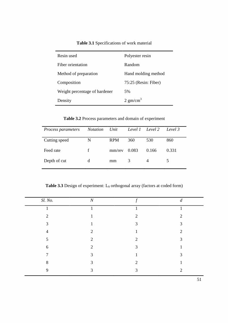
51

Table 3.1 Specifications of work material

Resin used Polyester resin

Fiber orientation Random

Method of preparation Hand molding method

Composition 75:25 (Resin: Fiber)

Weight percentage of hardener 5%

Density 2 gm/cm3

Table 3.2 Process parameters and domain of experiment

Process parameters Notation Unit Level 1 Level 2 Level 3

Cutting speed N RPM 360 530 860

Feed rate f mm/rev 0.083 0.166 0.331

Depth of cut d mm 3 4 5

Table 3.3 Design of experiment: L9 orthogonal array (factors at coded form)

Sl. No. N f d

1 1 1 1

2 1 2 2

3 1 3 3

4 2 1 2

5 2 2 3

6 2 3 1

7 3 1 3

8 3 2 1

9 3 3 2

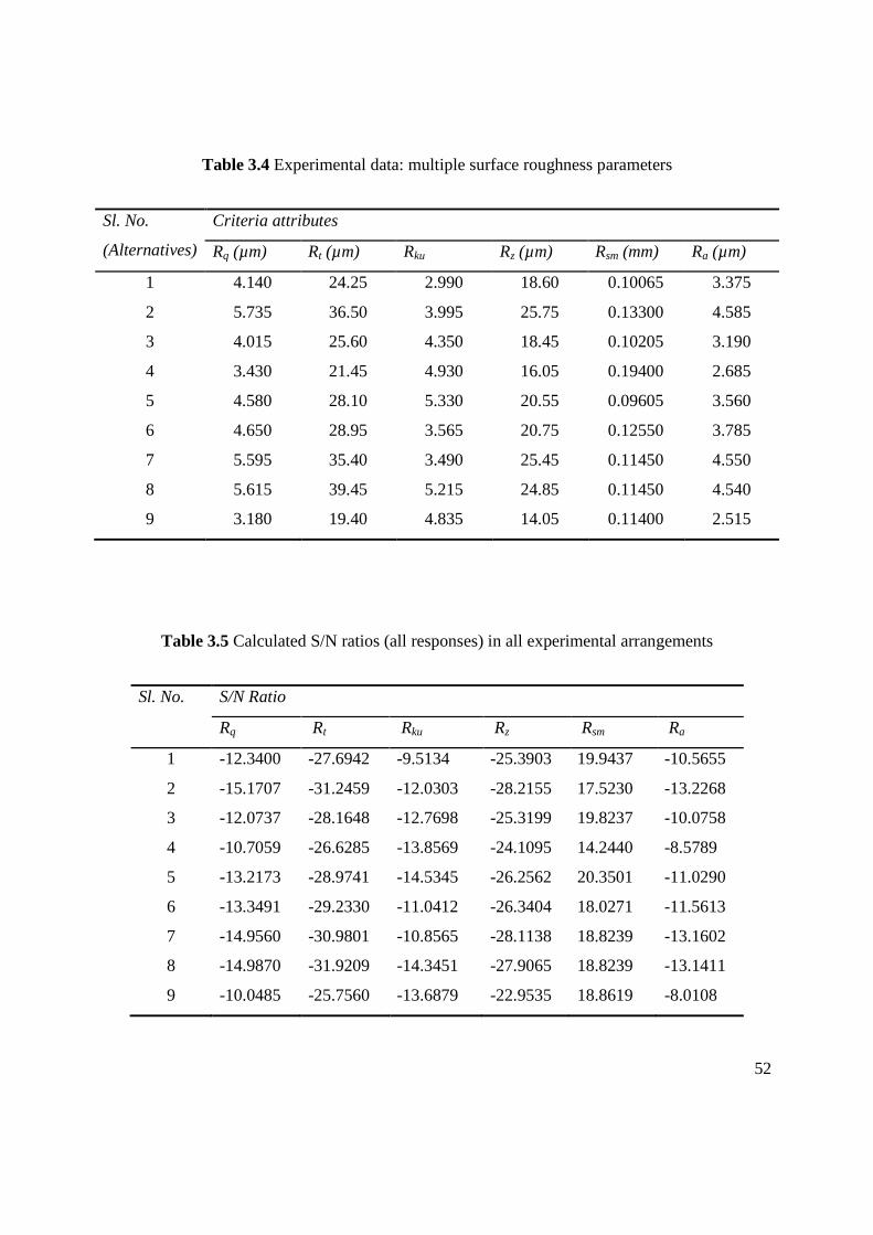
52

Table 3.4 Experimental data: multiple surface roughness parameters

Sl. No.

(Alternatives)

Criteria attributes

Rq (µm) Rt (µm) Rku Rz (µm) Rsm (mm) Ra (µm)

1 4.140 24.25 2.990 18.60 0.10065 3.375

2 5.735 36.50 3.995 25.75 0.13300 4.585

3 4.015 25.60 4.350 18.45 0.10205 3.190

4 3.430 21.45 4.930 16.05 0.19400 2.685

5 4.580 28.10 5.330 20.55 0.09605 3.560

6 4.650 28.95 3.565 20.75 0.12550 3.785

7 5.595 35.40 3.490 25.45 0.11450 4.550

8 5.615 39.45 5.215 24.85 0.11450 4.540

9 3.180 19.40 4.835 14.05 0.11400 2.515

Table 3.5 Calculated S/N ratios (all responses) in all experimental arrangements

Sl. No. S/N Ratio

Rq Rt Rku Rz Rsm Ra

1 -12.3400 -27.6942 -9.5134 -25.3903 19.9437 -10.5655

2 -15.1707 -31.2459 -12.0303 -28.2155 17.5230 -13.2268

3 -12.0737 -28.1648 -12.7698 -25.3199 19.8237 -10.0758

4 -10.7059 -26.6285 -13.8569 -24.1095 14.2440 -8.5789

5 -13.2173 -28.9741 -14.5345 -26.2562 20.3501 -11.0290

6 -13.3491 -29.2330 -11.0412 -26.3404 18.0271 -11.5613

7 -14.9560 -30.9801 -10.8565 -28.1138 18.8239 -13.1602

8 -14.9870 -31.9209 -14.3451 -27.9065 18.8239 -13.1411

9 -10.0485 -25.7560 -13.6879 -22.9535 18.8619 -8.0108

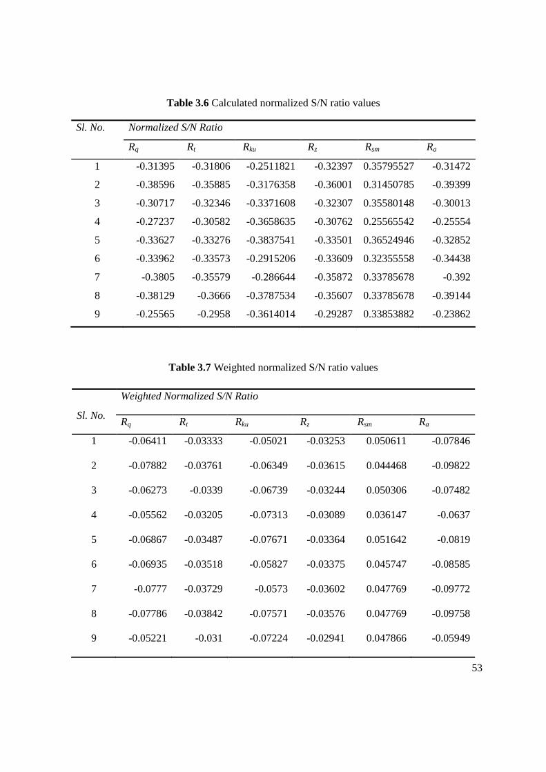
53

Table 3.6 Calculated normalized S/N ratio values

Sl. No. Normalized S/N Ratio

Rq Rt Rku Rz Rsm Ra

1 -0.31395 -0.31806 -0.2511821 -0.32397 0.35795527 -0.31472

2 -0.38596 -0.35885 -0.3176358 -0.36001 0.31450785 -0.39399

3 -0.30717 -0.32346 -0.3371608 -0.32307 0.35580148 -0.30013

4 -0.27237 -0.30582 -0.3658635 -0.30762 0.25565542 -0.25554

5 -0.33627 -0.33276 -0.3837541 -0.33501 0.36524946 -0.32852

6 -0.33962 -0.33573 -0.2915206 -0.33609 0.32355558 -0.34438

7 -0.3805 -0.35579 -0.286644 -0.35872 0.33785678 -0.392

8 -0.38129 -0.3666 -0.3787534 -0.35607 0.33785678 -0.39144

9 -0.25565 -0.2958 -0.3614014 -0.29287 0.33853882 -0.23862

Table 3.7 Weighted normalized S/N ratio values

Sl. No.

Weighted Normalized S/N Ratio

Rq Rt Rku Rz Rsm Ra

1 -0.06411 -0.03333 -0.05021 -0.03253 0.050611 -0.07846

2 -0.07882 -0.03761 -0.06349 -0.03615 0.044468 -0.09822

3 -0.06273 -0.0339 -0.06739 -0.03244 0.050306 -0.07482

4 -0.05562 -0.03205 -0.07313 -0.03089 0.036147 -0.0637

5 -0.06867 -0.03487 -0.07671 -0.03364 0.051642 -0.0819

6 -0.06935 -0.03518 -0.05827 -0.03375 0.045747 -0.08585

7 -0.0777 -0.03729 -0.0573 -0.03602 0.047769 -0.09772

8 -0.07786 -0.03842 -0.07571 -0.03576 0.047769 -0.09758

9 -0.05221 -0.031 -0.07224 -0.02941 0.047866 -0.05949

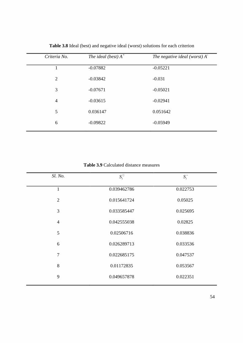
54

Table 3.8 Ideal (best) and negative ideal (worst) solutions for each criterion

Criteria No. The ideal (best) A+ The negative ideal (worst) A-

1 -0.07882 -0.05221

2 -0.03842 -0.031

3 -0.07671 -0.05021

4 -0.03615 -0.02941

5 0.036147 0.051642

6 -0.09822 -0.05949

Table 3.9 Calculated distance measures

Sl. No. +iS −

iS

1 0.039462786 0.022753

2 0.015641724 0.05025

3 0.033585447 0.025695

4 0.042555038 0.02825

5 0.02506716 0.038836

6 0.026289713 0.033536

7 0.022685175 0.047537

8 0.01172835 0.053567

9 0.049657878 0.022351

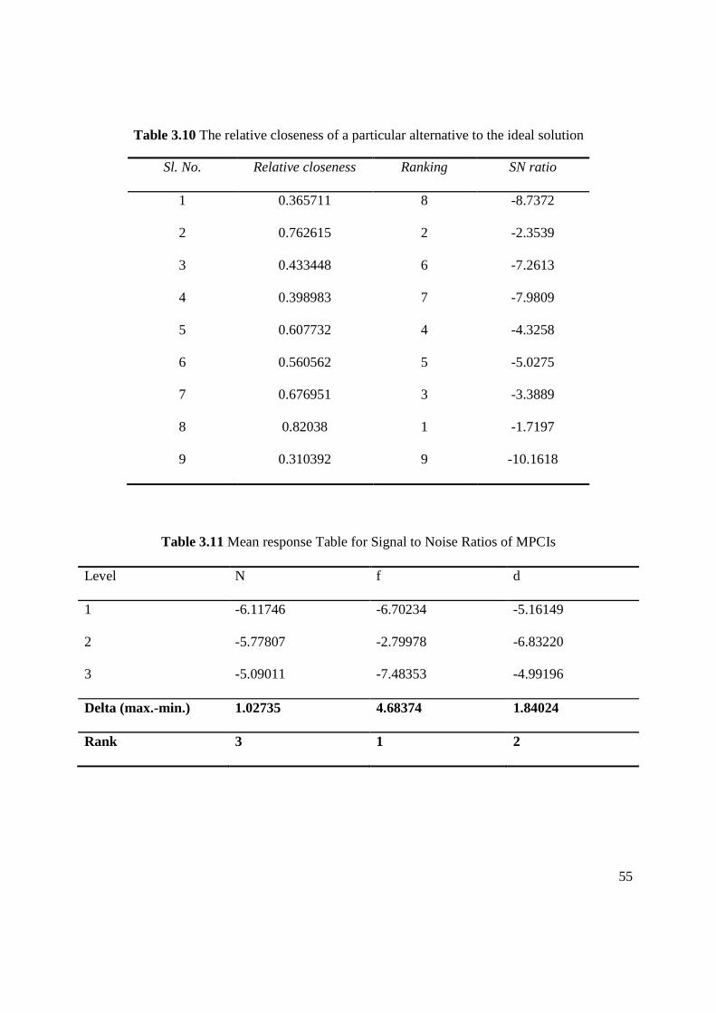
55

Table 3.10 The relative closeness of a particular alternative to the ideal solution

Sl. No. Relative closeness Ranking SN ratio

1 0.365711 8 -8.7372

2 0.762615 2 -2.3539

3 0.433448 6 -7.2613

4 0.398983 7 -7.9809

5 0.607732 4 -4.3258

6 0.560562 5 -5.0275

7 0.676951 3 -3.3889

8 0.82038 1 -1.7197

9 0.310392 9 -10.1618

Table 3.11 Mean response Table for Signal to Noise Ratios of MPCIs Level N f d

1 -6.11746 -6.70234 -5.16149

2 -5.77807 -2.79978 -6.83220

3 -5.09011 -7.48353 -4.99196

Delta (max.-min.) 1.02735 4.68374 1.84024

Rank 3 1 2

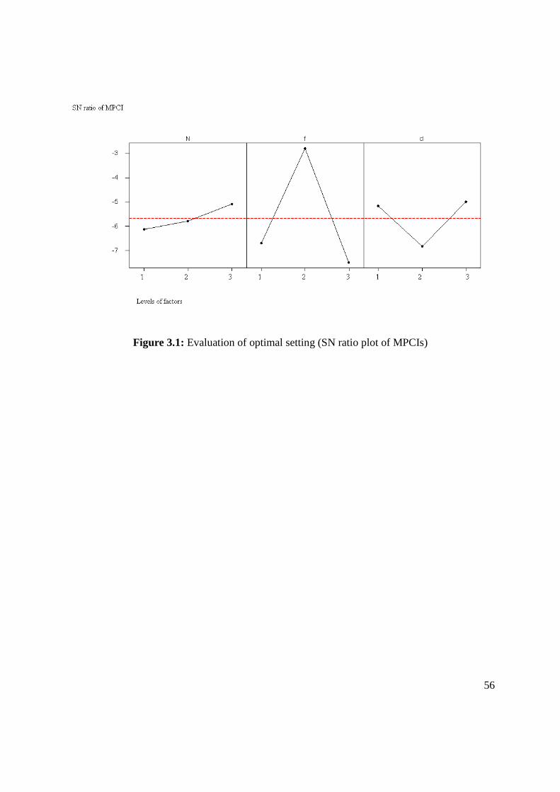
56

Figure 3.1: Evaluation of optimal setting (SN ratio plot of MPCIs)

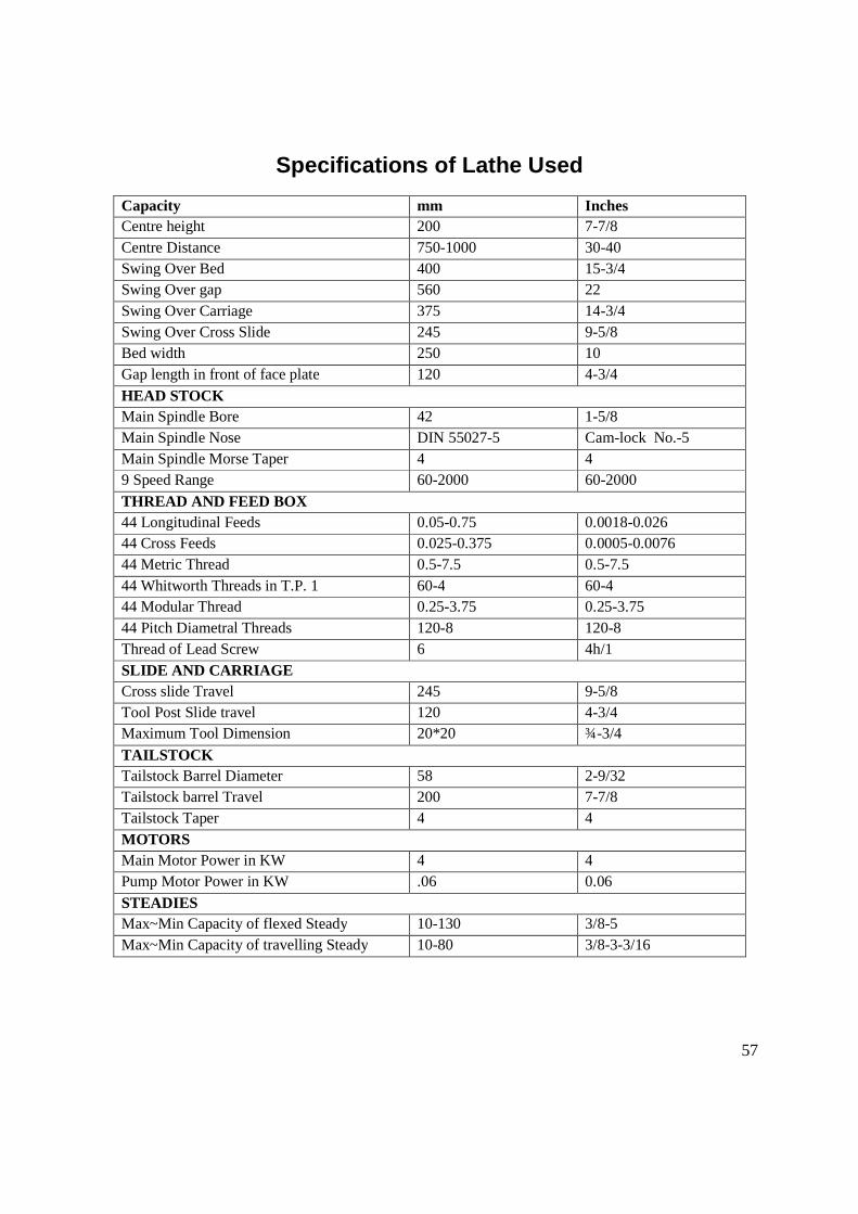
57

Specifications of Lathe Used

Capacity mm Inches Centre height 200 7-7/8 Centre Distance 750-1000 30-40 Swing Over Bed 400 15-3/4 Swing Over gap 560 22 Swing Over Carriage 375 14-3/4 Swing Over Cross Slide 245 9-5/8 Bed width 250 10 Gap length in front of face plate 120 4-3/4

HEAD STOCK Main Spindle Bore 42 1-5/8 Main Spindle Nose DIN 55027-5 Cam-lock No.-5 Main Spindle Morse Taper 4 4 9 Speed Range 60-2000 60-2000

THREAD AND FEED BOX 44 Longitudinal Feeds 0.05-0.75 0.0018-0.026 44 Cross Feeds 0.025-0.375 0.0005-0.0076 44 Metric Thread 0.5-7.5 0.5-7.5 44 Whitworth Threads in T.P. 1 60-4 60-4 44 Modular Thread 0.25-3.75 0.25-3.75 44 Pitch Diametral Threads 120-8 120-8 Thread of Lead Screw 6 4h/1 SLIDE AND CARRIAGE Cross slide Travel 245 9-5/8 Tool Post Slide travel 120 4-3/4 Maximum Tool Dimension 20*20 ¾-3/4

TAILSTOCK Tailstock Barrel Diameter 58 2-9/32 Tailstock barrel Travel 200 7-7/8 Tailstock Taper 4 4 MOTORS Main Motor Power in KW 4 4 Pump Motor Power in KW .06 0.06

STEADIES Max~Min Capacity of flexed Steady 10-130 3/8-5 Max~Min Capacity of travelling Steady 10-80 3/8-3-3/16

58

Chapter 4

Application of Desirability Function, Utility Theory and Fuzzy based Taguchi Method

4.1 Coverage

Glass fiber reinforced polymer (GFRP) is widely used in various engineering application due to

its excellent properties over other engineering materials. The various advantages comprise high

strength to weight ratio, toughness, excellent corrosion and thermal resistance (Adeel et al.,

2010). Hussain et al. (2010) suggested that productivity and quality are the two important

aspects of machining process. Surface roughness and material removal rate greatly influence the

performance of mechanical parts and the production cost. So, quality and productivity is to be

monitored simultaneously at every stage and actions are to be taken in case of deviation from the

target.

Taguchi method is a statistical method developed by Dr. Genichi Taguchi to improve the quality

of manufactured goods. Professional statisticians have welcomed the goals and improvements

brought about by Taguchi methods, particularly by Taguchi's development of designs for

studying variation in the output from targeted value. However, the method is criticized due to

inability to solve multi-objective optimization proposals.

In order to overcome this, utility theory, grey relation theory desirability function approaches

have been reported and well documented in literature. These are widely being applied in

combination with Taguchi method. The disadvantages of aforesaid techniques arise from (i)

improper response weight assignment and (ii) unaccounted response correlation as described in

Chapter 1. Assignment of response priority weight depends on the discretion of decision maker

which may result variation in the optimal results. Moreover, it is assumed that responses are

59

uncorrelated. Interdependence of the responses has been assumed negligible which creates

imprecision, uncertainty as well as vagueness in the final solution. To avoid those limitations,

desirability function (DF) as well as utility theory (UT) based on fuzzy inference system

(FIS) has been proposed in the present chapter. Desirability based fuzzy approach has been

reported by Singh et al. (2011) to optimize bead geometry parameters in submerged arc welding

(SAW) which has been used for meaningful logical aggregation of multiple responses into a

single Multi-Performance-Characteristic Index (MPCI). MPCI has been optimized finally by

Taguchi method.

4.2 Experimentation

The experimental layout (domain of process parameters and orthogonal array design of

experiment) has been selected similar to that described in Chapter 3 (Tables 3.2-3.3). The

experimental set up, cutting tool and measuring instruments that have been used here are similar

as described in Chapter 3. GFRP polyester composite has been selected as specimen whose

compositions have already been furnished in Chapter 3 (Table 3.1). The response features

selected in this experimentation were material removal rate (MRR) and roughness average (Ra)

of the machined composite product. Experimental data have been shown in Table 4.1.

4.3 Application of DF-Fuzzy based Taguchi Method

Block diagram of the proposed methodology has been furnished in Appendix 4. Experimental

data related to turning of GFRP polyester composite corresponding to L9 orthogonal array (OA)

design of experiment (Table 3.3 of Chapter 3) have been explored to calculate desirability

values of individual quality attributes: MRR and Ra(avg). For the surface roughness parameter; a

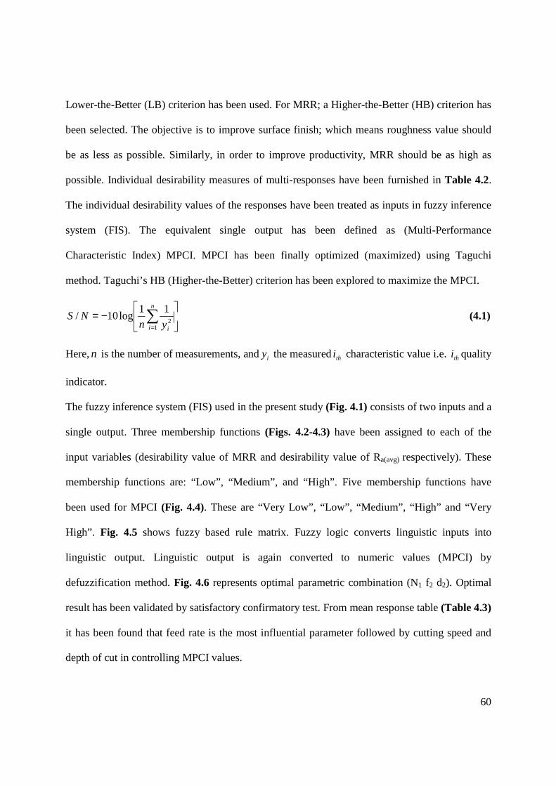
60

Lower-the-Better (LB) criterion has been used. For MRR; a Higher-the-Better (HB) criterion has

been selected. The objective is to improve surface finish; which means roughness value should

be as less as possible. Similarly, in order to improve productivity, MRR should be as high as

possible. Individual desirability measures of multi-responses have been furnished in Table 4.2.

The individual desirability values of the responses have been treated as inputs in fuzzy inference

system (FIS). The equivalent single output has been defined as (Multi-Performance

Characteristic Index) MPCI. MPCI has been finally optimized (maximized) using Taguchi

method. Taguchi’s HB (Higher-the-Better) criterion has been explored to maximize the MPCI.

−= ∑

=

n

i iynNS

12

11log10/ (4.1)

Here,n is the number of measurements, andiy the measuredthi characteristic value i.e. thi quality

indicator.

The fuzzy inference system (FIS) used in the present study (Fig. 4.1) consists of two inputs and a

single output. Three membership functions (Figs. 4.2-4.3) have been assigned to each of the

input variables (desirability value of MRR and desirability value of Ra(avg) respectively). These

membership functions are: “Low”, “Medium”, and “High”. Five membership functions have

been used for MPCI (Fig. 4.4). These are “Very Low”, “Low”, “Medium”, “High” and “Very

High”. Fig. 4.5 shows fuzzy based rule matrix. Fuzzy logic converts linguistic inputs into

linguistic output. Linguistic output is again converted to numeric values (MPCI) by

defuzzification method. Fig. 4.6 represents optimal parametric combination (N1 f2 d2). Optimal

result has been validated by satisfactory confirmatory test. From mean response table (Table 4.3)

it has been found that feed rate is the most influential parameter followed by cutting speed and

depth of cut in controlling MPCI values.

61

4.4 Application of UT-Fuzzy based Taguchi Method

Block diagram of the proposed methodology has been furnished in Appendix 5. Experimental

data related to turning of GFRP polyester composite corresponding to L9 orthogonal array (OA)

design of experiment (Table 4.4) have been investigated to calculate utility values of individual

quality attributes: MRR and Ra(avg). For the surface roughness parameter, a Lower-the-Better

(LB) criterion has been used. For MRR, a Higher-the-Better (HB) criterion has been used. The

justification of individual response selection criteria have already been discussed in Section 4.3

of this chapter. It is felt that a compatible balance should be there for quality (surface quality in

the present case) as well as productivity. Individual utility measures of multi-responses have

been furnished in Table 4.5. The common task is to convert initially these multi-objectives into

an equivalent single objective function. The individual utility values of the responses have been

treated as inputs in fuzzy inference system (FIS). The equivalent single output has been defined

as MPCI. MPCI has been finally optimized (maximized) using Taguchi method. Taguchi’s HB

(Higher-the-Better) criterion has been explored to maximize the MPCI.

FIS (shown in Fig. 4.7) used in the present study consists of two inputs and a single output.

Three membership functions (Figure 4.8-4.9) have been assigned to each of the input variables

(utility value of MRR and utility value of Ravg respectively). These membership functions are:

“Low”, “Medium”, and “High”. For the output (MPCI), five membership functions have been

used: “Very Low”, “Low”, “Medium”, “High” and “Very High” (Fig. 4.10).

Fig. 4.11 shows fuzzy based rule matrix. Fuzzy logic converts linguistic inputs into linguistic

output. Linguistic output is again converted to numeric values (MPCI) by defuzzification

method. Fig. 4.12 represents optimal parametric combination (N2 f3 d2). Optimal result has been

validated by satisfactory confirmatory test. It has been found that predicted signal to noise ratio

62

at optimal setting is 18.5255 (maximum from all entries in Table 4.5).Because S/N ratio is

always to be maximized which means minimum quality loss (in the present case). From mean

response table (Table 4.6) it has been found that feed rate is the most influential parameter

followed by cutting speed and depth of cut in controlling MPCI values.

4.5 Concluding Remarks

In this study desirability function and utility theory based fuzzy models have been developed

consisting of two input variables (material removal rate and roughness average) and one output

variable i.e. MPCI. Through this way a multi-response optimization problem has been converted

to an equivalent single objective optimization problem which has been further solved by Taguchi

philosophy. Accuracy in prediction of the model analysis can be subsequently increased by

increasing number of membership function in the fuzzy system. The proposed procedure has

been simple, effective in developing a robust, versatile and flexible experiment process. In

adapting FIS models it is not necessary to assign response priority weights.

In the contrary, in traditional desirability function based Taguchi approach, it has been viewed

that desirability values of individual responses ( )id are generally aggregated (Eq. 4.2) to

compute an overall desirability( )D . Optimal process environment is then selected through

maximizing overall desirability using Taguchi method.

( )∑

=w

nwn

ww dddD

1

21 .... 21 (4.2)

Here iw is the priority weight ofthi response.

Similarly, in traditional utility concept based Taguchi approach, utility values (preference

numbers) of individual responses( )iU are accumulated (Eq. 4.3) to compute an overall utility

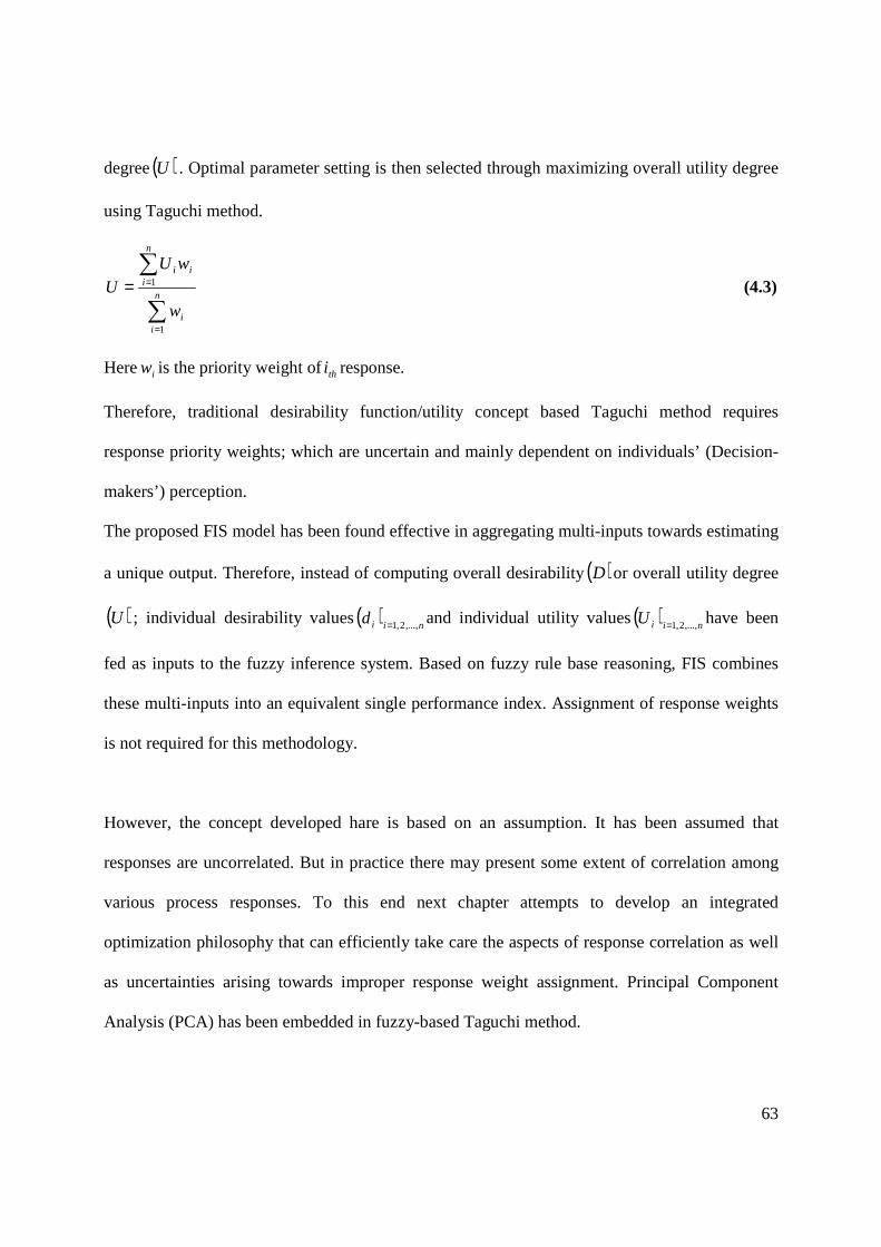
63

degree( )U . Optimal parameter setting is then selected through maximizing overall utility degree

using Taguchi method.

∑

∑

=

==n

ii

n

iii

w

wUU

1

1 (4.3)

Here iw is the priority weight ofthi response.

Therefore, traditional desirability function/utility concept based Taguchi method requires

response priority weights; which are uncertain and mainly dependent on individuals’ (Decision-

makers’) perception.

The proposed FIS model has been found effective in aggregating multi-inputs towards estimating

a unique output. Therefore, instead of computing overall desirability( )D or overall utility degree

( )U ; individual desirability values( ) niid ,...,2,1= and individual utility values( ) niiU ,...,2,1= have been

fed as inputs to the fuzzy inference system. Based on fuzzy rule base reasoning, FIS combines

these multi-inputs into an equivalent single performance index. Assignment of response weights

is not required for this methodology.

However, the concept developed hare is based on an assumption. It has been assumed that

responses are uncorrelated. But in practice there may present some extent of correlation among

various process responses. To this end next chapter attempts to develop an integrated

optimization philosophy that can efficiently take care the aspects of response correlation as well

as uncertainties arising towards improper response weight assignment. Principal Component

Analysis (PCA) has been embedded in fuzzy-based Taguchi method.

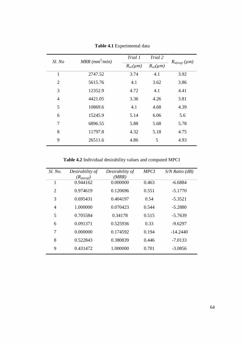
64

Table 4.1 Experimental data

Sl. No MRR (mm3/min) Trial 1 Trial 2

Ra(avg) (µm) Ra1(µm) Ra2(µm)

1 2747.52 3.74 4.1 3.92

2 5615.76 4.1 3.62 3.86

3 12352.9 4.72 4.1 4.41

4 4421.05 3.36 4.26 3.81

5 10869.6 4.1 4.68 4.39

6 15245.9 5.14 6.06 5.6

7 6896.55 5.88 5.68 5.78

8 11797.8 4.32 5.18 4.75

9 26511.6 4.86 5 4.93

Table 4.2 Individual desirability values and computed MPCI

Sl. No. Desirability of (Ra(avg))

Desirability of (MRR)

MPCI S/N Ratio (dB)

1 0.944162 0.000000 0.463 -6.6884

2 0.974619 0.120696 0.551 -5.1770

3 0.695431 0.404197 0.54 -5.3521

4 1.000000 0.070423 0.544 -5.2880

5 0.705584 0.34178 0.515 -5.7639

6 0.091371 0.525936 0.33 -9.6297

7 0.000000 0.174592 0.194 -14.2440

8 0.522843 0.380839 0.446 -7.0133

9 0.431472 1.000000 0.701 -3.0856

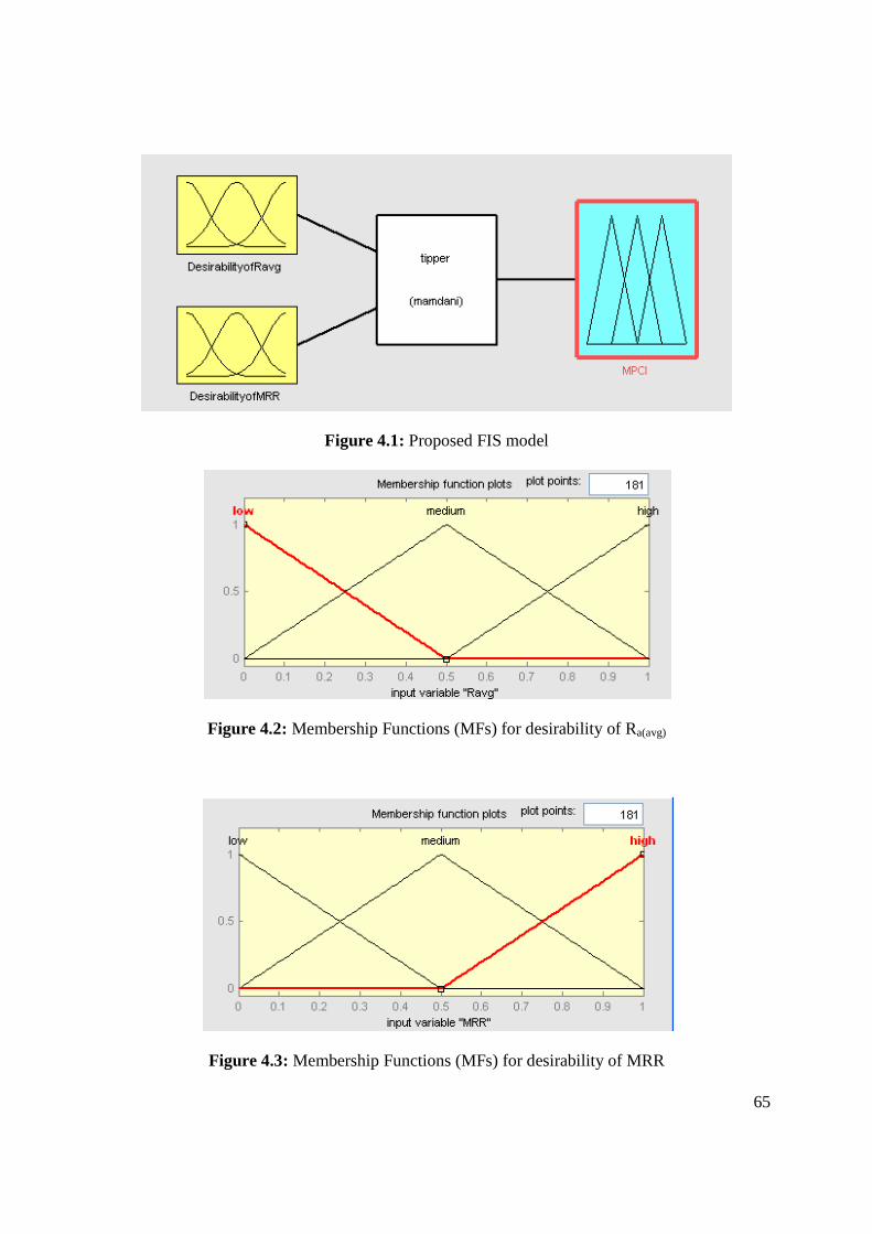
65

Figure 4.1: Proposed FIS model

Figure 4.2: Membership Functions (MFs) for desirability of Ra(avg)

Figure 4.3: Membership Functions (MFs) for desirability of MRR

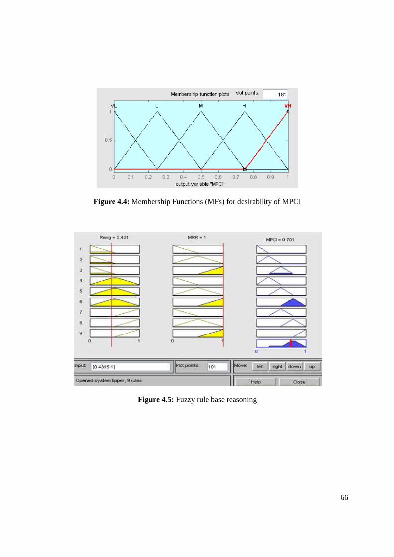
66

Figure 4.4: Membership Functions (MFs) for desirability of MPCI

Figure 4.5: Fuzzy rule base reasoning

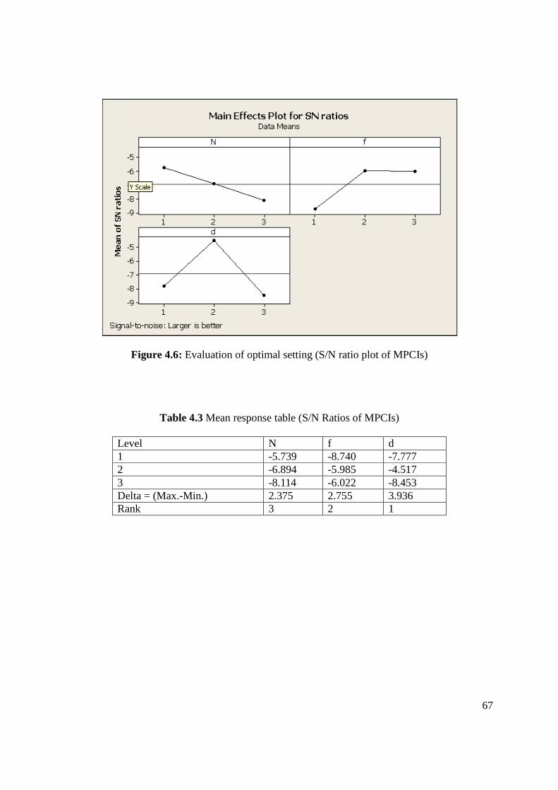
67

Figure 4.6: Evaluation of optimal setting (S/N ratio plot of MPCIs)

Table 4.3 Mean response table (S/N Ratios of MPCIs)

Level N f d 1 -5.739 -8.740 -7.777 2 -6.894 -5.985 -4.517 3 -8.114 -6.022 -8.453 Delta = (Max.-Min.) 2.375 2.755 3.936 Rank 3 2 1

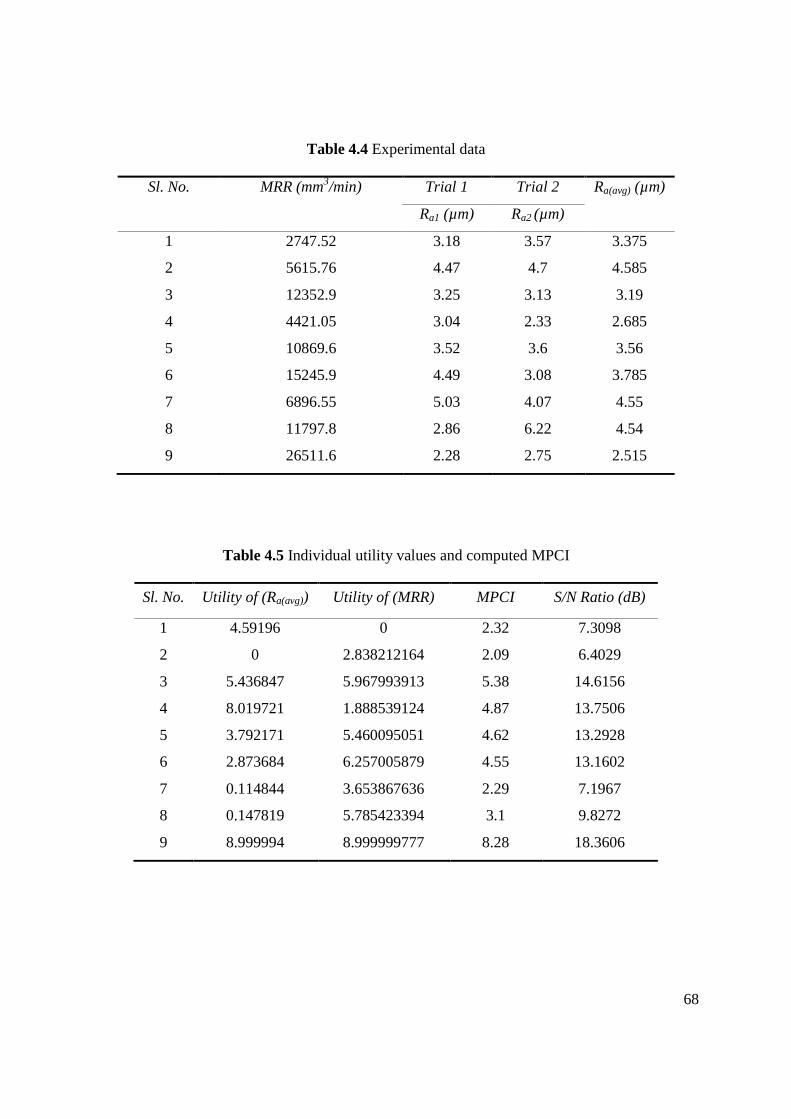
68

Table 4.4 Experimental data

Sl. No. MRR (mm3/min) Trial 1 Trial 2 Ra(avg) (µm)

Ra1 (µm) Ra2 (µm)

1 2747.52 3.18 3.57 3.375

2 5615.76 4.47 4.7 4.585

3 12352.9 3.25 3.13 3.19

4 4421.05 3.04 2.33 2.685

5 10869.6 3.52 3.6 3.56

6 15245.9 4.49 3.08 3.785

7 6896.55 5.03 4.07 4.55

8 11797.8 2.86 6.22 4.54

9 26511.6 2.28 2.75 2.515

Table 4.5 Individual utility values and computed MPCI

Sl. No. Utility of (Ra(avg)) Utility of (MRR) MPCI S/N Ratio (dB)

1 4.59196 0 2.32 7.3098

2 0 2.838212164 2.09 6.4029

3 5.436847 5.967993913 5.38 14.6156

4 8.019721 1.888539124 4.87 13.7506

5 3.792171 5.460095051 4.62 13.2928

6 2.873684 6.257005879 4.55 13.1602

7 0.114844 3.653867636 2.29 7.1967

8 0.147819 5.785423394 3.1 9.8272

9 8.999994 8.999999777 8.28 18.3606

69

Figure 4.7: Proposed FIS model

Figure 4.8: Membership Functions (MFs) for utility of Ra(avg)

Figure 4.9: Membership Functions (MFs) for utility of MRR

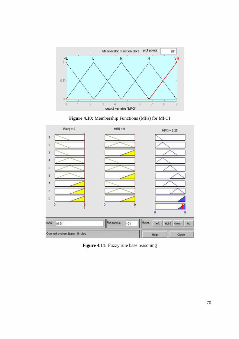
70

Figure 4.10: Membership Functions (MFs) for MPCI

Figure 4.11: Fuzzy rule base reasoning

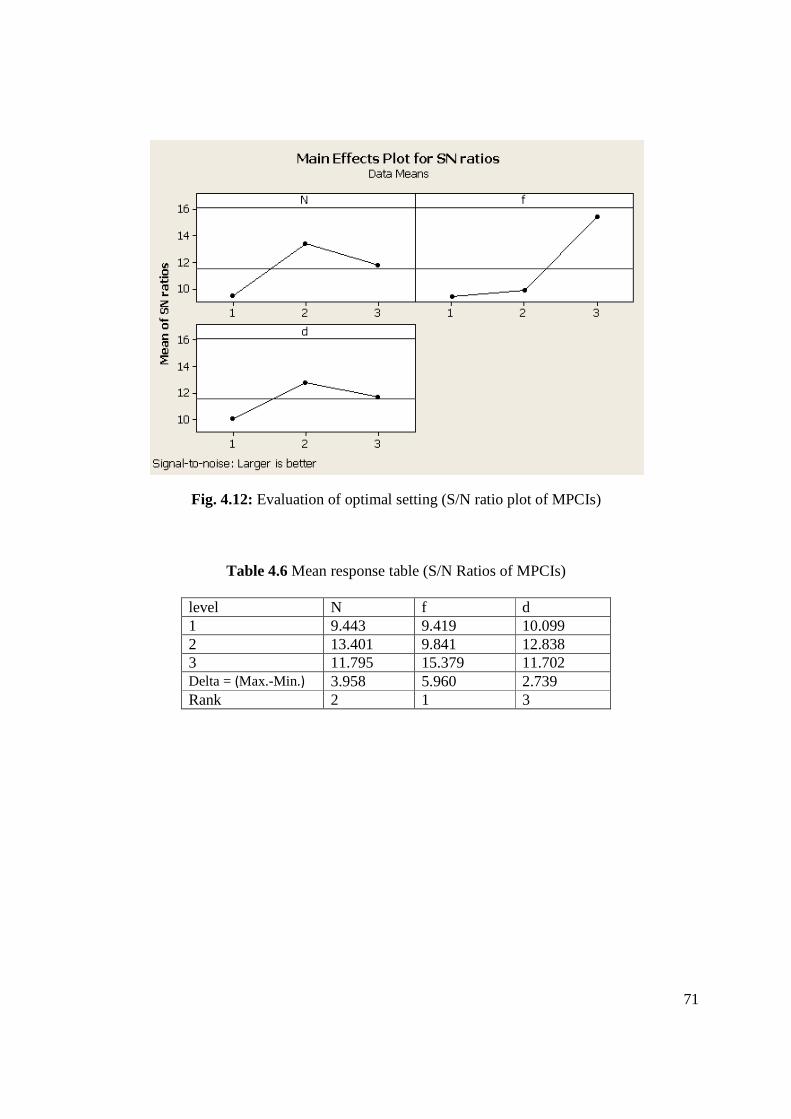
71

Fig. 4.12: Evaluation of optimal setting (S/N ratio plot of MPCIs)

Table 4.6 Mean response table (S/N Ratios of MPCIs)

level N f d 1 9.443 9.419 10.099 2 13.401 9.841 12.838 3 11.795 15.379 11.702 Delta = (Max.-Min.) 3.958 5.960 2.739 Rank 2 1 3

72

Chapter 5 Application of PCA-Fuzzy based Taguchi Method

5.1 Coverage

A PCA-fuzzy expert system integrated with Taguchi method has been proposed here. PCA

has been used to eliminate response correlation and to convert correlated responses into

uncorrelated quality indices. Uncorrelated quality indices are to be fed in Fuzzy Inference

System (FIS) to compute MPCI. Fuzzy logic is an efficient tool immensely applied in the

field of decision engineering (Azadeh et al., 2010; Kumar et al., 2011). The single output of

FIS (i.e. MPCI) has been optimized by Taguchi method.

5.2 Experimentation

The present study has aimed to optimize multiple surface roughness characteristics and MRR

of turned glass fiber reinforced polyester composites. An appropriate process environment

(parameter setting) has been evaluated to minimize various measures (indices) of product

surface roughness characteristics as well as to maximize MRR. Optimal process condition

has been determined from the analysis of experimental data.

The present study has been done through the following plan of experiments.

A. Checking and preparing the centre lathe ready for performing the machining

operation.

B. Cutting GFRP bars and performing initial turning operation in lathe to get desired

dimension ( 15050×φ ) of the work pieces.

C. Calculating weight of each specimen by the high precision digital balance meter

before machining.

73

D. Performing straight turning operation on specimens in various cutting environments

involving various combinations of process control parameters like spindle speed, feed

and depth of cut.

E. Calculating weight of each machined GFRP bars again by the digital balance meter.

F. Calculating MRR of each experiment.

G. Measuring surface roughness with the help of a portable stylus-type profilometer,

Talysurf (Taylor Hobson, Surtronic 3+, UK).

Glass fiber reinforced polyester composite has been selected as work piece material. The

specifications of the work piece material are same as shown in Chapter 3 Table 3.1. The

ISO specification of the tool holder used for the turning operation is a WIDAX tool holder

PC LNR 2020 K12 and the tool insert used for the study are carbide K-20, (CNMA 120408).

In the present study, spindle speed (N, rpm), feed rate (f, mm/min) and depth of cut (d, mm),

have been selected as design factors while other parameters have been assumed to be constant

over the experimental domain. The process variables (design factors) with their values at

different levels have been same as considered in Chapter 3 Table 3.2. It is known that the

selection of the values of the variables is limited by the capacity of the machine used in the

experimentation as well as the recommended specifications for different work piece and tool

material combinations. Therefore, three levels have been selected for each of the aforesaid

three factors. In the present investigation, Taguchi’s L9 orthogonal array (OA) design

(without factorial interaction) has been considered for experimentation (shown in Chapter 3

Table 3.3). The machine used for turning is PINACHO lathe (specifications given at the end

of Chapter 3). The surface roughness parameters have been measured using the stylus-type

profilometer, Talysurf (Taylor Hobson, Surtronic 3+). The values of measured roughness

parameters: (average of two trials) Rq, Ra, Rt, Rku, Rz, Rsm along with material removal rate

(MRR) have been shown in Table 5.1.

74

5.3 Application of PCA-Fuzzy Based Taguchi Approach

Procedural hierarchy of the proposed PCA-fuzzy based Taguchi approach has been furnished

in Appendix 6. Experimental data (corresponding to Table 5.1) have been converted into

corresponding S/N ratios using Eqs. 5.1-5.2. In order to analyze all surface roughness

parameters, a Lower-the-Better (LB) criterion and for MRR, a Higher-the-Better (HB)

criterion has been selected.

)(1

log10/1

2 BettertheLoweryn

NSn

ii −−

−= ∑=

(5.1)

)(11

log10/1

2BettertheHigher

ynNS

n

i i

−−

−= ∑

= (5.2)

Here,n is the number of measurements, andiy the measuredthi characteristic value i.e. thi

quality indicator.

Computed S/N ratios have been furnished in Table 5.2. These S/N ratios have then been

normalized based on Higher-the-Better (HB) criteria using the following equation.

For Higher -the-Better (HB) criterion, the normalized data can be expressed as:

)(min)(max

)(min)()(

kyky

kykykx

ii

iii −

−= (5.3)

Here,

( )kxi is the value of the response k for the thi experiment, ( )kyimin is the smallest value of

( )kyi for the thk response, and ( )kyimax is the largest value of ( )kyi for the thk response.

Normalized S/N ratios have been furnished in Table 5.3. Pearson’s correlation coefficient has

been evaluated next and tabulated in Table 5.4. In all cases nonzero values of correlation

coefficients depict that responses (S/N ratios of all output features) are mutually correlated. In

order to avoid response correlation, PCA has been applied to convert correlated responses

into uncorrelated quality indices called principal components (PCs). Table 5.5 represents

75

principal component analysis i.e. Eigen analysis of the correlation Matrix. After finding

Eigen values, Eigen vectors and correlation coefficients; factor analysis has been carried out

to summarize the data structure in a few dimensions of the data and also to explain the

dimensions associated with large data variability. An orthogonal rotation simply rotates the

axes to give a different perspective. The different methods available are EQUIMAX,

VARIMAX, QUARTIMAX, and ORTHOMAX. A parameter, gamma is determined during

the rotation method. If the method with a low value of gamma is used, the rotation will tend

to simplify the rows of the loadings and if the method with a high value of gamma is used the

rotation will tend to simplify the columns of the loadings. VARIMAX rotation has been used

in the present case because it maximizes the variance of the squared loadings. Rotated factor

loadings and communalities in VARIMAX rotation has been shown in Table 5.6. Fig. 5.1

reveals scree plot obtained in PCA analysis on normalized responses. It has been observed

that first four principal components (PCs) can satisfactorily explain 99.8% data variation.

Therefore, only these PCs have been considered for further analysis. Remaining PCs have

been ignored.

Individual principal components (PC1 to PC4) thus computed have been given in Table 5.7.

PCs have been normalized by using Higher-the-Better (HB) criteria (Eq. 5.2) and

corresponding normalized values have been shown in Table 5.8. Normalized PCs have been

fed as inputs in Fuzzy Inference System (FIS) (Fig. 5.2). The output of the fuzzy inference

system has been defined as MPCI (Table 5.8). This Multi-Performance Characteristic Index

(MPCI) has been finally optimized by using Taguchi methodology. Higher- the- Better (HB)

criterion has been used for optimizing (maximizing) the MPCI (Eq. 5.2).

In calculating MPCI in FIS system, various membership functions (MFs) (Figs. 5.3-5.6) have

been assigned to the seven input variables: The selected membership functions for input

variables are given below.

76

PC1: “Low” and “Medium”.

PC2: “Low”, “Medium” and “High”

PC3: “Very Low”, “Low”, “Medium”, “High” and “Very High”.

PC4: “Low”, “Medium, “High”.

Five membership functions have been selected for MPCI: “Very Low”, “Low”, “Medium”,

“High”, and “Very High” (Fig. 5.7). 15 fuzzy rules (Table 5.9) have been explored for fuzzy

reasoning (Figure 5.8). Fuzzy based rule matrix has been constructed and shown in Table

5.9 (Sivarao et al., 2009; Ali and Zhang, 1999; Gupta et al., 2011). Fuzzy logic converts

linguistic inputs into linguistic output. Linguistic output is again converted to numeric values

(MPCI) by defuzzification method. Numeric values of MPCIs have been tabulated in Table

5.8 with corresponding S/N ratio. S/N ratios of MPCIs have been calculated using Higher-

the-Better (HB) criterion. Fig. 5.9 represents optimal parametric combination (N3 f3 d1).

Optimal result has been validated by satisfactory confirmatory test. Predicted value of S/N

ratio of MPCI becomes -1.26465 and predicted mean is 0.831 (highest among all entries in

Table 5.8). In confirmatory experiment the value came -1.1367. So, quality has improved

using the said optimal setting. Table 5.10 represents mean values table of MPCIs. The degree

of influence of various factors on MPCI can be estimated from this table. It shows that feed

rate is the most significant factor on influencing MPCIs following with spindle speed and

depth of cut.

The aforesaid approach seemed to be effective as it simultaneously optimizes product quality

(multiple surface roughness estimates, in the present case) as well as productivity (MRR).

The outcome of this study bears significant managerial implications. The predicted optimal

setting can satisfactorily be used in mass production line as it maintains twofold requirements

of quality and productivity. It reduces cost for trial and error experimentation, does not solely

77

rely on operators past experience, personal skill; and saves considerable time and production

cost.

5.4 Concluding Remarks

In this study, PCA and fuzzy rule based model has been developed using four input variables

with single output i.e. MPCI. By this way a multi-response optimization problem has been

converted into an equivalent single objective optimization problem which has been further

solved by Taguchi philosophy. The proposed procedure is simple, effective in developing a

robust, versatile and flexible mass production process. Response correlation is eliminated by

PCA analysis. PCs can be aggregated further to compute an overall performance index

(MPCI). In the proposed model it is not required to assign individual response weights. FIS

can efficiently take care of this aspect into its internal hierarchy. Degree of influence of

various process control factors can be investigated easily. Accuracy in prediction of the

model analysis can be subsequently increased by assigning adequate fuzzy rules as well as by

increasing number of membership functions in the fuzzy inference system. This approach

can be recommended for continuous quality improvement and off-line quality control of a

process/product in any manufacturing/ production environment.

The study bears a significant impact on industrial application of the process for manufacture

of composite products in an economic manner. Process optimization can evaluate an

appropriate process environment capable of producing desired quality product. It reduces

time and cost for trial and error experimentation and the obtained best process environment

can be used for mass production line. Work can be extended to study the mechanics of chip

formation, behavior of cutting forces and related aspects at that particular process

environment. The developed optimization methodology may be used to other production

processes as well.

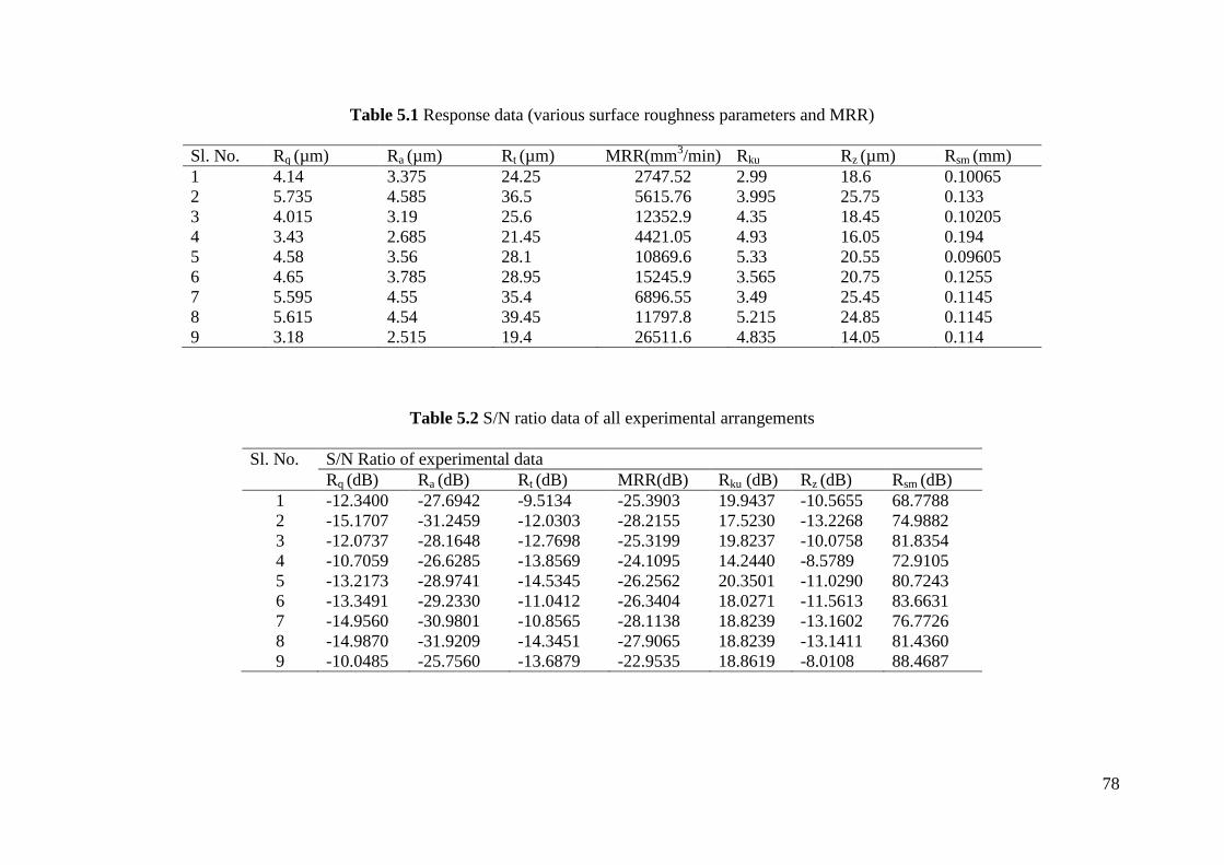
78

Table 5.1 Response data (various surface roughness parameters and MRR)

Sl. No. Rq (µm) Ra (µm) Rt (µm) MRR(mm3/min) Rku Rz (µm) Rsm (mm) 1 4.14 3.375 24.25 2747.52 2.99 18.6 0.10065 2 5.735 4.585 36.5 5615.76 3.995 25.75 0.133 3 4.015 3.19 25.6 12352.9 4.35 18.45 0.10205 4 3.43 2.685 21.45 4421.05 4.93 16.05 0.194 5 4.58 3.56 28.1 10869.6 5.33 20.55 0.09605 6 4.65 3.785 28.95 15245.9 3.565 20.75 0.1255 7 5.595 4.55 35.4 6896.55 3.49 25.45 0.1145 8 5.615 4.54 39.45 11797.8 5.215 24.85 0.1145 9 3.18 2.515 19.4 26511.6 4.835 14.05 0.114

Table 5.2 S/N ratio data of all experimental arrangements

Sl. No. S/N Ratio of experimental data Rq (dB) Ra (dB) Rt (dB) MRR(dB) Rku (dB) Rz (dB) Rsm (dB)

1 -12.3400 -27.6942 -9.5134 -25.3903 19.9437 -10.5655 68.7788 2 -15.1707 -31.2459 -12.0303 -28.2155 17.5230 -13.2268 74.9882 3 -12.0737 -28.1648 -12.7698 -25.3199 19.8237 -10.0758 81.8354 4 -10.7059 -26.6285 -13.8569 -24.1095 14.2440 -8.5789 72.9105 5 -13.2173 -28.9741 -14.5345 -26.2562 20.3501 -11.0290 80.7243 6 -13.3491 -29.2330 -11.0412 -26.3404 18.0271 -11.5613 83.6631 7 -14.9560 -30.9801 -10.8565 -28.1138 18.8239 -13.1602 76.7726 8 -14.9870 -31.9209 -14.3451 -27.9065 18.8239 -13.1411 81.4360 9 -10.0485 -25.7560 -13.6879 -22.9535 18.8619 -8.0108 88.4687

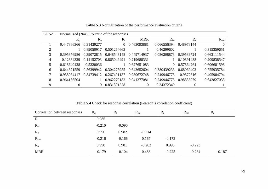
79

Table 5.3 Normalization of the performance evaluation criteria

Sl. No. Normalized (Nor) S/N ratio of the responses Rq Ra Rt MRR Rku Rz Rsm

1 0.447366366 0.31439277 0 0.463093881 0.066556394 0.48978144 0 2 1 0.89050917 0.501264663 1 0.46299602 1 0.315359651 3 0.395376986 0.39072815 0.648543148 0.449714937 0.086208873 0.39589724 0.663111544 4 0.12834329 0.14152703 0.865049491 0.219688331 1 0.10891488 0.209838547 5 0.618640428 0.5220036 1 0.627651083 0 0.57864264 0.606681598 6 0.644371559 0.56399942 0.304275955 0.643652604 0.380439233 0.68069402 0.755935784 7 0.958084417 0.84739412 0.267491187 0.980672748 0.249946775 0.9872316 0.405984794 8 0.964136504 1 0.962279182 0.941277081 0.249946775 0.98356979 0.642827033 9 0 0 0.831391528 0 0.24372349 0 1

Table 5.4 Check for response correlation (Pearson’s correlation coefficient)

Correlation between responses Rq Rt Rku Rz Rsm Ra

Rt 0.985

Rku -0.210 -0.090

Rz 0.996 0.982 -0.214

Rsm -0.216 -0.166 0.167 -0.172

Ra 0.998 0.981 -0.262 0.993 -0.223

MRR -0.179 -0.104 0.483 -0.225 -0.264 -0.187

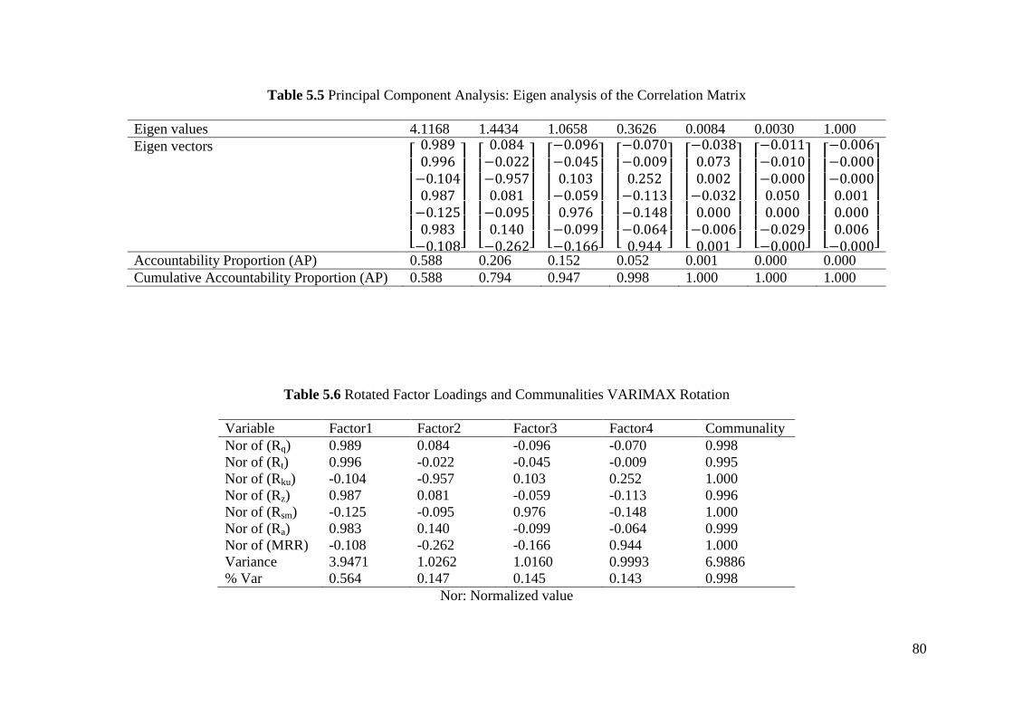
80

Table 5.5 Principal Component Analysis: Eigen analysis of the Correlation Matrix

Eigen values 4.1168 1.4434 1.0658 0.3626 0.0084 0.0030 1.000 Eigen vectors

�������

0.9890.996

0.1040.987

0.1250.983

0.108�������

�������

0.0840.0220.9570.081

0.0950.140

0.262�������

�������0.0960.0450.103

0.0590.976

0.0990.166�

������

�������0.0700.0090.252

0.1130.1480.0640.944 �

������

�������0.0380.0730.002

0.0320.000

0.0060.001 �

������

�������0.0110.0100.0000.0500.000

0.0290.000�

������

�������0.0060.0000.0000.0010.0000.006

0.000�������

Accountability Proportion (AP) 0.588 0.206 0.152 0.052 0.001 0.000 0.000 Cumulative Accountability Proportion (AP) 0.588 0.794 0.947 0.998 1.000 1.000 1.000

Table 5.6 Rotated Factor Loadings and Communalities VARIMAX Rotation

Variable Factor1 Factor2 Factor3 Factor4 Communality Nor of (Rq) 0.989 0.084 -0.096 -0.070 0.998 Nor of (Rt) 0.996 -0.022 -0.045 -0.009 0.995 Nor of (Rku) -0.104 -0.957 0.103 0.252 1.000 Nor of (Rz) 0.987 0.081 -0.059 -0.113 0.996 Nor of (Rsm) -0.125 -0.095 0.976 -0.148 1.000 Nor of (Ra) 0.983 0.140 -0.099 -0.064 0.999 Nor of (MRR) -0.108 -0.262 -0.166 0.944 1.000 Variance 3.9471 1.0262 1.0160 0.9993 6.9886 % Var 0.564 0.147 0.145 0.143 0.998

Nor: Normalized value

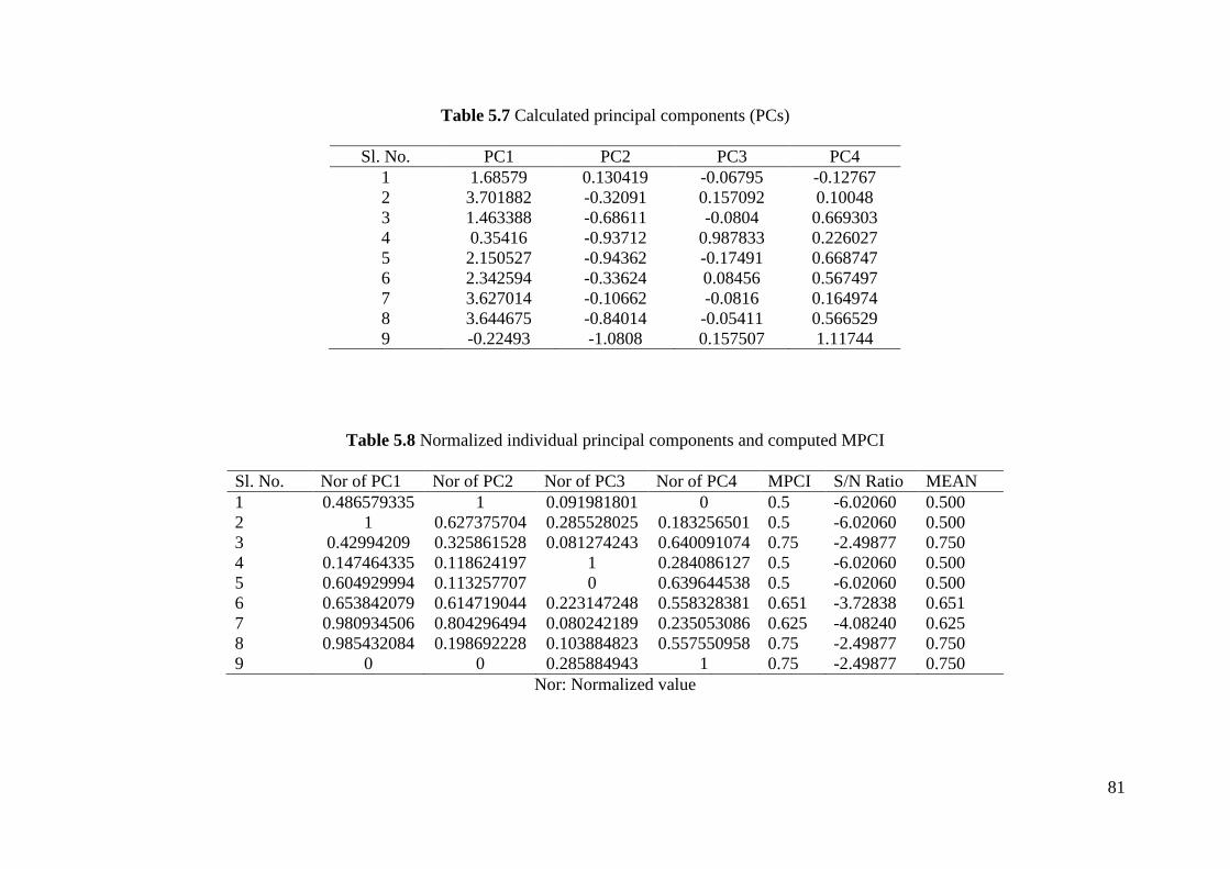
81

Table 5.7 Calculated principal components (PCs)

Sl. No. PC1 PC2 PC3 PC4 1 1.68579 0.130419 -0.06795 -0.12767 2 3.701882 -0.32091 0.157092 0.10048 3 1.463388 -0.68611 -0.0804 0.669303 4 0.35416 -0.93712 0.987833 0.226027 5 2.150527 -0.94362 -0.17491 0.668747 6 2.342594 -0.33624 0.08456 0.567497 7 3.627014 -0.10662 -0.0816 0.164974 8 3.644675 -0.84014 -0.05411 0.566529 9 -0.22493 -1.0808 0.157507 1.11744

Table 5.8 Normalized individual principal components and computed MPCI

Sl. No. Nor of PC1 Nor of PC2 Nor of PC3 Nor of PC4 MPCI S/N Ratio MEAN 1 0.486579335 1 0.091981801 0 0.5 -6.02060 0.500 2 1 0.627375704 0.285528025 0.183256501 0.5 -6.02060 0.500 3 0.42994209 0.325861528 0.081274243 0.640091074 0.75 -2.49877 0.750 4 0.147464335 0.118624197 1 0.284086127 0.5 -6.02060 0.500 5 0.604929994 0.113257707 0 0.639644538 0.5 -6.02060 0.500 6 0.653842079 0.614719044 0.223147248 0.558328381 0.651 -3.72838 0.651 7 0.980934506 0.804296494 0.080242189 0.235053086 0.625 -4.08240 0.625 8 0.985432084 0.198692228 0.103884823 0.557550958 0.75 -2.49877 0.750 9 0 0 0.285884943 1 0.75 -2.49877 0.750

Nor: Normalized value

82

Figure 5.1: Principal component score

Figure 5.2: Proposed FIS model

Figure 5.3: MFs for PC1

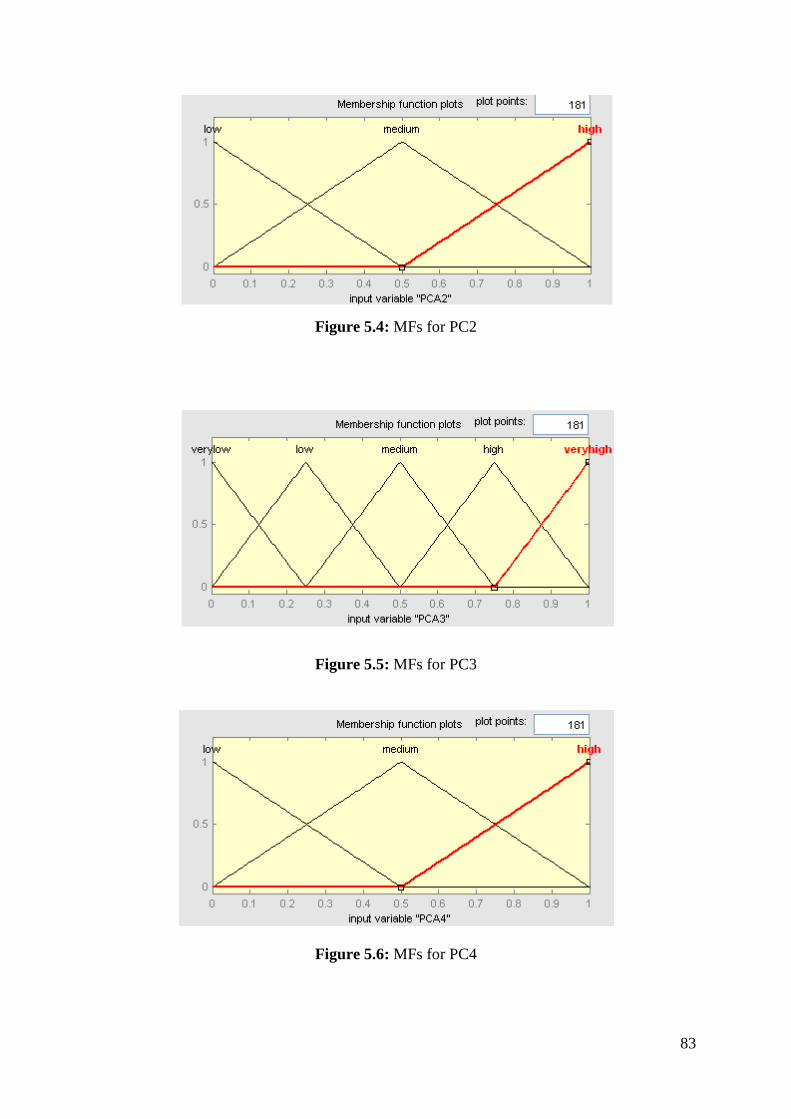
83

Figure 5.4: MFs for PC2

Figure 5.5: MFs for PC3

Figure 5.6: MFs for PC4

84

Figure 5.7: MFs for MPCI

Figure 5.8: Fuzzy rule base reasoning

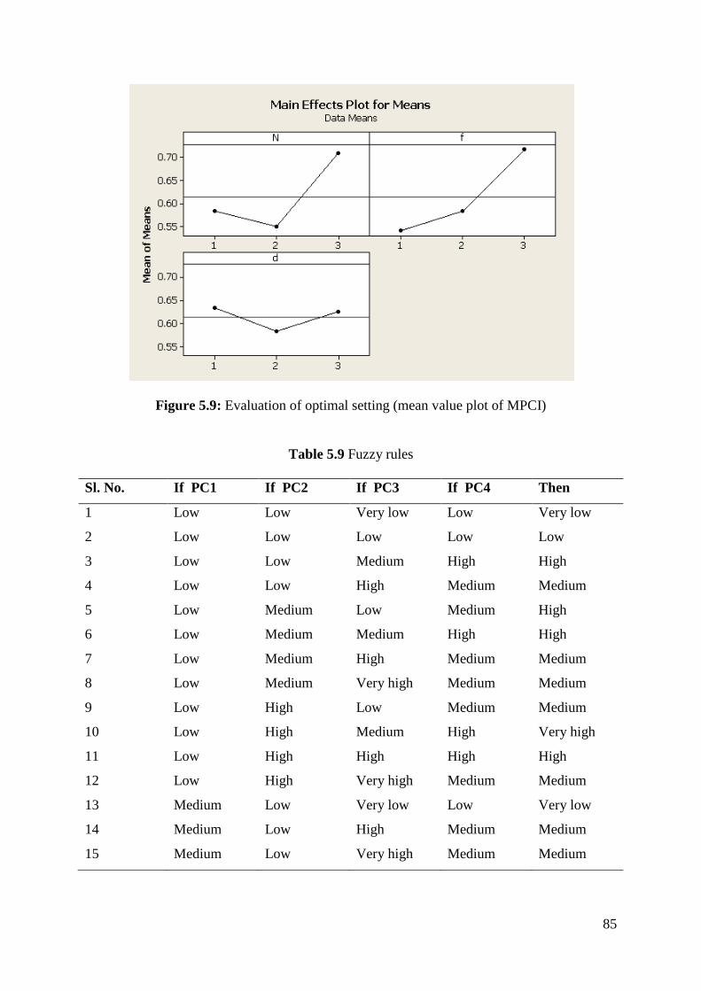
85

Figure 5.9: Evaluation of optimal setting (mean value plot of MPCI)

Table 5.9 Fuzzy rules

Sl. No. If PC1 If PC2 If PC3 If PC4 Then

1 Low Low Very low Low Very low

2 Low Low Low Low Low

3 Low Low Medium High High

4 Low Low High Medium Medium

5 Low Medium Low Medium High

6 Low Medium Medium High High

7 Low Medium High Medium Medium

8 Low Medium Very high Medium Medium

9 Low High Low Medium Medium

10 Low High Medium High Very high

11 Low High High High High

12 Low High Very high Medium Medium

13 Medium Low Very low Low Very low

14 Medium Low High Medium Medium

15 Medium Low Very high Medium Medium

86

Table 5.10 Response table for means (of MPCI)

Level N f d 1 0.5883 0.5417 0.6337 2 0.5503 0.5833 0.5833 3 0.7083 0.7170 0.6250

Delta 0.1580 0.1753 0.0503 Rank 2 1 3

Delta: (Maximum-Minimum)

87

Chapter 6

ANFIS based Prediction Modeling

6.1 Coverage

Glass fiber reinforced epoxy comprises high strength to weight ratio, toughness, excellent

corrosion and thermal resistance over other engineering materials. With increasing applications

of GFRP composites; machining and machinability aspects of composites are very important and

need to be studied in detail. Effect of process parameters on various machining performance,

quality and productivity need to be examined critically.

Surface roughness is an important product quality feature in any machining operation. Attempts

were made by pioneer researchers towards prediction-modeling and optimization of surface

roughness of a variety of product in various machining operations.

Literature seems rich in addressing issues of surface roughness: modeling, prediction and

optimization, mostly in machining conventional metals. Machining aspects of composites have

been addressed in literature to a limited extent. To this end present study highlights a case study

in machining glass fiber reinforced epoxy composite. Predictive model has been developed using

ANFIS to estimate surface roughness for a given set of input parameters. ANFIS utilizes the

concept of neural network and fuzzy logic.

Fuzzy logic is an effective technique for the identification and control of complex non-linear

systems. Fuzzy logic is particularly attractive due to its ability to solve problems in the absence

of accurate mathematical models. The conventional technique to model the surface roughness

results in significant discrepancies between simulation results and experimental data. Artificial

Neural Networks (ANNs) have been widely used for modeling complex manufacturing process

due to their learning and generalization capabilities, accommodation of non-linear variables,

88

adaptively to changing environments and resistance to missing data. Jang (1993) applied ANN

in surface roughness study and correlated surface roughness with cutting vibrations. ANNs have

been widely applied in modeling different metal cutting operations, such as turning, milling and

drilling. The knowledge and the pattern are difficult to learn by the neural network. But fuzzy

logic models are easy to cover because they use linguistic terms in the form of IF-THEN rules. A

neural network with their learning capabilities can be used to learn the fuzzy decision rules, thus

creating a hybrid intelligent system. The fuzzy system provides expert knowledge to be used by

the neural network. A fuzzy inference system consists of three components. First, a rule base

contains a selection of fuzzy rules. Second, a database defines the membership functions used in

the rules and, finally, a reasoning mechanism to carry out the inference procedure on the rules

and given facts. This combines the advantageous characteristics of neural network and fuzzy

system.

Jiao et al. (2004) used fuzzy adaptive network to model surface roughness in turning operation.

A neural fuzzy system was used to predict surface roughness in milling operations (Chen and

Savage, 2001; Lou and Chen, 1999). A compound fuzzy inference neural network was used for

cutting process online monitoring (Lin et al. 2002). Jang (1993) proposed a combination of a

neural network and fuzzy logic, called an adaptive neuro-fuzzy inference system. ANFIS is a

fuzzy inference system implemented in the model of neural networks. A machining process has

been modeled in the present study using ANFIS to predict the effect of machining variables like

speed, feed and depth of cut on material removal rate (MRR) and surface finish of the machined

composite product. The procedural hierarchy for ANFIS modeling towards prediction of MRR

and surface roughness has been shown in Fig. 6.1. The details of ANFIS have already been

discussed in Chapter 2, Section 2.7.

89

6.2 Experimentation

Glass fiber reinforced epoxy composite (fiber orientation 900) (E-glass: R099 1200 P556) has

been selected as work piece material. Above mat consisted of an E-glass with 72.5 GPa modulus

and density of 2590 kg/m3. Straight turning operation has been performed on aforesaid composite

specimens on PINACO lathe. In the present experimental part, spindle speed (N, rpm), feed rate

(f, mm/min) and depth of cut (d, mm), have been selected as design factors while other

parameters have been assumed to be constant over the experimental domain. The process

variables (design factors) with their values at different levels have been listed in Table 6.1. The

ISO specification of the tool holder used for the turning operation is a WIDAX tool holder PC

LNR 2020 K12 and the tool insert used for the study are carbide K-20, (CNMA 120408). A 3-

factor-3-level full factorial design (Table 6.2) has been used in this experiment. Corresponding

to each experimental run, data on MRR and roughness average of the machined work piece have

been collected. The experimental layout and the collected response data are shown in Table 6.2.

Experimental data have been utilized for prediction-modeling of output responses.

Representative snaps of machining of glass fiber reinforced epoxy composite have been given in

Appendix 8.

6.3 Data Analysis and Results

6.3.1 Prediction-Modeling for Surface Roughness

In this part an ANFIS based prediction model has been established for roughness average of

finished composite product for machining of glass fiber reinforced epoxy composites. The whole

experimental data set has been divided into training set, testing set and checking data set. A total

90

of 27 data sets as shown in Table 6.2 have been used. Among 27 data, 21 have been considered

as training data and 6 as testing data. The Fig. 6.2 shows the procedure for developing the

ANFIS model. During training, a five layered ANFIS model has been constructed as discussed.

The number of nodes in the second layer has been increased gradually during training starting

with two. It has been observed that the error has converged (decreasing) by increasing the nodes

up to three. Hence, the number of nodes in second layer has been set fixed to three and further

analysis has been carried out. The five layers have been known as one input, three hidden and

one output layer. Three Gaussian type membership functions (guessmf) has been chosen for

input as shown in Figs. 6.3-6.5 and constant type membership function has been used for output

during generating FIS. After that 6 data have been used for testing to verify the accuracy of the

proposed model. The generated model structure of ANFIS has been shown in Fig. 6.6.

The pattern of variation of actual and predicted data has been shown in Figs. 6.7-6.8. The blue

dots indicate actual output data and red dots represent predicted data. The plots show the

coherence nature of the data distribution. The surface plot has been shown in Fig. 6.9. It can be

observed that the surface covers the total landscape of decision space. A sample set of rule

generation for prediction of surface roughness has been shown in Fig. 6.10. The on-line

predicted surface roughness by ANFIS has an average percent error of 9% when a Gaussian

membership function has been applied. This achieves an accuracy of prediction of 91%. ANFIS

technique in parallel with power spectrum analysis can be used efficiently to predict the surface

roughness on-line during turning process. The objective of improving the surface roughness is to

eliminate the discrepancies thus reduces the defective rate of the finished part and thereby,

increasing product quality.

91

6.3.2 Prediction-Modeling for MRR

In this part an ANFIS based prediction model has been established for material removal rate for

machining of glass fiber reinforced epoxy composites.

The first and the fourth layer are the adaptive layers in ANFIS. The parameters in the first layer

are called premise parameters and consequent parameters in the fourth layer. The least square

method is used to optimize the consequent parameter with the premise parameters fixed. The

Gradient descent method is used to adjust optimally the premise parameter corresponding to the

fuzzy sets in input domain. The output is calculated with the help of consequent parameters.

For anticipating MRR, training database with respect to cutting parameters is necessary to build

in an ANFIS. A total set of 21 has been taken for training in ANFIS from the set of 27 dataset

obtained from the experiment shown in Table 6.3. The training data are responsible for

membership function parameters. The training data does not represent the overall features of the

presented model due to the data taken during the noisy environment. So, it is necessary to

validate the FIS by testing the data set. The testing data is useful in checking the generalization

capability of the Fuzzy inference system. The 6 dataset from the aforesaid 27 dataset has been

taken for testing to verify the accuracy of the predicted values of MRR shown in Table 6.3. In

this model N, f, d has been taken as the inputs and MRR has been considered as the output.

Gaussian membership function has been used for both the input and output variables shown in

Fig. 6.11. The number of fuzzy rules in a fuzzy system is related to the number of fuzzy sets for

each input variables and the 3 inputs are classified into 3 fuzzy sets. Therefore, maximum

number of rules for this model becomes 27 as shown in Fig. 6.12.

The pattern of variation of actual and predicted data has been shown in Figs. 6.13-6.14. The blue

dots indicate actual output and red dots represents predicted data. The plots exhibit the coherence

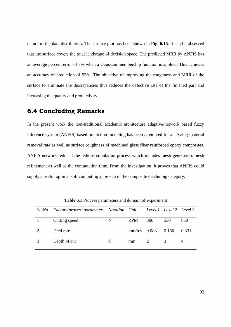
92

nature of the data distribution. The surface plot has been shown in Fig. 6.15. It can be observed

that the surface covers the total landscape of decision space. The predicted MRR by ANFIS has

an average percent error of 7% when a Gaussian membership function is applied. This achieves

an accuracy of prediction of 93%. The objective of improving the roughness and MRR of the

surface to eliminate the discrepancies thus reduces the defective rate of the finished part and

increasing the quality and productivity.

6.4 Concluding Remarks

In the present work the non-traditional academic architecture adaptive-network based fuzzy

inference system (ANFIS) based prediction-modeling has been attempted for analyzing material

removal rate as well as surface roughness of machined glass fiber reinforced epoxy composites.

ANFIS network reduced the tedious simulation process which includes mesh generation, mesh

refinement as well as the computation time. From the investigation, it proves that ANFIS could

supply a useful optimal soft computing approach in the composite machining category.

Table 6.1 Process parameters and domain of experiment

Sl. No. Factors/process parameters Notation Unit Level 1 Level 2 Level 3

1 Cutting speed N RPM 360 530 860

2 Feed rate f mm/rev 0.083 0.166 0.331

3 Depth of cut d mm 2 3 4

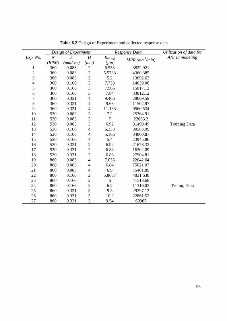
93

Table 6.2 Design of Experiment and collected response data

Exp. No. Design of Experiment Response Data Utilization of data for

ANFIS modeling N (RPM)

F (mm/rev)

D (mm)

Ra(avg)

(µm) MRR (mm3/min)

1 360 0.083 2 6.533 3822.921

Training Data

2 360 0.083 2 5.5733 4360.385 3 360 0.083 2 5.2 13092.62 4 360 0.166 3 7.733 14639.08 5 360 0.166 3 7.966 15817.12 6 360 0.166 3 7.84 33812.12 7 360 0.331 4 9.466 28669.59 8 360 0.331 4 9.63 11502.97 9 360 0.331 4 11.133 9560.534 10 530 0.083 3 7.2 25364.91 11 530 0.083 3 7 22683.2 12 530 0.083 3 6.92 31499.49 13 530 0.166 4 6.333 30503.99 14 530 0.166 4 5.166 34800.87 15 530 0.166 4 5.4 23945.86 16 530 0.331 2 6.92 21678.33 17 530 0.331 2 6.88 16302.09 18 530 0.331 2 6.86 27904.81 19 860 0.083 4 7.033 22042.64 20 860 0.083 4 6.84 75021.07 21 860 0.083 4 6.9 75401.89 22 860 0.166 2 5.8667 4831.638

Testing Data

23 860 0.166 2 6 41518.68 24 860 0.166 2 6.2 11316.03 25 860 0.331 3 9.3 29397.13 26 860 0.331 3 10.2 22861.52 27 860 0.331 3 9.54 69367

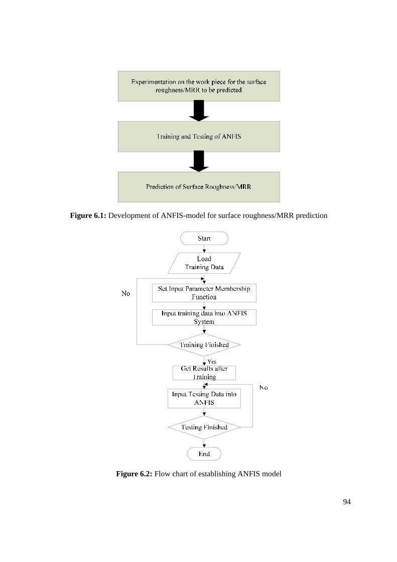
94

Figure 6.1: Development of ANFIS-model for surface roughness/MRR prediction

Figure 6.2: Flow chart of establishing ANFIS model

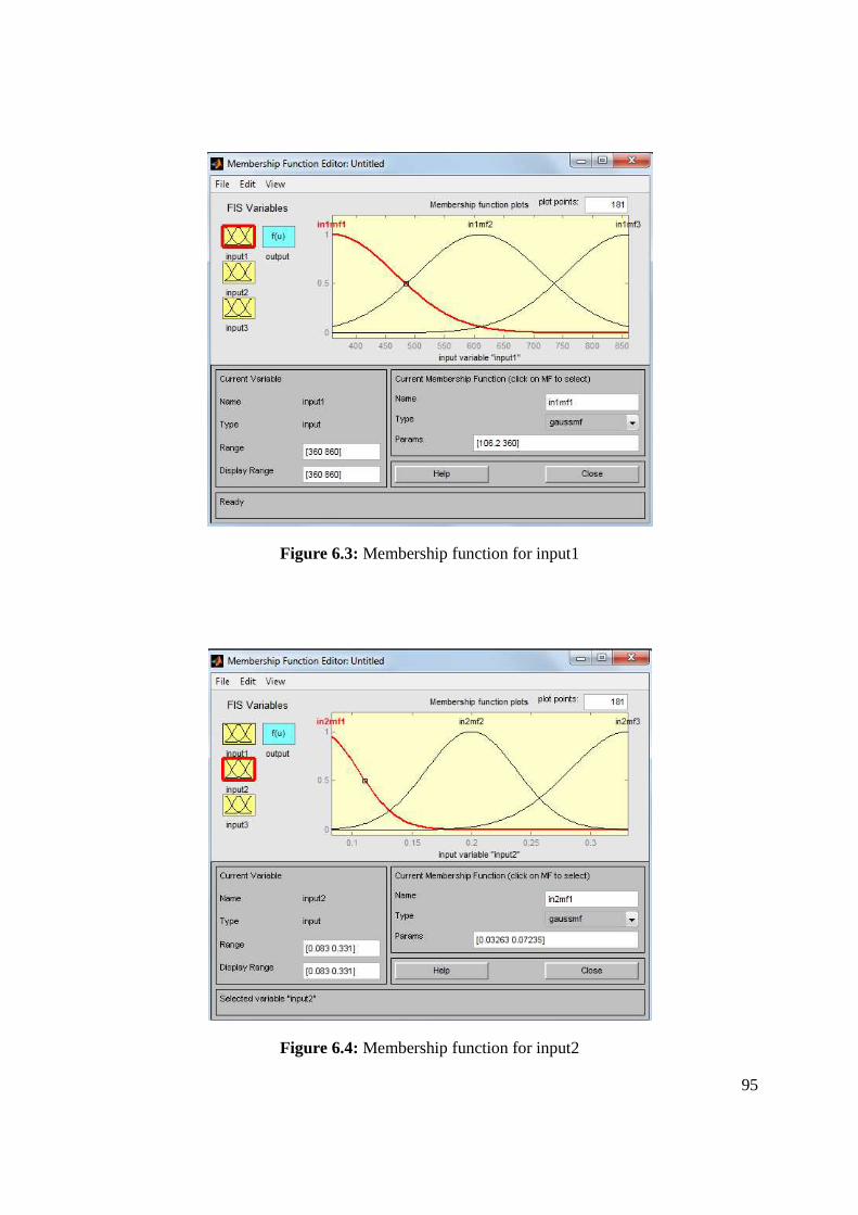
95

Figure 6.3: Membership function for input1

Figure 6.4: Membership function for input2

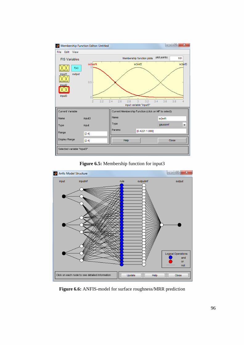
96

Figure 6.5: Membership function for input3

Figure 6.6: ANFIS-model for surface roughness/MRR prediction

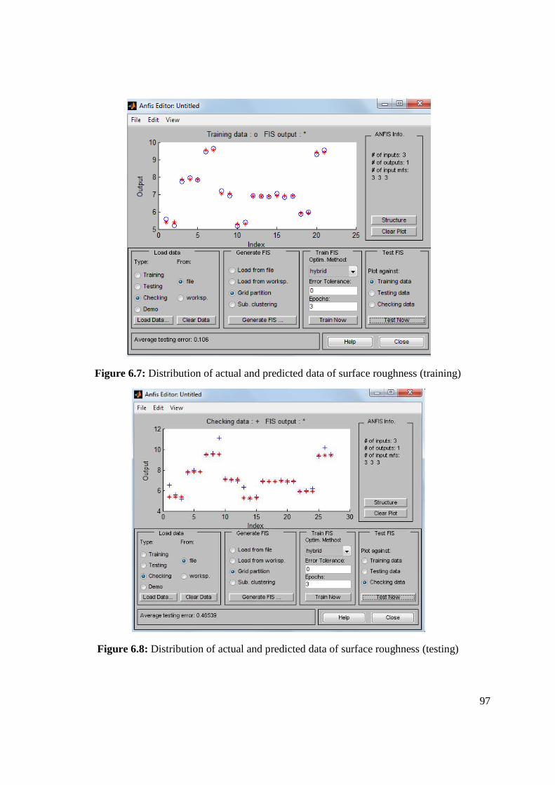
97

Figure 6.7: Distribution of actual and predicted data of surface roughness (training)

Figure 6.8: Distribution of actual and predicted data of surface roughness (testing)

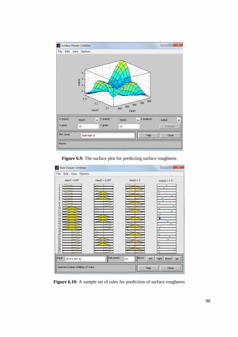
98

Figure 6.9: The surface plot for predicting surface roughness

Figure 6.10: A sample set of rules for prediction of surface roughness

99

Figure 6.11: Membership function for input(s) and output

Figure 6.12: A sample set of rules for prediction of MRR

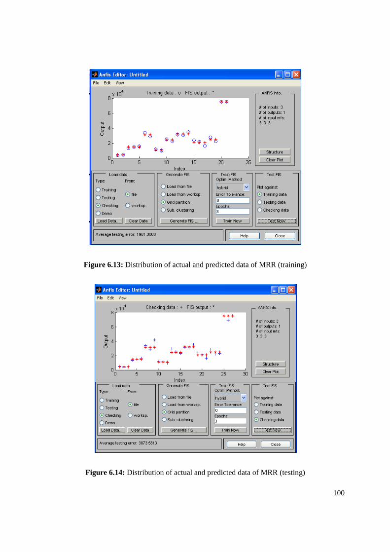
100

Figure 6.13: Distribution of actual and predicted data of MRR (training)

Figure 6.14: Distribution of actual and predicted data of MRR (testing)

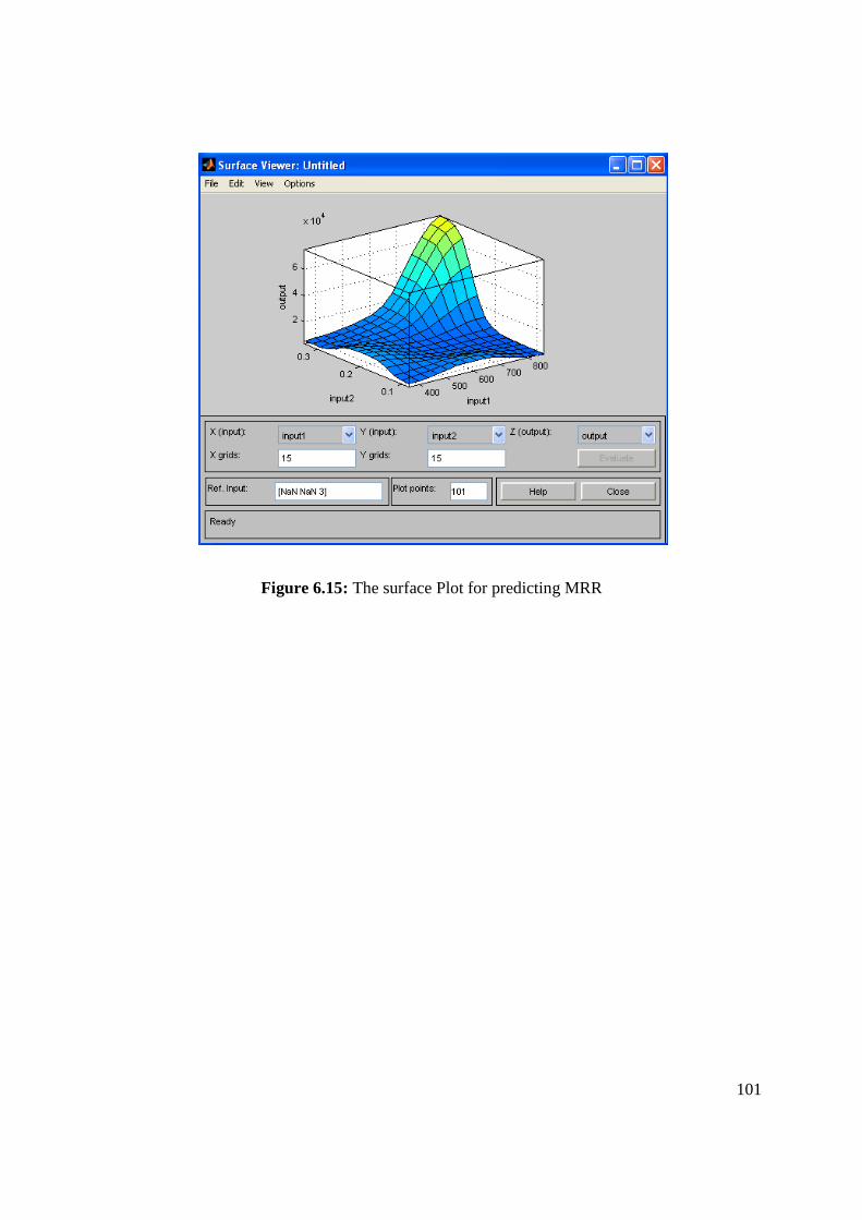
101

Figure 6.15: The surface Plot for predicting MRR

102

Chapter 7

Conclusion and Scope for Future Work

7.1 Conclusion

In the foregoing study, detailed investigation emphasizing process modeling along with multi-

response optimization has been attempted followed by a case study in composite machining.

Glass fiber reinforced polymers offer excellent machining properties in comparison with

conventional engineering materials. It has been revealed that various machining parameters have

certain degree of influence on surface roughness and material removal rate (MRR) during

machining operation. Quality and productivity are two important aspects of concern in

manufacturing/production industries. Improving quality-productivity by reducing cost and

increasing the performance of machine tools are indeed the challenging aspects in manufacturing

industries to survive competitively in the global marketplace. In general, among different

controllable process variables which are responsible in affecting process performances i.e.

process- responses (output); it is indeed very difficult to find the best optimal parameter settings.

The thesis aims to search the best process environment; simultaneously satisfying conflicting

requirements of process responses. Traditional, hybrid optimization methodologies have been

applied to search satisfactory results. The objectives of the thesis have been established

considering the scope in overcoming the limitations and trends of the single objective

optimization documented in literature.

In Chapter 3 application of TOPSIS based Taguchi method has been adopted to optimize

multiple surface roughness parameters of machined GFRP polyester composites. The concept of

this method is to select the alternative that have the shortest distance from the positive ideal

103

solution and the farthest distance from negative ideal solution. Positive ideal solution is a

solution that maximizes the benefit criteria and minimizes cost criteria, whereas the negative

ideal solution maximizes the cost criteria and minimizes the benefit criteria.

The above methodology explains the cost and time consuming effects which create errors. So, it

is necessary that the primary function of one intelligent technique is replaced by the primary

function of another intelligent technique to increase quality and productivity.

Application of desirability function, utility theory and fuzzy based Taguchi optimization method

has been presented in Chapter 4. Literature reveals that Taguchi approach fails to solve multi-

objective optimization problems. Various methodologies like desirability function, utility theory,

and grey theory have been attempted by previous researchers to find the optimal condition but

improper assignment of response weight and existence of correlation among the responses may

yield erroneous results. To avoid those limitations fuzzy logic has been integrated with the

aforesaid optimization philosophies.

In order to eliminate response correlation, application of PCA- fuzzy based Taguchi method has

been explained in Chapter 5. Principal Component Analysis (PCA) is one of the most useful

statistical techniques for examining the relationships within a given data set of multiple-

performance-characteristics. A new set of uncorrelated data, called principal components (PCs)

can be derived by PCA in descending order of their ability to explain the variance of the original

dataset. This uncorrelated quality responses are to be fed in Fuzzy Inference System (FIS) to

compute MPCI. MPCI is to be optimized by Taguchi method.

Chapter 6 shows one of the latest techniques i.e. application of ANFIS based prediction

modeling. The knowledge and the pattern are difficult to learn by the neural network. But fuzzy

logic models are easy to cover because they use linguistic terms in the form of IF-THEN rules. A

104

neural network with their learning capabilities can be used to learn the fuzzy decision rules, thus

creating a hybrid intelligent system i.e. ANFIS. The fuzzy system provides expert knowledge to

be used by the neural network. An efficient mathematical approach for the calculation of quality

and productivity indicator factors in turning operations has been studied. Surface roughness

average (Ra), Rq (root mean square roughness), Rt (Maximum Height of Profile) , Rsm (Mean

width of profile elements), Rku (Kurtosis of the roughness profile), Rz (Average Maximum Height

of the Profile) and material removal rate (MRR) are calculated as function of depth of cut, feed

rate, cutting speed.

The methodologies for prediction as well as optimization has been presented, the theoretical

studies on the surface roughness generation and the material removal rate would permit machine

tool operators to optimize the parameter selection, maximizing productivity while ensuring

quality requirements.

When a single set of experimentally measured data is analyzed by a number of computational

techniques with a unified aim (such as providing a set of optimum process conditions), it is felt

necessary to deliver a discussion and subsequent conclusion on the relative performance/measure

of the techniques that are used. To answer this, it is very difficult to conclude firmly on relative

performance of the optimization philosophies presented. It is very difficult to say which

technique is the most efficient. It mainly depends on the Decision-Maker (DM). The DM should

decide how many objective functions need to be considered, what will be the response priority

weight? Whether response correlation is to be considered or not? Moreover, depending of the

application area and functional requirements of the product, DM should think on criteria

requirements (Higher-the-Better/Lower-the-Better/Target-is-the-Best). The objective of the

thesis is to modify existing optimization philosophies to overcome inherent assumptions as well

105

as modifications. For example, TOPSIS/DF Approach/Utility Theory combined with Taguchi

method can be applied for uncorrelated multi-response optimization; whereas PCA/FIS based

Taguchi method can be used to optimize multiple correlated responses simultaneously.

Therefore, it is managerial decision (discretion of the Decision-Making group) towards selecting

a particular optimization tool/technique.

The main contributions of this research have been summarized below.

1. Development of PCA-Fuzzy-Taguchi integrated multi-objective optimization procedural

hierarchy applicable for continuous quality-productivity improvement and off-line quality

control in any manufacturing/production processes.

2. The proposed multi-objective optimization module is capable of overcoming

limitations/assumptions those are inherent in traditional Taguchi based optimization

techniques documented in literature.

3. Exploration of Fuzzy Inference System (FIS) avoids possibility of imprecision,

inaccuracy of prediction generally caused by improper assignment of response weights,

and existence of inter-correlation among output responses.

4. ANFIS modeling reveals behavioral scenario of process input parameters in relation with

output responses.

106

7.2 Scope for Future Work

The limitations of this research are as follows:

1. Interaction effect of process parameters has been neglected.

2. The composite with random fiber orientation has been studied only.

3. Variation of tool geometry, tool material has not been considered.

4. Effect of machine tool vibration has been ignored.

Some future directions of this research are as follows:

1. Investigation on machining of composites with a variety of fiber orientation.

2. Aspects of tool life/tool wear have to be investigated. In any kind of machining process,

another aspect of great concern is the tool life. Lesser extent of tool wear and increased

tool life is always preferred. The present work highlights quality-productivity

optimization in machining GFRP composites. Surface roughness values have been

considered as the product quality measure; and MMR has been interpreted as productivity

estimate. As tool life is not directly related to quality-productivity; therefore, this aspect

has not been considered/included in the list of objective functions.

3. Apart from turning, other machining processes like milling, drilling etc. need to be

carried out on composite materials.

4. Dimensional accuracy, extent tool wear may be included in the list of objective functions.

5. Apart from triangular fuzzy membership function, trapezoidal MFs may be explored.

107

Bibliography

1. M. Rahman, S. Ramakrishna, J.R.S. Prakash, D.C.G. Tan, Machinability study of carbon

fiber reinforced composite, Journal of Materials Processing Technology, 89-90 (1999)

292-297.

2. J. R. Ferreira, N.L. Coppini, G.W.A. Miranda, Machining Optimisation in Carbon Fibre

Reinforced Composite Materials, Journal of Materials Processing Technology, 92-93

(1999) 135-140.

3. E. Ugo. Enemuoh, A. Sherif El-Gizawy, A. Chukwujekwu Okafor, An Approach for

Development of Damage-Free Drilling of Carbon Fiber Reinforced Thermosets,

International Journal of Machine Tools and Manufacture, 41 (12) (2001) 1795-1814.

4. J. Paulo Davim, Pedro Reis, C. Conceição António, Experimental Study of Drilling Glass

Fiber Reinforced Plastics (GFRP) Manufactured by Hand Lay-Up, Composites Science

and Technology, 64 (2) (2004) 289-297.

5. I. El-Sonbaty, U.A. Khashaba, T. Machaly, Factors Affecting the Machinability of

GFR/Epoxy Composites, Composite Structures, 63 (2004) 329–338.

6. J. Paulo Davim, F. Mata, Optimisation of Surface Roughness on Turning Fibre-

Reinforced Plastics (FRPs) with Diamond Cutting Tools, International Journal of

Advanced Manufacturing Technology, 26 (2005a) 319–323.

7. J. Paulo Davim, F. Mata, A New Machinability Index in Turning Fiber Reinforced

Plastics, Journal of Materials Processing Technology, 170 (1-2) (2005b) 436-440.

8. R. Zitoune, F. Collombet, F. Lachaud, R. Piquet, P. Pasquet, Experiment–Calculation

Comparison of the Cutting Conditions Representative of the Long Fiber Composite

Drilling Phase, Composites Science and Technology, 65 (3-4) (2005) 455-466.

108

9. E. Bagci, B. Işık, Investigation of Surface Roughness in Turning Unidirectional GFRP

Composites by Using RS Methodology and ANN, International Journal of Advanced

Manufacturing Technology, 31 (2006) 10–17.

10. J. Paulo Davim, F. Mata, New Machinability Study of Glass Fibre Reinforced Plastics

Using Polycrystalline Diamond and Cemented Carbide (K15) Tools, Materials and

Design, 28 (3) (2007) 1050-1054.

11. C.C. Tsao, H. Hocheng, Evaluation of Thrust Force and Surface Roughness in Drilling

Composite Material Using Taguchi Analysis and Neural Network, Journal of Materials

Processing Technology, 203 (1-3) (2008) 342-348.

12. J. Campos Rubio, A.M. Abrao, P.E. Faria, A. Esteves Correia, J. Paulo Davim, Effects of

High Speed in the Drilling of Glass Fibre Reinforced Plastic: Evaluation of the

Delamination Factor, International Journal of Machine Tools and Manufacture, 48 (6)

(2008) 715-720.

13. Jamal Sheikh-Ahmad, R. Yadav, Model for Predicting Cutting Forces in Machining

CFRP, International Journal of Materials and Product Technology, 32 (2-3) (2008) 152-

167.

14. J. Paulo Davim, Leonardo R. Silva, António Festas, A.M. Abrão, Machinability Study on

Precision Turning of PA66 Polyamide With and Without Glass Fiber Reinforcing,

Materials and Design, 30 (2009) 228–234.

15. M. K. A Mohd Ariffin, M. I. Mohd Ali, S. M. Sapuan, N. Ismail, An Optimised Drilling

Process for an Aircraft Composite Structure Using Design of Experiments, Scientific

Research and Essay, 4 (10) (2009) 1109-1116.

16. António T. Marques, Luís M. Durão, António G. Magalhães, João Francisco Silva, João

Manuel R.S. Tavares, Delamination Analysis of Carbon Fibre Reinforced Laminates:

109

Evaluation of a Special Step Drill, Composites Science and Technology, 69 (14) (2009)

2376-2382.

17. F. Mata, E. Beamud, I. Hanafi, A. Khamlichi, A. Jabbouri,, M. Bezzazi, Multiple

Regression Prediction Model for Cutting Forces in Turning Carbon-Reinforced PEEK

CF30, Advances in Materials Science and Engineering, 2010 (2010), Article ID 824098,

7 pages, doi:10.1155/2010/824098.

18. G. Santhanakrishnan, R. Krishnamurthy, S.K. Malhotra, Machinability Characteristics of

Fibre Reinforced Plastics Composites, Journal of Mechanical Working Technology, 17

(1988) 195 – 204.

19. K.L. Palanikumar, R. Karunamoorthy, Kartikeyan, Optimizing of Machining Parameters

for Minimum Surface Roughness in Turning of GFRP Composites using Design of

Experiments, Journal of Materials Processing Technology, 20 (4) (2004) 373-378.

20. N.S. Mohan, A. Ramachandra, S.M. Kulkarni, Influence of Process Parameters on

Cutting Force and Torque during Drilling of Glass–Fiber Polyester Reinforced

Composites, Composite Structures, 71 (2005) 407–413.

21. N. Dayananda Jawali, B. Siddeswarappa, Siddaramaiah, Physicomechanical Properties,

Machinability, and Morphological Behavior of Short Glass Fiber-reinforced Nylon 6

Composites, Journal of Reinforced Plastics and Composites, 25 (13) (2006) 1409-1418.

22. K. Palanikumar, L. Karunamoorthy, R. Karthikeyan, Assessment of Factors Influencing

Surface Roughness on the Machining of Glass Fiber-Reinforced Polymer Composites,

Materials and Design, 27 (2006) 862–871.

23. K. Palanikumar, J. P. Davim, Mathematical Model to Predict Tool Wear on the

Machining of Glass Fiber Reinforced Plastic Composites, Materials and Design, 28

(2007) 2008–2014.

110

24. K. Palanikumar, Modeling and Analysis for Surface Roughness in Machining Glass Fibre

Reinforced Plastics Using Response Surface Methodology, Materials and Design, 28

(2007) 2611–2618.

25. S.R. Karnik, V.N. Gaitonde, Francisco Mata, J. Paulo Davim, Investigative Study on

Machinability Aspects of Unreinforced and Reinforced PEEK Composite Machining

using ANN Model, Journal of Reinforced Plastics and Composites, 27 (7) (2008) 751-

768.

26. K. Palanikumar, Application of Taguchi and Response Surface Methodologies for

Surface Roughness in Machining Glass Fiber Reinforced Plastics by PCD Tooling,

International Journal of Advanced Manufacturing Technology, 36 (2008a) 19–27.

27. Abeesh C. Basheer, Uday A. Dabade, Suhas S. Joshi, V.V. Bhanuprasad, V.M. Gadre,

Modeling of Surface Roughness in Precision Machining of Metal Matrix Composites

using ANN, Journal of Materials Processing Technology, 197 (2008) 439–444.

28. K. Palanikumar, F. Mata, J. Paulo Davim, Analysis of Surface Roughness Parameters in

Turning of FRP Tubes by PCD Tool, Journal of Materials Processing Technology, 204

(2008) 469–474.

29. K. Palanikumar, 2008b, Surface Roughness Model for Machining Glass Fiber Reinforced

Plastics by PCD Tool using Fuzzy Logics, Journal of Reinforced Plastics and

Composites, Vol. 00, No. 00/2008 1-14. DOI: 10.1177/0731684408092009.

30. V. Krishnaraj, Effect of Drill Points on Glass Fibre reinforced Plastics Composites while

Drilling at High Spindle Speed, Proceedings of the World Congress on Engineering,

Volume II, WCE 2008, July 2-4, 2008, London, U.K.

31. A. Naveen Sait, S. Aravindan, A. Noorul Haq, Optimization of Machining Parameters of

Glass Fiber Reinforced Plastic (GFRP) Pipes by Desirability Function Analysis using

111

Taguchi Technique”, International Journal of Advance Manufacturing Technology, 43

(2009) 581-589.

32. K. Palanikumar, J. P. Davim, Assessment of Some Factors Influencing Tool Wear on the

Machining of Glass Fiber Reinforced Plastics by Coated Cemented Carbide Tools,

Journal of Materials Processing and Technology, 209 (2009) 511–519.

33. R. Vimal Sam Singh, B. Latha, V.S. Senthikumar, Modeling and Analysis of Thrust

Force and Torque in Drilling GFRP Composites by Multi-Facet Drill Using Fuzzy Logic,

International Journal of Recent Trends in Engineering, 1 (5) (2009) 66-70.

34. S.A. Hussain, V. Pandurangadu, K. Palanikumar, Surface Roughness Analysis in

Machining of GFRP Composites by Carbide Tool (K20), European Journal of Scientific

Research, 41 (1) (2010) 84-98.

35. T. Rajasekaran, K. Palanikumar, B.K. Vinayagam, Application of Fuzzy Logic for

Modeling Surface Roughness in Turning CFRP Composites Using CBN Tool, Production

Engineering and Research Development, 5 (2011) 191-199.

36. G. Spur, U.E. Wunsch, Turning of fiber-reinforced plastics, Manuf Rev, (1998), 1(2)

124–129.

37. O.B. Abouelatta, J. M´adl, Surface roughness prediction based on cutting parameters and

tool vibrations in turning operations. Journal of Materials Processing Technology,

118(2001) 269–277.

38. E. Erisken, Influence from production parameters on the surface roughness of a machine

short fibre reinforced thermoplastic, International Journal of Machine Tools and

Manufacture, 39(1999) 1611–1618.

39. F. Mata, J.P. Davim, An investigation about the precision turning fiber reinforced plastics

(FRP’s) with diamond cutting tools using multiple analysis regression. II Iberian

Conference of Tribology, (2003), Valencia, pp. 117–124.

112

40. S. Jahanmir, M. Ramulu, P. Koshy, Machining of ceramics and composites. Dekker, New

York, (1998) 238–243.

41. V.K. Jain, S.K. Choudhury, K.M. Ramesh, On the machining of alumina and glass,

International Journal of Machine Tools and Manufacture, 42(2002) 1269–1276.

42. J.P. Davim, Silva Leonardo R, F. António, A.M. Abrão, Machinability study on precision

turning of PA66 polyamide with and without glass fiber reinforcing, Materials and

Design, 30(2009) 228–34.

43. M.H. Geier, Quality handbook for composite materials. Chapman & Hall Publications;

1994.

44. E.S. Lee, Precision machining of glass fibre reinforced plastics with respect to tool

characteristics, International Journal of Advanced Manufacturing Technology, 17(2001)

791–8.

45. L.C. Zhang, Cutting composites: a discussion on mechanics modeling, Journal of

Materials Processing Technology, 209(2009) 4548–52.

46. G. Santhanakrishnan, R. Krishnamurthy, S.K. Malhotra, High speed tool wear studies in

machining of glass fibre reinforced plastic, Wear, 132(1989) 327–336.

47. N. Bhatnagar, N. Ramakrishnan, N.K. Naik, R. Komanduri, On the machining of fibre

reinforced plastic (FRP) composite laminates, International Journal of Machine Tools and

Manufacture, 35(5)(1995) 701–16.

48. Venu Gopala Roa G, P. Mahajan, N. Bhatnagar, Machining of UD—GFRP composites

chip formation mechanism, Composites Science and Technology, 67(2007) 2271–81.

49. M. Sharma, I.M. Rao, J. Bijwe, Influence of orientation of long fibers in carbon fiber–

polyetherimide composites on mechanical and tribological properties, Wear, 267(2009)

839–45.

113

50. P.S. Sreejith, R. Krishnamurthy, S.K. Malhotra, Effect of specific cutting pressure and

temperature during machining of carbon/phenolic ablative composite using PCBN tools,

Journal of Materials Processing Technology, 183(2007) 88–95.

51. Syed Altaf Hussain, V. Pandurangadu, K. Palanikumar, Surface Roughness Analysis in

Machining of GFRP Composites by Carbide Tool (K20), European Journal of Scientific

Research, 41(1)(2010) 84-98.

52. P. Sahoo, Engineering Tribology, Prentice Hall of India, New Delhi, 2005.

53. S. Datta, A. Bandyopadhyay, P.K. Pal, Application of Taguchi Philosophy for Parametric

Optimization of Bead Geometry and HAZ Width in Submerged Arc Welding Using

Mixture of Fresh Flux and Fused Slag, International Journal of Advanced Manufacturing

Technology, 36 (2008a) 689-698.

54. S. Datta, A. Bandyopadhyay, P.K. Pal, Grey Based Taguchi Method for Optimization of

Bead Geometry in Submerged Arc Bead-On-Plate Welding, International Journal of

Advanced Manufacturing Technology, 39 (2008b) 1136-1143.

55. G. Derringer, R. Suich, Simultaneous optimization of several response variables, Journal

of Quality Technology, 12 (4) (1980) 214-219.

56. S. Datta, A. Bandyopadhyay, P. K. Pal, Desirability Function Approach for Solving

Multi-Objective Optimization Problem in Submerged Arc Welding, International Journal

for Manufacturing Science and Production, 7(2) (2006) 127-135.

57. P. Kumar, P. B. Barua, J. L. Gaindhar, Quality Optimization (Multi-Characteristics)

Through Taguchi’s Technique and Utility Concept, Quality and Reliability Engineering

International, 16 (2000) 475-485.

58. R. S. Walia, H. S. Shan, P. Kumar, Multi-Response Optimization of CFAAFM Process

through Taguchi Method and Utility Concept, Materials and Manufacturing Processes, 21

(2006) 907-914.

114

59. S. Datta, G. Nandi, A. Bandyopadhyay, Application of Entropy Measurement Technique

in Grey Based Taguchi Method for Solution of Correlated Multiple Response

Optimization Problems: A Case Study in Welding, Journal of Manufacturing Systems, 28

(2009a) 55-63.

60. C.T. Su, L.I. Tong, Multi-Response Robust Design by Principal Component Analysis,

Total Quality Management, 8 (6) (1997) 409-416.

61. S. Datta, G. Nandi, A. Bandyopadhyay, P. K. Pal, Application of PCA based hybrid

Taguchi method for multi-criteria optimization of submerged arc weld: A case study,

International Journal of Advanced Manufacturing Technology, 45 (3-4) (2009b) 276-286.

62. B. C. Routara, S. D. Mohanty, S. Datta, A. Bandyopadhyay, S. S. Mahapatra, Combined

Quality Loss (CQL) concept in PCA based Taguchi philosophy for optimization of

multiple surface quality characteristics of UNS C34000 Brass in cylindrical grinding,

International Journal of Advanced Manufacturing Technology, 51 (2010) 135-143.

63. Hung-Chang Liao, Multi-Response Optimization Using Weighted Principal Component,

International Journal of Advanced Manufacturing Technology, 27 (7-8) (2006) 720-725.

64. D. Lu, J. Antony, Optimization of Multiple Responses Using a Fuzzy-Rule Based

Inference System, International Journal of Production Research, 40 (7) (2002) 1613-1625.

65. L.A. Zadeh, Fuzzy-Algorithm Approach to the Definition of Complex or Imprecise

Concept, International Journal of Man Machine Studies, 8 (1976) 249-291.

66. J.M. Mendel, Fuzzy Logic Systems for Engineering: A Tutorial, IEEE Proc, 83 (1995)

345-377.

67. E.A. Cox, Fuzzy Fundamentals, IEEE Spectrum, 29 (1992) 58-61.

68. R.R. Yager, D.P. Filev, Essential of Fuzzy Modeling and Control, 1999, John Willey and

Sons Inc., New York.

115

69. P.J. Ross, Taguchi Techniques for Quality Engineering: Loss Function, Orthogonal

Experiments, Parameter and Tolerance Design - 2nd ed, New York, NY: McGraw-Hill

(1996).

70. M.S. Phadke, Quality Engineering Using Robust Design. Englewood Cliffs, NJ: Prentice-

Hall; (1989).

71. W.H. Yang, Y.S. Tarng, Design optimization of cutting parameters for turning operations

based on the Taguchi method, Journal of Materials Processing Technology, 84 (1998)

122–129.

72. Y.L. Su, S.H. Yao, C.S. Wei, W.H. Kao , C.T. Wu, Design and performance analysis of

TiCN- coated cemented carbide milling cutters, Journal of Materials Processing

Technology, 87 (1999) 82–89.

73. C.Y. Nian, W.H. Yang, Y. S. Tarng, Optimization of turning operations with multiple

performance characteristics, Journal of Materials Processing Technology, 95 (1999) 90–

96.

74. T.R. Lin, Experimental design and performance analysis of TiN coated carbide tool in

face milling stainless steel, Journal of Materials Processing Technology, 127 (2002) 1–7.

75. J.P. Davim, Design optimization of cutting parameters for turning metal matrix

composites based on the orthogonal arrays, Journal of Materials Processing Technology,

132 (2003) 340–344.

76. J.A. Ghani, I.A. Choudhury , H.H. Hassan, Application of Taguchi method in the

optimization of end milling operations, Journal of Materials Processing Technology, 145

(2004) 84–92.

77. C. L. Hwang, K. Yoon, ‘Multiple Attribute Decision Making Methods and Applications’,

A State-of-the-Art Survey, Springer Verlag, New York (1981).

116

78. L.-I. Tong, C.-T. Su, Optimizing multi-response problems in the Taguchi method by

fuzzy multiple attribute decision making, Quality and Reliability Engineering

International 13 (1997) 25–34.

79. Liao Hung-Chang, Using PCR-TOPSIS to optimize Taguchi’s multi-response problem,

International Journal of Advanced Manufacturing Technology, 22 (2003) 649-655.

80. Y. Wang, Z. He, A New TOPSIS Based Methodology for Multiple Responses Problem,

8th International Conference on Wireless Communications, Networking and Mobile

Computing WiCOM, Dalian (2008).

81. C.T. Su, L.I. Tong, Multi-Response Robust Design by Principal Component Analysis,

Total Quality Management, 8 (6) (1997) 409-416.

82. Sivarao, P. Brevern, N.S.M. El-Tayeb, V.C. Vengkatesh, Mamdani fuzzy inference

system modeling to predict surface roughness in laser machining. International Journal of

Intelligent Information and Technology Application, 2(1) (2009) 12-18.

83. Yi-Chin Fang, Yih-Fong Tzeng, Si-Xiang. Li, A Taguchi PCA fuzzy-based approach for

the multi-objective extended optimization of a miniature optical engine Journal of Physics

D: Applied Physics, 41(17) (2008) 16.

84. M. Sugeno, G.T. Kang, Structure identification of fuzzy model. Fuzzy Sets System, 28

(1988) 15–33.

85. R. J. Jang, Fuzzy modeling using generalized neural networks and Kalmman filter

algorithm. In Proceedings of the ninth national conference on artificial intelligence,

(1991) 762–767.

86. R.J. Jang, ANFIS: Adaptive-network-based fuzzy inference system. IEEE Transaction on

Systems of Max and Cybernatics, 23(03) (1993) 665–685.

87. J. S. Roger Jang and C. T. Sun, “Neuro-fuzzy modeling and control”, Proceedings of the

IEEE, 83, pp. 378 –404, 1995.

117

88. C. L. Hwang, K. Yoon, Multiple Attribute Decision Making Methods and Applications, A

State-of-the-Art Survey, Springer Verlag, New York, (1981).

89. T. S. Lan, Taguchi Optimization of multi- objective CNC Machining using TOPSIS,

Information Technology Journal, 86 (2009) 917-922.

90. T. Yang, P. Chou, Solving a multiresponse simulation-optimization problem with discrete

variables using a multiple-attribute decision-making method, Mathematics and

Computers in Simulation,68 (2005) 9-21.

91. E.Angun, G. Gurkan, D. Hertog, J. P. C. Kleijnen, Response surface methodology with

stochastic constraints for expensive simulation, Working Paper, Tilburg University,

Netherlands, (2003).

92. L.-I. Tong, C.-T. Su, Optimizing multi-response problems in the Taguchi method by

fuzzy multiple attribute decision making, Quality and Reliability Engineering

International, 13 (1997) 25-34.

93. Y. Wang, Z. He, Optimal Multi-response Problems on the Improved TOPSIS Method,

Wireless Communications, networking and Mobile Computing, (2007) 5092-5094.

94. P. Liu, An Extended TOPSIS Method for Multiple Attribute Group Decision Making

Based on Generalized Interval-valued Trapezoidal Fuzzy Numbers, Informatica, 35

(2011) 185-196.

95. W. H. Yang, Y. S. Tang, Design optimization of cutting parameters for turning operations

based on the Taguchi method, Journal of Material Processing and Technology, 84 (1998)

122-129.

96. H. S. Adeel, N. Ismail, S. V. Wong, J. N.A. Abdul, Optimization of Cutting Parameters

Based on Surface Roughness and Assistance of Work piece Surface Temperature in

Turning Process, American Journal of Engineering and Applied Sciences, 3 (1) (2010)

102-108.

118

97. S. A. Hussain, V. Pandurangadu, K. Palanikumar, Surface Roughness Analysis in

Machining of GFRP Composites by Carbide Tool (K20), European Journal of Scientific

Research, 41 (1) (2010) 84-98.

98. A. Singh, S. Datta, S. S. Mahapatra, T. Singha, G. Majumdar, Optimization of Bead

Geometry of Submerged Arc Weld using Fuzzy based Desirability Function Approach,

Journal of Intelligent Manufacturing, Springer link. (Published Online 21 April 2011)

DOI 10.1007/s10845-011-0535-3 (2011).

99. A. Azadeh, M. Seifoory, M. Abbasi, Integration of simulation and fuzzy multi-attribute

decision making for modeling and assessment of fuzzy parameters, International Journal

of Industrial and Systems Engineering, 6 (4) (2010) 483-502.

100. M. Kumar, S.P. Yadav, S. Kumar, A new approach for analyzing the fuzzy system

reliability using intuitionistic fuzzy number, International Journal of Industrial and

Systems Engineering, 8 (2) (2011) 135-156.

101. Y.M. Ali, L.C. Zhang, Surface roughness prediction of ground components using a

fuzzy logic approach, Journal of Materials Processing Technology, 89–90 (1999) 561–

568.

102. A. Gupta, H. Singh, A. Aggarwal, Taguchi-fuzzy multi output optimization (MOO) in

high speed CNC turning of AISI P-20 tool steel, Expert Systems with Applications, 38

(2011), 6822–6828.

103. J.-S. R. Jang, ANFIS: Adaptive-Network-Based Fuzzy Inference System, Systems,

Man and Cybernetics, 23(3) (1993) 665–685.

104. Y. Jiao, S. Lei, Z.J. Pei, E.S. Lee, Fuzzy Adaptive Networks in process modeling:

surface roughness prediction for turning operations, International Journal of Machine

Tools and Manufacture, 44(15) (2004) 1643–1651.

119

105. J.C. Chen, M. Savage, A fuzzy-net based multi level in Process surface roughness

recognition system in milling operation, International Journal of Advanced

Manufacturing Technology, 17 (2001) 670–676.

106. S.J. Lou, J.C. Chen, In-Process surface roughness recognition (ISSR) system in end-

milling operation, International Journal of Advanced Manufacturing Technology, 15

(1999) 200–209.

107. B. Lin, M.Z. Zhu, S.Y. Yu, H.T. Zhu, M.X. Lin, Study of synthesis identification in

the cutting process with a fuzzy neural network, Journal of Materials Processing

Technology, 129 (2002) 131–134.

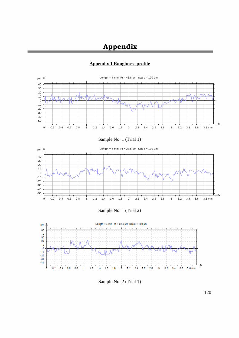
120

Appendix

Appendix 1 Roughness profile

µm

-50

-40

-30

-20

-10

0

10

20

30

40

0 0.2 0.4 0.6 0.8 1 1.2 1.4 1.6 1.8 2 2.2 2.4 2.6 2.8 3 3.2 3.4 3.6 3.8 mm

Length = 4 mm Pt = 46.8 µm Scale = 100 µm

Sample No. 1 (Trial 1)

µm

-50

-40

-30

-20

-10

0

10

20

30

40

0 0.2 0.4 0.6 0.8 1 1.2 1.4 1.6 1.8 2 2.2 2.4 2.6 2.8 3 3.2 3.4 3.6 3.8 mm

Length = 4 mm Pt = 38.5 µm Scale = 100 µm

Sample No. 1 (Trial 2)

Sample No. 2 (Trial 1)

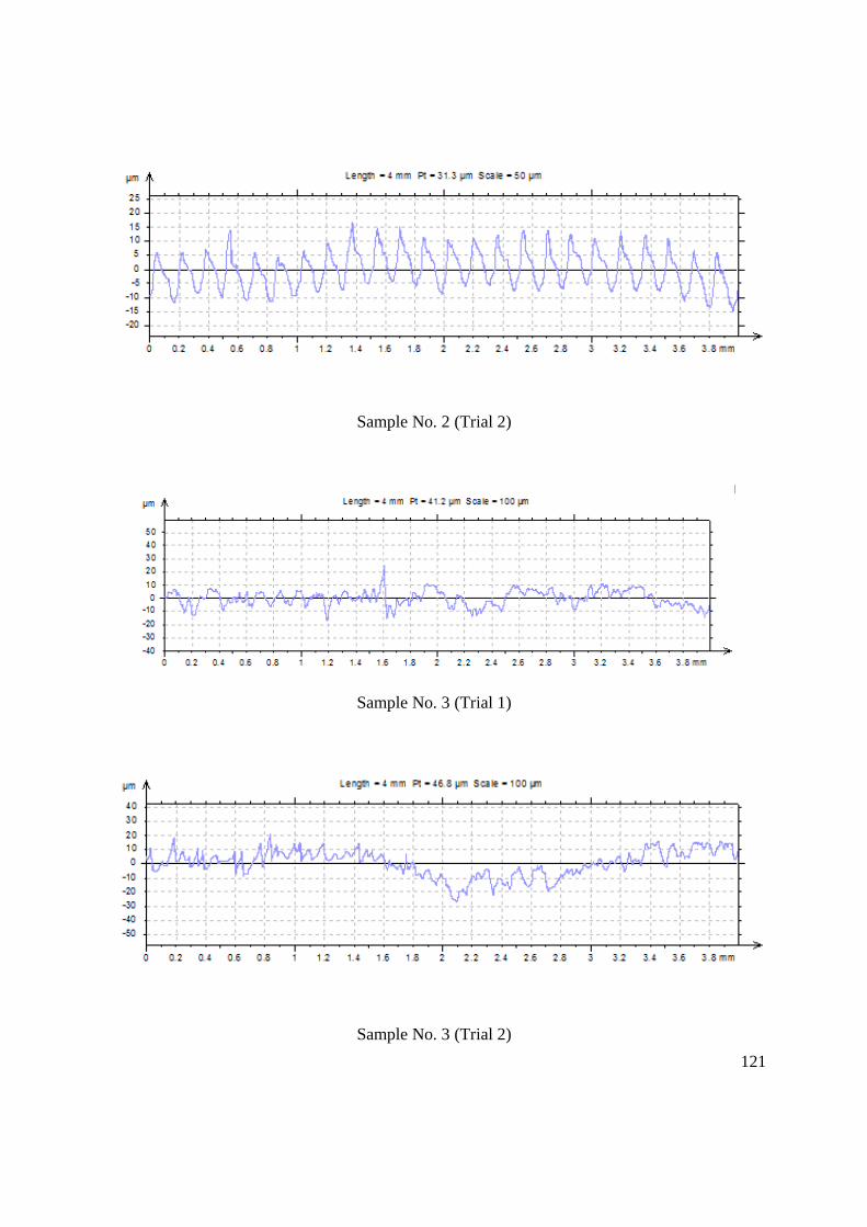
121

Sample No. 2 (Trial 2)

Sample No. 3 (Trial 1)

Sample No. 3 (Trial 2)

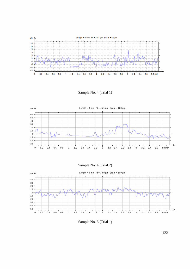
122

Sample No. 4 (Trial 1)

µm

-30

-20

-10

0

10

20

30

40

50

60

0 0.2 0.4 0.6 0.8 1 1.2 1.4 1.6 1.8 2 2.2 2.4 2.6 2.8 3 3.2 3.4 3.6 3.8 mm

Length = 4 mm Pt = 45.1 µm Scale = 100 µm

Sample No. 4 (Trial 2)

µm

-50

-40

-30

-20

-10

0

10

20

30

40

0 0.2 0.4 0.6 0.8 1 1.2 1.4 1.6 1.8 2 2.2 2.4 2.6 2.8 3 3.2 3.4 3.6 3.8 mm

Length = 4 mm Pt = 33.8 µm Scale = 100 µm

Sample No. 5 (Trial 1)

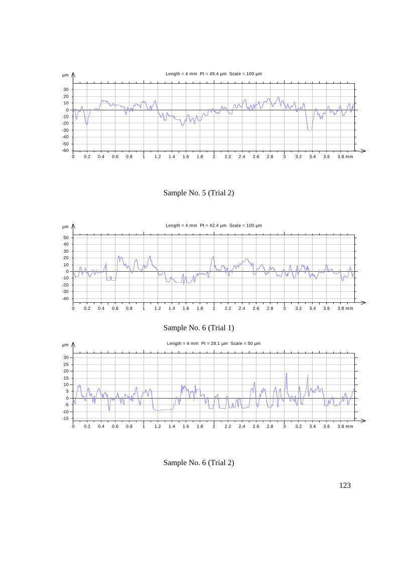
123

µm

-60

-50

-40

-30

-20

-10

0

10

20

30

0 0.2 0.4 0.6 0.8 1 1.2 1.4 1.6 1.8 2 2.2 2.4 2.6 2.8 3 3.2 3.4 3.6 3.8 mm

Length = 4 mm Pt = 49.4 µm Scale = 100 µm

Sample No. 5 (Trial 2)

µm

-40

-30

-20

-10

0

10

20

30

40

50

0 0.2 0.4 0.6 0.8 1 1.2 1.4 1.6 1.8 2 2.2 2.4 2.6 2.8 3 3.2 3.4 3.6 3.8 mm

Length = 4 mm Pt = 42.4 µm Scale = 100 µm

Sample No. 6 (Trial 1)

µm

-15

-10

-5

0

5

10

15

20

25

30

0 0.2 0.4 0.6 0.8 1 1.2 1.4 1.6 1.8 2 2.2 2.4 2.6 2.8 3 3.2 3.4 3.6 3.8 mm

Length = 4 mm Pt = 28.1 µm Scale = 50 µm

Sample No. 6 (Trial 2)

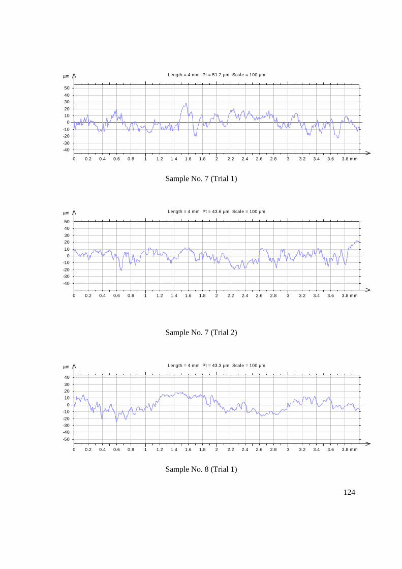
124

µm

-40

-30

-20

-10

0

10

20

30

40

50

0 0.2 0.4 0.6 0.8 1 1.2 1.4 1.6 1.8 2 2.2 2.4 2.6 2.8 3 3.2 3.4 3.6 3.8 mm

Length = 4 mm Pt = 51.2 µm Scale = 100 µm

Sample No. 7 (Trial 1)

µm

-40

-30

-20

-10

0

10

20

30

40

50

0 0.2 0.4 0.6 0.8 1 1.2 1.4 1.6 1.8 2 2.2 2.4 2.6 2.8 3 3.2 3.4 3.6 3.8 mm

Length = 4 mm Pt = 43.6 µm Scale = 100 µm

Sample No. 7 (Trial 2)

µm

-50

-40

-30

-20

-10

0

10

20

30

40

0 0.2 0.4 0.6 0.8 1 1.2 1.4 1.6 1.8 2 2.2 2.4 2.6 2.8 3 3.2 3.4 3.6 3.8 mm

Length = 4 mm Pt = 43.3 µm Scale = 100 µm

Sample No. 8 (Trial 1)

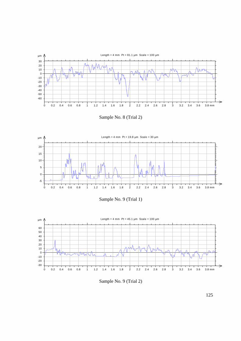
125

µm

-60

-50

-40

-30

-20

-10

0

10

20

30

0 0.2 0.4 0.6 0.8 1 1.2 1.4 1.6 1.8 2 2.2 2.4 2.6 2.8 3 3.2 3.4 3.6 3.8 mm

Length = 4 mm Pt = 81.1 µm Scale = 100 µm

Sample No. 8 (Trial 2)

µm

-5

0

5

10

15

20

0 0.2 0.4 0.6 0.8 1 1.2 1.4 1.6 1.8 2 2.2 2.4 2.6 2.8 3 3.2 3.4 3.6 3.8 mm

Length = 4 mm Pt = 19.8 µm Scale = 30 µm

Sample No. 9 (Trial 1)

µm

-30

-20

-10

0

10

20

30

40

50

60

0 0.2 0.4 0.6 0.8 1 1.2 1.4 1.6 1.8 2 2.2 2.4 2.6 2.8 3 3.2 3.4 3.6 3.8 mm

Length = 4 mm Pt = 45.1 µm Scale = 100 µm

Sample No. 9 (Trial 2)

126

Appendix 2 Definitions of various surface roughness features and MRR

1. Ra (arithmetic average height)

Roughness average Ra is the arithmetic average of the absolute values of the roughness profile

ordinates. Ra is the arithmetic mean roughness value from the amounts of all profile values.

( ) dxXZl

Rl

a ∫=0

1

2. Rq (root mean square roughness)

Root mean square (RMS) roughness Rq is the root mean square average of the roughness profile

ordinates. Rq is more sensitive to peaks and valleys then Ra, because the amplitudes are squared.

( ) dxXZl

Rl

q ∫=0

21

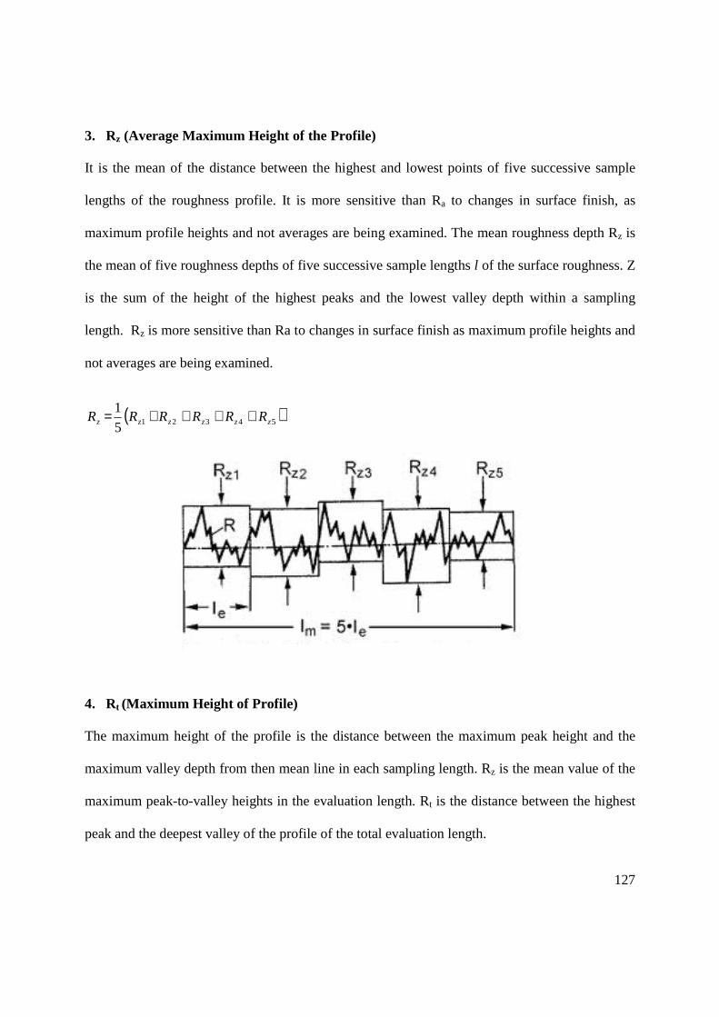
127

3. Rz (Average Maximum Height of the Profile)

It is the mean of the distance between the highest and lowest points of five successive sample

lengths of the roughness profile. It is more sensitive than Ra to changes in surface finish, as

maximum profile heights and not averages are being examined. The mean roughness depth Rz is

the mean of five roughness depths of five successive sample lengths l of the surface roughness. Z

is the sum of the height of the highest peaks and the lowest valley depth within a sampling

length. Rz is more sensitive than Ra to changes in surface finish as maximum profile heights and

not averages are being examined.

( )543215

1zzzzzz RRRRRR ++++=

4. Rt (Maximum Height of Profile)

The maximum height of the profile is the distance between the maximum peak height and the

maximum valley depth from then mean line in each sampling length. Rz is the mean value of the

maximum peak-to-valley heights in the evaluation length. Rt is the distance between the highest

peak and the deepest valley of the profile of the total evaluation length.

128

5. Rsm (Mean width of profile elements)

It is the arithmetic mean value of the widths of the profile elements of the roughness profile,

where a profile element is a peak and valley in the roughness profile. The units of Rsm are

micrometers or micro inches.

= ∑n

imism S

nR

1

129

6. Rku (Kurtosis of the roughness profile)

It is the quotient of the mean quadratic value of the ordinate value he fourth power of the Pq,

Rq, or Wq respectively, with in a sampling length. It is measure of sharpness of the probability

density function of the ordinate value.

∑=

=N

jj

q

ku rNR

R1

44

1

7. Material Removal Rate (MRR)

Material removal rate (MRR) has been calculated from the difference in weights of the work

pieces before and after experiment.

m

fi

t

WWMRR

.ρ−

= ( )min3mm

Here, iW is the initial weight of the work piece in gm

fW is the final weight of the work piece in gm

ρ is the density of work material (2 gm/cm3 for GFRP polyester) and

mt is the machining time in minute.

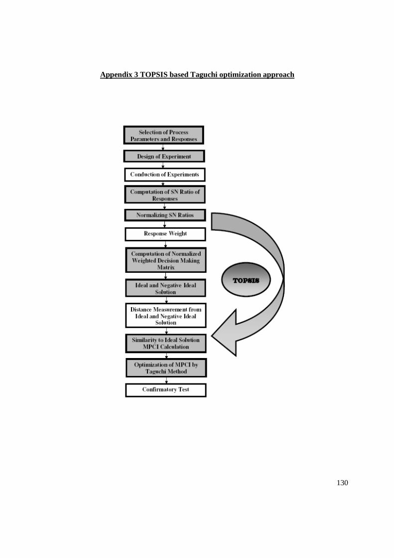
130

Appendix 3 TOPSIS based Taguchi optimization approach

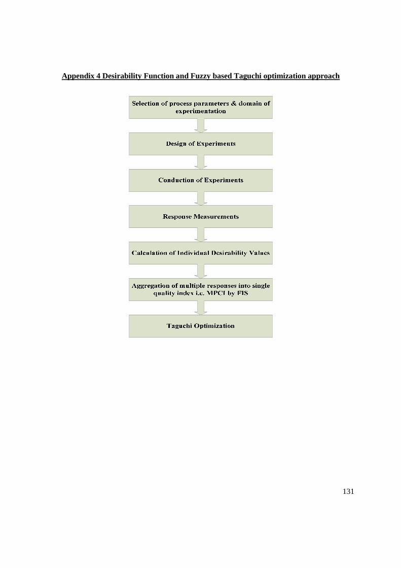
131

Appendix 4 Desirability Function and Fuzzy based Taguchi optimization approach

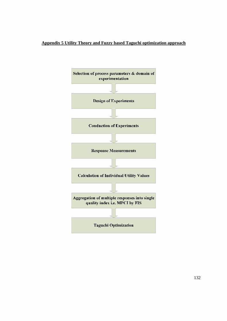
132

Appendix 5 Utility Theory and Fuzzy based Taguchi optimization approach

133

Appendix 6 PCA Fuzzy based Taguchi optimization approach

134

List of Publications

Journals

1. Ankita Singh, Saurav Datta, Siba Sankar Mahapatra, “Application of TOPSIS in the

Taguchi Method for Optimal Machining Parameter Selection”, 2011, Journal for Manufacturing Science and Production (JMSP), Vol. 11, pp. 49-60, De Gruyter, Germany.

2. Ankita Singh, Saurav Datta, Siba Sankar Mahapatra, “Principal Component Analysis and Fuzzy Embedded Taguchi Approach for Multi-Response Optimization in Machining of GFRP Polyester Composites: A Case Study”, International Journal of Industrial and Systems Engineering (IJISE), Inderscience Publishers. (In Press)

Conferences

3. Ankita Singh, Saurav Datta, Siba Sankar Mahapatra, “Application of PCA Based Fuzzy Reasoning Combined with Taguchi’s Philosophy In Machining of GFRP Polyester Composites”, Proceedings of the International Conference on Industrial Applications of Soft Computing Techniques (IIASCT 2011), August 20-22, 2011, Bhubaneswar, Orissa.

4. Ankita Singh, Ankita Sahu, Saurav Datta, Siba Sankar Mahapatra, “Aggregation of Multi-responses in Turning Process Optimization on GFRP (Polyester) Composite Using Utility-Fuzzy Approach”, 2nd National Conference on Recent Advances in Manufacturing (RAM-2011), 15-17 September 2011, Organized by Department of Mechanical Engineering, SV National Institute of Technology, Surat-395007.

5. Ankita Singh, Saurav Datta, Siba Sankar Mahapatra, “Multi-Objective Optimization of GFRP Composite Using Desirability Function based Fuzzy Approach Coupled with Taguchi Method”, International Conference on Advances in Supply Chain and Manufacturing Management, Achieving Growth, Profitability and Sustainability in a Globalized Environment (ASCMM 2011), December 16-18, 2011, organized by Department of Industrial Engineering and Management, Indian Institute of Technology, Kharagpur.

6. Ankita Singh, Kumar Abhishek, Jambeswar Sahu, Saurav Datta, Siba Sankar Mahapatra, “DEA based Taguchi Approach for Multi-Objective Optimization: A Case Study”, International Conference on Modeling, Optimization and Computing (ICMOC 2012), Noorul Islam University, Noorul Islam Centre for Higher Education, Kumaracoil, Thuckalay, Kanyakumari District, Tamilnadu State, India- 629 180, April 10-11 2012.