Embed Size (px)
Citation preview
HAL Id: tel-01764942https://pastel.archives-ouvertes.fr/tel-01764942
Submitted on 12 Apr 2018
HAL is a multi-disciplinary open accessarchive for the deposit and dissemination of sci-entific research documents, whether they are pub-lished or not. The documents may come fromteaching and research institutions in France orabroad, or from public or private research centers.
L’archive ouverte pluridisciplinaire HAL, estdestinée au dépôt et à la diffusion de documentsscientifiques de niveau recherche, publiés ou non,émanant des établissements d’enseignement et derecherche français ou étrangers, des laboratoirespublics ou privés.
Study and modeling of separation methods H2S frommethane, selection of a method favoring H2S valorization
Hamadi Cherif
To cite this version:Hamadi Cherif. Study and modeling of separation methods H2S from methane, selection of a methodfavoring H2S valorization. Chemical and Process Engineering. Université Paris sciences et lettres,2016. English. �NNT : 2016PSLEM074�. �tel-01764942�
Soutenue par Hamadi CHERIF le 08 Décembre 2016 h
Dirigée par Christophe COQUELET Paolo STRINGARI
h
COMPOSITION DU JURY :
M. Vincent GERBAUD Chemical Engineering Laboratory of Toulouse, Président
M. Eric MAY University of Western Australia, Rapporteur
Mme. Laura PELLEGRINI Politecnico di Milano, Examinatrice
M. Denis CLODIC Société Cryo Pur, Examinateur
M. Christophe COQUELET Mines ParisTech, Examinateur
M. Paolo STRINGARI Mines ParisTech, Examinateur
M. Joseph TOUBASSY Société Cryo Pur, Invité
Ecole doctorale n°432
SCIENCES DES METIERS DE L’INGENIEUR
Spécialité ENERGETIQUE ET GENIE DES PROCEDES
Etude et modélisation de méthodes de séparation du méthane et de H2S
Study and modeling of separation methods of H2S from methane
THÈSE DE DOCTORAT
de l’Université de recherche Paris Sciences et Lettres PSL Research University
Préparée à MINES ParisTech

2

3
Acknowledgements
I am grateful to Prof. Denis Clodic, supervisor of this thesis for the suggestions that helped to shape
my research skills and for the responsibility he granted to me. Without him, this dissertation would
not have been possible.
I would like to thank my supervisors Prof. Christophe Coquelet and Dr. Paolo Stringari, for their
continuous support, excellent supervision and guidance. Without them, this thesis would not have
been possible.
I express my gratitude to Prof. Eric May from the University of Western Australia and Prof. Vincent
Gerbaud from the Chemical Engineering Laboratory of Toulouse, for their patience while reading this
thesis.
I would like to thank Prof. Laura Pellegrini for her hospitality and disponibility during my stay in
Politecnico di Milano within "Group on Advanced Separation Processes & GAS Processing". It was an
opportunity to grow on both a personal and professional level.
I would also thank Dr. Joseph Toubassy, project leader at Cryo Pur Company, for being interested in
my work, for the various disscussion we had and for his technical aid.
I thank all the staff in CTP and Cryo Pur Company for their presene, their support and their advices.
I would like to recognize the support of my parents Jaafar and Wassila through all these years.
4
Table of contents
Abstract ............................................................................................. Erreur ! Signet non défini.
Nomenclature ............................................................................................................................. 7
List of figures .............................................................................................................................. 9
List of tables ............................................................................................................................. 11
General introduction ................................................................................................................ 13
Chapter 1: From biogas to biomethane ................................................................................... 17
1.1. Introduction ........................................................................................................................... 18
1.2. Biogas utilization ................................................................................................................... 19
1.2.1. Direct combustion ......................................................................................................... 19
1.2.2. Combined heat and power ............................................................................................ 19
1.2.3. Injection into the natural gas grid ................................................................................. 19
1.2.4. Vehicle fuel .................................................................................................................... 19
1.3. Biogas composition ............................................................................................................... 20
1.3.1. Household and industrial waste .................................................................................... 20
1.3.2. Sludge from sewage water treatment plants ................................................................ 21
1.3.3. Agricultural and agro-industrial waste .......................................................................... 21
1.4. Environmental and economic issues ..................................................................................... 23
1.5. From biogas to liquid biomethane ........................................................................................ 24
1.6. Conclusion ............................................................................................................................. 25
Chapter 2: Thermodynamic aspects of biogas ......................................................................... 26
2.1. Introduction ........................................................................................................................... 26
2.2. Thermodynamic properties of pure component present in biogas ...................................... 27
2.2.1. Hydrogen sulfide ........................................................................................................... 27
2.2.2. Carbon dioxide............................................................................................................... 28
2.2.3. Methane ........................................................................................................................ 29
2.3. Thermodynamic properties of the gas mixture (biogas) ................................................... 32
2.3.1. Phase equilibrium behavior of biogas ........................................................................... 32
2.3.2. Density and dynamic viscosity of biogas ....................................................................... 34
2.3.3. Thermal conductivity of biogas ..................................................................................... 35
2.3.4. Thermal capacities ......................................................................................................... 36
2.4. Energy content in biogas ....................................................................................................... 38

5
2.5. Conclusion ............................................................................................................................. 38
Chapter 3: From molecules to the process .............................................................................. 39
3.1. Introduction ........................................................................................................................... 39
3.2. Absorption technology .......................................................................................................... 40
3.2.1. Physical solvents ............................................................................................................ 41
3.2.2. Chemical solvents .......................................................................................................... 44
3.2.3. Hybrid solvents .............................................................................................................. 47
3.2.4. Gas-liquid contactors ..................................................................................................... 47
3.3. Adsorption technology .......................................................................................................... 50
3.3.1. Mechanism of adsorption ............................................................................................. 51
3.3.2. Materials used for H2S adsorption ................................................................................ 52
3.3.3. Factors affecting the adsorption ................................................................................... 54
3.3.4. Adsorption isotherms .................................................................................................... 55
3.3.5. Adsorption processes .................................................................................................... 58
3.4. Membranes technology ........................................................................................................ 59
3.5. Cryogenic technology ............................................................................................................ 64
3.6. Choice of the separation process .......................................................................................... 66
3.7. Conclusion ............................................................................................................................. 69
Chapter 4: Industrial demonstrator description ...................................................................... 71
4.1. Introduction ........................................................................................................................... 71
4.2. General presentation of the BioGNVAL pilot plant ............................................................... 73
4.3. The operating principle of the BioGNVAL subsystems .......................................................... 76
4.3.1. Desulfurization subsystems ........................................................................................... 76
4.3.2. Dehumidification and siloxanes icing subsystem .......................................................... 79
4.3.3. Carbon dioxide capture subsystem ............................................................................... 79
4.3.4. Biogas liquefaction subsystem ...................................................................................... 79
4.4. Experimental results concerning the removal of hydrogen sulfide by chemical absorption
using sodium hydroxide .................................................................................................................... 81
4.5. Conclusion ............................................................................................................................. 83
Chapter 5: Hydrodynamic study of gas-liquid countercurrent flows in structured packing columns .................................................................................................................................... 84
5.1. Introduction ........................................................................................................................... 84
5.2. Theoretical principles ............................................................................................................ 85
5.2.1. Billet and Schultes model .............................................................................................. 86
5.2.2. SRP model ...................................................................................................................... 90
6
5.2.3. Delft model .................................................................................................................... 92
5.3. Models evaluation ................................................................................................................. 93
5.3.1. Pressure drop and liquid holdup ................................................................................... 94
5.3.2. Effective interfacial area ................................................................................................ 96
5.4. Changes made to Billet and Schultes model and results ...................................................... 98
5.5. Conclusion ........................................................................................................................... 105
Chapter 6: Comparison of experimental and simulation results for the removal of H2S from biogas by means of sodium hydroxide in structured packed columns .................................. 106
6.1. Introduction ......................................................................................................................... 108
6.2. Aspen Plus® simulations ...................................................................................................... 108
6.2.1. Validation of the Temperature-Dependent Henry’s constant for CH4 – H2O, CO2 – H2O
and H2S – H2O systems ................................................................................................................ 109
6.2.2. Validation of heat capacity for carbon dioxide ........................................................... 112
6.2.3. Validation of liquid density of NaOH – H2O ................................................................. 113
6.2.4. Validation of liquid viscosity of NaOH – H2O ............................................................... 114
6.2.5. Validation of surface tension of NaOH – H2O .............................................................. 117
6.2.6. Validation of chemical parameters ............................................................................. 118
6.2.7. Simulation results ........................................................................................................ 122
6.3. Conclusion ....................................................................................................................... 127
Chapter 7: Modeling hydrogen sulfide adsorption onto activated carbon ........................... 128
7.1. Introduction ......................................................................................................................... 128
7.2. Operating conditions of the adsorption column for the removal of hydrogen sulfide ....... 129
7.3. Breakthrough curve modeling ............................................................................................. 131
7.3.1. Estimation of mass transfer coefficients ..................................................................... 132
7.3.2. Modeling of breakthrough curves ............................................................................... 136
7.4. Conclusion ........................................................................................................................... 142
Conclusions and perspectives ................................................................................................ 143
7
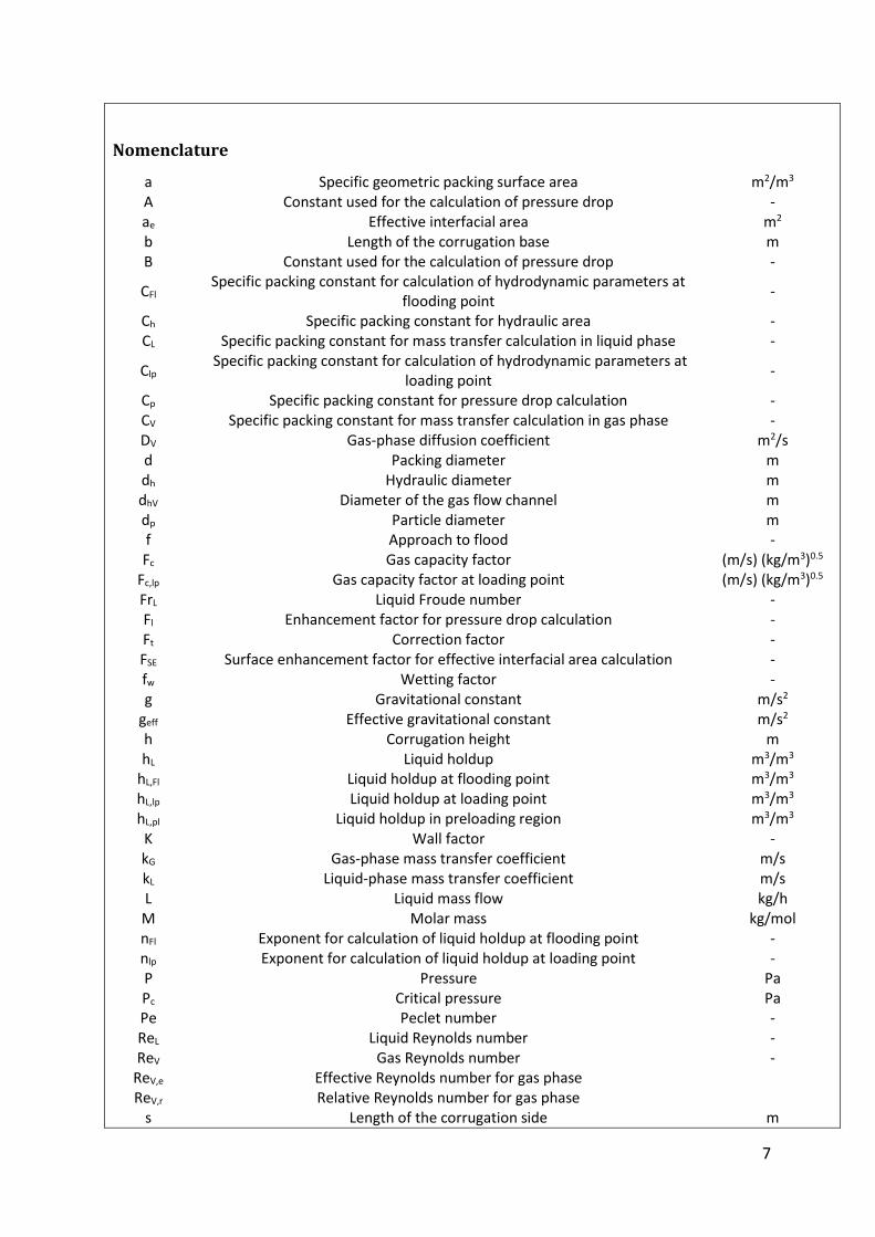
Nomenclature
a Specific geometric packing surface area m2/m3 A Constant used for the calculation of pressure drop - ae Effective interfacial area m2 b Length of the corrugation base m B Constant used for the calculation of pressure drop -
CFl Specific packing constant for calculation of hydrodynamic parameters at
flooding point -
Ch Specific packing constant for hydraulic area - CL Specific packing constant for mass transfer calculation in liquid phase -
Clp Specific packing constant for calculation of hydrodynamic parameters at
loading point -
Cp Specific packing constant for pressure drop calculation - CV Specific packing constant for mass transfer calculation in gas phase - DV Gas-phase diffusion coefficient m2/s d Packing diameter m dh Hydraulic diameter m dhV Diameter of the gas flow channel m dp Particle diameter m f Approach to flood - Fc Gas capacity factor (m/s) (kg/m3)0.5
Fc,lp Gas capacity factor at loading point (m/s) (kg/m3)0.5 FrL Liquid Froude number - Fl Enhancement factor for pressure drop calculation - Ft Correction factor - FSE Surface enhancement factor for effective interfacial area calculation - fw Wetting factor - g Gravitational constant m/s2
geff Effective gravitational constant m/s2 h Corrugation height m hL Liquid holdup m3/m3
hL,Fl Liquid holdup at flooding point m3/m3 hL,lp Liquid holdup at loading point m3/m3 hL,pl Liquid holdup in preloading region m3/m3 K Wall factor - kG Gas-phase mass transfer coefficient m/s kL Liquid-phase mass transfer coefficient m/s L Liquid mass flow kg/h M Molar mass kg/mol nFl Exponent for calculation of liquid holdup at flooding point - nlp Exponent for calculation of liquid holdup at loading point - P Pressure Pa Pc Critical pressure Pa Pe Peclet number - ReL Liquid Reynolds number - ReV Gas Reynolds number -
ReV,e Effective Reynolds number for gas phase ReV,r Relative Reynolds number for gas phase
s Length of the corrugation side m
8
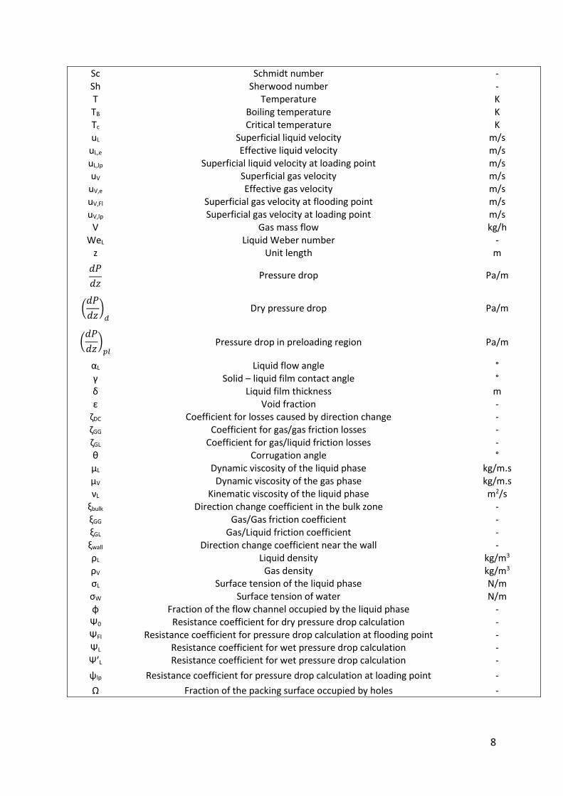
Sc Schmidt number - Sh Sherwood number - T Temperature K TB Boiling temperature K Tc Critical temperature K uL Superficial liquid velocity m/s
uL,e Effective liquid velocity m/s uL,lp Superficial liquid velocity at loading point m/s uV Superficial gas velocity m/s
uV,e Effective gas velocity m/s uV,Fl Superficial gas velocity at flooding point m/s uV,lp Superficial gas velocity at loading point m/s
V Gas mass flow kg/h WeL Liquid Weber number -
z Unit length m
𝑑𝑃
𝑑𝑧 Pressure drop Pa/m
(𝑑𝑃
𝑑𝑧)
𝑑 Dry pressure drop Pa/m
(𝑑𝑃
𝑑𝑧)
𝑝𝑙 Pressure drop in preloading region Pa/m
αL Liquid flow angle ° γ Solid – liquid film contact angle ° δ Liquid film thickness m ε Void fraction -
ζDC Coefficient for losses caused by direction change - ζGG Coefficient for gas/gas friction losses - ζGL Coefficient for gas/liquid friction losses - θ Corrugation angle ° µL Dynamic viscosity of the liquid phase kg/m.s µV Dynamic viscosity of the gas phase kg/m.s νL Kinematic viscosity of the liquid phase m2/s
ξbulk Direction change coefficient in the bulk zone - ξGG Gas/Gas friction coefficient - ξGL Gas/Liquid friction coefficient - ξwall Direction change coefficient near the wall - ρL Liquid density kg/m3 ρV Gas density kg/m3 σL Surface tension of the liquid phase N/m σW Surface tension of water N/m φ Fraction of the flow channel occupied by the liquid phase - Ψ0 Resistance coefficient for dry pressure drop calculation - ΨFl Resistance coefficient for pressure drop calculation at flooding point - ΨL Resistance coefficient for wet pressure drop calculation - Ψ’L Resistance coefficient for wet pressure drop calculation -
ψlp Resistance coefficient for pressure drop calculation at loading point -
Ω Fraction of the packing surface occupied by holes -
9
List of figures
Fig. 1: Distribution of final energy consumption in France [1] ................................................ 13
Fig. 2: Distribution of production of renewable energies by sector [1] ................................... 14
Fig. 3: Biogas primary production in 2013 [2] .......................................................................... 15
Fig. 4: Simplified diagram of production of biomethane ......................................................... 18
Fig. 5: Example of biogas utilization by Cryo Pur® Company [9].............................................. 20
Fig. 6: Vapor pressure of the main components present in biogas ......................................... 31
Fig. 7: Pressure – Temperature equilibrium behavior for the CH4 – CO2 system [29] ............. 32
Fig. 8: Pressure – Temperature equilibrium behavior for the CH4 – H2S system [30] ............. 33
Fig. 9: Biogas density as a function of temperature ................................................................ 34
Fig. 10: Biogas viscosity as a function of temperature ............................................................. 35
Fig. 11: Thermal conductivity of biogas as a function of temperature .................................... 36
Fig. 12: Heat capacity at constant pressure of biogas as a function of temperature .............. 37
Fig. 13: Heat capacity at constant volume of biogas as a function of temperature ................ 37
Fig. 14: Two-film theory [36] .................................................................................................... 41
Fig. 15: Chemical structure of some alkanolamines [43] ......................................................... 46
Fig. 16: Main gas-liquid contactors [48] ................................................................................... 49
Fig. 17: Schematic representation of a packed column ........................................................... 49
Fig. 18.a: Random packing Nutter Ring [Sulzer] ....................................................................... 50
Fig. 18.b : Structured packing Mellapak [Sulzer] ...................................................................... 50
Fig. 19: Transport mechanism of the adsorbate molecules on the adsorbent surface ........... 52
Fig. 20: Shapes of commercial activated carbons [53]............................................................. 53
Fig. 21: Effect of temperature on some adsorbents [57] ......................................................... 54
Fig. 22: Classification of adsorption isotherms [IUPAC] ........................................................... 56
Fig. 23: Skarstrom cycle stages and pressure variations [68] .................................................. 59
Fig. 24: Schematic representation of a membrane [71] .......................................................... 60
Fig. 25: Diagram of the main types of membranes [75] .......................................................... 62
Fig. 26: The geometric configurations of membrane contactors [76] ..................................... 63
Fig. 27: Most technologies used for the purification and upgrading of biogas [International Energy Agency] ......................................................................................................................... 66
Fig. 28: Comparison of investment costs of different biogas purification and upgrading technologies [88] ...................................................................................................................... 69
Fig. 29: BioGNVAL demonstrator located at Valenton water treatment plant [9] .................. 72
Fig. 30: Schematic representation of Cryo Pur® system [9] ..................................................... 73
Fig. 31: Simplified flowsheet of the BioGNVAL pilot plant [9] ................................................. 74
Fig. 32: Schematic diagram of the absorption subsystem for elimination of hydrogen sulfide [9] ............................................................................................................................................. 77
Fig. 33: Piping and instrumentation diagram of adsorption subsystem for the removal of hydrogen sulfide [9] ................................................................................................................ 78
Fig. 34: Carbon dioxide antisublimation [9] ............................................................................. 80
Fig. 35: Variation of the H2S content at the inlet and at the outlet of the absorption column .................................................................................................................................................. 81
Fig. 36: Variation of the biogas temperature at the inlet of the demonstrator and at the outlet of the absorption column .............................................................................................. 82
Fig. 37: Observation of the desorption phenomenon of H2S ................................................... 83
Fig. 38.a: Pressure drop evolution in a packing column .......................................................... 86
Fig. 38.b: Liquid holdup evolution in a packing column ........................................................... 86

10
Fig. 39.a. Pressure drop evaluation for liquid load uL = 20.5 m/h ........................................... 95
Fig. 39.b. Liquid holdup evaluation for liquid load uL = 20.5 m/h ............................................ 95
Fig. 40.a. Prediction of effective interfacial area by Billet and Schultes model for the system Air / Kerosol 200 ....................................................................................................................... 96
Fig. 40.b. Prediction of effective interfacial area by SRP model for the system Air / Kerosol 200 ............................................................................................................................................ 97
Fig. 40.c. Prediction of effective interfacial area by Delft model for the system Air / Kerosol 200 ............................................................................................................................................ 97
Fig. 41. Liquid holdup and pressure drop with an Air – Water system using Flexipac® 350Y packing ................................................................................................................................... 102
Fig. 42. Liquid holdup and pressure drop with an Air – Kerosol 200 system using Flexipac® 350Y packing ........................................................................................................................... 104
Fig. 43: Flowsheet of the absorption process simulated using Aspen Plus® ......................... 108
Fig. 44: Henry coefficients for CH4 – H2O system ................................................................... 110
Fig. 45: Henry coefficients for CO2 – H2O system ................................................................... 111
Fig. 46: Henry coefficients for H2S – H2O system ................................................................... 111
Fig. 47: Comparison between model and experimental data for heat capacity for carbon dioxide .................................................................................................................................... 112
Fig. 48: Deviation between experimental and calculated results of carbon dioxide heat capacity................................................................................................................................... 113
Fig. 49: Comparison between model and experimental data for liquid density of NaOH – H2O ................................................................................................................................................ 113
Fig. 50: Deviation between experimental and calculated results of liquid density ............... 114
Fig. 51: Comparison between model and experimental data for liquid viscosity of NaOH – H2O ......................................................................................................................................... 116
Fig. 52: Deviation between experimental and calculated results of liquid viscosity ............. 116
Fig. 53: Comparison between model and experimental data for liquid phase surface tension of 5 wt% NaOH aqueous solution .......................................................................................... 117
Fig. 54: Deviation between experimental and calculated results of surface tension ............ 118
Fig. 55: Comparison of results of equilibrium constant for reaction R.18 ............................. 120
Fig. 56: Comparison of results of reaction rate constant for reaction R.24 .......................... 121
Fig. 57: Deviation between experimental and calculated results of reaction rate constant (R.24) ...................................................................................................................................... 121
Fig. 58: Influence of the liquid flow on the absorption of hydrogen sulfide ......................... 123
Fig. 59: Influence of gas flow rate on the pressure drop ....................................................... 124
Fig. 60: Deviation between experimental and calculated results of pressure drop .............. 124
Fig. 61: Influence of the concentration of NaOH in the removal of H2S and CO2 .................. 125
Fig. 62: Influence of the temperature of liquid in the absorption of hydrogen sulfide ......... 126
Fig. 63: Deviation between experimental and calculated results of H2S concentration leaving the packing column ................................................................................................................ 126
Fig. 64: Influence of relative humidity in the adsorption of hydrogen sulfide using Airpel Ultra DS [53] .................................................................................................................................... 130
Fig. 65: Schematic representation of an adsorption column [122] ....................................... 131
Fig. 66: Influence of Langmuir equilibrium parameters on adsoption sites occupied .......... 137
Fig. 67: Breakthrough curve simulated for H2S molar percentage of 5 % ............................. 141
Fig. 68: Breakthrough curve simulated for H2S molar percentage of 7.5 % .......................... 141
Fig. 69: Breakthrough curve simulated for H2S molar percentage of 10 % ........................... 142

11
List of tables
Table 1. Concentration requirements before biogas liquefaction [8] ..................................... 19
Table 2. Composition and characterization of household waste [13] ..................................... 21
Table 3. Production yields for agricultural and agro-industrial substrates [14] ...................... 22
Table 4. Biogas composition depending on the type of substrate [14] ................................... 23
Table 5. Tolerances in impurities for the use of liquid biomethane as vehicle fuel [14] ......... 24
Table 6. Thermo-physical properties of hydrogen sulfide [19] ................................................ 28
Table 7. Thermo-physical properties of carbon dioxide [19] ................................................... 29
Table 8. Thermo-physical properties of methane [19] ............................................................ 30
Table 9. Constants used by Antoine Equation for the calculation of H2S, CO2 and CH4 vapor pressures .................................................................................................................................. 31
Table 10. Solubility of the main compounds of biogas in water [39] ...................................... 42
Table 11. Properties of physical solvents [40] ......................................................................... 43
Table 12. Solubility of gases in physical solvents at 25 °C and 0.1 MPa [41] ........................... 44
Table 13. Physical properties of some chemical solvents [43] ................................................ 45
Table 14. Classification of main gas-liquid contactors [48]...................................................... 48
Table 15. Criteria to differentiate between physical and chemical adsorption [49] ............... 51
Table 16. Equations governing adsorption isotherm models, and their linear forms [67] ..... 57
Table 17. The membrane materials used by manufacturer [71] ............................................. 60
Table 18. Classification of membrane separation processes [73] ........................................... 61
Table 19. Distribution of membranes according to pore size [IUPAC] .................................... 62
Table 20. Characteristics of the different geometries of membranes [76] ............................. 64
Table 21. Condensation or solidification temperatures, at atmospheric pressure, for the different compounds present in biogas ................................................................................... 65
Table 22. Effect of temperature on the abatement of volatile organic silicon compounds.... 65
Table 23. Comparison of the different biogas purification and upgrading technologies ........ 67
Table 24. Performances, costs, advantages and disadvantages of separation processes [87] 68
Table 25. Conditions and composition of the raw biogas treated by BioGNVAL pilot plant ... 75
Table 26. conditions of passage from one subsystem to another [9] ..................................... 75
Table 27. Sensitivities of measurement tools .......................................................................... 81
Table 28. Constants for the Billet and Schultes model [98] ..................................................... 87
Table 29. Effective interfacial area in packing columns using Billet and Schultes model [98] 87
Table 30. Liquid holdup and velocities at loading and flooding point [99] .............................. 88
Table 31. Liquid holdup in preloading and loading regions [98] .............................................. 89
Table 32. Pressure drop in packing columns using Billet and Schultes model [98] ................. 89
Table 33. Effective interfacial area in packing columns using SRP model [96] ........................ 90
Table 34. Liquid holdup in packing columns using SRP model [101] ....................................... 91
Table 35. Pressure drop in packing columns using SRP model [96] ......................................... 91
Table 36. Pressure drop in preloading region using Delft model [97] ..................................... 93
Table 37. Physical properties of the systems tested [100] ...................................................... 94
Table 38. Dimensions of Flexipac® 350Y [100] ......................................................................... 94
Table 39. Deviation between predictive models and experimental data ................................ 96
Table 40. Changes made to calculate liquid holdup ................................................................ 99
Table 41. Changes made to calculate Pressure drop for liquid density less than 900 kg.m-3 . 99
Table 42. Changes made to calculate Pressure drop for liquid density higher than 900 kg.m-3
................................................................................................................................................ 100
12
Table 43. Statistical deviation between the modified model and experimental data for pressure drop and liquid holdup predictions ......................................................................... 104
Table 44. Comparison between modified correlations and experimental data for the prediction of pressure drop in a structured packing column ................................................ 105
Table 45. Coefficients used by Aspen Plus® to calculate Henry’s constant ........................... 109
Table 46. Coefficients used by Harvey to calculate Henry’s constants .................................. 110
Table 47. Values of the constants used by Equation (87) to calculate the heat capacity of carbon dioxide ........................................................................................................................ 112
Table 48. Coefficients used in the calculation of the equilibrium constant .......................... 119
Table 49. Coefficients used in the calculation of the equilibrium constant of Reaction (R.6) ................................................................................................................................................ 119
Table 50. Parameters k and E for kinetic-controlled reactions [119] .................................... 120
Table 51. Details of the simulated process ............................................................................ 122
Table 52. Influence of liquid flow rate on the pressure drop ................................................ 123
Table 53. Activated carbon properties used for this study [53] ............................................ 129
Table 54. Biogas composition and operating conditions of the adsorption process ............. 132
Table 55. Sherwood number estimation [123] ...................................................................... 133
Table 56. Estimation of the binary diffusion coefficients [135] ............................................. 134
Table 57. Equations used to estimate internal diffusion coefficients ................................... 135
Table 58. Estimation of dimensionless numbers and diffusion coefficients ......................... 135
Table 59. Boundary and initial conditions of the system ....................................................... 138
Table 60. Input parameters for the simulation of the breakthrough curve .......................... 140
13
General introduction
Recent decades were accompanied by economic growth and prosperity for humanity. This growth gained from oil and natural gas production has been accompanied by an environmental pollution that may trigger irreversible changes in the environment with catastrophic consequences for humans. Moreover, issues related to the reduction of fossil reserves are still relevant, and the global primary energy demand is increasing, pushing the international community to pursue the development of renewable energies.
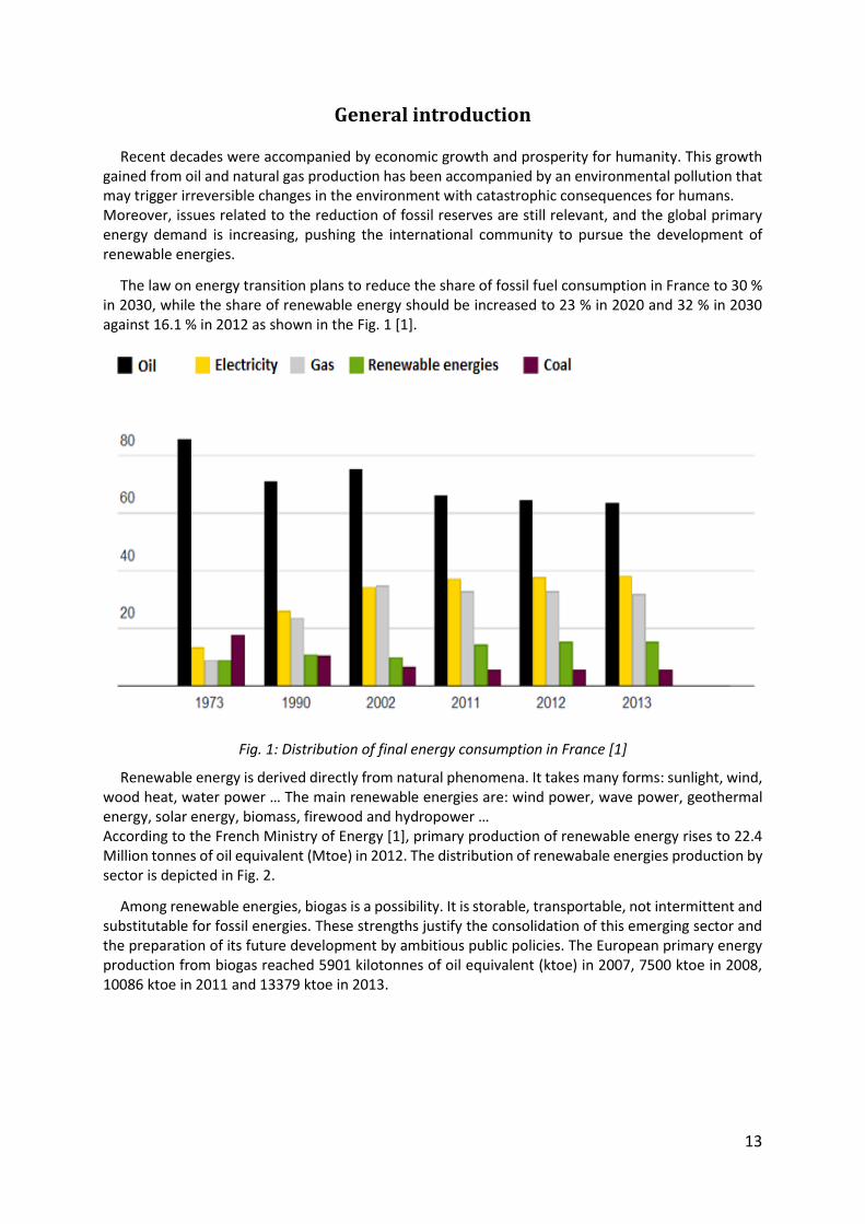
The law on energy transition plans to reduce the share of fossil fuel consumption in France to 30 % in 2030, while the share of renewable energy should be increased to 23 % in 2020 and 32 % in 2030 against 16.1 % in 2012 as shown in the Fig. 1 [1].
Fig. 1: Distribution of final energy consumption in France [1]
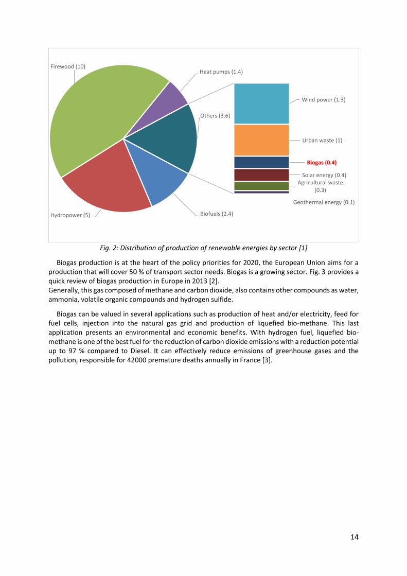
Renewable energy is derived directly from natural phenomena. It takes many forms: sunlight, wind, wood heat, water power … The main renewable energies are: wind power, wave power, geothermal energy, solar energy, biomass, firewood and hydropower … According to the French Ministry of Energy [1], primary production of renewable energy rises to 22.4 Million tonnes of oil equivalent (Mtoe) in 2012. The distribution of renewabale energies production by sector is depicted in Fig. 2.
Among renewable energies, biogas is a possibility. It is storable, transportable, not intermittent and substitutable for fossil energies. These strengths justify the consolidation of this emerging sector and the preparation of its future development by ambitious public policies. The European primary energy production from biogas reached 5901 kilotonnes of oil equivalent (ktoe) in 2007, 7500 ktoe in 2008, 10086 ktoe in 2011 and 13379 ktoe in 2013.
14
Fig. 2: Distribution of production of renewable energies by sector [1]
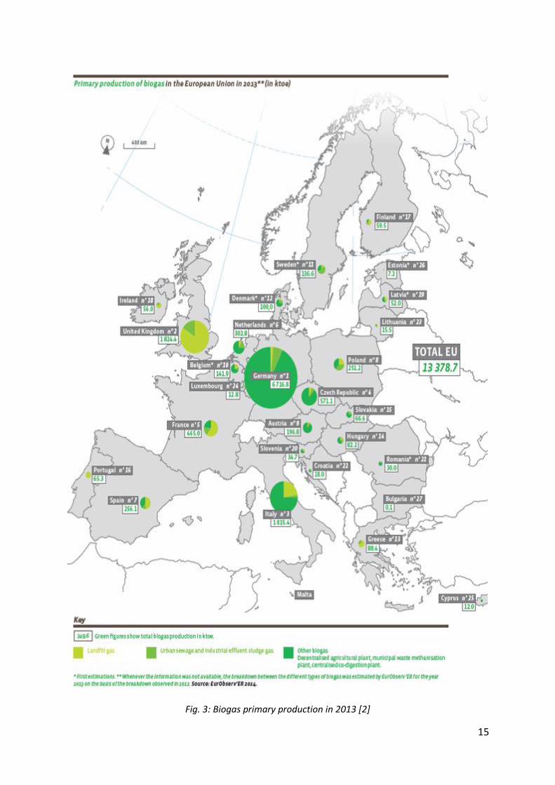
Biogas production is at the heart of the policy priorities for 2020, the European Union aims for a production that will cover 50 % of transport sector needs. Biogas is a growing sector. Fig. 3 provides a quick review of biogas production in Europe in 2013 [2]. Generally, this gas composed of methane and carbon dioxide, also contains other compounds as water, ammonia, volatile organic compounds and hydrogen sulfide.
Biogas can be valued in several applications such as production of heat and/or electricity, feed for fuel cells, injection into the natural gas grid and production of liquefied bio-methane. This last application presents an environmental and economic benefits. With hydrogen fuel, liquefied bio-methane is one of the best fuel for the reduction of carbon dioxide emissions with a reduction potential up to 97 % compared to Diesel. It can effectively reduce emissions of greenhouse gases and the pollution, responsible for 42000 premature deaths annually in France [3].
Biofuels (2.4)Hydropower (5)
Firewood (10)Heat pumps (1.4)
Wind power (1.3)
Urban waste (1)
Biogas (0.4)
Solar energy (0.4)Agricultural waste
(0.3)
Geothermal energy (0.1)
Others (3.6)
15
Fig. 3: Biogas primary production in 2013 [2]
16
Liquefied bio-methane requires very low temperatures which may lead to solidification of impurities and thus facilities malfunctions. These impurities must be separated from the biogas. This implies implementation of a purification process to remove from the raw biogas all unwanted substances in order to maximize its methane content. In particular, the complete desulfurization of biogas is peremptory in order to ensure an optimal operation and a high purity of other compounds to valorize, such as carbon dioxide. Moreover, the presence of hydrogen sulfide in the wet biogas, is a poison for installations. In case of leakage, the presence of hydrogen sulphide in the biogas characterized by a rotten egg smell can be dangerous for operators working on the site. Hence, the need to remove all traces of this compound. Several technologies are used for the removal of H2S as adsorption on microporous solids, membrane technology, biological processes and absorption by means of liquid solvents.
The choice of the technique to implement is related to various parameters. The most important are the flow rate of biogas and hydrogen sulfide concentrations to treat. The solution must also respond to various economic, environmental and energetic imperatives as cost which must be reasonable, the threshold to reject which must be respected in an energy-efficient process. Therefore, there is no universal treatment method.
In this thesis, the choice fell on the use of a cryogenic method in order to combine biogas upgrading and biomethane liquefaction. The removal of H2S will be performed upstream of the process either by reactive absorption using an aqueous solution of sodium hydroxide (NaOH) in a structured packed column or by adsorption using activated carbon. These two technologies will be tested and compared in order to choose the most effective and the most suitable for the process set up.
Experiments were performed on a industrial pilot plant developed by Cryo Pur® company called “BioGNVAL”. This pilot plant treats 85 Nm3/h of biogas from waste water treatment plant, which contains around 20 – 100 ppm of H2S.
For absorption technology, the hydrodynamic of flows in structured packing columns was studied in order to develop a model able to predict realistically the key hydrodynamic parameters as pressure drop, liquid holdup and transition points but also effective interfacial area and global mass transfer coefficients.
The remainder of the study is based on simulations using Aspen Plus® V8.0 to study realistically the effectiveness of a structured packed column which uses sodium hydroxide as a chemical solvent for the selective removal of hydrogen sulfide from biogas. Results were compared with data from BioGNVAL pilot plant.
Finally, the dynamic aspect of the adsorption phenomenon is modeled, by predicting the breakthrough curve in the case of an adsorption column used for the removal of H2S.

17
Chapter 1: From biogas to biomethane Résumé :
Après une introduction générale posant le contexte de la production de biogaz dans le paysage énergétique mondial, le premier chapitre est une introduction à la problématique de son obtention et de son usage sous une version raffinée en biométhane.
Le biogaz est produit par méthanisation lorsque des matières organiques sont décomposées dans des conditions bien définies et en absence d’oxygène. Il est constitué principalement de méthane et de dioxyde de carbone mais aussi de quantités variables de vapeur d’eau, de sulfure d’hydrogène et d’autres composés polluants. Afin de pouvoir utiliser le biogaz comme carburant pour véhicule, il doit être épuré en séparant le dioxyde de carbone et les autres composés contaminants du biogaz pour augmenter au maximum sa teneur en méthane.
Il existe différentes technologies utilisées dans le domaine du traitement des gaz. Les plus utilisées sont : l’absorption, l’adsorption, la technologie membranaire, la cryogénie, le traitement biologique et l’oxydation. Aujourd'hui, d'autres technologies sont développées telles que la biocatalyse, la photocatalyse et le plasma froid. Pour le moment, le manque d'informations à leur sujet limite leur application industrielle [18].
18
1.1. Introduction
Anaerobic digestion may be defined as the natural process of degradation by microorganisms under controlled conditions and in the absence of oxygen. This degradation results in the production of a gas mixture saturated with water outlet of the digester called biogas.
Anaerobic digestion is the result of four biochemical steps in which large carbon chains are converted into fatty acids and alcohols. These four steps are: Hydrolysis, acidogenesis, acetogenesis, methanogenesis [4].
Hydrolysis
It takes place at the beginning of the fermentation and makes use of exo-enzymes in order to decompose the organic matter into simple substances.
Acidogenesis
During this step, volatile fatty acids are formed. Carbon dioxide and hydrogen are also formed, they are used by microorganisms during the production of methane according to the chemical Reaction (R.1) shown below. The reaction enthalpy is about -567 kJ.mol-1 [5].
𝐶𝑂2 + 4 𝐻2 → 𝐶𝐻4 + 2 𝐻2𝑂 (R.1)
Acetogenesis
This stage involves the production of acetate, an indispensable substrate for the synthesis of methane.
Methanogenesis
This last step results in the production of methane. It is ensured by the methanogenic bacteria, which can only use a limited number of carbon compounds, including acetate responsible for 70 % of methane production according to the chemical Reaction (R.2) shown below. The reaction enthalpy is about -130 kJ.mol-1 [5].
𝐶𝐻3𝐶𝑂𝑂𝐻 + 𝐻2𝑂 → 𝐶𝐻4 + 𝐻2𝐶𝑂3 (R.2)
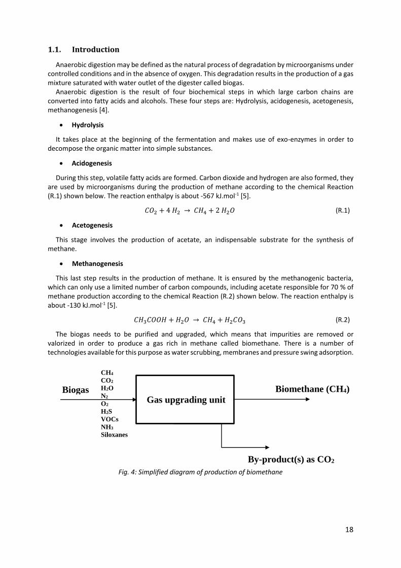
The biogas needs to be purified and upgraded, which means that impurities are removed or valorized in order to produce a gas rich in methane called biomethane. There is a number of technologies available for this purpose as water scrubbing, membranes and pressure swing adsorption.
Fig. 4: Simplified diagram of production of biomethane
Gas upgrading unit
Biogas Biomethane (CH4)
By-product(s) as CO2
CH4
CO2
H2O
N2
O2
H2S
VOCs
NH3
Siloxanes
19
1.2. Biogas utilization
Biogas can be used in several applications. Sometimes it could be used raw, but almost always it has to be upgraded or as a minimum cleaned from its H2S content because the presence of this compound in the biogas even at very low concentrations could damage the installations.
Biogas can be used in all applications designed for natural gas such us production of heat and electricity known as combined heat and power (CHP), production of chemicals and/or proteins, fueling internal combustion engines and fuel cells, it may also be used as vehicle fuel or injected in the natural gas grids.
1.2.1. Direct combustion
The simplest method of biogas utilization is direct combustion. The biogas burner can be installed in heaters for production of hot water and hot air, in dryers for various materials, and in boilers for production of steam for process heat or power generation [6]. Another limited application involves absorption heating and cooling to provide chilled water for refrigeration and hot water for industrial processes. These applications based on direct combustion do not require a high gas quality.
Biogas can also be used to fuel internal combustion engines to supply electric power for pumps, blowers, elevator and conveyors, heat pumps and air conditioners [7].
1.2.2. Combined heat and power
Another application for biogas is CHP which involves the production of two or more forms of energy, generally electricity and thermal energy. This latter is generally the most used today but it could be a problem because the need of heat varies with season, and during summer for example, unused biogas is flared.
1.2.3. Injection into the natural gas grid
Upgrading of biogas to biomethane with a gas quality similar to natural gas and injecting it into the natural gas grid is an efficient way to integrate biogas into the energy sector. It allows the transport of large volume of biomethane and its utilization in wide areas where population is concentrated.
1.2.4. Vehicle fuel
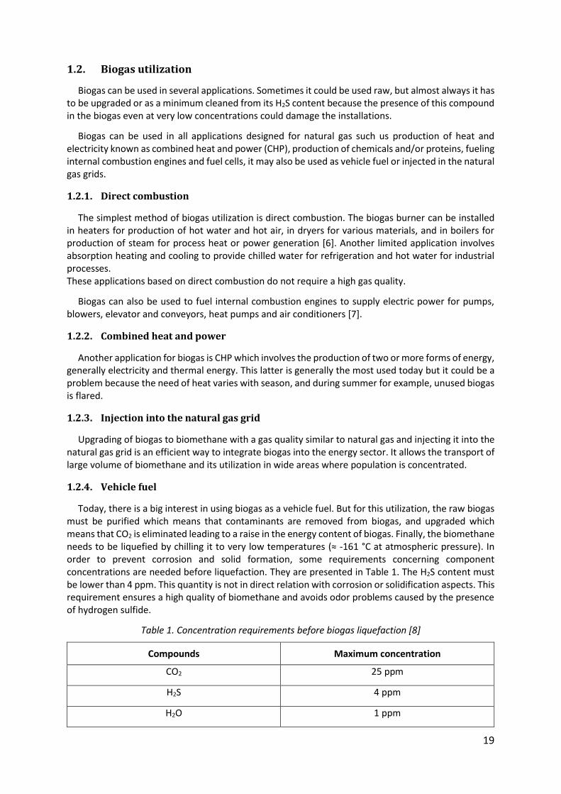
Today, there is a big interest in using biogas as a vehicle fuel. But for this utilization, the raw biogas must be purified which means that contaminants are removed from biogas, and upgraded which means that CO2 is eliminated leading to a raise in the energy content of biogas. Finally, the biomethane needs to be liquefied by chilling it to very low temperatures (≈ -161 °C at atmospheric pressure). In order to prevent corrosion and solid formation, some requirements concerning component concentrations are needed before liquefaction. They are presented in Table 1. The H2S content must be lower than 4 ppm. This quantity is not in direct relation with corrosion or solidification aspects. This requirement ensures a high quality of biomethane and avoids odor problems caused by the presence of hydrogen sulfide.
Table 1. Concentration requirements before biogas liquefaction [8]
Compounds Maximum concentration
CO2 25 ppm
H2S 4 ppm
H2O 1 ppm
20
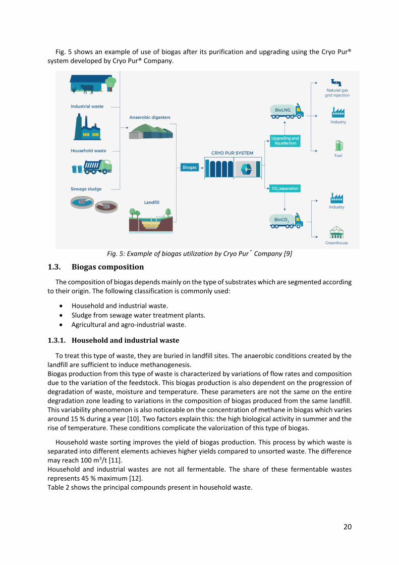
Fig. 5 shows an example of use of biogas after its purification and upgrading using the Cryo Pur® system developed by Cryo Pur® Company.
Fig. 5: Example of biogas utilization by Cryo Pur® Company [9]
1.3. Biogas composition
The composition of biogas depends mainly on the type of substrates which are segmented according to their origin. The following classification is commonly used:
Household and industrial waste.
Sludge from sewage water treatment plants.
Agricultural and agro-industrial waste.
1.3.1. Household and industrial waste
To treat this type of waste, they are buried in landfill sites. The anaerobic conditions created by the landfill are sufficient to induce methanogenesis. Biogas production from this type of waste is characterized by variations of flow rates and composition due to the variation of the feedstock. This biogas production is also dependent on the progression of degradation of waste, moisture and temperature. These parameters are not the same on the entire degradation zone leading to variations in the composition of biogas produced from the same landfill. This variability phenomenon is also noticeable on the concentration of methane in biogas which varies around 15 % during a year [10]. Two factors explain this: the high biological activity in summer and the rise of temperature. These conditions complicate the valorization of this type of biogas.
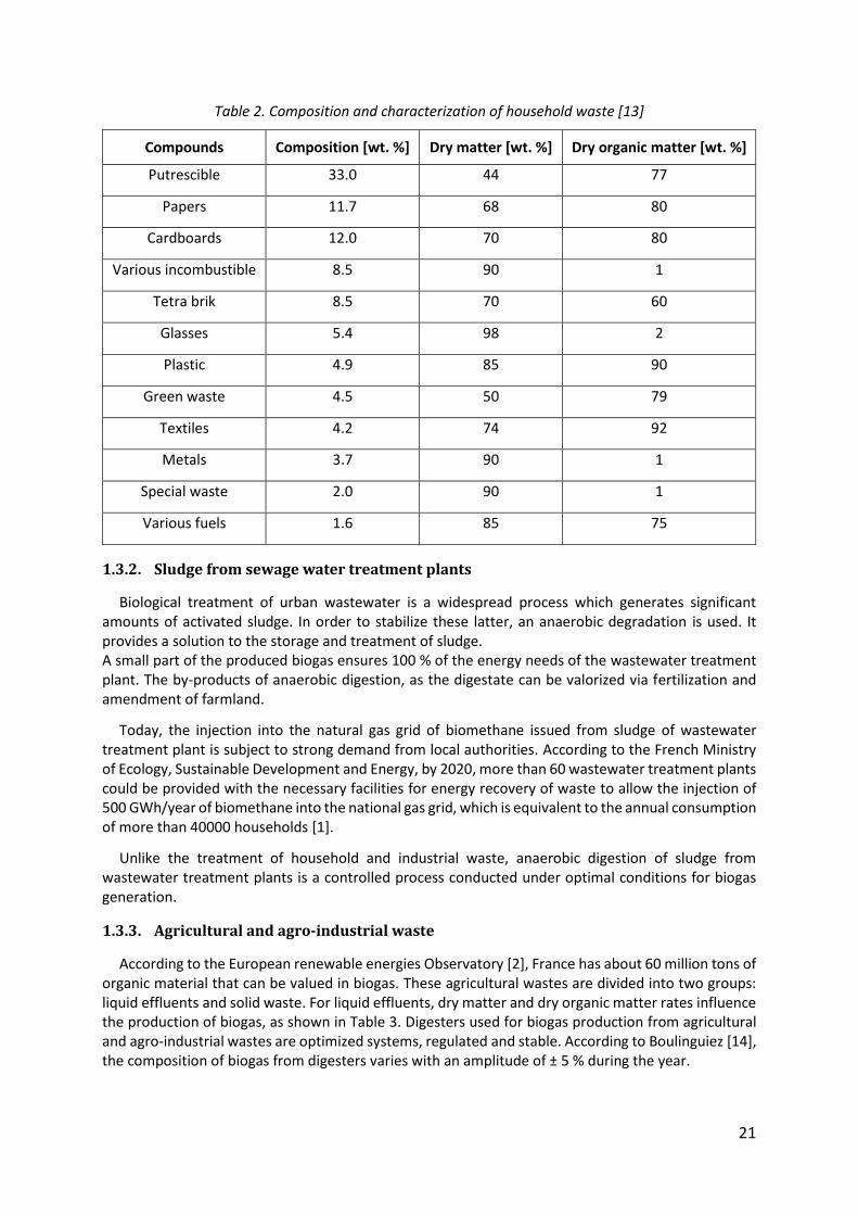
Household waste sorting improves the yield of biogas production. This process by which waste is separated into different elements achieves higher yields compared to unsorted waste. The difference may reach 100 m3/t [11]. Household and industrial wastes are not all fermentable. The share of these fermentable wastes represents 45 % maximum [12]. Table 2 shows the principal compounds present in household waste.
21
Table 2. Composition and characterization of household waste [13]
Compounds Composition [wt. %] Dry matter [wt. %] Dry organic matter [wt. %]
Putrescible 33.0 44 77
Papers 11.7 68 80
Cardboards 12.0 70 80
Various incombustible 8.5 90 1
Tetra brik 8.5 70 60
Glasses 5.4 98 2
Plastic 4.9 85 90
Green waste 4.5 50 79
Textiles 4.2 74 92
Metals 3.7 90 1
Special waste 2.0 90 1
Various fuels 1.6 85 75
1.3.2. Sludge from sewage water treatment plants
Biological treatment of urban wastewater is a widespread process which generates significant amounts of activated sludge. In order to stabilize these latter, an anaerobic degradation is used. It provides a solution to the storage and treatment of sludge. A small part of the produced biogas ensures 100 % of the energy needs of the wastewater treatment plant. The by-products of anaerobic digestion, as the digestate can be valorized via fertilization and amendment of farmland.
Today, the injection into the natural gas grid of biomethane issued from sludge of wastewater treatment plant is subject to strong demand from local authorities. According to the French Ministry of Ecology, Sustainable Development and Energy, by 2020, more than 60 wastewater treatment plants could be provided with the necessary facilities for energy recovery of waste to allow the injection of 500 GWh/year of biomethane into the national gas grid, which is equivalent to the annual consumption of more than 40000 households [1].
Unlike the treatment of household and industrial waste, anaerobic digestion of sludge from wastewater treatment plants is a controlled process conducted under optimal conditions for biogas generation.
1.3.3. Agricultural and agro-industrial waste
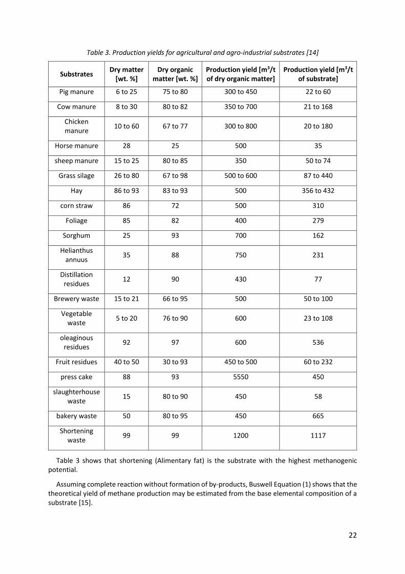
According to the European renewable energies Observatory [2], France has about 60 million tons of organic material that can be valued in biogas. These agricultural wastes are divided into two groups: liquid effluents and solid waste. For liquid effluents, dry matter and dry organic matter rates influence the production of biogas, as shown in Table 3. Digesters used for biogas production from agricultural and agro-industrial wastes are optimized systems, regulated and stable. According to Boulinguiez [14], the composition of biogas from digesters varies with an amplitude of ± 5 % during the year.
22
Table 3. Production yields for agricultural and agro-industrial substrates [14]
Substrates Dry matter
[wt. %] Dry organic
matter [wt. %] Production yield [m3/t of dry organic matter]
Production yield [m3/t of substrate]
Pig manure 6 to 25 75 to 80 300 to 450 22 to 60
Cow manure 8 to 30 80 to 82 350 to 700 21 to 168
Chicken manure
10 to 60 67 to 77 300 to 800 20 to 180
Horse manure 28 25 500 35
sheep manure 15 to 25 80 to 85 350 50 to 74
Grass silage 26 to 80 67 to 98 500 to 600 87 to 440
Hay 86 to 93 83 to 93 500 356 to 432
corn straw 86 72 500 310
Foliage 85 82 400 279
Sorghum 25 93 700 162
Helianthus annuus
35 88 750 231
Distillation residues
12 90 430 77
Brewery waste 15 to 21 66 to 95 500 50 to 100
Vegetable waste
5 to 20 76 to 90 600 23 to 108
oleaginous residues
92 97 600 536
Fruit residues 40 to 50 30 to 93 450 to 500 60 to 232
press cake 88 93 5550 450
slaughterhouse waste
15 80 to 90 450 58
bakery waste 50 80 to 95 450 665
Shortening waste
99 99 1200 1117
Table 3 shows that shortening (Alimentary fat) is the substrate with the highest methanogenic potential.
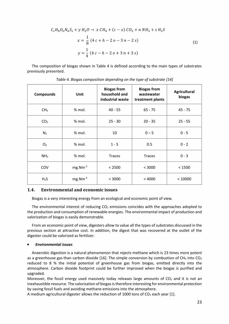
Assuming complete reaction without formation of by-products, Buswell Equation (1) shows that the theoretical yield of methane production may be estimated from the base elemental composition of a substrate [15].
23
𝐶𝑐𝐻ℎ𝑂𝑜𝑁𝑛𝑆𝑠 + 𝑦 𝐻2𝑂 → 𝑥 𝐶𝐻4 + (𝑐 − 𝑥) 𝐶𝑂2 + 𝑛 𝑁𝐻3 + 𝑠 𝐻2𝑆
𝑥 = 1
8 (4 𝑐 + ℎ − 2 𝑜 − 3 𝑛 − 2 𝑠)
𝑦 =1
4 (4 𝑐 − ℎ − 2 𝑜 + 3 𝑛 + 3 𝑠)
(1)
The composition of biogas shown in Table 4 is defined according to the main types of substrates previously presented.
Table 4. Biogas composition depending on the type of substrate [14]
Compounds Unit Biogas from
household and industrial waste
Biogas from wastewater
treatment plants
Agricultural biogas
CH4 % mol. 40 - 55 65 - 75 45 - 75
CO2 % mol. 25 - 30 20 - 35 25 - 55
N2 % mol. 10 0 – 5 0 - 5
O2 % mol. 1 - 5 0.5 0 - 2
NH3 % mol. Traces Traces 0 - 3
COV mg.Nm-3 < 2500 < 3000 < 1500
H2S mg.Nm-3 < 3000 < 4000 < 10000
1.4. Environmental and economic issues
Biogas is a very interesting energy from an ecological and economic point of view.
The environmental interest of reducing CO2 emissions coincides with the approaches adopted to the production and consumption of renewable energies. The environmental impact of production and valorization of biogas is easily demonstrable.
From an economic point of view, digesters allow to value all the types of substrates discussed in the previous section at attractive cost. In addition, the digest that was recovered at the outlet of the digester could be valorized as fertilizer.
Environmental issues
Anaerobic digestion is a natural phenomenon that rejects methane which is 23 times more potent as a greenhouse gas than carbon dioxide [16]. The simple conversion by combustion of CH4 into CO2 reduced to 8 % the initial potential of greenhouse gas from biogas, emitted directly into the atmosphere. Carbon dioxide footprint could be further improved when the biogas is purified and upgraded. Moreover, the fossil energy used massively today releases large amounts of CO2 and it is not an inexhaustible resource. The valorization of biogas is therefore interesting for environmental protection by saving fossil fuels and avoiding methane emissions into the atmosphere. A medium agricultural digester allows the reduction of 1000 tons of CO2 each year [1].
24
Economic issues
The economic feasibility of a biogas sector depends mainly on the composition of the biogas.
The methane concentration in a biogas produced from household and industrial wastes is low as seen in Table 4. The CH4 concentrations do not exceed 55 %. Moreover, the biogas produced can vary over time and it contains large amount of minor compounds, complicating biogas valorization. Biogas production from this type of waste is expected to be limited in future years in Europe. Restrictions and European standards are becoming more stringent, which makes the use of this source, unprofitable [12]. The most advanced biogas applications as vehicle fuel production or injection into the natural gas grid are hardly possible from this source, which requires advanced purification treatments. Considering an anaerobic digestion unit treating 50000 t/year of household waste, the total costs vary between 50 and 95 €/t while the incomes do not exceed 30 €/t [14].
The economic balance of biogas production within wastewater treatment plants depends on the size and savings made on the sludge. This stable and controlled anaerobic digestion process is financially viable. The wastewater treatment plant “Aquapol” situated in Grenoble, France treats 88 000 000 m3 of wastewater each year which is equivalent to 8000 dry tons of sludge processed per year. Part of the produced biogas is used for internal energy needs of the plant (8 GWh/year). The other part (14 GWh/year) will be injected in the natural gas grid after purification and compression [17].
The establishment of biogas purification process from agricultural waste is particularly attractive due to the reliability of the resource. The introduction of energy crops among the substrates improves the performance of anaerobic digestion giving a new economic aspect for the production of biogas.
1.5. From biogas to liquid biomethane
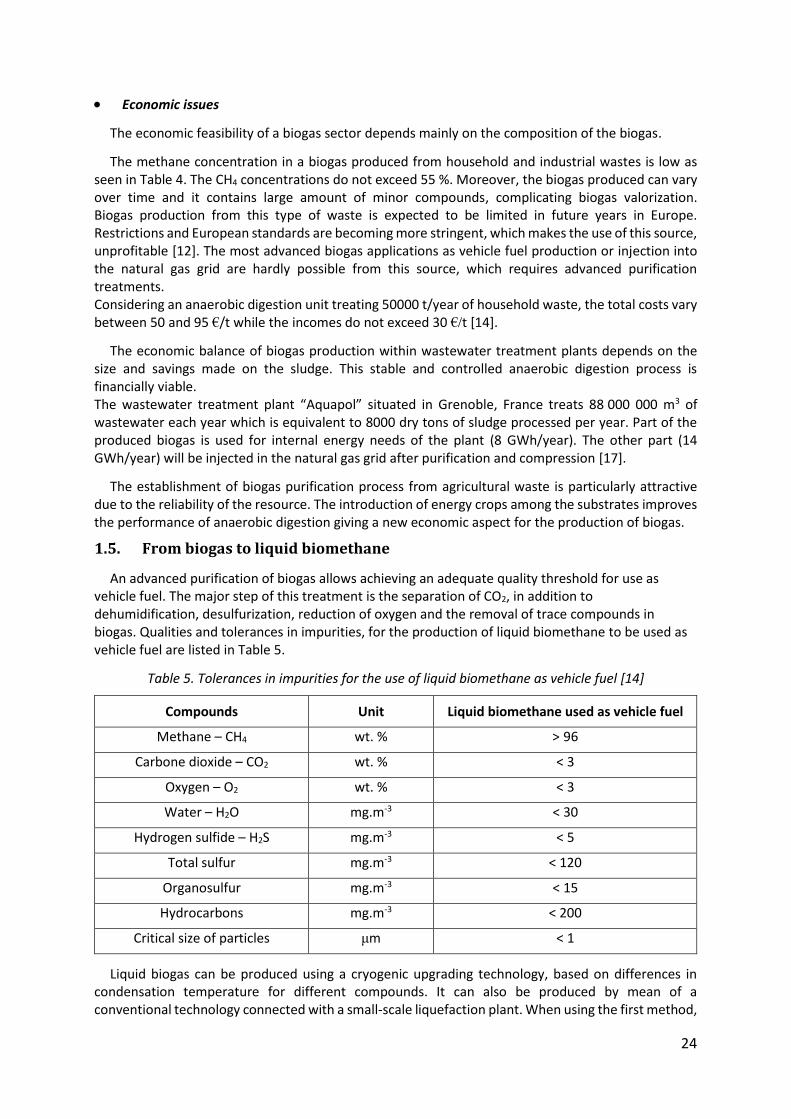
An advanced purification of biogas allows achieving an adequate quality threshold for use as vehicle fuel. The major step of this treatment is the separation of CO2, in addition to dehumidification, desulfurization, reduction of oxygen and the removal of trace compounds in biogas. Qualities and tolerances in impurities, for the production of liquid biomethane to be used as vehicle fuel are listed in Table 5.
Table 5. Tolerances in impurities for the use of liquid biomethane as vehicle fuel [14]
Compounds Unit Liquid biomethane used as vehicle fuel
Methane – CH4 wt. % > 96
Carbone dioxide – CO2 wt. % < 3
Oxygen – O2 wt. % < 3
Water – H2O mg.m-3 < 30
Hydrogen sulfide – H2S mg.m-3 < 5
Total sulfur mg.m-3 < 120
Organosulfur mg.m-3 < 15
Hydrocarbons mg.m-3 < 200
Critical size of particles μm < 1
Liquid biogas can be produced using a cryogenic upgrading technology, based on differences in condensation temperature for different compounds. It can also be produced by mean of a conventional technology connected with a small-scale liquefaction plant. When using the first method,
25
the carbon dioxide comes as a by-product which could be used in external applications bringing in extra income to the biogas upgrading unit.
The environmental benefits provided by the passage from the diesel to biomethane are impressive. Used as a fuel, Bio-LNG enables a considerable reduction of polluting emissions and represents a genuine alternative to diesel:
Zero emission of fine particles responsible for 42000 premature deaths annually in France.
-70 % NOx emissions.
-90 % CO2 emissions.
-99 % hydrocarbons emissions.
-50 % noise pollution.
Bio-LNG is a renewable energy produced from waste which makes it neutral in terms of greenhouse gas emissions. Its use allows the decarbonization of the energy mix. Bio-LNG is the only sustainable solution for long-distance haulage operated by heavy goods vehicles.
1.6. Conclusion
Biogas is produced when organic material is decomposed under anaerobic conditions. The main constituents are methane and carbon dioxide. To be able to use the raw biogas as a vehicle fuel it must be purified and upgraded, which means that impurities and CO2 respectively, are separated. There are a number of available upgrading technologies and the most commonly used are:
Absorption
Adsorption
Membranes
Cryogenic technology
Other technologies exist such as oxidation and biological treatment. These techniques are known in the field of gas treatment. Today other technologies are being developed such as biocatalysis, photocatalysis and cold plasma. For the moment, the lack of information about them limits their industrial application [18].
The choice of the technology to be used to purify, upgrade and liquefy the biogas requires the knowledge of the thermodynamic properties of biogas and the representation of phase equilibrium. These thermodynamics aspects of biogas will be discussed in the next chapter.
26
Chapter 2: Thermodynamic aspects of biogas Résumé :
Le choix de la technologie à utiliser pour purifier et liquéfier le biogaz exige la connaissance des propriétés thermodynamiques du biogaz.
Ce chapitre recense les propriétés thermodynamiques des fluides qui sont essentielles pour concevoir et optimiser les technologies de purification de biogaz. Il montre aussi que les propriétés thermophysiques du biogaz dépendent fortement de sa composition, en particulier des concentrations de méthane et de dioxyde de carbone. La présence de composés à faibles concentrations comme l’azote ou l’hydrogène sulfuré pourrait modifier les propriétés physiques du biogaz. Par exemple, les gaz d'enfouissement comprennent de petites quantités d'azote et d'oxygène qui affectent le comportement de phase du système CH4 – CO2.
27
2.1. Introduction
Thermodynamics can be used as a powerful tool for setting and evaluating processes used for purification and upgrading of biogas. Therefore, this study will focus on the thermodynamic investigation of biogas. It will present the thermodynamic properties of pure compounds and of the gas mixture (biogas) at a pressure of 1.103 bar. This pressure is considered because the biogas treated in the experimental part (Chapter 4) comes from the wastewater treatment plant at a pressure slightly above atmospheric pressure in order to avoid air infiltration into the biogas pipe.
2.2. Thermodynamic properties of pure component present in biogas
Biogas refers to a mixture of different molecules of gases as seen in Table 4. The thermodynamic aspects of the main components of biogas will be presented in this section.
2.2.1. Hydrogen sulfide
Hydrogen sulfide is a colorless gas with the characteristic foul odor of rotten eggs. It is very poisonous, corrosive, flammable and explosive. Its olfactory threshold varies between 0.7 and 200 g.m-
3, depending on the sensitivity of each individual. The olfactory sensation is not proportional to the concentration of H2S in the air because it is possible that the smell felt at very low concentrations is attenuated or disappeared at high concentrations.
Hydrogen sulfide is created following the bacterial decomposition of organic matter in the absence of oxygen, such as in swamps and sewers. It also appears in volcanic gases and hot springs. Other sources of hydrogen sulfide are the industrial processes used in the oil and natural gas sectors, sewage treatment plants and factories producing pulp and paper … The thermos-physical properties of hydrogen sulfide are listed in Table 6.

28
Table 6. Thermo-physical properties of hydrogen sulfide [19]
Properties Unit Value
Molar mass g.mol-1 34.08
Auto-ignition temperature °C 270
Solubility in water (1.013 bar and 0 °C)
vol/vol 4.67
Solid phase
Melting point °C -85.7
Latent heat of fusion (1.013 bar at melting point)
kJ.kg-1 69.73
Liquid phase
Boiling point at 1.013 bar °C -60.3
Vapor pressure at 20 °C bar 17.81
Liquid phase density (1.013 bar at boiling point)
kg.m-3 949.2
Latent heat of vaporization (1.013 bar at boiling point)
kJ.kg-1 546.41
Gas phase
Gas phase density (1.013 bar and 15 °C)
kg.m-3 1.45
Viscosity (1.013 bar and 0 °C) Pa.s 1.13 x 10⁻⁵
Thermal conductivity (1.013 bar and 0 °C)
mW.m-1.K-1 15.61
Specific volume (1.013 bar and 25 °C)
m3.kg-1 0.7126
Heat capacity at constant pressure (1.013 bar and 25 °C)
kJ.mol-1.K-1 0.0346
Heat capacity at constant volume (1.013 bar and 25 °C)
kJ.mol-1.K-1 0.026
Critical point
Critical temperature °C 99.95
Critical pressure bar 90
Critical density kg.m-3 347.28
Triple point
Triple point temperature °C -85.45
Triple point pressure bar 0.232
2.2.2. Carbon dioxide
Carbon dioxide is a colorless and odorless gas which is naturally present in the Earth's atmosphere. The concentration of carbon dioxide in the atmosphere reached 405 ppm at the end of 2016, against only 283 ppm in 1839.
Carbon dioxide is produced by all aerobic organisms when they metabolize carbohydrate and lipids to produce energy by respiration [20]. It is also produced by burning fossil fuels such as coal, natural gas and oil. Significant amounts of CO2 are also released by volcanoes. The thermos-physical properties of carbon dioxide are listed in Table 7.
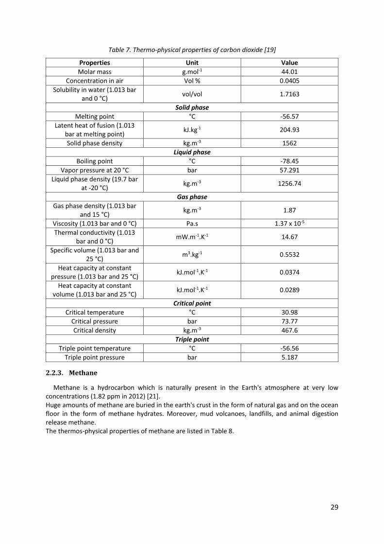
29
Table 7. Thermo-physical properties of carbon dioxide [19]
Properties Unit Value
Molar mass g.mol-1 44.01
Concentration in air Vol % 0.0405
Solubility in water (1.013 bar and 0 °C)
vol/vol 1.7163
Solid phase
Melting point °C -56.57
Latent heat of fusion (1.013 bar at melting point)
kJ.kg-1 204.93
Solid phase density kg.m-3 1562
Liquid phase
Boiling point °C -78.45
Vapor pressure at 20 °C bar 57.291
Liquid phase density (19.7 bar at -20 °C)
kg.m-3 1256.74
Gas phase
Gas phase density (1.013 bar and 15 °C)
kg.m-3 1.87
Viscosity (1.013 bar and 0 °C) Pa.s 1.37 x 10⁻⁵
Thermal conductivity (1.013 bar and 0 °C)
mW.m-1.K-1 14.67
Specific volume (1.013 bar and 25 °C)
m3.kg-1 0.5532
Heat capacity at constant pressure (1.013 bar and 25 °C)
kJ.mol-1.K-1 0.0374
Heat capacity at constant volume (1.013 bar and 25 °C)
kJ.mol-1.K-1 0.0289
Critical point
Critical temperature °C 30.98
Critical pressure bar 73.77
Critical density kg.m-3 467.6
Triple point
Triple point temperature °C -56.56
Triple point pressure bar 5.187
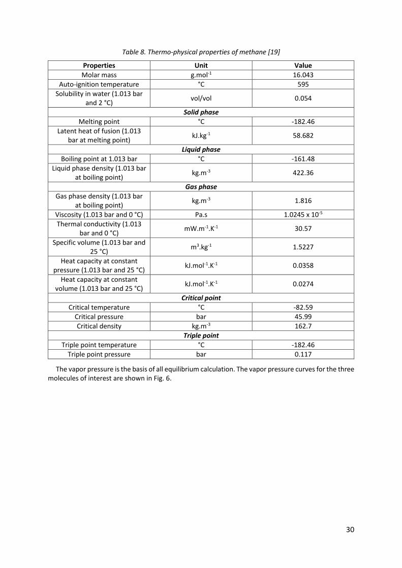
2.2.3. Methane
Methane is a hydrocarbon which is naturally present in the Earth's atmosphere at very low concentrations (1.82 ppm in 2012) [21]. Huge amounts of methane are buried in the earth's crust in the form of natural gas and on the ocean floor in the form of methane hydrates. Moreover, mud volcanoes, landfills, and animal digestion release methane. The thermos-physical properties of methane are listed in Table 8.
30
Table 8. Thermo-physical properties of methane [19]
Properties Unit Value
Molar mass g.mol-1 16.043
Auto-ignition temperature °C 595
Solubility in water (1.013 bar and 2 °C)
vol/vol 0.054
Solid phase
Melting point °C -182.46
Latent heat of fusion (1.013 bar at melting point)
kJ.kg-1 58.682
Liquid phase
Boiling point at 1.013 bar °C -161.48
Liquid phase density (1.013 bar at boiling point)
kg.m-3 422.36
Gas phase
Gas phase density (1.013 bar at boiling point)
kg.m-3 1.816
Viscosity (1.013 bar and 0 °C) Pa.s 1.0245 x 10⁻⁵
Thermal conductivity (1.013 bar and 0 °C)
mW.m-1.K-1 30.57
Specific volume (1.013 bar and 25 °C)
m3.kg-1 1.5227
Heat capacity at constant pressure (1.013 bar and 25 °C)
kJ.mol-1.K-1 0.0358
Heat capacity at constant volume (1.013 bar and 25 °C)
kJ.mol-1.K-1 0.0274
Critical point
Critical temperature °C -82.59
Critical pressure bar 45.99
Critical density kg.m-3 162.7
Triple point
Triple point temperature °C -182.46
Triple point pressure bar 0.117
The vapor pressure is the basis of all equilibrium calculation. The vapor pressure curves for the three molecules of interest are shown in Fig. 6.
31
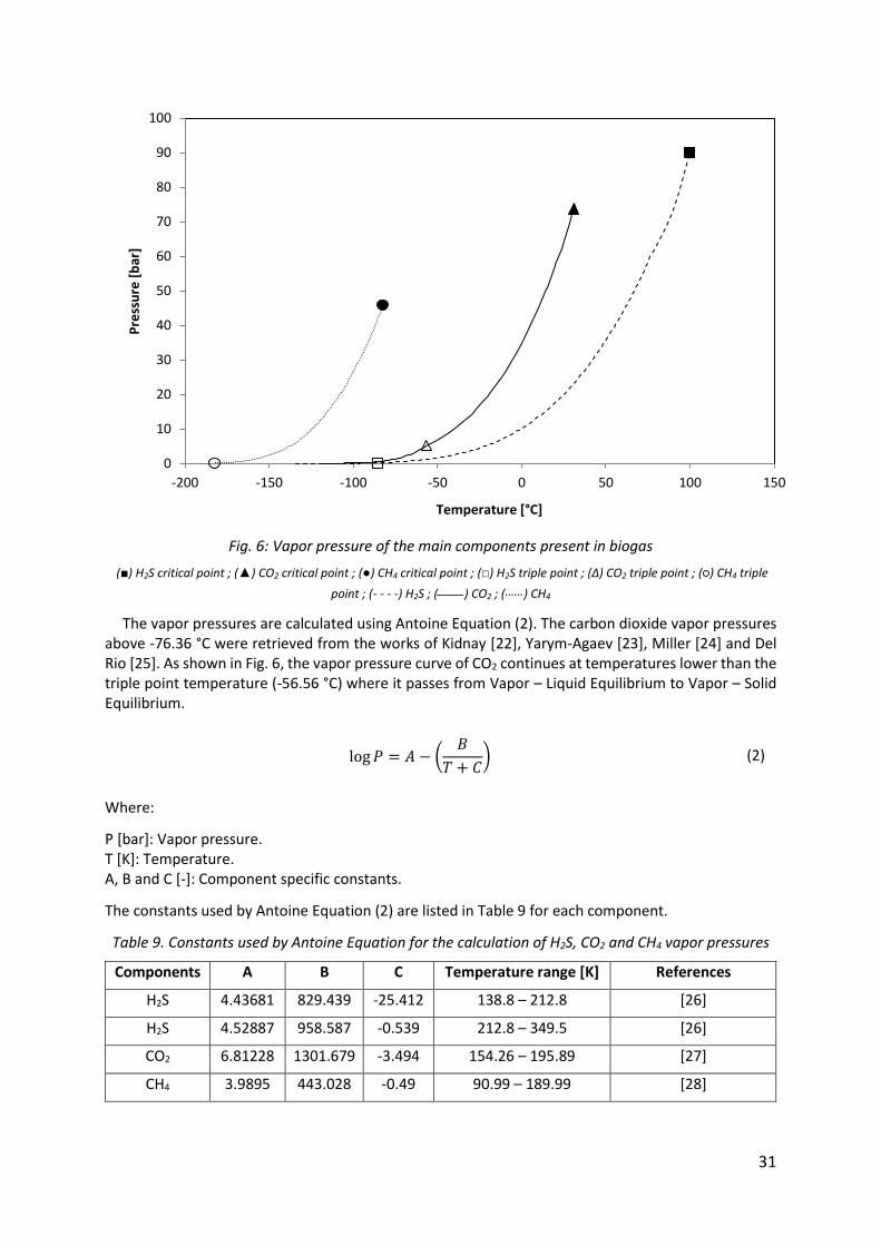
Fig. 6: Vapor pressure of the main components present in biogas
(■) H2S critical point ; (▲) CO2 critical point ; (●) CH4 critical point ; (□) H2S triple point ; (Δ) CO2 triple point ; (○) CH4 triple
point ; (- - - -) H2S ; (____) CO2 ; (……) CH4
The vapor pressures are calculated using Antoine Equation (2). The carbon dioxide vapor pressures above -76.36 °C were retrieved from the works of Kidnay [22], Yarym-Agaev [23], Miller [24] and Del Rio [25]. As shown in Fig. 6, the vapor pressure curve of CO2 continues at temperatures lower than the triple point temperature (-56.56 °C) where it passes from Vapor – Liquid Equilibrium to Vapor – Solid Equilibrium.
log 𝑃 = 𝐴 − (𝐵
𝑇 + 𝐶) (2)
Where:
P [bar]: Vapor pressure. T [K]: Temperature. A, B and C [-]: Component specific constants.
The constants used by Antoine Equation (2) are listed in Table 9 for each component.
Table 9. Constants used by Antoine Equation for the calculation of H2S, CO2 and CH4 vapor pressures
Components A B C Temperature range [K] References
H2S 4.43681 829.439 -25.412 138.8 – 212.8 [26]
H2S 4.52887 958.587 -0.539 212.8 – 349.5 [26]
CO2 6.81228 1301.679 -3.494 154.26 – 195.89 [27]
CH4 3.9895 443.028 -0.49 90.99 – 189.99 [28]
0
10
20
30
40
50
60
70
80
90
100
-200 -150 -100 -50 0 50 100 150
Pre
ssu
re [
bar
]
Temperature [°C]
32
2.3. Thermodynamic properties of the gas mixture (biogas)
2.3.1. Phase equilibrium behavior of biogas
In this section, the gas mixture is assumed to consist of methane (1) and carbon dioxide (2) because all the other impurities are present at very low concentrations depending on the type of substrate as shown in Table 4. Further, the upgrading process is generally made after purification that consists in the elimination of all these pollutants such as H2S, H2O and siloxanes.
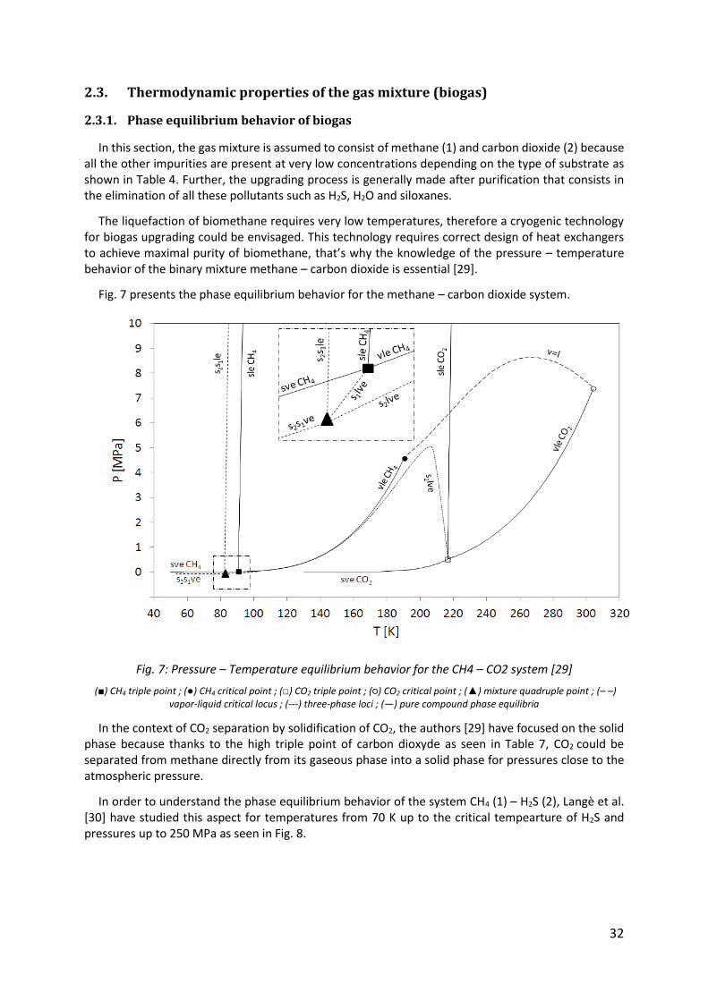
The liquefaction of biomethane requires very low temperatures, therefore a cryogenic technology for biogas upgrading could be envisaged. This technology requires correct design of heat exchangers to achieve maximal purity of biomethane, that’s why the knowledge of the pressure – temperature behavior of the binary mixture methane – carbon dioxide is essential [29].
Fig. 7 presents the phase equilibrium behavior for the methane – carbon dioxide system.
Fig. 7: Pressure – Temperature equilibrium behavior for the CH4 – CO2 system [29]
(■) CH4 triple point ; (●) CH4 critical point ; (□) CO2 triple point ; (○) CO2 critical point ; (▲) mixture quadruple point ; (– –) vapor-liquid critical locus ; (---) three-phase loci ; (—) pure compound phase equilibria
In the context of CO2 separation by solidification of CO2, the authors [29] have focused on the solid phase because thanks to the high triple point of carbon dioxyde as seen in Table 7, CO2 could be separated from methane directly from its gaseous phase into a solid phase for pressures close to the atmospheric pressure.
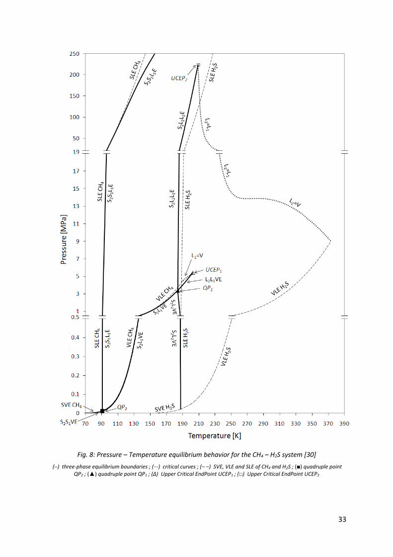
In order to understand the phase equilibrium behavior of the system CH4 (1) – H2S (2), Langè et al. [30] have studied this aspect for temperatures from 70 K up to the critical tempearture of H2S and pressures up to 250 MPa as seen in Fig. 8.
33
Fig. 8: Pressure – Temperature equilibrium behavior for the CH4 – H2S system [30]
(─) three-phase equilibrium boundaries ; (∙∙∙) critical curves ; (– –) SVE, VLE and SLE of CH4 and H2S ; (■) quadruple point QP2 ; (▲) quadruple point QP1 ; (Δ) Upper Critical EndPoint UCEP1 ; (□) Upper Critical EndPoint UCEP2

34
2.3.2. Density and dynamic viscosity of biogas
All the thermophysical properties discussed in this section are calculated using the software REFPROP V9.0 which calculates the thermodynamic and transport properties of industrially important fluids and their mixtures. The equation of state for calculating these properties is the GERG (European Gas Research Group) – 2008 equation [31].
Depending on its composition, biogas has characteristics that it is interesting to investigate such as density and viscosity.
At a pressure of 1,103 bar, slightly higher than the atmospheric pressure, the variation of density as a function of temperature is shown in Fig. 9.
Fig. 9: Biogas density as a function of temperature
(____) Air ; (……) Biogas with 40 mol% of CO2 ; (- - - -) Biogas with 35 mol% of CO2
As seen in Fig. 9, biogas is lighter than air. Moreover, its density depends on the carbon dioxide content. The density of a biogas rich on carbon dioxide will be greater than that of a biogas containing an inferior CO2 concentration. This is due to the molecular weight of CO2 which is greater than that of methane as seen in Tables 7 and 8.
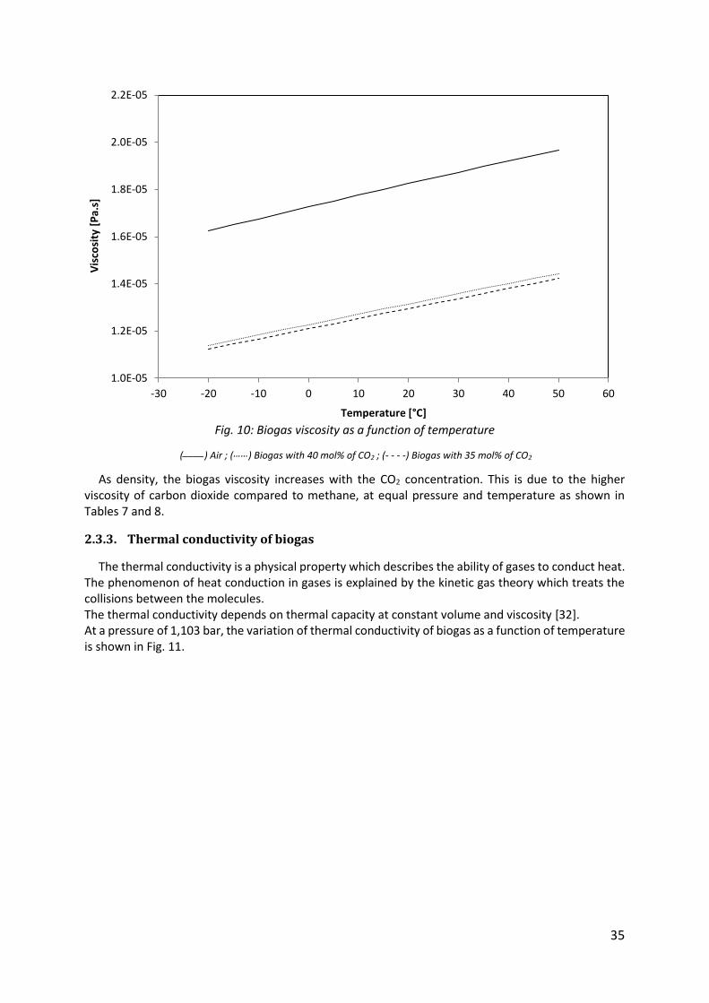
At a pressure of 1,103 bar, the evolution of the viscosity of the biogas as a function of temperature is depicted in Fig. 10.
1
1.1
1.2
1.3
1.4
1.5
1.6
-30 -20 -10 0 10 20 30 40 50 60
De
nsi
ty [
kg/m
3]
Temperature [°C]
35
Fig. 10: Biogas viscosity as a function of temperature
(____) Air ; (……) Biogas with 40 mol% of CO2 ; (- - - -) Biogas with 35 mol% of CO2
As density, the biogas viscosity increases with the CO2 concentration. This is due to the higher viscosity of carbon dioxide compared to methane, at equal pressure and temperature as shown in Tables 7 and 8.
2.3.3. Thermal conductivity of biogas
The thermal conductivity is a physical property which describes the ability of gases to conduct heat. The phenomenon of heat conduction in gases is explained by the kinetic gas theory which treats the collisions between the molecules. The thermal conductivity depends on thermal capacity at constant volume and viscosity [32]. At a pressure of 1,103 bar, the variation of thermal conductivity of biogas as a function of temperature is shown in Fig. 11.
1.0E-05
1.2E-05
1.4E-05
1.6E-05
1.8E-05
2.0E-05
2.2E-05
-30 -20 -10 0 10 20 30 40 50 60
Vis
cosi
ty [
Pa.
s]
Temperature [°C]
36
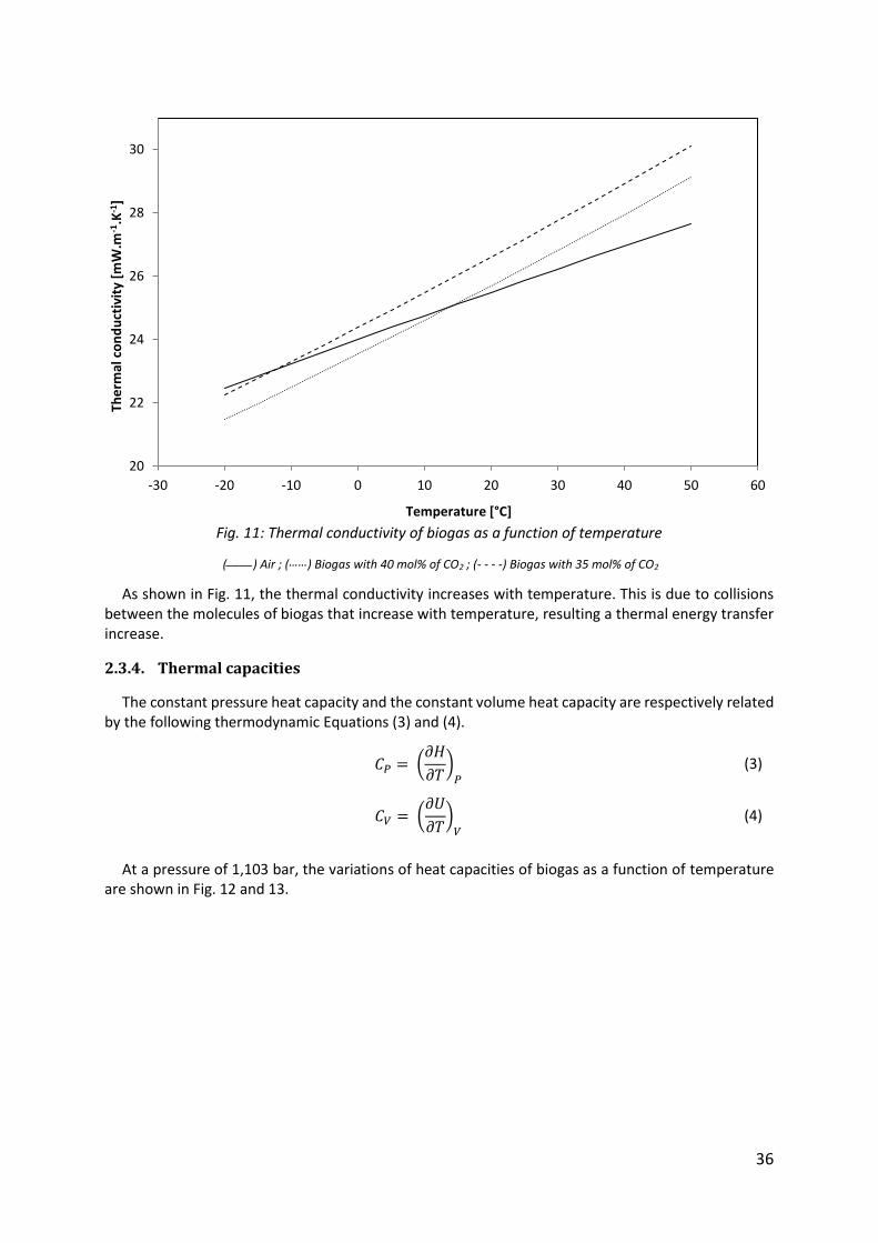
Fig. 11: Thermal conductivity of biogas as a function of temperature
(____) Air ; (……) Biogas with 40 mol% of CO2 ; (- - - -) Biogas with 35 mol% of CO2
As shown in Fig. 11, the thermal conductivity increases with temperature. This is due to collisions between the molecules of biogas that increase with temperature, resulting a thermal energy transfer increase.
2.3.4. Thermal capacities
The constant pressure heat capacity and the constant volume heat capacity are respectively related by the following thermodynamic Equations (3) and (4).
𝐶𝑃 = (𝜕𝐻
𝜕𝑇)
𝑃 (3)
𝐶𝑉 = (𝜕𝑈
𝜕𝑇)
𝑉 (4)
At a pressure of 1,103 bar, the variations of heat capacities of biogas as a function of temperature are shown in Fig. 12 and 13.
20
22
24
26
28
30
-30 -20 -10 0 10 20 30 40 50 60
The
rmal
co
nd
uct
ivit
y [m
W.m
-1.K
-1]
Temperature [°C]
37
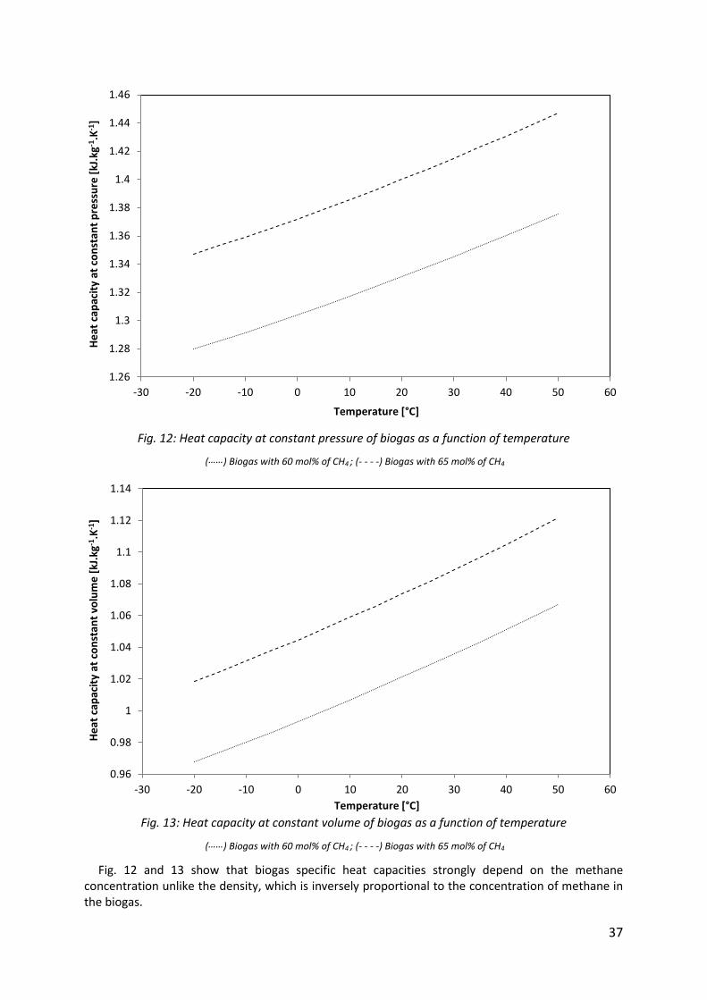
Fig. 12: Heat capacity at constant pressure of biogas as a function of temperature
(……) Biogas with 60 mol% of CH4 ; (- - - -) Biogas with 65 mol% of CH4
Fig. 13: Heat capacity at constant volume of biogas as a function of temperature
(……) Biogas with 60 mol% of CH4 ; (- - - -) Biogas with 65 mol% of CH4
Fig. 12 and 13 show that biogas specific heat capacities strongly depend on the methane concentration unlike the density, which is inversely proportional to the concentration of methane in the biogas.
1.26
1.28
1.3
1.32
1.34
1.36
1.38
1.4
1.42
1.44
1.46
-30 -20 -10 0 10 20 30 40 50 60
He
at c
apac
ity
at c
on
stan
t p
ress
ure
[kJ
.kg-1
.K-1
]
Temperature [°C]
0.96
0.98
1
1.02
1.04
1.06
1.08
1.1
1.12
1.14
-30 -20 -10 0 10 20 30 40 50 60
He
at c
apac
ity
at c
on
stan
t vo
lum
e [
kJ.k
g-1.K
-1]
Temperature [°C]

38
According to Vardanjan et al. [33], an increase of methane concentration from 50 % to 75 % will result in the increase of heat capacity by 17 %. In Fig. 12 and 13, heat capacities increased by 5 % after the passage of the methane concentration from 60 to 65 %.
2.4. Energy content in biogas
An important property of biogas is the lower heating value (LHV) which measures its energy value. The LHV of biogas is proportional to its methane content. For example, a biogas containing 70 mol% of methane at 15 °C and at atmospheric pressure has a LHV equal to 6.6 kWh/m3 [34].
The energy value of biogas can also be evaluated by the Wobbe Index. Compared to the calorific value of biogas which has been treated by a lot of authors, only few studies have been conducted on the Wobbe index of biogas. According to the Danish Technological Institute (DTI) [35], a biogas containing 60 mol% of methane, 38 mol% of carbon dioxide and 2 mol% of others has a Wobbe index of 19.5 MJ/m3.
2.5. Conclusion
This chapter has allowed identifying the thermophysical properties of biogas. These properties are essential to design and optimize technologies for biogas purification and upgrading.
The thermophysical properties of biogas discussed in this chapter strongly depend on the composition of biogas, especially the concentrations of methane and carbon dioxide.
The presence of minor compounds such as H2O, N2, O2 and H2S could change the physical properties of biogas. For example, landfill gas includes small amounts of nitrogen and oxygen which affect the phase behavior of the CH4 – CO2 system.
The technologies used for purification and upgrading of biogas will be discussed in the following section and a particular attention will be paid to the elimination of hydrogen sulfide.

39
Chapter 3: From molecules to the process Résumé :
La valorisation du biogaz nécessite la mise en œuvre d’un procédé de purification qui consiste à éliminer du biogaz brut toutes les substances indésirables afin d’augmenter au maximum sa teneur en méthane.
Ce chapitre présente une étude comparative des méthodes connues de séparation de H2S du biogaz. La méthode de séparation devra permettre de réduire la teneur résiduelle en H2S à moins de 1 ppm.
La première technique de séparation étudiée est l’absorption dans des contacteurs gaz – liquide. L’accent a été porté sur les principes fondamentaux basés sur l’absorption avec des solvants de type physique et chimique ainsi que leur efficacité dans l’élimination de l’H2S.
La deuxième technique de traitement de l’H2S étudiée est l’adsorption sur des solides microporeux comme le charbon actif et les zéolithes.
Le troisième procédé discuté est la séparation membranaire dont la performance dépend de deux paramètres qui sont : la perméabilité et la sélectivité membranaires. En général, les membranes de perméabilité élevée présentent une faible sélectivité et inversement. Cette méthode présente quelques inconvénients comme le risque de rupture dû au gradient de pression qui constitue la force motrice, l’exposition à certains solvants qui peut endommager ou boucher la membrane, le prix élevé des membranes ou encore les pertes en méthane qui peuvent être considérables.
La dernière technologie séparative étudiée lors de ce chapitre est la condensation cryogénique basée sur la thermodynamique des équilibres de phases.
Cette synthèse bibliographique a permis de comparer les différents procédés selon plusieurs critères comme l'efficacité de séparation, l'impact environnemental et les coûts d'investissement et d'exploitation.
Finalement, le choix s’est porté sur les deux technologies suivantes utilisées pour l'élimination du sulfure d'hydrogène:
• Absorption chimique dans une colonne à garnissage structuré utilisant l'hydroxyde de sodium (NaOH) comme solvant.
• Adsorption dans un lit fixe de charbon actif.
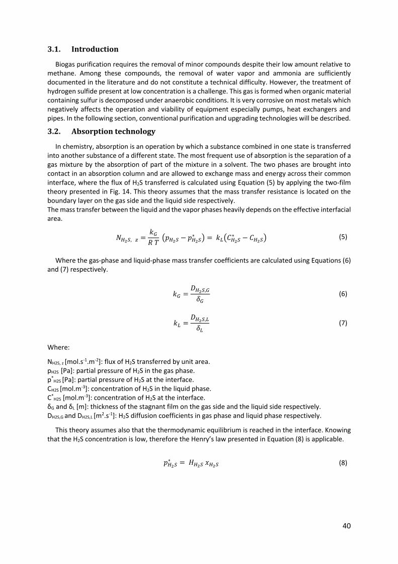
40
3.1. Introduction
Biogas purification requires the removal of minor compounds despite their low amount relative to methane. Among these compounds, the removal of water vapor and ammonia are sufficiently documented in the literature and do not constitute a technical difficulty. However, the treatment of hydrogen sulfide present at low concentration is a challenge. This gas is formed when organic material containing sulfur is decomposed under anaerobic conditions. It is very corrosive on most metals which negatively affects the operation and viability of equipment especially pumps, heat exchangers and pipes. In the following section, conventional purification and upgrading technologies will be described.
3.2. Absorption technology
In chemistry, absorption is an operation by which a substance combined in one state is transferred into another substance of a different state. The most frequent use of absorption is the separation of a gas mixture by the absorption of part of the mixture in a solvent. The two phases are brought into contact in an absorption column and are allowed to exchange mass and energy across their common interface, where the flux of H2S transferred is calculated using Equation (5) by applying the two-film theory presented in Fig. 14. This theory assumes that the mass transfer resistance is located on the boundary layer on the gas side and the liquid side respectively. The mass transfer between the liquid and the vapor phases heavily depends on the effective interfacial area.
𝑁𝐻2𝑆, 𝑧 =𝑘𝐺
𝑅 𝑇 (𝑝𝐻2𝑆 − 𝑝𝐻2𝑆
∗ ) = 𝑘𝐿(𝐶𝐻2𝑆∗ − 𝐶𝐻2𝑆) (5)
Where the gas-phase and liquid-phase mass transfer coefficients are calculated using Equations (6) and (7) respectively.
𝑘𝐺 =𝐷𝐻2𝑆,𝐺
𝛿𝐺 (6)
𝑘𝐿 =𝐷𝐻2𝑆,𝐿
𝛿𝐿 (7)
Where:
NH2S, z [mol.s-1.m-2]: flux of H2S transferred by unit area. pH2S [Pa]: partial pressure of H2S in the gas phase. p*
H2S [Pa]: partial pressure of H2S at the interface. CH2S [mol.m-3]: concentration of H2S in the liquid phase. C*
H2S [mol.m-3]: concentration of H2S at the interface. δG and δL [m]: thickness of the stagnant film on the gas side and the liquid side respectively. DH2S,G and DH2S,L [m2.s-1]: H2S diffusion coefficients in gas phase and liquid phase respectively.
This theory assumes also that the thermodynamic equilibrium is reached in the interface. Knowing that the H2S concentration is low, therefore the Henry’s law presented in Equation (8) is applicable.
𝑝𝐻2𝑆∗ = 𝐻𝐻2𝑆 𝑥𝐻2𝑆 (8)
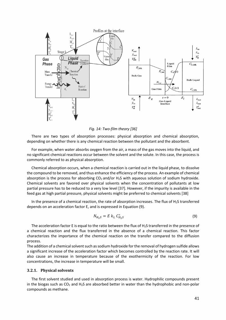
41
Fig. 14: Two-film theory [36]
There are two types of absorption processes: physical absorption and chemical absorption, depending on whether there is any chemical reaction between the pollutant and the absorbent.
For example, when water absorbs oxygen from the air, a mass of the gas moves into the liquid, and no significant chemical reactions occur between the solvent and the solute. In this case, the process is commonly referred to as physical absorption.
Chemical absorption occurs, when a chemical reaction is carried out in the liquid phase, to dissolve the compound to be removed, and thus enhance the efficiency of the process. An example of chemical absorption is the process for absorbing CO2 and/or H2S with aqueous solution of sodium hydroxide. Chemical solvents are favored over physical solvents when the concentration of pollutants at low partial pressure has to be reduced to a very low level [37]. However, if the impurity is available in the feed gas at high partial pressure, physical solvents might be preferred to chemical solvents [38]
In the presence of a chemical reaction, the rate of absorption increases. The flux of H2S transferred depends on an acceleration factor E, and is expressed in Equation (9).
𝑁𝐻2𝑆 = 𝐸 𝑘𝐿 𝐶𝐻2𝑆∗ (9)
The acceleration factor E is equal to the ratio between the flux of H2S transferred in the presence of a chemical reaction and the flux transferred in the absence of a chemical reaction. This factor characterizes the importance of the chemical reaction on the transfer compared to the diffusion process. The addition of a chemical solvent such as sodium hydroxide for the removal of hydrogen sulfide allows a significant increase of the acceleration factor which becomes controlled by the reaction rate. It will also cause an increase in temperature because of the exothermicity of the reaction. For low concentrations, the increase in temperature will be small.
3.2.1. Physical solvents
The first solvent studied and used in absorption process is water. Hydrophilic compounds present in the biogas such as CO2 and H2S are absorbed better in water than the hydrophobic and non-polar compounds as methane.

42
Table 10 shows the solubility of some compounds of biogas in water.
Table 10. Solubility of the main compounds of biogas in water [39]
Compound Solubility in water at 1 bar of partial pressure
[mg.l-1] at 0 °C [mg.l-1] at 25 °C
NH3 53 000 28 000
H2S 205 102
CO2 75 34
CH4 2.45 1.32
Siloxanes < 1 < 1
In order to improve the effectiveness of absorption processes, other solvents were tested for purification and upgrading of biogas. They allow the reduction of the size of columns, the energy used for the treatment and the volumes of solvents involved.
Selexol® is a physical absorption process developed by Allied Chemical Corporation, then improved by Norton. Today, it is owned by Universal Oil Products (UOP). It is made up of Dimethyl Ethers of Polyethylene Glycol (DMEPG) whose molecular weight is about 272 g.mol-1.
Rectisol® is one of the older physical absorption processes. It was developed by Linde and Lurgi in order to separate the acid gases present in the syngas from gasification of coal. It has also been used for separation of CO2 in the syngas of units producing hydrogen and ammonia. This process uses a methanol-based solvent (MeOH) whose chemical formula is CH3OH.
These solvents exhibit a high selectivity for H2S removal compared to the other compounds, in particular CO2. Other processes exist such as Purisol® based on the use of N-Methyl-2-Pyrrolidone (NMP), and Morphysorb® destined for the separation of acid gases at high concentrations, using N-Formyl-Morpholine (NFM). The main physical solvents are summarized in Table 11 where selected physical properties are compared.
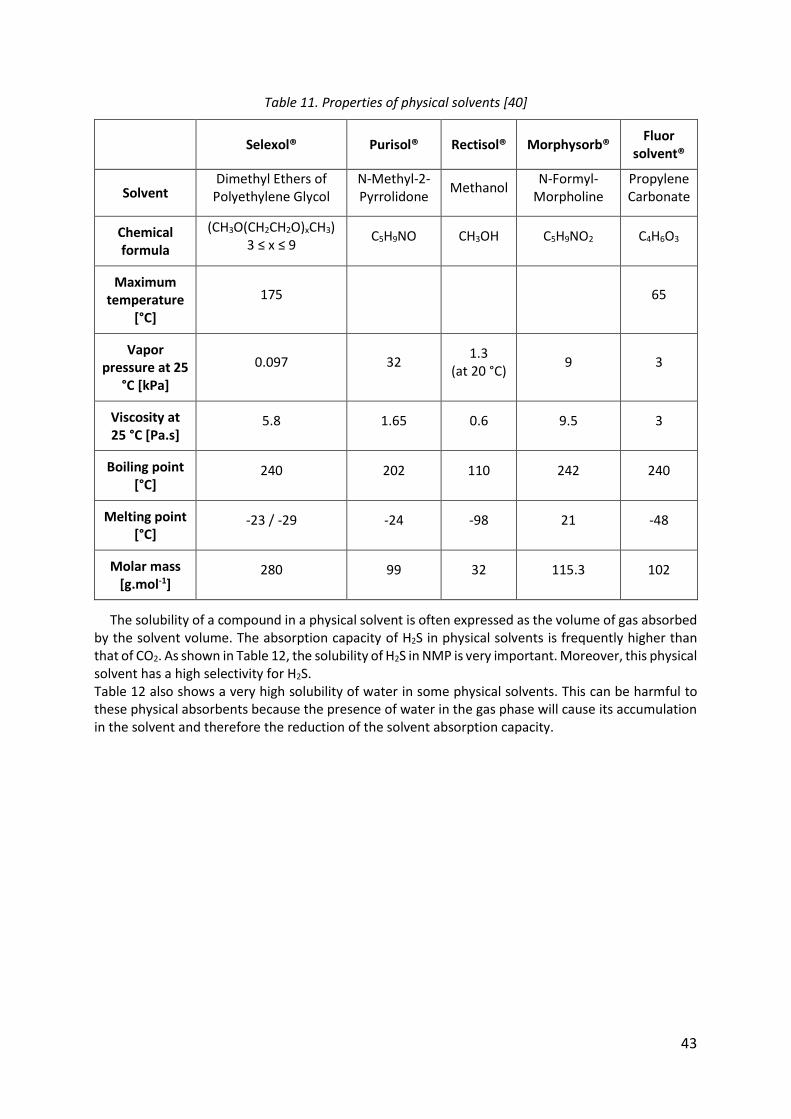
43
Table 11. Properties of physical solvents [40]
Selexol® Purisol® Rectisol® Morphysorb® Fluor
solvent®
Solvent Dimethyl Ethers of
Polyethylene Glycol N-Methyl-2-Pyrrolidone
Methanol N-Formyl-
Morpholine Propylene Carbonate
Chemical formula
(CH3O(CH2CH2O)xCH3) 3 ≤ x ≤ 9
C5H9NO CH3OH C5H9NO2 C4H6O3
Maximum temperature
[°C]
175 65
Vapor pressure at 25
°C [kPa]
0.097 32 1.3
(at 20 °C) 9 3
Viscosity at 25 °C [Pa.s]
5.8 1.65 0.6 9.5 3
Boiling point [°C]
240 202 110 242 240
Melting point [°C]
-23 / -29 -24 -98 21 -48
Molar mass [g.mol-1]
280 99 32 115.3 102
The solubility of a compound in a physical solvent is often expressed as the volume of gas absorbed by the solvent volume. The absorption capacity of H2S in physical solvents is frequently higher than that of CO2. As shown in Table 12, the solubility of H2S in NMP is very important. Moreover, this physical solvent has a high selectivity for H2S. Table 12 also shows a very high solubility of water in some physical solvents. This can be harmful to these physical absorbents because the presence of water in the gas phase will cause its accumulation in the solvent and therefore the reduction of the solvent absorption capacity.
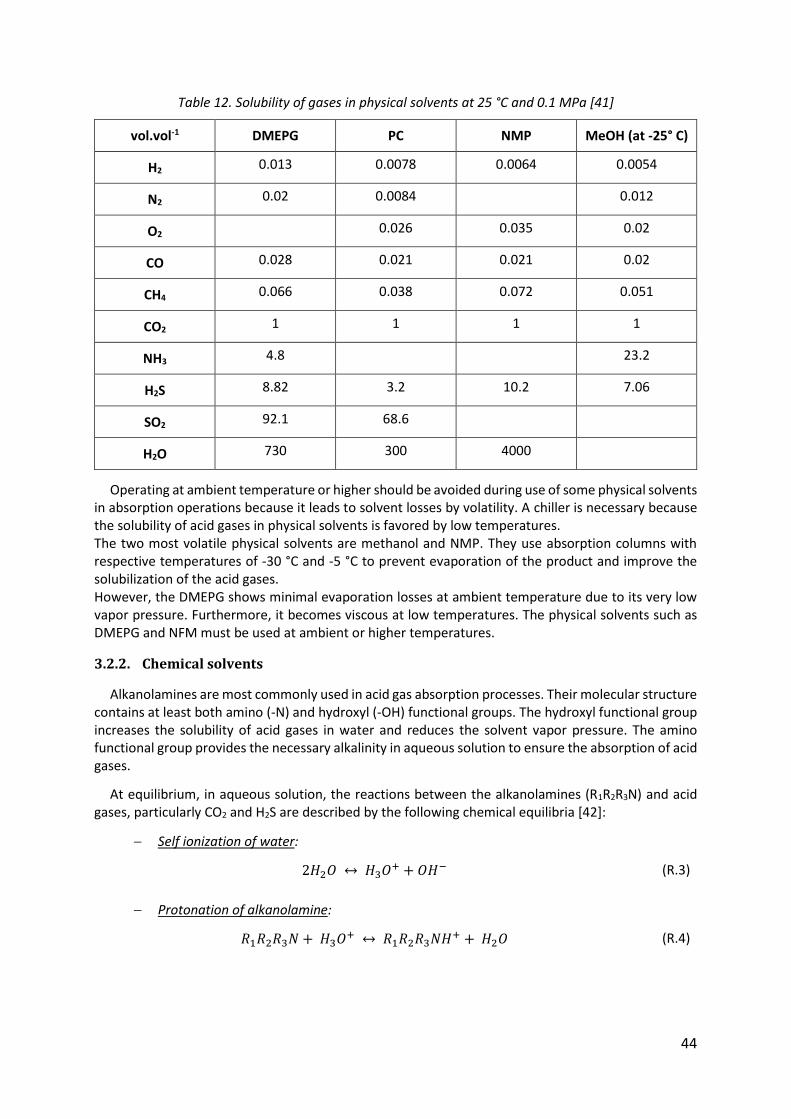
44
Table 12. Solubility of gases in physical solvents at 25 °C and 0.1 MPa [41]
vol.vol-1 DMEPG PC NMP MeOH (at -25° C)
H2 0.013 0.0078 0.0064 0.0054
N2 0.02 0.0084 0.012
O2 0.026 0.035 0.02
CO 0.028 0.021 0.021 0.02
CH4 0.066 0.038 0.072 0.051
CO2 1 1 1 1
NH3 4.8 23.2
H2S 8.82 3.2 10.2 7.06
SO2 92.1 68.6
H2O 730 300 4000
Operating at ambient temperature or higher should be avoided during use of some physical solvents in absorption operations because it leads to solvent losses by volatility. A chiller is necessary because the solubility of acid gases in physical solvents is favored by low temperatures. The two most volatile physical solvents are methanol and NMP. They use absorption columns with respective temperatures of -30 °C and -5 °C to prevent evaporation of the product and improve the solubilization of the acid gases. However, the DMEPG shows minimal evaporation losses at ambient temperature due to its very low vapor pressure. Furthermore, it becomes viscous at low temperatures. The physical solvents such as DMEPG and NFM must be used at ambient or higher temperatures.
3.2.2. Chemical solvents
Alkanolamines are most commonly used in acid gas absorption processes. Their molecular structure contains at least both amino (-N) and hydroxyl (-OH) functional groups. The hydroxyl functional group increases the solubility of acid gases in water and reduces the solvent vapor pressure. The amino functional group provides the necessary alkalinity in aqueous solution to ensure the absorption of acid gases.
At equilibrium, in aqueous solution, the reactions between the alkanolamines (R1R2R3N) and acid gases, particularly CO2 and H2S are described by the following chemical equilibria [42]:
Self ionization of water:
2𝐻2𝑂 ↔ 𝐻3𝑂+ + 𝑂𝐻− (R.3)
Protonation of alkanolamine:
𝑅1𝑅2𝑅3𝑁 + 𝐻3𝑂+ ↔ 𝑅1𝑅2𝑅3𝑁𝐻+ + 𝐻2𝑂 (R.4)
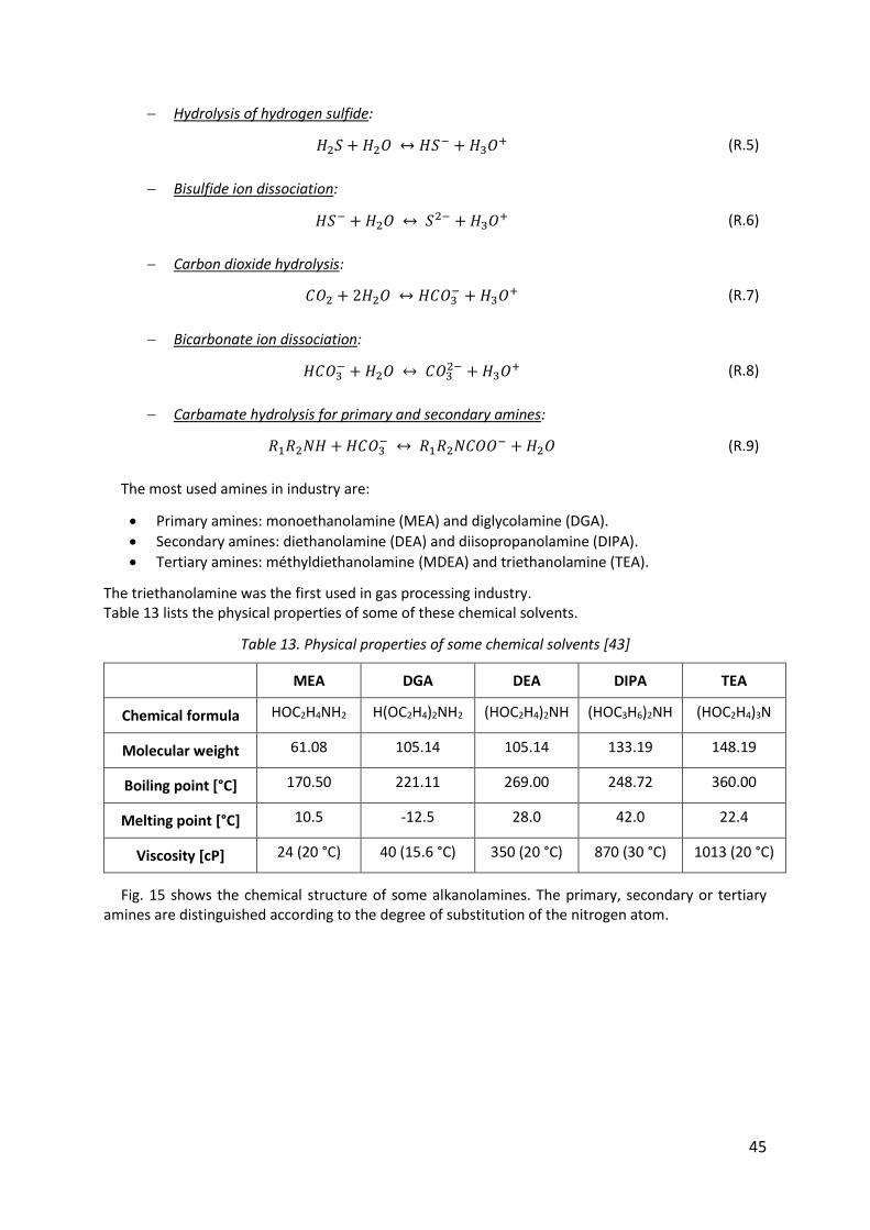
45
Hydrolysis of hydrogen sulfide:
𝐻2𝑆 + 𝐻2𝑂 ↔ 𝐻𝑆− + 𝐻3𝑂+ (R.5)
Bisulfide ion dissociation:
𝐻𝑆− + 𝐻2𝑂 ↔ 𝑆2− + 𝐻3𝑂+ (R.6)
Carbon dioxide hydrolysis:
𝐶𝑂2 + 2𝐻2𝑂 ↔ 𝐻𝐶𝑂3− + 𝐻3𝑂+ (R.7)
Bicarbonate ion dissociation:
𝐻𝐶𝑂3− + 𝐻2𝑂 ↔ 𝐶𝑂3
2− + 𝐻3𝑂+ (R.8)
Carbamate hydrolysis for primary and secondary amines:
𝑅1𝑅2𝑁𝐻 + 𝐻𝐶𝑂3− ↔ 𝑅1𝑅2𝑁𝐶𝑂𝑂− + 𝐻2𝑂 (R.9)
The most used amines in industry are:
Primary amines: monoethanolamine (MEA) and diglycolamine (DGA).
Secondary amines: diethanolamine (DEA) and diisopropanolamine (DIPA).
Tertiary amines: méthyldiethanolamine (MDEA) and triethanolamine (TEA).
The triethanolamine was the first used in gas processing industry. Table 13 lists the physical properties of some of these chemical solvents.
Table 13. Physical properties of some chemical solvents [43]
MEA DGA DEA DIPA TEA
Chemical formula HOC2H4NH2 H(OC2H4)2NH2 (HOC2H4)2NH (HOC3H6)2NH (HOC2H4)3N
Molecular weight 61.08 105.14 105.14 133.19 148.19
Boiling point [°C] 170.50 221.11 269.00 248.72 360.00
Melting point [°C] 10.5 -12.5 28.0 42.0 22.4
Viscosity [cP] 24 (20 °C) 40 (15.6 °C) 350 (20 °C) 870 (30 °C) 1013 (20 °C)
Fig. 15 shows the chemical structure of some alkanolamines. The primary, secondary or tertiary amines are distinguished according to the degree of substitution of the nitrogen atom.
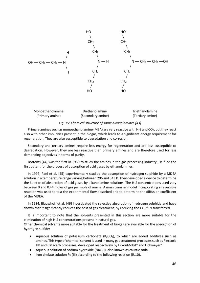
46
Monoethanolamine (Primary amine)
Diethanolamine (Secondary amine)
Triethanolamine (Tertiary amine)
Fig. 15: Chemical structure of some alkanolamines [43]
Primary amines such as monoethanolamine (MEA) are very reactive with H2S and CO2, but they react also with other impurities present in the biogas, which leads to a significant energy requirement for regeneration. They are also susceptible to degradation and corrosion.
Secondary and tertiary amines require less energy for regeneration and are less susceptible to degradation. However, they are less reactive than primary amines and are therefore used for less demanding objectives in terms of purity.
Bottoms [44] was the first in 1930 to study the amines in the gas processing industry. He filed the first patent for the process of absorption of acid gases by ethanolamines.
In 1997, Pani et al. [45] experimentally studied the absorption of hydrogen sulphide by a MDEA solution in a temperature range varying between 296 and 343 K. They developed a device to determine the kinetics of absorption of acid gases by alkanolamine solutions, The H2S concentrations used vary between 0 and 0.44 moles of gas per mole of amine. A mass transfer model incorporating a reversible reaction was used to test the experimental flow absorbed and to determine the diffusion coefficient of the MDEA.
In 1984, Blauwhoff et al. [46] investigated the selective absorption of hydrogen sulphide and have shown that it significantly reduces the cost of gas treatment, by reducing the CO2 flux transferred.
It is important to note that the solvents presented in this section are more suitable for the elimination of high H2S concentrations present in natural gas. Other chemical solvents more suitable for the treatment of biogas are available for the absorption of hydrogen sulfide:
Aqueous solution of potassium carbonate (K2CO3), to which are added additives such as amines. This type of chemical solvent is used in many gas treatment processes such as Flexsorb HP and Catacarb processes, developed respectively by ExxonMobil® and Eickmeyer®.
Aqueous solution of sodium hydroxide (NaOH), also known as caustic soda.
Iron chelate solution Fe (III) according to the following reaction (R.10).
H / OH ― CH2 ― CH2 ― N \ H
HO \ CH2 \ CH2 \ N ― H / CH2 / CH2 / HO
HO \ CH2 \ CH2 \ N ― CH2 ― CH2 ―OH / CH2 / CH2 / HO
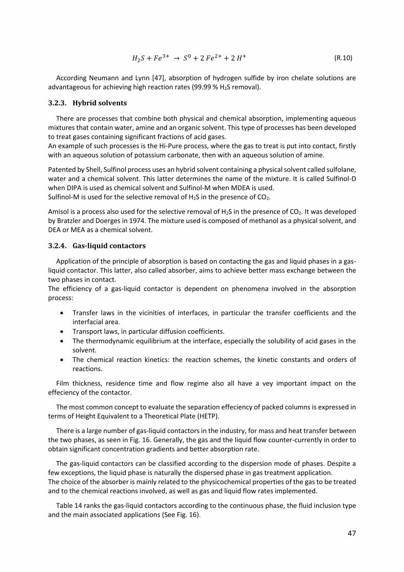
47
𝐻2𝑆 + 𝐹𝑒3+ → 𝑆0 + 2 𝐹𝑒2+ + 2 𝐻+ (R.10)
According Neumann and Lynn [47], absorption of hydrogen sulfide by iron chelate solutions are advantageous for achieving high reaction rates (99.99 % H2S removal).
3.2.3. Hybrid solvents
There are processes that combine both physical and chemical absorption, implementing aqueous mixtures that contain water, amine and an organic solvent. This type of processes has been developed to treat gases containing significant fractions of acid gases. An example of such processes is the Hi-Pure process, where the gas to treat is put into contact, firstly with an aqueous solution of potassium carbonate, then with an aqueous solution of amine.
Patented by Shell, Sulfinol process uses an hybrid solvent containing a physical solvent called sulfolane, water and a chemical solvent. This latter determines the name of the mixture. It is called Sulfinol-D when DIPA is used as chemical solvent and Sulfinol-M when MDEA is used. Sulfinol-M is used for the selective removal of H2S in the presence of CO2.
Amisol is a process also used for the selective removal of H2S in the presence of CO2. It was developed by Bratzler and Doerges in 1974. The mixture used is composed of methanol as a physical solvent, and DEA or MEA as a chemical solvent.
3.2.4. Gas-liquid contactors
Application of the principle of absorption is based on contacting the gas and liquid phases in a gas-liquid contactor. This latter, also called absorber, aims to achieve better mass exchange between the two phases in contact. The efficiency of a gas-liquid contactor is dependent on phenomena involved in the absorption process:
Transfer laws in the vicinities of interfaces, in particular the transfer coefficients and the interfacial area.
Transport laws, in particular diffusion coefficients.
The thermodynamic equilibrium at the interface, especially the solubility of acid gases in the solvent.
The chemical reaction kinetics: the reaction schemes, the kinetic constants and orders of reactions.
Film thickness, residence time and flow regime also all have a vey important impact on the effeciency of the contactor.
The most common concept to evaluate the separation effeciency of packed columns is expressed in terms of Height Equivalent to a Theoretical Plate (HETP).
There is a large number of gas-liquid contactors in the industry, for mass and heat transfer between the two phases, as seen in Fig. 16. Generally, the gas and the liquid flow counter-currently in order to obtain significant concentration gradients and better absorption rate.
The gas-liquid contactors can be classified according to the dispersion mode of phases. Despite a few exceptions, the liquid phase is naturally the dispersed phase in gas treatment application. The choice of the absorber is mainly related to the physicochemical properties of the gas to be treated and to the chemical reactions involved, as well as gas and liquid flow rates implemented.
Table 14 ranks the gas-liquid contactors according to the continuous phase, the fluid inclusion type and the main associated applications (See Fig. 16).
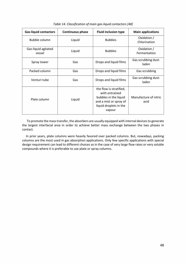
48
Table 14. Classification of main gas-liquid contactors [48]
Gas-liquid contactors Continuous phase Fluid inclusion type Main applications
Bubble column Liquid Bubbles Oxidation /
Chlorination
Gas-liquid agitated vessel
Liquid Bubbles Oxidation /
Fermentation
Spray tower Gas Drops and liquid films Gas scrubbing dust-
laden
Packed column Gas Drops and liquid films Gas scrubbing
Venturi tube Gas Drops and liquid films Gas scrubbing dust-
laden
Plate column Liquid
the flow is stratified, with entrained
bubbles in the liquid and a mist or spray of liquid droplets in the
vapour
Manufacture of nitric acid
To promote the mass transfer, the absorbers are usually equipped with internal devices to generate
the largest interfacial area in order to achieve better mass exchange between the two phases in contact.
In prior years, plate columns were heavily favored over packed columns. But, nowadays, packing columns are the most used in gas absorption applications. Only few specific applications with special design requirement can lead to different choices as in the case of very large flow rates or very soluble compounds where it is preferable to use plate or spray columns.

49
Fig. 16: Main gas-liquid contactors [48]
In a packed column, the gas and liquid normally flow counter currently as seen in Fig. 17. The liquid is sprayed from the top of the column to flow by gravity on the packing forming a large-area liquid film. The liquid enters in contact with the gas injected from the bottom of the column. Liquid flow must be sufficient to ensure uniform wetting of the packing and must not exceed a certain threshold in order to avoid flooding of the column.
The selection of the packing type and material is a very important issue in packed column design. The material should respect certain requirements as weight, pressure drop and especially corrosion resistance.
Fig. 17: Schematic representation of a packed column
Gas outlet
Liquid inlet
Liquid outlet
Packing
Gas inlet
Distributor
Support
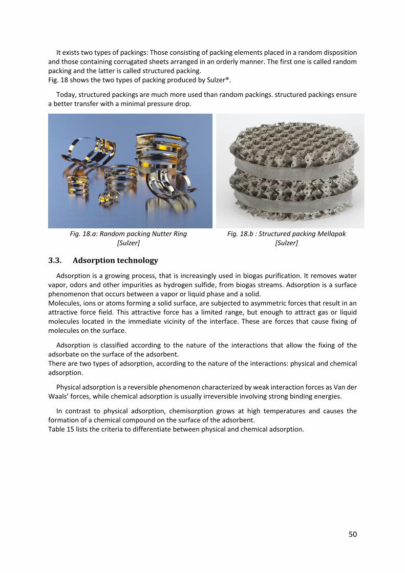
50
It exists two types of packings: Those consisting of packing elements placed in a random disposition and those containing corrugated sheets arranged in an orderly manner. The first one is called random packing and the latter is called structured packing. Fig. 18 shows the two types of packing produced by Sulzer®.
Today, structured packings are much more used than random packings. structured packings ensure a better transfer with a minimal pressure drop.
Fig. 18.a: Random packing Nutter Ring
[Sulzer] Fig. 18.b : Structured packing Mellapak
[Sulzer]
3.3. Adsorption technology
Adsorption is a growing process, that is increasingly used in biogas purification. It removes water vapor, odors and other impurities as hydrogen sulfide, from biogas streams. Adsorption is a surface phenomenon that occurs between a vapor or liquid phase and a solid. Molecules, ions or atoms forming a solid surface, are subjected to asymmetric forces that result in an attractive force field. This attractive force has a limited range, but enough to attract gas or liquid molecules located in the immediate vicinity of the interface. These are forces that cause fixing of molecules on the surface.
Adsorption is classified according to the nature of the interactions that allow the fixing of the adsorbate on the surface of the adsorbent. There are two types of adsorption, according to the nature of the interactions: physical and chemical adsorption.
Physical adsorption is a reversible phenomenon characterized by weak interaction forces as Van der Waals’ forces, while chemical adsorption is usually irreversible involving strong binding energies.
In contrast to physical adsorption, chemisorption grows at high temperatures and causes the formation of a chemical compound on the surface of the adsorbent. Table 15 lists the criteria to differentiate between physical and chemical adsorption.

51
Table 15. Criteria to differentiate between physical and chemical adsorption [49]
Criteria Physical adsorption Chemical adsorption
Process temperature Low High
Type of bond Van der Waals Chemical
Interaction forces 30 to 40 kJ.mol-1 80 to 800 kJ.mol-1
Layers Monolayers or multilayers Monolayers only
Kinetic Fast and reversible Slow and irreversible
Desorption Easy Difficult
3.3.1. Mechanism of adsorption
During adsorption process, the fluid molecules bind to the surface of a solid following three steps, describing the mass transfer from the fluid phase to the solid surface.
During the first step called external diffusion, the molecules of the fluid phase migrate to the vicinity of the outer surface of the solid particles. To model the transfer of the fluid phase towards the outer surface of the solid phase, the Equation (10) is often used:
−𝑑𝐶𝑡
𝑑𝑡= 𝑘𝑓 (
𝑎𝑎𝑑𝑠
𝑉) (𝐶𝑡 − 𝐶𝑒) (10)
Where:
Ct [mol.m-3]: the concentration of the compound in the fluid phase.
Ce [mol.m-3]: the concentration of the compound at the surface of the adsorbent. kf [m.s-1]: the external mass transfer coefficient. aads [m2]: the useful surface area for external transfer. V [m3]: Volume of the adsorption bed.
The second step is called internal diffusion. It results from the transfer of fluid phase particles from the outside of the solid surface inside the pores. To simplify the problem to one spatial dimension, the pore is assumed spherical. The flow transferred into the pore is expressed by Equation (11).
𝐽 = −𝐷𝑝 휀𝑝
𝜏 𝜕𝐶𝑝
𝜕𝑟 (11)
Where:
J [mol.m-2.s-1]: the transferred flux. Dp [m2.s-1]: the pore diffusion coefficient. ɛp [-]: the porosity. τ [-]: the tortuosity. Cp [mol.m-3]: the compound concentration in the pore. r [m]: radius of the pore.
The last step of the adsorption mechanism is the surface diffusion. It corresponds to the attachment of the vapor phase particles on the surface of the adsorbent. This step is very quick and independent of the overall process. The flux is then defined by Equation (12).
52
𝐽 = −𝐷𝑠 휀𝑝
𝜏 𝜕𝑞
𝜕𝑟 (12)
Where Ds [m2.s-1] is the surface diffusivity and q [mol.kg-1] is the amount adsorbed.
Fig. 19 shows the different steps of the adsorption mechanism.
Fig. 19: Transport mechanism of the adsorbate molecules on the adsorbent surface
3.3.2. Materials used for H2S adsorption
The adsorbents are microporous solids, characterized by high surface area per unit weight, from 100 to over 2000 m2.g-1. The classification of the International Union of Pure and Applied Chemistry (IUPAC) defines three kinds of pores by their size:
Microporous materials have pore diameters of less than 2 nm.
Mesoporous materials have pore diameters between 2 and 50 nm.
Macroporous materials have pore diameters of greater than 50 nm.
The most widely used adsorbents in industry remain: activated carbon, zeolite, silica gel and activated alumina. Other materials rarely used today as red mud may have good adsorption performance in H2S removal.
Activated carbon
Activated carbon is characterized by a high degree of microporosity. This structure gives the activated carbon its very large surface area. This essential feature allows the activated carbon to be by far, the most widely used adsorbent in industry. Pores size between of 0.5 and 1 nm were found by Yan et al. [50] to have the best adsorption capacity.
Activated carbon is characterized by a non-polar surface allowing it to preferentially adsorb non-polar compounds.
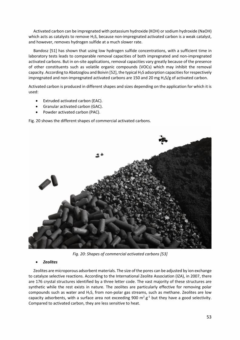
53
Activated carbon can be impregnated with potassium hydroxide (KOH) or sodium hydroxide (NaOH) which acts as catalysts to remove H2S, because non-impregnated activated carbon is a weak catalyst, and however, removes hydrogen sulfide at a much slower rate.
Bandosz [51] has shown that using low hydrogen sulfide concentrations, with a sufficient time in laboratory tests leads to comparable removal capacities of both impregnated and non-impregnated activated carbons. But in on-site applications, removal capacities vary greatly because of the presence of other constituents such as volatile organic compounds (VOCs) which may inhibit the removal capacity. According to Abatzoglou and Boivin [52], the typical H2S adsorption capacities for respectively impregnated and non-impregnated activated carbons are 150 and 20 mg H2S/g of activated carbon.
Activated carbon is produced in different shapes and sizes depending on the application for which it is used:
Extruded activated carbon (EAC).
Granular activated carbon (GAC).
Powder activated carbon (PAC).
Fig. 20 shows the different shapes of commercial activated carbons.
Fig. 20: Shapes of commercial activated carbons [53]
Zeolites
Zeolites are microporous adsorbent materials. The size of the pores can be adjusted by ion exchange to catalyze selective reactions. According to the International Zeolite Association (IZA), in 2007, there are 176 crystal structures identified by a three letter code. The vast majority of these structures are synthetic while the rest exists in nature. The zeolites are particularly effective for removing polar compounds such as water and H2S, from non-polar gas streams, such as methane. Zeolites are low capacity adsorbents, with a surface area not exceeding 900 m2.g-1 but they have a good selectivity. Compared to activated carbon, they are less sensitive to heat.

54
The adsorption of H2S present in biogas is one of the application envisaged with zeolites. The measured adsorption capacities remain well below the purification yields obtainable with other systems. Yasyerli et al. [54] determined an adsorption capacity of 30 mg.g-1 with clinoptilolite, a natural zeolite during the treatment of a real biogas. Cosoli et al. [55] reported an adsorption capacity of 40 mg.g-1 on synthetic zeolites, for H2S concentration of 1000 mg.m-3.
3.3.3. Factors affecting the adsorption
Literature concerning the factors affecting adsorption dates back to 1914 [56]. The main factors affecting the adsorption rate are the temperature, the surface area and the porosity of the adsorbent, the competition between species, and the polarity of the adsorbent and the adsorbate.
Temperature
Fig. 21 shows that during adsorption processes, the adsorbed amount increases as the temperature decreases. Moreover, physisorption releases heat. So, as any exothermic reaction, it is favored by low temperatures.
Fig. 21: Effect of temperature on some adsorbents [57]
Adsorbents: (───) Molecular sieves ; ( ─ ─ ─ ) Activated alumina ; (…….) Silica gel
Unlike physical adsorption, chemical adsorption requires higher temperatures, because it is an endothermic phenomenon.
Specific surface area
Adsorption performance increases with the specific surface area of the adsorbent. This proportionality was demonstrated by Bouchemal and Achour [58] during adsorption study of tyrosine on activated carbon.
0
5
10
15
20
25
30
0 100 200 300 400 500 600
Wat
er
adso
rbe
d [
lb/1
00
lb]
Temperature [°F]
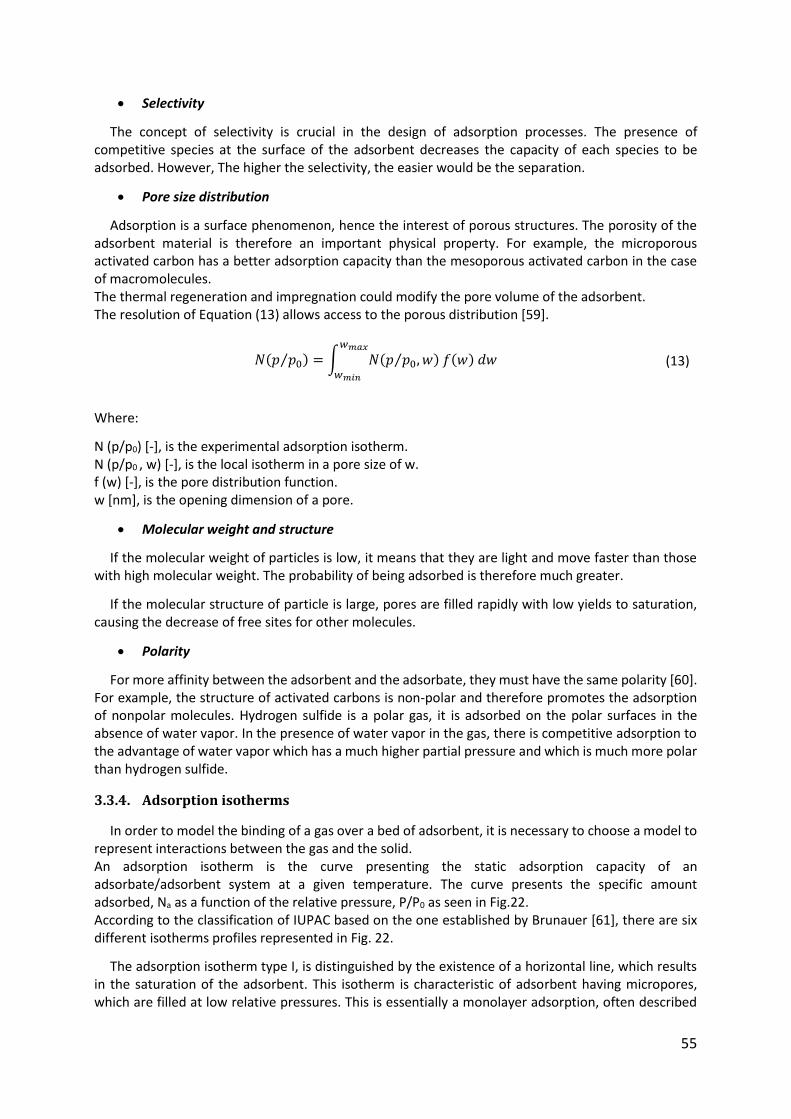
55
Selectivity
The concept of selectivity is crucial in the design of adsorption processes. The presence of competitive species at the surface of the adsorbent decreases the capacity of each species to be adsorbed. However, The higher the selectivity, the easier would be the separation.
Pore size distribution
Adsorption is a surface phenomenon, hence the interest of porous structures. The porosity of the adsorbent material is therefore an important physical property. For example, the microporous activated carbon has a better adsorption capacity than the mesoporous activated carbon in the case of macromolecules. The thermal regeneration and impregnation could modify the pore volume of the adsorbent. The resolution of Equation (13) allows access to the porous distribution [59].
𝑁(𝑝 𝑝0⁄ ) = ∫ 𝑁(𝑝 𝑝0, 𝑤⁄ ) 𝑓(𝑤) 𝑑𝑤𝑤𝑚𝑎𝑥
𝑤𝑚𝑖𝑛
(13)
Where:
N (p/p0) [-], is the experimental adsorption isotherm. N (p/p0 , w) [-], is the local isotherm in a pore size of w. f (w) [-], is the pore distribution function. w [nm], is the opening dimension of a pore.
Molecular weight and structure
If the molecular weight of particles is low, it means that they are light and move faster than those with high molecular weight. The probability of being adsorbed is therefore much greater.
If the molecular structure of particle is large, pores are filled rapidly with low yields to saturation, causing the decrease of free sites for other molecules.
Polarity
For more affinity between the adsorbent and the adsorbate, they must have the same polarity [60]. For example, the structure of activated carbons is non-polar and therefore promotes the adsorption of nonpolar molecules. Hydrogen sulfide is a polar gas, it is adsorbed on the polar surfaces in the absence of water vapor. In the presence of water vapor in the gas, there is competitive adsorption to the advantage of water vapor which has a much higher partial pressure and which is much more polar than hydrogen sulfide.
3.3.4. Adsorption isotherms
In order to model the binding of a gas over a bed of adsorbent, it is necessary to choose a model to represent interactions between the gas and the solid. An adsorption isotherm is the curve presenting the static adsorption capacity of an adsorbate/adsorbent system at a given temperature. The curve presents the specific amount adsorbed, Na as a function of the relative pressure, P/P0 as seen in Fig.22. According to the classification of IUPAC based on the one established by Brunauer [61], there are six different isotherms profiles represented in Fig. 22.
The adsorption isotherm type I, is distinguished by the existence of a horizontal line, which results in the saturation of the adsorbent. This isotherm is characteristic of adsorbent having micropores, which are filled at low relative pressures. This is essentially a monolayer adsorption, often described
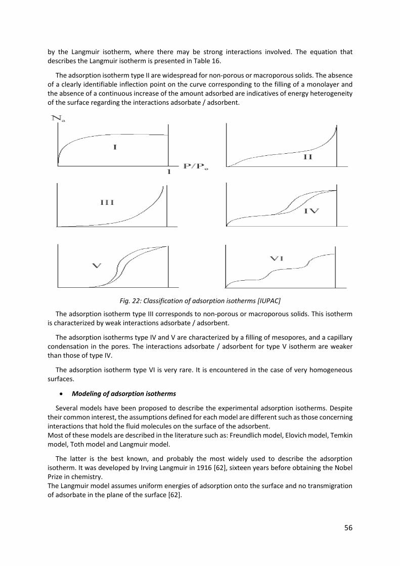
56
by the Langmuir isotherm, where there may be strong interactions involved. The equation that describes the Langmuir isotherm is presented in Table 16.
The adsorption isotherm type II are widespread for non-porous or macroporous solids. The absence of a clearly identifiable inflection point on the curve corresponding to the filling of a monolayer and the absence of a continuous increase of the amount adsorbed are indicatives of energy heterogeneity of the surface regarding the interactions adsorbate / adsorbent.
Fig. 22: Classification of adsorption isotherms [IUPAC]
The adsorption isotherm type III corresponds to non-porous or macroporous solids. This isotherm is characterized by weak interactions adsorbate / adsorbent.
The adsorption isotherms type IV and V are characterized by a filling of mesopores, and a capillary condensation in the pores. The interactions adsorbate / adsorbent for type V isotherm are weaker than those of type IV.
The adsorption isotherm type VI is very rare. It is encountered in the case of very homogeneous surfaces.
Modeling of adsorption isotherms
Several models have been proposed to describe the experimental adsorption isotherms. Despite their common interest, the assumptions defined for each model are different such as those concerning interactions that hold the fluid molecules on the surface of the adsorbent. Most of these models are described in the literature such as: Freundlich model, Elovich model, Temkin model, Toth model and Langmuir model.
The latter is the best known, and probably the most widely used to describe the adsorption isotherm. It was developed by Irving Langmuir in 1916 [62], sixteen years before obtaining the Nobel Prize in chemistry. The Langmuir model assumes uniform energies of adsorption onto the surface and no transmigration of adsorbate in the plane of the surface [62].
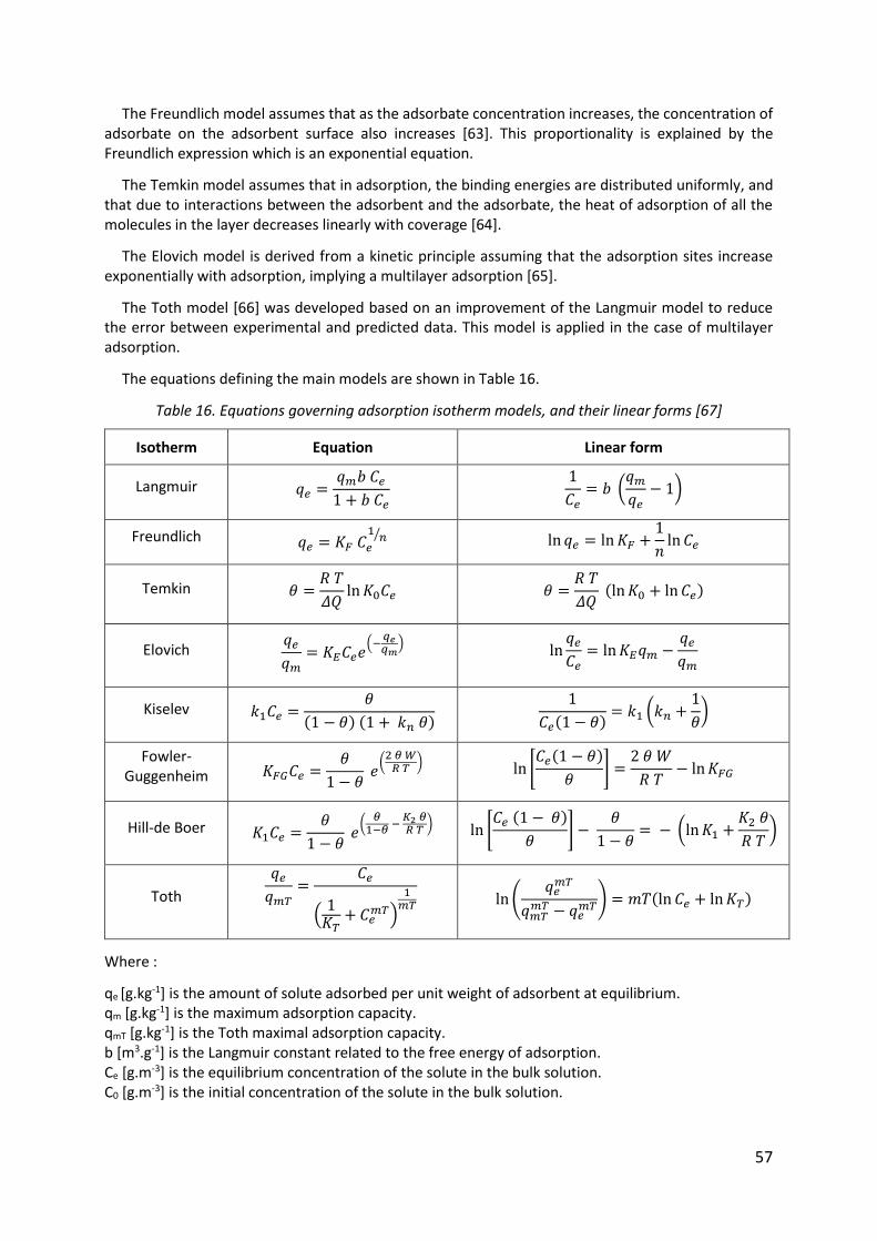
57
The Freundlich model assumes that as the adsorbate concentration increases, the concentration of adsorbate on the adsorbent surface also increases [63]. This proportionality is explained by the Freundlich expression which is an exponential equation.
The Temkin model assumes that in adsorption, the binding energies are distributed uniformly, and that due to interactions between the adsorbent and the adsorbate, the heat of adsorption of all the molecules in the layer decreases linearly with coverage [64].
The Elovich model is derived from a kinetic principle assuming that the adsorption sites increase exponentially with adsorption, implying a multilayer adsorption [65].
The Toth model [66] was developed based on an improvement of the Langmuir model to reduce the error between experimental and predicted data. This model is applied in the case of multilayer adsorption.
The equations defining the main models are shown in Table 16.
Table 16. Equations governing adsorption isotherm models, and their linear forms [67]
Isotherm Equation Linear form
Langmuir 𝑞𝑒 =𝑞𝑚𝑏 𝐶𝑒
1 + 𝑏 𝐶𝑒
1
𝐶𝑒= 𝑏 (
𝑞𝑚
𝑞𝑒− 1)
Freundlich 𝑞𝑒 = 𝐾𝐹 𝐶𝑒
1𝑛⁄
ln 𝑞𝑒 = ln 𝐾𝐹 +1
𝑛ln 𝐶𝑒
Temkin 𝜃 =𝑅 𝑇
𝛥𝑄ln 𝐾0𝐶𝑒 𝜃 =
𝑅 𝑇
𝛥𝑄 (ln 𝐾0 + ln 𝐶𝑒)
Elovich 𝑞𝑒
𝑞𝑚= 𝐾𝐸𝐶𝑒𝑒
(−𝑞𝑒𝑞𝑚
) ln
𝑞𝑒
𝐶𝑒= ln 𝐾𝐸𝑞𝑚 −
𝑞𝑒
𝑞𝑚
Kiselev 𝑘1𝐶𝑒 =𝜃
(1 − 𝜃) (1 + 𝑘𝑛 𝜃)
1
𝐶𝑒(1 − 𝜃)= 𝑘1 (𝑘𝑛 +
1
𝜃)
Fowler-Guggenheim 𝐾𝐹𝐺𝐶𝑒 =
𝜃
1 − 𝜃 𝑒
(2 𝜃 𝑊
𝑅 𝑇) ln [
𝐶𝑒(1 − 𝜃)
𝜃] =
2 𝜃 𝑊
𝑅 𝑇− ln 𝐾𝐹𝐺
Hill-de Boer 𝐾1𝐶𝑒 =𝜃
1 − 𝜃 𝑒
(𝜃
1−𝜃 −
𝐾2 𝜃𝑅 𝑇
) ln [
𝐶𝑒 (1 − 𝜃)
𝜃] −
𝜃
1 − 𝜃= − (ln 𝐾1 +
𝐾2 𝜃
𝑅 𝑇)
Toth
𝑞𝑒
𝑞𝑚𝑇=
𝐶𝑒
(1
𝐾𝑇+ 𝐶𝑒
𝑚𝑇)
1𝑚𝑇
ln (
𝑞𝑒𝑚𝑇
𝑞𝑚𝑇𝑚𝑇 − 𝑞𝑒
𝑚𝑇) = 𝑚𝑇(ln 𝐶𝑒 + ln 𝐾𝑇)
Where :
qe [g.kg-1] is the amount of solute adsorbed per unit weight of adsorbent at equilibrium. qm [g.kg-1] is the maximum adsorption capacity. qmT [g.kg-1] is the Toth maximal adsorption capacity. b [m3.g-1] is the Langmuir constant related to the free energy of adsorption. Ce [g.m-3] is the equilibrium concentration of the solute in the bulk solution. C0 [g.m-3] is the initial concentration of the solute in the bulk solution.
58
KF [g1-(1/n).m(3/n).kg-1] is the Freundlich constant indicative of the relative adsorption capacity of the adsorbent. KT [-] is the Toth equilibrium constant. n [-] is the Freundlich constant indicative of the intensity of the adsorption. mT [-] is the Toth model exponent. θ [-] = qe / qm, is the surface coverage. ΔQ [kJ.mol-1] is the variation of adsorption energy. K0 and K1 [m3.g-1] are the Temkin and Hill-de Boer equilibrium constants respectively. K2 [kJ.mol-1] is the energetic constant of the interaction between adsorbed molecules. KFG [m3.mol-1] is the Fowler-Guggenheim equilibrium constant. W [kJ.mol-1] is the interaction energy between adsorbed molecules.
3.3.5. Adsorption processes
There are two major classes of adsorption processes: the temperature swing adsorption processes (TSA) and the pressure swing adsorption processes (PSA).
Temperature swing adsorption processes
The temperature swing adsorption is the oldest cyclic adsorption process. It consists of two main phases: the adsorption phase and the desorption phase, during which the adsorber is heated. A pre-cooling phase is therefore commonly added to bring the temperature to a level similar to that desired for adsorption.
The main advantage of temperature swing adsorption process compared to pressure swing adsorption is to desorb more easily species strongly adsorbed. For this reason, the temperature swing adsorption processes are used, for example, to capture volatile organic compounds present in many effluents.
Temperature swing adsorption is used whenever the energy required to regenerate a bed is sufficiently large that long high thermal cycles are needed given the strength of the bond between the adsorbate and adsorbent. For example, adsorption of H2O on zeolites.
However, significant time required to heat and cool the adsorber, prevent the use of temperature swing adsorption process in fast cycle. Moreover, the adsorption columns used for temperature swing adsorption cycles are large in size, which has an impact on the cost of the installation. However, unlike pressure swing adsorption processes, that use mechanical energy, temperature swing adsorption processes can use residual heat, which then reduce their operating cost.
Pressure swing adsorption processes
The pressure swing adsorption process was initially introduced as an alternative to temperature swing adsorption process. It is mainly used in separation of some gas species from a mixture of gases, this is another option that complements the traditional separation processes as absorption and cryogenic distillation. In a pressure swing adsorption process, the feed pressure is generally greater than atmospheric pressure. The regeneration pressure may be less than the atmospheric pressure, in this case the process is called vacuum swing adsorption (VSA).
Since the adsorption step is performed at a higher pressure than the pressure of desorption step, intermediate steps are necessary: a compression is required to move from the low to the high pressure at the end of the regeneration step. A decompression step is also necessary to reduce the pressure at the end of the adsorption step. These four steps are the elements of a basic cycle called the Skarstrom cycle. Steps which constitute this cycle, and the variation of the pressure as a function of the different phases, are shown in Fig. 23.

59
Fig. 23: Skarstrom cycle stages and pressure variations [68]
To ensure continuous production, the pressure swing adsorption process must have at least two separation columns. These columns suffer the four steps mentioned above, but with a temporal phase shift leading to a cyclic operation of the pressure swing adsorption process, in which one of the columns is regenerated, while the gas mixture is separated in the other one.
Currently, there are several hundred thousand pressure swing adsorption processes installed worldwide. Their size varies from 6 l.hr-1, often for the production of medical grade oxygen with a purity of 90 % to 2000 m3.h-1 typically for the production of pure hydrogen at 99.999 % [69].
For purification, temperature swing adsorption is generally the process of choice. For bulk separation, pressure swing adsorption is more suitable.
3.4. Membranes technology
A membrane can be defined as a physical barrier for the selective transport of chemical species. As seen in Fig. 24, it allows the restricted passage of one or more constituents. The flux passing through the membrane is called permeate, while the retained is called retentate or concentrate. One or the other of these two flows may be advantageous according to the intended application, and can therefore be used as final product [70].
The driving force in a membrane can be a pressure gradient, a concentration gradient, a temperature gradient, or an electrochemical gradient. Thus, the membranes include a wide variety of materials and structures. Table 17 shows the main materials used by membranes manufacturers.
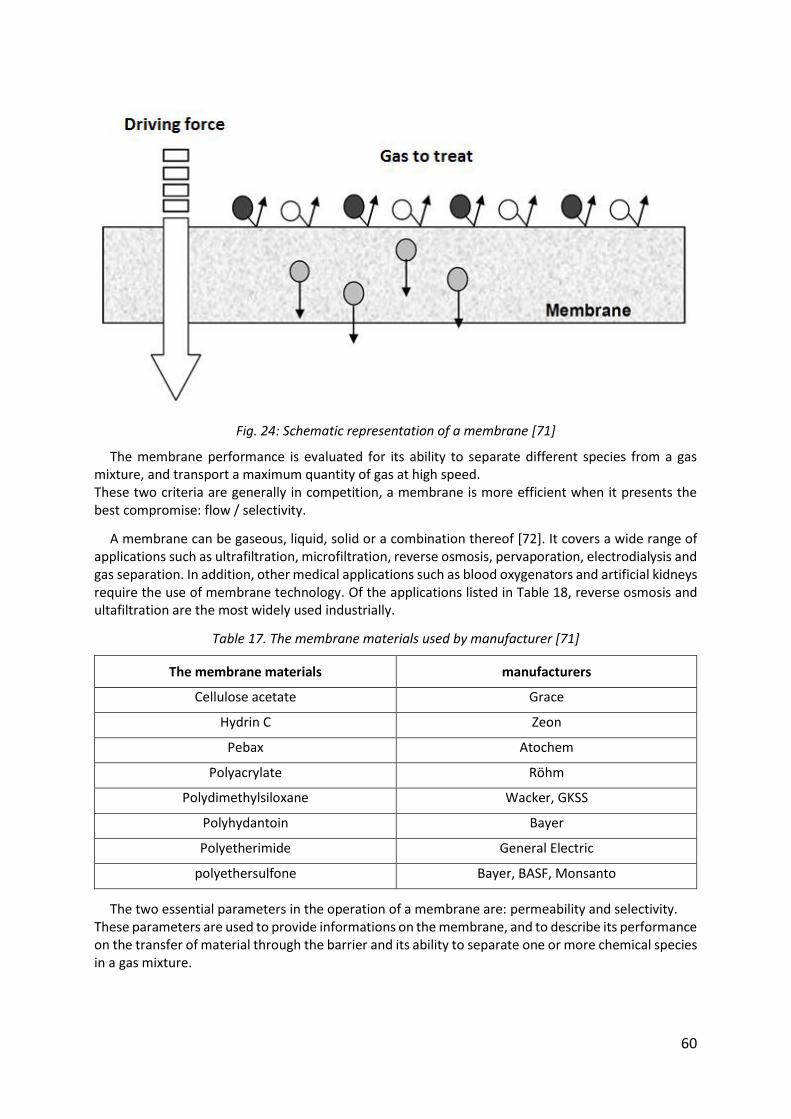
60
Fig. 24: Schematic representation of a membrane [71]
The membrane performance is evaluated for its ability to separate different species from a gas mixture, and transport a maximum quantity of gas at high speed. These two criteria are generally in competition, a membrane is more efficient when it presents the best compromise: flow / selectivity.
A membrane can be gaseous, liquid, solid or a combination thereof [72]. It covers a wide range of applications such as ultrafiltration, microfiltration, reverse osmosis, pervaporation, electrodialysis and gas separation. In addition, other medical applications such as blood oxygenators and artificial kidneys require the use of membrane technology. Of the applications listed in Table 18, reverse osmosis and ultafiltration are the most widely used industrially.
Table 17. The membrane materials used by manufacturer [71]
The membrane materials manufacturers
Cellulose acetate Grace
Hydrin C Zeon
Pebax Atochem
Polyacrylate Röhm
Polydimethylsiloxane Wacker, GKSS
Polyhydantoin Bayer
Polyetherimide General Electric
polyethersulfone Bayer, BASF, Monsanto
The two essential parameters in the operation of a membrane are: permeability and selectivity. These parameters are used to provide informations on the membrane, and to describe its performance on the transfer of material through the barrier and its ability to separate one or more chemical species in a gas mixture.
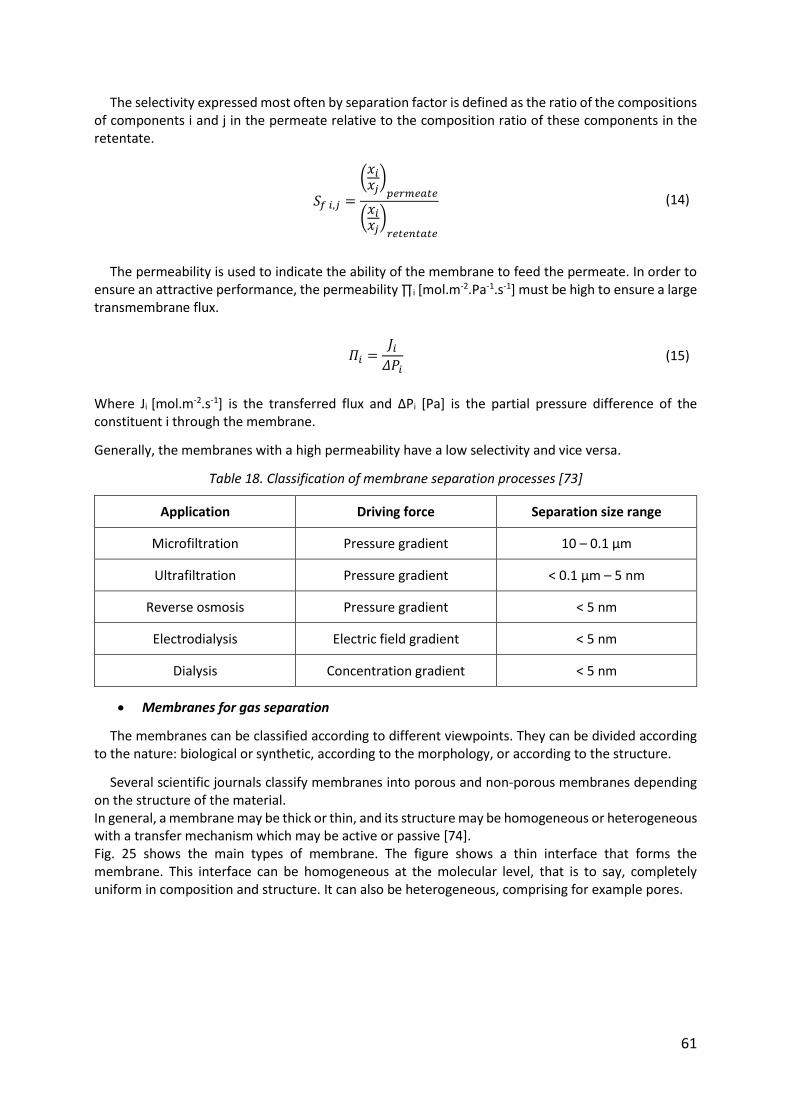
61
The selectivity expressed most often by separation factor is defined as the ratio of the compositions of components i and j in the permeate relative to the composition ratio of these components in the retentate.
𝑆𝑓 𝑖,𝑗 =
(𝑥𝑖𝑥𝑗
)𝑝𝑒𝑟𝑚𝑒𝑎𝑡𝑒
(𝑥𝑖𝑥𝑗
)𝑟𝑒𝑡𝑒𝑛𝑡𝑎𝑡𝑒
(14)
The permeability is used to indicate the ability of the membrane to feed the permeate. In order to ensure an attractive performance, the permeability ∏i [mol.m-2.Pa-1.s-1] must be high to ensure a large transmembrane flux.
𝛱𝑖 =𝐽𝑖
𝛥𝑃𝑖 (15)
Where Ji [mol.m-2.s-1] is the transferred flux and ΔPi [Pa] is the partial pressure difference of the constituent i through the membrane.
Generally, the membranes with a high permeability have a low selectivity and vice versa.
Table 18. Classification of membrane separation processes [73]
Application Driving force Separation size range
Microfiltration Pressure gradient 10 – 0.1 µm
Ultrafiltration Pressure gradient < 0.1 µm – 5 nm
Reverse osmosis Pressure gradient < 5 nm
Electrodialysis Electric field gradient < 5 nm
Dialysis Concentration gradient < 5 nm
Membranes for gas separation
The membranes can be classified according to different viewpoints. They can be divided according to the nature: biological or synthetic, according to the morphology, or according to the structure.
Several scientific journals classify membranes into porous and non-porous membranes depending on the structure of the material. In general, a membrane may be thick or thin, and its structure may be homogeneous or heterogeneous with a transfer mechanism which may be active or passive [74]. Fig. 25 shows the main types of membrane. The figure shows a thin interface that forms the membrane. This interface can be homogeneous at the molecular level, that is to say, completely uniform in composition and structure. It can also be heterogeneous, comprising for example pores.
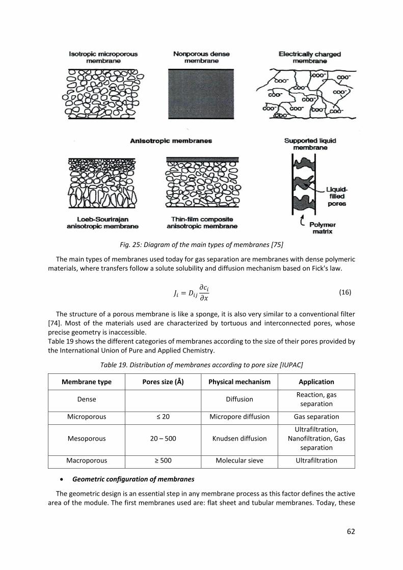
62
Fig. 25: Diagram of the main types of membranes [75]
The main types of membranes used today for gas separation are membranes with dense polymeric materials, where transfers follow a solute solubility and diffusion mechanism based on Fick's law.
𝐽𝑖 = 𝐷𝑖𝑗
𝜕𝑐𝑖
𝜕𝑥 (16)
The structure of a porous membrane is like a sponge, it is also very similar to a conventional filter [74]. Most of the materials used are characterized by tortuous and interconnected pores, whose precise geometry is inaccessible. Table 19 shows the different categories of membranes according to the size of their pores provided by the International Union of Pure and Applied Chemistry.
Table 19. Distribution of membranes according to pore size [IUPAC]
Membrane type Pores size (Å) Physical mechanism Application
Dense Diffusion Reaction, gas
separation
Microporous ≤ 20 Micropore diffusion Gas separation
Mesoporous 20 – 500 Knudsen diffusion Ultrafiltration,
Nanofiltration, Gas separation
Macroporous ≥ 500 Molecular sieve Ultrafiltration
Geometric configuration of membranes
The geometric design is an essential step in any membrane process as this factor defines the active area of the module. The first membranes used are: flat sheet and tubular membranes. Today, these
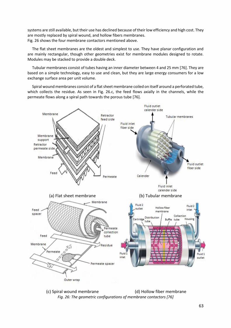
63
systems are still available, but their use has declined because of their low efficiency and high cost. They are mostly replaced by spiral wound, and hollow fibers membranes. Fig. 26 shows the four membrane contactors mentioned above.
The flat sheet membranes are the oldest and simplest to use. They have planar configuration and are mainly rectangular, though other geometries exist for membrane modules designed to rotate. Modules may be stacked to provide a double deck.
Tubular membranes consist of tubes having an inner diameter between 4 and 25 mm [76]. They are based on a simple technology, easy to use and clean, but they are large energy consumers for a low exchange surface area per unit volume.
Spiral wound membranes consist of a flat sheet membrane coiled on itself around a perforated tube, which collects the residue. As seen in Fig. 26.c, the feed flows axially in the channels, while the permeate flows along a spiral path towards the porous tube [76].
(a) Flat sheet membrane (b) Tubular membrane
(c) Spiral wound membrane (d) Hollow fiber membrane
Fig. 26: The geometric configurations of membrane contactors [76]
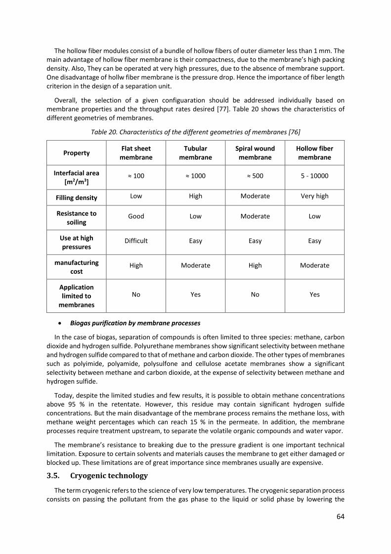
64
The hollow fiber modules consist of a bundle of hollow fibers of outer diameter less than 1 mm. The main advantage of hollow fiber membrane is their compactness, due to the membrane’s high packing density. Also, They can be operated at very high pressures, due to the absence of membrane support. One disadvantage of hollw fiber membrane is the pressure drop. Hence the importance of fiber length criterion in the design of a separation unit.
Overall, the selection of a given configuaration should be addressed individually based on membrane properties and the throughput rates desired [77]. Table 20 shows the characteristics of different geometries of membranes.
Table 20. Characteristics of the different geometries of membranes [76]
Property Flat sheet
membrane Tubular
membrane Spiral wound membrane
Hollow fiber membrane
Interfacial area [m2/m3]
≈ 100 ≈ 1000 ≈ 500 5 - 10000
Filling density Low High Moderate Very high
Resistance to soiling
Good Low Moderate Low
Use at high pressures
Difficult Easy Easy Easy
manufacturing cost
High Moderate High Moderate
Application limited to
membranes
No Yes No Yes
Biogas purification by membrane processes
In the case of biogas, separation of compounds is often limited to three species: methane, carbon dioxide and hydrogen sulfide. Polyurethane membranes show significant selectivity between methane and hydrogen sulfide compared to that of methane and carbon dioxide. The other types of membranes such as polyimide, polyamide, polysulfone and cellulose acetate membranes show a significant selectivity between methane and carbon dioxide, at the expense of selectivity between methane and hydrogen sulfide.
Today, despite the limited studies and few results, it is possible to obtain methane concentrations above 95 % in the retentate. However, this residue may contain significant hydrogen sulfide concentrations. But the main disadvantage of the membrane process remains the methane loss, with methane weight percentages which can reach 15 % in the permeate. In addition, the membrane processes require treatment upstream, to separate the volatile organic compounds and water vapor.
The membrane’s resistance to breaking due to the pressure gradient is one important technical limitation. Exposure to certain solvents and materials causes the membrane to get either damaged or blocked up. These limitations are of great importance since membranes usually are expensive.
3.5. Cryogenic technology
The term cryogenic refers to the science of very low temperatures. The cryogenic separation process consists on passing the pollutant from the gas phase to the liquid or solid phase by lowering the
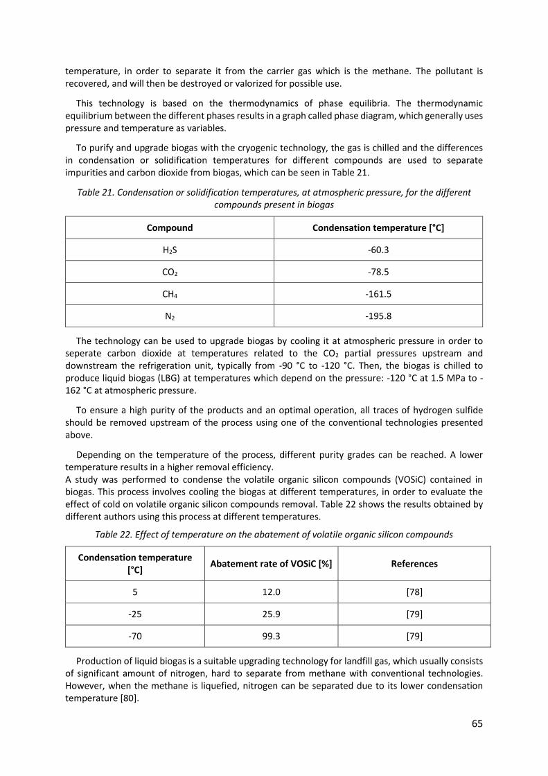
65
temperature, in order to separate it from the carrier gas which is the methane. The pollutant is recovered, and will then be destroyed or valorized for possible use.
This technology is based on the thermodynamics of phase equilibria. The thermodynamic equilibrium between the different phases results in a graph called phase diagram, which generally uses pressure and temperature as variables.
To purify and upgrade biogas with the cryogenic technology, the gas is chilled and the differences in condensation or solidification temperatures for different compounds are used to separate impurities and carbon dioxide from biogas, which can be seen in Table 21.
Table 21. Condensation or solidification temperatures, at atmospheric pressure, for the different compounds present in biogas
Compound Condensation temperature [°C]
H2S -60.3
CO2 -78.5
CH4 -161.5
N2 -195.8
The technology can be used to upgrade biogas by cooling it at atmospheric pressure in order to seperate carbon dioxide at temperatures related to the CO2 partial pressures upstream and downstream the refrigeration unit, typically from -90 °C to -120 °C. Then, the biogas is chilled to produce liquid biogas (LBG) at temperatures which depend on the pressure: -120 °C at 1.5 MPa to -162 °C at atmospheric pressure.
To ensure a high purity of the products and an optimal operation, all traces of hydrogen sulfide should be removed upstream of the process using one of the conventional technologies presented above.
Depending on the temperature of the process, different purity grades can be reached. A lower temperature results in a higher removal efficiency. A study was performed to condense the volatile organic silicon compounds (VOSiC) contained in biogas. This process involves cooling the biogas at different temperatures, in order to evaluate the effect of cold on volatile organic silicon compounds removal. Table 22 shows the results obtained by different authors using this process at different temperatures.
Table 22. Effect of temperature on the abatement of volatile organic silicon compounds
Condensation temperature [°C]
Abatement rate of VOSiC [%] References
5 12.0 [78]
-25 25.9 [79]
-70 99.3 [79]
Production of liquid biogas is a suitable upgrading technology for landfill gas, which usually consists of significant amount of nitrogen, hard to separate from methane with conventional technologies. However, when the methane is liquefied, nitrogen can be separated due to its lower condensation temperature [80].
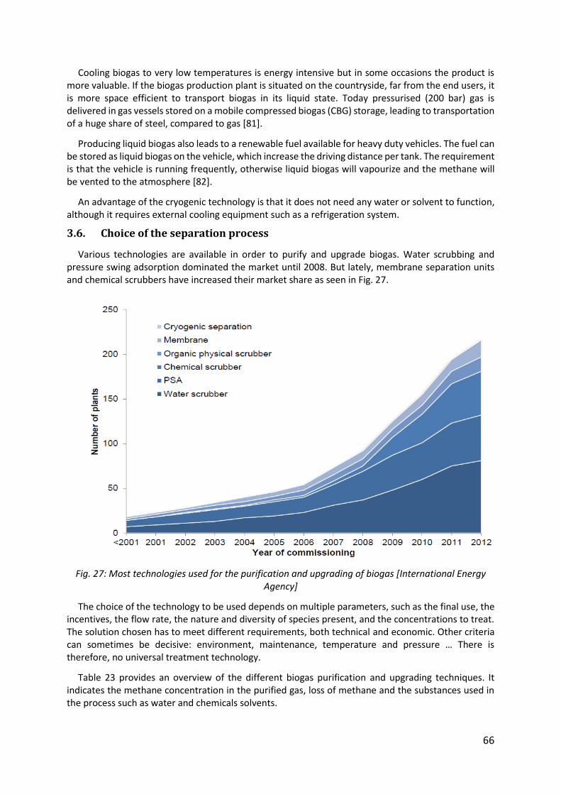
66
Cooling biogas to very low temperatures is energy intensive but in some occasions the product is more valuable. If the biogas production plant is situated on the countryside, far from the end users, it is more space efficient to transport biogas in its liquid state. Today pressurised (200 bar) gas is delivered in gas vessels stored on a mobile compressed biogas (CBG) storage, leading to transportation of a huge share of steel, compared to gas [81].
Producing liquid biogas also leads to a renewable fuel available for heavy duty vehicles. The fuel can be stored as liquid biogas on the vehicle, which increase the driving distance per tank. The requirement is that the vehicle is running frequently, otherwise liquid biogas will vapourize and the methane will be vented to the atmosphere [82].
An advantage of the cryogenic technology is that it does not need any water or solvent to function, although it requires external cooling equipment such as a refrigeration system.
3.6. Choice of the separation process
Various technologies are available in order to purify and upgrade biogas. Water scrubbing and pressure swing adsorption dominated the market until 2008. But lately, membrane separation units and chemical scrubbers have increased their market share as seen in Fig. 27.
Fig. 27: Most technologies used for the purification and upgrading of biogas [International Energy Agency]
The choice of the technology to be used depends on multiple parameters, such as the final use, the incentives, the flow rate, the nature and diversity of species present, and the concentrations to treat. The solution chosen has to meet different requirements, both technical and economic. Other criteria can sometimes be decisive: environment, maintenance, temperature and pressure … There is therefore, no universal treatment technology.
Table 23 provides an overview of the different biogas purification and upgrading techniques. It indicates the methane concentration in the purified gas, loss of methane and the substances used in the process such as water and chemicals solvents.
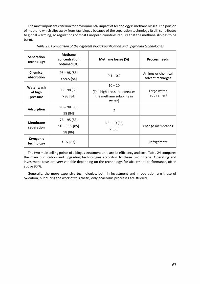
67
The most important criterion for environmental impact of technology is methane losses. The portion of methane which slips away from raw biogas because of the separation technology itself, contributes to global warming, so regulations of most European countries require that the methane slip has to be burnt.
Table 23. Comparison of the different biogas purification and upgrading technologies
Separation
technology
Methane
concentration
obtained [%]
Methane losses [%] Process needs
Chemical
absorption 95 – 98 [83]
> 99.5 [84] 0.1 – 0.2
Amines or chemical solvent recharges
Water wash
at high
pressure
96 – 98 [83]
> 98 [84]
10 – 20
(The high pressure increases the methane solubility in
water)
Large water requirement
Adsorption 95 – 98 [83]
98 [84] 2
Membrane
separation
76 – 95 [83]
90 – 93.5 [85]
98 [86]
6.5 – 10 [85]
2 [86] Change membranes
Cryogenic
technology > 97 [83] Refrigerants
The two main selling points of a biogas treatment unit, are its efficiency and cost. Table 24 compares the main purification and upgrading technologies according to these two criteria. Operating and investment costs are very variable depending on the technology, for abatement performance, often above 90 %.
Generally, the more expensive technologies, both in investment and in operation are those of oxidation, but during the work of this thesis, only anaerobic processes are studied.

68
Table 24. Performances, costs, advantages and disadvantages of separation processes [87]
Separation technology
Efficiency [%]
Investment cost
[€/m3.h-1]
Operating cost
[€/1000 m3]
Advantages Disadvantages
Absorption 95 – 98 7 – 32 1.7 – 8.2
- Simple operation for a wide range of flow rates, concentrations and compounds.
- Possible pollutant recovery.
- High operating costs, related to the liquid phase in general.
- Generating a polluted aqueous effluent.
- Can generate additional separation operations.
Adsorption on
activated carbon
80 – 90 7 – 55 0.7 – 2.4
- Very easy to use.
- Tolerates flow variations.
- Possible pollutant recovery.
- Add an operating cost, associated with the regeneration of
the adsorbent.
Condensation
50 – 90 5 – 37 1.4 – 8.2 - Possible pollutant
recovery. - Icing Possibility
The investment costs of the different technologies do not differ greatly, especially at high flow rates. They are presented in Fig. 28.

69
Fig. 28: Comparison of investment costs of different biogas purification and upgrading technologies [88]
Separation technologies: (__Δ__) Chemical absorption (Amines) ; (- -□- -) Water wash ; (- .○- .) Membranes ; (…+…)
Adsorption (PSA)
Chemical absorption using amines as chemical solvent is slightly more expensive in terms of investment, and membrane separation process is less costly for low flow rates. This investment cost criterion begins to converge for all technologies at higher flow rates.
3.7. Conclusion
This chapter has introduced the various technologies used for the purification and upgrading of biogas. These separation methods were compared according to several criteria such as separation efficiency, the environmental impact and investment and operating costs.
The work of this thesis is part of the project led by the company Cryo Pur®, which aims to create an innovative biogas cryogenic purification and upgrading process for the production of a renewable fuel and liquid carbon dioxide.
For carbon dioxide capture, Cryo Pur® company has developed a new technology which consists of anti-sublimating the carbon dioxide on a low temperature surface (from -90 °C to -120 °C), thus transforming CO2 directly from its gaseous phase into a solid phase frosted on the cold surface [89]. Having regard to the need to liquefy the biogas at low temperatures to be used as vehicle fuel, the best alternative to the conventional technologies is therefore to upgrade biogas with cryogenic technology.
Biogas upgrading depends on the concentrations of hydrogen sulfide present. Indeed, this compound must be completely eliminated upstream of the process to ensure high quality products and to prevent corrosion of equipment such as heat exchangers used in the cryogenic process. Hence the need to use a process with a very high efficiency, to be able to eliminate all the hydrogen sulfide present in the biogas. On the whole, the lowest methane losses are indicated for chemical absorption and adsorption processes, and the highest one relates to membranes and water wash.
0
1000
2000
3000
4000
5000
6000
7000
0 500 1000 1500 2000 2500
Inve
stm
en
t co
st [€
/Nm
3.h
-1]
Biogas flow rate [Nm3.h-1]

70
Finally, the choice was focused on the following two technologies used for the removal of hydrogen sulfide:
Chemical absorption in a structured packed column using sodium hydroxide (NaOH) as solvent.
Adsorption in a fixed bed using activated carbon.
The next chapter will present the technology developed by Cryo Pur® Company for purification and upgrading of biogas.
71
Chapter 4: Industrial demonstrator description Résumé :
Ce chapitre présente le procédé industriel dans lequel se situe l’étape de désulfurisation étudiée. Il s’agit d’un démonstrateur industriel appelé « BioGNVAL » développé par la société Cryo Pur® en partenariat avec SUEZ et l’Agence De l’Environnement et de la Maitrise de l’Energie (ADEME). GNVert et IVECO sont également partenaires du projet BioGNVAL.
Ce pilote traite 85 Nm3/h de biogaz issu de la station d’épuration du Syndicat Interdépartemental pour l’Assainissement de l’Agglomération Parisienne (SIAAP) à Valenton, la deuxième plus grande en France.
Une des voies de valorisation du biogaz est la production de bio-GNL (GNL : Gaz Naturel liquéfié) qui se présente comme un carburant neutre en émissions de gaz à effet de serre avec plusieurs avantages économiques et environnementaux. La production de ce type de carburant requiert de très basses températures afin de liquéfier le bio-méthane, ce qui peut induire la solidification des impuretés et donc des problèmes de fonctionnement des installations. Ces impuretés doivent donc être séparées du biogaz, en particulier l’élimination de l’hydrogène sulfuré est impérative afin de garantir un fonctionnement optimal et une grande pureté des autres composés à valoriser comme le dioxyde de carbone. De surcroît, la présence de H2S dans le biogaz est une source de corrosion pour les équipements comme les pompes et les échangeurs de chaleur.

72
4.1. Introduction
Experiments were performed on the industrial demonstrator “BioGNVAL” treating 85 Nm3/h of
biogas from the Valenton water treatment plant, the second biggest in France run by the SIAAP (Public
society serving the Paris region). The demonstrator shown in Fig. 29 was developed by the Cryo Pur®
Company. It was built in partnership with SUEZ as part of the BioGNVAL project, and partially funded
by the ‘Invest in the Future’ program run by the ADEME (French Environment and Energy Management
Agency). GNVert (Engie) and IVECO are also partners in the BioGNVal project, providing the Bio-LNG
distribution station and the heavy goods vehicle Flex Fuel gas / Bio-LNG respectively.
Fig. 29: BioGNVAL demonstrator located at Valenton water treatment plant [9]
The BioGNVAL pilot plant uses a cryogenic method to purify and liquefy biogas efficiently without
loss of methane and without emitting greenhouse gases. The system generates two products from
biogas: liquid bio-methane and bioCO2 at purity level greater than 99.995 % respecting EIGA (European
Industrial Gases Association) specifications [90].
The general principle of operation of the BioGNVAL pilot plant is depicted in Fig. 30. It takes place
in three main stages:
Pretreatment or purification which is to remove trace compounds present in the biogas as
hydrogen sulfide, water vapor and siloxanes.
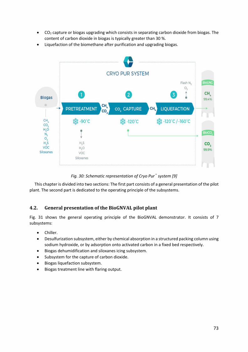
73
CO2 capture or biogas upgrading which consists in separating carbon dioxide from biogas. The
content of carbon dioxide in biogas is typically greater than 30 %.
Liquefaction of the biomethane after purification and upgrading biogas.
Fig. 30: Schematic representation of Cryo Pur® system [9]
This chapter is divided into two sections: The first part consists of a general presentation of the pilot
plant. The second part is dedicated to the operating principle of the subsystems.
4.2. General presentation of the BioGNVAL pilot plant
Fig. 31 shows the general operating principle of the BioGNVAL demonstrator. It consists of 7
subsystems:
Chiller.
Desulfurization subsystem, either by chemical absorption in a structured packing column using
sodium hydroxide, or by adsorption onto activated carbon in a fixed bed respectively.
Biogas dehumidification and siloxanes icing subsystem.
Subsystem for the capture of carbon dioxide.
Biogas liquefaction subsystem.
Biogas treatment line with flaring output.
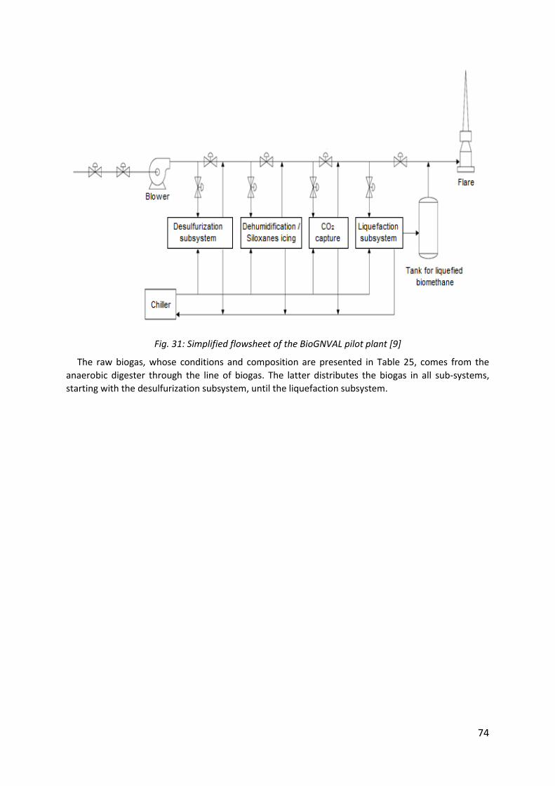
74
Fig. 31: Simplified flowsheet of the BioGNVAL pilot plant [9]
The raw biogas, whose conditions and composition are presented in Table 25, comes from the
anaerobic digester through the line of biogas. The latter distributes the biogas in all sub-systems,
starting with the desulfurization subsystem, until the liquefaction subsystem.
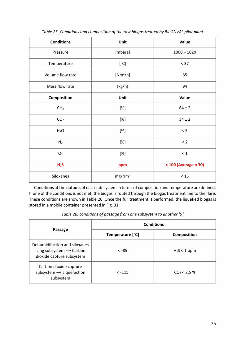
75
Table 25. Conditions and composition of the raw biogas treated by BioGNVAL pilot plant
Conditions Unit Value
Pressure [mbara] 1000 – 1020
Temperature [°C] < 37
Volume flow rate [Nm3/h] 85
Mass flow rate [kg/h] 94
Composition Unit Value
CH4 [%] 64 ± 2
CO2 [%] 34 ± 2
H2O [%] < 5
N2 [%] < 2
O2 [%] < 1
H2S ppm < 100 (Average ≈ 30)
Siloxanes mg/Nm3 < 15
Conditions at the outputs of each sub-system in terms of composition and temperature are defined.
If one of the conditions is not met, the biogas is routed through the biogas treatment line to the flare.
These conditions are shown in Table 26. Once the full treatment is performed, the liquefied biogas is
stored in a mobile container presented in Fig. 31.
Table 26. conditions of passage from one subsystem to another [9]
Passage Conditions
Temperature [°C] Composition
Dehumidifaction and siloxanes
icing subsystem ⟶ Carbon
dioxide capture subsystem
< -85 H2S < 1 ppm
Carbon dioxide capture
subsystem ⟶ Liquefaction
subsystem
< -115 CO2 < 2.5 %
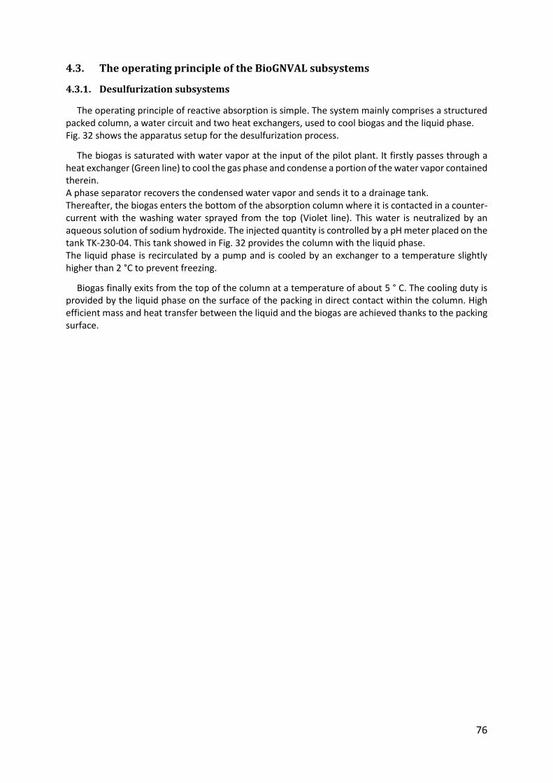
76
4.3. The operating principle of the BioGNVAL subsystems
4.3.1. Desulfurization subsystems
The operating principle of reactive absorption is simple. The system mainly comprises a structured packed column, a water circuit and two heat exchangers, used to cool biogas and the liquid phase. Fig. 32 shows the apparatus setup for the desulfurization process.
The biogas is saturated with water vapor at the input of the pilot plant. It firstly passes through a heat exchanger (Green line) to cool the gas phase and condense a portion of the water vapor contained therein. A phase separator recovers the condensed water vapor and sends it to a drainage tank. Thereafter, the biogas enters the bottom of the absorption column where it is contacted in a counter-current with the washing water sprayed from the top (Violet line). This water is neutralized by an aqueous solution of sodium hydroxide. The injected quantity is controlled by a pH meter placed on the tank TK-230-04. This tank showed in Fig. 32 provides the column with the liquid phase. The liquid phase is recirculated by a pump and is cooled by an exchanger to a temperature slightly higher than 2 °C to prevent freezing.
Biogas finally exits from the top of the column at a temperature of about 5 ° C. The cooling duty is provided by the liquid phase on the surface of the packing in direct contact within the column. High efficient mass and heat transfer between the liquid and the biogas are achieved thanks to the packing surface.
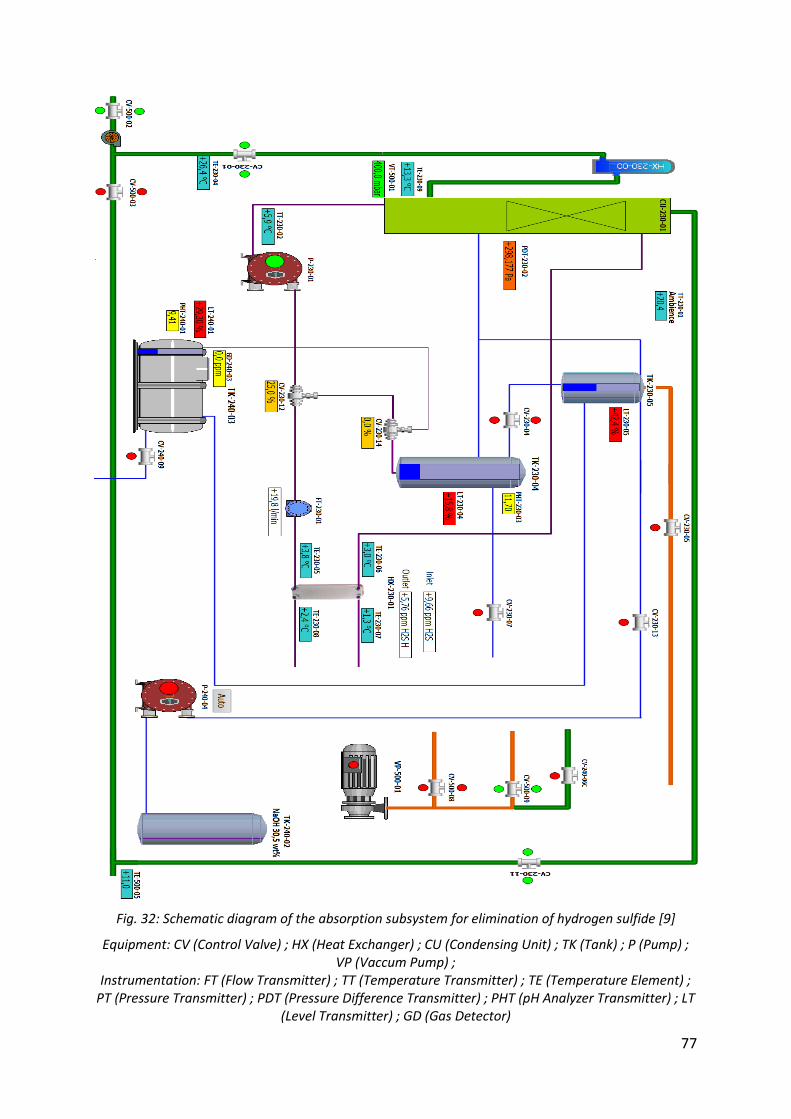
77
Fig. 32: Schematic diagram of the absorption subsystem for elimination of hydrogen sulfide [9]
Equipment: CV (Control Valve) ; HX (Heat Exchanger) ; CU (Condensing Unit) ; TK (Tank) ; P (Pump) ; VP (Vaccum Pump) ;
Instrumentation: FT (Flow Transmitter) ; TT (Temperature Transmitter) ; TE (Temperature Element) ; PT (Pressure Transmitter) ; PDT (Pressure Difference Transmitter) ; PHT (pH Analyzer Transmitter) ; LT
(Level Transmitter) ; GD (Gas Detector)
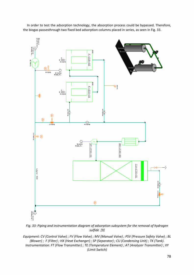
78
In order to test the adsorption technology, the absorption process could be bypassed. Therefore,
the biogas passesthrough two fixed bed adsorption columns placed in series, as seen in Fig. 33.
Fig. 33: Piping and instrumentation diagram of adsorption subsystem for the removal of hydrogen sulfide [9]
Equipment: CV (Control Valve) ; FV (Flow Valve) ; MV (Manual Valve) ; PSV (Pressure Safety Valve) ; BL (Blower) ; F (Filter) ; HX (Heat Exchanger) ; SP (Separator) ; CU (Condensing Unit) ; TK (Tank).
Instrumentation: FT (Flow Transmitter) ; TE (Temperature Element) ; AT (Analyzer Transmitter) ; XY (Limit Switch)
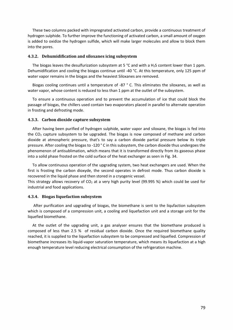
79
These two columns packed with impregnated activated carbon, provide a continuous treatment of
hydrogen sulphide. To further improve the functioning of activated carbon, a small amount of oxygen
is added to oxidize the hydrogen sulfide, which will make larger molecules and allow to block them
into the pores.
4.3.2. Dehumidification and siloxanes icing subsystem
The biogas leaves the desulfurization subsystem at 5 °C and with a H2S content lower than 1 ppm.
Dehumidification and cooling the biogas continue until -40 °C. At this temperature, only 125 ppm of
water vapor remains in the biogas and the heaviest Siloxanes are removed.
Biogas cooling continues until a temperature of -87 ° C. This eliminates the siloxanes, as well as
water vapor, whose content is reduced to less than 1 ppm at the outlet of the subsystem.
To ensure a continuous operation and to prevent the accumulation of ice that could block the
passage of biogas, the chillers used contain two evaporators placed in parallel to alternate operation
in frosting and defrosting mode.
4.3.3. Carbon dioxide capture subsystem
After having been purified of hydrogen sulphide, water vapor and siloxane, the biogas is fed into
the CO2 capture subsystem to be upgraded. The biogas is now composed of methane and carbon
dioxide at atmospheric pressure, that's to say a carbon dioxide partial pressure below its triple
pressure. After cooling the biogas to -120 ° C in this subsystem, the carbon dioxide thus undergoes the
phenomenon of antisublimation, which means that it is transformed directly from its gaseous phase
into a solid phase frosted on the cold surface of the heat exchanger as seen in Fig. 34.
To allow continuous operation of the upgrading system, two heat exchangers are used. When the
first is frosting the carbon dioxyde, the second operates in defrost mode. Thus carbon dioxide is
recovered in the liquid phase and then stored in a cryogenic vessel.
This strategy allows recovery of CO2 at a very high purity level (99.995 %) which could be used for
industrial and food applications.
4.3.4. Biogas liquefaction subsystem
After purification and upgrading of biogas, the biomethane is sent to the liqufaction subsystem
which is composed of a compression unit, a cooling and liquefaction unit and a storage unit for the
liquefied biomethane.
At the outlet of the upgrading unit, a gas analyser ensures that the biomethane produced is
composed of less than 2.5 % of residual carbon dioxide. Once the required biomethane quality
reached, it is supplied to the liquefaction subsystem to be compressed and liquefied. Compression of
biomethane increases its liquid-vapor saturation temperature, which means its liquefaction at a high
enough temperature level reducing electrical consumption of the refrigeration machine.
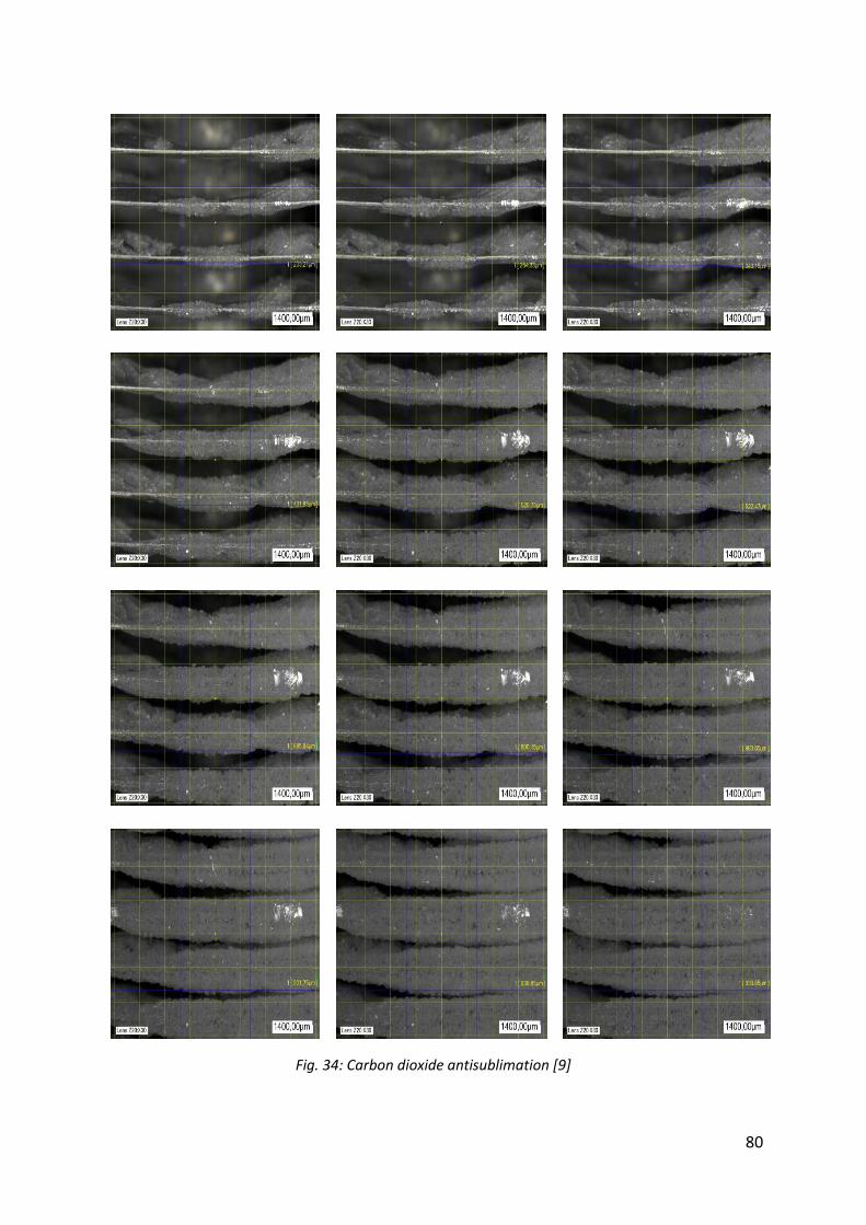
80
Fig. 34: Carbon dioxide antisublimation [9]
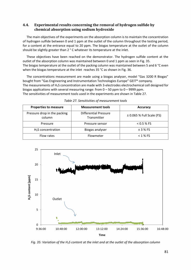
81
4.4. Experimental results concerning the removal of hydrogen sulfide by chemical absorption using sodium hydroxide
The main objectives of the experiments on the absorption column is to maintain the concentration of hydrogen sulfide between 0 and 1 ppm at the outlet of the column throughout the testing period, for a content at the entrance equal to 20 ppm. The biogas temperature at the outlet of the column should be slightly greater than 2 ° C whatever its temperature at the inlet.
These objectives have been reached on the demonstrator. The hydrogen sulfide content at the outlet of the absorption column was maintained between 0 and 1 ppm as seen in Fig. 35. The biogas temperature at the outlet of the packing column was maintained between 5 and 6 °C even when the biogas temperature at the inlet reaches 35 °C as shown in Fig. 36.
The concentrations measurement are made using a biogas analyser, model “Gas 3200 R Biogas” bought from “Gas Engineering and Instrumentation Technologies Europe” GEIT® company. The measurements of H2S concentration are made with 3-electrodes electrochemical cell designed for biogas applications with several measuring range: from 0 – 50 ppm to 0 – 9999 ppm. The sensitivities of measurement tools used in the experiments are shown in Table 27.
Table 27. Sensitivities of measurement tools
Properties to measure Measurement tools Accuracy
Pressure drop in the packing column
Differential Pressure Transmitter
± 0.065 % Full Scale (FS)
Pressure Pressure sensor < 0.5 % FS
H2S concentration Biogas analyser ± 3 % FS
Flow rates Flowmeter < 1 % FS
Fig. 35: Variation of the H2S content at the inlet and at the outlet of the absorption column
0
5
10
15
20
25
9:36:00 10:48:00 12:00:00 13:12:00 14:24:00 15:36:00 16:48:00
H2S
co
nte
nt
[pp
m]
Time
Inlet
Outlet
82
Fig. 36: Variation of the biogas temperature at the inlet of the demonstrator and at the outlet of the
absorption column
Sodium hydroxide was used as chemical solvant for the removal of hydrogen sulfide. The weight percentage of NaOH in water is equal to 30.5 wt%. Averaged over all experiments, sodium hydroxide consumption was assessed at 6 l/h (solution containing 30.5 wt% of NaOH and 69.5 wt% of H2O). This consumption was calculated with an indicator allowing the NaOH level measurement in the tank TK-240-02 (See Fig. 32). This consumption is very excessive relative to the theoretical consumption of 1.35 l/hr of commercial caustic soda.
This overconsumption is explained by desorption of hydrogen sulfide, because the reaction between hydrogen sulphide and sodium hydroxide is reversible (R.11). It leads to the formation of sodium sulfide (Na2S) that is unstable in water.
Fig. 37 shows the desorption phenomenon observed during experiments. Indeed, stopping the injection of sodium hydroxide at 13:45:00 (See Fig. 37) shows that the hydrogen sulfide content at the outlet of the column is greater than its content at the inlet. This explains the overconsumption of the solvent.
0
5
10
15
20
25
30
35
40
7:12:00 8:24:00 9:36:00 10:48:00 12:00:00 13:12:00 14:24:00 15:36:00 16:48:00
Bio
gas
tem
pe
ratu
re [
°C]
Time
Inlet
Outlet
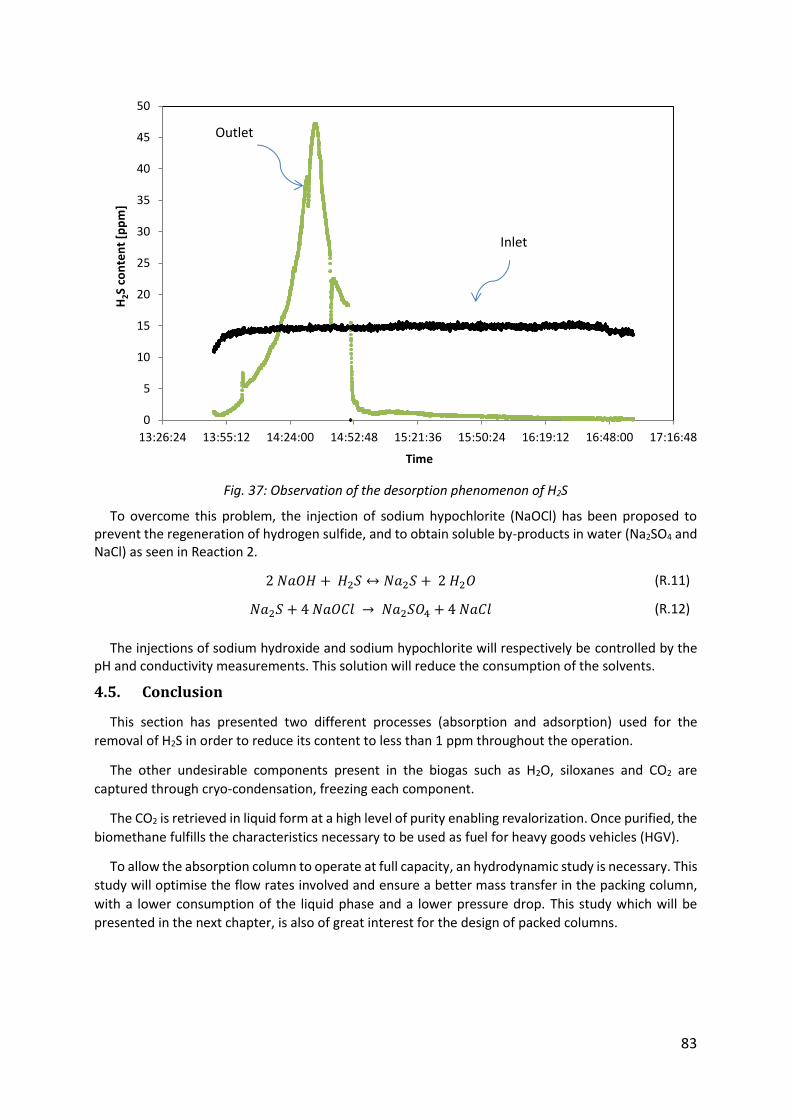
83
Fig. 37: Observation of the desorption phenomenon of H2S
To overcome this problem, the injection of sodium hypochlorite (NaOCl) has been proposed to prevent the regeneration of hydrogen sulfide, and to obtain soluble by-products in water (Na2SO4 and NaCl) as seen in Reaction 2.
2 𝑁𝑎𝑂𝐻 + 𝐻2𝑆 ↔ 𝑁𝑎2𝑆 + 2 𝐻2𝑂 (R.11)
𝑁𝑎2𝑆 + 4 𝑁𝑎𝑂𝐶𝑙 → 𝑁𝑎2𝑆𝑂4 + 4 𝑁𝑎𝐶𝑙 (R.12)
The injections of sodium hydroxide and sodium hypochlorite will respectively be controlled by the pH and conductivity measurements. This solution will reduce the consumption of the solvents.
4.5. Conclusion
This section has presented two different processes (absorption and adsorption) used for the
removal of H2S in order to reduce its content to less than 1 ppm throughout the operation.
The other undesirable components present in the biogas such as H2O, siloxanes and CO2 are
captured through cryo-condensation, freezing each component.
The CO2 is retrieved in liquid form at a high level of purity enabling revalorization. Once purified, the
biomethane fulfills the characteristics necessary to be used as fuel for heavy goods vehicles (HGV).
To allow the absorption column to operate at full capacity, an hydrodynamic study is necessary. This
study will optimise the flow rates involved and ensure a better mass transfer in the packing column,
with a lower consumption of the liquid phase and a lower pressure drop. This study which will be
presented in the next chapter, is also of great interest for the design of packed columns.
0
5
10
15
20
25
30
35
40
45
50
13:26:24 13:55:12 14:24:00 14:52:48 15:21:36 15:50:24 16:19:12 16:48:00 17:16:48
H2S
con
ten
t [p
pm
]
Time
Inlet
Outlet
84
Chapter 5: Hydrodynamic study of gas-liquid countercurrent flows in structured packing columns
Résumé :
Ce chapitre compare trois modèles existants utilisés pour la prédiction des paramètres
hydrodynamiques dans des colonnes à garnissage structuré.
Ces modèles sont utilisés pour évaluer la perte de pression, la rétention liquide, l’aire interfaciale
effective, les coefficients de transfert de masse et les points de transition. Les résultats de ces modèles
sont comparés à des données expérimentales afin de choisir celui avec le meilleur ajustement.
Les comparaisons ont été effectuées en utilisant deux systèmes : Air - Eau et Air - Kerosol 200 et un
garnissage structuré de type Flexipac 350Y.
Le modèle choisi est basé sur des corrélations semi-empiriques contenant des constantes et des
exposants définis selon des mesures expérimentales. Pour rendre le modèle plus représentatif du
système d'intérêt (biogaz contenant du H2S / solution aqueuse d’hydroxyde de sodium), ces constantes
ont été modifiées et certains exposants ont été ajustés en fonction de la vitesse superficielle du liquide
et la densité.
Une fois le modèle modifié, les résultats de la perte de pression ont été comparés aux données
expérimentales obtenues sur le démonstrateur BioGNVAL. Les résultats obtenus sont en bon accord
mais il est judicieux de noter que ce modèle peut perdre de sa précision en variant les applications.
Par conséquent, ce modèle est idéal pour prédire avec précision les trois régions opérationnelles
d'une colonne à garnissage structuré à petite échelle utilisée pour des applications de biogaz ou de gaz
naturel.

85
5.1. Introduction
Today, in modern absorption columns, structured packings are widely used, thanks to their higher capacity and lower pressure drop compared to random packings. Structured packings were used for the first time in 1950 [91]. They are in continuous development to expand their use and improve their efficiency. They provide a large surface area for the liquid and gas phases to be in direct contact within the column. High efficient mass transfer between the two phases is achieved thanks to the packing surface.
This work compares three existing models used for the prediction of hydrodynamic parameters in structured packing columns. These models are used to evaluate pressure drop, liquid holdup, effective interfacial area, mass transfer coefficients and transition points. The results obtained with these models are compared to experimental data in order to choose the one with the best fit. Comparisons were made using Flexipac 350Y structured packing and two systems: Air – Water and Air – Kerosol 200. The model chosen is based on semi-empirical correlations using constants and exponents defined according to experimental measurements. To adapt the model to biogas application and to make it more representative of the system of interest, these constants were optimized and some exponents have been adjusted. Once the model modified, the results of pressure drop were compared to data from BioGNVAL pilot plant.
5.2. Theoretical principles
In a packed column, hydrodynamics and mass transfer processes occur simultaneously. They are correlated and the link parameter is liquid holdup hL defined as the volume of the liquid per unit volume of the column. Equation (17) defined by Chan and Fair [92] for sieve trays illustrated the relation between the two processes.
𝑘𝑉𝑎𝑒 = 316 𝐷𝑉
0,5 (1030 𝑓 + 867 𝑓2)
ℎ𝐿0,5 (17)
Regarding the hydrodynamic analysis, increasing the velocity of liquid and gas, results in an increase of the liquid holdup and the thickness of the liquid film which leads to an increase in pressure drop.
About mass transfer analysis, increasing liquid holdup causes the enlargement of the interfacial area leading to higher mass transfer rates.
The curve which represents the evolution of the pressure drop or the liquid holdup as a function of the gas capacity factor Fc is divided by two points (loading and flooding points) into three operating regions as seen in Fig. 38.
The liquid flow rate is not influenced by the counter-current flow of the gas in the preloading region, as can be seen in Fig. 38.b which presents the evolution of the liquid holdup as a function of the gas capacity factor defined by Equation (18).
𝐹𝑐 = 𝑢𝑉 × √𝜌𝑉 (18)
The loading point represented by the line AA in Fig. 38 is reached when the slope of the liquid holdup curve starts to increase, or when the wet pressure drop curve starts to deviate from the pressure drop in a dry column. The flooding point is represented by the line BB in Fig. 38. It is the point where the slope of pressure drop and liquid holdup curves tends toward infinity. Therefore, it is necessary to predict accurately the transition points because they characterize the capacity of a packing column. According to Paquet [93], under-predicting the flooding point will prevent the column to operate at its optimal conditions, and its capacity could be very low. However, over-predicting the flooding point may lead to higher pressure drop which could be problematic.

86
Because of the lack of predictive models, and because of the imprecision of existing ones to accurately predict the hydrodynamic parameters for some specific applications such as biogas purification, most distillation and packing columns are still being designed based on experimental data from a pilot plant [94].
The objective of this work is to find a model adapted for the representation of the experimental results obtained on the BioGNVAL pilot plant. To this aim, three literature models for the hydrodynamics in structured packing columns have been compared: Billet and Schultes model [95], SRP model [96] and Delft model [97]. These models have been developed on dimensionless analysis and experimental data obtained using a distillation column. The two first models are implemented in the process simulator Aspen Plus®. The three models are described in detail in the following section.
Fig. 38.a: Pressure drop evolution in a packing column
Fig. 38.b: Liquid holdup evolution in a packing column
(__Δ__) Dry bed ; (- -□- -) 1 ; (- .○- .) 2 ; (…Δ…) 3 (AA) Loading point ; (BB) Flooding point
Liquid load: 1 < 2 < 3
(__Δ__) 1 ; (- -□- -) 2 ; (- .○- .) 3 ; (…Δ…) 4 (AA) Loading point ; (BB) Flooding point
Liquid load: 1 < 2 < 3 < 4
5.2.1. Billet and Schultes model
The Billet and Schultes model [95] was at the base founded for random packings. Then, it was extended to cover structured packings. Based on semi-empirical correlations, this model assumes that the packing void fraction is represented by vertical tubes where the liquid is sprayed from the top as a film that meets the gas flow in a counter-current configuration. The angle between the corrugations of the packing is not taken into account by the Billet and Schultes model.
Pre
ssu
re d
rop
[P
a/m
]
Gas capacity factor [(m/s).(kg/m3)0.5]
B
B
A
A
Liq
uid
ho
ldu
p [
m3/m
3]
Gas capacity factor [(m/s).(kg/m3)0.5]
A
A
B
B
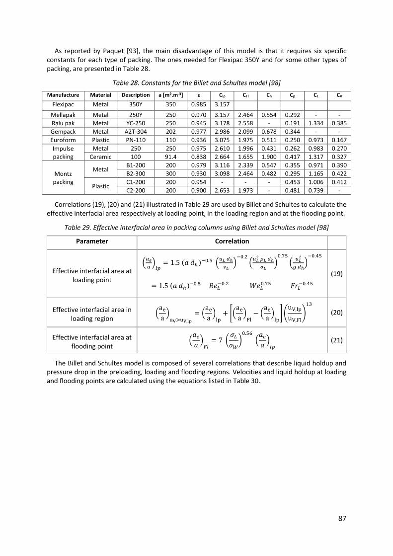
87
As reported by Paquet [93], the main disadvantage of this model is that it requires six specific constants for each type of packing. The ones needed for Flexipac 350Y and for some other types of packing, are presented in Table 28.
Table 28. Constants for the Billet and Schultes model [98]
Manufacture Material Description a [m2.m-3] ε Clp CFl Ch Cp CL CV
Flexipac Metal 350Y 350 0.985 3.157
Mellapak Metal 250Y 250 0.970 3.157 2.464 0.554 0.292 - -
Ralu pak Metal YC-250 250 0.945 3.178 2.558 - 0.191 1.334 0.385
Gempack Metal A2T-304 202 0.977 2.986 2.099 0.678 0.344 - -
Euroform Plastic PN-110 110 0.936 3.075 1.975 0.511 0.250 0.973 0.167
Impulse packing
Metal 250 250 0.975 2.610 1.996 0.431 0.262 0.983 0.270
Ceramic 100 91.4 0.838 2.664 1.655 1.900 0.417 1.317 0.327
Montz packing
Metal B1-200 200 0.979 3.116 2.339 0.547 0.355 0.971 0.390
B2-300 300 0.930 3.098 2.464 0.482 0.295 1.165 0.422
Plastic C1-200 200 0.954 - - - 0.453 1.006 0.412
C2-200 200 0.900 2.653 1.973 - 0.481 0.739 -
Correlations (19), (20) and (21) illustrated in Table 29 are used by Billet and Schultes to calculate the effective interfacial area respectively at loading point, in the loading region and at the flooding point.
Table 29. Effective interfacial area in packing columns using Billet and Schultes model [98]
Parameter Correlation
Effective interfacial area at loading point
(𝑎𝑒
𝑎)
𝑙𝑝= 1.5 (𝑎 𝑑ℎ)−0.5 (
𝑢𝐿 𝑑ℎ
𝜈𝐿)
−0.2(
𝑢𝐿2 𝜌𝐿 𝑑ℎ
𝜎𝐿)
0.75
(𝑢𝐿
2
𝑔 𝑑ℎ)
−0.45
= 1.5 (𝑎 𝑑ℎ)−0.5 𝑅𝑒𝐿
−0.2 𝑊𝑒𝐿0.75 𝐹𝑟𝐿
−0.45
(19)
Effective interfacial area in loading region
(ae
a)
uV>uV,lp
= (ae
a)
lp+ [(
ae
a)
Fl− (
ae
a)
lp] (
uV,lp
uV,Fl)
13
(20)
Effective interfacial area at flooding point
(𝑎𝑒
𝑎)
𝐹𝑙= 7 (
𝜎𝐿
𝜎𝑊)
0.56
(𝑎𝑒
𝑎)
𝑙𝑝 (21)
The Billet and Schultes model is composed of several correlations that describe liquid holdup and pressure drop in the preloading, loading and flooding regions. Velocities and liquid holdup at loading and flooding points are calculated using the equations listed in Table 30.
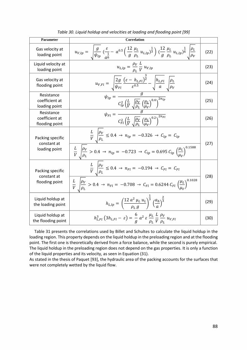
88
Table 30. Liquid holdup and velocities at loading and flooding point [99]
Parameter Correlation
Gas velocity at loading point
𝑢𝑉,𝑙𝑝 = √𝑔
𝜓𝑙𝑝 (
휀
𝑎16
− 𝑎0.5 ( 12
𝑔 𝜇𝐿
𝜌𝐿 𝑢𝐿,𝑙𝑝)
13 ) (
12
𝑔 𝜇𝐿
𝜌𝐿 𝑢𝐿,𝑙𝑝)
16 √
𝜌𝐿
𝜌𝑉 (22)
Liquid velocity at loading point
𝑢𝐿,𝑙𝑝 = 𝜌𝑉
𝜌𝐿 𝐿
𝑉 𝑢𝑉,𝑙𝑝 (23)
Gas velocity at flooding point 𝑢𝑉,𝐹𝑙 = √
2𝑔
𝜓𝐹𝑙 (휀 − ℎ𝐿,𝐹𝑙)
32
휀0.5− √
ℎ𝐿,𝐹𝑙
𝑎 √
𝜌𝐿
𝜌𝑉 (24)
Resistance coefficient at loading point
𝜓𝑙𝑝 = 𝑔
𝐶𝑙𝑝2 (
𝐿𝑉
√𝜌𝑉𝜌𝐿
(𝜇𝐿𝜇𝑉
)0.4
)2𝑛𝑙𝑝
(25)
Resistance coefficient at flooding point
𝜓𝐹𝑙 = 𝑔
𝐶𝐹𝑙2 (
𝐿𝑉
√𝜌𝑉𝜌𝐿
(𝜇𝐿𝜇𝑉
)0.2
)2𝑛𝐹𝑙
(26)
Packing specific constant at
loading point
𝐿
𝑉 √
𝜌𝑉
𝜌𝐿 ≤ 0.4 → 𝑛𝑙𝑝 = −0.326 → 𝐶𝑙𝑝 = 𝐶𝑙𝑝
(27) 𝐿
𝑉 √
𝜌𝑉
𝜌𝐿 > 0.4 → 𝑛𝑙𝑝 = −0.723 → 𝐶𝑙𝑝 = 0.695 𝐶𝑙𝑝 (
𝜇𝐿
𝜇𝑉)
0.1588
Packing specific constant at
flooding point
𝐿
𝑉 √
𝜌𝑉
𝜌𝐿 ≤ 0.4 → 𝑛𝐹𝑙 = −0.194 → 𝐶𝐹𝑙 = 𝐶𝐹𝑙
(28) 𝐿
𝑉 √
𝜌𝑉
𝜌𝐿 > 0.4 → 𝑛𝐹𝑙 = −0.708 → 𝐶𝐹𝑙 = 0.6244 𝐶𝐹𝑙 (
𝜇𝐿
𝜇𝑉)
0.1028
Liquid holdup at the loading point ℎ𝐿,𝑙𝑝 = (
12 𝑎2 µ𝐿 𝑢𝐿
𝜌𝐿 𝑔)
13
(𝑎ℎ
𝑎)
23 (29)
Liquid holdup at the flooding point
ℎ𝐿,𝐹𝑙3 (3ℎ𝐿,𝐹𝑙 − 휀) =
6
𝑔 𝑎2 휀
𝜇𝐿
𝜌𝐿 𝐿
𝑉 𝜌𝑉
𝜌𝐿 𝑢𝑉,𝐹𝑙 (30)
Table 31 presents the correlations used by Billet and Schultes to calculate the liquid holdup in the loading region. This property depends on the liquid holdup in the preloading region and at the flooding point. The first one is theoretically derived from a force balance, while the second is purely empirical. The liquid holdup in the preloading region does not depend on the gas properties. It is only a function of the liquid properties and its velocity, as seen in Equation (31). As stated in the thesis of Paquet [93], the hydraulic area of the packing accounts for the surfaces that were not completely wetted by the liquid flow.
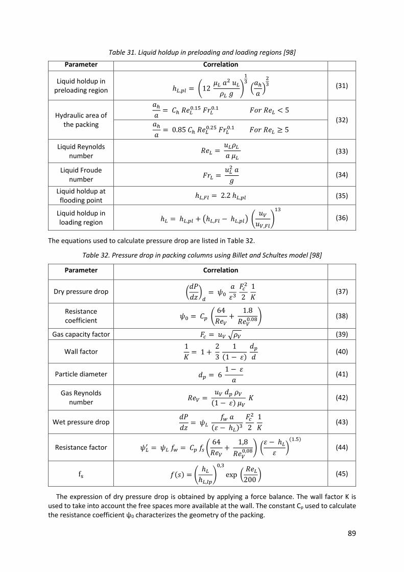
89
Table 31. Liquid holdup in preloading and loading regions [98]
Parameter Correlation
Liquid holdup in preloading region ℎ𝐿,𝑝𝑙 = (12
𝜇𝐿 𝑎2 𝑢𝐿
𝜌𝐿 𝑔)
13
(𝑎ℎ
𝑎)
23
(31)
Hydraulic area of the packing
𝑎ℎ
𝑎= 𝐶ℎ 𝑅𝑒𝐿
0.15 𝐹𝑟𝐿0.1 𝐹𝑜𝑟 𝑅𝑒𝐿 < 5
(32) 𝑎ℎ
𝑎= 0.85 𝐶ℎ 𝑅𝑒𝐿
0.25 𝐹𝑟𝐿0.1 𝐹𝑜𝑟 𝑅𝑒𝐿 ≥ 5
Liquid Reynolds number
𝑅𝑒𝐿 = 𝑢𝐿𝜌𝐿
𝑎 𝜇𝐿 (33)
Liquid Froude number
𝐹𝑟𝐿 = 𝑢𝐿
2 𝑎
𝑔 (34)
Liquid holdup at flooding point
ℎ𝐿,𝐹𝑙 = 2.2 ℎ𝐿,𝑝𝑙 (35)
Liquid holdup in loading region ℎ𝐿 = ℎ𝐿,𝑝𝑙 + (ℎ𝐿,𝐹𝑙 − ℎ𝐿,𝑝𝑙) (
𝑢𝑉
𝑢𝑉,𝐹𝑙)
13
(36)
The equations used to calculate pressure drop are listed in Table 32.
Table 32. Pressure drop in packing columns using Billet and Schultes model [98]
Parameter Correlation
Dry pressure drop (𝑑𝑃
𝑑𝑧)
𝑑= 𝜓0
𝑎
휀3 𝐹𝑐
2
2 1
𝐾 (37)
Resistance coefficient
𝜓0 = 𝐶𝑝 (64
𝑅𝑒𝑉+
1.8
𝑅𝑒𝑉0.08) (38)
Gas capacity factor 𝐹𝑐 = 𝑢𝑉 √𝜌𝑉 (39)
Wall factor 1
𝐾= 1 +
2
3
1
(1 − 휀) 𝑑𝑝
𝑑 (40)
Particle diameter 𝑑𝑝 = 6 1 − 휀
𝑎 (41)
Gas Reynolds number
𝑅𝑒𝑉 = 𝑢𝑉 𝑑𝑝 𝜌𝑉
(1 − 휀) 𝜇𝑉 𝐾 (42)
Wet pressure drop 𝑑𝑃
𝑑𝑧= 𝜓𝐿
𝑓𝑤 𝑎
(휀 − ℎ𝐿)3 𝐹𝑐
2
2 1
𝐾 (43)
Resistance factor 𝜓𝐿′ = 𝜓𝐿 𝑓𝑤 = 𝐶𝑝 𝑓𝑠 (
64
𝑅𝑒𝑉+
1,8
𝑅𝑒𝑉0,08) (
휀 − ℎ𝐿
휀)
(1.5)
(44)
fs 𝑓(𝑠) = (ℎ𝐿
ℎ𝐿,𝑙𝑝)
0,3
exp ( 𝑅𝑒𝐿
200 ) (45)
The expression of dry pressure drop is obtained by applying a force balance. The wall factor K is used to take into account the free spaces more available at the wall. The constant Cp used to calculate the resistance coefficient ψ0 characterizes the geometry of the packing.
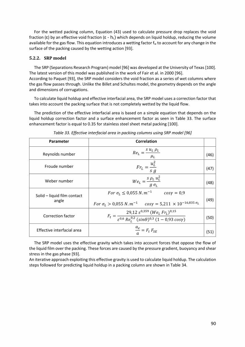
90
For the wetted packing column, Equation (43) used to calculate pressure drop replaces the void fraction (ε) by an effective void fraction (ε - hL) which depends on liquid holdup, reducing the volume available for the gas flow. This equation introduces a wetting factor fw to account for any change in the surface of the packing caused by the wetting action [93].
5.2.2. SRP model
The SRP (Separations Research Program) model [96] was developed at the University of Texas [100]. The latest version of this model was published in the work of Fair et al. in 2000 [96]. According to Paquet [93], the SRP model considers the void fraction as a series of wet columns where the gas flow passes through. Unlike the Billet and Schultes model, the geometry depends on the angle and dimensions of corrugations.
To calculate liquid holdup and effective interfacial area, the SRP model uses a correction factor that takes into account the packing surface that is not completely wetted by the liquid flow.
The prediction of the effective interfacial area is based on a simple equation that depends on the liquid holdup correction factor and a surface enhancement factor as seen in Table 33. The surface enhancement factor is equal to 0.35 for stainless steel sheet metal packing [100].
Table 33. Effective interfacial area in packing columns using SRP model [96]
Parameter Correlation
Reynolds number 𝑅𝑒𝐿 =𝑠 𝑢𝐿 𝜌𝐿
𝜇𝐿 (46)
Froude number 𝐹𝑟𝐿 =𝑢𝐿
2
𝑠 𝑔 (47)
Weber number 𝑊𝑒𝐿 =𝑠 𝜌𝐿 𝑢𝐿
2
𝑔 𝜎𝐿 (48)
Solid – liquid film contact angle
𝐹𝑜𝑟 𝜎𝐿 ≤ 0,055 𝑁. 𝑚−1 𝑐𝑜𝑠𝛾 = 0,9
𝐹𝑜𝑟 𝜎𝐿 > 0,055 𝑁. 𝑚−1 𝑐𝑜𝑠𝛾 = 5,211 × 10−16,835 𝜎𝐿 (49)
Correction factor 𝐹𝑡 =29,12 𝑠0,359 (𝑊𝑒𝐿 𝐹𝑟𝐿)0,15
휀0,6 𝑅𝑒𝐿0,2 (𝑠𝑖𝑛𝛳)0,3 (1 − 0,93 𝑐𝑜𝑠𝛾)
(50)
Effective interfacial area 𝑎𝑒
𝑎= 𝐹𝑡 𝐹𝑆𝐸 (51)
The SRP model uses the effective gravity which takes into account forces that oppose the flow of the liquid film over the packing. These forces are caused by the pressure gradient, buoyancy and shear stress in the gas phase [93]. An iterative approach exploiting this effective gravity is used to calculate liquid holdup. The calculation steps followed for predicting liquid holdup in a packing column are shown in Table 34.
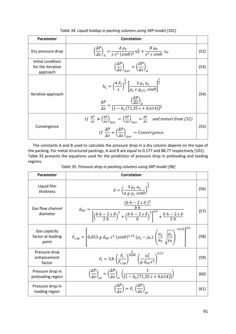
91
Table 34. Liquid holdup in packing columns using SRP model [101]
Parameter Correlation
Dry pressure drop (𝛥𝑃
𝛥𝑧)
𝑑=
𝐴 𝜌𝑉
𝑠 휀2 (𝑠𝑖𝑛𝛳)2𝑢𝑉
2 +𝐵 𝜇𝑉
𝑠2 휀 𝑠𝑖𝑛𝛳 𝑢𝑉 (52)
Initial condition for the iterative
approach (
𝛥𝑃
𝛥𝑧)
𝑖𝑡𝑒𝑟= (
𝛥𝑃
𝛥𝑧)
𝑑 (53)
Iterative approach
ℎ𝐿 = (4 𝐹𝑡
𝑠)
23
[3 𝜇𝐿 𝑢𝐿
𝜌𝐿 휀 𝑔𝑒𝑓𝑓 𝑠𝑖𝑛𝛳]
13
𝛥𝑃
𝛥𝑧=
(𝛥𝑃𝛥𝑧)
𝑑
[1 − ℎ𝐿(71,35 𝑠 + 0,614)]5
(54)
Convergence
𝐼𝑓 𝛥𝑃
𝛥𝑧 ≠ (
𝛥𝑃
𝛥𝑧)
𝑖𝑡𝑒𝑟→ (
𝛥𝑃
𝛥𝑧)
𝑖𝑡𝑒𝑟=
𝛥𝑃
𝛥𝑧 and restart from (52)
𝐼𝑓 𝛥𝑃
𝛥𝑧≈ (
𝛥𝑃
𝛥𝑧)
𝑖𝑡𝑒𝑟→ 𝐶𝑜𝑛𝑣𝑒𝑟𝑔𝑒𝑛𝑐𝑒
(55)
The constants A and B used to calculate the pressure drop in a dry column depend on the type of the packing. For metal structured packings, A and B are equal to 0.177 and 88.77 respectively [101]. Table 35 presents the equations used for the prediction of pressure drop in preloading and loading regions.
Table 35. Pressure drop in packing columns using SRP model [96]
Parameter Correlation
Liquid film thickness 𝛿 = (
3 𝜇𝐿 𝑢𝐿
𝑎 𝑔 𝜌𝐿 𝑠𝑖𝑛𝛳)
13
(56)
Gas flow channel diameter
𝑑ℎ𝑉 =
(𝑏 ℎ − 2 𝑠 𝛿 )2
𝑏 ℎ
[(𝑏 ℎ − 2 𝑠 𝛿
2 ℎ)
2
+ (𝑏 ℎ − 2 𝑠 𝛿
𝑏)
2
]
0,5
+𝑏 ℎ − 2 𝑠 𝛿
2 ℎ
(57)
Gas capacity factor at loading
point 𝐹𝑐,𝑙𝑝 = [0,053 𝑔 𝑑ℎ𝑉 휀2 (𝑠𝑖𝑛𝛳)1,15 (𝜌𝐿 − 𝜌𝑉) (
𝑢𝐿
𝑢𝑉 √
𝜌𝐿
𝜌𝑉)
−0,25
]
0,5
(58)
Pressure drop enhancement
factor 𝐹𝑙 = 3,8 (
𝐹𝑐
𝐹𝑐,𝑙𝑝)
2𝑠𝑖𝑛𝛳
(𝑢𝐿
2
𝑔 𝑑ℎ𝑉휀2)
0,13
(59)
Pressure drop in preloading region
(𝛥𝑃
𝛥𝑧)
𝑝𝑙= (
𝛥𝑃
𝛥𝑧)
𝑑 (
1
[1 − ℎ𝐿(71,35 𝑠 + 0,614)]) (60)
Pressure drop in loading region
(𝛥𝑃
𝛥𝑧) = 𝐹𝑙 (
𝛥𝑃
𝛥𝑧)
𝑝𝑙 (61)
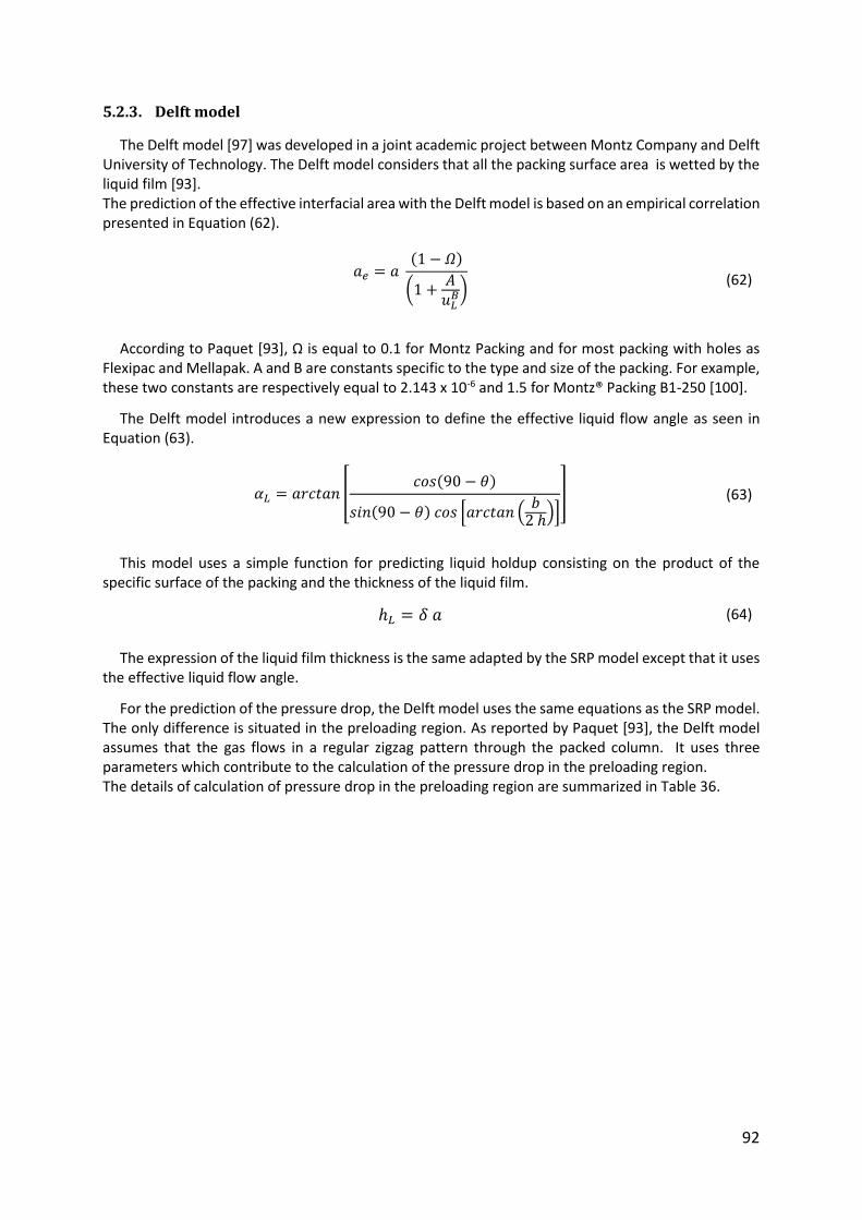
92
5.2.3. Delft model
The Delft model [97] was developed in a joint academic project between Montz Company and Delft University of Technology. The Delft model considers that all the packing surface area is wetted by the liquid film [93]. The prediction of the effective interfacial area with the Delft model is based on an empirical correlation presented in Equation (62).
𝑎𝑒 = 𝑎 (1 − 𝛺)
(1 +𝐴
𝑢𝐿𝐵)
(62)
According to Paquet [93], Ω is equal to 0.1 for Montz Packing and for most packing with holes as Flexipac and Mellapak. A and B are constants specific to the type and size of the packing. For example, these two constants are respectively equal to 2.143 x 10⁻⁶ and 1.5 for Montz® Packing B1-250 [100].
The Delft model introduces a new expression to define the effective liquid flow angle as seen in Equation (63).
𝛼𝐿 = 𝑎𝑟𝑐𝑡𝑎𝑛 [𝑐𝑜𝑠(90 − 𝜃)
𝑠𝑖𝑛(90 − 𝜃) 𝑐𝑜𝑠 [𝑎𝑟𝑐𝑡𝑎𝑛 (𝑏
2 ℎ)]
] (63)
This model uses a simple function for predicting liquid holdup consisting on the product of the specific surface of the packing and the thickness of the liquid film.
ℎ𝐿 = 𝛿 𝑎 (64)
The expression of the liquid film thickness is the same adapted by the SRP model except that it uses the effective liquid flow angle.
For the prediction of the pressure drop, the Delft model uses the same equations as the SRP model. The only difference is situated in the preloading region. As reported by Paquet [93], the Delft model assumes that the gas flows in a regular zigzag pattern through the packed column. It uses three parameters which contribute to the calculation of the pressure drop in the preloading region. The details of calculation of pressure drop in the preloading region are summarized in Table 36.
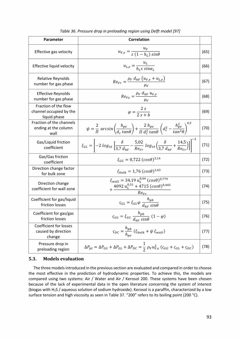
93
Table 36. Pressure drop in preloading region using Delft model [97]
Parameter Correlation
Effective gas velocity 𝑢𝑉,𝑒 =𝑢𝑉
휀 (1 − ℎ𝐿) 𝑠𝑖𝑛𝜃 (65)
Effective liquid velocity 𝑢𝐿,𝑒 =𝑢𝐿
ℎ𝐿휀 𝑠𝑖𝑛𝛼𝐿 (66)
Relative Reynolds number for gas phase 𝑅𝑒𝑉𝑟 =
𝜌𝑉 𝑑ℎ𝑉 (𝑢𝑉,𝑒 + 𝑢𝐿,𝑒)
𝜇𝑉 (67)
Effective Reynolds number for gas phase
𝑅𝑒𝑉𝑒 =𝜌𝑉 𝑑ℎ𝑉 𝑢𝑉,𝑒
𝜇𝑉 (68)
Fraction of the flow channel occupied by the
liquid phase 𝜑 =
2 𝑠
2 𝑠 + 𝑏 (69)
Fraction of the channels ending at the column
wall 𝜓 =
2
𝛱 𝑎𝑟𝑐𝑠𝑖𝑛 (
ℎ𝑝𝑒
𝑑𝑐 𝑡𝑎𝑛𝜃) +
2 ℎ𝑝𝑒
𝛱 𝑑𝑐2 𝑡𝑎𝑛𝜃
(𝑑𝑐2 −
ℎ𝑝𝑒2
𝑡𝑎𝑛2𝜃)
0,5
(70)
Gas/Liquid friction coefficient 𝜉𝐺𝐿 = [−2 𝑙𝑜𝑔10 [
𝛿
3,7 𝑑ℎ𝑉−
5,02
𝑅𝑒𝑉𝑟 𝑙𝑜𝑔10 (
𝛿
3,7 𝑑ℎ𝑉+
14,5
𝑅𝑒𝑉𝑟)]]
−2
(71)
Gas/Gas friction coefficient
𝜉𝐺𝐺 = 0,722 (𝑐𝑜𝑠𝜃)3,14 (72)
Direction change factor for bulk zone
𝜉𝑏𝑢𝑙𝑘 = 1,76 (𝑐𝑜𝑠𝜃)1,63 (73)
Direction change coefficient for wall zone
𝜉𝑤𝑎𝑙𝑙 = 34,19 𝑢𝐿0,44 (𝑐𝑜𝑠𝜃)0,779
+4092 𝑢𝐿
0,31 + 4715 (𝑐𝑜𝑠𝜃)0,445
𝑅𝑒𝑉𝑒
(74)
Coefficient for gas/liquid friction losses
𝜍𝐺𝐿 = 𝜉𝐺𝐿𝜑 ℎ𝑝𝑏
𝑑ℎ𝑉 𝑠𝑖𝑛𝜃 (75)
Coefficient for gas/gas friction losses
𝜍𝐺𝐺 = 𝜉𝐺𝐺 ℎ𝑝𝑏
𝑑ℎ𝑉 𝑠𝑖𝑛𝜃 (1 − 𝜑) (76)
Coefficient for losses caused by direction
change 𝜍𝐷𝐶 =
ℎ𝑝𝑏
ℎ𝑝𝑒 (𝜉𝑏𝑢𝑙𝑘 + 𝜓 𝜉𝑤𝑎𝑙𝑙) (77)
Pressure drop in preloading region ∆𝑃𝑝𝑙 = ∆𝑃𝐺𝐺 + ∆𝑃𝐺𝐿 + ∆𝑃𝐷𝐶 =
1
2 𝜌𝑉𝑢𝑉,𝑒
2 (𝜍𝐺𝐺 + 𝜍𝐺𝐿 + 𝜍𝐷𝐶) (78)
5.3. Models evaluation
The three models introduced in the previous section are evaluated and compared in order to choose the most effective in the prediction of hydrodynamic properties. To achieve this, the models are compared using two systems: Air / Water and Air / Kerosol 200. These systems have been chosen because of the lack of experimental data in the open literature concerning the system of interest (biogas with H2S / aqueous solution of sodium hydroxide). Kerosol is a paraffin, characterized by a low surface tension and high viscosity as seen in Table 37. “200” refers to its boiling point (200 °C).
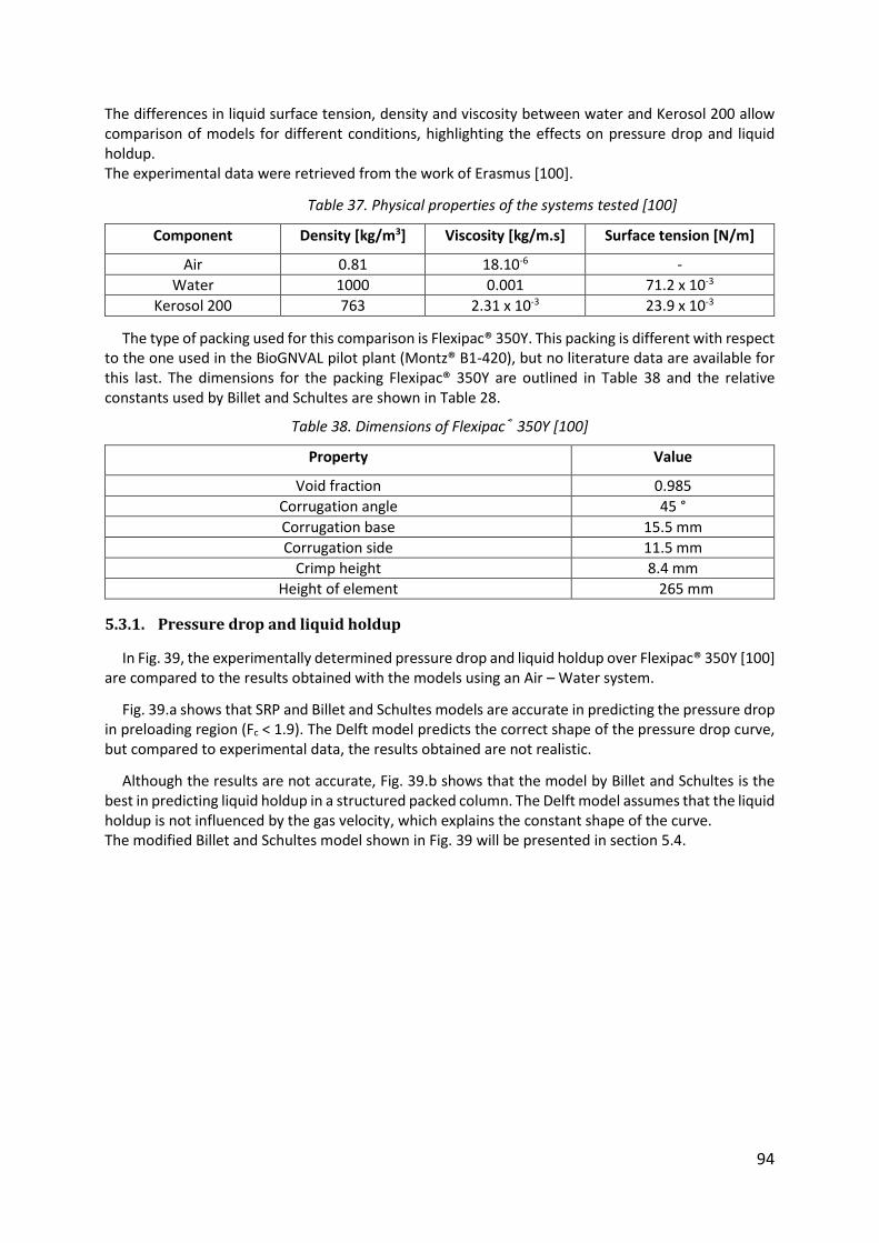
94
The differences in liquid surface tension, density and viscosity between water and Kerosol 200 allow comparison of models for different conditions, highlighting the effects on pressure drop and liquid holdup. The experimental data were retrieved from the work of Erasmus [100].
Table 37. Physical properties of the systems tested [100]
Component Density [kg/m3] Viscosity [kg/m.s] Surface tension [N/m]
Air 0.81 18.10-6 -
Water 1000 0.001 71.2 x 10⁻³
Kerosol 200 763 2.31 x 10⁻³ 23.9 x 10⁻³
The type of packing used for this comparison is Flexipac® 350Y. This packing is different with respect to the one used in the BioGNVAL pilot plant (Montz® B1-420), but no literature data are available for this last. The dimensions for the packing Flexipac® 350Y are outlined in Table 38 and the relative constants used by Billet and Schultes are shown in Table 28.
Table 38. Dimensions of Flexipac® 350Y [100]
Property Value
Void fraction 0.985
Corrugation angle 45 °
Corrugation base 15.5 mm
Corrugation side 11.5 mm
Crimp height 8.4 mm
Height of element 265 mm
5.3.1. Pressure drop and liquid holdup
In Fig. 39, the experimentally determined pressure drop and liquid holdup over Flexipac® 350Y [100] are compared to the results obtained with the models using an Air – Water system.
Fig. 39.a shows that SRP and Billet and Schultes models are accurate in predicting the pressure drop in preloading region (Fc < 1.9). The Delft model predicts the correct shape of the pressure drop curve, but compared to experimental data, the results obtained are not realistic.
Although the results are not accurate, Fig. 39.b shows that the model by Billet and Schultes is the best in predicting liquid holdup in a structured packed column. The Delft model assumes that the liquid holdup is not influenced by the gas velocity, which explains the constant shape of the curve. The modified Billet and Schultes model shown in Fig. 39 will be presented in section 5.4.

95
Fig. 39.a. Pressure drop evaluation for liquid load uL = 20.5 m/h
Models: (__Δ__) Billet & Schultes ; (- -□- -) SRP ; (- .○- .) Delft ; (…+…) Billet & Schultes modified “Section 5” ; Experimental
values: (♦) [100]
Fig. 39.b. Liquid holdup evaluation for liquid load uL = 20.5 m/h
Models: (__Δ__) Billet & Schultes ; (- -□- -) SRP ; (- .○- .) Delft ; (…+…) Billet & Schultes modified “Section 5” ; Experimental
values: (♦) [100]
0
200
400
600
800
1000
1200
0 0.5 1 1.5 2 2.5 3 3.5 4 4.5
Pre
ssu
re d
rop
[P
a/m
]
Vapor capacity factor [(m/s).(kg/m3)0.5]
0
0.02
0.04
0.06
0.08
0.1
0.12
0.14
0.16
0 0.5 1 1.5 2 2.5 3 3.5 4 4.5 5
Liq
uid
ho
ldu
p [
m3 /
m3]
Vapor capacity factor [(m/s).(kg/m3)0.5]

96
The average absolute deviations between predictive models (Billet & Schultes, SRP and Delft) and experimental results for pressure drop and liquid holdup are shown in Table 39.
Table 39. Deviation between predictive models and experimental data
Model Average Absolute Deviation AAD [%]
Pressure drop Liquid holdup
Billet and Schultes 36 35
SRP 41 44
Delft 481 22
Modified Billet and Schultes model
6 10
5.3.2. Effective interfacial area
In a packed column, the gas and the liquid phases are brought into contact and exchange mass and energy across their common interfacial area. The effective interfacial area accounts for the dead area that does not actively take part in the mass transfer process.
Fig. 40 shows the results of the effective interfacial area obtained with the three models, and compared to experimental data.
Fig. 40.a. Prediction of effective interfacial area by Billet and Schultes model for the system Air / Kerosol 200
Models: (__Δ__) Billet & Schultes ; (♦) Experimental values [100]
0
50
100
150
200
250
0 5 10 15 20 25 30
Effe
ctiv
e in
terf
acia
l are
a [m
2 /m
3]
Liquid load [m/h]
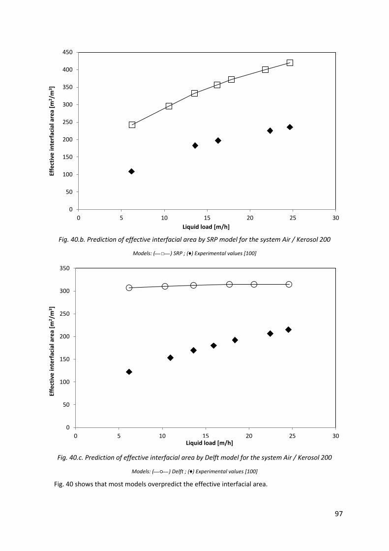
97
Fig. 40.b. Prediction of effective interfacial area by SRP model for the system Air / Kerosol 200
Models: (__□__) SRP ; (♦) Experimental values [100]
Fig. 40.c. Prediction of effective interfacial area by Delft model for the system Air / Kerosol 200
Models: (__○__) Delft ; (♦) Experimental values [100]
Fig. 40 shows that most models overpredict the effective interfacial area.
0
50
100
150
200
250
300
350
400
450
0 5 10 15 20 25 30
Effe
ctiv
e in
terf
acia
l are
a [m
2 /m
3]
Liquid load [m/h]
0
50
100
150
200
250
300
350
0 5 10 15 20 25 30
Effe
ctiv
e in
terf
acia
l are
a [m
2 /m
3 ]
Liquid load [m/h]
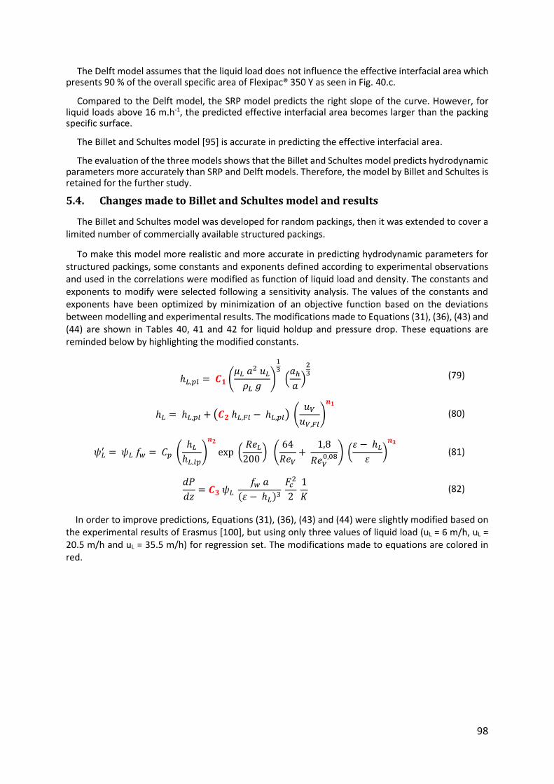
98
The Delft model assumes that the liquid load does not influence the effective interfacial area which presents 90 % of the overall specific area of Flexipac® 350 Y as seen in Fig. 40.c.
Compared to the Delft model, the SRP model predicts the right slope of the curve. However, for liquid loads above 16 m.h-1, the predicted effective interfacial area becomes larger than the packing specific surface.
The Billet and Schultes model [95] is accurate in predicting the effective interfacial area.
The evaluation of the three models shows that the Billet and Schultes model predicts hydrodynamic parameters more accurately than SRP and Delft models. Therefore, the model by Billet and Schultes is retained for the further study.
5.4. Changes made to Billet and Schultes model and results
The Billet and Schultes model was developed for random packings, then it was extended to cover a limited number of commercially available structured packings.
To make this model more realistic and more accurate in predicting hydrodynamic parameters for structured packings, some constants and exponents defined according to experimental observations and used in the correlations were modified as function of liquid load and density. The constants and exponents to modify were selected following a sensitivity analysis. The values of the constants and exponents have been optimized by minimization of an objective function based on the deviations between modelling and experimental results. The modifications made to Equations (31), (36), (43) and (44) are shown in Tables 40, 41 and 42 for liquid holdup and pressure drop. These equations are reminded below by highlighting the modified constants.
ℎ𝐿,𝑝𝑙 = 𝑪𝟏 (𝜇𝐿 𝑎2 𝑢𝐿
𝜌𝐿 𝑔)
13
(𝑎ℎ
𝑎)
23 (79)
ℎ𝐿 = ℎ𝐿,𝑝𝑙 + (𝑪𝟐 ℎ𝐿,𝐹𝑙 − ℎ𝐿,𝑝𝑙) (𝑢𝑉
𝑢𝑉,𝐹𝑙)
𝒏𝟏
(80)
𝜓𝐿′ = 𝜓𝐿 𝑓𝑤 = 𝐶𝑝 (
ℎ𝐿
ℎ𝐿,𝑙𝑝)
𝒏𝟐
exp ( 𝑅𝑒𝐿
200 ) (
64
𝑅𝑒𝑉+
1,8
𝑅𝑒𝑉0,08) (
휀 − ℎ𝐿
휀)
𝒏𝟑
(81)
𝑑𝑃
𝑑𝑧= 𝑪𝟑 𝜓𝐿
𝑓𝑤 𝑎
(휀 − ℎ𝐿)3 𝐹𝑐
2
2 1
𝐾 (82)
In order to improve predictions, Equations (31), (36), (43) and (44) were slightly modified based on the experimental results of Erasmus [100], but using only three values of liquid load (uL = 6 m/h, uL = 20.5 m/h and uL = 35.5 m/h) for regression set. The modifications made to equations are colored in red.

99
Table 40. Changes made to calculate liquid holdup
Equations to modify
New equations
(79)
For liquid density > 900 kg/m3
ℎ𝐿,𝑝𝑙 = [𝟔𝟐𝟖. 𝟒 ∗ (𝒖𝑳 ∗ 𝟑𝟔𝟎𝟎)−𝟎.𝟗𝟐𝟗]𝟏𝟑 (
𝜇𝐿 𝑎2 𝑢𝐿
𝜌𝐿 𝑔)
13
(𝑎ℎ
𝑎)
23
For liquid density ≤ 900 kg/m3
ℎ𝐿,𝑝𝑙 = 𝑬𝒙𝒑(−𝟎. 𝟎𝟎𝟓𝟕 ∗ 𝒖𝑳 ∗ 𝟑𝟔𝟎𝟎 + 𝟏. 𝟐𝟎𝟕𝟒) (𝜇𝐿 𝑎2 𝑢𝐿
𝜌𝐿 𝑔)
13
(𝑎ℎ
𝑎)
23
(80)
For liquid density > 900 kg/m3
ℎ𝐿 = ℎ𝐿,𝑝𝑙 + (𝟏, 𝟑 ℎ𝐿,𝐹𝑙 − ℎ𝐿,𝑝𝑙) (𝑢𝑉
𝑢𝑉,𝐹𝑙)
𝟏𝟎
For liquid density ≤ 900 kg/m3
ℎ𝐿 = ℎ𝐿,𝑝𝑙 + (𝑬𝒙𝒑 [−𝟎. 𝟎𝟎𝟎𝟔 ∗ (𝒖𝑳 ∗ 𝟑𝟔𝟎𝟎)𝟐 − 𝟎. 𝟎𝟑𝟏 ∗ 𝒖𝑳 ∗ 𝟑𝟔𝟎𝟎 + 𝟎. 𝟑𝟕𝟑𝟔]
∗ ℎ𝐿,𝐹𝑙 − ℎ𝐿,𝑝𝑙) (𝑢𝑉
𝑢𝑉,𝐹𝑙)
[−𝟎.𝟎𝟐𝟏𝟓∗ (𝒖𝑳∗𝟑𝟔𝟎𝟎)𝟐 + 𝟎.𝟖𝟗𝟐𝟕∗ 𝒖𝑳∗𝟑𝟔𝟎𝟎 + 𝟓.𝟑𝟑𝟓𝟖]
Table 41. Changes made to calculate Pressure drop for liquid density less than 900 kg.m-3
Equations to modify
New equations
(81)
Preloading region
𝜓𝐿′ = 𝜓𝐿 𝑓𝑤 = 𝐶𝑝 (
ℎ𝐿
ℎ𝐿,𝑙𝑝)
𝟎.𝟑
exp ( 𝑅𝑒𝐿
200 ) (
64
𝑅𝑒𝑉+
1,8
𝑅𝑒𝑉0,08) (
𝜀− ℎ𝐿
𝜀)
𝟏.𝟓
Loading & Flooding regions
𝜓𝐿′ = 𝜓𝐿 𝑓𝑤 = 𝐶𝑝 (
ℎ𝐿
ℎ𝐿,𝑙𝑝)
𝟎.𝟔
exp ( 𝑅𝑒𝐿
200 ) (
64
𝑅𝑒𝑉+
1,8
𝑅𝑒𝑉0,08) (
𝜀− ℎ𝐿
𝜀)
𝟎.𝟓
(82)
Preloading region
𝑑𝑃
𝑑𝑧= 𝑬𝒙𝒑 (𝟎. 𝟎𝟏𝟒𝟗 ∗ 𝒖𝑳 ∗ 𝟑𝟔𝟎𝟎 + 𝟎. 𝟎𝟖𝟐𝟗) 𝜓𝐿
𝑓𝑤 𝑎
(𝜀− ℎ𝐿)3 𝐹𝑐
2
2
1
𝐾
Loading & Flooding regions
𝑑𝑃
𝑑𝑧= 𝟎. 𝟎𝟎𝟐 ∗ (𝒖𝑳 ∗ 𝟑𝟔𝟎𝟎)𝟐 − 𝟎. 𝟎𝟓𝟑𝟒 ∗ 𝒖𝑳 + 𝟏. 𝟕𝟔 𝜓𝐿
𝑓𝑤 𝑎
(𝜀− ℎ𝐿)3 𝐹𝑐
2
2
1
𝐾

100
Table 42. Changes made to calculate Pressure drop for liquid density higher than 900 kg.m-3
The refined model is then compared to an extended range of experimental data retrieved also from the work of Erasmus [100] in order to validate the new model.
Comparisons to validate the modified model were made at various liquid loads and using two different systems: Air – Water and Air – Kerosol 200. Results of liquid holdup and pressure drop of the two systems over Flexipac® 350Y are presented in Fig. 41 and 42.
The same conditions used to evaluate the three models (Type of packing: Flexipac® 350Y, system: Air – Water, Liquid load: 20.5 m/h) are used again in order to evaluate the new model and compare it to the other ones and to the experimental data. In Fig. 39, the experimentally determined pressure drop and liquid holdup [100] are compared to the results obtained with all the models including the new one.
Table 39 presents the deviations between predictive models (Billet & Schultes, SRP and Delft), the modified Billet and Schultes model and experimental results for pressure drop and liquid holdup.
Equation to modify
New equations
(81)
Preloading region
𝜓𝐿′ = 𝜓𝐿 𝑓𝑤 = 𝐶𝑝 (
ℎ𝐿
ℎ𝐿,𝑙𝑝)
𝟎.𝟑
exp ( 𝑅𝑒𝐿
200 ) (
64
𝑅𝑒𝑉+
1,8
𝑅𝑒𝑉0,08) (
𝜀− ℎ𝐿
𝜀)
𝟏.𝟓
Loading region (For hL > hL,lp)
𝜓𝐿′ = 𝜓𝐿 𝑓𝑤 = 𝐶𝑝 (
ℎ𝐿
ℎ𝐿,𝑙𝑝)
𝟓
exp ( 𝑅𝑒𝐿
200 ) (
64
𝑅𝑒𝑉+
1,8
𝑅𝑒𝑉0,08) (
𝜀− ℎ𝐿
𝜀)
𝟏𝟐
Loading region (For hL ≤ hL,lp)
𝜓𝐿′ = 𝜓𝐿 𝑓𝑤 = 𝐶𝑝 (
ℎ𝐿
ℎ𝐿,𝑙𝑝)
𝟎.𝟑
exp ( 𝑅𝑒𝐿
200 ) (
64
𝑅𝑒𝑉+
1,8
𝑅𝑒𝑉0,08) (
𝜀− ℎ𝐿
𝜀)
𝟑
Flooding region
𝜓𝐿′ = 𝜓𝐿 𝑓𝑤 = 𝐶𝑝 (
ℎ𝐿
ℎ𝐿,𝑙𝑝)
𝟎.𝟔
exp ( 𝑅𝑒𝐿
200 ) (
64
𝑅𝑒𝑉+
1,8
𝑅𝑒𝑉0,08) (
𝜀− ℎ𝐿
𝜀)
𝟏.𝟓
(82)
Preloading region
𝑑𝑃
𝑑𝑧= 𝟏. 𝟐 𝜓𝐿
𝑓𝑤 𝑎
(𝜀− ℎ𝐿)3 𝐹𝑐
2
2
1
𝐾
Loading region
𝑑𝑃
𝑑𝑧= 𝟏. 𝟓 𝜓𝐿
𝑓𝑤 𝑎
(𝜀− ℎ𝐿)3 𝐹𝑐
2
2
1
𝐾
Flooding region
𝑑𝑃
𝑑𝑧= 𝟏. 𝟒 𝜓𝐿
𝑓𝑤 𝑎
(𝜀− ℎ𝐿)3 𝐹𝑐
2
2
1
𝐾
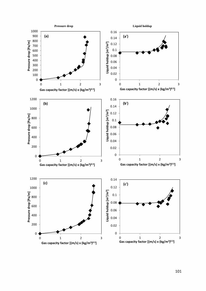
101
Pressure drop Liquid holdup
0
100
200
300
400
500
600
700
800
900
1000
0 1 2 3
Pre
ssu
re d
rop
[P
a/m
]
Gas capacity factor [(m/s) x (kg/m3)0.5]
(a)
0
0.02
0.04
0.06
0.08
0.1
0.12
0.14
0.16
0 1 2 3
Liq
uid
ho
ldu
p [
m3/m
3 ]
Gas capacity factor [(m/s) x (kg/m3)0.5]
(a')
0
200
400
600
800
1000
1200
0 1 2 3
Pre
ssu
re d
rop
[P
a/m
]
Gas capacity factor [(m/s) x (kg/m3)0.5]
(b)
0
0.02
0.04
0.06
0.08
0.1
0.12
0.14
0.16
0 1 2 3
Liq
uid
ho
ldu
p [
m3 /
m3 ]
Gas capacity factor [(m/s) x (kg/m3)0.5]
(b')
0
200
400
600
800
1000
1200
0 1 2 3
Pre
ssu
re d
rop
[P
a/m
]
Gas capacity factor [(m/s) x (kg/m3)0.5]
(c)
0
0.02
0.04
0.06
0.08
0.1
0.12
0.14
0 1 2 3
Liq
uid
ho
ldu
p [
m3 /
m3 ]
Gas capacity factor [(m/s) x (kg/m3)0.5]
(c')

102
Fig. 41. Liquid holdup and pressure drop with an Air – Water system using Flexipac® 350Y packing
Models: (―) Billet & Schultes modified ; (♦) Experimental values [100] Liquid loads: (a), (a’) uL = 35.6 m/h ; (b), (b’) uL = 28.8 m/h ; (c), (c’) uL = 20.5 m/h ; (d), (d’) uL = 12.9 m/h ; (e), (e’) uL = 6
m/h
0
200
400
600
800
1000
1200
1400
0 1 2 3 4
Pre
ssu
re d
rop
[P
a/m
]
Gas capacity factor [(m/s) x (kg/m3)0.5]
(d)
0
0.02
0.04
0.06
0.08
0.1
0.12
0 1 2 3 4
Liq
uid
ho
ldu
p [
m3 /
m3 ]
Gas capacity factor [(m/s) x (kg/m3)0.5]
(d')
0
200
400
600
800
1000
1200
1400
0 1 2 3 4
Pre
ssu
re d
rop
[P
a/m
]
Gas capacity factor [(m/s) x (kg/m3)0.5]
(e)
0
0.01
0.02
0.03
0.04
0.05
0.06
0.07
0.08
0.09
0 1 2 3 4
Liq
uid
ho
ldu
p [
m3/m
3 ]
Gas capacity factor [(m/s) x (kg/m3)0.5]
(e')
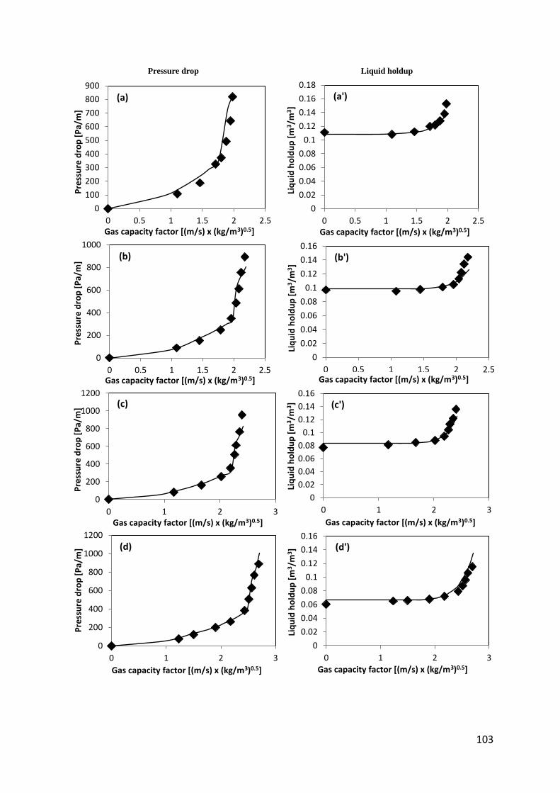
103
Pressure drop Liquid holdup
0
100
200
300
400
500
600
700
800
900
0 0.5 1 1.5 2 2.5
Pre
ssu
re d
rop
[P
a/m
]
Gas capacity factor [(m/s) x (kg/m3)0.5]
(a)
0
0.02
0.04
0.06
0.08
0.1
0.12
0.14
0.16
0.18
0 0.5 1 1.5 2 2.5
Liq
uid
ho
ldu
p [
m3/m
3]
Gas capacity factor [(m/s) x (kg/m3)0.5]
(a')
0
200
400
600
800
1000
0 0.5 1 1.5 2 2.5
Pre
ssu
re d
rop
[P
a/m
]
Gas capacity factor [(m/s) x (kg/m3)0.5]
(b)
0
0.02
0.04
0.06
0.08
0.1
0.12
0.14
0.16
0 0.5 1 1.5 2 2.5
Liq
uid
ho
ldu
p [
m3 /
m3 ]
Gas capacity factor [(m/s) x (kg/m3)0.5]
(b')
0
200
400
600
800
1000
1200
0 1 2 3
Pre
ssu
re d
rop
[P
a/m
]
Gas capacity factor [(m/s) x (kg/m3)0.5]
(c)
0
0.02
0.04
0.06
0.08
0.1
0.12
0.14
0.16
0 1 2 3
Liq
uid
ho
ldu
p [
m3/m
3]
Gas capacity factor [(m/s) x (kg/m3)0.5]
(c')
0
200
400
600
800
1000
1200
0 1 2 3
Pre
ssu
re d
rop
[P
a/m
]
Gas capacity factor [(m/s) x (kg/m3)0.5]
(d)
0
0.02
0.04
0.06
0.08
0.1
0.12
0.14
0.16
0 1 2 3
Liq
uid
ho
ldu
p [
m3 /
m3]
Gas capacity factor [(m/s) x (kg/m3)0.5]
(d')
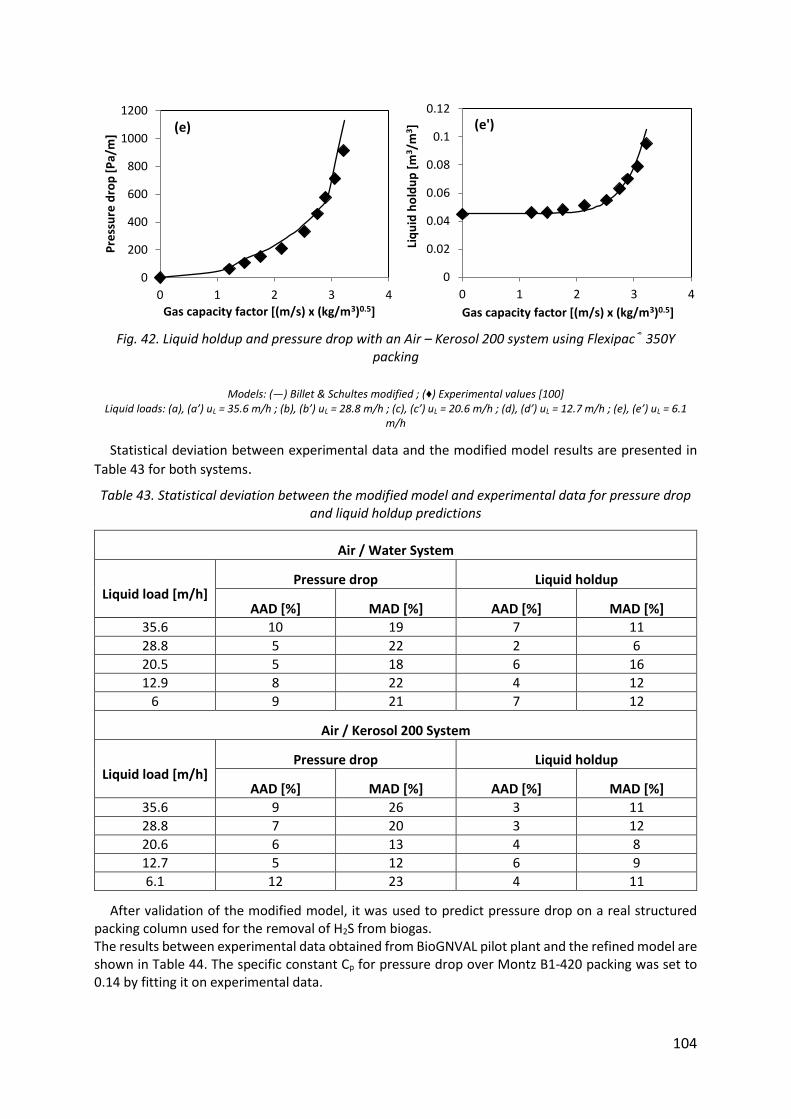
104
Fig. 42. Liquid holdup and pressure drop with an Air – Kerosol 200 system using Flexipac® 350Y packing
Models: (―) Billet & Schultes modified ; (♦) Experimental values [100] Liquid loads: (a), (a’) uL = 35.6 m/h ; (b), (b’) uL = 28.8 m/h ; (c), (c’) uL = 20.6 m/h ; (d), (d’) uL = 12.7 m/h ; (e), (e’) uL = 6.1
m/h
Statistical deviation between experimental data and the modified model results are presented in
Table 43 for both systems.
Table 43. Statistical deviation between the modified model and experimental data for pressure drop and liquid holdup predictions
Air / Water System
Liquid load [m/h] Pressure drop Liquid holdup
AAD [%] MAD [%] AAD [%] MAD [%] 35.6 10 19 7 11
28.8 5 22 2 6
20.5 5 18 6 16
12.9 8 22 4 12
6 9 21 7 12
Air / Kerosol 200 System
Liquid load [m/h] Pressure drop Liquid holdup
AAD [%] MAD [%] AAD [%] MAD [%]
35.6 9 26 3 11
28.8 7 20 3 12
20.6 6 13 4 8
12.7 5 12 6 9
6.1 12 23 4 11
After validation of the modified model, it was used to predict pressure drop on a real structured packing column used for the removal of H2S from biogas. The results between experimental data obtained from BioGNVAL pilot plant and the refined model are shown in Table 44. The specific constant Cp for pressure drop over Montz B1-420 packing was set to 0.14 by fitting it on experimental data.
0
200
400
600
800
1000
1200
0 1 2 3 4
Pre
ssu
re d
rop
[P
a/m
]
Gas capacity factor [(m/s) x (kg/m3)0.5]
(e)
0
0.02
0.04
0.06
0.08
0.1
0.12
0 1 2 3 4
Liq
uid
ho
ldu
p [
m3 /
m3 ]
Gas capacity factor [(m/s) x (kg/m3)0.5]
(e')
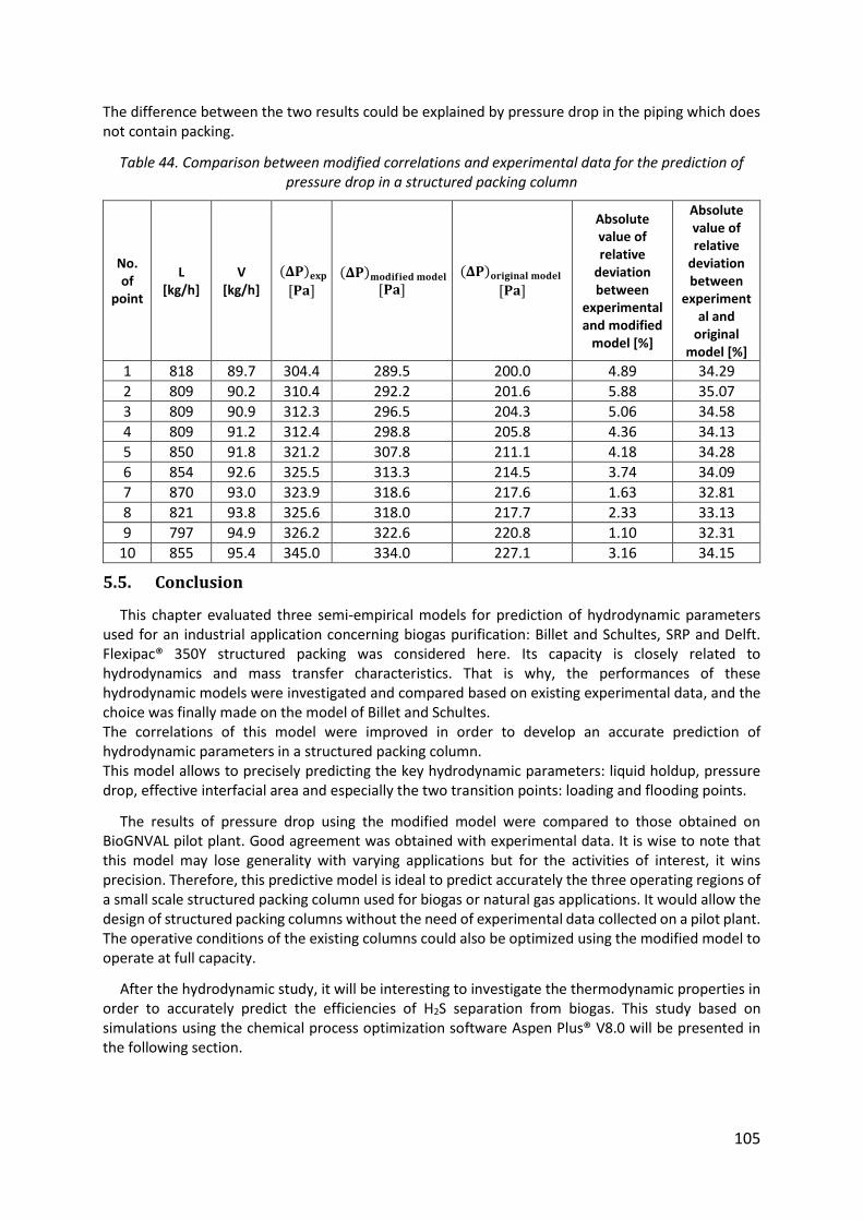
105
The difference between the two results could be explained by pressure drop in the piping which does not contain packing.
Table 44. Comparison between modified correlations and experimental data for the prediction of pressure drop in a structured packing column
No. of
point
L [kg/h]
V [kg/h]
(𝚫𝐏)𝐞𝐱𝐩 [𝐏𝐚]
(𝚫𝐏)𝐦𝐨𝐝𝐢𝐟𝐢𝐞𝐝 𝐦𝐨𝐝𝐞𝐥 [𝐏𝐚]
(𝚫𝐏)𝐨𝐫𝐢𝐠𝐢𝐧𝐚𝐥 𝐦𝐨𝐝𝐞𝐥 [𝐏𝐚]
Absolute value of relative
deviation between
experimental and modified
model [%]
Absolute value of relative
deviation between
experimental and
original model [%]
1 818 89.7 304.4 289.5 200.0 4.89 34.29
2 809 90.2 310.4 292.2 201.6 5.88 35.07
3 809 90.9 312.3 296.5 204.3 5.06 34.58
4 809 91.2 312.4 298.8 205.8 4.36 34.13
5 850 91.8 321.2 307.8 211.1 4.18 34.28
6 854 92.6 325.5 313.3 214.5 3.74 34.09
7 870 93.0 323.9 318.6 217.6 1.63 32.81
8 821 93.8 325.6 318.0 217.7 2.33 33.13
9 797 94.9 326.2 322.6 220.8 1.10 32.31
10 855 95.4 345.0 334.0 227.1 3.16 34.15
5.5. Conclusion
This chapter evaluated three semi-empirical models for prediction of hydrodynamic parameters used for an industrial application concerning biogas purification: Billet and Schultes, SRP and Delft. Flexipac® 350Y structured packing was considered here. Its capacity is closely related to hydrodynamics and mass transfer characteristics. That is why, the performances of these hydrodynamic models were investigated and compared based on existing experimental data, and the choice was finally made on the model of Billet and Schultes. The correlations of this model were improved in order to develop an accurate prediction of hydrodynamic parameters in a structured packing column. This model allows to precisely predicting the key hydrodynamic parameters: liquid holdup, pressure drop, effective interfacial area and especially the two transition points: loading and flooding points.
The results of pressure drop using the modified model were compared to those obtained on BioGNVAL pilot plant. Good agreement was obtained with experimental data. It is wise to note that this model may lose generality with varying applications but for the activities of interest, it wins precision. Therefore, this predictive model is ideal to predict accurately the three operating regions of a small scale structured packing column used for biogas or natural gas applications. It would allow the design of structured packing columns without the need of experimental data collected on a pilot plant. The operative conditions of the existing columns could also be optimized using the modified model to operate at full capacity.
After the hydrodynamic study, it will be interesting to investigate the thermodynamic properties in order to accurately predict the efficiencies of H2S separation from biogas. This study based on simulations using the chemical process optimization software Aspen Plus® V8.0 will be presented in the following section.
106
Chapter 6: Comparison of experimental and simulation results for the removal of H2S from biogas by means of sodium hydroxide in
structured packed columns Résumé :
Ce travail est basé sur des simulations utilisant le simulateur de procédés Aspen Plus V8.0 et les résultats sont comparés à des données expérimentales issues de la littérature et du démonstrateur « BioGNVAL ». Le modèle « Rate-based » a été considéré lors des simulations afin de déterminer l’efficacité de séparation pour différentes conditions opératoires. Ce modèle a été adopté car les résultats expérimentaux ont montré une concentration constante de NaOH dans la phase liquide en fonction du temps. Une approche γ/φ est employée pour décrire l’équilibre vapeur – liquide : le modèle Electrolyte Non-Random Two-Liquid « ENRTL » est utilisé pour représenter les non-idéalités de la phase liquide, alors que l’équation d’état de Redlich-Kwong est utilisée pour le calcul des propriétés de la phase vapeur. Afin d’étudier de façon réaliste l’efficacité des colonnes à garnissage utilisant de la soude comme solvant pour l’élimination sélective de l’H2S, le modèle thermodynamique a été vérifié et validé en se basant sur différentes données expérimentales disponibles. Pour une estimation rigoureuse de la solubilité des gaz dans le solvant, les constantes de Henry obtenues ont été comparées aux données expérimentales issues du rapport de recherche RR-48 du Gas Processors Association [105] ainsi qu’à une équation semi-empirique proposée par Harvey [106]. Des propriétés physiques comme les capacités thermiques des composants purs, utilisées dans les calculs de transfert de matière et de chaleur ont été aussi vérifiées. L’équation développée par Aly et Lee [107] a été adoptée pour calculer les capacités calorifiques et les résultats obtenus ont été comparés aux données expérimentales fournies par Elliott et Lira [108]. Le calcul de la masse volumique de la phase liquide dans Aspen Plus a été effectué en fonction de la composition massique de NaOH dans la soude à 25 °C. Les résultats obtenus ont été vérifiés grâce aux données expérimentales de Herrington et al. [109]. Concernant la viscosité de la phase liquide, un modèle correctif adapté pour les électrolytes appelé modèle de « Jones-Dole » [110] a été appliqué dans Aspen Plus. Les paramètres de ce modèle correctif ont été optimisés pour les ions HCO3
-, Na+ et CO32- en utilisant respectivement les données
expérimentales de viscosité des systèmes KHCO3 – H2O [112], NaOH – H2O [113] et K2CO3 – H2O [114]. Ce modèle est remplacé par celui de Breslau et Miller [111] dans le cas où la concentration des électrolytes dépasse 0,1 mol/l. Les résultats de ces modèles ont été comparés aux données expérimentales de Klochko et Godneva [115]. Pour le calcul de la tension superficielle de la phase liquide, le modèle de Onsager-Samaras a été considéré dans Aspen Plus et les résultats de ce dernier ont été vérifiés en se basant sur les données expérimentales présentées dans le travail de Gel’perin et al. [116]. Les réactions chimiques impliquées ont été spécifiées. Elles sont toutes à l’équilibre chimique, à l’exception de la réaction entre le CO2 et l’ion hydroxyde (OH-) qui est cinétiquement contrôlée. Pour les réactions d’équilibre, les constantes d’équilibres ont été calculées en s’appuyant sur des données d’Edwards et al. [118] sauf pour les réactions entre H2S et OH- et entre HS- et OH- où les constantes d’équilibres relatives ont été calculées en utilisant l’énergie libre de Gibbs faute de données dans la littérature. Pour la réaction cinétique entre CO2 et OH-, l’équation d’Arrhenius a été considérée dans Aspen Plus où le facteur de fréquence et l’énergie d’activation ont été extraits du travail de Pinsent et al. [119]. Les résultats des constantes de vitesse obtenues en fonction de la température ont été vérifiées à l’aide des résultats expérimentaux de Faurholt [120]. Après la validation des paramètres physico-chimiques, les simulations ont été réalisées en utilisant les mêmes conditions employées dans le démonstrateur « BioGNVAL » comme présenté dans le tableau suivant.
Diamètre / Hauteur / Type du garnissage 0,15 m / 2,354 m / Flexipac 500Y Métal
Composition molaire du biogaz CH4 (60 %) / CO2 (39,997 %) / H2S (30 ppm)
Température / Pression / Débit du biogaz à l’entrée 9 °C / 1 atm / 85 Nm3/h
Température / Pression / débit du liquide à l’entrée 4 °C / 1 atm / 420 kg/h

107
Ces simulations ont permis de montrer l’influence de certains paramètres sur l’abattement de H2S, comme la concentration de NaOH dans l’eau, le débit de la phase liquide et la température. Ces simulations ont aussi montré la sélectivité de la solution sodée dans l’élimination du H2S car la réaction entre H2S et l’ion hydroxyde est très rapide comparée à celle entre CO2 et OH-. La sélectivité a donc été atteinte grâce au temps de contact très court entre les deux phases dans la colonne.
Le modèle thermodynamique utilisé dans les simulations a été validé avec des données de la littérature. L’influence de la température ainsi des conditions chimiques et hydrodynamiques dans l’absorption du H2S a été étudiée. Les résultats des simulations ont ensuite été comparés aux résultats obtenus sur le démonstrateur « BioGNVAL ». Cette comparaison a montré que les deux résultats sont en bon accord permettant une prédiction réaliste des efficacités de séparation de H2S du biogaz.
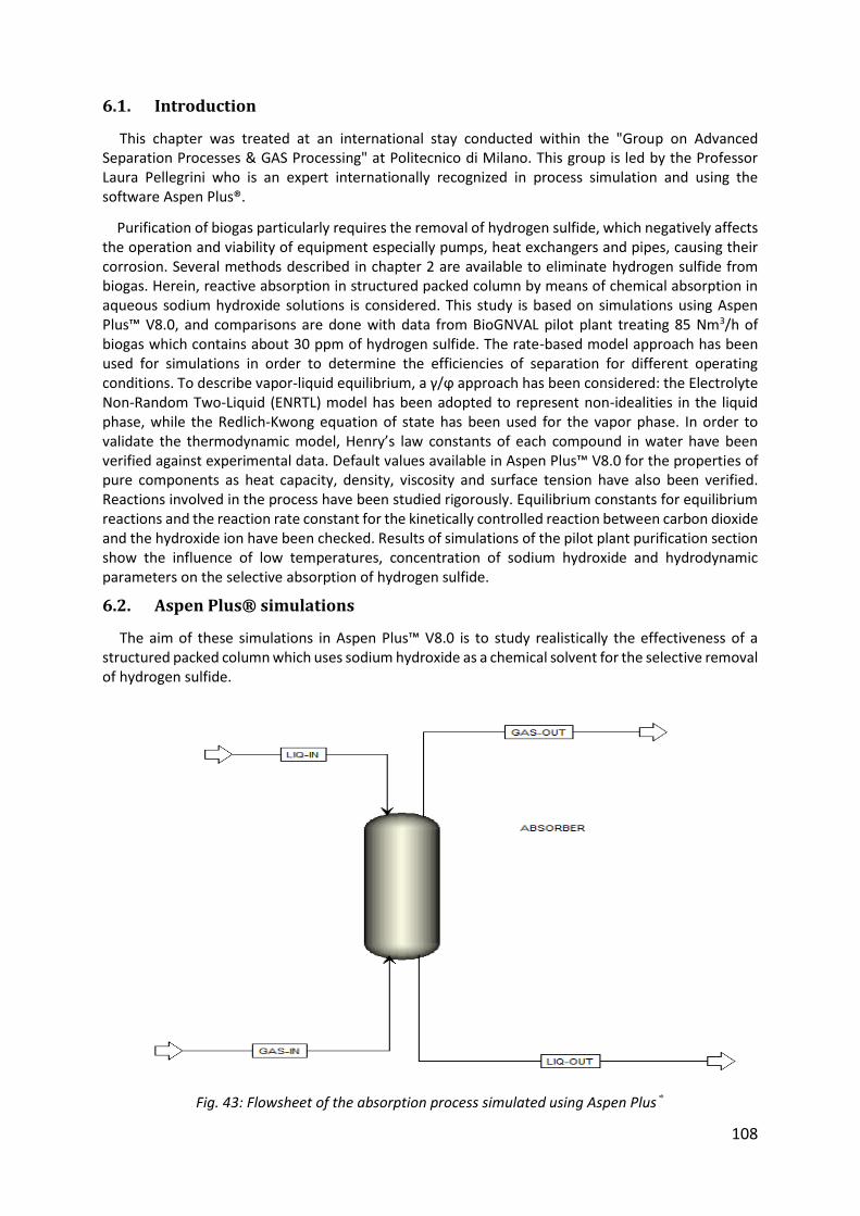
108
6.1. Introduction
This chapter was treated at an international stay conducted within the "Group on Advanced Separation Processes & GAS Processing" at Politecnico di Milano. This group is led by the Professor Laura Pellegrini who is an expert internationally recognized in process simulation and using the software Aspen Plus®.
Purification of biogas particularly requires the removal of hydrogen sulfide, which negatively affects the operation and viability of equipment especially pumps, heat exchangers and pipes, causing their corrosion. Several methods described in chapter 2 are available to eliminate hydrogen sulfide from biogas. Herein, reactive absorption in structured packed column by means of chemical absorption in aqueous sodium hydroxide solutions is considered. This study is based on simulations using Aspen Plus™ V8.0, and comparisons are done with data from BioGNVAL pilot plant treating 85 Nm3/h of biogas which contains about 30 ppm of hydrogen sulfide. The rate-based model approach has been used for simulations in order to determine the efficiencies of separation for different operating conditions. To describe vapor-liquid equilibrium, a γ/ϕ approach has been considered: the Electrolyte Non-Random Two-Liquid (ENRTL) model has been adopted to represent non-idealities in the liquid phase, while the Redlich-Kwong equation of state has been used for the vapor phase. In order to validate the thermodynamic model, Henry’s law constants of each compound in water have been verified against experimental data. Default values available in Aspen Plus™ V8.0 for the properties of pure components as heat capacity, density, viscosity and surface tension have also been verified. Reactions involved in the process have been studied rigorously. Equilibrium constants for equilibrium reactions and the reaction rate constant for the kinetically controlled reaction between carbon dioxide and the hydroxide ion have been checked. Results of simulations of the pilot plant purification section show the influence of low temperatures, concentration of sodium hydroxide and hydrodynamic parameters on the selective absorption of hydrogen sulfide.
6.2. Aspen Plus® simulations
The aim of these simulations in Aspen Plus™ V8.0 is to study realistically the effectiveness of a structured packed column which uses sodium hydroxide as a chemical solvent for the selective removal of hydrogen sulfide.
Fig. 43: Flowsheet of the absorption process simulated using Aspen Plus®

109
Unlike amines, sodium hydroxide is not regenerable but it is very effective in removing low contents of H2S [36].
Although the liquid solution is recycled, experimental data showed that the NaOH consumption is quite constant. NaOH concentration can be assumed to be constant over time in the liquid phase. This assumption justifies the use of the model "Rate-based" for the study.
The rate-based modeling approach is realistic compared to the traditional equilibrium-stage modeling approach that has been employed extensively in the process industries over the decades. The rate-based models assume that separation is caused by mass transfer between the contacting phases, and use the Maxwell-Stefan theory to calculate mass transfer rates [102]. Conversely, the equilibrium-stage models assume that the contacting phases are in equilibrium with
each other, which is an inherent approximation because the contacting phases are never in equilibrium
in a real column.
The rate-based modeling approach has many advantages over the equilibrium-stage modeling approach. The rate-based models represent a higher fidelity, more realistic modeling approach and the simulation results are more accurate than those attainable from the equilibrium-stage models [103].
The Electrolyte Non-Random Two-Liquid model proposed by Chen and Song [104] is used for
calculating the liquid phase properties, while the Redlich-Kwong equation of state is used to calculate
the vapor phase properties.
This model is verified and validated using various experimental data from literature.
6.2.1. Validation of the Temperature-Dependent Henry’s constant for CH4 – H2O, CO2 – H2O and H2S – H2O systems
For a rigorous estimation of gas solubility in the solvent, the Henry’s constants obtained with Aspen
Plus® should be verified by experimental data.
The Henry’s constants based on the mole fraction scale are taken from Aspen Plus® databanks for
the gaseous components (CH4, CO2 and H2S) with water.
The temperature dependence of the Henry’s constants used by Aspen Plus® is represented by:
ln 𝐻𝑖𝑗 = 𝑎𝑖𝑗 +𝑏𝑖𝑗
𝑇+ 𝑐𝑖𝑗 ln 𝑇 + 𝑑𝑖𝑗𝑇 +
𝑒𝑖𝑗
𝑇2 (83)
Coefficients aij, bij, cij, dij and eij are summarized in Table 45 for each system.
Table 45. Coefficients used by Aspen Plus® to calculate Henry’s constant
Component i CH4 CO2 H2S
Component j H2O H2O H2O
Low temperature [°C] 1.85 -0.15 -0.15
High temperature [°C] 79.85 226.85 149.85
aij 183.7811 159.1997 346.625
bij -9111.67 -8477.711 -13236.8
cij -25.0379 -21.957 -55.0551
dij 0.0001434 0.00578 0.05957
eij 0 0 0
Henry’s constants obtained with Aspen Plus® were compared to experimental data from the research report RR-48 of the Gas processors Association [105]. Results of Henry’s constants were also compared to the semi-empirical Equation (84) proposed by Harvey [106].
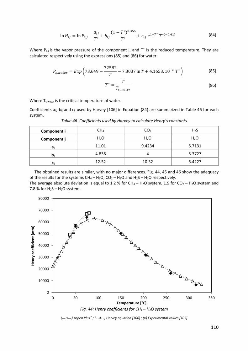
110
ln 𝐻𝑖𝑗 = ln 𝑃𝑠,𝑗 −𝑎𝑖𝑗
𝑇∗+ 𝑏𝑖𝑗
(1 − 𝑇∗)0.355
𝑇∗+ 𝑐𝑖𝑗 𝑒1−𝑇∗
𝑇∗(−0.41) (84)
Where Ps,j is the vapor pressure of the component j, and T* is the reduced temperature. They are
calculated respectively using the expressions (85) and (86) for water.
𝑃𝑠,𝑤𝑎𝑡𝑒𝑟 = 𝐸𝑥𝑝 (73.649 −72582
𝑇− 7.3037 ln 𝑇 + 4.1653. 10−6 𝑇2) (85)
𝑇∗ =𝑇
𝑇𝑐,𝑤𝑎𝑡𝑒𝑟 (86)
Where Tc,water is the critical temperature of water.
Coefficients aij, bij and cij used by Harvey [106] in Equation (84) are summarized in Table 46 for each system.
Table 46. Coefficients used by Harvey to calculate Henry’s constants
Component i CH4 CO2 H2S
Component j H2O H2O H2O
aij 11.01 9.4234 5.7131
bij 4.836 4 5.3727
cij 12.52 10.32 5.4227
The obtained results are similar, with no major differences. Fig. 44, 45 and 46 show the adequacy of the results for the systems CH4 – H2O, CO2 – H2O and H2S – H2O respectively. The average absolute deviation is equal to 1.2 % for CH4 – H2O system, 1.9 for CO2 – H2O system and 7.8 % for H2S – H2O system.
Fig. 44: Henry coefficients for CH4 – H2O system
(__□__) Aspen Plus® ; (- -Δ- -) Harvey equation [106] ; (♦) Experimental values [105]
0
10000
20000
30000
40000
50000
60000
70000
80000
0 50 100 150 200 250 300 350
He
nry
co
eff
icie
nt
[atm
]
Temperature [°C]
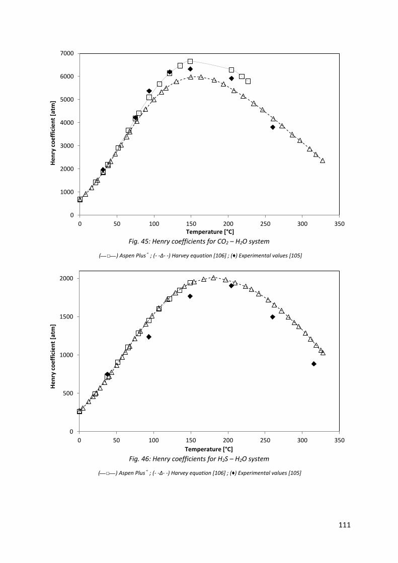
111
Fig. 45: Henry coefficients for CO2 – H2O system
(__□__) Aspen Plus® ; (- -Δ- -) Harvey equation [106] ; (♦) Experimental values [105]
Fig. 46: Henry coefficients for H2S – H2O system
(__□__) Aspen Plus® ; (- -Δ- -) Harvey equation [106] ; (♦) Experimental values [105]
0
1000
2000
3000
4000
5000
6000
7000
0 50 100 150 200 250 300 350
He
nry
co
eff
icie
nt
[atm
]
Temperature [°C]
0
500
1000
1500
2000
0 50 100 150 200 250 300 350
He
nry
co
eff
icie
nt
[atm
]
Temperature [°C]
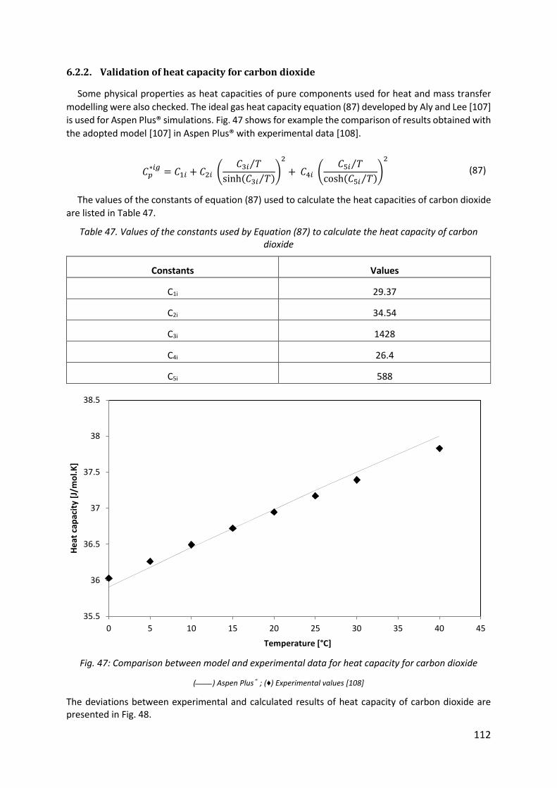
112
6.2.2. Validation of heat capacity for carbon dioxide
Some physical properties as heat capacities of pure components used for heat and mass transfer
modelling were also checked. The ideal gas heat capacity equation (87) developed by Aly and Lee [107]
is used for Aspen Plus® simulations. Fig. 47 shows for example the comparison of results obtained with
the adopted model [107] in Aspen Plus® with experimental data [108].
𝐶𝑝∗𝑖𝑔
= 𝐶1𝑖 + 𝐶2𝑖 (𝐶3𝑖 𝑇⁄
sinh(𝐶3𝑖 𝑇⁄ ))
2
+ 𝐶4𝑖 (𝐶5𝑖 𝑇⁄
cosh(𝐶5𝑖 𝑇⁄ ))
2
(87)
The values of the constants of equation (87) used to calculate the heat capacities of carbon dioxide
are listed in Table 47.
Table 47. Values of the constants used by Equation (87) to calculate the heat capacity of carbon dioxide
Constants Values
C1i 29.37
C2i 34.54
C3i 1428
C4i 26.4
C5i 588
Fig. 47: Comparison between model and experimental data for heat capacity for carbon dioxide
(____) Aspen Plus® ; (♦) Experimental values [108]
The deviations between experimental and calculated results of heat capacity of carbon dioxide are presented in Fig. 48.
35.5
36
36.5
37
37.5
38
38.5
0 5 10 15 20 25 30 35 40 45
He
at c
apac
ity
[J/m
ol.
K]
Temperature [°C]
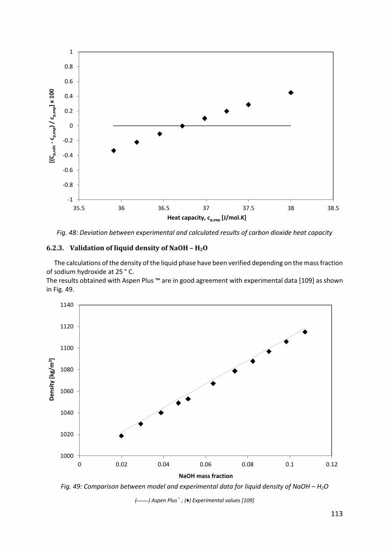
113
Fig. 48: Deviation between experimental and calculated results of carbon dioxide heat capacity
6.2.3. Validation of liquid density of NaOH – H2O
The calculations of the density of the liquid phase have been verified depending on the mass fraction of sodium hydroxide at 25 ° C. The results obtained with Aspen Plus ™ are in good agreement with experimental data [109] as shown in Fig. 49.
Fig. 49: Comparison between model and experimental data for liquid density of NaOH – H2O
(____) Aspen Plus® ; (♦) Experimental values [109]
-1
-0.8
-0.6
-0.4
-0.2
0
0.2
0.4
0.6
0.8
1
35.5 36 36.5 37 37.5 38 38.5
[(C
p,c
alc
-c p
,exp
) /
c p,e
xp]
x 1
00
Heat capacity, cp,exp [J/mol.K]
1000
1020
1040
1060
1080
1100
1120
1140
0 0.02 0.04 0.06 0.08 0.1 0.12
De
nsi
ty [
kg/m
3 ]
NaOH mass fraction
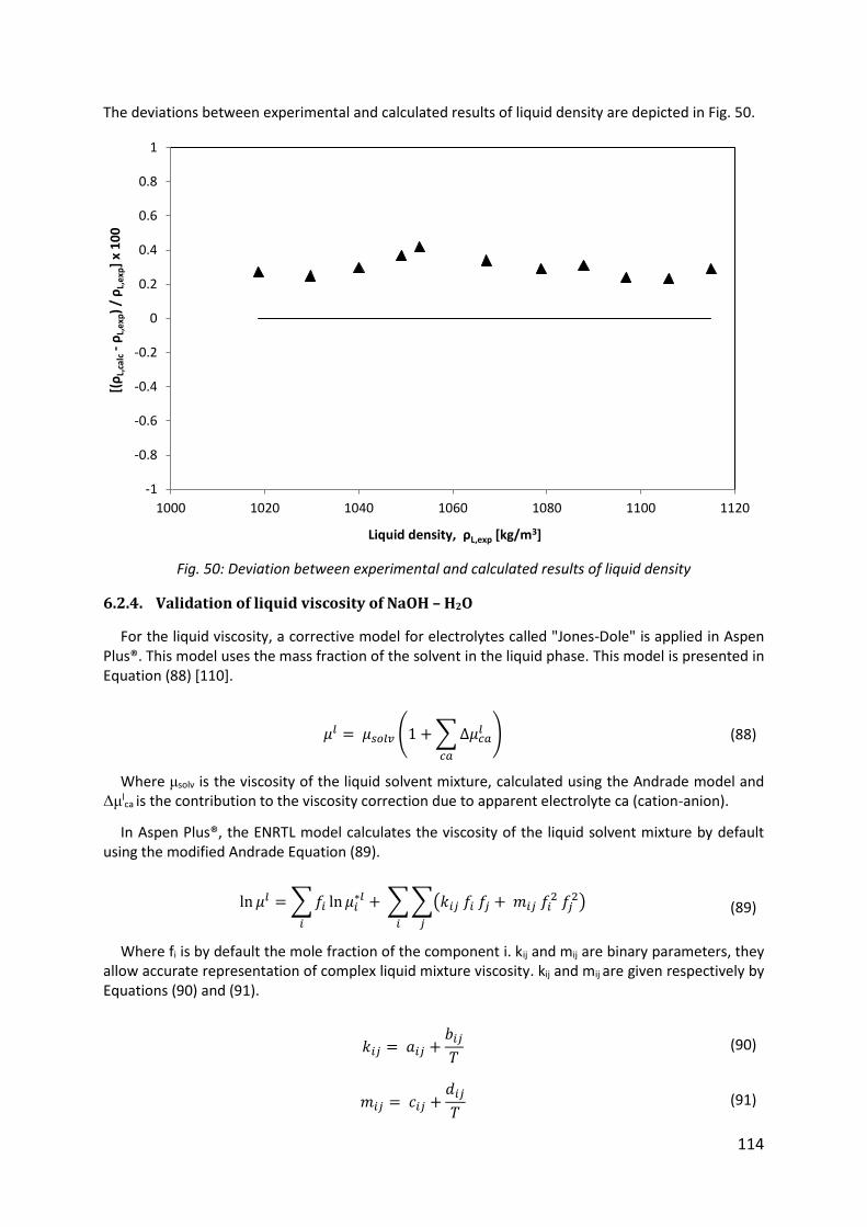
114
The deviations between experimental and calculated results of liquid density are depicted in Fig. 50.
Fig. 50: Deviation between experimental and calculated results of liquid density
6.2.4. Validation of liquid viscosity of NaOH – H2O
For the liquid viscosity, a corrective model for electrolytes called "Jones-Dole" is applied in Aspen Plus®. This model uses the mass fraction of the solvent in the liquid phase. This model is presented in Equation (88) [110].
𝜇𝑙 = 𝜇𝑠𝑜𝑙𝑣 (1 + ∑ ∆𝜇𝑐𝑎𝑙
𝑐𝑎
) (88)
Where μsolv is the viscosity of the liquid solvent mixture, calculated using the Andrade model and Δμl
ca is the contribution to the viscosity correction due to apparent electrolyte ca (cation-anion).
In Aspen Plus®, the ENRTL model calculates the viscosity of the liquid solvent mixture by default using the modified Andrade Equation (89).
ln 𝜇𝑙 = ∑ 𝑓𝑖 ln 𝜇𝑖∗𝑙 + ∑ ∑(𝑘𝑖𝑗 𝑓𝑖 𝑓𝑗 + 𝑚𝑖𝑗 𝑓𝑖
2 𝑓𝑗2)
𝑗𝑖𝑖
(89)
Where fi is by default the mole fraction of the component i. kij and mij are binary parameters, they allow accurate representation of complex liquid mixture viscosity. kij and mij are given respectively by Equations (90) and (91).
𝑘𝑖𝑗 = 𝑎𝑖𝑗 +𝑏𝑖𝑗
𝑇 (90)
𝑚𝑖𝑗 = 𝑐𝑖𝑗 +𝑑𝑖𝑗
𝑇 (91)
-1
-0.8
-0.6
-0.4
-0.2
0
0.2
0.4
0.6
0.8
1
1000 1020 1040 1060 1080 1100 1120
[(ρ
L,ca
lc-
ρL,
exp
) /
ρL,
exp
] x
10
0
Liquid density, ρL,exp [kg/m3]
115
When the electrolyte concentration exceeds 0.1 M, Aspen Plus® uses the Equation (92) of Breslau and Miller instead of that of Jones and Dole [111].
∆𝜇𝑐𝑎𝑙 = 2.5 𝑉𝑒 𝑐𝑐𝑎
𝑎 + 10.05 𝑉𝑒(𝑐𝑐𝑎𝑎 )2 (92)
Where Ve is the effective volume. It is given by Equation (92).
𝑉𝑒 =𝐵𝑐𝑎−0.002
2.6 For salts involving univalent ions (93.a)
𝑉𝑒 =𝐵𝑐𝑎−0.011
5.06 For other salts (93.b)
Where Bca is calculated using Equation (94).
𝐵𝑐𝑎 = (𝑏𝑐,1 + 𝑏𝑐,2 𝑇) + (𝑏𝑎,1 + 𝑏𝑎,2 𝑇) (94)
caca is the concentration of apparent electrolyte ca. It is calculated using Equation (95).
𝑐𝑐𝑎𝑎 =
𝑥𝑐𝑎𝑎
𝑉𝑚𝑙
(95)
Where xaca is the mole fraction of the apparent electrolyte ca and Vl
m is the molar volume of the liquid mixture calculated by the Clarke model.
The electrolyte correction model parameters were improved for the ion HCO3- using KHCO3 - H2O viscosity data [112]. The regression of parameters for Na+ ion was performed with viscosity data of NaOH – H2O system [113]. For ion CO3
2-, parameters have been optimized considering experimental data for the K2CO3 - H2O system [114]. For other ions, values provided by Aspen Plus® database were used.
Fig. 51 shows the fit between experimental data and Aspen Plus® results for the viscosity of the liquid phase as a function of the mass fraction of sodium hydroxide. Data of this comparison are carried out at a temperature of about 25 °C.
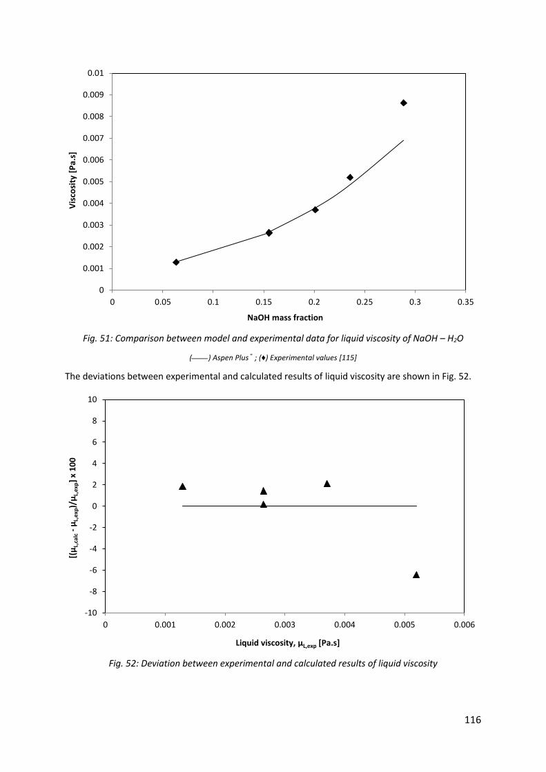
116
Fig. 51: Comparison between model and experimental data for liquid viscosity of NaOH – H2O
(____) Aspen Plus® ; (♦) Experimental values [115]
The deviations between experimental and calculated results of liquid viscosity are shown in Fig. 52.
Fig. 52: Deviation between experimental and calculated results of liquid viscosity
0
0.001
0.002
0.003
0.004
0.005
0.006
0.007
0.008
0.009
0.01
0 0.05 0.1 0.15 0.2 0.25 0.3 0.35
Vis
cosi
ty [
Pa.
s]
NaOH mass fraction
-10
-8
-6
-4
-2
0
2
4
6
8
10
0 0.001 0.002 0.003 0.004 0.005 0.006
[(μ
L,ca
lc-
μL,
exp)/
μL,
exp]
x 1
00
Liquid viscosity, μL,exp [Pa.s]

117
6.2.5. Validation of surface tension of NaOH – H2O
To calculate the liquid phase surface tension, Aspen Plus® uses the model of Onsager-Samaras presented by Equation (96). Results obtained were compared to experimental data found in literature, as shown in Fig. 53 [116].
𝜎 = 𝜎𝑠𝑜𝑙𝑣 + ∑ 𝑥𝑐𝑎𝑎
𝑐𝑎
∆𝜎𝑐𝑎 (96)
Where σsolv is the surface tension of the solvent mixture calculated using the General Pure Component Liquid Surface Tension Model [117] and Δσca is the contribution to the surface tension correction due to apparent electrolyte ca, calculated using Equation (97).
∆𝜎𝑐𝑎 =80
휀𝑠𝑜𝑙𝑣 𝑐𝑐𝑎
𝑎 𝑙𝑜𝑔 [1.13 × 10⁻¹³ (휀𝑠𝑜𝑙𝑣 𝑇)3
𝑐𝑐𝑎𝑎 ] (97)
Where ɛsolv is the dielectric constant of the solvent mixture.
Fig. 53: Comparison between model and experimental data for liquid phase surface tension of 5 wt% NaOH aqueous solution
(____) Aspen Plus® ; (♦) Experimental values [116]
The deviations between experimental and calculated results of surface tension are presented in Fig. 54.
0.064
0.066
0.068
0.07
0.072
0.074
0.076
0 10 20 30 40 50 60 70 80
Surf
ace
te
nsi
on
[N
/m]
Temperature [°C]
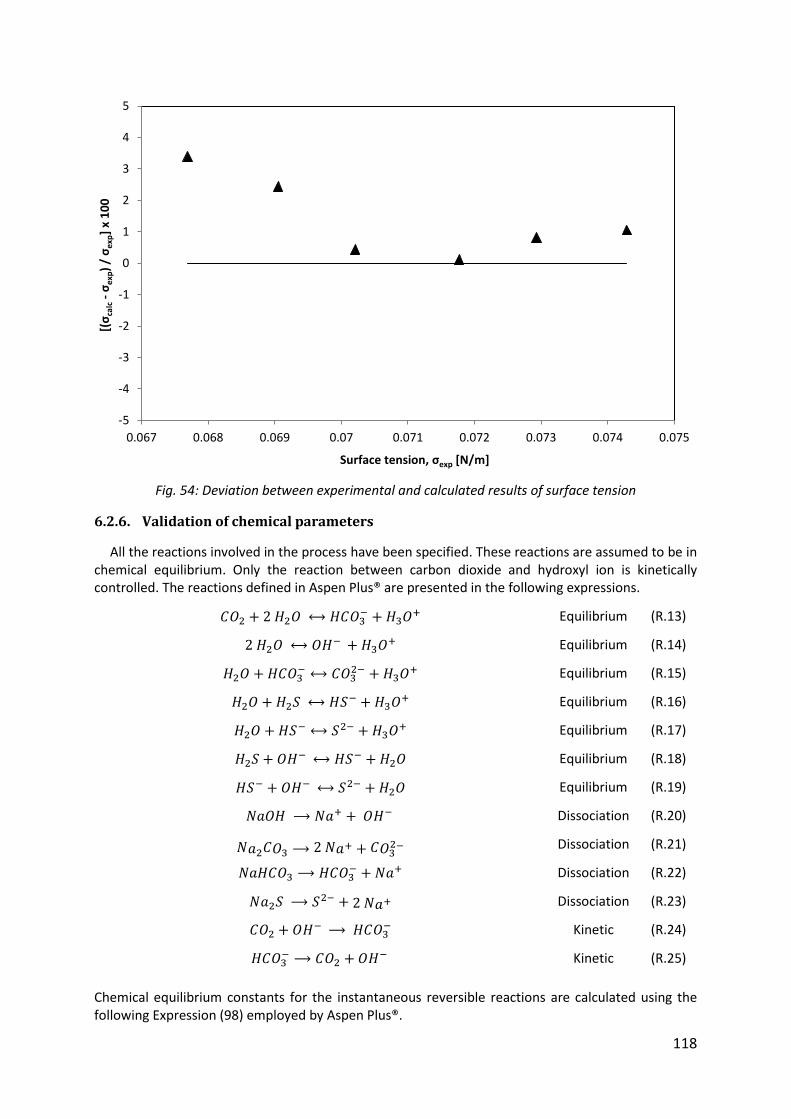
118
Fig. 54: Deviation between experimental and calculated results of surface tension
6.2.6. Validation of chemical parameters
All the reactions involved in the process have been specified. These reactions are assumed to be in chemical equilibrium. Only the reaction between carbon dioxide and hydroxyl ion is kinetically controlled. The reactions defined in Aspen Plus® are presented in the following expressions.
𝐶𝑂2 + 2 𝐻2𝑂 ⟷ 𝐻𝐶𝑂3− + 𝐻3𝑂+ Equilibrium (R.13)
2 𝐻2𝑂 ⟷ 𝑂𝐻− + 𝐻3𝑂+ Equilibrium (R.14)
𝐻2𝑂 + 𝐻𝐶𝑂3− ⟷ 𝐶𝑂3
2− + 𝐻3𝑂+ Equilibrium (R.15)
𝐻2𝑂 + 𝐻2𝑆 ⟷ 𝐻𝑆− + 𝐻3𝑂+ Equilibrium (R.16)
𝐻2𝑂 + 𝐻𝑆− ⟷ 𝑆2− + 𝐻3𝑂+ Equilibrium (R.17)
𝐻2𝑆 + 𝑂𝐻− ⟷ 𝐻𝑆− + 𝐻2𝑂 Equilibrium (R.18)
𝐻𝑆− + 𝑂𝐻− ⟷ 𝑆2− + 𝐻2𝑂 Equilibrium (R.19)
𝑁𝑎𝑂𝐻 ⟶ 𝑁𝑎+ + 𝑂𝐻− Dissociation (R.20)
𝑁𝑎2𝐶𝑂3 ⟶ 2 𝑁𝑎+ + 𝐶𝑂32− Dissociation (R.21)
𝑁𝑎𝐻𝐶𝑂3 ⟶ 𝐻𝐶𝑂3− + 𝑁𝑎+ Dissociation (R.22)
𝑁𝑎2𝑆 ⟶ 𝑆2− + 2 𝑁𝑎+ Dissociation (R.23)
𝐶𝑂2 + 𝑂𝐻− ⟶ 𝐻𝐶𝑂3− Kinetic (R.24)
𝐻𝐶𝑂3− ⟶ 𝐶𝑂2 + 𝑂𝐻− Kinetic (R.25)
Chemical equilibrium constants for the instantaneous reversible reactions are calculated using the following Expression (98) employed by Aspen Plus®.
-5
-4
-3
-2
-1
0
1
2
3
4
5
0.067 0.068 0.069 0.07 0.071 0.072 0.073 0.074 0.075
[(σ
calc
-σ
exp
) /
σe
xp]
x 1
00
Surface tension, σexp [N/m]
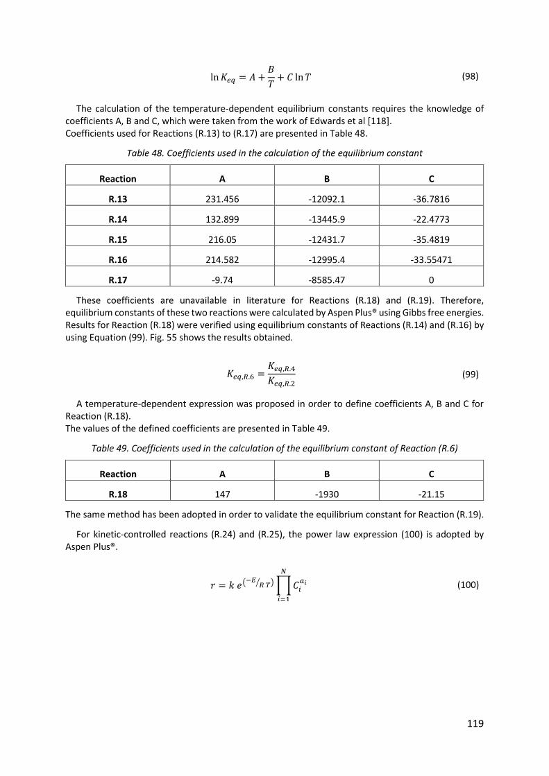
119
ln 𝐾𝑒𝑞 = 𝐴 +𝐵
𝑇+ 𝐶 ln 𝑇 (98)
The calculation of the temperature-dependent equilibrium constants requires the knowledge of coefficients A, B and C, which were taken from the work of Edwards et al [118]. Coefficients used for Reactions (R.13) to (R.17) are presented in Table 48.
Table 48. Coefficients used in the calculation of the equilibrium constant
Reaction A B C
R.13 231.456 -12092.1 -36.7816
R.14 132.899 -13445.9 -22.4773
R.15 216.05 -12431.7 -35.4819
R.16 214.582 -12995.4 -33.55471
R.17 -9.74 -8585.47 0
These coefficients are unavailable in literature for Reactions (R.18) and (R.19). Therefore, equilibrium constants of these two reactions were calculated by Aspen Plus® using Gibbs free energies. Results for Reaction (R.18) were verified using equilibrium constants of Reactions (R.14) and (R.16) by using Equation (99). Fig. 55 shows the results obtained.
𝐾𝑒𝑞,𝑅.6 =𝐾𝑒𝑞,𝑅.4
𝐾𝑒𝑞,𝑅.2 (99)
A temperature-dependent expression was proposed in order to define coefficients A, B and C for Reaction (R.18). The values of the defined coefficients are presented in Table 49.
Table 49. Coefficients used in the calculation of the equilibrium constant of Reaction (R.6)
Reaction A B C
R.18 147 -1930 -21.15
The same method has been adopted in order to validate the equilibrium constant for Reaction (R.19).
For kinetic-controlled reactions (R.24) and (R.25), the power law expression (100) is adopted by Aspen Plus®.
𝑟 = 𝑘 𝑒(−𝐸𝑅 𝑇⁄ ) ∏ 𝐶𝑖
𝑎𝑖
𝑁
𝑖=1
(100)
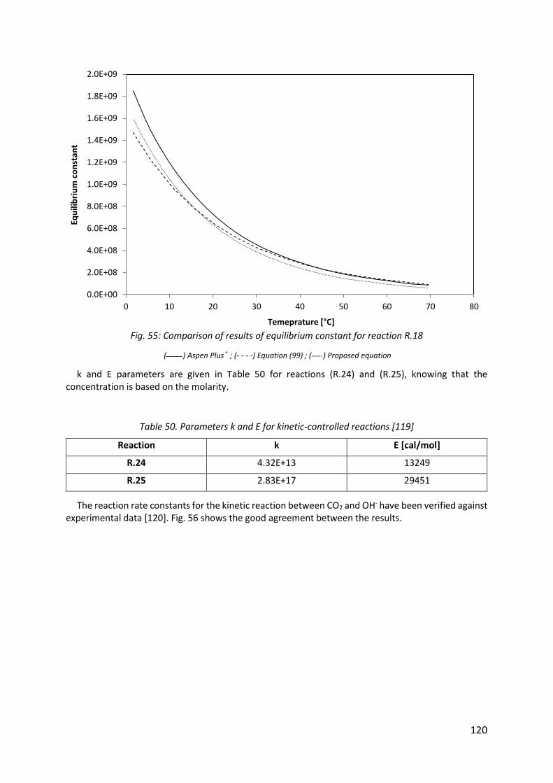
120
Fig. 55: Comparison of results of equilibrium constant for reaction R.18
(____) Aspen Plus® ; (- - - -) Equation (99) ; (……) Proposed equation
k and E parameters are given in Table 50 for reactions (R.24) and (R.25), knowing that the concentration is based on the molarity.
Table 50. Parameters k and E for kinetic-controlled reactions [119]
Reaction k E [cal/mol]
R.24 4.32E+13 13249
R.25 2.83E+17 29451
The reaction rate constants for the kinetic reaction between CO2 and OH- have been verified against experimental data [120]. Fig. 56 shows the good agreement between the results.
0.0E+00
2.0E+08
4.0E+08
6.0E+08
8.0E+08
1.0E+09
1.2E+09
1.4E+09
1.6E+09
1.8E+09
2.0E+09
0 10 20 30 40 50 60 70 80
Equ
ilib
riu
m c
on
stan
t
Temeprature [°C]
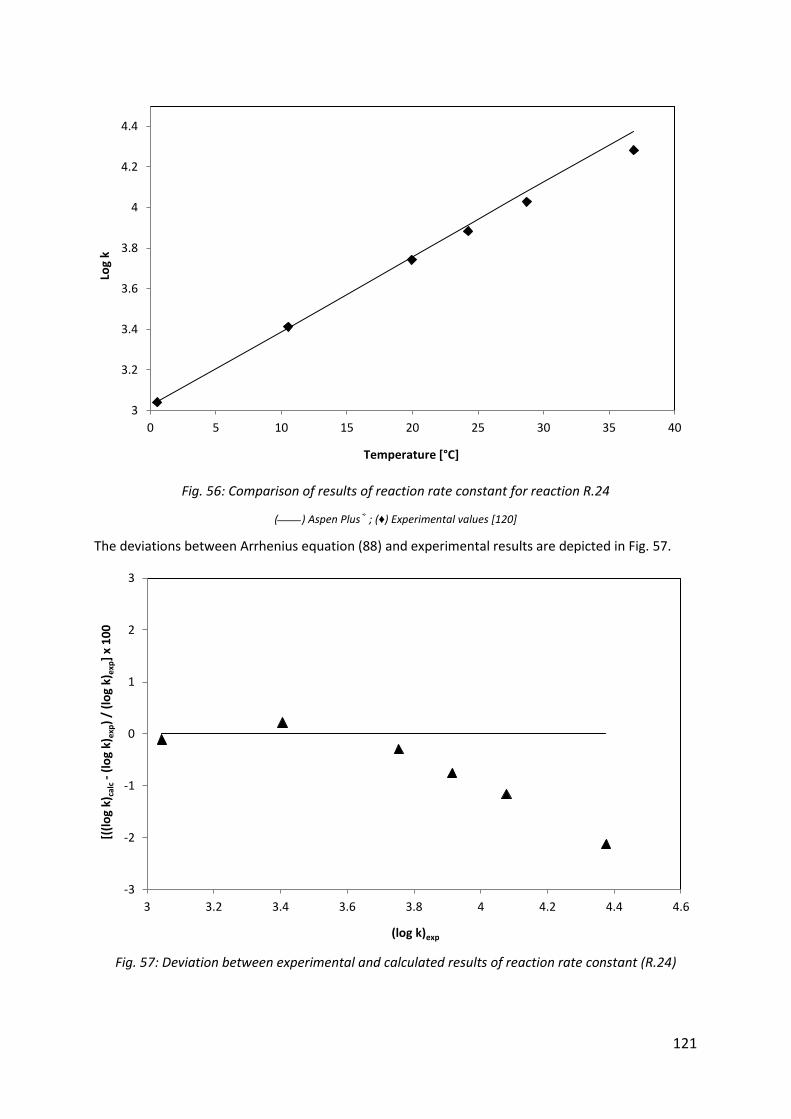
121
Fig. 56: Comparison of results of reaction rate constant for reaction R.24
(____) Aspen Plus® ; (♦) Experimental values [120]
The deviations between Arrhenius equation (88) and experimental results are depicted in Fig. 57.
Fig. 57: Deviation between experimental and calculated results of reaction rate constant (R.24)
3
3.2
3.4
3.6
3.8
4
4.2
4.4
0 5 10 15 20 25 30 35 40
Log
k
Temperature [°C]
-3
-2
-1
0
1
2
3
3 3.2 3.4 3.6 3.8 4 4.2 4.4 4.6
[((l
og
k)ca
lc-
(lo
g k)
exp)
/ (l
og
k)ex
p]
x 1
00
(log k)exp
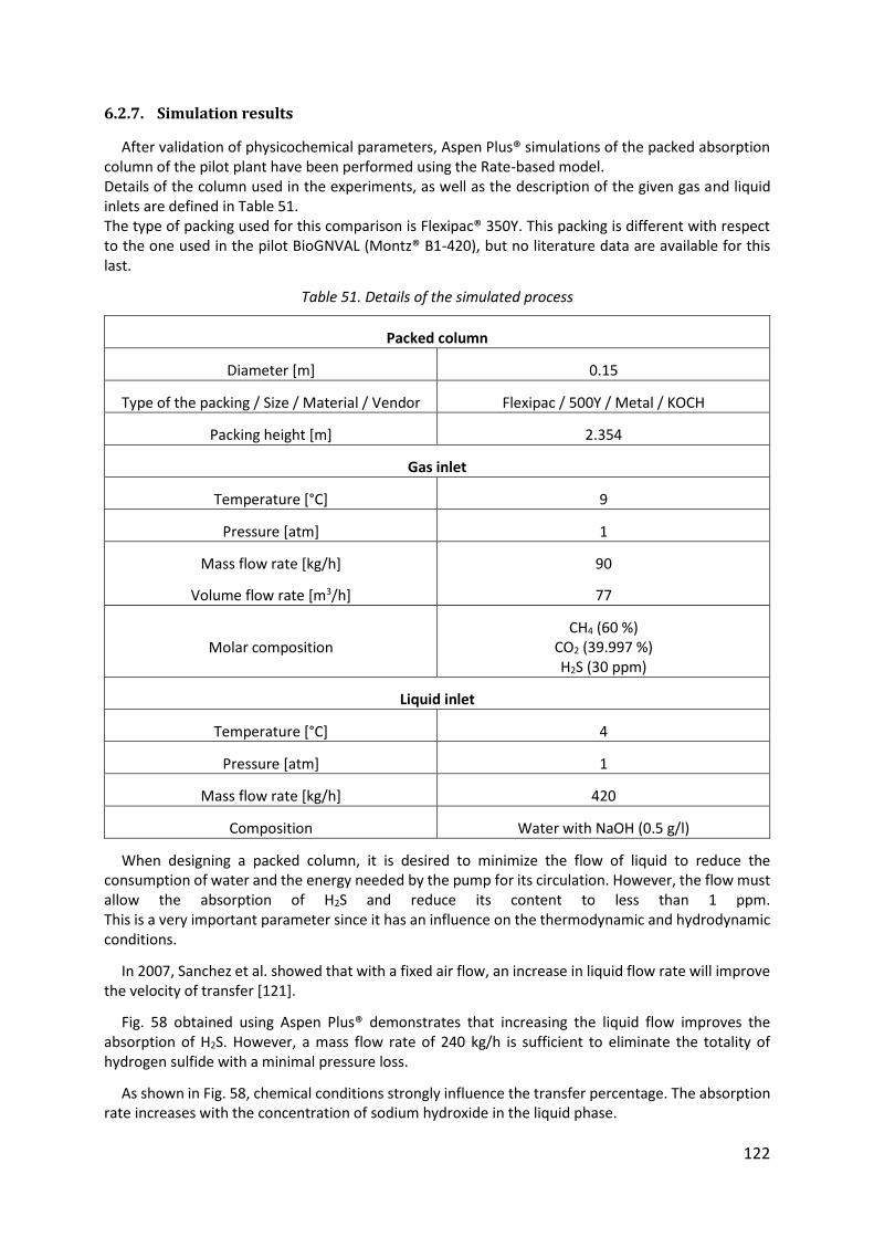
122
6.2.7. Simulation results
After validation of physicochemical parameters, Aspen Plus® simulations of the packed absorption column of the pilot plant have been performed using the Rate-based model. Details of the column used in the experiments, as well as the description of the given gas and liquid inlets are defined in Table 51. The type of packing used for this comparison is Flexipac® 350Y. This packing is different with respect to the one used in the pilot BioGNVAL (Montz® B1-420), but no literature data are available for this last.
Table 51. Details of the simulated process
Packed column
Diameter [m] 0.15
Type of the packing / Size / Material / Vendor Flexipac / 500Y / Metal / KOCH
Packing height [m] 2.354
Gas inlet
Temperature [°C] 9
Pressure [atm] 1
Mass flow rate [kg/h]
Volume flow rate [m3/h]
90
77
Molar composition CH4 (60 %)
CO2 (39.997 %) H2S (30 ppm)
Liquid inlet
Temperature [°C] 4
Pressure [atm] 1
Mass flow rate [kg/h] 420
Composition Water with NaOH (0.5 g/l)
When designing a packed column, it is desired to minimize the flow of liquid to reduce the consumption of water and the energy needed by the pump for its circulation. However, the flow must allow the absorption of H2S and reduce its content to less than 1 ppm. This is a very important parameter since it has an influence on the thermodynamic and hydrodynamic conditions.
In 2007, Sanchez et al. showed that with a fixed air flow, an increase in liquid flow rate will improve the velocity of transfer [121].
Fig. 58 obtained using Aspen Plus® demonstrates that increasing the liquid flow improves the absorption of H2S. However, a mass flow rate of 240 kg/h is sufficient to eliminate the totality of hydrogen sulfide with a minimal pressure loss.
As shown in Fig. 58, chemical conditions strongly influence the transfer percentage. The absorption rate increases with the concentration of sodium hydroxide in the liquid phase.
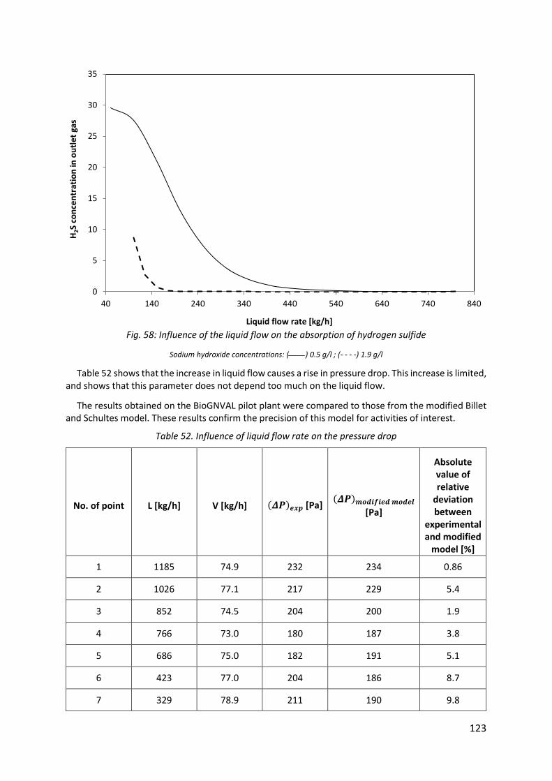
123
Fig. 58: Influence of the liquid flow on the absorption of hydrogen sulfide
Sodium hydroxide concentrations: (____) 0.5 g/l ; (- - - -) 1.9 g/l
Table 52 shows that the increase in liquid flow causes a rise in pressure drop. This increase is limited, and shows that this parameter does not depend too much on the liquid flow.
The results obtained on the BioGNVAL pilot plant were compared to those from the modified Billet and Schultes model. These results confirm the precision of this model for activities of interest.
Table 52. Influence of liquid flow rate on the pressure drop
No. of point L [kg/h] V [kg/h] (𝜟𝑷)𝒆𝒙𝒑 [Pa] (𝜟𝑷)𝒎𝒐𝒅𝒊𝒇𝒊𝒆𝒅 𝒎𝒐𝒅𝒆𝒍
[Pa]
Absolute value of relative
deviation between
experimental and modified
model [%]
1 1185 74.9 232 234 0.86
2 1026 77.1 217 229 5.4
3 852 74.5 204 200 1.9
4 766 73.0 180 187 3.8
5 686 75.0 182 191 5.1
6 423 77.0 204 186 8.7
7 329 78.9 211 190 9.8
0
5
10
15
20
25
30
35
40 140 240 340 440 540 640 740 840
H2S
co
nce
ntr
atio
n in
ou
tle
t ga
s
Liquid flow rate [kg/h]

124
The dependence between the pressure drop and the gas flow rate is much more important as shown in Fig. 59, because the gas has the continuous phase in the packed column.
Fig. 59: Influence of gas flow rate on the pressure drop
(____) Modified Billet and Schultes model ; (♦) Experimental values [BioGNVAL, 2015]
The deviations between experimental and calculated results of pressure drop are presented in Fig. 60.
Fig. 60: Deviation between experimental and calculated results of pressure drop
160
210
260
310
360
410
460
63 68 73 78 83 88 93
Pre
ssu
re d
rop
[P
a]
Gas flow rate [m3/h]
-12
-7
-2
3
8
175 195 215 235 255 275 295 315 335 355
[(Δ
Pca
lc-
ΔP
exp)
/ Δ
Pex
p]
x 1
00
Pressure drop, ΔPexp [Pa]
125
When hydrogen sulfide is absorbed into a sodium hydroxide solution, it can react directly with hydroxyl ions by a proton transfer reaction as seen in Reaction R.18. Compared to the diffusion phenomena, this reaction is extremely rapid and can be considered instantaneous. Since hydrogen sulfide is absorbed more rapidly than carbon dioxide by aqueous sodium hydroxide solutions, partial selectivity can be attained when both gases are present as seen in Fig. 61. Selectivity is favored by short gas-liquid contact times and low temperatures [36].
Fig. 61: Influence of the concentration of NaOH in the removal of H2S and CO2
Compound: (____) CO2 ; (- - - -) H2S
A key parameter affecting the overall performances of the absorption unit is the temperature, since it affects physicochemical properties (such as the solubility of acidic compounds in the aqueous phase, according to the Henry’s law) and the chemical reactions in the liquid phase. Fig. 62 shows a good agreement between the results of Aspen Plus® simulations and those obtained from the pilot plant.
0
5
10
15
20
25
30
35
40
0
2
4
6
8
10
12
14
16
18
20
0 0.2 0.4 0.6 0.8 1 1.2
Mo
lar
pe
rce
nta
ge o
f C
O2
in o
utl
et
gas
[%]
H2S
con
cen
trat
ion
in o
utl
et
gas
[pp
m]
NaOH concentration [g/l]
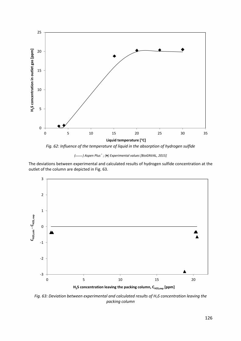
126
Fig. 62: Influence of the temperature of liquid in the absorption of hydrogen sulfide
(____) Aspen Plus® ; (♦) Experimental values [BioGNVAL, 2015]
The deviations between experimental and calculated results of hydrogen sulfide concentration at the outlet of the column are depicted in Fig. 63.
Fig. 63: Deviation between experimental and calculated results of H2S concentration leaving the packing column
0
5
10
15
20
25
0 5 10 15 20 25 30 35
H2S
co
nce
ntr
atio
n in
ou
tle
t ga
s [p
pm
]
Liquid temperature [°C]
-3
-2
-1
0
1
2
3
0 5 10 15 20
CH
2S,c
alc
-C
H2S
, exp
H2S concentration leaving the packing column, CH2S,exp [ppm]
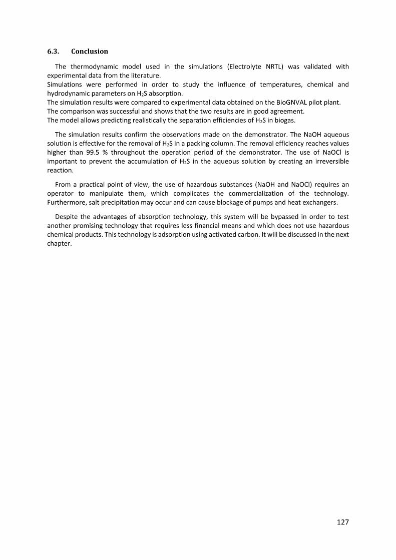
127
6.3. Conclusion
The thermodynamic model used in the simulations (Electrolyte NRTL) was validated with experimental data from the literature. Simulations were performed in order to study the influence of temperatures, chemical and hydrodynamic parameters on H2S absorption. The simulation results were compared to experimental data obtained on the BioGNVAL pilot plant. The comparison was successful and shows that the two results are in good agreement. The model allows predicting realistically the separation efficiencies of H2S in biogas.
The simulation results confirm the observations made on the demonstrator. The NaOH aqueous solution is effective for the removal of H2S in a packing column. The removal efficiency reaches values higher than 99.5 % throughout the operation period of the demonstrator. The use of NaOCl is important to prevent the accumulation of H2S in the aqueous solution by creating an irreversible reaction.
From a practical point of view, the use of hazardous substances (NaOH and NaOCl) requires an operator to manipulate them, which complicates the commercialization of the technology. Furthermore, salt precipitation may occur and can cause blockage of pumps and heat exchangers.
Despite the advantages of absorption technology, this system will be bypassed in order to test another promising technology that requires less financial means and which does not use hazardous chemical products. This technology is adsorption using activated carbon. It will be discussed in the next chapter.
128
Chapter 7: Modeling hydrogen sulfide adsorption onto activated carbon
Résumé :
Le dernier chapitre concerne la modélisation du procédé d’adsorption du H2S sur charbon actif. Un modèle dynamique a été développé pour modéliser la courbe de percée du système H2S – charbon actif.
La courbe de percée est utilisée pour décrire l'évolution spatio-temporelle de la concentration de H2S en phase gazeuse. Ce type de modélisation de la dynamique de la colonne d'adsorption est basé sur la définition des bilans de matière : un bilan de masse de la phase gazeuse où le transfert par convection domine et un bilan massique des particules adsorbantes où le transfert par diffusion domine.
Au cours de cette étude, les différents coefficients de transfert de masse impliqués dans le processus ont été estimés dans les mêmes conditions dans lesquelles les expérimentations sur le démonstrateur "BioGNVAL" ont eu lieu.
Les simulations ont été effectuées seulement pour des concentrations élevées en H2S car une unité d’adsorption industrielle qui traite de faibles concentrations en H2S atteint la saturation dans une période de quelques mois (≈ 3 mois). La simulation de cette période avec un pas de temps de 0,01 s exige des temps de calculs énormes qui ne sont pas supportés par la machine de travail. De plus, l'augmentation du pas de temps entraînera la divergence des calculs.
Les résultats obtenus avec le modèle développé devraient être comparés aux données expérimentales afin d'ajuster le coefficient global de transfert de masse et les paramètres d'équilibre donnés par l'isotherme d'adsorption.
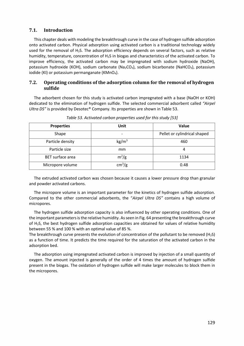
129
7.1. Introduction
This chapter deals with modeling the breakthrough curve in the case of hydrogen sulfide adsorption onto activated carbon. Physical adsorption using activated carbon is a traditional technology widely used for the removal of H2S. The adsorption efficiency depends on several factors, such as relative humidity, temperature, concentration of H2S in biogas and characteristics of the activated carbon. To improve efficiency, the activated carbon may be impregnated with sodium hydroxide (NaOH), potassium hydroxide (KOH), sodium carbonate (Na2CO3), sodium bicarbonate (NaHCO3), potassium iodide (KI) or potassium permanganate (KMnO4).
7.2. Operating conditions of the adsorption column for the removal of hydrogen sulfide
The adsorbent chosen for this study is activated carbon impregnated with a base (NaOH or KOH) dedicated to the elimination of hydrogen sulfide. The selected commercial adsorbent called “Airpel Ultra DS” is provided by Desotec® Company. Its properties are shown in Table 53.
Table 53. Activated carbon properties used for this study [53]
Properties Unit Value
Shape - Pellet or cylindrical shaped
Particle density kg/m3 460
Particle size mm 4
BET surface area m2/g 1134
Micropore volume cm3/g 0.48
The extruded activated carbon was chosen because it causes a lower pressure drop than granular
and powder activated carbons.
The micropore volume is an important parameter for the kinetics of hydrogen sulfide adsorption. Compared to the other commercial adsorbents, the “Airpel Ultra DS” contains a high volume of micropores.
The hydrogen sulfide adsorption capacity is also influenced by other operating conditions. One of the important parameters is the relative humidity. As seen in Fig. 64 presenting the breakthrough curve of H2S, the best hydrogen sulfide adsorption capacities are obtained for values of relative humidity between 55 % and 100 % with an optimal value of 85 %. The breakthrough curve presents the evolution of concentration of the pollutant to be removed (H2S) as a function of time. It predicts the time required for the saturation of the activated carbon in the adsorption bed.
The adsorption using impregnated activated carbon is improved by injection of a small quantity of oxygen. The amount injected is generally of the order of 4 times the amount of hydrogen sulfide present in the biogas. The oxidation of hydrogen sulfide will make larger molecules to block them in the micropores.

130
Fig. 64: Influence of relative humidity in the adsorption of hydrogen sulfide using Airpel Ultra DS [53]
Relative humidity: (……) 0 % ; (− .. − ..) 33 % ; (- - - -) 58 % ; (− . − . −) 85 % ; (____) 100 %
0
200
400
600
800
1000
1200
0 10 20 30 40 50 60
Bre
akth
rou
gh H
2S [
pp
m]
Breakthrough time [h]
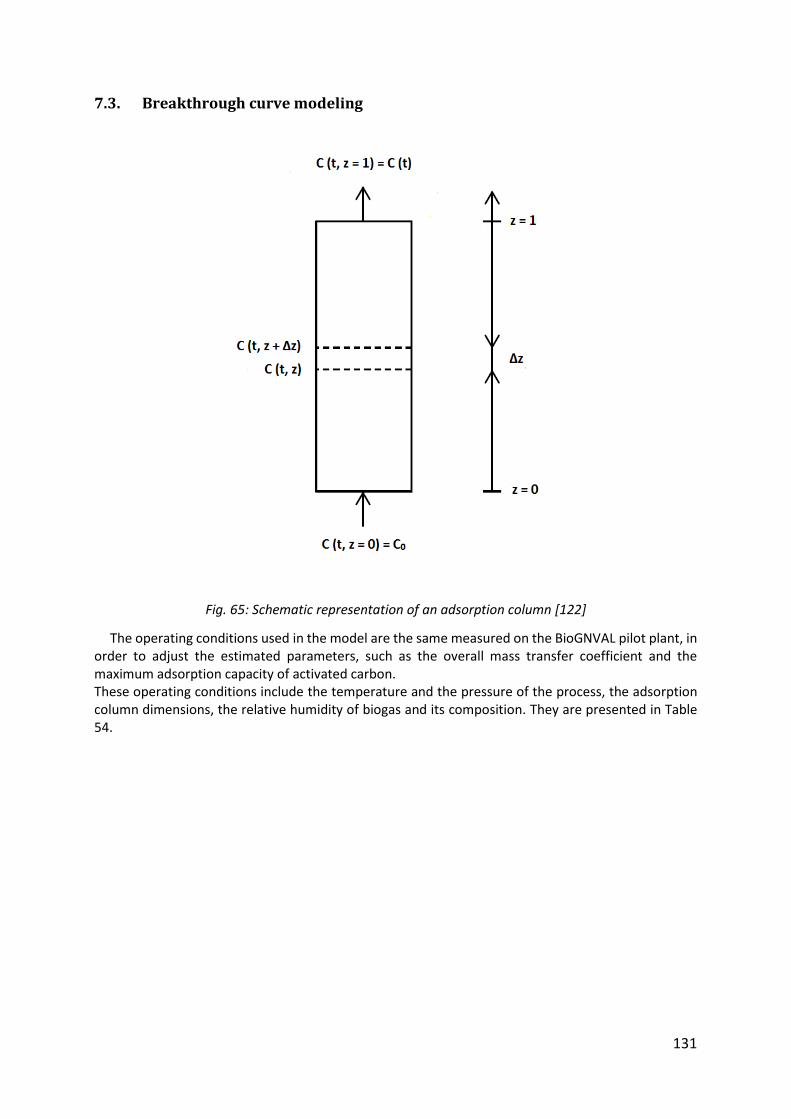
131
7.3. Breakthrough curve modeling
Fig. 65: Schematic representation of an adsorption column [122]
The operating conditions used in the model are the same measured on the BioGNVAL pilot plant, in order to adjust the estimated parameters, such as the overall mass transfer coefficient and the maximum adsorption capacity of activated carbon. These operating conditions include the temperature and the pressure of the process, the adsorption column dimensions, the relative humidity of biogas and its composition. They are presented in Table 54.
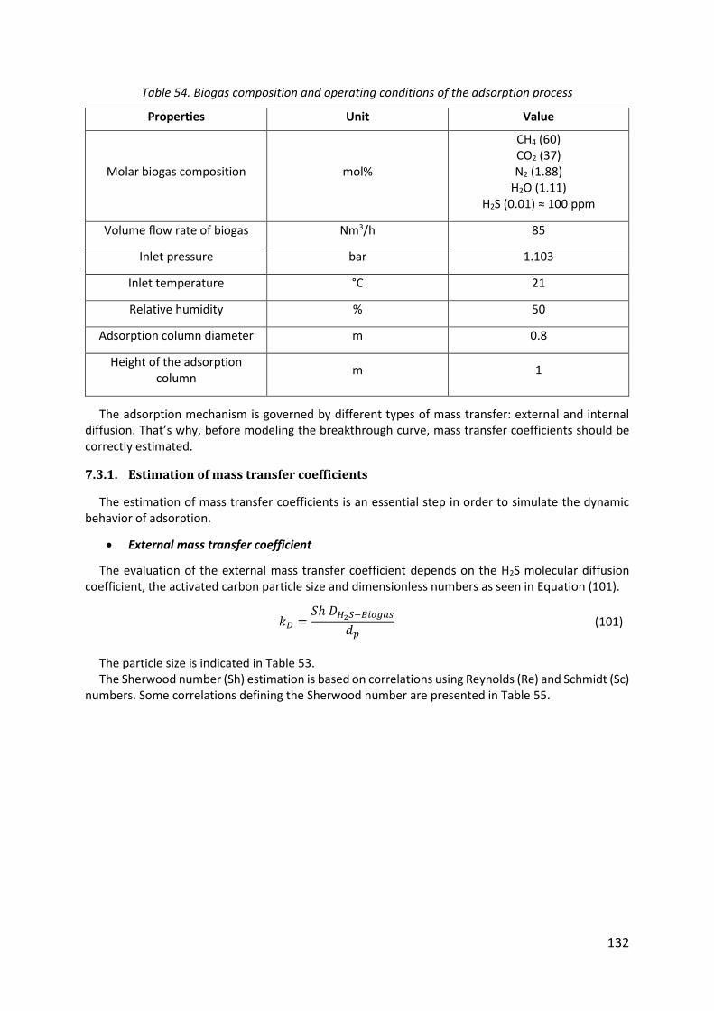
132
Table 54. Biogas composition and operating conditions of the adsorption process
Properties Unit Value
Molar biogas composition mol%
CH4 (60) CO2 (37) N2 (1.88)
H2O (1.11) H2S (0.01) ≈ 100 ppm
Volume flow rate of biogas Nm3/h 85
Inlet pressure bar 1.103
Inlet temperature °C 21
Relative humidity % 50
Adsorption column diameter m 0.8
Height of the adsorption column
m 1
The adsorption mechanism is governed by different types of mass transfer: external and internal diffusion. That’s why, before modeling the breakthrough curve, mass transfer coefficients should be correctly estimated.
7.3.1. Estimation of mass transfer coefficients
The estimation of mass transfer coefficients is an essential step in order to simulate the dynamic behavior of adsorption.
External mass transfer coefficient
The evaluation of the external mass transfer coefficient depends on the H2S molecular diffusion coefficient, the activated carbon particle size and dimensionless numbers as seen in Equation (101).
𝑘𝐷 =𝑆ℎ 𝐷𝐻2𝑆−𝐵𝑖𝑜𝑔𝑎𝑠
𝑑𝑝 (101)
The particle size is indicated in Table 53. The Sherwood number (Sh) estimation is based on correlations using Reynolds (Re) and Schmidt (Sc)
numbers. Some correlations defining the Sherwood number are presented in Table 55.
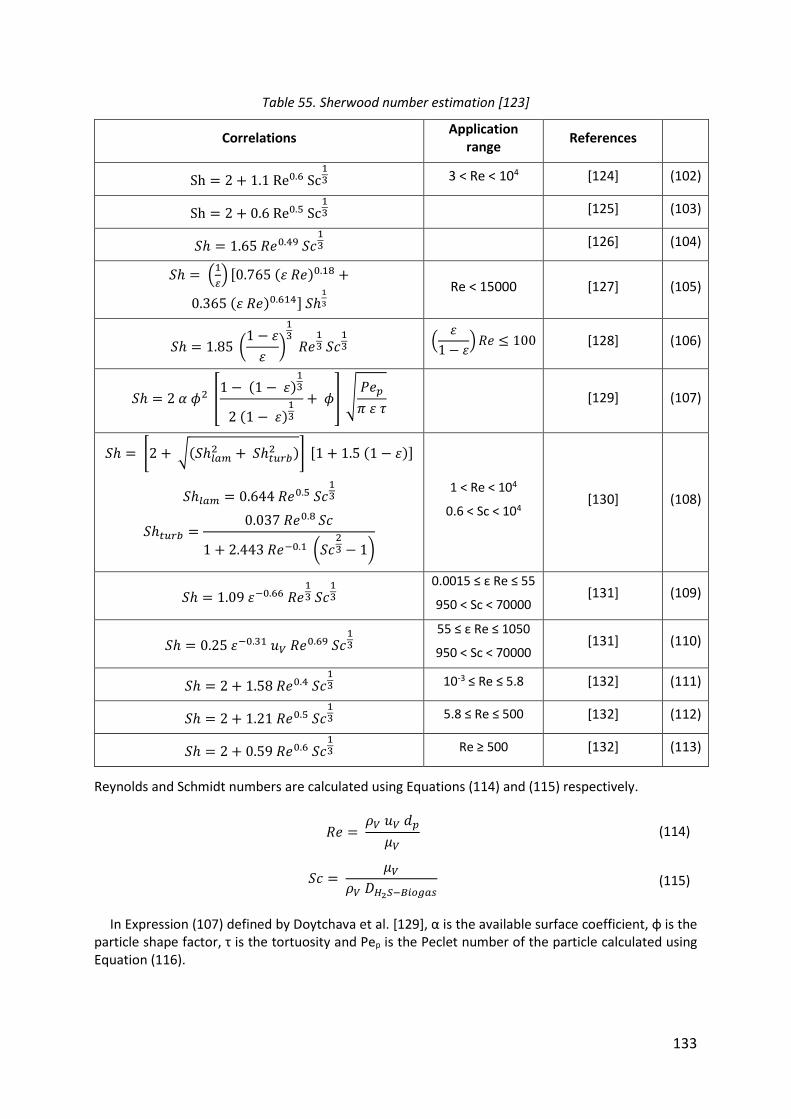
133
Table 55. Sherwood number estimation [123]
Correlations Application
range References
Sh = 2 + 1.1 Re0.6 Sc13 3 < Re < 104 [124] (102)
Sh = 2 + 0.6 Re0.5 Sc13 [125] (103)
𝑆ℎ = 1.65 𝑅𝑒0.49 𝑆𝑐13 [126] (104)
𝑆ℎ = (1
𝜀) [0.765 (휀 𝑅𝑒)0.18 +
0.365 (휀 𝑅𝑒)0.614] 𝑆ℎ1
3 Re < 15000 [127] (105)
𝑆ℎ = 1.85 (1 − 휀
휀)
13
𝑅𝑒13 𝑆𝑐
13 (
휀
1 − 휀) 𝑅𝑒 ≤ 100 [128] (106)
𝑆ℎ = 2 𝛼 𝜙2 [1 − (1 − 휀)
13
2 (1 − 휀)13
+ 𝜙] √𝑃𝑒𝑝
𝜋 휀 𝜏 [129] (107)
𝑆ℎ = [2 + √(𝑆ℎ𝑙𝑎𝑚2 + 𝑆ℎ𝑡𝑢𝑟𝑏
2 )] [1 + 1.5 (1 − 휀)]
𝑆ℎ𝑙𝑎𝑚 = 0.644 𝑅𝑒0.5 𝑆𝑐13
𝑆ℎ𝑡𝑢𝑟𝑏 =0.037 𝑅𝑒0.8 𝑆𝑐
1 + 2.443 𝑅𝑒−0.1 (𝑆𝑐23 − 1)
1 < Re < 104
0.6 < Sc < 104 [130] (108)
𝑆ℎ = 1.09 휀−0.66 𝑅𝑒13 𝑆𝑐
13
0.0015 ≤ ε Re ≤ 55
950 < Sc < 70000 [131] (109)
𝑆ℎ = 0.25 휀−0.31 𝑢𝑉 𝑅𝑒0.69 𝑆𝑐13
55 ≤ ε Re ≤ 1050
950 < Sc < 70000 [131] (110)
𝑆ℎ = 2 + 1.58 𝑅𝑒0.4 𝑆𝑐13 10-3 ≤ Re ≤ 5.8 [132] (111)
𝑆ℎ = 2 + 1.21 𝑅𝑒0.5 𝑆𝑐13 5.8 ≤ Re ≤ 500 [132] (112)
𝑆ℎ = 2 + 0.59 𝑅𝑒0.6 𝑆𝑐13 Re ≥ 500 [132] (113)
Reynolds and Schmidt numbers are calculated using Equations (114) and (115) respectively.
𝑅𝑒 = 𝜌𝑉 𝑢𝑉 𝑑𝑝
𝜇𝑉 (114)
𝑆𝑐 = 𝜇𝑉
𝜌𝑉 𝐷𝐻2𝑆−𝐵𝑖𝑜𝑔𝑎𝑠 (115)
In Expression (107) defined by Doytchava et al. [129], α is the available surface coefficient, φ is the particle shape factor, τ is the tortuosity and Pep is the Peclet number of the particle calculated using Equation (116).
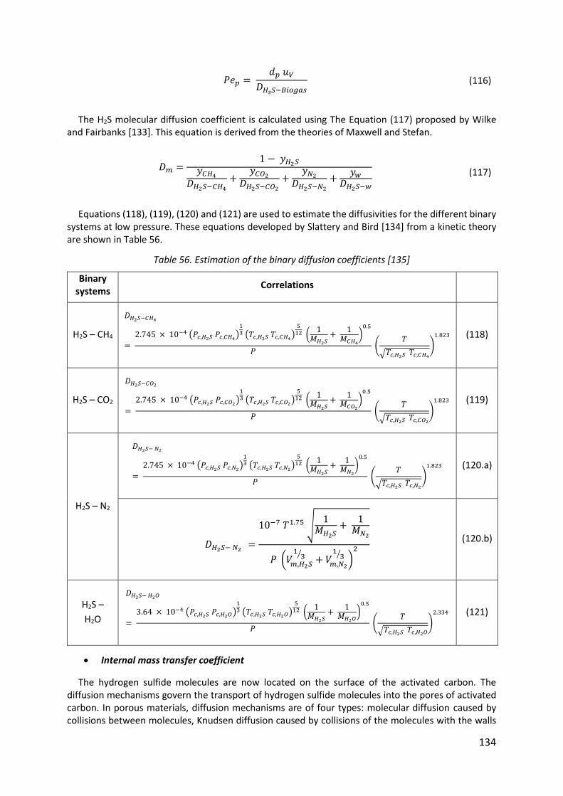
134
𝑃𝑒𝑝 = 𝑑𝑝 𝑢𝑉
𝐷𝐻𝑠𝑆−𝐵𝑖𝑜𝑔𝑎𝑠 (116)
The H2S molecular diffusion coefficient is calculated using The Equation (117) proposed by Wilke and Fairbanks [133]. This equation is derived from the theories of Maxwell and Stefan.
𝐷𝑚 =1 − 𝑦𝐻2𝑆
𝑦𝐶𝐻4
𝐷𝐻2𝑆−𝐶𝐻4
+𝑦𝐶𝑂2
𝐷𝐻2𝑆−𝐶𝑂2
+𝑦𝑁2
𝐷𝐻2𝑆−𝑁2
+𝑦𝑤
𝐷𝐻2𝑆−𝑤
(117)
Equations (118), (119), (120) and (121) are used to estimate the diffusivities for the different binary systems at low pressure. These equations developed by Slattery and Bird [134] from a kinetic theory are shown in Table 56.
Table 56. Estimation of the binary diffusion coefficients [135]
Binary systems
Correlations
H2S – CH4
𝐷𝐻2𝑆−𝐶𝐻4
=
2.745 × 10⁻⁴ (𝑃𝑐,𝐻2𝑆 𝑃𝑐,𝐶𝐻4)
13 (𝑇𝑐,𝐻2𝑆 𝑇𝑐,𝐶𝐻4
)5
12 (1
𝑀𝐻2𝑆+
1𝑀𝐶𝐻4
)0.5
𝑃 (
𝑇
√𝑇𝑐,𝐻2𝑆 𝑇𝑐,𝐶𝐻4
)
1.823
(118)
H2S – CO2
𝐷𝐻2𝑆−𝐶𝑂2
=
2.745 × 10⁻⁴ (𝑃𝑐,𝐻2𝑆 𝑃𝑐,𝐶𝑂2)
13 (𝑇𝑐,𝐻2𝑆 𝑇𝑐,𝐶𝑂2
)5
12 (1
𝑀𝐻2𝑆+
1𝑀𝐶𝑂2
)0.5
𝑃 (
𝑇
√𝑇𝑐,𝐻2𝑆 𝑇𝑐,𝐶𝑂2
)
1.823
(119)
H2S – N2
𝐷𝐻2𝑆− 𝑁2
=
2.745 × 10⁻⁴ (𝑃𝑐,𝐻2𝑆 𝑃𝑐,𝑁2)
13 (𝑇𝑐,𝐻2𝑆 𝑇𝑐,𝑁2
)5
12 (1
𝑀𝐻2𝑆+
1𝑀𝑁2
)0.5
𝑃 (
𝑇
√𝑇𝑐,𝐻2𝑆 𝑇𝑐,𝑁2
)
1.823
(120.a)
𝐷𝐻2𝑆− 𝑁2 =
10−7 𝑇1.75 √1
𝑀𝐻2𝑆+
1𝑀𝑁2
𝑃 (𝑉𝑚,𝐻2𝑆
13⁄
+ 𝑉𝑚,𝑁2
13⁄
)2
(120.b)
H2S –
H2O
𝐷𝐻2𝑆− 𝐻2𝑂
=
3.64 × 10⁻⁴ (𝑃𝑐,𝐻2𝑆 𝑃𝑐,𝐻2𝑂)13 (𝑇𝑐,𝐻2𝑆 𝑇𝑐,𝐻2𝑂)
512 (
1𝑀𝐻2𝑆
+ 1
𝑀𝐻2𝑂)
0.5
𝑃 (
𝑇
√𝑇𝑐,𝐻2𝑆 𝑇𝑐,𝐻2𝑂
)
2.334
(121)
Internal mass transfer coefficient
The hydrogen sulfide molecules are now located on the surface of the activated carbon. The diffusion mechanisms govern the transport of hydrogen sulfide molecules into the pores of activated carbon. In porous materials, diffusion mechanisms are of four types: molecular diffusion caused by collisions between molecules, Knudsen diffusion caused by collisions of the molecules with the walls
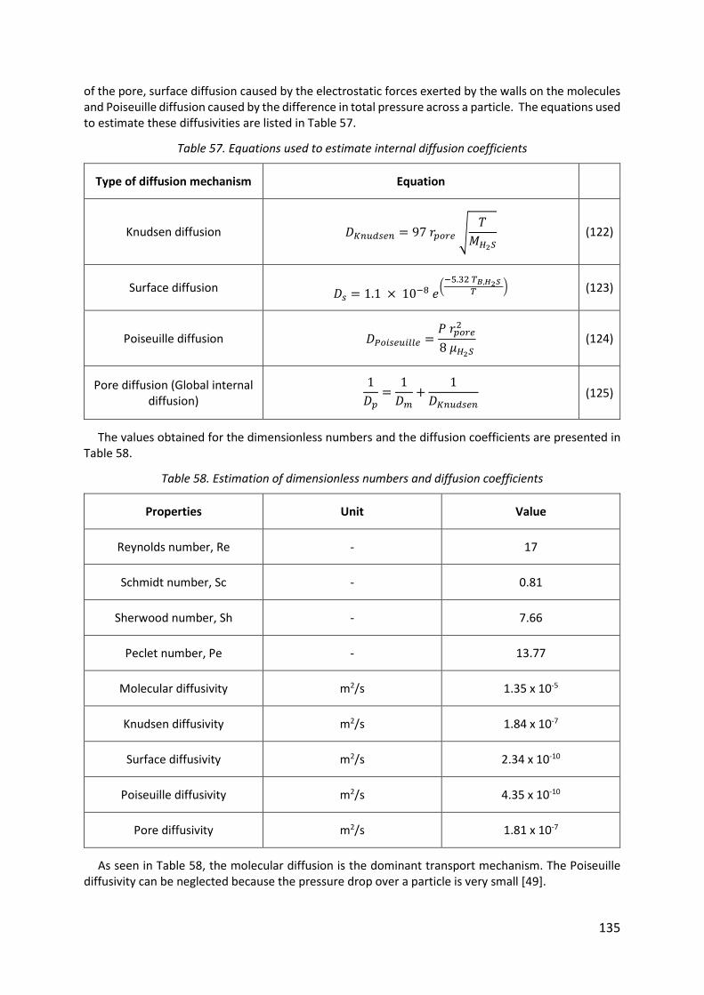
135
of the pore, surface diffusion caused by the electrostatic forces exerted by the walls on the molecules and Poiseuille diffusion caused by the difference in total pressure across a particle. The equations used to estimate these diffusivities are listed in Table 57.
Table 57. Equations used to estimate internal diffusion coefficients
Type of diffusion mechanism Equation
Knudsen diffusion 𝐷𝐾𝑛𝑢𝑑𝑠𝑒𝑛 = 97 𝑟𝑝𝑜𝑟𝑒 √𝑇
𝑀𝐻2𝑆 (122)
Surface diffusion 𝐷𝑠 = 1.1 × 10⁻⁸ 𝑒(
−5.32 𝑇𝐵,𝐻2𝑆
𝑇) (123)
Poiseuille diffusion 𝐷𝑃𝑜𝑖𝑠𝑒𝑢𝑖𝑙𝑙𝑒 =𝑃 𝑟𝑝𝑜𝑟𝑒
2
8 𝜇𝐻2𝑆 (124)
Pore diffusion (Global internal diffusion)
1
𝐷𝑝=
1
𝐷𝑚+
1
𝐷𝐾𝑛𝑢𝑑𝑠𝑒𝑛 (125)
The values obtained for the dimensionless numbers and the diffusion coefficients are presented in Table 58.
Table 58. Estimation of dimensionless numbers and diffusion coefficients
Properties Unit Value
Reynolds number, Re - 17
Schmidt number, Sc - 0.81
Sherwood number, Sh - 7.66
Peclet number, Pe - 13.77
Molecular diffusivity m2/s 1.35 x 10⁻⁵
Knudsen diffusivity m2/s 1.84 x 10⁻⁷
Surface diffusivity m2/s 2.34 x 10⁻¹⁰
Poiseuille diffusivity m2/s 4.35 x 10⁻¹⁰
Pore diffusivity m2/s 1.81 x 10⁻⁷
As seen in Table 58, the molecular diffusion is the dominant transport mechanism. The Poiseuille diffusivity can be neglected because the pressure drop over a particle is very small [49].
136
Knudsen diffusion and surface diffusion contribute to global internal diffusion. This contribution is very small compared to the contribution of external diffusion. Therefore, only external diffusion will be considered. The external mass transfer coefficient calculated using Equation (101) is equal to 0.021 m.s-1.
7.3.2. Modeling of breakthrough curves
The breakthrough curve is used to describe the spatiotemporal evolution of the concentration of H2S in the gas phase. This type of modeling the dynamics of the adsorption column is based on the definition of mass transfer balances: a mass balance of the gas phase where the transfer by convection dominates and a mass balance of the adsorbent particles where the diffusion transfer dominates [122].
Several hypotheses govern the flow of the biogas in the absorption column: The properties and the superficial velocity of the biogas are assumed constant throughout the adsorption column and the porosity of the adsorption column is considered uniform [136]. Based on the assumptions outlined, the mass balance of the adsorption column can be equated as seen in Equation (126). This equation has been used by several authors as Ruthven [49], Suzuki [137], Hwang et al. [138], Brosillon et al. [139], Yang [140], Boulinguiez [136] and Sigot [122].
−𝐷𝐿
𝐿2 𝜕2𝐶
𝜕𝑧2+
𝑢
𝐿 𝜕𝐶
𝜕𝑧+
𝜕𝐶
𝜕𝑡+
𝜌
휀 𝜕𝑞
𝜕𝑡= 0 (126)
Where:
DL [m2.s-1] is the axial dispersion coefficient. C [mol.m-3] is the concentration of H2S in the biogas. L [m] is the length of the adsorption column. z [m] is the axial dimension. t [s] is the time. u [m.s-1] is the superficial velocity of the biogas. ρ [kg.m-3] is the density of activated carbon. ɛ [-] is the void fraction of the adsorption column. q [g.kg-1] is the amount of H2S adsorbed per kg of activated carbon.
The mass balance Equation (126) takes into account the axial dispersion, convection, the accumulation of the gas phase and the overall mass transfer by adsorption [136]. To simplify the problem, initially the axial diffusion coefficient is neglected. The mass balance presented by Equation (126) is simplified.
𝑢
𝐿 𝜕𝐶
𝜕𝑧+
𝜕𝐶
𝜕𝑡+
𝜌
휀 𝜕𝑞
𝜕𝑡= 0 (127)
Considering a single transfer resistance material represented by the linear driving force model, the flux transferred may then be expressed relative to the solid phase concentration as shown in Equation (128), or relative to the gas phase concentration as shown in Equation (129).
𝜕𝑞
𝜕𝑡= 𝑘𝑔 𝑎𝑝 (𝑞𝑒 − 𝑞) (128)
𝜕𝑞
𝜕𝑡= 𝑘𝑔 𝑎𝑝
1 − 휀
𝜌 (𝐶 − 𝐶𝑒) (129)
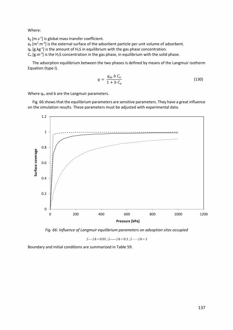
137
Where:
kg [m.s-1] is global mass transfer coefficient. ap [m2.m-3] is the external surface of the adsorbent particle per unit volume of adsorbent. qe [g.kg-1] is the amount of H2S in equilibrium with the gas phase concentration. Ce [g.m-3] is the H2S concentration in the gas phase, in equilibrium with the solid phase.
The adsorption equilibrium between the two phases is defined by means of the Langmuir isotherm Equation (type I).
𝑞 = 𝑞𝑚 𝑏 𝐶𝑒
1 + 𝑏 𝐶𝑒 (130)
Where qm and b are the Langmuir parameters.
Fig. 66 shows that the equilibrium parameters are sensitive parameters. They have a great influence on the simulation results. These parameters must be adjusted with experimental data.
Fig. 66: Influence of Langmuir equilibrium parameters on adsoption sites occupied
(……) b = 0.01 ; (____) b = 0.1 ; (- - - -) b = 1
Boundary and initial conditions are summarized in Table 59.
0
0.2
0.4
0.6
0.8
1
1.2
0 200 400 600 800 1000 1200
Surf
ace
co
vera
ge
Pressure [kPa]
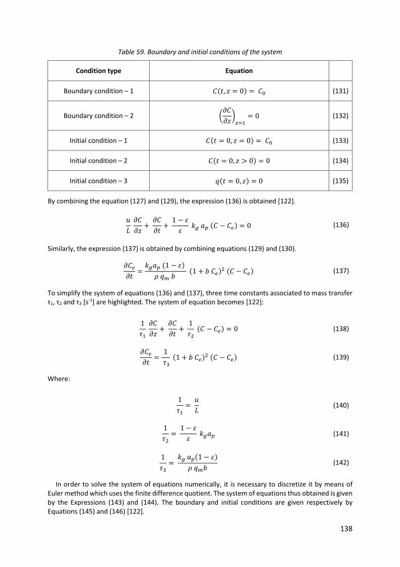
138
Table 59. Boundary and initial conditions of the system
Condition type Equation
Boundary condition – 1 𝐶(𝑡, 𝑧 = 0) = 𝐶0 (131)
Boundary condition – 2 (𝜕𝐶
𝜕𝑧)
𝑧=1= 0 (132)
Initial condition – 1 𝐶(𝑡 = 0, 𝑧 = 0) = 𝐶0 (133)
Initial condition – 2 𝐶(𝑡 = 0, 𝑧 > 0) = 0 (134)
Initial condition – 3 𝑞(𝑡 = 0, 𝑧) = 0 (135)
By combining the equation (127) and (129), the expression (136) is obtained [122].
𝑢
𝐿 𝜕𝐶
𝜕𝑧+
𝜕𝐶
𝜕𝑡+
1 − 휀
휀 𝑘𝑔 𝑎𝑝 (𝐶 − 𝐶𝑒) = 0 (136)
Similarly, the expression (137) is obtained by combining equations (129) and (130).
𝜕𝐶𝑒
𝜕𝑡=
𝑘𝑔𝑎𝑝 (1 − 휀)
𝜌 𝑞𝑚 𝑏 (1 + 𝑏 𝐶𝑒)2 (𝐶 − 𝐶𝑒) (137)
To simplify the system of equations (136) and (137), three time constants associated to mass transfer τ1, τ2 and τ3 [s-1] are highlighted. The system of equation becomes [122]:
1
𝜏1 𝜕𝐶
𝜕𝑧+
𝜕𝐶
𝜕𝑡+
1
𝜏2 (𝐶 − 𝐶𝑒) = 0 (138)
𝜕𝐶𝑒
𝜕𝑡=
1
𝜏3 (1 + 𝑏 𝐶𝑒)2 (𝐶 − 𝐶𝑒) (139)
Where:
1
𝜏1=
𝑢
𝐿 (140)
1
𝜏2=
1 − 휀
휀 𝑘𝑔𝑎𝑝 (141)
1
𝜏3=
𝑘𝑔 𝑎𝑝(1 − 휀)
𝜌 𝑞𝑚𝑏 (142)
In order to solve the system of equations numerically, it is necessary to discretize it by means of Euler method which uses the finite difference quotient. The system of equations thus obtained is given by the Expressions (143) and (144). The boundary and initial conditions are given respectively by Equations (145) and (146) [122].
139
𝐶𝑖𝑗+1
= −∆𝑡 [1
𝜏1 (
𝐶𝑖𝑗
− 𝐶𝑖−1𝑗
∆𝑧) +
1
𝜏2(𝐶𝑖
𝑗− 𝐶𝑒,𝑖
𝑗)] + 𝐶𝑖
𝑗 (143)
𝐶𝑒,𝑖𝑗+1
=∆𝑡
𝜏3 (1 + 𝑏 𝐶𝑒,𝑖
𝑗)
2(𝐶𝑖
𝑗− 𝐶𝑒,𝑖
𝑗) + 𝐶𝑒,𝑖
𝑗 (144)
𝐶1𝑗
= 𝐶0 𝑎𝑛𝑑 𝐶𝑛𝑗
= 𝐶𝑛−1𝑗
(145)
𝐶11 = 𝐶0 ; 𝐶𝑖>1
1 = 0 𝑎𝑛𝑑 𝐶𝑒,𝑖1 = 0 (146)
After the construction of the discrete form of the analytical mass balance equations, the input parameters for the simulation of the breakthrough curve are listed in Table 60.
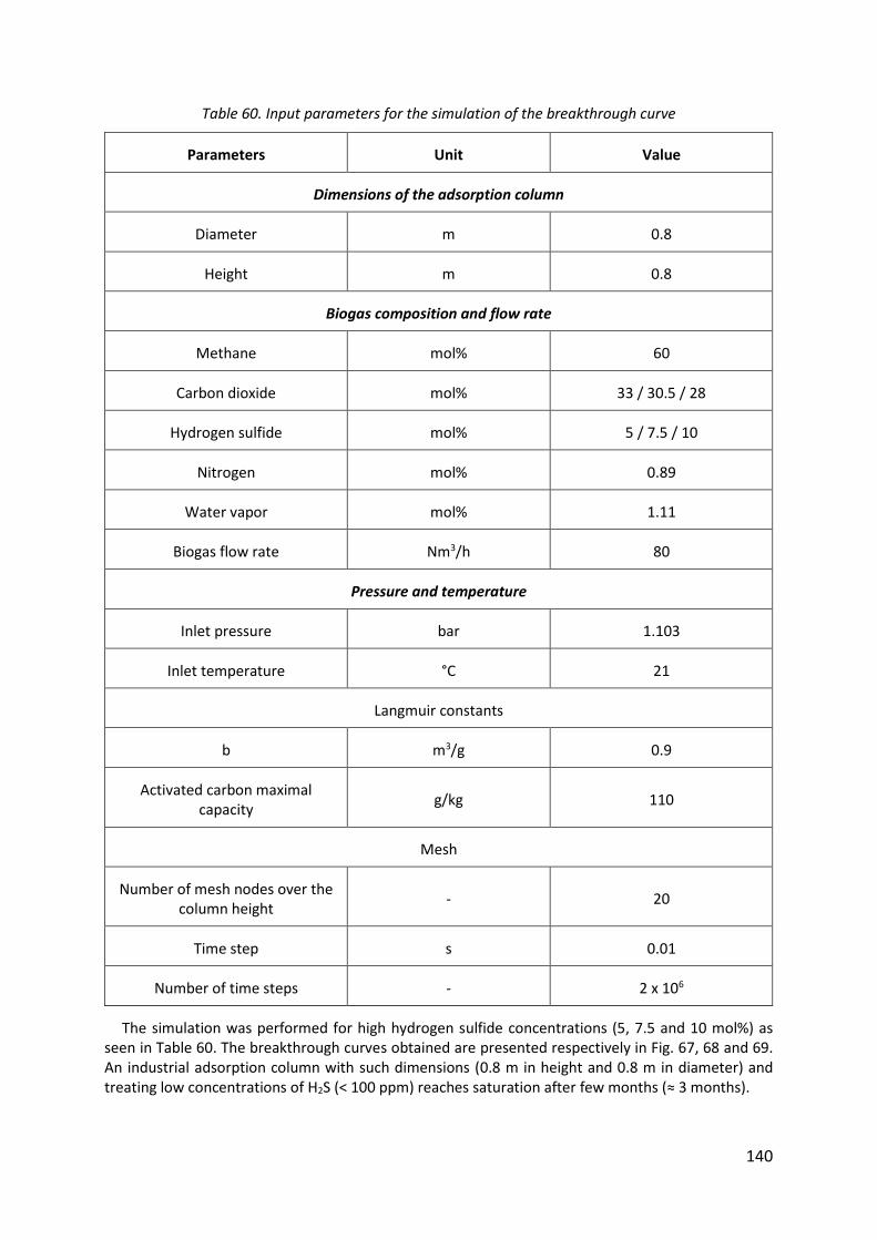
140
Table 60. Input parameters for the simulation of the breakthrough curve
Parameters Unit Value
Dimensions of the adsorption column
Diameter m 0.8
Height m 0.8
Biogas composition and flow rate
Methane mol% 60
Carbon dioxide mol% 33 / 30.5 / 28
Hydrogen sulfide mol% 5 / 7.5 / 10
Nitrogen mol% 0.89
Water vapor mol% 1.11
Biogas flow rate Nm3/h 80
Pressure and temperature
Inlet pressure bar 1.103
Inlet temperature °C 21
Langmuir constants
b m3/g 0.9
Activated carbon maximal capacity
g/kg 110
Mesh
Number of mesh nodes over the column height
- 20
Time step s 0.01
Number of time steps - 2 x 10⁶
The simulation was performed for high hydrogen sulfide concentrations (5, 7.5 and 10 mol%) as seen in Table 60. The breakthrough curves obtained are presented respectively in Fig. 67, 68 and 69. An industrial adsorption column with such dimensions (0.8 m in height and 0.8 m in diameter) and treating low concentrations of H2S (< 100 ppm) reaches saturation after few months (≈ 3 months).
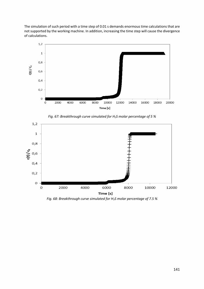
141
The simulation of such period with a time step of 0.01 s demands enormous time calculations that are not supported by the working machine. In addition, increasing the time step will cause the divergence of calculations.
Fig. 67: Breakthrough curve simulated for H2S molar percentage of 5 %
Fig. 68: Breakthrough curve simulated for H2S molar percentage of 7.5 %

142
Fig. 69: Breakthrough curve simulated for H2S molar percentage of 10 %
7.4. Conclusion
Based on the mass balance equations, a dynamic model has been developed to simulate the breakthrough curve for the system H2S – Activated carbon. To simulate the dynamic behavior of an adsorption column for the removal of low concentrations of H2S, a powerful calculation tool is necessary.
The results obtained with the model developed should be compared to experimental data in order to adjust the overall mass transfer coefficient and equilibrium parameters given by the Langmuir isotherm. The axial dispersion coefficient should be added in the mass balance equation to evaluate its contribution on the overall mass transfer coefficient.
This study has highlighted the analytical difficulties due to low concentrations of H2S. It has also showed the importance of the experimental work to develop an accurate model which could be a reliable design tool for biogas purification units.
143
Conclusions and perspectives
This thesis is part of the innovative project led by the Cryo Pur® society that aims to develop a technology to purify and upgrade biogas in order to be used as a liquid fuel or injected into the natural gas grid. The purpose of this work is to ensure a continuous removal of hydrogen sulfide upstream of the process because of the risks of toxicity, corrosion and odors.
This thesis has allowed drawing scientific and technical conclusions.
From a technical point of view, two desulfurization technologies were tested: chemical absorption in a packing column using sodium hydroxide as an aqueous solvent and adsorption using impregnated activated carbon in a fixed bed. Both techniques have been experimented on a demonstrator “BioGNVAL” developed by Cryo Pur® Society which treats 85 Nm3/h of real biogas from the sewage treatment plant of Valenton. The general process is characterized by the following conditions:
The concentrations of methane and carbon dioxide are about ≈ 60 mol% of CH4 and ≈ 35 mol% of CO2.
The process operates at a pressure slightly higher than the atmospheric pressure to prevent the infiltration of oxygen.
The desulfurization of biogas must be complete to ensure a high quality of CO2 and biomethane.
The concentration of H2S in the biogas is low and generally varies between 10 and 100 ppm.
Both technologies have shown satisfactory separation efficiency greater than 99.5 %. The bibliographic study has allowed choosing an efficient absorption process that uses sodium hydroxide as a chemical solvent for the selective separation of hydrogen sulfide. This method is based on contacting the biogas to be treated with the aqueous NaOH in a structured packing column.
Despite the advantages of this process, it also has some drawbacks. For example, in the presence of CO2, the aqueous solution of sodium hydroxide cannot be regenerated because there is formation of sodium carbonate (Na2CO3) precipitate. Moreover, when the tanks of NaOH and NaOCl reach their lowest level, they must be filled by an operator who has to handle hazardous products. This operation is an obstacle to the commercialization of the process which must be automated without the repetitive intervention of an operator. Nevertheless for high H2S concentrations for processes which are continuously operated with personnel, this absorption process can be adopted.
To overcome these drawbacks for fully automated biogas purification equipment, the adsorption technology using impregnated activated carbon was tested. It has achieved similar separation efficiencies to the absorption technology without the use of hazardous products and without the need for an operator to ensure continuous operation of the process. Furthermore, the investment and operating costs of the adsorption process are lower than those of the absorption process.
From a scientific point of view, experimental data collected on the BioGNVAL pilot plant were used to develop a new hydrodynamic model which predicts accurately the key hydrodynamic parameters in a structured packing column: liquid holdup, pressure drop, effective interfacial area and the two transition points: loading and flooding points. It also allows the design and optimization of structured packing columns to operate at full capacity. This model was developed based on an existing model: Billet and Schultes. Some constants and exponents present in the correlations of this last model were developed following a sensitivity analysis and then optimized based on experimental data to finally implement a new model adapted to predict precisely the hydrodynamic parameters of a small scale structured packing column used for biogas or natural gas applications.
144
After the hydrodynamic study, simulations using the chemical process optimization software Aspen Plus® V8.0 have been performed in order to determine the efficiencies of separation for different operating conditions. The rate-based model approach has been used. To describe vapor-liquid equilibrium, a γ/ϕ approach has been considered: the Electrolyte Non-Random Two-Liquid (ENRTL) model has been adopted to represent non-idealities in the liquid phase, while the Redlich-Kwong equation of state has been used for the vapor phase.
In order to improve the simulation of absorption, Henry’s law constants of the main biogas components (CH4, CO2 and H2S) in water, the properties of pure components, equilibrium constants for the equilibrium reactions and the reaction rate constant for the kinetically controlled reaction between carbon dioxide and the hydroxide ion have been verified against experimental data. After the verification and modification of the thermodynamic model, the results of the simulations were compared to experimental data obtained on the demonstrator “BioGNVAL”. The comparison shows that the two results are in good agreement. In connection with this work, it would be interesting to study the perspective of incorporating the hydrodynamic model developed, in the database of Aspen Plus.
For adsorption technology, a dynamic model has been developed to simulate the breakthrough curve for the system H2S – Activated carbon. During this study, the different mass transfer coefficients involved in the process have been estimated under the same conditions in which the experiments on “BioGNVAL” pilot plant were held.
The results obtained with the model developed should be compared to experimental data in order to adjust the overall mass transfer coefficient and equilibrium parameters given by the adsorption isotherm. Another perspective is to consider the reaction phenomena due to the impregnation of the activated carbon in order to have a prediction tool able to manage the design of adsorption columns. It will be also interesting to reinsert the axial dispersion coefficient in the mass balance equation to evaluate its contribution.
145
References
[1] Statistical department of the Ministry of Energy, France, 2014.
[2] EurObserv’ER, 2014, Biogas barometer.
[3] Benkimoun, P. and Landrin, S., 2016, “Diesel: 42000 morts prématurées chaque année en France.”, Journal le monde.
[4] De la Farge, B., 1995, “Le biogaz, procédés de fermentation méthanique.”, Masson.
[5] Zdanevitch, I., Masselot, G., Collet, S. and Bour, O., November 2009, “Etude de la composition du biogaz de
méthanisation agricole et des émissions en sortie de moteur de valorisation.”, Rapport d’étude n° DRC-09-94520-13867A.
[6] Walsh, J.L., Ross, C.C., Smith, M.S. and Harper, S.R., 1989, “Utilization of Biogas.”, Georgia Tech Research Institute,
Atlanta, Georgia 30332, USA, Biomass 20, 277-290.
[7] Walsh, J.L., Ross, C.C., Smith, M.S., Harper, S.R. and Wilkins, W.A., February 1988, “Handbook on biogas utilization.”,
Georgia Tech Research Institute, Atlanta, Georgia 30332, USA, Published for U. S. Departement of Energy, 133p.
[8] Pettersson, A., Losciale, M. and Liljemark, S., 2007, “LCMG – Pilotprojekt för LMG som fordonsbränsle i Sverige.”,
Report SGC 177. Vattenfall Power Consultant. Svenskt Gastekniskt Center.
[9] www.cryopur.com (Cryo Pur® company), accessed 25/07/2016.
[10] Rasi, S., Veijanen, A., and Rintala, J., 2007, “Trace compounds of biogas from di_erent biogas production plants.”,
Energy, 32(8) :1375–1380.
[11] Görisch, U., 2008, “La production de biogaz.”, Ulmer, Paris.
[12] Deublein, D., 2008, “Biogas from waste and renewable resources : an introduction.”, Wiley-VCH, Weinheim, Germany.
[13] Suez, G., IFP, and ADEME, 2009, “Etude biogaz - etat des lieux et potentiel du biométhane carburant.”, Technical report,
Groupe de Travail Energie-Environnement de l’Association FranÃ˘gaise du Gaz Naturel pour Véhicules.
[14] Boulinguiez, B. and Le Cloirec, P., 2011, “Purification de biogaz – Elimination des COV et des siloxanes.”, Techniques
de l’ingénieur.
[15] Buswell, A.M. and Neave, S.L., 1930, “Laboratory studies of sludge digestion.”, Department of Registration and
Education.
[16] IPCC, Intergovernmental Panel on Climate Change, 2016.
[17] Leclerc, E., 2015, “STEP d’Aquapole : Présentation de la méthanisation et de l’injection au réseau.”.
[18] Biard, P.F., 2009, “Contribution au développement d’un procédé de lavage chimique compact. Traitement du sulfure
d’hydrogène par le chlore à l’échelle semi-industrielle et de COV odorants par oxydation avancée O3 / H2O2 à l’échelle
du laboratoire.”, Thesis, University of Rennes 1, France.
[19] National Institute of Standars and Technology, NIST, 2016.
[20] Bosak, S., 2000, “Science is …: A source book of fascinating facts, projects and activities.”.
[21] World Meteorological organization, 2016.
[22] Kidnay, A.J., 1999, “Vapor-Liquid Equilibria in the Nitrogen + Carbon Dioxide + Propane System from 240 to 330 K at
Pressures to 15 MPa.”, J.Chem.Eng.Data 44, 926-931.
[23] Yarym-Agaev, N.L., 1999, “Vapor-Liquid Equilibrium and Volumetric Properties of the Liquid Phase of the gamma-
Butyrolactone-Carbon Dioxide System at Increasing Pressures.”, Zh.Prikl.Khim. 72, 1085-1089.
[24] Miller, E.E., 1942, “The Joule-Thomson Effect in Carbon Dioxide.”, J.Am.Chem.Soc. 64, 400-411.
[25] Del Rio, F., 1984, “The vapour pressure of CO2 from 194 to 243 K.”, J.Chem.Thermodyn. 16, 469-474.
[26] Stull, D.R., 1947, “Vapor Pressure of Pure Substances. Organic and Inorganic Compounds.”, Ind. Eng. Chem., 39, 4, 517-
540.
[27] Giauque, W.F. and Egan, C.J., 1937, “Carbon Dioxide. The Heat Capacity and Vapor Pressure of the Solid. The Heat of
Sublimation. Thermodynamic and Spectroscopic Values of the Entropy.”, J. Chem. Phys., 5, 1, 45-54.
[28] Prydz, R. and Goodwin, R.D., 1972, “Experimental Melting and Vapor Pressures of Methane.” J. Chem. Thermodyn., 4,
1, 127-133.
[29] Riva, M., Campestrini, M., Toubassy, J., Clodic, D. and Stringari, P., 2014, “Solid – Liquid – Vapor Equilibrium Models
for Cryogenic Biogas Upgrading.”, Industrial & Engineering Chemistry Research.
[30] Langè, S., Campestrini, M. and Stringari, P., 2016, “Phase Behavior of System Methane + Hydrogen Sulfide.”, AIChE
Journal.
[31] Kunz, O. and Wagner, W., 2012, “The GERG – 2008 Wide-Range Equation of State for Natural Gases and Other
Mixtures: An Expansion of GERG – 2004, ti be submitted to J. Chem. Eng. Data.
[32] Shao, T.H., 1963, “Engineering Heat Transfer.”, D. Van Nostrand Company, Inc. London.
[33] Vardanjan, R., Laizans, A., Jakovics, A. and Gendelis, S., 2015, “Biogas specific heat capacity variations during
upgrading.”, Engineering for rural development, University of Latvia.
[34] Gélin, P. and Primet, M., 2002, “Complete oxidation of methane at low temperature over noble metal based catalysts: a
review. Applied Catalysis B: Environmental.”, 39 (1): p. 1 - 37.
[35] The Danish Technological Institute, Danemark, 2012.
[36] Kohl, A. and Nielsen, R., 1997, “Gas purification, fifth edition.”, 331-402.
[37] Mokhatab, S. and Poe, W. A., 2006, “Handbook of natural gas transmission and processing.”, p. 255.
[38] Burr, B. and Lyddon, L., 2008, “A comparison of physical solvents for acid gas removal.”, p. 1.
[39] Lide, D.R., 2004, “Handbook Chemistry and physics.”, CRC Press, Boca Raton, FL, 85 edition.
[40] Bucklin, R.W. and Schendel, R.L., 1984, “Comparison of Fluor Solvent and Selexol Processes.”, Energy Progress.
[41] Descamps, C., 2004, “Etude de la capture du CO2 par absorption physique dans les systèmes de production d’électricité
basés sur la gazéification du charbon intégrée à un cycle combiné.”, Thesis, Ecole des Mines de Paris, p. 26.
[42] Archane, A., 2009, “Etude de l’absorption des gaz acides dans des solvants mixtes.”, Ecole des Mines de Paris, p. 6.
146
[43] Lecomte, F., Broutin, P. and Lebas, E., 2010, “Le captage du CO2, des technologies pour réduire les émissions de gaz à
effet de serre.”, IFP publications, Chapter 3, p. 43.
[44] Bottoms, R.R., 1930, “Process for separating acidic gases.”, Patent US 1783901.
[45] Pani, F., Gaunand, A., Richon, D., Cadours, R. and Bouallou, C., 1997, “Absorption of H2S by Aqueous
Methyldiethanolamine Solution at 296 and 343 K.”, J. Chem. Eng. Data. 1997, 42, 865-870.
[46] Blauwhoff, P.M.M., Versteeg, G.F. and Van Swaaij, W.P.M., 1984, “A Study on the Reaction between CO2, and
Alkanolamines in Aqueous Solutions.”, Chem. Eng. Sci.. 39, 207.
[47] Neumann, D.W. and Lynn, S., 1984, “Oxidative absorption of H2S and O2 by iron chelate solutions.”, AIChE Journal,
Vol. 30, p. 62 – 69.
[48] Roquet, D., 2002, “Modélisation et étude expérimentale de l’absorption réactive multiconstituants.”, Université de Pau et
des pays de l’Adour.
[49] Ruthven D.M., 1984, “Principles of adsorption and adsorption processes.”, John Wiley & Sons, University of New
Brunswick, Fredericton, 1984. tel-00462034
[50] Yan R., Chin T., Ng Y.L., Duan H., Liang D.T. et Tay J.H., 2004, “Influence of Surface Properties on the Mechanism of
H2S Removal by Alkaline Activated Carbons.”, Environmental Science & Technology 38, n°1, p. 316-323.
[51] Bandosz, T.J., 1999, “On the adsorption/oxidation of hydrogen sulfide on activated carbons at ambient temperatures.”,
Journal of Colloid and Interface Science 246 (1), 1-20.
[52] Abatzoglou, N. and Boivin, S., December 2008, “A review of biogas purification processes.”, Biofuels, bioproducts and
biorefining, volume 3, pages 42-71.
[53] www.desotec.com (Desotec® company), accessed 07/04/2016.
[54] Yasyerli, S., Ar, I., Dogu, G. and Dogu, T., 2002, “Removal of hydrogen sulfide by clinoptilolite in a fixed bed adsorber.”,
Chemical Engineering and Processing, 41(9) :785–792.
[55] Cosoli, P., Ferrone, M., Pricl, S. and Fermeglia, M., 2008, “Hydrogen sulphide removal from biogas by zeolite adsorption
: Part i. GCMC molecular simulations.”, Chemical Engineering Journal, 145(1) :86–92.
[56] Johns, M.W., 1987, “The simulation of gold adsorption by carbon using a film diffusion model.”, Thesis, University of
the Witwatersrand, Johannesburg.
[57] UOP, 1990, “UOP Molecular Sieves.”, UOP Brochure F-I979J, 1/90.
[58] Bouchemal, F. and Achour, S., 2007, “Essais d’adsorption de la tyrosine sur charbon actif en poudre et en grain.”,
Laboratoire de recherche en hydraulique souterraine et de surface, Laryss Journal n° 6, 81-89.
[59] Evans, R., Marconi, U.M.B. and Tarazona, P., 1986, “Capillary condensation and adsorption in cylindrical and slit-like
pores.”, Journal of the Chemical Society, Faraday Transactions 2, 82(10) :1763–1787.
[60] Lesage, N., 2005, “Etude d’un procédé hybride Adsorption / Bioréacteur à membranes pour le traitement des effluents
industriels.”, Thesis, The National Institute of Applied Sciences of Toulouse.
[61] Brunauer, S., Deming, L., Deming, W. and Teller, E., 1940, J. Am. Chem. Soc., 62, 1723.
[62] Langmuir, I., 1916, “The constitution and fundamental properties of solids and liquids.”, J. Am. Chem. Soc. 38, 2221–
2295.
[63] Freundlich, H.M.F., 1906, “Uber die adsorption in losungen.”, Z. Phys. Chem. 57, 385–470.
[64] Temkin, M.I., 1941, “Adsorption equilibrium and the kinetics of processes on nonhomogeneous surfaces and in the
interaction between adsorbed molecules.”, Zh. Fiz. Chim. 15, 296–332.
[65] Elovich, S.Y. and Larinov, O.G., 1962, “Theory of adsorption from solutions of non electrolytes on solid (I) equation
adsorption from solutions and the analysis of its simplest form, (II) verification of the equation of adsorption isotherm
from solutions.”, Izv. Akad. Nauk. SSSR, Otd. Khim. Nauk 2, 209–216.
[66] Toth, J., 2000, “Calculation of the BET-compatible surface area from any type I isotherms measured above the critical
temperature.”, J. Colloid Interf. Sci. 225, 378–383.
[67] Hamdaoui, O. and Naffrechoux, E., 2007, “Modeling of adsorption isotherms of phenol and chlorophenols onto granular
activated carbon. Part I. Two-parameter models and equations allowing determination of thermodynamic parameters.”,
147, 381–394.
[68] Ayoub, S., 2010, “Simulation et optimisation de procédés d’adsorption modulée en pression – Formulation et résolution
à l’aide de l’optimisation dynamique hybride.”, Thesis, Institut national polytechnique de Lorraine, p. 8.
[69] Shivaji, S., 2002, “Pressure Swing Adsorption.”, Ind. Eng. Chem. Res., 41, 1389-1392.
[70] Soni, V., Abildskov, J., Jonsson, G. and Gani, R., 2009, “A general model for membranebased separation processes.”,
Computers and Chemical Engineering, 33, 644-659.
[71] Szymczyk, A. and Fievet P., 2007, “Les procédés de filtration membranaire appliqués au traitement des eaux dans :
Traitement et épuration des eaux industrielles polluées – Procédés membranaires, bioadsorption et oxydation chimique.”,
Presses universitaires de Franche-Comté, Chapter 2.
[72] Lakshminarayanaiah, N., 1984, “Equations of Membrane.”, Biophysics Elsevier Science & Technology Academic Press,
Original from the University of Michigan, New York.
[73] Bowen, W.R. and Gan, Q., 1991, “Properties of microfiltration membranes: Adsorption of bovine serum albumin at
polyvinylidene fluoride membranes.”, Journal of Colloid and Interface Science, 144, 254-262.
[74] Chen, X.Y., 2012, “Développement de nouvelles membranes à base de polyimide pour la séparation CO2 / CH4.”, Thesis,
Université Laval, Québec.
[75] Farrusseng, D., 2011, “Metal-Organic Frameworks – Applications from catalysis to gas storage.”.
[76] Boucif, N., 2012, “Modélisation et simulation de contacteurs membranaires pour les procédés d’absorption de gaz acides
par solvant chimique.”, Université de Lorraine, Chapter 2, p. 26.
[77] Ohya, H., Kudryavsev, V.V. and Semenova, S.I., 1997, “Polyimide membranes: applications, fabrications and
properties.”, Chapter 5, p. 180.
147
[78] Schweigkofler, M. and Niessner, R., 2001, “Removal of siloxanes in biogases.”, Institute of Hydrochemistry, Technical
University Munich, 83(3):183-96.
[79] Hagmann, M., Heimbrand, E. and Hentschel, P.P., 1999, “Determination of siloxanes in biogas from landfills and sewage
treatment plants.”, Proceedings of the 7th International Waste Management and Landfill Symposium: Proceedings
Sardinia, Cagliari, Italy.
[80] Benjaminsson, J., 2006, “Nya renings - och uppgraderingstekniker för biogas. Report SGC163.”, Svenskt Gastekniskt
Center.
[81] Pettersson, A., Losciale, M. and Liljemark, S., 2006, “LCNG-stuide – möjligheter med LNG i fordonsgasförsörjningen i
Sverige.”, Report SGC 167. Vattenfall Power Consultant. Svenskt Gastekniskt Center.
[82] Johansson N., 2008, “Production of liquid biogas, LBG, with cryogenic and conventional upgrading technology.
Description of systems and evaluations of energy balances.”, Master thesis, Chapter 4, p. 16.
[83] Hagen, M., Polman, E., Jensen, J. K., Myken, A., Jönsson, O. and Dahl, A., 2001, “Adding gas from biomass to the gas
grid. Swedish gas center.”, (SGC Report N° 118).
[84] Benjaminsson, J., Johansson, N. and Karlsvärd, J., 2010, “Les gaz d’enfouissement comme carburant de
véhicule.”, Swedish gas center (SGC Report N° 214).
[85] Harasimowicz, M., Orluk, P., Zakrzwska-Trznadel, G. and Chmielewski, A.G., 2007, “Application of polyimide
membranes for biogas purification and enrichment.”, p. 698 – 702.
[86] Deng, L. and Hägg, M., 2010, “Techno-economic evaluation of biogas upgrading process using CO2 facilitated transport
membrane.”, p. 638 – 646.
[87] Le Cloirec, P., 1998, “Les Composés Organiques Volatils (COVs) dans l’Environnement.”, Tech. & Doc., Lavoisier,
Paris, 737 p, ISBN 2-7430-0232-8.
[88] Bauer, F., Hulteberg, C., Persson, T. and Tamm, D., 2013, “Biogas upgrading – Review of commercial technologies.”,
Swedish gas center (SGC Report N° 270).
[89] Clodic, D., El Hitti, R., Younes, M., Bill, A. and Casier, F., 2005, “CO2 capture by anti-sublimation – Thermo-economic
process evaluation.”, Paper presented at the 4th Annual Conference on Carbon Capture & Sequestration, May 2-5, 2005,
Alexandria (VA), USA.
[90] EIGA Publication AHG IGC 1.1, 1999, “Carbon Dioxide Source Certification, Qualify Standards and Verification.”,
European Industrial Gases Association.
[91] Strigle, R. F. Jr., 1994, “Packed tower design and applications, Random and structured packings, second edition.”.
[92] Chan, H. and Fair, J. R., 1983, “Industrial and Engineering Chemistry Process Design and Development”, 23-814.
[93] Emil Friedrich Paquet, 2011, “Establishing a facility to measure the efficiency of structured packing under total reflux.”,
MSc, Stellenbosch: University of Stellenbosch.
[94] Schultes, M., 2010, “Research on mass transfer columns "Old hat or still relevant ?".”, Distillation Absorption, Eindhoven,
The Netherlands, 37-42.
[95] Billet, R. and Schultes, M., 1993, “A physical model for the prediction of liquid hold-up in two-phase counter-current
columns.”, Chemical Engineering & Technology, 16:370-375.
[96] Fair, J.R., Rocha, J.A. and Bravo, J.L., 2000, “A comprehensive model for the performance of columns containing
structured packings.”, Institution of Chemical Engineers Symposium Series 128, Birmingham, 1:A489-A507.
[97] Olujić, Ž., Behrens, M., Colli, L. and Paglianti, A., 2004, “Predicting the efficiency of corrugated sheet structured packings
with large specific surface area.”, Chemical and Biochemical Engineering Quarterly 18:89-96.
[98] Billet, R. and Schultes, M., 1999, “Prediction of mass transfer columns with dumped and arranged packings: Updated
summary of the calculation method of Billet and Schultes.”, Chemical Engineering Research and Design 77:498-504.
[99] Lamprecht, S.M., 2010, “Establishing a facility to measure packed column hydrodynamics.”, MSc, Stellenbosch:
University of Stellenbosch.
[100] Erasmus, A.B., 2004, “Mass transfer in structured packing.”, Thesis, Departement of Process Engineering at the
University of Stellenbosch.
[101] Gualito, J.J., Cerino, F.J., Cardenas, J.C. and Rocha, J.A., 1997, “Design method for distillation columns filled with
metallic, ceramic, or plastic structured packings.”, Industrial & Engineering Chemistry Research 36:1747-1757.
[102] Taylor, R., Krishna, R. and Kooijman, H., 2003, “Real-World Modeling of Distillation,”, Chem. Eng. Prog., 28-39.
[103] Chen, C.C., Tremblay, D. and Bhat, C., 2008, “A Rate-Based Process Modeling Study of CO2 Capture with Aqueous
Amine Solutions using aspenONE Process Engineering.”.
[104] Chen, C.C. and Song, Y., 2004, “Generalized electrolyte-NRTL model for mixed-solvent electrolyte systems.”.
[105] Gillespie, P.C. and Wilson, G.M., 1982, “Vapor-liquid and liquid-liquid equilibria: water – methane, water – carbon
dioxide, water – hydrogen sulfide, water – n-pentane, water – methane – n-pentane.”, Research report RR-48, Gas
Processors Association.
[106] Harvey, A.H., 1996, “Semiempirical correlation for Henry’s constants over large temperature ranges.”, AIChE J. 42,
1491.
[107] Aly, F.A. and Lee, L.L., 1981, “Fluid Phase Equil.”, 6, 169-179.
[108] Elliott, J.R. and Lira, C.T., 1999, “Introductory chemical engineering thermodynamics.”.
[109] Herrington, T.M., Pethybridge, A.D. and Roffey, M.G., 1986, “Densities of aqueous lithium, sodium, and potassium
hydroxides from 25 to 75 °C at 1 atm.”, J. Chem. Eng. Data 31, 31–34.
[110] Jones, G. and Dole, M., 1929, J. Amer. Chem. Soc., 51, 2950.
[111] Breslau, B.R. and Miller, I.F., 1970, J. Phys. Chem., 74, 1056.
[112] Palaty, Z., 1992, “Viscosity of diluted aqueous K2CO3 / KHCO3 solutions.”, Collect. Czech. Chem. Commun., 57,
1879.
[113] Vargaftik, N.B., 1972, “Dictionary of thermophysical properties of gases and liquids.”.
148
[114] Pac, J.S., Maksimova, I.N. and Glushenko, L.V., 1984, “Viscosity of alkali salt solutions and comparative calculation
method.”, J. Appl. Chem. USSR., 57, 846.
[115] Klochko, M.A. and Godneva, M.M., 1959, “Electrical conductivity and viscosity of aqueous solutions of NaOH and
KOH.”, Russ. J. Inorg. Chem., 4, 964-968.
[116] Gel'perin, N.I., Gurovich, B.M. and Dubinchik, K.K., 1969, “The relation between the surface tension of aqueous
solutions of inorganic substances and concentration and temperature.”, J. Appl. Chem. USSR, 42, 190-192.
[117] Horvath, A.L., 1985, “Handbook of Aqueous Electrolyte Solutions.”.
[118] Edwards, T.J., Maurer, G., Newman, J. and Prausnitz, J.M., 1978, “Vapor-liquid equilibria in multicomponent
aqueous solutions of volatile weak electrolytes.”, AIChE J. 24 1978. 966–976.
[119] Pinsent, B.R., Pearson, L. and Roughton, F.J.W., 1956, “The kinetics of combination of carbon dioxide with
hydroxide ions.”, Trans. Faraday Soc., 52, 1512-1520.
[120] Faurholt, C., 1925, J. chim. physique, 21, 490.
[121] Sanchez, C., Couvert, A., Laplanche, A. and Renner, C., 2007, “Hydrodynamic and mass transfer in a new concurrent
two-phase flow gas-liquid contactor.”, Chemical Engineering Journal, 131, (1-3) 49-58.
[122] Sigot, L., 2015, “Epuration fine des biogaz en vue d’une valorisation énergétique en pile à combustible de type SOFC
: Adsorption de l’octaméthylcyclotétrasloxane et du sulfure d’hydrogène.”, Thesis, INSA Lyon, France.
[123] Baup, S., 2014, “Elimination de pesticides sur lit de charbon actif en grain en présence de matière organique naturelle
: Elaboration d’un protocole couplant expériences et calculs numériques afin de simuler les équilibres et les cinétiques
compétitifs d’adsorption.”, Thesis, Université de Poitiers.
[124] Wakao, N. and Funazkri, T., 1978, “Effect of Fluid Dispersion Coefficients on Particleto-Fluid Mass Transfer
Coefficients in Packed Beds.”, Chemical Engineering Science, 33, 1375-1384.
[125] Ranz, W.E. and Marshall W.R., 1952, “Evaporation from Drops.”, Chem. Eng. Prog., 48(4), 173.
[126] Wilke, C.R. and Hougen, O.A., 1945, “Mass Transfer in the Flow of gases through Granular Solids extended to Low
Modified Reynolds Numbers.”, Trans. Am. Inst. Chem. Eng., 41, 445-451.
[127] Dwivedi, P.N. and Upadhyay, S.N., 1977, “Particle-Fluid Mass Transfer in Fixed and Fluidized Beds.”, Ind. Eng.
Chem., Process Des. Dev., 16(2), 157-168.
[128] Kataoka, T., Yoshida, H. and Ueyama, K., 1972, “Mass Transfer in Laminar Region between Liquid and Packing
Materials Surface in the Packed-Bed.”, Journal of Chemical Engineering of Japan, 5(2), 132-136.
[129] Doytchava, B., Nikolova, A. and Peev, G., 1996, “Mass Transfer from Solid Particles to Fluid in Granular Bed.”,
Chemical Engineering Communications, 147, 183-195.
[130] Gnielinski, V., 1978, “Gleichungen zur Berechnung des Wärme- und Stoffaustausches in durchströmten ruhenden
Kugelschüttungen bei mittleren und grossen Pecletzahlen.”, VT Verfahrenstechnik, 12(6), 363-366.
[131] Wilson, E.J. and Geankoplis, C.J., 1966, “Liquid Mass Transfer at Very Low Reynolds Numbers in Packed Beds.”,
Industrial and Engineering Chemistry Fundamentals, 5(1),9-12.
[132] Onashi, H., Sugawara, T., Kikuchi, K.I. and Konno, H., 1981, “Correlation of Liquid-Side Mass Transfer Coefficient
for Single Particle and Fixed-Beds.”, Journal of Chemical Engineering of Japan, 14(6), 433-438.
[133] Wilke, C.R. and Fairbanks, D.F., 1950, “Diffusion coefficients in multicomponent gas mixtures.”, Industrial and
Engineering Chemistry Fundamentals, 42(3), pp 471-475.
[134] Slattery, J.C. and Bird, R.B., 1958, “Calculation of the diffusion coefficient of dilute gases and of the self-diffusion
coefficient of dense gases.”, AIChE Journal, Vol. 4, p. 137-142.
[135] Bird, R.B., Stewart, W.E. and Lightfoot, E.N., 1924, “Transport phenomena, 2nd edition.”, Chemical Engineering
Department. University of Wisconsin – Madison.
[136] Boulinguiez, B., 2010, “Procédé d’adsorption et régénération électrothermique sur textile de carbone activé : Une
solution pour la problématique des COV dans des gaz à fort potentiel énergétique.”, Thesis, University of Rennes 1,
France.
[137] Suzuki, M., 1990, “Adsorption Engineering.”, Elsevier Science Pub Co.
[138] Hwang, K.S., Choi, D.K., Gong, S.Y. and Cho, S.Y., 1997, “Adsorption and thermal regeneration of methylene
chloride vapor on an activated carbon bed.”, Chemical Engineering Science, 52 (7) : 1111 – 1123.
[139] Brosillon, S., Manero, M.H. and Foussard, J.N., 2001, “Mass Transfer in VOC Adsorption on Zeolite: Experimental
and Theoretical Breakthrough Curves.”, Environmental Science & Technology 35, n°17, p. 3571-3575.
[140] Yang, R.T., 2003, “Adsorbents: Fundamentals and Applications.”, Wiley-Interscience, Hoboken, New Jersey.

149
Résumé Le biogaz doit être purifié pour devenir un combustible
renouvelable. De nombreux traitements actuels ne sont
pas satisfaisants car, pour des raisons de coûts les
procédés de séparation privilégiés aboutissent souvent au
rejet direct ou indirect du sulfure d’hydrogène (H2S) à
l’atmosphère. C’est le cas de la séparation à l’eau sous
pression.
Les objectifs de la thèse portent d’abord sur l’étude et la
modélisation des méthodes connues de séparation de
l’hydrogène sulfuré du méthane. Les concentrations
typiques varient de 200 à 5000 ppm et la séparation devra
réduire la teneur résiduelle en H2S à moins de 1 ppm.
Parallèlement seront étudiées les méthodes de traitement
de H2S.
Une fois la (ou les) méthode(s) de séparation
sélectionnée(s), des essais de validation seront effectués
sur un système traitant de l’ordre de 85 Nm3/h de méthane
où seront injectées des quantités de H2S variant entre 1 et
100 ppm.
Cette thèse requiert des modélisations réalistes sous
Aspen Plus® ou sous un code équivalent pour établir a
priori des efficacités de séparation selon différentes
conditions opératoires et en prenant en compte le
paramètre température. L’énergie dépensée pour la
séparation effective sera un des critères fort de la
comparaison, de même que l’économie de matière.
Une approche système est indispensable pour étudier la
rétroaction de la méthode de valorisation du H2S sur la ou
les méthodes séparatives. A priori c’est aussi l’outil Aspen
Plus® ou équivalent qui permettra cette approche système.
L’étude du procédé sera menée selon la double approche
modélisation et expérimentation, pour l’étude
expérimentale des méthodes séparatives, l’échelle du banc
sera semi-industrielle et le banc permettra d’étudier les
méthodes de séparation jusqu’à -90°C.
Mots Clés Biogaz, Hydrogène sulfuré, Absorption réactive,
Adsorption sur charbon actif, Aspen Plus®,
Hydrodynamiques, Basses températures, Pilote
BioGNVAL, Carburant pour véhicules …
Abstract Biogas must be purified for becoming a renewable fuel.
At now, the most part of the purification techniques are
not satisfactory because they imply hydrogen sulfide
(H2S) rejection to the atmosphere. One example of
these methods is the treatment with high pressure
water.
The first objective of the thesis is modeling the
conventional methods for separating H2S from methane.
Typical concentrations of H2S in methane vary from 200
to 5000 ppm. Separation methods must decrease the
concentration of H2S in methane to less than 1 ppm. At
the same time, methods for H2S treatment will be
studied.
Once the most appropriated separation methods will be
selected, some test will be carried out on a pilot plant
capable of treating 85 Nm3/h of methane, where
quantities of H2S ranging from 1 and 100 ppm will be
injected. These tests will allow validating the modeling
of the separation process.
The thesis work requires simulating the separation
process using the software Aspen Plus® or an
equivalent one. The effectiveness of different operative
conditions will be tested, varying also the parameter
temperature. The energy necessary for the separation
will be one of the most important criteria for the
comparison, as well as the mass consumption of the
different fluids involved in the process.
A system approach is fundamental for evaluating the
backward effect of the H2S valorization method on the
separation techniques. The process simulator (Aspen
Plus® or equivalent) will allow the system approach.
The study will involve modeling and experimental parts.
The experimental part will be carried out taking
advantage of a semi-industrial size test bench, allowing
studying the separation methods down to -90°C.
Keywords Biogas, Hydrogen sulfur, Reactive absorption,
Adsorption on activated carbon, Aspen Plus®,
Hydrodynamics, Low temperatures, BioGNVAL pilot
plant, Vehicle fuel …