Embed Size (px)
Citation preview

STUDY ON THE EFFECT OF TOOL NOSE WEAR ON SURFACE
ROUGHNESS AND DIMENSIONAL DEVIATION OF WORKPIECE IN
FINISH TURNING USING MACHINE VISION
By
HAMIDREZA SHAHABI HAGHIGHI
Thesis submitted in fulfillment of the requirements for the degree of
Doctor of Philosophy
August 2008

ii
ACKNOWLEDGMENT
Praise God who has helped me to carry out this study.
First of all, I would like to express my sincere thanks to my supervisor,
Associate Professor Dr. Mani Maran Ratnam, for his support and motivation
throughout this research work. His guidance and advice have inspired me to generate
fruitful approaches in achieving the objectives of this research. Without his effort, I
would not be able to proceed and bring this research to a completion. Also, special
thanks go to all the lecturers of School of Mechanical Engineering who in one way
or another gave their valuable advice throughout this journey.
Also, I would like to appreciate Industrial Engineering Faculty of Amirkabir
University of Technology especially to Associate Professor Dr. Moattar husseini and
Associate Professor Dr. Karimi who encouraged and supported me to finalize this
research work. Beside that, I would like to thank Associate Professor Dr. Nourpanah,
Professor Dr. Najafpour and Associate Professor Dr. Biglari who encouraged me to
continue my study.
My gratitude is extended to my beloved parents, brothers and sisters who
supported me all along without hesitation. Also, I dedicate my special appreciate to
my lovely wife and daughter who always have been patient and encouraged me in
last three years. I treasure dearly their encouragement and moral support throughout
these years.
Last but not the least, my sincere thanks to Professor Dr. Rahmah Noordin
and her husband Mr. Riazy due to their unlimited kindness to my family.

iii
TABELE OF CONTENTS Page
Acknowledgement
Table of Contents
List of Tables
List of Figures
List of Abbreviations
List of symbols
Abstrak
Abstract
CHAPTER 1 INTRODUCTION
1.1 Background
1.2 Important types of tool wear
1.3 Overview of the methods of TCM and surface roughness detection
1.4 Problem statement
1.4.1 Importance of effect of nose wear on the surface quality of
workpiece
1.4.2 Importance of developing a method to predict the tool wear
and surface quality of workpiece
1.5 Objectives
1.5.1 First objective: Study on the effect of nose wear on the surface
ii
iii
x
xiii
xxi
xxii
xxiv
xxvi
1
1
3
5
9
9
10
12
12
iv
quality of turned parts
1.5.2 Second objective: Prediction of the flank wear, surface
roughness and dimensional deviation of workpiece in turning
operation using a statistical model
1.6 Outline of thesis
CHAPTER 2 LITERATURE REVIEW
2.1 Introduction
2.2 Early studies on TCM methods
2.3 Tool condition monitoring using indirect methods
2.4 Tool wear and surface roughness monitoring using vision systems
2.5 Prediction methods for surface roughness of workpiece
2.6 Summary
CHAPTER 3 IN-CYCLE MONITORING OF TOOL WEAR IN
TURNING OPERATION IN THE PRESENCE OF TOOL
MISALIGNMENT
3.1 Outline of the chapter
3.2 Importance of tool wear detection
3.3 Main types of lighting system used to study the tool wear
3.4 System set-up
3.4.1 Machine vision configuration
3.4.2 Machining condition
3.5 Wear measurement algorithm
13
15
17
19
24
27
56
62
66
66
66
68
69
69
72
72

v
3.5.1 Stage 1: Image acquisition
3.5.2 Stage 2: Image enhancement
3.5.3 Stage 3: Morphological operation
3.5.4 Stage 4: Segmentation
3.5.5 Stage 5: Conforming the worn and unworn cutting tool
3.5.6 Stage 6: Tool wear evaluation using subtraction method
3.5.7 Stage 7 and Stage 8: Notch wear detection in cutting tools
using gradient approach
3.5.8 Stage 9: Polynomial fitting
3.5.9 Stage 10: Determination of notch wear location
3.6 Results and discussion
3.6.1 Verification of wear area using optical microscope
3.6.2 System error evaluation of machine vision
3.6.2.1 Effect of tool misalignment on the results
3.6.2.2 Effect of different mask size on the results using
Wiener and median filtering
3.6.2.3 Effect of rotating and digitizing the images on the
vision system accuracy
3.6.3 Effect of ambient lighting and ambient vibration
3.6.3.1 Effect of ambient lighting
3.6.3.2 Effect of ambient vibration
3.6.4 Measurement of nose wear area
3.6.5 Notch wear detection
3.6.5.1 Determination of the best polynomial degree
3.6.5.2 Application to real images
74
75
79
81
82
89
91
96
96
96
97
100
100
101
105
107
107
109
110
111
111
114

vi
3.7 Summary
CHAPTER 4 STUDY ON THE EFFECT OF TOOL NOSE WEAR ON
FLANK WEAR (VBC) AND SURFACE ROUGHNESS OF
TURNED PARTS USING MACHINE VISION
4.1 Outline of the chapter
4.2 Importance of tool nose wear
4.3 Study on the effect of nose wear on surface roughness of workpiece
using machine vision
4.4 Nose wear as an indicator of flank wear in zone C (VBC)
4.5 System set-up
4.5.1 Machine vision configuration
4.5.2 Machining condition
4.6 Description of measurement algorithm
4.6.1 Algorithm used to detect the cutting tool profile
4.6.1.1 Detection of nose wear area of the cutting tool
4.6.1.2 Focusing the cutting tool nose area
4.6.1.3 The differences in radial distances of profiles of two
images in the polar system
4.6.1.4 Determination of flank wear (VBC)
4.6.2 Algorithm of flank wear (VBC) detection via surface roughness
4.6.2.1 Detection the surface profile of workpiece
4.6.2.2 Detection of flank wear (VBC) via surface profile of
116
118
118
118
120
122
126
126
131
133
133
133
135
141
142
143
143
147

vii
workpiece
4.7 Results and discussion
4.7.1 Error in surface roughness measurement
4.7.1.1 System error verification of surface roughness
measurement
4.7.1.2 Effect of ambient lighting
4.7.1.3 Effect of vibration
4.7.2 Nose wear area and its effect on surface roughness
4.7.2.1 Nose wear area measurement in mm2
4.7.2.2 Effect of nose wear area on surface roughness
4.7.3 Study on the effect of grooves on surface roughness
4.7.4 Detection of nose wear via cutting tool profile and surface
roughness of workpiece
4.7.5 Flank wear evaluation using nose wear profile
4.8 Summary
CHAPTER 5 PREDICTION OF SURFACE ROUGHNESS (Ra),
DIMENTIONAL DEVIATION (Dd) OF WORKPIECE
AND FLANK WEAR (VBC) USING 2-D IMAGES OF
CUTTING TOOL
5.1 Overview
5.2 System set-up
5.2.1 Machine vision configuration
5.2.2 Machining condition
151
151
151
154
155
156
156
157
166
168
170
171
174
174
178
178
179

viii
5.3 Methodology for predicting the surface roughness and dimensional
deviation of workpiece using machine vision and DOE
5.3.1 Determination of experiment size using FDM
5.3.2 Capturing the images and applying the image processing
techniques
5.3.3 Cropping the cutting tool nose area
5.3.4 Simulation of surface profile of workpiece
5.3.5 Surface roughness measurement from workpiece image
5.3.6 Determination of the dimensional deviation (Dd) of workpiece
5.3.7 Modeling and predicting the surface roughness and the
dimensional deviation of workpiece using RSM
5.4 Results and discussion
5.4.1 Evaluation of deviation in Dd and Ra using the conventional
measurement method
5.4.2 Comparison of Ra determined using real and simulated images
of workpieces for fixed cutting speed
5.4.3 Comparison of Ra determined using real and simulated images
of workpieces where the cutting speed is not fixed
5.4.4 Modeling and prediction of the surface roughness of
workpiece using 2-D image of cutting tool and RSM
5.4.5 Comparison between results of approximation model and
actual results
5.4.6 Optimization of the output responses using RSM
5.5 Summary
179
181
185
186
186
190
190
192
192
193
195
199
204
223
228
229

ix
CHAPTER 6 CONCLUSION AND FUTURE STUDY
6.1 Conclusion
6.2 Limitations of the method proposed and the solutions suggested
6.3 Future study
REFERENCES
PUBLICATION LIST
223
233
236
237
239
246

x
List of Tables Page Table 3.1. Horizontal and vertical scaling factors of vision system. Table 3.2. Machining parameters. Table 3.3. Horizontal and vertical scale factors of microscope. Table 3.4. Comparison the results of wear area of cutting tool (mm2) between
vision method and microscope. Table 4.1. Distances between measurement points on image (pixels). Table 4.2. Horizontal and vertical scaling factors. Table 4.3. Machining parameters used to study the system error of surface
roughness detection method. Table 4.4. Machining parameters used to study the effect of nose wear on
surface roughness of workpiece. Table 4.5. Machining parameters that used to study the effect of nose wear on
flank wear of cutting tools. Table 4.6. Comparison between aR and qR obtained using stylus method in
two different measurements in the same zone of the workpiece. Table 4.7. Comparison between roughness determined using vision method
and stylus method. Table 4.8. Machining parameters used to study the effect of nose wear area
on the surface roughness of workpiece. Table 4.9. Comparison between average value of nose wear obtained using
images of cutting tools Ni(C) and average value nose wear obtained using images of workpieces Ni(W).
Table 4.10. Flank wear (VBC) width (mm) determined using nose wear and
surface roughness and comparison with toolmaker’s microscope. Table 5.1. Horizontal and vertical scaling factors. Table 5.2. The variables levels of the experiments designed. Table 5.3. Tolerances of different classes of cutting tools Table 5.4. Machining condition.
71 72 98 99 131 131 132 132 133 152 153 165 169 170 179 182 193 195
xi
Table 5.5. Evaluation of deviation in values of Dd (μm) using profile projector.
Table 5.6. Comparison between values of Ra obtained from real images and
simulated images of workpieces machined between 1 min to 175 min.
Table 5.7. Machining parameters. Table 5.8. Evaluation of difference in values of Ra obtained from real images
of surface profiles of workpieces in different cutting speeds. Table 5.9. Comparison between values of Ra(r) and Ra(s) in different cutting
speeds (cs). Table 5.10. Evaluation of difference in Dd obtained from real images of
surface profiles of workpieces in different cutting speeds. Table 5.11. Comparison between Dd(r) and Dd(s) in different cutting speeds
(cs). Table 5.12. The machining parameters designed using factorial design
method. Table 5.13. Comparison between average roughness and dimensional
deviation obtained from real images of workpieces and the corresponding values determined using 2-D images of cutting tools used.
Table 5.14. Comparison between average roughness and dimensional
deviation obtained from approximation model and the corresponding values determined using 2-D images of cutting tools used.
Table 5.15. Comparison between average roughness and dimensional
deviation obtained from approximation model and the corresponding values determined using real images of workpieces.
Table 5.16. Comparison of flank wear measured between results obtained
from approximation model, microscope and 2-D images of cutting tools.
Table 5.17. The random machining parameters designed using factorial
design method. Table 5.18. Comparison of average surface roughness between results
obtained from approximation model and results obtained from real images of workpieces.
195 197 199 200 200 201 202 205 207 215 216 221 223 226

xii
Table 5.19. Comparison of dimensional deviation between results obtained from approximation model and results obtained from real images of workpieces.
Table 5.20. Comparison of flank wear between results obtained from
approximation model and results obtained from 2-D images of cutting tools.
Table 5.21. The optimized machining variables.
227 227 229

xiii
List of Figures Page Figure 1.1. (a) Top view of crater wear and nose profile and (b) flank wear land and notch wear of cutting tool based on ISO 3685 (1993). Figure 2.1. Schematic diagram of experimental set up. Figure 2.2. (a) Captured image of cutting tool and (b) contour of crater wear
detected using proposed method. Figure 2.3. Detected 3-D profile of crater wear area. Figure 2.4. Schematic diagram of laser scatter method set up to determine the
surface roughness Figure 2.5. Effect of light intensity on the images captured using front
lighting. Figure 2.6. Recognize of the true edge from the false edge. Figure 2.7. Tool wear detected using: (a) Front-lighting, (b) back-lighting and
(c) structure-lighting. Figure 2.8. Image of tool wear land segmented. Figure 2.9. Schematic diagram used to determine the crater wear depth of
cutting. Figure 2.10. Window used to match the pattern. Figure 2.11. The effect of window size on the results. Figure 2.12. System set up of off-line surface texture instrument. Figure 2.13. Real image of cutting tool: (a) Before applying the algorithm and
(b) after applying the algorithm. Figure 2.14. Error of the flank wear measured using algorithm of this study. Figure. 2.15. Effect of light direction on captured images. Figure 2.16. System setup of scattering method. Figure 2.17. Comparison between surface profile of workpiece using stylus
3 29 29 31 32 33 34 36 36 38 38 39 39 40 40 42 42 43

xiv
method and scattering method. Figure 2.18. Flank wear area and mass center of flank wear. Figure. 2.19. TWI versus surface roughness of workpiece. Figure 2.20. Schematic system set up used to determine the 3-D profile of
tool wear. Figure 2.21. Comparison between texture of workpiece surfaces using new
cutting tools and dull cutting tools. Figure 2.22. Results of VBC obtained using (a)-(b) Proposed method and (c)-
(d) toolmaker’s microscope. Figure 2.23. Some images of cutting tool captured using SEM. Figure 2.24. System set up used to capture the image of tool wear. Figure 2.25. Effect of fringe pattern on the wear area of cutting tool. Figure 2.26. 3-D images of cutting tool using CAD to study the tool wear. Figure 2.27. Optical geometry used to determine the 3-D profile of cutting
tool. Figure 2.28. Experimental set up used to capture the image of cutting tool. Figure 2.29. 3-D images of breakage: (a) Real image added the fringes and
(b) 3-D image of cutting tool mapped using phase shifting method.
Figure 2.30. Comparison between results of three methods used (Al-Kindi
and Shirinzadeh. Figure 2.31. The comparison between results obtained using design of
experiment method in: (a) VBB and Ra and (b) VBB and temperature.
Figure 2.32. FAN III structure for surface roughness. Figure 2.33. Effect of cutting speed on surface roughness when duration of
machining is fixed. Figure 2.34. Effect of Depth of cut on surface Roughness. Figure 3.1. Images of cutting tool captured using: (a) Front lighting and (b)
back lighting. Figure 3.2. Schematic diagram of tool wear monitoring system.
44 45 46 47 48 49 51 51 52 53 54 54 55 57 58 59 59 69 70
xv
Figure 3.3. Actual set-up of off-line tool wear monitoring system. Figure 3.4. Actual set-up of in-cycle tool wear monitoring system. Figure 3.5. Flow chart of algorithm used for tool wear measurement. Figure 3.6. (a)Blurred image of cutting tool and (b) intensity profile across A-
A of blurred image of cutting tool. Figure 3.7. (a) Sharp image of cutting tool and (b) intensity profile across A-A
of sharp image of cutting tool. Figure 3.8. Intensity profile across tool: (a) Before filtering (original), (b)
after median filtering (non-optimum), (c) median filtering (optimum) and (d) Wiener filtering (optimum).
Figure 3.9. Subtracted images: (a) Before removing noise, (b) after removing
noise by median filtering and (c) after removing noise by Wiener filtering.
Figure 3.10. Removal of micro-dust using opening and closing operations: (a)
Cutting tool tip, (b) area A before opening, (c) area A after opening and (d) area A after opening and closing.
Figure 3.11. Result of subtraction of two images before applying the
conforming method. Figure 3.12. Binary images (a) Image 1 and (b) Image 2 (before using
conforming method). Figure 3.13. Binary images: (a) Image 1 and (b) Image 2 after rotation (region
to be cropped is shown in dotted line). Figure 3.14. Image 1 and Image 2 after conforming. Figure 3.15. Result of subtraction of Image 1 and Image 2 after applying
conforming method. Figure 3.16. (a) Unworn cutting tool tip, (b) worn cutting tool tip after 40
minutes of machining and (c) wear area obtained by subtraction. Figure 3.17. Image of side view of cutting tool: (a) Before machining and (b)
after machining shown the built-up edge. Figure 3.18. (a)Simulated image of cutting tool having notch defect, (b) plot
of gradient values along profile and polynomial fitting and (c) plot of difference d(x) against distance along X-axis.
Figure 3.19. Scanning method to determine gradient at tool edge.
70 71 73 75 75 78 79 81 83 85 86 88 89 89 90 93 95

xvi
Figure 3.20. Comparison the results of wear area of cutting tool using vision
method and microscope. Figure 3.21. (a)-(d) Images captured using vision method from 4 cutting tools
used and (a´)-(d´) images captured using microscope. Figure 3.22. The system error before and after applying the conforming
algorithm. Figure 3.23. System error of subtracting two images of one cutting tool using
different filter mask size. Figure 3.24. The maximum and minimum error of subtraction of 20 images
of one cutting tool using median filtering. Figure 3.25. The maximum and minimum error of subtraction of 20 images
of one cutting tool using Wiener filtering. Figure 3.26. Standard deviation of subtraction 20 images using Wiener and
median filtering. Figure 3.27. Omitting some high intensity pixels: a) Cutting tool image
captured, b) the intensity of outside pixels of dark area are more than T and c) image stored of area A in computer using Thresholding method.
Figure 3.28. Gray level interpolation based on the nearest neighbor concept. Figure 3.29. Effect of light intensity: (a)-(b) Original image and its intensity
profile (light intensity 16 lux), (c)-(d) original image and its intensity profile (light intensity 854 lux) and (e)-(f) original image and its intensity profile (light intensity 1321 lux).
Figure 3.30. Effect of vibration on results: (a) Two successive images
subtracted and (b) graph of error of ten successive images subtracted.
Figure 3.31. Wear area of cutting tools for various machining time and
cutting speed. Figure 3.32. Variation of d(x)max – d(x)min with polynomial degree for
unworn cutting tool: (a) n = 3, (b) n = 5, (c) n = 11 and (d) n = 25. Figure 3.33. Variation of d(x)max - d(x)min with polynomial fitting order n. Figure 3.34. Notch wear detected on cutting tool having simulated notch.
99 99 101 102 103 104 104 106 107 108 109 111 112 113 114

xvii
Figure 3.35. Worn cutting tool with notch wear at various machining times: (a) 10 minutes, (b) 20 minutes, (c) 30 minutes and (d) 40 minutes. (Cutting speed: 134 m/min, feed rate = 0.25 m/min, depth of cut = 0.25 mm).
Figure 3.36. Worn cutting tool with notch wear at various machining times:
(a) 10 minutes, (b) 20 minutes, (c) 30 minutes and (d) 40 minutes. (Cutting speed: 191 m/min, feed rate = 0.25 m/min, depth of cut = 0.25 mm).
Figure 3.37. (a) Worn tool with notch wear detected for cutting speed 134
m/min, (b) variation of d(x) with distance along X for image in (a), (c) worn tool with notch wear detected for cutting speed 191 m/min and (d) variation of d(x) with distance along X for image in (c).
Figure 4.1. (a)-(b) Images of surface profiles of workpieces and (c)-(d)
images of cutting tools used. Figure 4.2. Two dimensional schematic shape of a periodic surface roughness
of workpiece produced using a lathe machine. Figure 4.3. Schematic of turning operation using a cutting tool. Figure 4.4. Section A-A in Figure 4.3 (Negative rake angle). Figure 4.5. Enlarged region of interest in Figure 4.4. Figure 4.6. (a) Actual set up and (b) schematic diagram of in-cycle surface
roughness monitoring system. Figure 4.7. (a) Actual setup and (b) schematic diagram of measurement
system of cutting tool rotation. Figure 4.8. Images of Ronchi rulings: (a)-(b) 25 mm lens and (c)-(d) 50 mm
lens. Figure 4.9. Flow chart of algorithm used to detect the tool wear. Figure 4.10. (a) Unworn cutting tool tip, (b) worn cutting tool tip after 26
minutes of machining and (c) nose wear area after subtraction (white area).
Figure 4.11. Tool tip of cutting tool (a) before rotating the corner area and (b)
after rotating the corner area. Figure 4.12. Cropped image of nose area of cutting tool in Figure 4.11(b).
115 115 116 122 122 123 124 125 127 129 130 134 135 137 138
xviii
Figure 4.13. Scanning method to detect the cutting tool profile (image rotated).
Figure 4.14. Superimposed plots of cutting tool profile: (a) Cartesian and (b)
polar coordinate system. Figure 4.15. Detection of nose wear using the surface profile (a) No.1, (b)
No.2 and (c) No.3. Figure 4.16. Flow chart of algorithm used to detect the surface profile of
workpiece. Figure 4.17. Images of surface roughness profile: (a) Before Wiener filtering,
(b) after Wiener filtering and (c) region where surface profile is captured.
Figure 4.18. Contour of roughness profile. Figure 4.19. Superimposed of detected surface profile of workpice (a)
Cartesian and (b) polar coordinate system. Figure 4.20. Detecting the nose wear using the surface profile and cutting tool
(a) No.1, (b) No.2 and (c) No.3. Figure 4.21. Comparison between roughness determined using vision method
and stylus method.
Figure 4.22. Images of surface roughness profile in the presence of ambient vibration: (a) First image, (b) second image and (c) subtraction of images in (a) and (b).
Figure 4.23. Images of cutting tool wear area: (a) After 1 min, (b) after 25 min, (c) after 50 min (d) after 75 min, (e) after 100 min, (f) after 125 min, (g) after 175 min and (h) after 208 min.
Figure 4.24. Plot of cutting tool wear area vs. machining time. Figure 4.25. Images of workpiece profiles: (a) After 1 min, (b) after 50 min,
(c) after 100 min and (d) after 175 min machining duration. Figure 4.26. Roughness profiles of workpieces: (a) After 1 min, (b) after 50
min, (c) after 100 min, and (d) after 175 min machining duration. Figure 4.27. Effect of feed rate and time of machining on Ra. Figure 4.28. Comparison between cutting tool profiles and workpiece surface
profiles for one wavelength: (a) After 1 min, (b) after 50 min, (c) after 100 min, and (d) after 175 min.
Figure 4.29. Effect of feed rate and nose wear on Ra.
139 140 142 144 145 146 149 150 154 155 157 158 158 159 160 161 163

xix
Figure 4.30. Effect of feed rate and nose wear on Ra. Figure 4.31. Effect of cutting tool rotation and feed rate on roughness value. Figure 5.1. Flow chart of algorithm used in this study. Figure 5.2. 3-D graph of response surface method. Figure 5.3. Cropped image of nose area of cutting tool (a) Original image (b)
Inverted the black pixels and the white pixels of image. Figure 5.4 Two dimensional schematic shape of a workpiece produced using
a lathe machine. Figure 5.5. (a) Simulated image of surface profile of workpiece before
machining (b) after one time rotation of machine spindle (c) two times rotation of machine spindle (d) five times rotation of machine spindle using a worn cutting tool.
Figure 5.6. Schematic diagram of superimposed workpiece surface profile
simulated using f1 and f2. Figure 5.7. Schematic diagram of workpiece machined using three feeds: f1, f2
and f3. Figure 5.8. Comparison between real images of workpieces and simulated
images of workpieces. Figure 5.9. Effect of feed rate and cutting speed on Ra for real images. Figure 5.10. Effect of feed rate and cutting speed on Dd for real images. Figure 5.11. Comparison between real images of workpieces and simulated
images of workpieces. Figure 5.12. Comparison between Ra using real and simulated images. Figure 5.13. Comparison between Dd using real and simulated images. Figure 5.14. Comparison the Ra values between results using approximation
model and simulated images of workpieces. Figure 5.15. Comparison the Dd values between results using approximation
model and simulated images of workpieces. Figure 5.16 Image of flank wear land of cutting tool captured using a digital
camera.
166 167 180 183 186 188 189 191 194 198 203 204 206 208 208 217 217 219

xx
Figure 5.17. Comparison the VBC values between the results using 2-D image of cutting tool and the results obtained from toolmaker’s microscope.
Figure 5.18. Comparison the VBC values between the results using
approximation model and the results obtained from 2-D image of cutting tools.
Figure 5.19. Comparison between the binarized real images of cutting tools
used in: (a)-(e) This subsection (samples 11, 12, 15, 20, 28 respectively) and (f)-(j) those that were used in Subsection 5.4.4 (samples 11, 12, 15, 20, 28 respectively).
222 222 225

xxi
LIST OF ABBREVIATIONS
AE
CCD
2-D
3-D
AI
DOE
TCM
HSS
RMS
RSM
CMM
SEM
PC
LWDM
ITC
FAN
FBFN
LDA
ANFIS
BUE
ROI
TWI
Acoustic emission
Charged couple device
Two dimensional
Three dimensional
Artificial intelligence
Design of experiments
Tool condition monitoring
High speed steel
Root mean square
Response surface method
Coordinate measuring machine
Scanning electron microscope
Personal computer
Long working distance microscope
Intensity-topography compatible
Fuzzy adaptive network
Fuzzy basis function network
Linear discriminant analysis
Adaptive neuro-fuzzy inference system
Built-up edge
Region of interest
Tool wear index

xxii
LIST OF SYMBOLS
VBC
VBB
Ni(W)
Ni(C)
Dd
VBN
VBBmax
λ
α
Rwc
Ruc
Ra
Rq
s
Ra(r)
Ra(s).
Ra(a)
Dd(r)
Dd(s)
Dd(a)
flank wear land width in nose area of relief face of cutting tool
flank wear land width in zone B of relief face of cutting tool
effect of nose wear on the surface roughness of workpiece
nose wear of cutting tool
dimensional deviation of workpiece
notch wear width in relief face of cutting tool
Maximum flank wear land width
rake angle of cutting tool
relief angle of cutting tool
radial distance of profile of worn cutting tool to the center of nose radius
of cutting tool
radial distance of profile of unworn cutting tool to the center of nose
radius of cutting tool
the value of centerline average of surface roughness
the value of root mean square of surface roughness
standard deviation
roughness value measured using real images of workpiece
roughness value measured using simulated images of workpiece
roughness value measured using approximation model
dimensional deviation using real images of workpiece
dimensional deviation value measured using simulated images
dimensional deviation measured using approximation model

xxiii
VBC(m)
VBC(2D)
VBC(a)
flank wear width measured using microscope
flank wear width measured using cutting tool images
flank wear width measured using approximation model

xxiv
KAJIAN KE ATAS KESAN KEHAUSAN MUNCUNG ALAT PADA
KEKASARAN PERMUKAAN DALAM OPERASI PELARIKAN
MENYUDAH DENGAN MENGGUNAKAN PENGLIHATAN MESIN
ABSTRAK
Operasi pemesinan merupakan suatu kaedah umum bagi menghasilkan
komponen-komponen mekanikal yang dikeluarkan di segenap pelusuk dunia.
Permintaan terhadap perkakas mesin dalam setahun dilaporkan mencecah lebih
daripada £10 bilion. Walau bagaimanapun, kegagalan mata alat memotong
menyebabkan masa-henti proses pemotongan yang tidak dijangkakan lalu
mengurangkan produktiviti dan meningkatkan kos pengeluaran. Masa-henti yang
disebabkan kegagalan mata alat dianggarkan lebih kurang 20% daripada masa
pemesinan. Dijangkakan bahawa kaedah pemantauan keadaan mata alat (TCM) yang
tepat dan boleh dipercayai boleh meningkatkan produktiviti antara 10% hingga 40%.
TCM yang menggunakan kaedah dalam-proses dan dalam-kitaran mampu menilai
kestabilan proses pemesinan, meningkatkan produktiviti, mengurangkan kesan tidak
dijangkakan yang boleh merosakkan perkakas mesin, serta meningkatkan kualiti
permukaan pada bahagian yang dimesin. Kajian tentang kualiti permukaan dan
kejituan dimensi hasil kerja adalah penting kerana kedua-dua parameter ini memberi
kesan terhadap prestasi komponen yang dimesin. Walau bagaimanapun, kajian
terdahulu, yang dilaporkan dalam literatur, tidak mampu mengenal pasti semua jenis
kehausan mata alat yang utama, yang memberi kesan terhadap kekasaran permukaan
hasil kerja. Walaupun diketahui bahawa profil mata alat pemotong memberi kesan
terhadap kekemasan produk, kesan kehausan muncung pada kekasaran permukaan

xxv
belum diselidik dalam kajian terdahulu. Kebanyakan kajian memberi tumpuan
terhadap kesan kehausan-rusuk pada kekasaran permukaan hasil kerja dengan
menggunakan kaedah tidak langsung. Penyelidikan ini bertujuan mengkaji kesan
langsung kehausan-muncung mata alat terhadap kekasaran permukaan dengan
menggunakan imej 2-D pada hujung mata alat dalam operasi pemutaran-kemasan.
Reka bentuk faktoran dan kaedah permukaan respons (RSM) digunakan untuk
meramal kekasaran permukaan dan sisihan dimensi hasil kerja dalam pelbagai
keadaan pemesinan Teknik reka bentuk eksperimen (DOE) berstatistik digunakan
untuk mengurangkan saiz eksperimen tanpa memberi kesan terhadap kejituan hasil.
Data yang digunakan dalam kajian ini dijana menggunakan kaedah simulasi imej 2-
D pada kawasan pemotongan–muncung yang digunakan untuk menghasilkan profil
permukaan hasil kerja. Ciri-ciri permukaan dalam imej yang dirangsang disari untuk
menentukan kekasaran purata (Ra) dan sisihan dimensi (Dd) hasil kerja. Lebar
bahagian kehausan-rusuk dalam kawasan muncung (VBc) juga dapat ditentukan
daripada kehausan-muncung dan kekasaran permukaan hasil kerja. Kejituan kaedah
yang dicadangkan dibandingkan dengan kaedah konvensional dengan menggunakan
penguji kekasaran permukaan dan mikroskop pembuat perkakas.

xxvi
STUDY ON THE EFFECT OF TOOL NOSE WEAR ON SURFACE
ROUGHNESS AND DIMENSIONAL DEVIATION OF WORKPIECE IN
FINISH TURNING USING MACHINE VISION
ABSTRACT
The aim of this research is to study the direct effect of tool nose wear which
is in contact to the surface profile of workpiece directly, on the surface roughness
and dimensional deviation of workpiece using a developed machine vision in finish
turning operation. The data used in this study were generated using a simulation
method whereby 2-D images of cutting tool nose area were used to simulate the
surface profile of the workpiece. The surface features in the simulated images were
extracted to determine the average roughness (Ra) and dimensional deviation (Dd) of
the workpiece. The flank wear in the nose area (VBC) was also determined from the
2-D image of cutting tool and the surface roughness of the workpiece. The response
surface method (RSM) was used to predict the surface roughness and dimensional
deviation of workpiece under various machining conditions. The results showed that
R-squared statistical parameter obtained using RSM for Ra, Dd and VBC are 0.997,
0.989 and 0.99. The results of proposed method were compared with the
conventional methods using surface roughness tester and optical microscope. The
deviation between proposed method and microscope for tool wear measurement is
about 5.5% and the deviation between proposed method and surface roughness tester
was about 3.2%. Proposed method of using 2D image of cutting tool shaped by nose
wear could measure and predict Ra, Dd and VBC. The results showed that the
deviation between actual values and the values predicted for Ra, Dd and VBC are 9%,
11.4% and 12% respectively. The proposed method is easy to carry out in the

xxvii
workshop area, easy to maintain and easy to understand because assessing the
images of cutting tool is easy. Also, this method is flexible to use for different
machining process because capturing the 2-D images of most of the cutting tool
inserts is possible using this method.

1
Chapter 1
Introduction
1.1 Background
An important method of production is machining operation, which is used to
remove material from a workpiece using a cutting tool. Turning, milling and drilling
are some important machining processes that are used to shape products (Sortino
2003). It is well known that machining operations have a significant role in
manufacturing process. According to Child et. al. (2000) the demand for machine
tools from the producers of machine tools in one year was more than £10 billion.
The economic and technological importance of cutting process have
encouraged many researchers to study this field in order to increase productivity,
quality of products, stability and safety of the machining while decreasing the costs
of production. Tool failure, which is the major cause of unpredictable downtime of
cutting process, not only increases production time and cost but also decreases the
productivity (Rehorn et. al. 2005). The downtime due to tool failure alone is
estimated to be about 20% of machining process time (Kurada and Bradley 1997 b).
It has been suggested that a reliable and precise tool condition monitoring (TCM)
method can increase the cutting speed between 10% and 50%, thus increasing the
productivity between 10% and 40% (Castejon et. al. 2007, Rehorn et. al. 2005).

2
There are many scientific publications on TCM. Kurada and Bradley (1997 a)
reported on vision systems used to detect the wear area of cutting tool directly.
Dimla (2000) and Rehorn et. al. (2005) reviewed some studies on TCM that mostly
focused on indirect methods. Lanzetta (2001) classified the important types of tool
failure in order to make the tool condition monitoring easier.
Automation is a significant goal in advanced machining industries in order to
increase productivity and decrease product costs. However, tool wear is a significant
limitation to implement the idea of unmanned machining. Manufacturers can
decrease production cost and increase productivity if they are able to change worn
out cutting tools just in time. Meanwhile, the size of tool wear, which affects the
cutting tool, is very small and cannot efficiently be observed using the naked eyes.
Thus, a toolmaker’s microscope is conventionally used with a magnification more
than 30 times to measure the tool wear (Trent 1991). This requires the tool to be
removed from the machine, thus disrupting the machining process.
The time of cutting tool replacement is possible to evaluate using the
statistical methods (Kerr et. al. 2006) or using TCM methods. Meanwhile, the
complicated effects of known and unknown parameters on machine operations have
made the tool wear as a challenging scientific study (Tay et. al. 2002). There are lots
of scientific reports published that each one was aimed to solve only a part of tool
wear study. More than 1400 published work were reviewed by Dan and Mathew
(1990), Teti (1995), Byrne et. al.(1995), Sick (2002), Dimla (2000), Rehorn et. al.

3
(2005). Most of these works were focused on TCM especially on tool wear and its
effect on products machined.
1.2 Prediction the surface quality of workpiece
Study on surface quality and dimensional accuracy of workpiece is very
important because these two parameters affect the performance of the parts machined
(Risbood et. al. 2003). Also, the surface profile of workpiece is a suitable parameter
to distinguish a worn out cutting tool from an unworn cutting tool (Mannan et. al.
2000). Therefore, the studies reported by Benardos and Vosniakos (2003) were
carried out to predict the surface quality of workpiece.
Although, stylus method is reliable for measuring the surface roughness of
workpieces accurately, use of stylus is not possible when the vibration exists in the
environment. Also, the stylus and its transducer can be easily damaged if excessive
force is applied. Therefore, the stylus method is not suitable for use on-line or in-
cycle to measure the roughness value (Tay et. al. 2003). Also, this method is not fast
and the stylus tip can damage the surface texture of parts machined if the workpieces
are soft material e.g. aluminum and plastics (Whitehouse 1994). In contrary, vision
methods are able to evaluate different specifications of surface roughness fast and
accurate because capturing and assessing the images using vision systems are easy.
Also, machine vision does not damage the surface quality of workpieces because this
method is a non-contact method.
Benardos and Vosniakos (2003) classified the studies of predicting the
surface quality of parts machined into four main groups. These groups are based on:

4
• The machining theories (these methods are based on metal cutting
theories).
• The conventional analysis (these methods use the effect of various
machining factors on surface profile of workpiece).
• The artificial intelligence (AI) methods (two important methods are
fuzzy-set-based technique and neural network method).
• The design of experiments (DOE) (these methods are based on the
statistical methods).
Benardos and Vosniakos (2003) suggested the advantages and limitations of
methods mentioned above to predict the surface roughness and dimensional
deviation of workpiece as follows:
• The machining theories: Although the background of machining theory
methods is well established, these methods have not led to a
comprehensive solution yet, and the existing methods using the
machining theory have not accurately estimated the surface roughness.
• The conventional analysis: Analysis of machining parameters such as
cutting speed, feed, and depth of cut based on the level of understanding
of the machining condition is not difficult to carry out, but these methods
require doing many experiments.
• The AI methods: The experiments based on intelligent methods are used
widely because these methods are not sensitive to noisy data, and these
methods do not need to be formulated to solve the problem. However,

5
according to Benardos and Vosniakos (2003) these methods are not
implemented in real applications of predicting the surface roughness
because there is no guarantee for their performance.
• The DOE methods: The statistical background of design of experiment
methods is well established, and the outputs of these methods are reliable.
In a scientific study, the experiments must be planned effectively to
achieve the aim of the study. The size of experiments also has to be
reduced to save the time and the cost. DOE methods are capable to reduce
the size of experiments without decreasing the accuracy of predicting.
Thus, many researchers have used these methods widely.
1.3 Effect of nose wear on surface roughness of workpiece using machine
vision
It is well known that the nose area of cutting tool is one of the main
parameters shaping the surface profile of workpiece (ISO 3685, 1993). Thus, the
nose wear, which is formed on the nose area of cutting tool, has an important effect
on the surface quality of workpiece. Understanding the effect of tool nose wear on
the surface quality of workpiece can help to control the surface quality of workpiece.
Figures 1.2(a)-(b) show the surface profile of workpieces, which are captured
using machine vision machined by the unworn and worn cutting tools respectively.
Figures 1.2(c)-(d) show the images of cutting tools used to shape the surface profiles
shown in Figures 1.2(a)-(b) respectively. Figures 1.2(a)-(d) show the nose radius

6
profile and nose wear of cutting tool form the surface roughness of workpiece as a
negative shape of cutting tool profile in turning operation. Also, Figure 1.3 shows
that the cutting tool nose profile produces a periodic form on the surface profile of
workpiece in turning operation. Thus, one cycle of this periodic profile is sufficient
to study the effect of tool nose wear on the surface profile of workpiece.
Figure 1.2. (a)-(b) Images of surface profiles of workpieces and (c)-(d) images of cutting tool used.
Figure 1.3. Two dimensional schematic shape of a periodic surface roughness of workpiece produced using a lathe machine.
There are various studies in the past on the effect of flank wear land (VBB and
VBB max) and notch wear as the important types of tool wear on the surface
(c) (d)
Feed direction
Y
X
X
Y
Depth of cut
Profile of tool
Image of cutting tool
Image of workpiece
(a) (b)
One cycle of surface profile
7
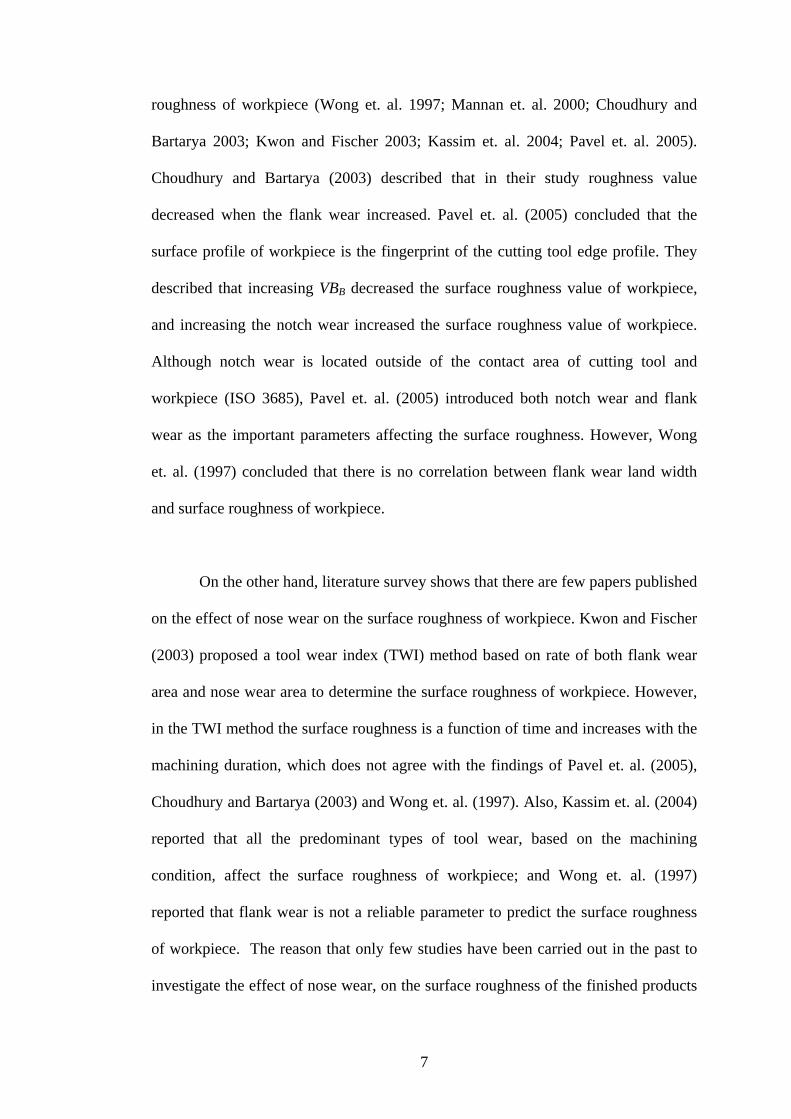
roughness of workpiece (Wong et. al. 1997; Mannan et. al. 2000; Choudhury and
Bartarya 2003; Kwon and Fischer 2003; Kassim et. al. 2004; Pavel et. al. 2005).
Choudhury and Bartarya (2003) described that in their study roughness value
decreased when the flank wear increased. Pavel et. al. (2005) concluded that the
surface profile of workpiece is the fingerprint of the cutting tool edge profile. They
described that increasing VBB decreased the surface roughness value of workpiece,
and increasing the notch wear increased the surface roughness value of workpiece.
Although notch wear is located outside of the contact area of cutting tool and
workpiece (ISO 3685), Pavel et. al. (2005) introduced both notch wear and flank
wear as the important parameters affecting the surface roughness. However, Wong
et. al. (1997) concluded that there is no correlation between flank wear land width
and surface roughness of workpiece.
On the other hand, literature survey shows that there are few papers published
on the effect of nose wear on the surface roughness of workpiece. Kwon and Fischer
(2003) proposed a tool wear index (TWI) method based on rate of both flank wear
area and nose wear area to determine the surface roughness of workpiece. However,
in the TWI method the surface roughness is a function of time and increases with the
machining duration, which does not agree with the findings of Pavel et. al. (2005),
Choudhury and Bartarya (2003) and Wong et. al. (1997). Also, Kassim et. al. (2004)
reported that all the predominant types of tool wear, based on the machining
condition, affect the surface roughness of workpiece; and Wong et. al. (1997)
reported that flank wear is not a reliable parameter to predict the surface roughness
of workpiece. The reason that only few studies have been carried out in the past to
investigate the effect of nose wear, on the surface roughness of the finished products

8
e.g. Kwon and Fischer (2003) can be due to the limitation of the existing methods,
which cannot measure the nose wear fast and accurately. Indirect methods such as
cutting force monitoring and vibration signatures give the signals that are
combination of effect of different types of tool wear on surface quality of workpiece.
Thus, the indirect methods cannot be used to study the effect of nose wear on the
surface quality alone. Also, Lanzetta (2001) indicated that vision system introduced
in the past cannot precisely be used to measure the nose wear of cutting tool using
simple subtraction methods. Thus, a method that is precise and fast has to be
introduced to assess the effect of nose wear on the surface quality of workpiece.
1.4 Problem statement
In the industries two important problems must be solved. The first is
evaluation the quantity of parameters that gives the desirable output. The second is
increase of the productivity of system. One important solution to solve theses two
problems is the use of models based on scientific background (Benardos and
Vosniakos 2003). The problems that based on the literatures were focused on them in
this study are as follows:
1.4.1 Effect of nose wear on the surface quality of workpiece
The nose radius area and minor cutting edge together shape the surface
profile of workpiece in a turning operation (ISO 3685, 1993). Thus, the tool wear
type that affects the nose radius area also affects the surface quality of workpiece.
The nose wear is one important type of tool wear that occurs in nose area of cutting
tool, thus affecting the surface quality of the product. However, study on the effect of
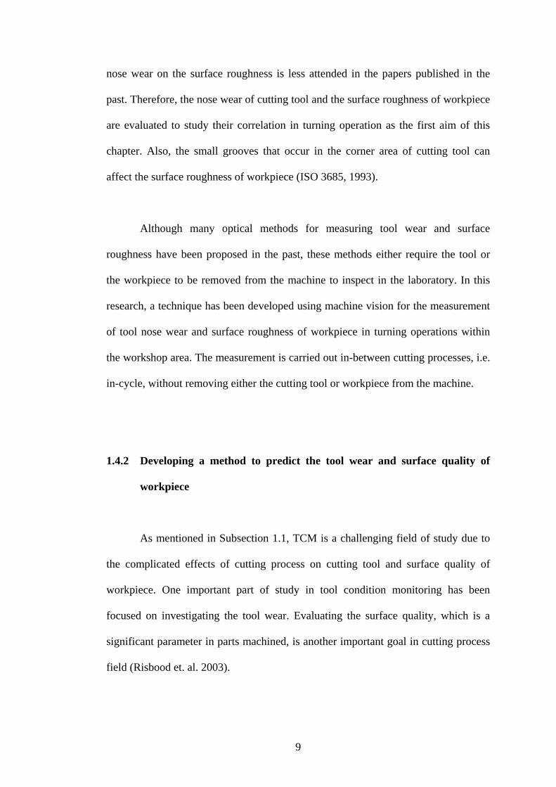
9
nose wear on the surface roughness is less attended in the papers published in the
past. Therefore, the nose wear of cutting tool and the surface roughness of workpiece
are evaluated to study their correlation in turning operation as the first aim of this
chapter. Also, the small grooves that occur in the corner area of cutting tool can
affect the surface roughness of workpiece (ISO 3685, 1993).
Although many optical methods for measuring tool wear and surface
roughness have been proposed in the past, these methods either require the tool or
the workpiece to be removed from the machine to inspect in the laboratory. In this
research, a technique has been developed using machine vision for the measurement
of tool nose wear and surface roughness of workpiece in turning operations within
the workshop area. The measurement is carried out in-between cutting processes, i.e.
in-cycle, without removing either the cutting tool or workpiece from the machine.
1.4.2 Developing a method to predict the tool wear and surface quality of
workpiece
As mentioned in Subsection 1.1, TCM is a challenging field of study due to
the complicated effects of cutting process on cutting tool and surface quality of
workpiece. One important part of study in tool condition monitoring has been
focused on investigating the tool wear. Evaluating the surface quality, which is a
significant parameter in parts machined, is another important goal in cutting process
field (Risbood et. al. 2003).

10
The large number of published work in the field of tool wear and effect of
tool wear on the surface quality revealed that introducing a certain method to solve
all problems in this field is difficult. This can be due to the complicated interaction
between cutting tool, workpiece and machine tool used.
However, detecting the cutting process using on-line and in-cycle monitoring
of tool wear is an applicable method to assess the stability of machining, increase
productivity, improve the surface quality of workpieces and decrease the unpredicted
parameters that can damage the machine tool (Dimla 2000). This means that using a
suitable TCM method can increase the productivity of production system (Bradley
and Wong 2001).
Rehorn et. al (2005) reviewed about 100 published work on TCM and
concluded that the future TCM methods have to be accurate, simple to carry out,
easy to install and maintain. Rehorn et. al. (2005) also suggested that advance
statistical methods can increase the efficiency of TCM method used. However,
replacing the worn out cutting tool just in time is not easy due to the complicated
phenomenon of tool wear as a complex process, which is a combination of abrasive,
adhesive and diffusive types of wear (Tay et. al. 2002). Therefore, it is essential to
focus on developing a system for TCM and surface quality assessment of workpiece
that is simple to carry out and flexible to implement in different cutting conditions.
As mentioned in Subsection 1.2, indirect methods are capable to be used on-
line and this is the significant advantage of these methods. However, these methods

11
are not easy to be implemented because evaluation of some of unpredicted signals
received from cutting process is difficult (Sortino 2003).
Compared to indirect methods, machine vision systems, which can assess the
cutting process directly, are suitable for investigating the cutting process directly.
These methods are fast and can easily recognize different types of tool wear.
Although these methods are able to measure the wear area precisely, vision systems
are sensitive to some ambient parameters such as particle dust, ambient disturbance
and light intensity (Lanzetta 2001). Also, they cannot be used to measure the wear
area when the machining process continues. This is because the wear area of cutting
tool is blocked by the chips formed during machining. This setback prevents the
implementation of machine vision systems in-process, and most of published
literatures using vision methods to monitor the tool wear are either off-line or in-
cycle i.e. between cutting cycles. These limitations show that it is necessary to
introduce a new algorithm in order to improve the in-process or in-cycle monitoring
methods of tool wear.
1.5 Objectives
The objectives of this study are as follows:
1. Measure of tool nose wear and flank wear, surface roughness and
dimensional deviation of workpiece developing a machine vision.
2. Study on the effect of nose wear on the surface roughness of turned parts.

12
3. Prediction of surface roughness and dimensional deviation of workpiece and
flank wear using a response surface method (RSM).
1.6 Research scope
The scopes and approaches of his research are as follows:
• Develop a 2-D vision method using image processing to decrease the
effect of ambient factors on results of TCM e.g. ambient lighting, ambient
vibration, micro dust particles and misalignment of cutting tool.
• Develop a 2-D vision method to measure the nose wear area of cutting
tool.
• Develop a 2-D vision method to measure the surface roughness of turned
parts.
• Study on the effect of nose wear on the surface roughness of parts
machined in turning operation.
• Evaluating the flank wear land width in nose area of cutting tool (VBC)
using top 2-D image of cutting tool.
• Develop a 2-D vision method to measure the dimensional deviation of
turned parts.
• Simulation of the surface profile of workpieces using the 2-D images of
cutting tools.
• Develop a DOE method to predict the surface roughness and dimensional
deviation of turned parts.

13
1.7 Outline of thesis
The thesis is organized to fulfill the objectives mentioned in Section 1.5 as
follows:
• Chapter 1 describes the background on the importance of cutting process,
importance of the TCM methods and problem being investigated. Also, in
Chapter 1 the objectives and the scopes of this work are introduced.
• In Chapter 2, past literatures published in TCM and prediction of the
effect of tool wear on surface quality, using direct methods and indirect
methods, are reviewed.
• In Chapter 3, the algorithms used to fulfill the objectives of this study are
described.
• In Chapter 4, the results of this study is presented and discussed.
• In Chapter 5, the conclusion of this thesis is made. Also, the
recommendations and suggestions for future study on the effect of tool
nose wear on the surface roughness of workpiece in turning operation are
given.
14
Chapter 2
Literature review
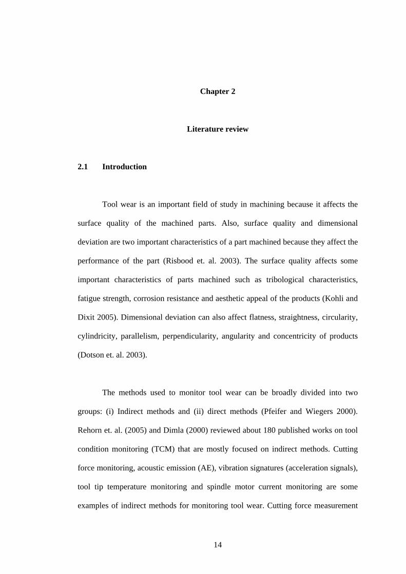
2.1 Introduction
Tool wear is an important field of study in machining because it affects the
surface quality of the machined parts. Also, surface quality and dimensional
deviation are two important characteristics of a part machined because they affect the
performance of the part (Risbood et. al. 2003). The surface quality affects some
important characteristics of parts machined such as tribological characteristics,
fatigue strength, corrosion resistance and aesthetic appeal of the products (Kohli and
Dixit 2005). Dimensional deviation can also affect flatness, straightness, circularity,
cylindricity, parallelism, perpendicularity, angularity and concentricity of products
(Dotson et. al. 2003).
The methods used to monitor tool wear can be broadly divided into two
groups: (i) Indirect methods and (ii) direct methods (Pfeifer and Wiegers 2000).
Rehorn et. al. (2005) and Dimla (2000) reviewed about 180 published works on tool
condition monitoring (TCM) that are mostly focused on indirect methods. Cutting
force monitoring, acoustic emission (AE), vibration signatures (acceleration signals),
tool tip temperature monitoring and spindle motor current monitoring are some
examples of indirect methods for monitoring tool wear. Cutting force measurement

15
and vibration signals method are two of the indirect methods used widely to evaluate
the tool wear in batch production (Dimla 2000). Indirect methods are capable for on-
line use to assess the tool wear, and this advantage is the reason for their wide
application (Sortino 2003). The basis of indirect methods is comparison between the
received signals from the current cutting process and the optimized signal as the
threshold. However, evaluation of signals received from indirect methods is not
simple because of the unpredicted parameters that can affect the output signals
(Pfeiffer and Wiegers 2000).
On the other hand, machine vision systems are well known as the direct
methods of TCM. Some studies on tool wear using vision systems were reported by
Kurada and Bradley (1997 b). The vision systems are suitable for assessing the tool
wear and surface quality of workpiece. The vision systems are also able to recognize
the tool wear pattern in different cutting process directly.
This chapter aims to survey the literatures focused on TCM and prediction of
effect of tool wear on the surface quality of products using direct and indirect
methods. In Section 2.2 the important types of tool wear are reviewed. Section 2.3
briefly discusses some early studies on TCM methods, Sections 2.4 and 2.5 discuss
about TCM using indirect and direct methods respectively, and Section 2.6 discusses
about some indirect and direct methods employed to predict the surface roughness
and dimensional deviation of workpiece.

16
2.2 Important types of tool wear
The important types of tool wear are flank wear, nose wear, crater wear and
notch wear as shown in Figures 2.1(a)-(b). Most of studies on TCM in the past have
been focused on flank wear and crater wear. This can be due to the recommendation
of ISO 3685 (1993) standard that introduced the flank wear and crater wear as the
criteria of tool life.
Figure 2.1. (a) Top view of crater wear and nose profile and (b) flank wear land and
notch wear of cutting tool based on ISO 3685 (1993).
When the relief face of a cutting tool rubs against the workpiece, flank wear
is created on this face. Therefore, this type of tool wear is made by an abrasion
mechanism. Flank wear decreases the accuracy of the parts machined because it
causes deflection of the cutting tool (Stephenson and Agapiou 1997). Flank wear
land width (VBB) shown in Figure 2.1(b) is the criterion of tool life. When the wear
Crater wear
Nose profile of new cutting
Nose profile of worn cutting tool D
epth
of c
ut
N
B
C
A
VBC
VBB max
VBA
VBB
Notch wear
VBN
Flank wear land
(a) (b)

17
patterns formed on relief face of cutting tool are regular, VBB =0.3 mm is the
criterion of tool life, and if the wear patterns formed on relief face of cutting tool are
not regular, VBB max=0.6 mm is the criterion of tool life.
Crater wear is another important type of tool wear that forms a rake on the
cutting tool face. This rake can be produced by chemical reaction or metal diffusion
due to high temperature on cutting tool face. Although crater wear increases the
effective angle of cutting tool that can decrease the cutting force, severe crater wear
makes the cutting tool weak.
Notch wear is produced by chemical reaction between cutting tool faces and
coolant or atmosphere (Stephenson and Agapiou 1997). When notch wear grows on
the cutting tool face, it can cause breakage of the cutting tool due to the grooves
produced on the tool tip that weakens the cutting tool structure. Therefore, according
to ISO 3685 (1993) severe notch wear is also a criterion of tool life. In this case, the
notch wear width VBN = 0.3 mm is the criterion of tool life when the cutting tool is
regularly worn on the relief face. On the other hand, if the cutting tool is not
regularly worn on the relief face, the cutting tool shall be replaced when VBN exceeds
0.6 mm.
Nose area of cutting tool is where the nose wear occurs. When severe nose
wear is formed catastrophic tool failure can occur (Dimla 2000). Nose wear is a
combination of flank wear and notch wear (Jurkovic et. al. 2005, Stephenson and
Agapiou 1997). Figure 2.1(a) shows the nose wear, which consists of flank wear and
notch wear, as the important type of tool wear. Kwon and Fischer (2003) reported

18
that the nose wear affects the surface quality of workpiece in turning operation. This
finding agrees with ISO 3685 (1993) standard that introduced the tool corner radius
as one of the main factors that affects the surface roughness of workpiece in a
turning operation.
2.3 Overview of the methods of TCM and early studies
There are a number of different methods used to evaluate tool wear. These
methods can be grouped into two general groups:
• Indirect methods
• Direct methods
Vibration signatures (acceleration signals), cutting force monitoring, acoustic
emission (AE), tool tip temperature monitoring and spindle motor current are some
examples of indirect methods of tool wear monitoring. Among these, vibration
signals and cutting force measurement methods are used widely to evaluate the
cutting process in batch production (Dimla 2000). Indirect methods are capable to be
used on-line to assess tool wear (Pfeifer and Wiegers 2000). This advantage has
encouraged the industries to adopt some of these methods. The indirect methods are
based on comparison between the received signal of current cutting process and
optimized signal of cutting process. When the received signals are out of optimized
signal bound, the system will send a signal to change the cutting tool (Pfeifer and
Wiegers 2000). Thus, the threshold signals must be investigated before using these
methods to monitor the cutting process.
19
Although indirect methods based on vibration signals and cutting force
signals have been used widely for TCM, Sortino (2003) reported that it is not simple
to design the indirect methods to apply in a real condition. This can be due to lack of
knowledge about some signals received from the cutting process using indirect
methods. In addition, these methods are costly to monitor the cutting process because
they are complex and are not simple enough to use in a workshop easily (Sortino
2003, Pfeifer and Wiegers 2000).
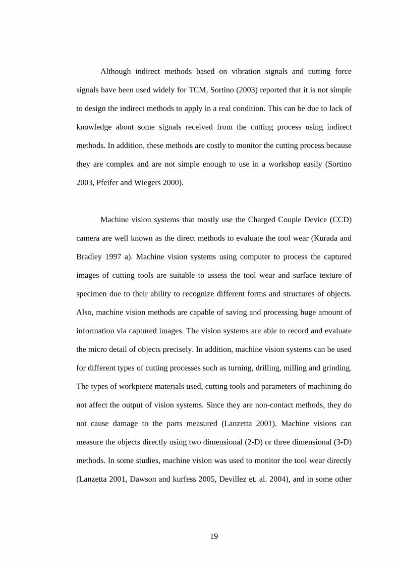
Machine vision systems that mostly use the Charged Couple Device (CCD)
camera are well known as the direct methods to evaluate the tool wear (Kurada and
Bradley 1997 a). Machine vision systems using computer to process the captured
images of cutting tools are suitable to assess the tool wear and surface texture of
specimen due to their ability to recognize different forms and structures of objects.
Also, machine vision methods are capable of saving and processing huge amount of
information via captured images. The vision systems are able to record and evaluate
the micro detail of objects precisely. In addition, machine vision systems can be used
for different types of cutting processes such as turning, drilling, milling and grinding.
The types of workpiece materials used, cutting tools and parameters of machining do
not affect the output of vision systems. Since they are non-contact methods, they do
not cause damage to the parts measured (Lanzetta 2001). Machine visions can
measure the objects directly using two dimensional (2-D) or three dimensional (3-D)
methods. In some studies, machine vision was used to monitor the tool wear directly
(Lanzetta 2001, Dawson and kurfess 2005, Devillez et. al. 2004), and in some other

20
studies machine vision was used to evaluate the cutting tool condition via surface
texture (Mannan et. al. 2000, Kassim et. al. 2004).
Lighting is an important factor in all machine vision applications. The type of
illumination used depends on the output required. There are two main types of
lighting:
• Front-lighting
• Back-lighting
In front-lighting method, both of illumination source and camera are in front
of the specimen. The output of this method is an image of the object surface. When
the specimen is placed between camera and the source of light, this method is called
back-lighting. Back-lighting is used when it is necessary to capture an image of
specimen contour. Front-lighting is the method used to study the flank wear (Pfeifer
and Wiegers 2000; Kurada and Bradley 1997 a), crater wear (Prasad and
Ramamoorthy 2001; Dawson and Kurfess 2005) and their effect on surface
roughness (Mannan et. al. 2000, Kassim et. al. 2004). Meanwhile back-lighting is the
method which has been used to measure the nose wear in off-line mode (Kwon and
Fischer 2003).
This research aims to study the effect of nose wear, which is located on the
profile of cutting tool, on surface roughness using direct methods that was not
studied in the past. Thus, the back-lighting method, which is a suitable method to use

21
to capture the images of tool contour, was employed to assess the tool wear of
cutting tool.
According to literature survey in this study, the effect of cutting speed on tool
life of cutting tool was one of the earliest studies reported in the field of metal
cutting process. The study carried out by Taylor (1907) showed that the effect of
cutting speed on tool life is significant and the manufacturer has to use the optimum
cutting speed. The cost of tooling and downtime of machining can be decreased
using the optimum cutting speed. The optimum cutting speed V is given by:
TnCV logloglog −= (2.1)
i.e. CVT n = (2.2)
where T is cutting time to produce a standard flank wear land width (e.g. 0.6 mm for
irregular wear pattern on the relief face). C and n are constant of material and
machining condition respectively.
Since access to the very old work published in the field of tool wear in
cutting process was not easy, the literature survey on the history of tool wear in this
work is not comprehensive. However, the published works that are introduced in this
section shows the trend of study in cutting process. The trend shows that the goal of
these studies were focused on understanding the effect of machining parameters on
the tool wear that affects the machined parts and productivity. Since the cutting
speed is not the only parameter that has to be observed to increase the product
22
quality and decrease the tool wear rate, other investigators followed Taylor’s method
to study on the other important parameters of machining. Some of these studies are
briefly described in this section. Hake (1955) proposed a method based on
radioactive γ ray to measure the effect of wear on the cutting tool. Shaw and Dirke
(1956) studied on the nature of wear pattern of the cutting tool to understand the
effect of wear on the tool life of cutting tool. Taylor (1957) suggested using the area
of tool wear to improve the accuracy of measuring the wear pattern.
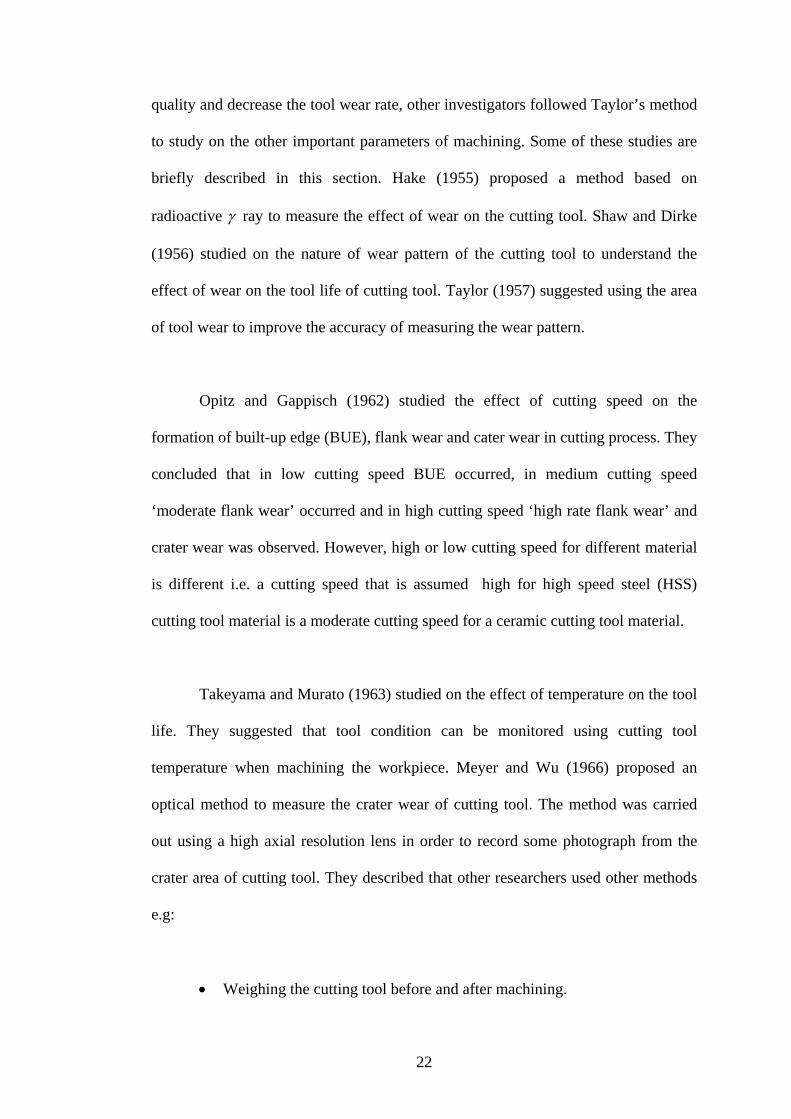
Opitz and Gappisch (1962) studied the effect of cutting speed on the
formation of built-up edge (BUE), flank wear and cater wear in cutting process. They
concluded that in low cutting speed BUE occurred, in medium cutting speed
‘moderate flank wear’ occurred and in high cutting speed ‘high rate flank wear’ and
crater wear was observed. However, high or low cutting speed for different material
is different i.e. a cutting speed that is assumed high for high speed steel (HSS)
cutting tool material is a moderate cutting speed for a ceramic cutting tool material.
Takeyama and Murato (1963) studied on the effect of temperature on the tool
life. They suggested that tool condition can be monitored using cutting tool
temperature when machining the workpiece. Meyer and Wu (1966) proposed an
optical method to measure the crater wear of cutting tool. The method was carried
out using a high axial resolution lens in order to record some photograph from the
crater area of cutting tool. They described that other researchers used other methods
e.g:
• Weighing the cutting tool before and after machining.

23
• Measuring the depth of crater wear using the stylus method.
• Gradual lapping down of top surface of crater wear area.
• Use of radioactive isotopes method.
The results showed that the proposed method, which is an optical method,
could successfully be used to measure the depth of crater wear.
Mukherjee and Basu (1966) used a regression method in order to model the
effect of machining variables on the flank wear. The variables used in this study
were: Duration of machining, feed rate, cutting speed and depth of cut. The output
response was flank wear that was measured using a toolmaker’s microscope. The
results showed that regression method can be used to model the effect of machining
parameters on the flank wear. Also, they concluded that cutting speed affected the
flank wear rate significantly.
Bhattacharyya and Ham (1969) proposed a mathematical method to model
the flank wear. They varied some different machining parameters to model the
mechanism of forming the wear pattern on the relief face of cutting tool. The
parameters varied were: Cutting tool material, cutting tool angle and duration of
machining. The parameters that were kept constant were: Cutting speed, depth of cut,
feed and workpiece material. They concluded that the proposed method could
effectively be used in similar machining conditions. Thus, modeling the flank wear
rate is not possible using machining condition that is different from the experiments
carried out.

24
Bhattacharyya and Gonzalez (1970) proposed a regression model to predict
the surface roughness and determine the optimum machining condition. The
variables used were: Feed rate, cutting speed, length of workpiece to be machined,
diameter of workpiece and tool life. The method used was successful in predicting
the surface roughness and optimizing the machining process in the known field of
variables.
Sundram (1978) proposed a method to predict the surface roughness of
workpiece. Also, the model constructed was used to determine the optimum
machining conditions. The variable parameters chosen were: Surface roughness
value, power consumption of machine tool used, cutting speed, feed rate and depth
of cut while other machining parameters were fixed. A relatable design method,
which is a type of statistical DOE method, was used to design the experiments. A
stepwise regression method was also used to analyze the data obtained from
machining process. Sundram concluded that the goals of proposed study were
fulfilled using the proposed method successfully. Thus, Sundram suggested using the
concept of proposed method to solve the similar problems using machining condition
that is desirable.
Tlusty and Massod (1978) studied on the chipping and fracture of cutting tool
as the catastrophic types of tool failure. They used two methods to study the tool
failure: A plain stress-strain analyses method and fractographic method. However,
they mentioned that due to neglecting some other parameters such as effect of
temperature on the output, this method cannot be mentioned absolute.