Embed Size (px)
Citation preview
Studying protein-ligand binding by spectroscopy and
calorimetry
Erick Alejandro Meneses Ramirez
Degree of Doctor of Philosophy
Department of Chemistry
McGill University
Montreal, Quebec, Canada
August 2014
A Thesis submitted to McGill University in partial fulfillment of the requirements
for the degree of Doctor of Philosophy
© Erick Meneses, 2014 all rights reserved
i
Abstract
Different molecular, thermodynamic, and kinetic aspects of protein-ligand
binding were studied in the present thesis. This was accomplished using
diverse techniques such as Nuclear Magnetic Resonance (NMR),
fluorescence spectroscopy, and calorimetry.
Chapter 1 introduces the basic concepts to understand the dynamics and
thermodynamics of binding for systems where a ligand receives just one
binding molecule.
Chapter 2 gives an up-to-date technical background on NMR experimental
techniques to study dynamics and thermodynamics of protein-ligand
binding. These techniques were key to the research developed in chapters
3, 4 and to a lesser extent in Chapter 5.
Chapters 3 and 4 focused on the interaction between the Fyn SH3 domain
and several proline rich peptides. Chapter 3 describes the role of
electrostatic interactions in the binding pathway of transient protein
complexes formed by the SH3 domain and three proline-rich peptides. We
showed that the electrostatic enhancement of binding for this weak (≥µM
KD), short-lived complex with lifetimes on the order of milliseconds is much
less, and basal association rates are greater than those previously
observed for tight (<nM KD) long-lived systems with lifetimes on the order
of minutes or longer. This suggests that electrostatics may play different
roles in short-lived and long-lived protein complexes.
Chapter 4 mapped the changes in volume for the association pathway for
the Fyn SH3 domain and a proline rich peptide. Via pressure we were able
ii
to quantify changes in molar volume between the free, bound and
transition states for this system. This is, to our knowledge, the first
measurement of the activation volume for a protein-ligand binding reaction.
The results agree with a protein-ligand binding pathway involving
significant desolvation of the binding surfaces. We found that the volume
of transition state is very close to that of the fully bound state. This
suggests that the rearrangement of solvating water molecules and protein
and ligand and conformational changes occur before the transition state.
Chapter 5 explored different NMR experimental approaches for studying
the interaction between bisphophonate inhibitors and human farnesyl
pyrophosphate synthase. Different isotopic protein labeling patterns were
used to study this system together with a series of NMR experiments
designed to exploit these specifically labeled proteins.
iii
Résumé
Dans cette thèse nous avons étudié plusieurs aspects de biologie
moléculaire, de thermodynamique, et de cinétique chimique liés aux
processus d'union entre une protéine et son ligand. Afin de mener ces
études, diverses techniques telles que la Résonance Magnétique
Nucléaire (RMN), la spectroscopie de fluorescence et la calorimétrie ont
été utilisées.
Le premier chapitre introduit les concepts de base afin de comprendre la
dynamique et la thermodynamique d'union entre protéines. Un modèle
simplifié dans lequel une protéine joint seulement un ligand sera utilisé.
Le deuxième chapitre donne une mise à jour des techniques RMN
récentes que l'on peut utiliser pour étudier la thermodynamique et la
cinétique d'union d'une protéine avec son ligand. Ces techniques sont
cruciales pour développer les travaux de recherche expliqués dans les
chapitres 3, 4 et d’une manière plus limitée dans le chapitre 5.
Le troisième et quatrième chapitres traitent de l'interaction entre le
domaine d'union SH3 de la tyrosine kinase fyn et plusieurs peptides riches
en prolines. Nous avons démontré que l'influence des forces
électrostatiques dans la constante de vitesse est plus faible pour les
systèmes ayant un temps de demi-vie de l'ordre de la milliseconde et
iv
possèdent des faibles constantes d'affinités (≥µM KD) par rapport aux
complexes plus stables, avec un temps de demi-vie de l'ordre d’heures ou
de jours, qui possèdent constantes d'affinités plus élevées (<nM KD). Nous
avons également démontré que les vitesses d'association basales,
indépendantes des forces électrostatiques, sont plus importantes dans la
formation de complexes transitoires. Cela suggère que les forces
électrostatiques jouent un rôle différent dans les complexes transitoires et
les complexes stables.
Le quatrième chapitre cartographie les changements de volume pour
l'association entre le domaine SH3 et un peptide riche en prolines. En
utilisant la pression hydrostatique nous avons mesuré les volumes
molaires relatifs de l'état libre, l'état de transition et du complexe final
protéine-ligand uni. D'après nous, c'est la première fois que le volume
d'activation pour un processus d'union entre protéines est mesuré. Les
résultats sont en accord avec une libération d'eau d'hydratation des
surfaces d'union entre la protéine et le peptide. Nous avons observé que le
volume de l'état de transition est très proche de celui du complexe final.
Dans le cinquième chapitre différentes approches expérimentales de RMN
ont été explorées afin d’étudier l'interaction entre les inhibiteurs type
bisphosphonates et la protéine humaine farnesyl pyrophosphate synthase.

v
Différents systèmes de marquage isotopique de la protéine ont été
essayés afin d’étudier cette interaction.
vi
Acknowledgments
First and foremost I would like to thank my supervisor Dr. Anthony
Mittermaier for his support and guidance during my Ph. D. studies. He took
an extremely shy and confused individual at the beginning of his graduate
studies, and patiently, he was able to guide me in becoming someone who
is a little less shy and at least a little bit more able to do some research.
Dr. Tara Sprules was also an unconditionally kind and always opportune
voice of support while I was learning (as I always will be) all the
instrumental tools as an NMR spectroscopist. Thank you so much for all
the patience and careful explanation of NMR experiments.
I would also like to thank all of the evaluation committee members
throughout my studies: Professors Amy S. Blum, Gonzalo Cosa, Nicolas
Moitessier, and Masad Dahma. Annual discussions on research were
always an interesting time for learning.
I would like to thank Jean-Philippe Demers. Hardworking craziness is
perhaps the best way to learn about biological NMR from someone who is
an outstanding researcher.

vii
I wish to acknowledge my friend and lab mate Pierre Karam for his always
nice voice of support and his endless corridor planed jokes. Also I wish to
thank all the actual and past lab members, Pat, Lee, Teresa, Jason, Eric H,
Siqi, Stephane, Rob H., Justin, and Eric. They made my journey through
graduate studies more pleasant.
Finally I would like to thank to the three more important people in my life.
My always supportive Mother Flor Marina, my wife Andrea, who changed
her professional, nice and comfortable life in Colombia to come over to
Canada to follow our dreams. Thank you Andrea for bringing that little
piece of joy and cuteness that is healthy growing inside you.
viii
Table of Contents
Abstract ................................................................................................................................. i Résumé .............................................................................................................................. iii Acknowledgments .............................................................................................................. vi Table of Contents. ............................................................................................................ viii List of Figures ..................................................................................................................... xi List of Tables .................................................................................................................... xiv Abbreviations ..................................................................................................................... xv 1. Introduction ...................................................................................................................... 1
1.1 Importance of studying protein-ligand binding ......................................................... 2 1.2 Rigid two-body binding ............................................................................................. 4 1.3 Binding equilibrium constants in a system exchanging between two states ............ 6 1.4 Protein-ligand dynamics ......................................................................................... 10 1.5 Protein ligand binding limited by diffusion .............................................................. 16 1.6 Association rate constants kon and transition state ................................................ 21 1.7 Relation between diffusion coefficient and viscosity .............................................. 24 1.8 Measuring protein-ligand binding thermodynamics ................................................ 28
1.8.1 Isothermal Titration Calorimetry, model for 1:1 binding ................................. 29 1.8.2 Intrinsic tryptophan Fluorescence and protein ligand binding ........................ 31
1.9.Biological systems .................................................................................................. 33 1.9.1 Protein interaction domains ............................................................................ 34 1.9.2 Proline rich motifs and polyproline II conformation ........................................ 35 1.9.3 Fyn SH3 ......................................................................................................... 36 1.9.4 hFPPS ............................................................................................................ 38
2. Analyzing Protein-Ligand Interactions by Dynamic NMR Spectroscopy ....................... 41
2.1 Summary ................................................................................................................ 42 2.2 Introduction ............................................................................................................. 43 2.3 Materials ................................................................................................................. 51
2.3.1 NMR samples ................................................................................................. 51 2.3.2 Spectral Analysis ............................................................................................ 53
2.4 Methods .................................................................................................................. 55 2.4.1 Titration analysis ............................................................................................ 55
2.4.1.1 NMR-derived binding isotherms .......................................................... 55
ix
2.4.1.2 Line-shape analysis ............................................................................. 58 2.4.2 Carr-Purcell-Meiboom-Gill (CPMG) experiments ........................................... 61
2.4.2.1 CPMG overview ................................................................................... 61 2.4.2.2 CPMG data analysis ............................................................................ 65
2.4.3 Magnetization exchange spectroscopy (EXSY) ............................................. 70 2.4.3.1 EXSY overview .................................................................................... 70 2.4.3.2 EXSY data analysis ............................................................................. 72
2.5 Notes ...................................................................................................................... 75 2.5.1 NMR Titrations ............................................................................................... 75 2.5.2 CPMG experiments ........................................................................................ 76 2.5.3 EXSY experiments ......................................................................................... 79
3. Electrostatic interactions in the binding pathway of a transient protein complex studied by NMR and isothermal titration calorimetry ..................................................................... 80
3.1 Abstract .................................................................................................................. 81 3.2 Introduction ............................................................................................................. 82 3.3 Materials and methods ........................................................................................... 90
3.3.1 ITC .................................................................................................................. 90 3.3.2 NMR ............................................................................................................... 91 3.3.3 Electrostatic Enhancements ........................................................................... 95 3.3.4 Stopped-flow binding kinetics ......................................................................... 95 3.3.5 NMR-derived binding kinetics ........................................................................ 98
3.4 Results and discussion ........................................................................................... 99 3.4.1 NMR titration experiments .............................................................................. 99 3.4.2 Isothermal Titration Calorimetry ................................................................... 102 3.4.3 NMR kinetics experiments ........................................................................... 104 3.4.4 Comparison of NMR and stopped-flow binding kinetics .............................. 108 3.4.5 Electrostatic enhancement of association rates ........................................... 110 3.4.6 Arginine interactions in the transition state and bound state ....................... 115 3.4.7 Ionic strength dependence of dissociation rates .......................................... 118
3.5 Conclusions .......................................................................................................... 120 3.6 Acknowledgements. ............................................................................................. 122
4. Mapping volume changes in the binding pathway of an SH3 domain and a proline rich peptide ............................................................................................................................. 123
4.1 Summary. ............................................................................................................. 124
x
4.2 Introduction. .......................................................................................................... 126 4.3 Experimental ......................................................................................................... 131
4.3.1 Protein and peptide purification .................................................................... 131 4.3.2 Intrinsic tryptophan fluorescence experiments ............................................. 131 4.3.3 Changes upon binding in molecular volume ∆VM, thermal volume ∆VT, and measurement of accessible solvent surfaces for the free and bound states ........ 132 4.3.4 CPMG experiments ...................................................................................... 134
4.5 Results .................................................................................................................. 136 4.5.1 Intrinsic tryptophan fluorescence experiments ............................................. 136 4.5.2 Measurement of ∆VM, ∆VT and analysis of ∆VI ............................................ 141 4.5.3 CPMG NMR kinetic experiments ................................................................. 144
4.6 Conclusion ............................................................................................................ 147 5. NMR experimental approaches to study binding of bisphophonates to human Farnesyl Pyrophosphate Synthase (hFPPS) .................................................................................. 149
5.1 Overview. .............................................................................................................. 150 5.2 hFPPS expression and purification ...................................................................... 154 5.3 HSQC NMR experiments on hFPPS. ................................................................... 155 5.4 Further experiments on hFPPS ............................................................................ 158
5.4.1 Lysine methylation of hFPPS. ...................................................................... 162 5.4.2 hFPPS deuteration ....................................................................................... 166 5.4.3 . hFPPS perdeuteration and 1H-13C labeling of methyl groups on isoleucines, leucines and valines using metabolic precursors .................................................. 169
6. Further research directions .......................................................................................... 174
6.1 Overview ............................................................................................................... 175 6.2 Electrostatic interactions in the binding pathway of a transient protein complex studied by NMR and isothermal titration calorimetry. ................................................. 175 6.3 Mapping volume changes in the binding pathway of an SH3 domain and a proline rich peptide ................................................................................................................. 177 6.4 NMR experimental approaches to study binding of bisphophonates to human Farnesyl Pyrophosphate Synthase (hFPPS). ............................................................ 178
References ...................................................................................................................... 180
xi
List of Figures
Chapter 1 Figure 1.1 Cylinder containing a semi-permeable piston m .............................................. 24 Figure 1.2 Diffusion of a dissolved substance in a differential volume dx. ........................ 25 Figure 1.3 Human Fyn SH3 domain binding to peptide VSLARRPLPPLP ....................... 38 Chapter 2 Figure 2.1 Effect of ligand-binding on an NMR signal ....................................................... 46 Figure 2.2. Schematic representation of a 2D NMR 1H–15N correlation experiment ......................................................................................................................... 47 Figure 2.3 Titration monitored by heteronuclear correlation spectroscopy ....................... 50 Figure 2.4 Simulated binding isotherms ............................................................................ 56 Figure 2.5 Dissociation constant from a global analysis of 15N and 1H chemical shift displacements .................................................................................................................... 58 Figure 2.6 Schematic representation of a 15N CPMG experiment ................................... 64 Figure 2.7. Exchange rates from CPMG dispersion curves .............................................. 70 Figure 2.8 Schematic representation of an EXSY pulse sequence. ................................. 72 Chapter 3 Figure 3.1 Regions of 15N-1H HSQC spectra of the Fyn SH3 domain titrated with RR SR and SS peptides ................................................................................................................ 99 Figure 3.2 Structure of the Fyn SH3 domain in complex with a ligand identical to the RR peptide but containing Val rather than Trp at position -8, PDB 4EIK .............................. 100 Figure 3.3 Isothermal Titration Calorimetry raw thermograms and integrated heats for RR, SR and SS peptides binding to the Fyn SH3 domain at 40°C and different ionic strength. ......................................................................................................................................... 102 Figure 3.4 Base 10 logarithms of affinity constants, KA, of the Fyn SH3 domain for RR, SR, and SS peptides plotted as a function of ionic strength. .......................................... 103 Figure 3.5 NMR 15N CPMG relaxation dispersion data for the backbone amide signal of W36 collected at 500 and 800 MHz and 0M NaCl. ......................................................... 105 Figure 3.6 Comparison of 2 15N chemical shift parameters extracted from CPMG relaxation dispersion NMR experiments performed on the Fyn SH3 domain partially-
saturated with the RR peptide (0M NaCl) and 2 peak displacements from a comparison
of the Fyn SH3 domain spectra free and saturated with the RR peptide (0 M NaCl). .... 106
xii
Figure 3.7 Stopped-flow fluorescence data for the Fyn SH3 domain rapidly mixed with buffer and with a solution of the RR peptide. .................................................................. 109 Figure 3.8 Ionic strength dependence of association rates ............................................. 111 Figure 3.9 Enhancements in affinities (KASR,RR/KASS) and association rates (konSR,RR/konSS) for the RR and SR peptides relative to the SS peptide, plotted as a function of fion ....... 115 Chapter 4 Figure 4.1 Chicken Fyn SH3 domain intrinsic Trytophan fluoresence spectra ............... 137 Figure 4.2 r vs center of spectral mass for binding between chicken fyn SH3 domain and Ac-FSLARRPLPPLP-NH2 peptide. .................................................................................. 138 Figure 4.3 Change in free energy of binding as a function of pressure for the system chicken fyn SH3 domain/Ac-FSLARRPLPPLP-NH2 peptide ........................................... 140 Figure 4.4 Cavity volume calculations for the free and bound states using castP. ......... 142 Figure 4.5 Change in free energy between the bound state and the transition state as a function of pressure for the system chicken fyn SH3 domain / Ac-FSLARRPLPPLP-NH2 peptide. ............................................................................................................................ 145 Figure 4.6 Plot of |(∆δi)HSQC| vs |(∆ωi)CPMG| for every residue used to calculate kinetic parameters at every the pressures. ................................................................................. 146 Figure 4.7. Volume change map for binding between a chicken fyn SH3 domain and Ac-FSLARRPLPPLP-NH2 peptide ........................................................................................ 147 Chapter 5 Figure 5.1 Schematic representation of the mevalonate pathway. ................................. 151 Figure 5.2 The structure of some simple bisphophonates. ............................................. 152 Figure 5.3 1H-15N HSQC spectrum for the Apo form of hFPPS. ..................................... 156 Figure 5.4 1H-15N HSQC for 15N labeled hFPPS saturated with magnesium, the bisphophonate Zoledronate and pyrophosphate. ............................................................ 158 Figure 5.5 Reaction for 13C reductive methylation of lysines. ......................................... 164 Figure 5.6 1H-13C HSQC spectrum of hFPPS 13C lysine methylated in the apo state ... 165 Figure 5.7 1H-15N HSQC spectrum for a partially deuterated sample of hFPPS. ............ 168 Figure 5.8 1H-15N HSQC spectrum for a partially deuterated sample of hFPPS saturated with magnesium, Zoledronate and pyrophosphate ......................................................... 168 Figure 5.9 1H-15N spectrum TROSY-HSQC experiment for perdeuterated, methyl labeled hFPPS in the apo state. ................................................................................................... 171 Figure 5.10 shows a 1H-13C methyl HMQC experiment for a 300uM hFPPS in the apo state. ................................................................................................................................ 171
xiii
Figure 5.11 1H-13C methyl HMBC experiment of hFPPS perdeuterated and methyl labeled on ILV, saturated with magnesium, Zoledronate an pyrophospate .................... 173
xiv
List of tables
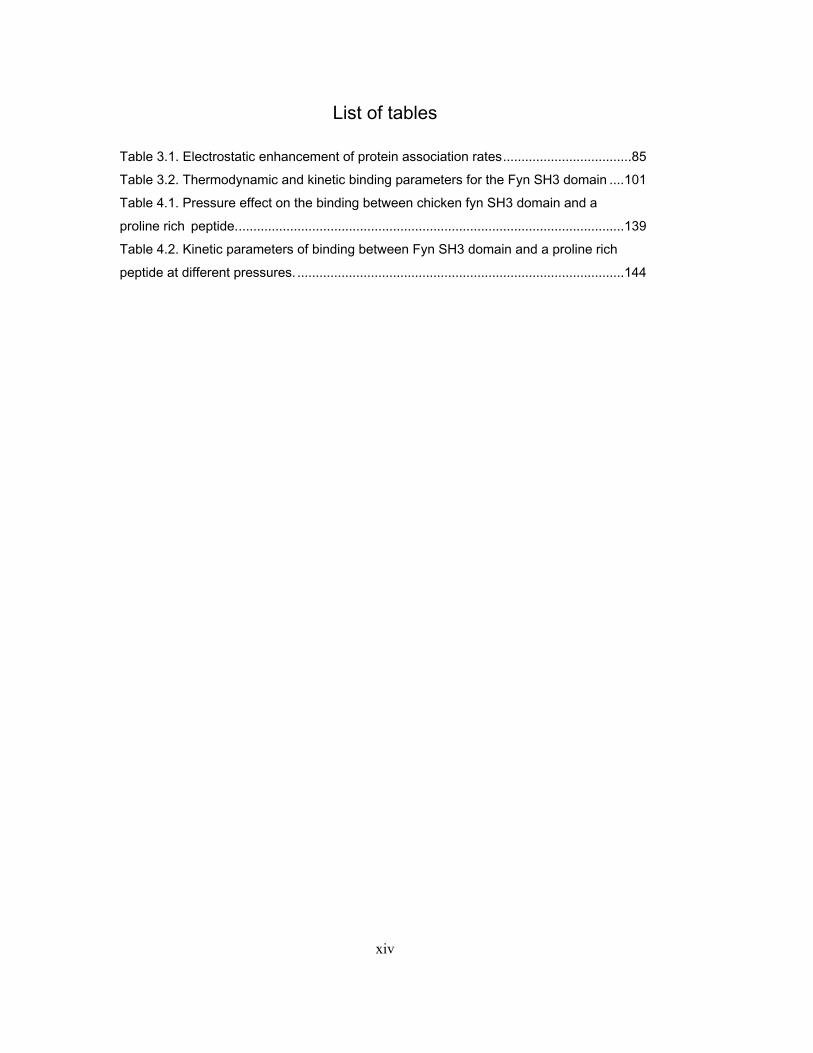
Table 3.1. Electrostatic enhancement of protein association rates ................................... 85 Table 3.2. Thermodynamic and kinetic binding parameters for the Fyn SH3 domain .... 101 Table 4.1. Pressure effect on the binding between chicken fyn SH3 domain and a proline rich peptide. ......................................................................................................... 139 Table 4.2. Kinetic parameters of binding between Fyn SH3 domain and a proline rich peptide at different pressures. ......................................................................................... 144
xv
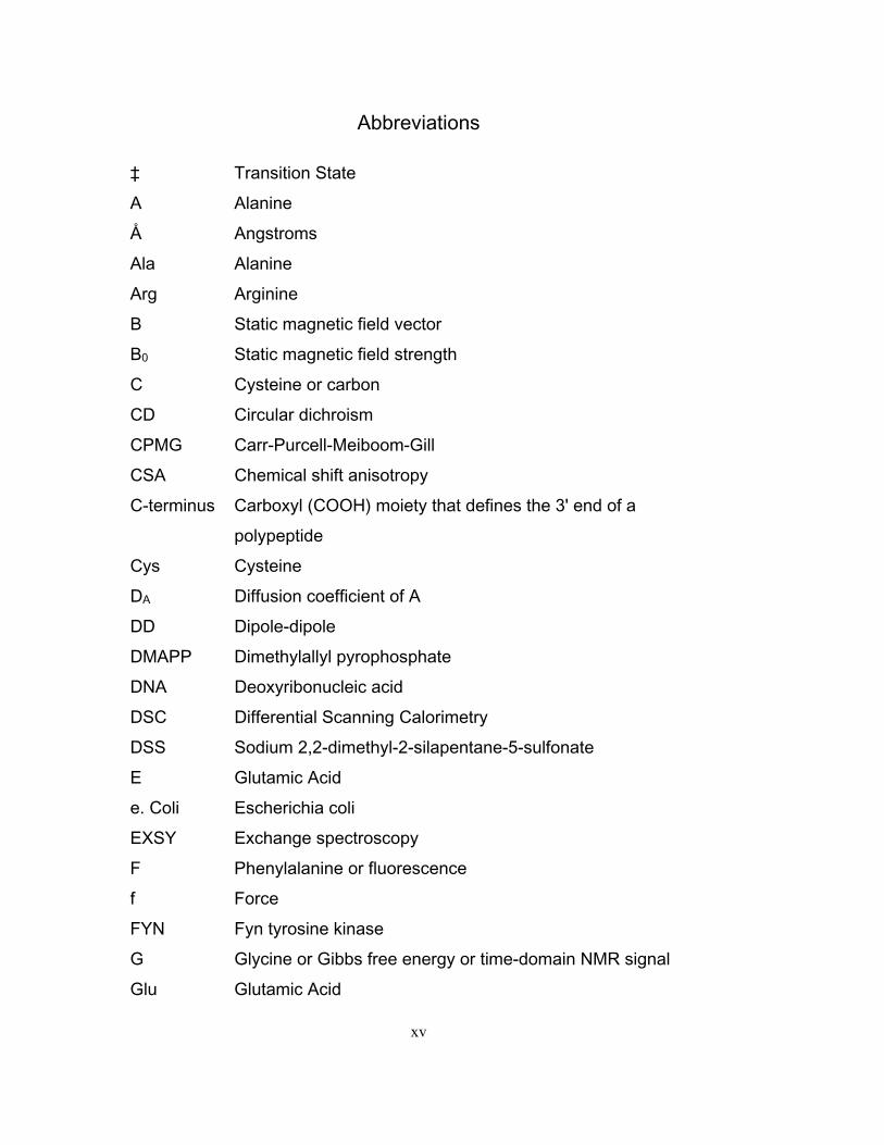
Abbreviations
‡ Transition State A Alanine Å Angstroms Ala Alanine Arg Arginine B Static magnetic field vector B0 Static magnetic field strength C Cysteine or carbon CD Circular dichroism CPMG Carr-Purcell-Meiboom-Gill CSA Chemical shift anisotropy C-terminus Carboxyl (COOH) moiety that defines the 3' end of a polypeptide Cys Cysteine DA Diffusion coefficient of A DD Dipole-dipole DMAPP Dimethylallyl pyrophosphate DNA Deoxyribonucleic acid DSC Differential Scanning Calorimetry DSS Sodium 2,2-dimethyl-2-silapentane-5-sulfonate E Glutamic Acid e. Coli Escherichia coli EXSY Exchange spectroscopy F Phenylalanine or fluorescence f Force FYN Fyn tyrosine kinase G Glycine or Gibbs free energy or time-domain NMR signal Glu Glutamic Acid
xvi
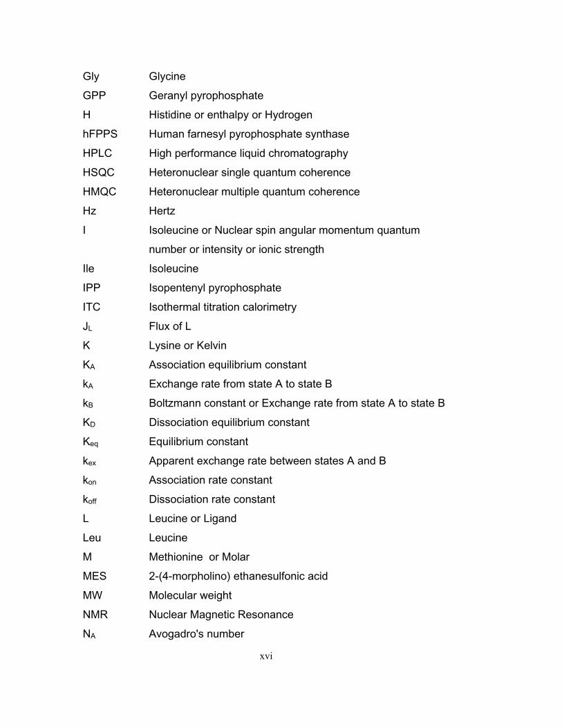
Gly Glycine GPP Geranyl pyrophosphate H Histidine or enthalpy or Hydrogen hFPPS Human farnesyl pyrophosphate synthase HPLC High performance liquid chromatography HSQC Heteronuclear single quantum coherence HMQC Heteronuclear multiple quantum coherence Hz Hertz I Isoleucine or Nuclear spin angular momentum quantum number or intensity or ionic strength Ile Isoleucine IPP Isopentenyl pyrophosphate ITC Isothermal titration calorimetry JL Flux of L K Lysine or Kelvin KA Association equilibrium constant kA Exchange rate from state A to state B kB Boltzmann constant or Exchange rate from state A to state B KD Dissociation equilibrium constant Keq Equilibrium constant kex Apparent exchange rate between states A and B kon Association rate constant koff Dissociation rate constant L Leucine or Ligand Leu Leucine M Methionine or Molar MES 2-(4-morpholino) ethanesulfonic acid MW Molecular weight NMR Nuclear Magnetic Resonance NA Avogadro's number
xvii
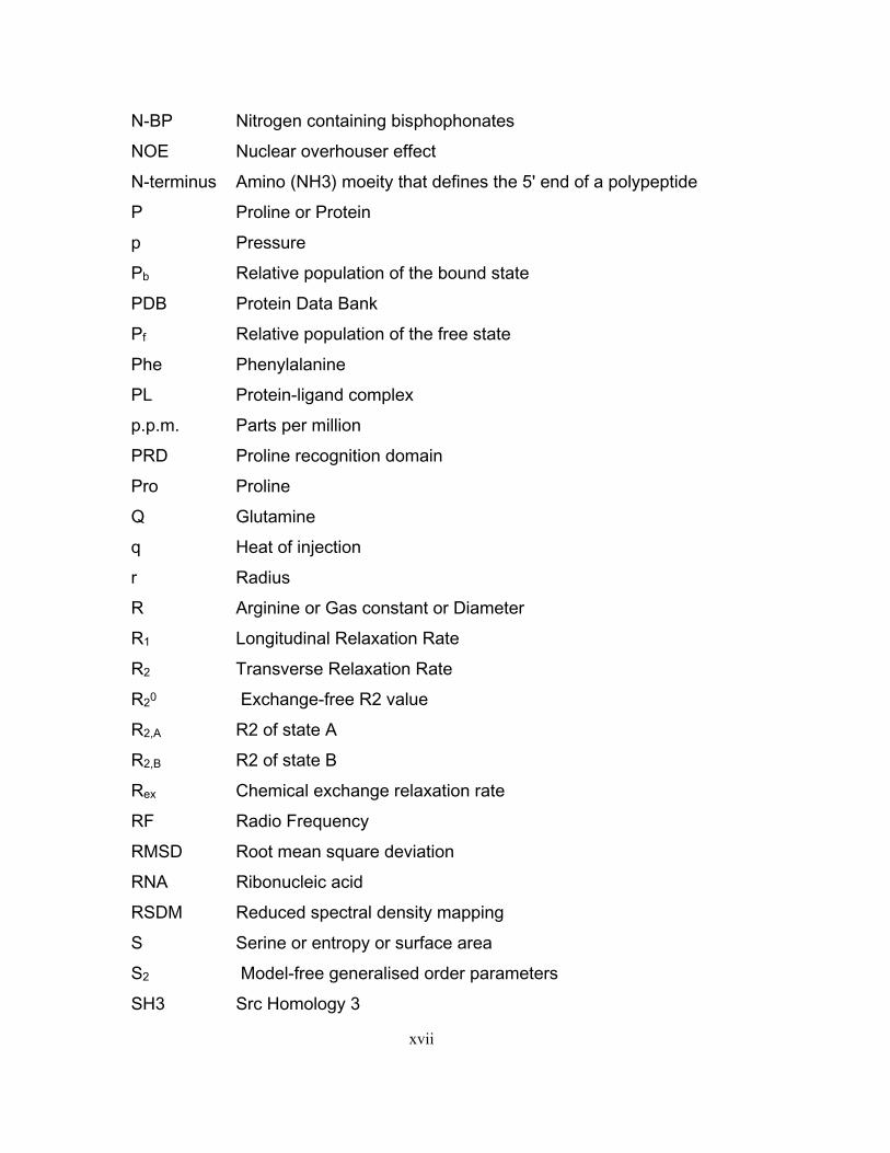
N-BP Nitrogen containing bisphophonates NOE Nuclear overhouser effect N-terminus Amino (NH3) moeity that defines the 5' end of a polypeptide P Proline or Protein p Pressure Pb Relative population of the bound state PDB Protein Data Bank Pf Relative population of the free state Phe Phenylalanine PL Protein-ligand complex p.p.m. Parts per million PRD Proline recognition domain Pro Proline Q Glutamine q Heat of injection r Radius R Arginine or Gas constant or Diameter R1 Longitudinal Relaxation Rate R2 Transverse Relaxation Rate R20 Exchange-free R2 value R2,A R2 of state A R2,B R2 of state B Rex Chemical exchange relaxation rate RF Radio Frequency RMSD Root mean square deviation RNA Ribonucleic acid RSDM Reduced spectral density mapping S Serine or entropy or surface area S2 Model-free generalised order parameters SH3 Src Homology 3
xviii
T Threonine or Temperature or Tesla T1 Longitudinal Relaxation Time T2 Transverse Relaxation Time Thr Threonine Tm Unfolding midpoint TROSY Transverse relaxation optimized spectroscopy Trp Tryptophan Tyr Tyrosine µ Viscosity V Valine or volume or potential energy Val Valine W Tryptophan Y Tyrosine γ Magnetogyric ratio ν Central of spectral mass σ Experimental uncertainty δ Chemical shift Δσ Chemical shift anisotropy Chemical shift perturbations Δω Difference in resonance frequency between two states τcp Delay between 180° pulses in a CPMG pulse train υCPMG CPMG pulse train frequency φ Hydrophobic amino acid χ2 Chi-squared function

1
1. Introduction
2
1.1. Importance of studying protein-ligand binding
Many biological processes involve binding between two or more biomolecules. In
most of the cases at least one of the binding partners is a protein. In order to
understand biological phenomena driven by protein-ligand binding it is important
to identify the binding molecules that play a role in the formation of the bound
complex. At the same time, it is also crucial to elucidate the mechanisms and the
main driving forces that control the association process. Studying protein binding
is an interesting and intense field of work in molecular biology. The main subject
in the present document will be to describe spectroscopic and calorimetric
techniques to study dynamics (or kinetics) and thermodynamics of protein-ligand
association processes. This will be further illustrated using different biological
systems in chapters 3, 4 and 5.
Studying protein-ligand binding is fundamental to understanding life. Particular
association processes can shed light upon a number of fundamental phenomena
in molecular biology. Understanding protein-ligand binding can be useful in order
to appraise exquisite mechanisms of enzymatic function (1). It can also provide
underpinning information about signaling processes inside the cell (2). Beautiful
and sometimes intricate cooperative binding systems can be unveiled through
protein-ligand binding analysis (3). Studying protein ligand dynamics and
3
thermodynamics together with binding computational models have been
exquisitely used in drug design (4).
Information on binding is also vital to describe self organization of cellular
structures (5). Finally, protein-ligand studies have certainly helped to recognize
the driving forces and key steps in the formation of relevant multi-component
molecular complexes in biology(6).
In the present work we will consider a system comprising a protein and a binding
species. The latter will be called the ligand. The nature of the ligand can be as
wide-ranging as but not limited to a small organic molecule, an ionized metal
molecule, a small peptide or even a bigger molecule such another protein.
In many cases the formation of the protein-ligand bound complex can be
explained using a simple general model that provides useful information about
the binding pathway. The insights about the binding pathway can be used to
identify the driving forces behind the association process and how they act. This
information helps to define the limits in the energy pathway of binding. This
binding energy pathway or stability landscape drives the formation of the final
bound state(7).
4
1.2. Rigid two-body binding
Binding between two rigid bodies is perhaps the simplest model that can be used
to explain protein-ligand binding. Despite of its apparent simplicity, this model is
very useful and can be adapted to explain elementary protein-ligand binding
processes in nature(8).
Consider binding between a protein (P) and a ligand (L) that will form a final
bound complex PL. This process can be modeled using the following pseudo
chemical reaction equation:
⇌(1.1)
We can write an expression for the association equilibrium constant (KA) for this
process as:
(1.2)
Where , and are the concentrations at equilibrium for the
protein, ligand and bound complex respectively.
To have an idea about how tightly a ligand binds to a protein, we can make
explicit the units chosen to express the concentration of the biding species.
i.e., a value of KA=106 M-1 means that at sufficiently high concentrations the
bound state PL is the predominant species at thermodynamic equilibrium. This is
equivalent to say that the bound state is more populated at equilibrium, or equally
5
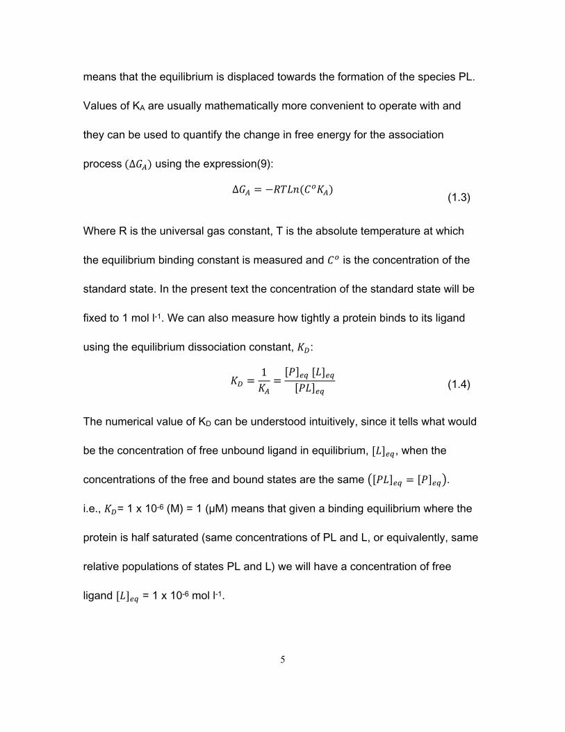
means that the equilibrium is displaced towards the formation of the species PL.
Values of KA are usually mathematically more convenient to operate with and
they can be used to quantify the change in free energy for the association
process ∆ using the expression(9):
∆(1.3)
Where R is the universal gas constant, T is the absolute temperature at which
the equilibrium binding constant is measured and is the concentration of the
standard state. In the present text the concentration of the standard state will be
fixed to 1 mol l-1. We can also measure how tightly a protein binds to its ligand
using the equilibrium dissociation constant, :
1 (1.4)
The numerical value of KD can be understood intuitively, since it tells what would
be the concentration of free unbound ligand in equilibrium, , when the
concentrations of the free and bound states are the same .
i.e., = 1 x 10⁻⁶ (M) = 1 (µM) means that given a binding equilibrium where the
protein is half saturated (same concentrations of PL and L, or equivalently, same
relative populations of states PL and L) we will have a concentration of free
ligand = 1 x 10⁻⁶ mol l-1.

6
The relative populations of the bound ( ) and free ( ) states of the protein are
given by:
; (1.5)
From equation (1.6) we can shown that 1 . Both populations, and
have a range of [0,1] . 0 or equivalent to 1 meaning fully free
unbound protein; and 1 or equivalent to 0 meaning fully saturated or
completely bound protein.
1.3. Binding equilibrium constants in a system exchanging between two states
Measuring protein ligand binding equilibrium constants is possible through the
use of different experimental tools. In most of the cases a mathematical model
must be defined first, and then subsequent data analysis is required to extract
KA. Fortunately, for most of all the experimental techniques the model shares the
same mathematical structure.
Suppose we have an experimentally measured variable called that is a linear
function of the relative populations at equilibrium of the protein in the free and
bound states , .
This variable can be expressed for any values of and as:
, 1 (1.6)
7
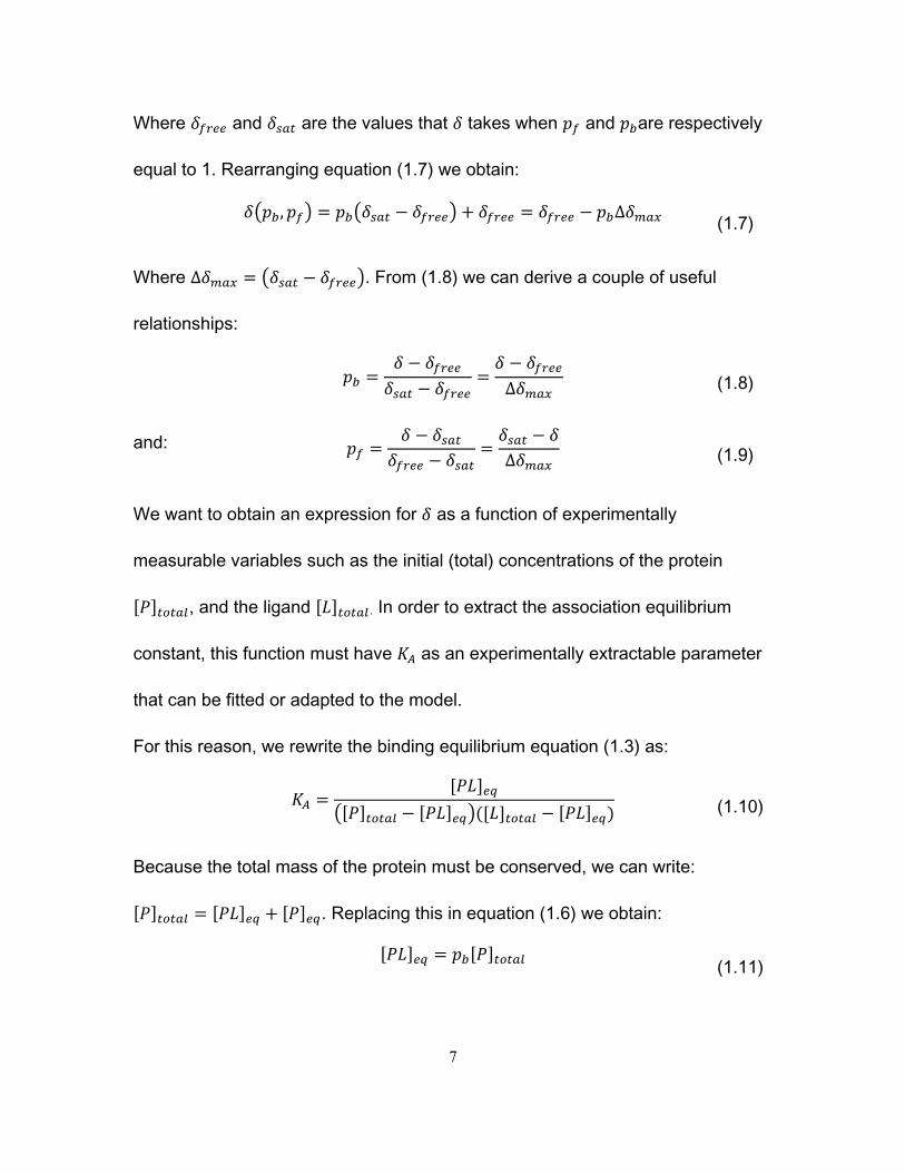
Where and are the values that takes when and are respectively
equal to 1. Rearranging equation (1.7) we obtain:
, ∆ (1.7)
Where ∆ . From (1.8) we can derive a couple of useful
relationships:
∆
(1.8)
and: ∆
(1.9)
We want to obtain an expression for as a function of experimentally
measurable variables such as the initial (total) concentrations of the protein
, and the ligand . In order to extract the association equilibrium
constant, this function must have as an experimentally extractable parameter
that can be fitted or adapted to the model.
For this reason, we rewrite the binding equilibrium equation (1.3) as:
(1.10)
Because the total mass of the protein must be conserved, we can write:
. Replacing this in equation (1.6) we obtain:
(1.11)

8
Replacing (1.12) into (1.11) gives:
/1
(1.12)
Where R is the ratio / .
Expanding and rearranging equation (1.12) gives:
1 1 (1.13)
Which can be expressed as a quadratic expression of :
11
0 (1.14)
The real root of this equation is:
√ 42
(1.15)
Where 1 . Replacing the value of from equation (1.8) in
equation (1.15) gives (10):
∆2
4 (1.16)
Equation (1.16) represents the variable as a function of and as
we wanted. It also has the affinity binding constant as a fitting parameter. This
equation is a basic tool for the analysis of any titration curve in a system
exchanging between two states described in equation (1.1).
can be measured using several physical techniques. It is desirable that the
selected property to be measured changes linearly with the extent of the

9
association process. This will make easier the fitting procedure that is used to
measure the affinity binding constant .
potentially can be intrinsic fluorescence intensity of the protein or the ligand.
For some other systems can be the frequency associated with a magnetic
resonance signal coming from nuclear spins present in the protein or the ligand.
In all the previous scenarios our function will provide a tool to quantify the
association equilibrium constant .
The final goal of studying protein ligand binding thermodynamics is to understand
how the binding landscape is modulated by changes in free energy, entropy and
enthalpy upon binding. This approach can be used to identify the main driving
forces behind the association process and in some cases can provide
underpinning molecular information relative to binding. However, studying
thermodynamics of binding alone will provide just a "static picture" of the relative
stabilities between the free and bound states. In this way we will obtain valuable
quantitative information on the change in thermodynamic variables upon binding.
However, any information about intermediate states, or transition states that exist
between the free species and the final bound complex are therefore invisible.
Any stability or molecular changes in those intermediate states are essentially
unknown. In theory, an infinite number of energy pathways can similarly explain
10
the changes in thermodynamic variables between the free unassociated species
and the final bound protein-ligand complex(11).
If we want to gain more information about the intermediate states during protein-
ligand binding it is essential to measure dynamics (or kinetics) of the association
process. Some experimental techniques, such as Nuclear Magnetic Resonance
(30) can provide detailed atomic resolution information on intermediate states
during protein-ligand association(12). Without the use of NMR some of these
intermediate states would be virtually undetectable or "invisible".
Following the analogy that describes protein-ligand binding thermodynamics as a
tool that provides a "static picture" of the relative stabilities of the free and bound
states, we can take the analogy one step further saying that the study of protein-
ligand binding kinetics will deliver an extra and helpful "snapshot" of the relative
stability of any intermediate binding state.
1.4. Protein-ligand dynamics
There is an additional and perhaps complementary view to understand the
binding equilibrium reaction described in equation (1.1). This approach implies
that any binding equilibrium is dynamic. The measured macroscopic value of any
equilibrium constant is merely a consequence of the principle of detailed
balance(13). This principle states that for a complex reaction in equilibrium the
11
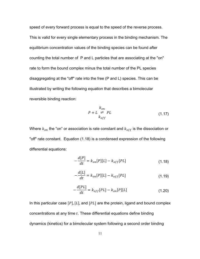
speed of every forward process is equal to the speed of the reverse process.
This is valid for every single elementary process in the binding mechanism. The
equilibrium concentration values of the binding species can be found after
counting the total number of P and L particles that are associating at the "on"
rate to form the bound complex minus the total number of the PL species
disaggregating at the "off" rate into the free (P and L) species. This can be
illustrated by writing the following equation that describes a bimolecular
reversible binding reaction:
⇌ (1.17)
Where the “on” or association is rate constant and is the dissociation or
"off" rate constant. Equation (1.18) is a condensed expression of the following
differential equations:
(1.18)
(1.19)
(1.20)
In this particular case , , and are the protein, ligand and bound complex
concentrations at any time . These differential equations define binding
dynamics (kinetics) for a bimolecular system following a second order binding
12
reaction. , , and are not limited to equilibrium values anymore. In fact,
at equilibrium, all the time derivatives of the concentrations are zero, and
equations (1.19), (1.20) and (1.21) are equivalent to equation (1.3).
From this is clear that:
1 (1.21)
Equations (1.19) through (1.21) describe a simple one step reversible
bimolecular binding reaction formerly introduced in equation (1.1).
If we define the following boundary conditions: At 0, , and
; At , , and ,
where is either the increase in the concentration of the species PL at an
arbitrary time compared to , or the decrease in the concentration of the
species P and L at time t compared to the respectively initial values and
.
We can now write the following differential equation:
(1.22)
After expanding we obtain:
(1.23)
If we define: ; ;
. We can write equation (1.24) as:

13
(1.24)
A solution for this differential equation is:
/2
/2 (1.25)
Where: 4 ; / .
We can also find a more simple and experimental useful solution defining the
following boundary conditions: 0, , 0;
Equation (1.26) can be written now as (14):
2 1
2 1 (1.26)
Where 1 4 / and , is a
constant.
Equations (1.26) or (1.27) are some of the fitting tools that we can use to
measure the dissociation ( ) rate constant and the dissociation rate constant
( for a bimolecular reversible binding system. They will also provide a value
for the equilibrium constant . The only requirement to do so, is to select
a physical measurable property that can be a linear function of the values of ,
or between the free and the equilibrium state.
14
We will use again the function to track the association process, but in this case
will be also a function of time. We need to define a time dependent function
such as:
(1.27)
Where: = , , and are the values
that takes respectively at the free unbound state and at the fully saturated
bound system.
Under these conditions we can write equation (1.28) as:
(1.28)
(1.29)
Equation (1.30) makes a variable that only depends of time. In some cases
can be fluorescence, optical absorbance, circular dichroism, infrared,
electron paramagnetic resonance or light scattering, measured as a function of
time during protein-ligand binding. In order to be experimentally useful, must
be well defined and measurable at the free unbound state and at the
thermodynamic equilibrium.
Measuring binding kinetics using the previous approach requires the rapid mixing
of free protein and free ligand. Then, during the association time the formation of
15
the bound complex is followed or measured using an appropriate physical
variable . The system obviously starts far from thermodynamic equilibrium.
Under these circumstances binding kinetics becomes a study case of mass
transport phenomena coupled to a collision-docking event. This means that the
protein-ligand binding process can be separated into two fundamental steps:
First, diffusion of protein and ligand in a concentration gradient towards their
binding partners(15); and second, a collision-docking event that requires either
the right orientation and the proper kinetic energy in order to make this final step
a binding event(16).
Studying protein-ligand binding dynamics through mixing techniques requires
that the time of mixing of the reagents must be faster than the time that the
association process takes place, otherwise the measure of protein ligand binding
kinetics is not feasible. There is a maximum upper limit for the binding
association rate(17). This theoretical limit considers a diffusion-controlled
reaction. In this theoretical binding scheme every single collision between the
protein and ligand will form a final bound complex. This upper limit describing
binding at the diffusion limit can be mathematically calculated after defining
certain conditions in the system(15).
16
1.5. Protein ligand binding limited by diffusion
We will consider again the reversible bimolecular binding reaction ⇌ . It
will be assumed that protein (P) and ligand (L) are spherical uncharged
molecules without any potential energy of interaction between them. We want to
calculate an expression for the rate at which P and L collide. Under these
conditions, we will obtain an expression for the bimolecular rate constant for a
system binding at the diffusion limit. In a first instance we can assume that P is
an immobile protein molecule, and that molecules of L diffuse into P colliding with
it to form the bound complex PL(14). Using first Fick´s law we can write an
expression to calculate the rate of flow of L molecules per unit area in the space
(Flux, ) as:
(1.30)
Where is the diffusion coefficient for the ligand in the solution and is the
ligand concentration in molecules per volume unit.
It will be assumed that the concentration of L only changes with the distance r
measured from the center of mass of every protein. For this reason we can set
the following conditions using spherical coordinates: 0 and 0.
Now Fick's equation becomes:
∂∂r
(1.31)
17
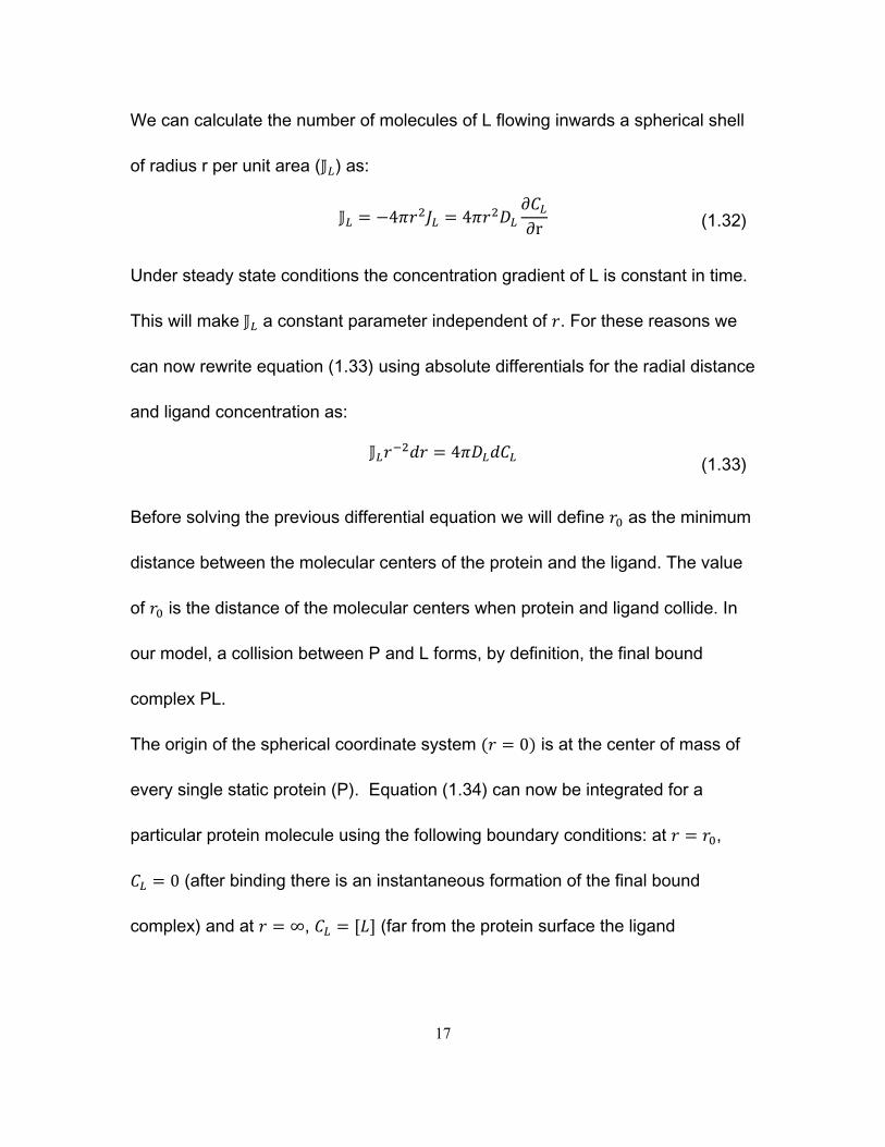
We can calculate the number of molecules of L flowing inwards a spherical shell
of radius r per unit area ( ) as:
4 4∂∂r
(1.32)
Under steady state conditions the concentration gradient of L is constant in time.
This will make a constant parameter independent of . For these reasons we
can now rewrite equation (1.33) using absolute differentials for the radial distance
and ligand concentration as:
4(1.33)
Before solving the previous differential equation we will define as the minimum
distance between the molecular centers of the protein and the ligand. The value
of is the distance of the molecular centers when protein and ligand collide. In
our model, a collision between P and L forms, by definition, the final bound
complex PL.
The origin of the spherical coordinate system 0 is at the center of mass of
every single static protein (P). Equation (1.34) can now be integrated for a
particular protein molecule using the following boundary conditions: at ,
0 (after binding there is an instantaneous formation of the final bound
complex) and at ∞, (far from the protein surface the ligand
18
concentration is constant and is equal to the ligand's concentration in the bulk
solution ).
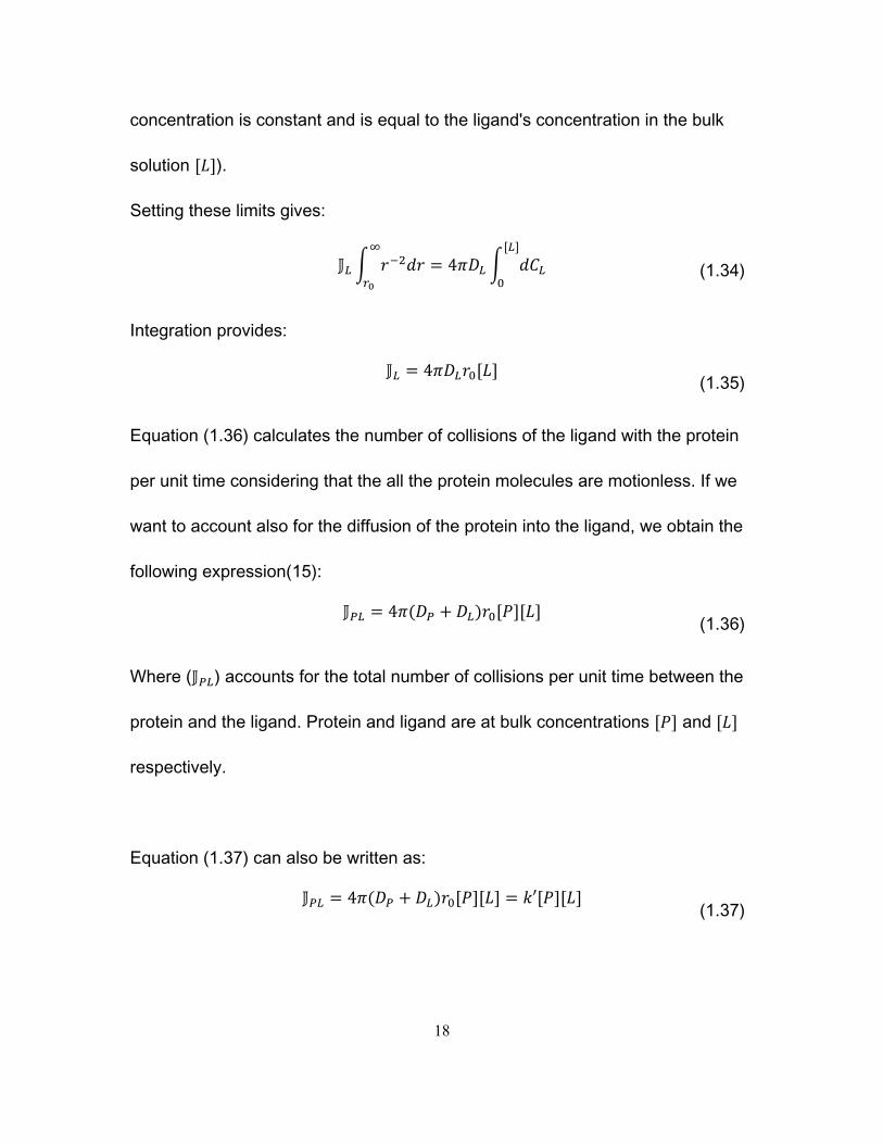
Setting these limits gives:
4 (1.34)
Integration provides:
4(1.35)
Equation (1.36) calculates the number of collisions of the ligand with the protein
per unit time considering that the all the protein molecules are motionless. If we
want to account also for the diffusion of the protein into the ligand, we obtain the
following expression(15):
4(1.36)
Where ( ) accounts for the total number of collisions per unit time between the
protein and the ligand. Protein and ligand are at bulk concentrations and
respectively.
Equation (1.37) can also be written as:
4 ′(1.37)
19
Where 4 . Using Avogadro´s number ( , we can use the
value of to finally calculate the bimolecular association rate constant for
protein-ligand binding, , as:
4(1.38)
Expression (1.38) sets a theoretical limit for the maximum speed of the
association rate under the conditions previously defined. There are systems that
show even higher association binding rates than those derived for a diffusion-
controlled binding reaction. This is the case for a protein and ligand binding
under the effect of an attractive electrostatic potential. An example of such a
system will be illustrated in chapter 3.
Systems binding close to diffusion limit are considered fast binders.
Measurement of fast binding kinetics in protein-ligand binding is a challenging
experimental task. In most of the cases, mixing methods used to measure
dynamics are not suitable to measure fast binding kinetics(14). In these cases,
other techniques, such as relaxation methods, are recommended. The principle
behind relaxation techniques is to start with a protein-ligand system at
equilibrium. A pulse signal (temperature, pressure, radiation) is suddenly applied
displacing the system towards a new equilibrium. The speed at which the pulse is
applied must be much faster that the time that takes to the system to move or
"relax" to the new equilibrium. The time that the system takes to arrive at the new
20
equilibrium is measured (relaxation time). This is done following over the time a
physical variable that measures the change in concentration of the binding
species through the transition between equilibria. The interesting part of the
relaxation methods is that the shape of the curve that tracks the changes on
concentration also encodes the values of the on and off rates of the system.
In our particular case, when the association process is in the millisecond to
microsecond time scale, certain NMR relaxation dispersion techniques can be
used to measure protein binding kinetics. We will have a look to these and other
techniques in chapter 2.
At this point we have considered that every single collision between the protein
and ligand leads to the formation of the final bound complex (PL). This is not the
general rule and it is only true in a very few exceptional cases in biological
systems(18). A more realistic picture to describe a true collision between protein
and ligand can be illustrated in the following paragraphs.
We can have two types of collisions in bimolecular protein ligand binding. In one
of them protein and ligand collide to form an unproductive protein-ligand
encounter complex. In this case, after the collision, the protein and ligand
dissociate. In a second type of protein-ligand encounter pair, protein and ligand
have the right geometrical orientation and favorable kinetic energy. This will
make this protein-ligand collision a productive encounter complex. A productive
21
encounter complex will have the highest probability to evolve towards the
formation of the final bound state. This type of favorable binding collisions or
productive complexes are sometimes indistinctively named as the "encounter
complex"(19), the "encounter pair"(20), the "activated complex"(21) or the
"transition state"(22). We will use the term transition state to describe this type of
productive collisions in the remaining part of this document.
1.6. Association rate constants and transition state
As explained previously, protein ligand association process can be studied as a
diffusion step coupled to a docking event. If the docking event is faster than the
diffusion step, is a direct measure of the number of productive collisions
between ligand and protein. The binding process in this case is said to be
diffusion controlled(16).
If the formation of the stereo-specific complex is slower than the diffusion rate,
the association process is governed by this particular "activated" step and the
kinetics of binding is said to be under activation control(18). How do we know if a
particular binding process is diffusion controlled or otherwise an activated one?
What is the meaning of in both binding processes?
In order to answer the second question we will use an approach where chemical
kinetics will be considered as a valid approximation to describe kinetics of protein
22
ligand biding. We can start by looking again to equation (1.22): . This
expression sets a bridge between dynamics and thermodynamics of bimolecular
reversible binding processes. Taking the temperature derivative of the natural
logarithm on both sides of equation (1.22) gives:
(1.39)
Left-hand side of equation (1.40) can be expressed using Van't Hoff's equation:
∆ (1.40)
We can now rewrite equation (1.40) as:
∆ (1.41)
Van't Hoff was the first person to hint that both terms in the right-hand term of
equation (1.41) could be expressed in the form (18,23):
(1.42)
However, it was Svante Arrhenius who proposed for the first time a molecular
model to explain association and dissociation rate constants. He suggested that
certain reactant molecules (in our case P and L binding species) must be in an
"activated state" that lead them to form the final product (final bound state in our
case). These "active" molecules must be also in equilibrium with the rest of the
23
reactant molecules and the rate constant must be proportional to the difference in
energy between the active to normal reactant molecules(24).
If we apply Van't Hoff's equation to the equilibrium described by Arrhenius i.e.,
the equilibrium between active and regular reactant molecules, we obtain:
∆ ‡
(1.43)
Where ∆ ‡ denotes the change in enthalpy between the active molecules and
the normal reactant molecules. ∆ ‡ is in this way defined as the activation
energy for the reaction process. In our case ∆ ‡ is the activation energy for the
protein-ligand association process.
We can finally write a more familiar equation for after integrating equation
(1.44):
∆ ‡
(1.44)
Where constant A is an integration constant.
In chapter 3 it will be illustrated how ionic strength can modulate "on" rates in
protein-ligand binding driven by electrostatic interactions. The relationship
between electrostatics and association rate constants can provide insights about
the molecular structure of the transition state. This will be illustrated in a protein-
ligand system that binds under diffusion control. Chapter 4 will show the effect of
pressure in the association rate constant for a bimolecular reversible binding
24
system. Analysis of kon as a function of pressure provided information about the
relative change in volume of the transition state. This value can be correlated to
changes in solvation of the system through binding.
The additional question remaining to be answered consists in finding a way to
identify when a bimolecular reversible binding process is controlled by diffusion.
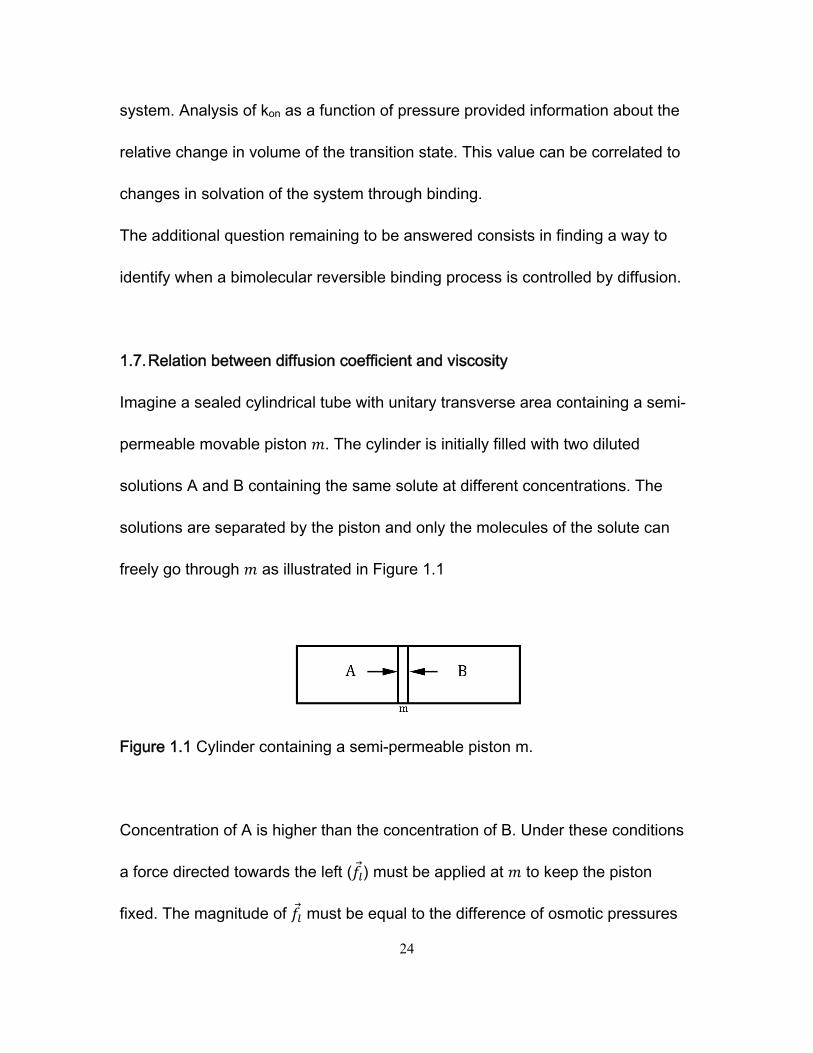
1.7. Relation between diffusion coefficient and viscosity
Imagine a sealed cylindrical tube with unitary transverse area containing a semi-
permeable movable piston . The cylinder is initially filled with two diluted
solutions A and B containing the same solute at different concentrations. The
solutions are separated by the piston and only the molecules of the solute can
freely go through as illustrated in Figure 1.1
Figure 1.1 Cylinder containing a semi-permeable piston m.
Concentration of A is higher than the concentration of B. Under these conditions
a force directed towards the left ( ) must be applied at to keep the piston
fixed. The magnitude of must be equal to the difference of osmotic pressures
25
times the transverse area. For sake of simplicity the transversal surface will have
an area of value 1 for a given arbitrary area units. If is removed, the piston will
displace towards the right to achieve a final equilibrium. At equilibrium, the solute
concentration at both sides of must the same. Therefore, diffusion driven by
osmotic pressure will match solute concentration at both sides of . This
experiment shows that osmotic pressure can be seen as the driving force in
diffusion processes(25).
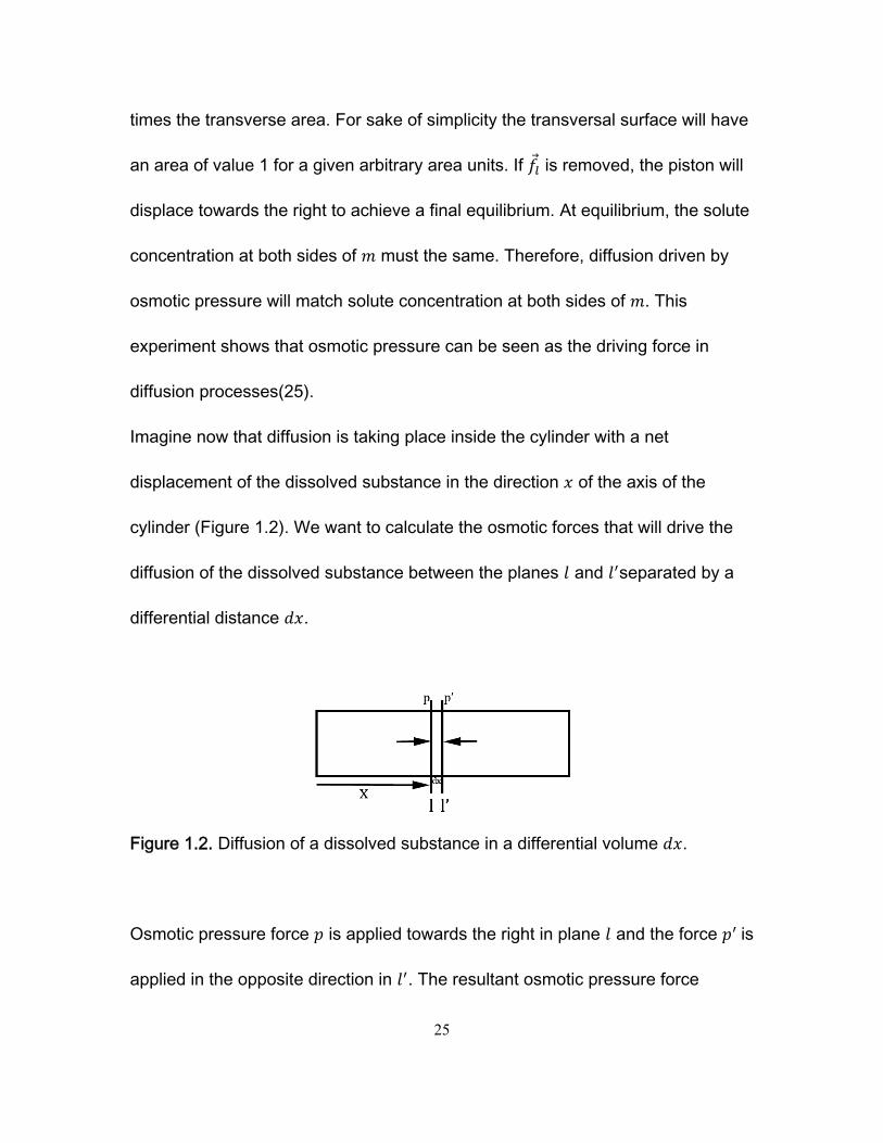
Imagine now that diffusion is taking place inside the cylinder with a net
displacement of the dissolved substance in the direction of the axis of the
cylinder (Figure 1.2). We want to calculate the osmotic forces that will drive the
diffusion of the dissolved substance between the planes and separated by a
differential distance .
Figure 1.2. Diffusion of a dissolved substance in a differential volume .
Osmotic pressure force is applied towards the right in plane and the force is
applied in the opposite direction in . The resultant osmotic pressure force

26
applied over the differential volume segment is: . If we want to calculate
the volumetric osmotic pressure (K), i.e. the osmotic pressure force that acts in
the dissolved substance contained between and per unit volume, we obtain:
(1.45)
Any diluted solute is known to exert an osmotic pressure over the solvent that
follows Van't Hoff's equation(26):
(1.46)
Where the molar concentration of the dissolved particle, R is is the gas
constant and T is the absolute temperature of the system. Because the diffusion
process is proceeding on the x direction is obvious that the concentration of the
dissolved particle is a function of . From equation (1.16) and (1.47) we can
write:
(1.47)
Now we need to calculate the kinetic force necessary to move a particle that is
diffusing at a speed through the planes and . Calculation of involves the
solution of differential equations (Navier-Stokes equations) that cannot be
integrated for a general case. However, we can define certain boundary
conditions close to experimental circumstances that will make Navier-Stokes
equation soluble. The boundary conditions assume a spherical diffusing particle
27
with a much bigger diameter than the solvent particles. Also, the speed at which
the sphere moves through the solution, , must be very slow i.e. "Stokes flow".
This means that the diffusing particle must move at a speed slow enough to
cause a laminar flow (low Reynolds number condition) between the moving
sphere and the surrounding solvent. Under these conditions we can calculate the
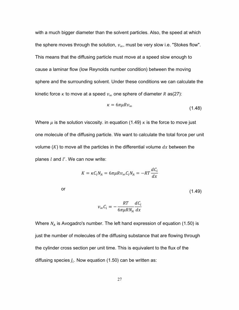
kinetic force to move at a speed one sphere of diameter as(27):
6(1.48)
Where is the solution viscosity. in equation (1.49) is the force to move just
one molecule of the diffusing particle. We want to calculate the total force per unit
volume ( ) to move all the particles in the differential volume between the
planes and . We can now write:
6
or
6
(1.49)
Where is Avogadro's number. The left hand expression of equation (1.50) is
just the number of molecules of the diffusing substance that are flowing through
the cylinder cross section per unit time. This is equivalent to the flux of the
diffusing species . Now equation (1.50) can be written as:
28
6
(1.50)
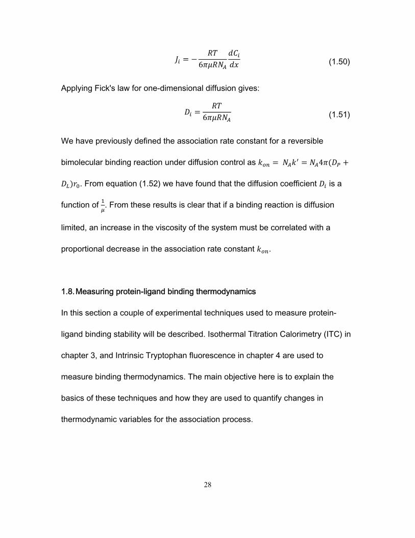
Applying Fick's law for one-dimensional diffusion gives:
6
(1.51)
We have previously defined the association rate constant for a reversible
bimolecular binding reaction under diffusion control as 4
. From equation (1.52) we have found that the diffusion coefficient is a
function of . From these results is clear that if a binding reaction is diffusion
limited, an increase in the viscosity of the system must be correlated with a
proportional decrease in the association rate constant .
1.8. Measuring protein-ligand binding thermodynamics
In this section a couple of experimental techniques used to measure protein-
ligand binding stability will be described. Isothermal Titration Calorimetry (ITC) in
chapter 3, and Intrinsic Tryptophan fluorescence in chapter 4 are used to
measure binding thermodynamics. The main objective here is to explain the
basics of these techniques and how they are used to quantify changes in
thermodynamic variables for the association process.
29
1.8.1. Isothermal Titration Calorimetry, model for 1:1 binding
Isothermal Titration Calorimetry (ITC) is a method used to gain thermodynamic
information of chemical reactions or binding processes(28). We will describe the
use of this technique to measure protein-ligand binding thermodynamics. A
typical ITC apparatus consists of a small reaction cell. In the reaction cell one of
the unbound binding partners is initially confined. The free binding counterpart is
loaded in a syringe. During the experiment the sample in the syringe is injected
stepwise into the reaction cell.
For sake of simplicity assume that free unbound protein is initially loaded in the
reaction cell and the free ligand is loaded in the syringe. During the titration, the
ligand is isothermically injected and mixed in n steps into the reaction cell. After
every injection, the reaction cell achieves eventually a new thermodynamic
equilibrium at constant temperature. Before the th injection, the reaction cell will
contain an equilibrium solution with a total ligand to protein concentration ratio
,
,. Where , and , are respectively the total ligand and protein
concentration. Through stepwise injections of the ligand into the reaction cell,
different concentrations ratios ,
, are obtained, and therefore different
populations of the final bound state are sampled. The experiment is usually
designed to start with injections that will provide solutions at equilibrium where
the bound state (PL) is more populated, and the titration will likely finish with
30
injections where the equilibrium solution in the cell is almost completely displaced
towards the unligated state (P+L). The instrumental setup in a calorimeter
measures the power required to maintain the reaction cell at the desired
experimental temperature. This power is compared with the power dissipated as
heat in a reference cell that is also kept at the same experimental temperature.
The difference between these powers, also called differential power is followed
and recorded during the time and it is used to measure the amount of heat
released or absorbed after every single ligand injection. By doing so, the
experiment provides a titration curve where values of are plotted as a function
of the ligand to protein concentration ratio.
If the amount of heat released at each injection is only due to protein ligand
binding, the value of in the th injection will be proportional to the net formation
of the final PL complex in the reaction cell volume . At each injection, ITC
apparati are usually designed to displace an equal volume from the reaction
cell. Under these conditions we can calculate the total concentration of the
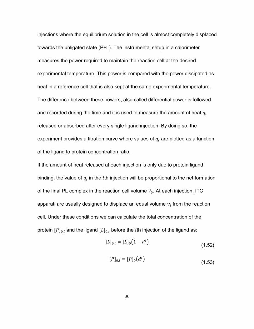
protein , and the ligand , before the th injection of the ligand as:
, 1 (1.52)
, (1.53)
31
Where 1 is the dilution factor, is the ligand concentration in the
syringe and is the initial protein concentration in the reaction cell. For every
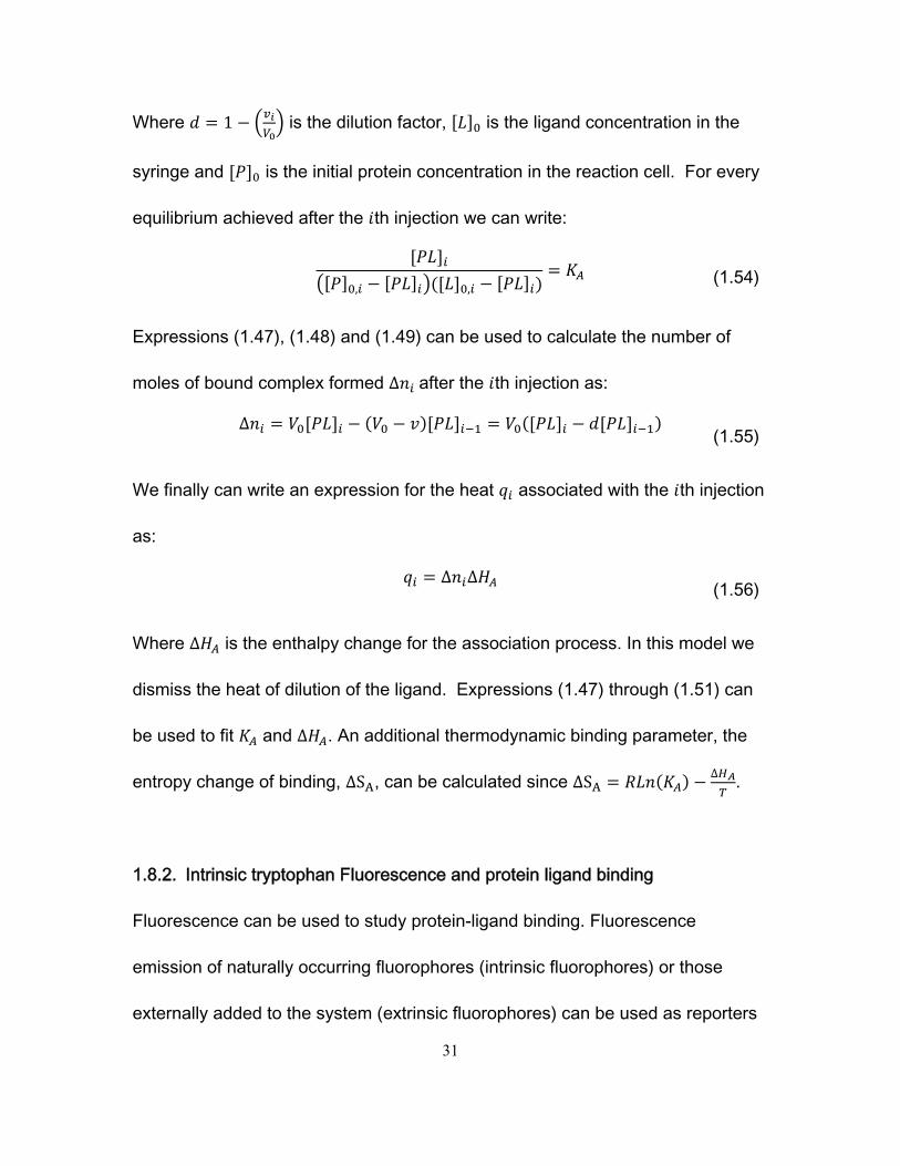
equilibrium achieved after the th injection we can write:
, ,
(1.54)
Expressions (1.47), (1.48) and (1.49) can be used to calculate the number of
moles of bound complex formed ∆ after the th injection as:
∆ (1.55)
We finally can write an expression for the heat associated with the th injection
as:
∆ ∆(1.56)
Where ∆ is the enthalpy change for the association process. In this model we
dismiss the heat of dilution of the ligand. Expressions (1.47) through (1.51) can
be used to fit and ∆ . An additional thermodynamic binding parameter, the
entropy change of binding, ∆S , can be calculated since ∆S ∆ .
1.8.2. Intrinsic tryptophan Fluorescence and protein ligand binding
Fluorescence can be used to study protein-ligand binding. Fluorescence
emission of naturally occurring fluorophores (intrinsic fluorophores) or those
externally added to the system (extrinsic fluorophores) can be used as reporters
32
to study dynamics and thermodynamics of binding in several biological
phenomena. The most significant intrinsic fluorophore in proteins is the indole
group of tryptophan. Intrinsic tryptophan fluorescence can be used to study
dynamics and thermodynamics of biding as explained in sections (1.2) and (1.3).
Centre of mass for the fluorescence emission spectra and fluorescence intensity
are two properties that can be used to study dynamics and thermodynamics of
binding. More details about these measurement techniques can be seen in
chapter 4.
A protein's intrinsic tryptophan fluorescence depends on the polarity of the
solvent in which this fluorophore is dissolved. The indole group in tryptophan can
show a displacement in the maximum fluorescence emission spectrum according
the solvent used (Stokes shift(29)). The stokes shift can be also useful in order to
understand structural changes in the protein during the association process.
Tryptophan fluorescence intensity may show Stokes shifts towards lower
wavelengths when indole group changes from a polar solvent accessible
environment towards a non-polar one. This can be used to understand protein
conformational changes upon ligand binding(30). The same principle can be
used to gain information about the structure and stability of the transition state.
Chapter 3 makes extensive use of NMR dispersion relaxation experiments
together with intrinsic tryptophan fluorescence measurements to study dynamics
33
and thermodynamics of protein ligand binding. Kinetics and thermodynamics of
binding are used to map volume changes in protein-ligand association
processes.
1.9. Biological systems
Experimental results described in chapters 3 through chapter 5 were obtained
using several protein-ligand complexes. These biological systems were selected
to study dynamics and thermodynamics of binding. The protein used in the first
case is the chicken isoform of Src Homology 3 (SH3) binding domain of the
tyrosine kinase FYN(31). Chapters 3 and 4 used recombinant protein FYN SH3
domain that binds to a series of dodecapeptides containing a proline rich motif.
This short proline motif is recognized by the SH3 domain as a canonical binding
sequence.
Chapter 5 briefly describes some techniques used to obtain special patterns of
isotopic labeling of human Farnesyl Pyrphosphate Synthase (hFPPS)(32).
Isotopically labeled 1H-15N hFPPS was initially expressed and purified to study
binding of the protein with bisphosphonates and allosteric inhibitors. However,
bidimensional NMR spectra lacked of enough signal resolution to perform these
studies. Special isotopic labeling techniques were used aiming to improve NMR
spectral quality. Different isotopic labeled versions of hFPPS were successfully
34
expressed and purified. These proteins were nevertheless not suitable to perform
NMR experiments to study binding of hFPPS with inhibitors.
1.9.1. Protein interaction domains
Many protein-protein interactions are mediated in nature by modular interaction
domains(33). These domains are also important in protein interactions with other
biomolecules including DNA, RNA and membrane lipids. Interaction domains are
usually 30 to 200 amino acids size proteins that can share similar structural and
binding characteristics. They modulate several biological functions including cell
growth, polarity, motility, differentiation and signaling. There is a group of
interaction domains that recognize proline as a binding target. This domains are
called proline recognition domains (PRD's)(34).
A special group of PRD's consist in small ~60 amino acid interaction modules
named Src Homology 3 (SH3) domains(35). These domains are ubiquitous in
eukaryotes and accomplish a wide variety of functions in signaling processes
inside the cell. SH3 domains have evolved to bind to a many different ligands.
This binding promiscuity explains in part the implication of SH3 domains in
numerous cellular processes. Most of SH3 domains bind to a proline rich motif
consisting of the sequence PxxP, where P is proline and x is any amino acid.
Proline rich sequences usually binds to SH3 domains in two canonical ways:
35
+xΦPxΦP or type I, and ΦPxΦPx+ or type II. Where + is a positively charged
residue, x is any amino acid, Φ is a hydrophobic residue and P is proline.
Both types of proline rich motifs adopt a helical conformational structure called
polyproline II (PPII)(36). This is a left-handed helix that is not only recognized by
SH3 domains but by all the PRD's(37).
1.9.2. Proline rich motifs and polyproline II conformation
Any amino acid involved in protein binding must be preferentially located in the
solvent exposed surface of the protein(37). This makes it more accessible to the
binding counterpart. From all the naturally occurring amino acids proline is
perhaps the most suitable residue to accomplish this function(38). Proline usually
breaks secondary structures such as -helices and -sheets(39). These
disrupting points are usually exposed to solvent(38). For this reason proline is
more likely found on the surface of the protein and less likely found at internal
buried residues(38). Furthermore, proline forms a five ring heterocycle between
the side chain and its backbone. This restricts the dihedral angle Φ for this
residue to an approximate value of -60⁰ which reduces the number of
conformations that proline rich peptides can tolerate. The most probable
conformation that two or more sequential prolines can adopt consists of
polyproline II (PPII). This left handed helix has 3 residues per turn with a
36
conformation less rigid than an ideal alpha helix. An ideal alpha helix has an
average pitch of 3.6 residues. PPII conformation occurs naturally when certain
number of proline residues are present in a given polypeptide sequence.
Formation of PPII helices by free-unbound proline rich motifs seems to reduce
the entropy penalty of any binding domain that interacts with these
sequences(37). PPII has sidechains and carbonyl groups pointing towards
outside the helix, making them more exposed to interact with binding
counterparts. Additionally, the lack of an amide proton in proline hinders intra-
molecular hydrogen bonds with carbonyl group in a PPII conformation. This gives
more freedom to carbonyl groups to interact with binding sites. Changes in the
constituent residues in a proline rich region usually preserve the PPII
conformation. This is the reason why so many different combinations of proline
and non-proline residues form PPII structures. This explains the relative
promiscuity of PRD's and the flexibility that SH3 domains show to mediate in
binding in so many different cellular signaling processes(40).
1.9.3. Fyn SH3
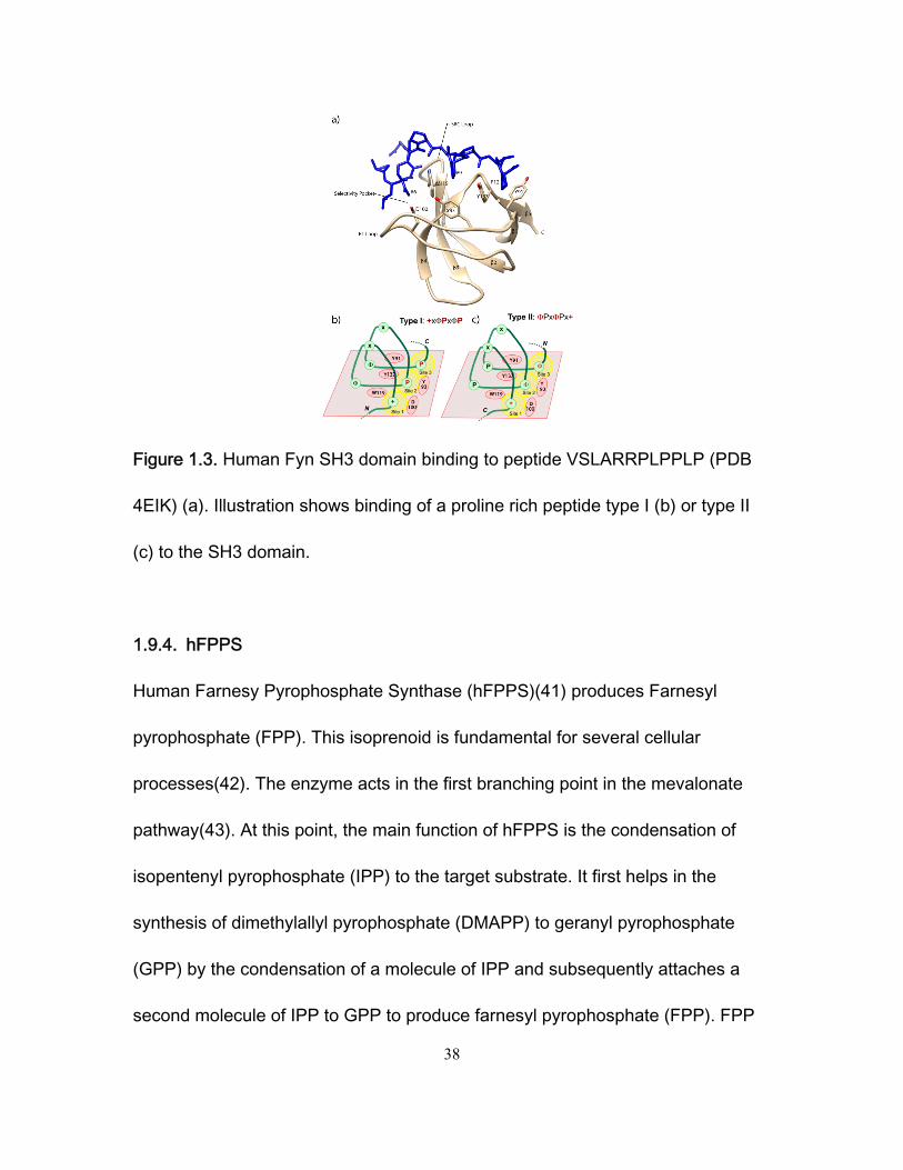
The Fyn SH3 domain is illustrated in Figure 1.3. It shows a human Fyn SH3
domain binding to a proline rich motive type II: VSLARRPLPPLP (PDB 4EIK).
Fyn SH3 domains display a typical beta barrel structure with five anti-parallel
37
beta sheets and several loops. The most significant ones are the n-src loop and
the RT loop. The latter is a disordered region that contains a conserved RT
amino acid sequence. Fyn associates with type I (+xΦPxΦP) and type II
(ΦPxΦPx+) proline rich motives using three binding pockets. Site 1 (Figs. 1.3b,
1.3c) is a selectivity pocket that receives a positively charged residue located at
the canonical site (+) in the ligand peptide. Residue (+) forms an ion pair with a
negatively charged residue in the binding pocket (D or E). Electrostatic
interactions of the charged residue (+) are usually enhanced by long distance
electrostatic interactions. These are due to the presence of additional negatively
charged residues close to the specificity pocket. Site 2 and site 3 (Figs 1.3b,
1.3c) can either dock consensus proline residues or consensus hydrophobic
residues when respectively binds proline rich peptides type I (Fig. 1.3b) or type II
(Fig. 1.3c). Experimental results shown in chapter 3 also confirm that proline rich
peptides lacking the consensus residue (+) can also bind to the FYN SH3 binding
domain. This is a proof that the absence of electrostatics interactions usually
present in the selectivity pocket when Fyn binds to proline rich peptides, does not
hamper ligand recognition by Fyn.
38
Figure 1.3. Human Fyn SH3 domain binding to peptide VSLARRPLPPLP (PDB
4EIK) (a). Illustration shows binding of a proline rich peptide type I (b) or type II
(c) to the SH3 domain.
1.9.4. hFPPS
Human Farnesy Pyrophosphate Synthase (hFPPS)(41) produces Farnesyl
pyrophosphate (FPP). This isoprenoid is fundamental for several cellular
processes(42). The enzyme acts in the first branching point in the mevalonate
pathway(43). At this point, the main function of hFPPS is the condensation of
isopentenyl pyrophosphate (IPP) to the target substrate. It first helps in the
synthesis of dimethylallyl pyrophosphate (DMAPP) to geranyl pyrophosphate
(GPP) by the condensation of a molecule of IPP and subsequently attaches a
second molecule of IPP to GPP to produce farnesyl pyrophosphate (FPP). FPP
39
is used in the cell to prenylate GTPases that are involved in several cellular
signaling processes. Prenylated GTPases can be then carried out to different
cellular locations(44). Blocking prenylation of GTPases can obstruct several
specific cellular processes (45). For this reason the design of hFPPS inhibitors is
of pharmacological importance. Some inhibitors of hFPSS have been under
clinical use for several years (46). These includes nitrogen containing
bisphophonates (N-BPs)(47). N-BPs have been effectively used in the treatment
of several bone related diseases(48). They are used in treatments where bone
re-absorption is required. Additionally, N-BPs have been used for the treatment
of bone cancer and have also been explored more broadly as general anticancer
agents(49).
N-BPs action on hFPPS has been previously studied through crystallographic
and calorimetric studies (50). N-BPs bind to DMAPP/GPP pocket and mimic the
natural substrates, thus blocking the binding site. This causes a conformational
change that closes the DMAPP/GPP pocket and causes an allosteric
conformational change in the C-tail of the protein(51). This causes a partial
closure of IPP binding site. Further addition of IPP to the system causes a total
closure of IPP pocket and finally locks the protein in an almost irreversible
inactive state.
40
Structural and thermodynamic changes on binding between hFPP and N-BPs
has been previously studied (50). However, there is no information reported
about binding kinetics for this process. One of the main ideas for the system
hFPPs-N-BPs was to apply different NMR techniques in order to understand in
more detail the dynamics of binding. The approach used and the results obtained
are shown in chapter 5.
41
2. Analyzing Protein-Ligand Interactions by Dynamic NMR Spectroscopy
I have coauthored this book chapter with:
Anthony Mittermaier
This book chapter was published in:
Mittermaier, A., and Meneses, E. (2013) Analyzing protein-ligand interactions by dynamic NMR spectroscopy. Methods in molecular biology 1008, 243-266
42
2.1. Summary
Nuclear Magnetic Resonance (NMR) spectroscopy can provide detailed
information on protein-ligand interactions that is inaccessible using other
biophysical techniques. This chapter focuses on NMR-based approaches for
extracting affinity and rate constants for weakly-binding transient protein
complexes with lifetimes of less than about a second. Several pulse sequences
and analytical techniques are discussed, including line-shape simulations, spin-
echo relaxation dispersion methods (CPMG), and magnetization exchange
(EXSY) experiments.
Key words: protein dynamics by NMR spectroscopy, NMR relaxation dispersion
methods, NMR-derived protein-ligand interactions, line-shape analysis of NMR
spectra, protein sample for solution NMR spectroscopy
2.2. Introduction
Solution NMR spectroscopy is a powerful and versatile technique for obtaining
structural and dynamic information on biological molecules and complexes
(52,53). A wide variety of NMR-based approaches can be applied to different
aspects of biological interactions, including the elucidation of the three-
dimensional structures (54-56) and internal motions (57,58) of protein
complexes, the characterization of transiently-populated states in binding
43
pathways (59,60), the rapid screening of small molecule libraries (61,62), and the
determination of the thermodynamic and kinetic parameters of binding. This
chapter focuses on the last application, the determination of biophysical
interaction parameters by NMR.
NMR offers several advantages compared to alternative techniques for
measuring the affinities and timescales of protein interactions. Firstly, NMR
spectra are generally quite sensitive to complex formation, even when
interactions are weak and are not accompanied by large structural
rearrangements (63). Thus NMR is a powerful diagnostic tool for determining
whether two molecules interact. Secondly, simple analyses of the spectral
changes produced by binding rapidly identify those portions of the molecules that
are most involved in the interaction (64,65). Thirdly, NMR can accurately
measure the binding kinetics for transient complexes with extremely short bound
lifetimes of less than 1 ms (66). Such lifetimes are outside the range of most
stopped-flow instruments, because the time required to mix the protein and
ligand solutions is comparable to the time required for the binding reaction to
proceed nearly to completion. Furthermore, NMR kinetics experiments are
performed at equilibrium in solution, which avoids the complication of mass
transport effects that are inherent to surface plasmon resonance measurements
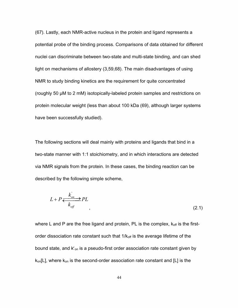
44
(67). Lastly, each NMR-active nucleus in the protein and ligand represents a
potential probe of the binding process. Comparisons of data obtained for different
nuclei can discriminate between two-state and multi-state binding, and can shed
light on mechanisms of allostery (3,59,68). The main disadvantages of using
NMR to study binding kinetics are the requirement for quite concentrated
(roughly 50 μM to 2 mM) isotopically-labeled protein samples and restrictions on
protein molecular weight (less than about 100 kDa (69), although larger systems
have been successfully studied).
The following sections will deal mainly with proteins and ligands that bind in a
two-state manner with 1:1 stoichiometry, and in which interactions are detected
via NMR signals from the protein. In these cases, the binding reaction can be
described by the following simple scheme,
'on
off
kL P PL
k
, (2.1)
where L and P are the free ligand and protein, PL is the complex, koff is the first-
order dissociation rate constant such that 1/koff is the average lifetime of the
bound state, and kon is a pseudo-first order association rate constant given by
kon[L], where kon is the second-order association rate constant and [L] is the
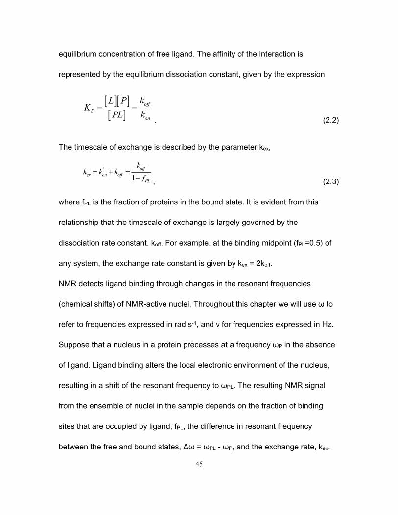
45
equilibrium concentration of free ligand. The affinity of the interaction is
represented by the equilibrium dissociation constant, given by the expression
'
offD
on
kL PK
PL k
. (2.2)
The timescale of exchange is described by the parameter kex,
'
1off
ex on offPL
kk k k
f
, (2.3)
where fPL is the fraction of proteins in the bound state. It is evident from this
relationship that the timescale of exchange is largely governed by the
dissociation rate constant, koff. For example, at the binding midpoint (fPL=0.5) of
any system, the exchange rate constant is given by kex = 2koff.
NMR detects ligand binding through changes in the resonant frequencies
(chemical shifts) of NMR-active nuclei. Throughout this chapter we will use ω to
refer to frequencies expressed in rad s-1, and ν for frequencies expressed in Hz.
Suppose that a nucleus in a protein precesses at a frequency ωP in the absence
of ligand. Ligand binding alters the local electronic environment of the nucleus,
resulting in a shift of the resonant frequency to ωPL. The resulting NMR signal
from the ensemble of nuclei in the sample depends on the fraction of binding
sites that are occupied by ligand, fPL, the difference in resonant frequency
between the free and bound states, Δω = ωPL - ωP, and the exchange rate, kex.
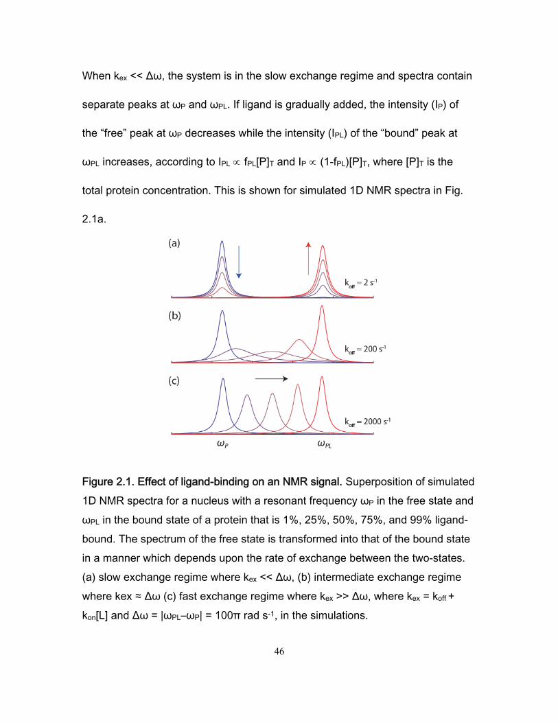
46
When kex << Δω, the system is in the slow exchange regime and spectra contain
separate peaks at ωP and ωPL. If ligand is gradually added, the intensity (IP) of
the “free” peak at ωP decreases while the intensity (IPL) of the “bound” peak at
ωPL increases, according to IPL fPL[P]T and IP (1-fPL)[P]T, where [P]T is the
total protein concentration. This is shown for simulated 1D NMR spectra in Fig.
2.1a.
Figure 2.1. Effect of ligand-binding on an NMR signal. Superposition of simulated 1D NMR spectra for a nucleus with a resonant frequency ωP in the free state and ωPL in the bound state of a protein that is 1%, 25%, 50%, 75%, and 99% ligand-bound. The spectrum of the free state is transformed into that of the bound state in a manner which depends upon the rate of exchange between the two-states. (a) slow exchange regime where kex << Δω, (b) intermediate exchange regime where kex ≈ Δω (c) fast exchange regime where kex >> Δω, where kex = koff + kon[L] and Δω = |ωPL–ωP| = 100π rad s-1, in the simulations.
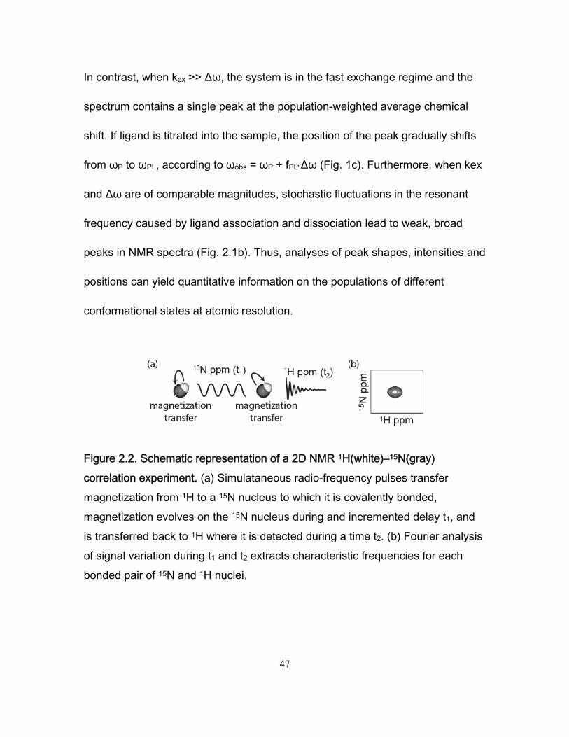
47
In contrast, when kex >> Δω, the system is in the fast exchange regime and the
spectrum contains a single peak at the population-weighted average chemical
shift. If ligand is titrated into the sample, the position of the peak gradually shifts
from ωP to ωPL, according to ωobs = ωP + fPLΔω (Fig. 1c). Furthermore, when kex
and Δω are of comparable magnitudes, stochastic fluctuations in the resonant
frequency caused by ligand association and dissociation lead to weak, broad
peaks in NMR spectra (Fig. 2.1b). Thus, analyses of peak shapes, intensities and
positions can yield quantitative information on the populations of different
conformational states at atomic resolution.
Figure 2.2. Schematic representation of a 2D NMR 1H(white)–15N(gray) correlation experiment. (a) Simulataneous radio-frequency pulses transfer magnetization from 1H to a 15N nucleus to which it is covalently bonded, magnetization evolves on the 15N nucleus during and incremented delay t1, and is transferred back to 1H where it is detected during a time t2. (b) Fourier analysis of signal variation during t1 and t2 extracts characteristic frequencies for each bonded pair of 15N and 1H nuclei.
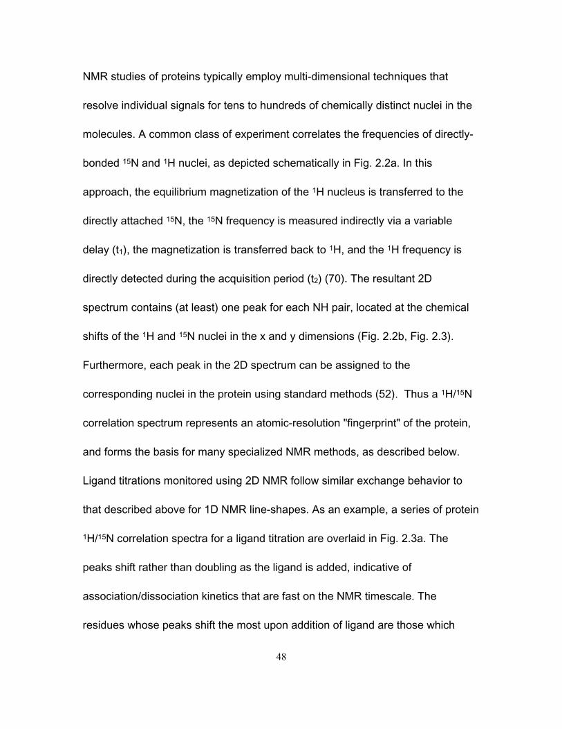
48
NMR studies of proteins typically employ multi-dimensional techniques that
resolve individual signals for tens to hundreds of chemically distinct nuclei in the
molecules. A common class of experiment correlates the frequencies of directly-
bonded 15N and 1H nuclei, as depicted schematically in Fig. 2.2a. In this
approach, the equilibrium magnetization of the 1H nucleus is transferred to the
directly attached 15N, the 15N frequency is measured indirectly via a variable
delay (t1), the magnetization is transferred back to 1H, and the 1H frequency is
directly detected during the acquisition period (t2) (70). The resultant 2D
spectrum contains (at least) one peak for each NH pair, located at the chemical
shifts of the 1H and 15N nuclei in the x and y dimensions (Fig. 2.2b, Fig. 2.3).
Furthermore, each peak in the 2D spectrum can be assigned to the
corresponding nuclei in the protein using standard methods (52). Thus a 1H/15N
correlation spectrum represents an atomic-resolution "fingerprint" of the protein,
and forms the basis for many specialized NMR methods, as described below.
Ligand titrations monitored using 2D NMR follow similar exchange behavior to
that described above for 1D NMR line-shapes. As an example, a series of protein
1H/15N correlation spectra for a ligand titration are overlaid in Fig. 2.3a. The
peaks shift rather than doubling as the ligand is added, indicative of
association/dissociation kinetics that are fast on the NMR timescale. The
residues whose peaks shift the most upon addition of ligand are those which
49
experience the largest changes in local electronic environment due to binding.
For this example, chemical shift displacements are mapped onto the three-
dimensional structure of the protein in Fig. 2.3b. As expected, the largest
changes are observed for residues in the binding site. Chemical shift mapping
approaches, such as this, are a very powerful way to identify protein binding
sites, provided that the structure of the protein is known (64,65).
Direct inspection and quantitative analysis of NMR line-shapes and titration data
can yield information on binding kinetics and affinities, as described in
Subsection 2.3.1. In addition, we will consider two specialized dynamic NMR
techniques that yield even more detailed information, depending on the timescale
of association-dissociation kinetics. In the case of relatively rapid dynamics (kex
values of roughly 10 s-1 to 104 s-1), Carr-Purcell-Meiboom Gill (CPMG) relaxation
dispersion methods can be analyzed to give the populations, interconversion
rates, and chemical shift differences of exchanging states (71) (Subsection
2.3.2). In cases of slower binding kinetics (kex values of roughly 0.5 to 20 s-1)
NMR magnetization exchange (EXSY) experiments (72) quantify the kinetics of
exchange, and help to correlate protein spectra obtained in the free and bound
forms (Subsection 2.3.3).
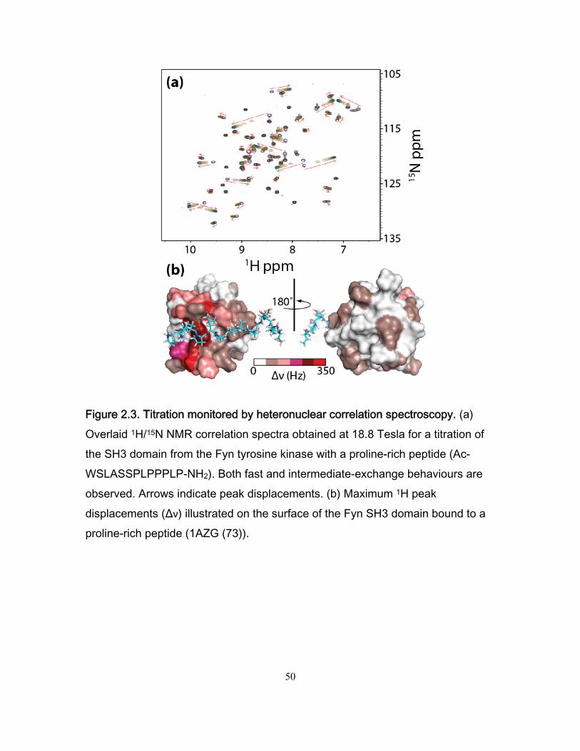
50
Figure 2.3. Titration monitored by heteronuclear correlation spectroscopy. (a) Overlaid 1H/15N NMR correlation spectra obtained at 18.8 Tesla for a titration of the SH3 domain from the Fyn tyrosine kinase with a proline-rich peptide (Ac-WSLASSPLPPPLP-NH2). Both fast and intermediate-exchange behaviours are observed. Arrows indicate peak displacements. (b) Maximum 1H peak displacements (Δν) illustrated on the surface of the Fyn SH3 domain bound to a proline-rich peptide (1AZG (73)).
51
2.3. Materials
2.3.1. NMR samples
In order to study ligand binding using multi-dimensional heteronuclear NMR (as
in Fig. 2.2), protein samples need to be isotopically enriched 15N and/or 13C. In
the case of larger molecules (with molecular weights greater than about 25 kDa),
additional enrichment with 2H can significantly improve spectral quality (74).
Isotopically-labeled protein samples can be over-expressed in bacteria grown in
minimal media containing 15NH4Cl and/or 13C glucose as the sole sources of
nitrogen and/or carbon, respectively (75). Protein samples are typically isolated
with several stages of liquid chromatography that often conclude with size-
exclusion chromatography. Sample purity is of utmost importance, since even
minimal protease contamination can cause extensive protein degradation during
data collection. Protein NMR samples are usually 300 to 600 μL in volume,
contain 5% to 10% D2O (for the spectrometer frequency lock), and are usually
buffered at a pH below 7.5, since base-catalyzed exchange of hydrogen atoms
between protein and solvent can lead to signal loss under more alkaline
conditions (76). Samples can also contain small amounts of EDTA and other
protease inhibitors, as well as NaN3 to prevent microbial contamination. The
minimum protein concentration required for NMR analyses varies, depending on
the spectrometer and particular experiment. In our experience, NMR titrations
52
can be performed with protein concentrations as low as 0.1 to 0.2 mM, using
Varian INOVA spectrometers with field strengths of 11.7 to 18.8 T and employing
standard room-temperature probes. Analyses of dynamics experiments (CPMG
and EXSY) are quite sensitive to uncertainties in peak intensity, and we find that
concentrations of about 0.5 to 1.5 mM are preferable.
When preparing ligands for NMR binding studies, it is important to ensure that
the buffer conditions match those of the protein sample as closely as possible.
Otherwise, addition of the ligand may produce protein spectral changes that are
due to perturbation of the solution conditions rather than binding. Buffer matching
is most easily accomplished by dialyzing the protein and ligand in separate
dialysis membranes in the same container of buffer. Alternatively, powdered
ligands may be dissolved directly in the protein dialysis buffer. However, special
care must be taken when ligands contain ionizable groups, since dissolving such
molecules in the protein buffer can significantly alter the pH. Optimal
ligand:protein ratios vary, depending on the experiment (Note 1). NMR titrations
should include spectra collected in the absence of ligand, spectra with ligand
concentrations spanning the mid-point (fPL=0.5), and spectra of proteins nearly
saturated with ligand (Note 2).
53
CPMG and EXSY experiments require only a single sample; EXSY is most
sensitive when both free and bound proteins give intense signals, therefore
samples with fPL≈0.5 are preferable. The choice of ligand:protein ratio for CPMG
experiments is somewhat more complicated, since the overall exchange rate (kex)
increases with increasing ligand concentration, according to Equation 2.3. The
extent of spectral broadening varies with both fPL and kex (Equation 2.2.18 and
Equation 2.2.19), thus careful tuning of the ligand concentration can have a
substantial impact on the quality of CPMG data (77). Typically, a bound fraction,
fPL, between about 5% and 95% is suitable, since molecules must spend
appreciable amounts of time in both the free and bound states in order to
produce exchange broadening. A final important consideration is the choice of
temperature (Note 3), since this can significantly affect both the affinity and
kinetics of binding. In one example, we found that binding kinetics shifted from
the slow exchange regime, through the intermediate regime, and into the fast
exchange regime as the temperature was raised from 10°C to 50°C (66).
2.3.2. Spectral Analysis
Several different software packages for processing and analyzing NMR spectra
are available (for example NMRView (78), matNMR (79), FELIX (Felix NMR Inc.),
CcpNmr (80), NMRLab (81), and NMRPipe-NMRDraw (82)). NMR line-shape
54
analyses fit NMR spectra directly, as described in Subsection 2.3.1. This can be
accomplished by outputting the spectral data in a generic format (such as text
with the pipe2text command in NMRPipe) and applying freely available (83) or in-
house scripts. The analysis of EXSY and CPMG data involve fitting peak
intensities (volumes), which may be extracted by either automatic or manual
peak-picking. In the sections below, kinetic and thermodynamic parameters are
extracted from NMR data by minimizing a χ2 target function,
2
exp22
exp
calcY Y
Y
, (2.4)
in which Yexp is an experimental datum, δYexp is the associated experimental
uncertainty, Ycalc is a function of the physical parameters, calculated using one of
the equations below, and the sum runs over all data points analyzed. Parameter
optimization can be performed using a variety of search algorithms (Simplex,
Levenberg-Marquardt, etc. (84)) and software packages, for example MATLAB
(Mathworks) or Mathematica (Wolfram Research).
55
2.4. Methods
2.4.1. Titration analysis
2.4.1.1. NMR-derived binding isotherms
The affinity of a protein-ligand interaction can be determined by analyzing how
the fraction of proteins bound to ligand, fPL, depends on the total concentration of
ligand, [L]T. Rearrangement of Equation 2.2 yields the simple relationship,
PL
D
Lf
L K
, (2.5)
where [L] is the concentration of free ligand and KD is the equilibrium dissociation
constant. When the concentration of protein is extremely low (<0.01KD), the
amount of bound ligand is negligible compared to the total ligand concentration
and [L]≈[L]T, yielding the familiar Langmuir binding isotherm (85). However, this
situation rarely holds in NMR titrations, since the technique requires protein
concentrations that are greater than about 100 μM. Instead, the quadratic form of
the binding isotherm applies (86):
21 1 1
1 1 42PL L L Lf r r r
c c
, (2.6)
where rL = [L]T/[P]T and c = [P]T/KD. This has implications for the range of
affinities that may be determined by NMR. A series of simulated binding
isotherms for titrations with a total protein concentration of 100 μM and affinities
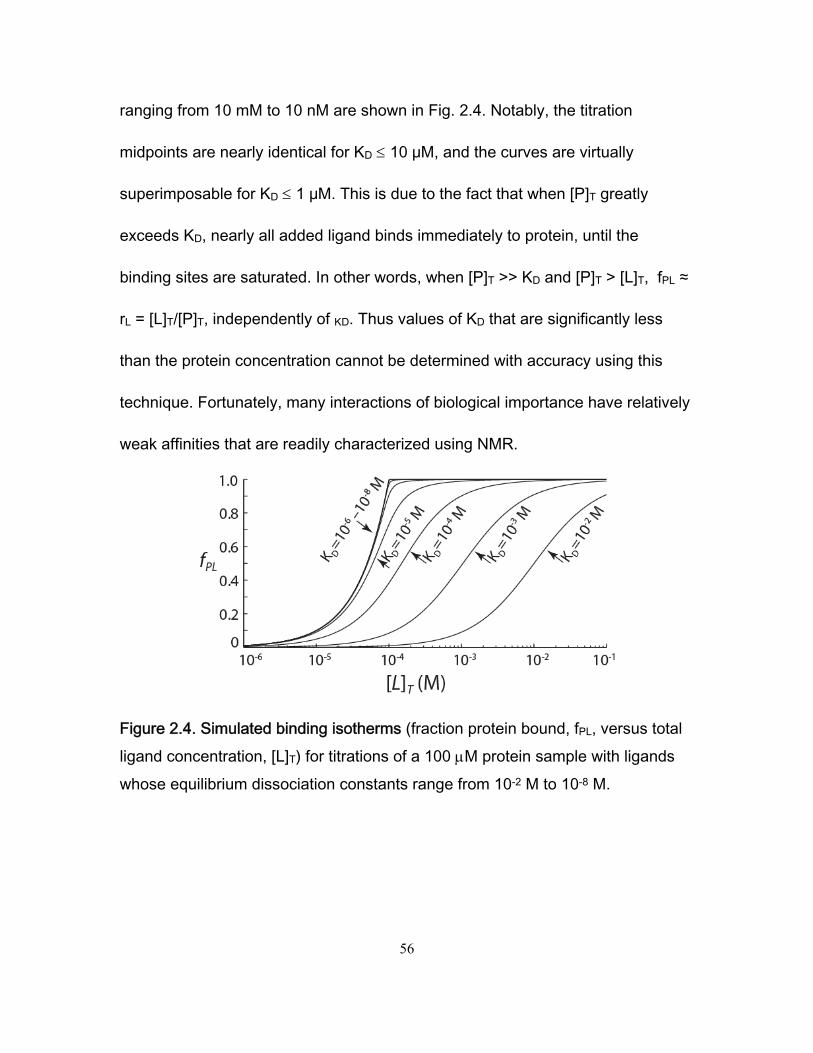
56
ranging from 10 mM to 10 nM are shown in Fig. 2.4. Notably, the titration
midpoints are nearly identical for KD 10 μM, and the curves are virtually
superimposable for KD 1 μM. This is due to the fact that when [P]T greatly
exceeds KD, nearly all added ligand binds immediately to protein, until the
binding sites are saturated. In other words, when [P]T >> KD and [P]T > [L]T, fPL ≈
rL = [L]T/[P]T, independently of KD. Thus values of KD that are significantly less
than the protein concentration cannot be determined with accuracy using this
technique. Fortunately, many interactions of biological importance have relatively
weak affinities that are readily characterized using NMR.
Figure 2.4. Simulated binding isotherms (fraction protein bound, fPL, versus total ligand concentration, [L]T) for titrations of a 100 M protein sample with ligands whose equilibrium dissociation constants range from 10-2 M to 10-8 M.
57
In the case of slow association/dissociation kinetics, NMR spectra obey the
expressions
0
,0
PL PL i PLT iL
VI L f
V V
0
,0
1P P i PLT iL
VI L f
V V
(2.7)
where IPL([L]T)i and IP([L]T)i are the peak intensities of residue i in the bound and
free forms for a given ligand concentration, [L]T, V0 is the initial sample volume,
VL is the volume of added ligand solution, λPL,i and λP,i are normalization
constants, and fPL is given by Equation 2.6. Peak intensities can be fitted
simultaneously (using Equation 2.7) to yield λPL,i and λP,i on a per-peak basis and
a single global value of KD. The term V0/(V0+VL) accounts for dilution of the
protein sample, with the assumption that peak intensity is directly proportional to
protein concentration.
In the case of fast association/dissociation kinetics, the displacement of peak i
from its initial location in the spectrum is given by the expression
,disp i PL iTL f , (2.8)
where fPL is again given by Equation 2.6, Δωi = ωPL,i – ωP,i, and ωPL,i, ωP,i are the
resonant frequencies of nucleus i in the bound and free states, respectively.
When 2D NMR datasets are employed, displacements in the two frequency
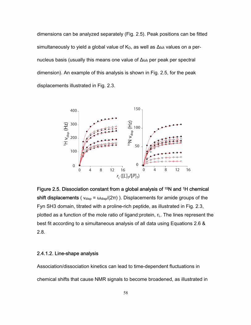
58
dimensions can be analyzed separately (Fig. 2.5). Peak positions can be fitted
simultaneously to yield a global value of KD, as well as Δωi values on a per-
nucleus basis (usually this means one value of Δωi per peak per spectral
dimension). An example of this analysis is shown in Fig. 2.5, for the peak
displacements illustrated in Fig. 2.3.
Figure 2.5. Dissociation constant from a global analysis of 15N and 1H chemical shift displacements ( νdisp = ωdisp/(2π) ). Displacements for amide groups of the Fyn SH3 domain, titrated with a proline-rich peptide, as illustrated in Fig. 2.3, plotted as a function of the mole ratio of ligand:protein, rL. The lines represent the best fit according to a simultaneous analysis of all data using Equations 2.6 & 2.8.
2.4.1.2. Line-shape analysis
Association/dissociation kinetics can lead to time-dependent fluctuations in
chemical shifts that cause NMR signals to become broadened, as illustrated in
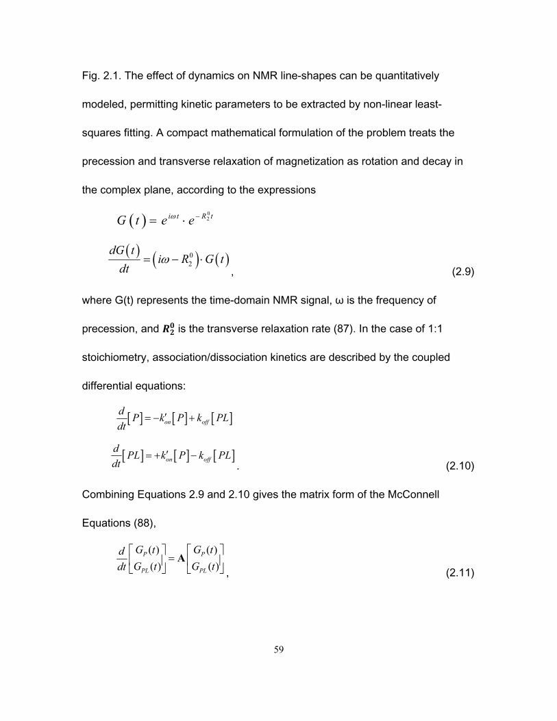
59
Fig. 2.1. The effect of dynamics on NMR line-shapes can be quantitatively
modeled, permitting kinetic parameters to be extracted by non-linear least-
squares fitting. A compact mathematical formulation of the problem treats the
precession and transverse relaxation of magnetization as rotation and decay in
the complex plane, according to the expressions
02R ti tG t e e
02
dG ti R G t
dt
, (2.9)
where G(t) represents the time-domain NMR signal, ω is the frequency of
precession, and is the transverse relaxation rate (87). In the case of 1:1
stoichiometry, association/dissociation kinetics are described by the coupled
differential equations:
on off
dP k P k PL
dt
on off
dPL k P k PL
dt
. (2.10)
Combining Equations 2.9 and 2.10 gives the matrix form of the McConnell
Equations (88),
( ) ( )
( ) ( )P P
PL PL
G t G tdG t G tdt
A
, (2.11)
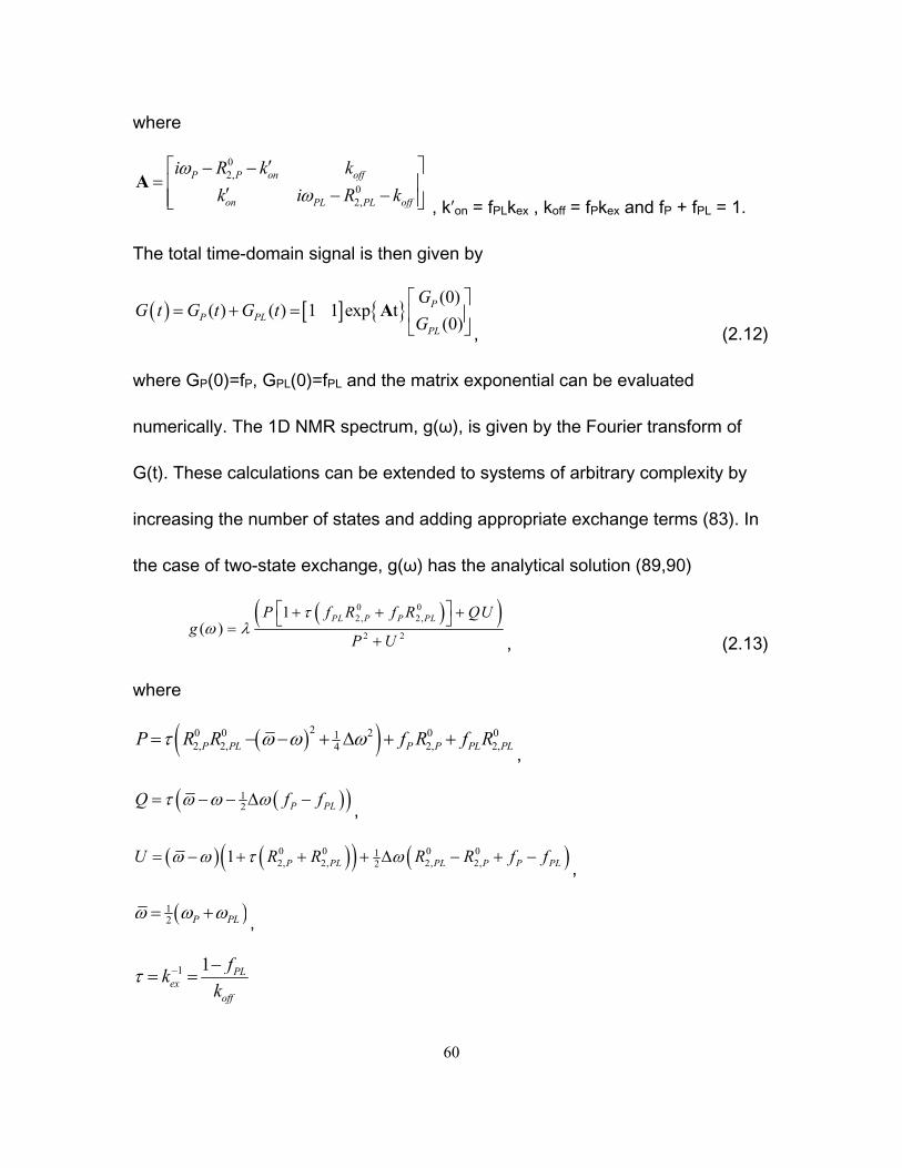
60
where
02,
02,
P P on off
on PL PL off
i R k k
k i R k
A
, kʹon = fPLkex , koff = fPkex and fP + fPL = 1.
The total time-domain signal is then given by
(0)
( ) ( ) 1 1 exp t(0)
PP PL
PL
GG t G t G t
G
A
, (2.12)
where GP(0)=fP, GPL(0)=fPL and the matrix exponential can be evaluated
numerically. The 1D NMR spectrum, g(ω), is given by the Fourier transform of
G(t). These calculations can be extended to systems of arbitrary complexity by
increasing the number of states and adding appropriate exchange terms (83). In
the case of two-state exchange, g(ω) has the analytical solution (89,90)
0 0
2, 2,
2 2
1( )
PL P P PLP f R f R QUg
P U
, (2.13)
where
20 0 2 0 012, 2, 2, 2,4P PL P P PL PLP R R f R f R
,
12 P PLQ f f ,
0 0 0 012, 2, 2, 2,21 P PL PL P P PLU R R R R f f
,
12 P PL ,
1 1 PLex
off
fk
k
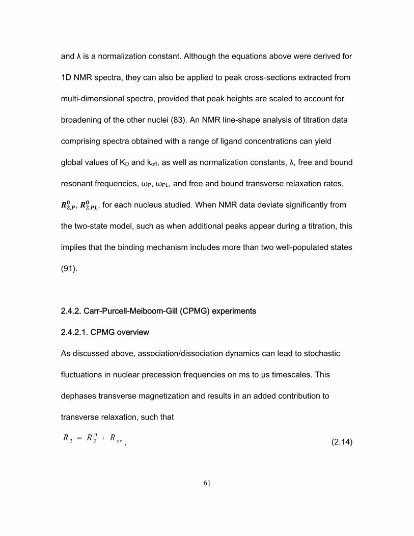
61
and λ is a normalization constant. Although the equations above were derived for
1D NMR spectra, they can also be applied to peak cross-sections extracted from
multi-dimensional spectra, provided that peak heights are scaled to account for
broadening of the other nuclei (83). An NMR line-shape analysis of titration data
comprising spectra obtained with a range of ligand concentrations can yield
global values of KD and koff, as well as normalization constants, λ, free and bound
resonant frequencies, ωP, ωPL, and free and bound transverse relaxation rates,
, , , , for each nucleus studied. When NMR data deviate significantly from
the two-state model, such as when additional peaks appear during a titration, this
implies that the binding mechanism includes more than two well-populated states
(91).
2.4.2. Carr-Purcell-Meiboom-Gill (CPMG) experiments
2.4.2.1. CPMG overview
As discussed above, association/dissociation dynamics can lead to stochastic
fluctuations in nuclear precession frequencies on ms to μs timescales. This
dephases transverse magnetization and results in an added contribution to
transverse relaxation, such that
02 2 e xR R R , (2.14)
62
where R2 is the observed transverse relaxation rate, Rex is the exchange
contribution, and is the relaxation rate in the absence of exchange. Line-
shape analyses fit R2, and thus Rex indirectly, since peak height is proportional to
1/R2 and the full width at half height is equal to R2/π. In contrast, Carr-Purcell-
Meiboom-Gill (CPMG) experiments can provide detailed dynamical exchange
information by studying Rex more directly (92,93). In the CPMG approach, R2 is
measured while Rex is suppressed with variable numbers of refocusing pulses
applied during a constant relaxation delay (Fig. 6a) (71). The dependence of R2,
and hence Rex, on the pulse repetition rate can be analyzed to extract the
populations, exchange rates and chemical shifts of interconverting states (94).
There are other advantages to the CPMG approach. Whereas, line-shape
analyses require a series of spectra be recorded as ligand is titrated into the
sample, CPMG experiments require only a single NMR sample. Furthermore,
CPMG experiments can yield detailed information on weakly-populated protein
states that are "invisible" in standard NMR correlation spectra (95).
The CPMG experiment is based on the Hahn spin-echo experiment, which
consists of two equal delays of length τ, during which magnetization precesses
(rotates) in the transverse plane, separated by a 180° refocusing pulse (τ-180-τ)
(96). A spin's precession is completely refocused during the spin echo, provided
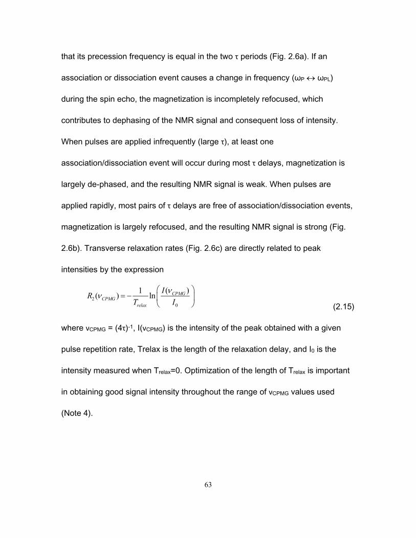
63
that its precession frequency is equal in the two τ periods (Fig. 2.6a). If an
association or dissociation event causes a change in frequency (ωP ωPL)
during the spin echo, the magnetization is incompletely refocused, which
contributes to dephasing of the NMR signal and consequent loss of intensity.
When pulses are applied infrequently (large τ), at least one
association/dissociation event will occur during most τ delays, magnetization is
largely de-phased, and the resulting NMR signal is weak. When pulses are
applied rapidly, most pairs of τ delays are free of association/dissociation events,
magnetization is largely refocused, and the resulting NMR signal is strong (Fig.
2.6b). Transverse relaxation rates (Fig. 2.6c) are directly related to peak
intensities by the expression
2
0
( )1( ) ln CPMG
CPMGrelax
IR
T I
(2.15)
where νCPMG = (4τ)-1, I(νCPMG) is the intensity of the peak obtained with a given
pulse repetition rate, Trelax is the length of the relaxation delay, and I0 is the
intensity measured when Trelax=0. Optimization of the length of Trelax is important
in obtaining good signal intensity throughout the range of νCPMG values used
(Note 4).
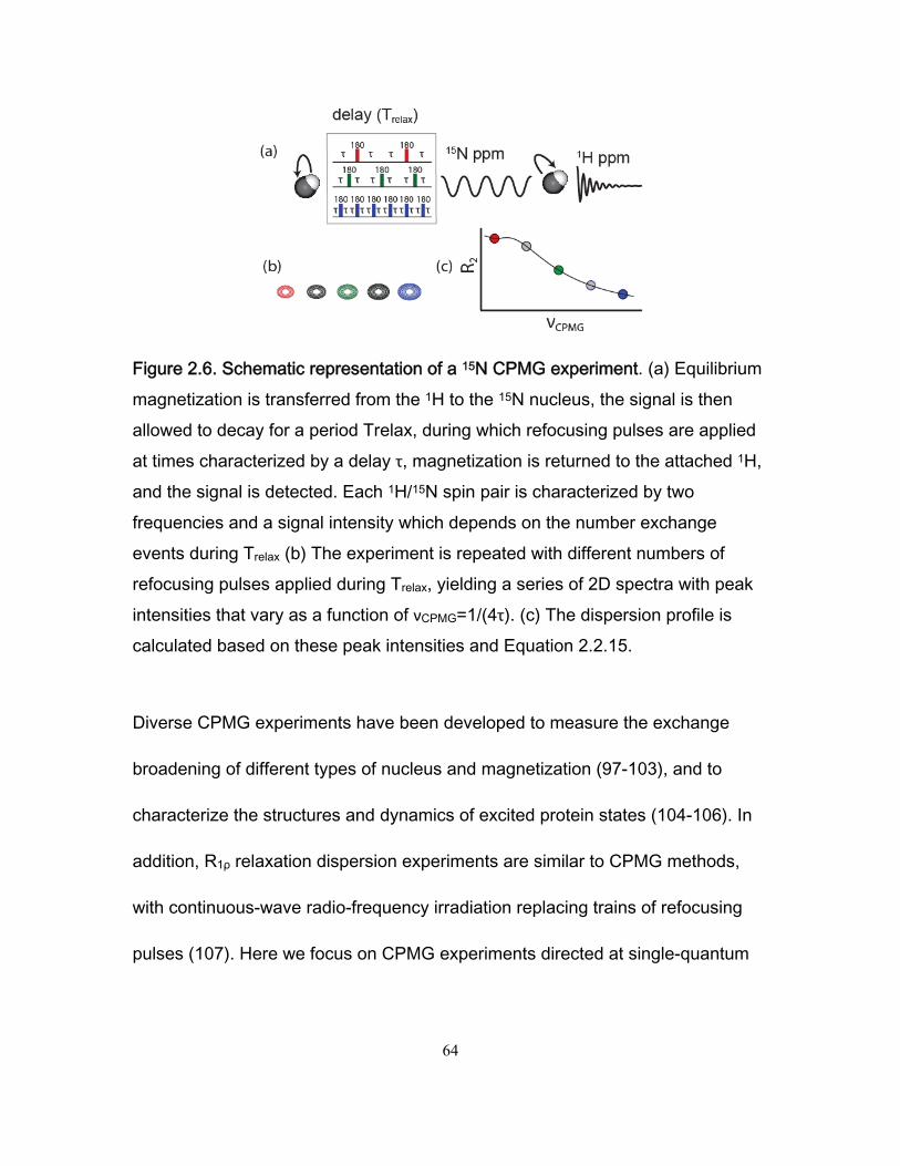
64
Figure 2.6. Schematic representation of a 15N CPMG experiment. (a) Equilibrium magnetization is transferred from the 1H to the 15N nucleus, the signal is then allowed to decay for a period Trelax, during which refocusing pulses are applied at times characterized by a delay τ, magnetization is returned to the attached 1H, and the signal is detected. Each 1H/15N spin pair is characterized by two frequencies and a signal intensity which depends on the number exchange events during Trelax (b) The experiment is repeated with different numbers of refocusing pulses applied during Trelax, yielding a series of 2D spectra with peak intensities that vary as a function of νCPMG=1/(4τ). (c) The dispersion profile is calculated based on these peak intensities and Equation 2.2.15.
Diverse CPMG experiments have been developed to measure the exchange
broadening of different types of nucleus and magnetization (97-103), and to
characterize the structures and dynamics of excited protein states (104-106). In
addition, R1ρ relaxation dispersion experiments are similar to CPMG methods,
with continuous-wave radio-frequency irradiation replacing trains of refocusing
pulses (107). Here we focus on CPMG experiments directed at single-quantum
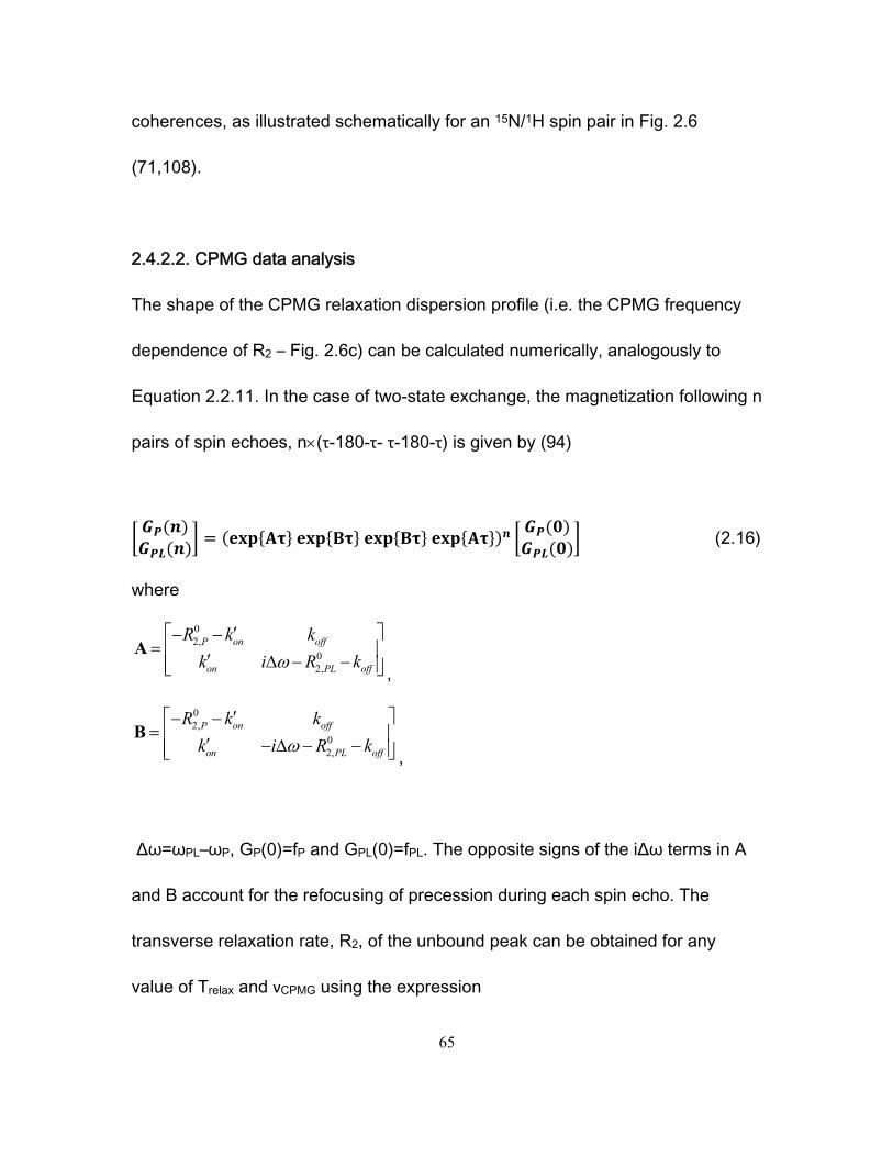
65
coherences, as illustrated schematically for an 15N/1H spin pair in Fig. 2.6
(71,108).
2.4.2.2. CPMG data analysis
The shape of the CPMG relaxation dispersion profile (i.e. the CPMG frequency
dependence of R2 – Fig. 2.6c) can be calculated numerically, analogously to
Equation 2.2.11. In the case of two-state exchange, the magnetization following n
pairs of spin echoes, n(τ-180-τ- τ-180-τ) is given by (94)
(2.16)
where
02,
02,
P on off
on PL off
R k k
k i R k
A
,
02,
02,
P on off
on PL off
R k k
k i R k
B
,
Δω=ωPL–ωP, GP(0)=fP and GPL(0)=fPL. The opposite signs of the iΔω terms in A
and B account for the refocusing of precession during each spin echo. The
transverse relaxation rate, R2, of the unbound peak can be obtained for any
value of Trelax and νCPMG using the expression
66
(2.17)
where τ = 1/ (4νCPMG) and n = νCPMG x Trelax.
If separate peaks are obtained for the free and bound forms (i.e. for systems in
the slow exchange regime), the R2 value for the bound peak can be obtained by
substituting GP with GPL in the expression above. It is assumed that , , in
the expressions above, since the intrinsic relaxation rates of the protein are
generally not dramatically affected by ligand binding, and it is not possible, in
general, to extract separate values for , and , from CPMG data (109)
(Note 5). This approach for calculating CPMG relaxation dispersion profiles can
be generalized to systems containing arbitrary numbers of states by extending
the matrices A and B of Equation 2.16 with additional chemical shift differences
(Δω) and relaxation rates (R2) along the diagonal together with exchange rate
constants in the appropriate elements (110).
In the case of two-state exchange, the transverse relaxation rate of the more
populated form (R2,A) is given by the analytical expression (111,112)
0 0 112, 2, 2,2 2 cosh cosh coshA CPMG A B ex CPMGR R R k D D
(2.18)
67
where
212 2 2
21D
,
2 22
4 CPMG
,
20 0 2 22, 2, 4A B B ex A ex A B exR R f k f k f f k ,
0 02, 2,2 A B B ex A exR R f k f k ,
, , 0.5,
, , 0.5PL
PL
P PL fA B
PL P f
.
This expression applies to the signal from the major form of the protein (i.e. to the
free state where ligand concentration is relatively low, and to the bound state
close to saturation). In the limit of fast exchange (kex >> Δω) this equation is well
approximated by the simpler expression (113)
0 0
2 2, 2,
41 tanh
4ex CPMG ex
CPMG P P PL PLex ex CPMG
kR f R f R
k k
, (2.19)
where Φex = fPfPLΔω2.
A typical CPMG experiment consists of series of roughly ten to twenty 2D
correlation spectra obtained with a range of νCPMG values and yielding R2 values
for each amide, calculated using Equation 2.2.15. For systems in intermediate
68
timescale exchange, the analysis proceeds with non-linear least-squares fitting of
R2 values using Equation 2.2.18, while for systems in fast exchange Equation
2.2.19 is employed. The exchange regime can be determined from an inspection
of line-shapes throughout the titration, as discussed in Section 2.1. Series of
experiments should be performed at a minimum of two different static magnetic
field strengths under otherwise identical conditions (114) (Note 3). Additional
information useful in selecting the appropriate equation for analyses is provided
by the dependence of exchange broadening at different static field strengths as
expressed by the parameter α (115)
0
ln
lnexd R
d B
, (2.20)
where B0 is the NMR spectrometer field strength and Rex is the exchange
contribution to transverse relaxation. Rex may be estimated as the difference
between the experimental R2 values obtained with maximal and minimal νCPMG
(i.e. the reduction in R2 with increasing frequency). In the intermediate exchange
regime, α ≈ 1, and Rex scales roughly linearly with field strength. In the fast
exchange regime, α ≈ 2, and Rex scales as the square of the field strength. Note
that different peaks may be in different exchange regimes depending on their
values of Δω, such that data for peaks with smaller Δω values may obey the fast-
69
exchange Equation 2.2.19, while peaks with larger Δω values may require the
intermediate exchange Equation 2.2.18.
Fits of multiple-field data from one residue using Equation 2.2.18 yield the
parameters kex, fPL, and Δω2, and an value for each spectrometer field
strength (again assuming that , , )(Fig. 2.7a). The dissociation
rate constant is then given by koff = (1-fPL)kex and the second-order association
rate constant is calculated as kon=KD/koff. Fits with the fast-exchange Equation
2.2.19 yield the parameters kex, Φex, and values of (Fig. 2.7b). Note that in the
fast exchange regime, fPL and Δω2 cannot be determined separately, as both are
subsumed into Φex. In this case, the value of fPL can be determined from
observed peak displacements relative to the maximum peak displacements
(ligand-free versus ligand-saturated spectra) according to Equation 2.8, or from
an analysis of dependence of Φex on Δω2 (Note 7). More accurate results can be
obtained by fitting dispersion profiles for all residues simultaneously, with values
of kex and fPL optimized globally and values of Δω2 and extracted on a per-
residue basis (116). If exchange for all residues is in the fast regime, then only
kex is determined globally, while Φex and are obtained on a per-residue basis.
The extracted values of Δω2 or Φex can be used to validate the use of the two-
state exchange model (Note 7).
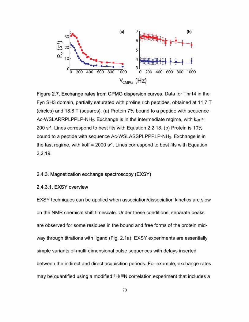
70
Figure 2.7. Exchange rates from CPMG dispersion curves. Data for Thr14 in the Fyn SH3 domain, partially saturated with proline rich peptides, obtained at 11.7 T (circles) and 18.8 T (squares). (a) Protein 7% bound to a peptide with sequence Ac-WSLARRPLPPLP-NH2. Exchange is in the intermediate regime, with koff ≈ 200 s-1. Lines correspond to best fits with Equation 2.2.18. (b) Protein is 10% bound to a peptide with sequence Ac-WSLASSPLPPPLP-NH2. Exchange is in the fast regime, with koff ≈ 2000 s-1. Lines correspond to best fits with Equation 2.2.19.
2.4.3. Magnetization exchange spectroscopy (EXSY)
2.4.3.1. EXSY overview
EXSY techniques can be applied when association/dissociation kinetics are slow
on the NMR chemical shift timescale. Under these conditions, separate peaks
are observed for some residues in the bound and free forms of the protein mid-
way through titrations with ligand (Fig. 2.1a). EXSY experiments are essentially
simple variants of multi-dimensional pulse sequences with delays inserted
between the indirect and direct acquisition periods. For example, exchange rates
may be quantified using a modified 1H/15N correlation experiment that includes a
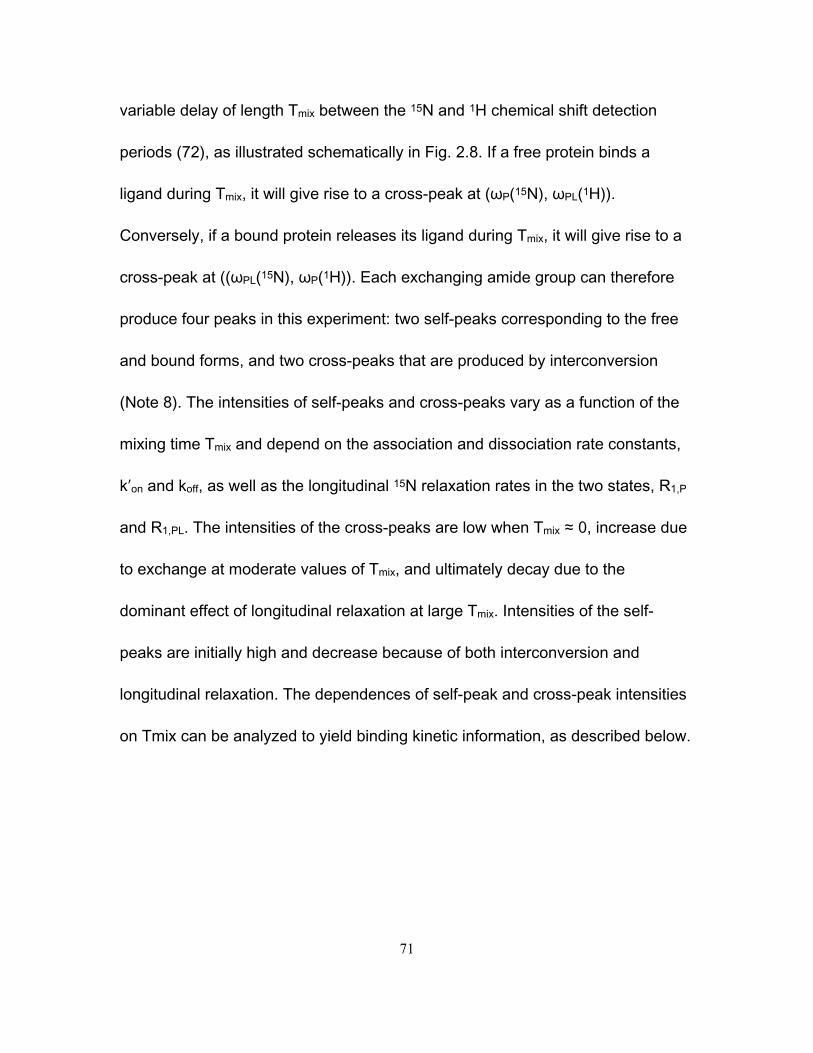
71
variable delay of length Tmix between the 15N and 1H chemical shift detection
periods (72), as illustrated schematically in Fig. 2.8. If a free protein binds a
ligand during Tmix, it will give rise to a cross-peak at (ωP(15N), ωPL(1H)).
Conversely, if a bound protein releases its ligand during Tmix, it will give rise to a
cross-peak at ((ωPL(15N), ωP(1H)). Each exchanging amide group can therefore
produce four peaks in this experiment: two self-peaks corresponding to the free
and bound forms, and two cross-peaks that are produced by interconversion
(Note 8). The intensities of self-peaks and cross-peaks vary as a function of the
mixing time Tmix and depend on the association and dissociation rate constants,
kʹon and koff, as well as the longitudinal 15N relaxation rates in the two states, R1,P
and R1,PL. The intensities of the cross-peaks are low when Tmix ≈ 0, increase due
to exchange at moderate values of Tmix, and ultimately decay due to the
dominant effect of longitudinal relaxation at large Tmix. Intensities of the self-
peaks are initially high and decrease because of both interconversion and
longitudinal relaxation. The dependences of self-peak and cross-peak intensities
on Tmix can be analyzed to yield binding kinetic information, as described below.
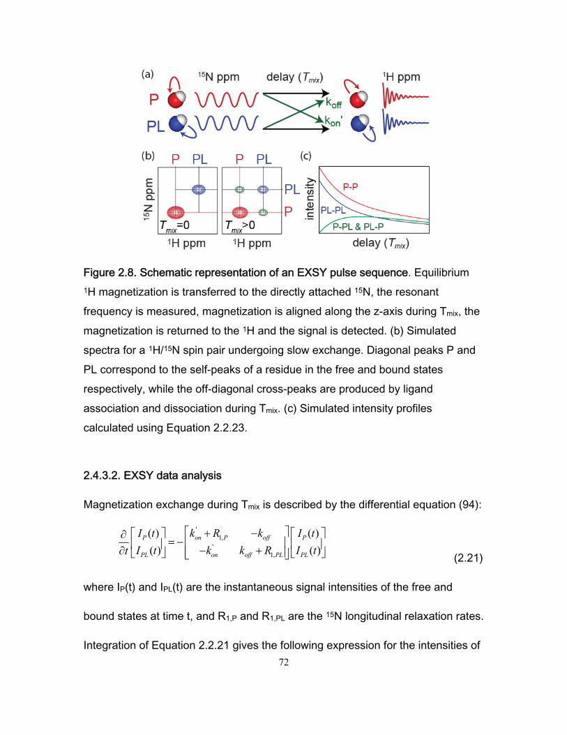
72
Figure 2.8. Schematic representation of an EXSY pulse sequence. Equilibrium 1H magnetization is transferred to the directly attached 15N, the resonant frequency is measured, magnetization is aligned along the z-axis during Tmix, the magnetization is returned to the 1H and the signal is detected. (b) Simulated spectra for a 1H/15N spin pair undergoing slow exchange. Diagonal peaks P and PL correspond to the self-peaks of a residue in the free and bound states respectively, while the off-diagonal cross-peaks are produced by ligand association and dissociation during Tmix. (c) Simulated intensity profiles calculated using Equation 2.2.23.
2.4.3.2. EXSY data analysis
Magnetization exchange during Tmix is described by the differential equation (94):
'1,
'1,
( ) ( )
( ) ( )P on P off P
PL on off PL PL
I t k R k I t
I t k k R I tt
(2.21)
where IP(t) and IPL(t) are the instantaneous signal intensities of the free and
bound states at time t, and R1,P and R1,PL are the 15N longitudinal relaxation rates.
Integration of Equation 2.2.21 gives the following expression for the intensities of
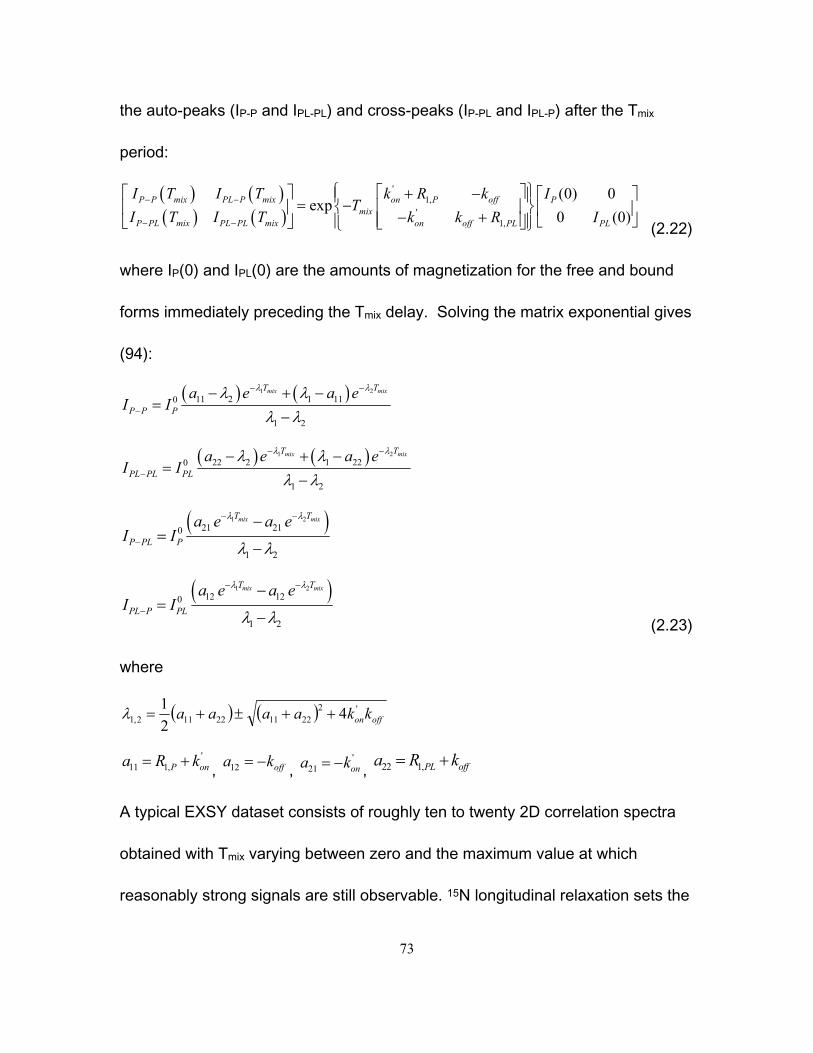
73
the auto-peaks (IP-P and IPL-PL) and cross-peaks (IP-PL and IPL-P) after the Tmix
period:
'1,
'1,
(0) 0exp
0 (0)P P mix PL P mix on P off P
mixP PL mix PL PL mix on off PL PL
I T I T k R k IT
I T I T k k R I
(2.22)
where IP(0) and IPL(0) are the amounts of magnetization for the free and bound
forms immediately preceding the Tmix delay. Solving the matrix exponential gives
(94):
1 211 2 1 110
1 2
mix mixT T
P P P
a e a eI I
1 222 2 1 220
1 2
mix mixT T
PL PL PL
a e a eI I
1 221 210
1 2
mix mixT T
P PL P
a e a eI I
1 212 120
1 2
mix mixT T
PL P PL
a e a eI I
(2.23)
where
offonkkaaaa '2221122112,1 4
2
1
'
11 1,P ona R k , offka 12 , '
21 ona k , 22 1,PL offa R k
A typical EXSY dataset consists of roughly ten to twenty 2D correlation spectra
obtained with Tmix varying between zero and the maximum value at which
reasonably strong signals are still observable. 15N longitudinal relaxation sets the
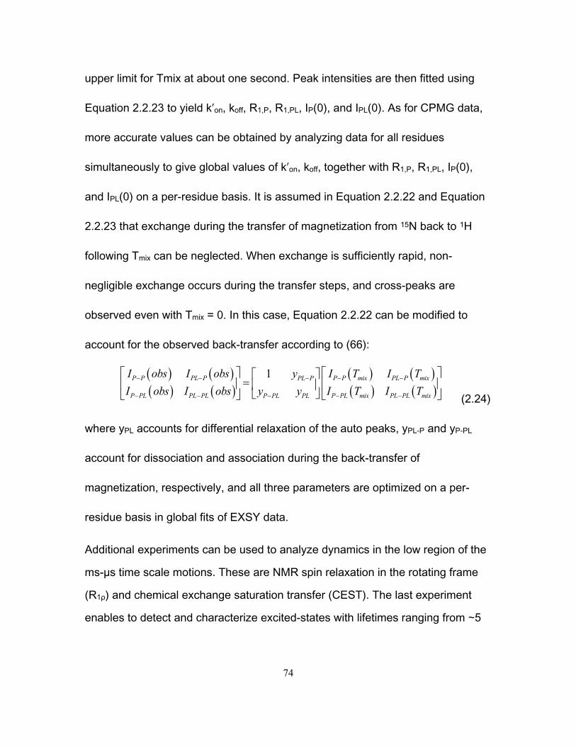
74
upper limit for Tmix at about one second. Peak intensities are then fitted using
Equation 2.2.23 to yield kʹon, koff, R1,P, R1,PL, IP(0), and IPL(0). As for CPMG data,
more accurate values can be obtained by analyzing data for all residues
simultaneously to give global values of kʹon, koff, together with R1,P, R1,PL, IP(0),
and IPL(0) on a per-residue basis. It is assumed in Equation 2.2.22 and Equation
2.2.23 that exchange during the transfer of magnetization from 15N back to 1H
following Tmix can be neglected. When exchange is sufficiently rapid, non-
negligible exchange occurs during the transfer steps, and cross-peaks are
observed even with Tmix = 0. In this case, Equation 2.2.22 can be modified to
account for the observed back-transfer according to (66):
1P P PL P P P mix PL P mixPL P
P PL PL PL P PL mix PL PL mixP PL PL
I obs I obs I T I Ty
I obs I obs I T I Ty y
(2.24)
where yPL accounts for differential relaxation of the auto peaks, yPL-P and yP-PL
account for dissociation and association during the back-transfer of
magnetization, respectively, and all three parameters are optimized on a per-
residue basis in global fits of EXSY data.
Additional experiments can be used to analyze dynamics in the low region of the
ms-µs time scale motions. These are NMR spin relaxation in the rotating frame
(R1ρ) and chemical exchange saturation transfer (CEST). The last experiment
enables to detect and characterize excited-states with lifetimes ranging from ∼5
75
to 50 ms. However, these experiments are out of the scope of the present
document.
2.5. Notes
2.5.1. NMR Titrations
1. An important consideration when performing NMR titration experiments is the
selection of ligand concentrations. If an approximate affinity constant is already
known, the appropriate ligand concentrations can be chosen using Equation 2.6
so as to adequately define the saturated baseline and the curvature of the
binding isotherm. The situation is more complicated if no prior information on the
affinity is available. This is particularly true in the case of fast exchange, since
peak displacements can only be quantitatively related to fPL once the saturated
baseline is obtained, i.e. once the titration is complete. In this case, it is advisable
to collect several (5) spectra over ligand:protein ratios (rL) from 0 to about 1.5. If
the interaction is of high affinity ([P]T > KD) saturation will be reached over this
interval. If peak displacements vary linearly with [L]T past the stoichiometric
equivalence point (rL=1), then KD > [P]T and larger increments of [L]T can be used
for additional titration points.
2. When performing titrations it is critical that the ligand and protein solutions are
mixed thoroughly and that sample loss during the mixing procedure is minimized.
76
We recommend withdrawing the sample from the NMR tube completely, using a
Hamilton syringe or an NMR long-tip pipette, and transferring it to small (≈1.5
mL) sample tube. Ligand can then be added using a standard pipettor, the
sample can be thoroughly mixed, spun down, and returned to the NMR tube
using the syringe. It is preferable to use the same NMR tube, sample tube, and
syringe for every titration step (without rinsing) in order to minimize loss of the
sample.
2.5.2. CPMG experiments
3. Temperature control is a major concern in studies of relaxation, particularly
when performing CPMG studies as data from more than one spectrometer are
analyzed assuming that protein dynamics (and hence temperatures) are identical
in all instruments. Calibration curves can be constructed for each NMR probe
using perdeutarated methanol to measure the true sample temperature (117). In
this case, T(K) = -16.7467 (Δδ)2 - 52.5130 Δδ + 419.1381, (Δδ = δOH – δCHD2)
(118), where δ is expressed in ppm. Alternatively, a non-magnetic digital
thermometer may be inserted directly into the NMR probe. Another issue is
heating caused by RF pulses, particularly when proton decoupling is applied
during the relaxation delay (108). This effect can be assayed by measuring the
water resonance frequency (unlocked) before and after several minutes of
77
irradiation with the pulse sequence, as the water resonance shifts by
approximately -.01 ppm K-1 (119). The temperature setting of the spectrometer
can then be adjusted by a compensatory amount (usually by about 0.1 to 0.2 °C)
4. A critical parameter when performing CPMG relaxation dispersion experiments
is the length of the constant relaxation delay, Trelax. Longer values of Trelax allow
more time for exchange broadening to occur, whereas shorter values lead to less
signal loss overall and more intense peaks. Therefore a compromise must be
reached between maximizing the sensitivity to Rex and optimizing signal strength.
We find that a good balance is achieved when the spectrum obtained with the
maximum νCPMG is about half as intense as that obtained with Trelax=0. This
corresponds to an optimal value of Trelax ≈ ln{2}/ (e.g., 40 ms for = 17 s-1).
One caveat to this rule is that Trelax periods longer than 40ms are generally not
used, in order to limit amplifier loads, even when values are small.
5. Alternatively, R2 values can be measured separately for the ligand-free and
ligand-saturated forms of the protein and then held fixed in analyses of CPMG
data.
78
6. Some NMR cold-probes exhibit RF pulse-dependent artifacts, such that the
sensitivity decreases (and apparent R2 increases) with increasing νCPMG. In the
case of Varian cold probes, it has been found that this can be suppressed by
applying CW irradiation to 15N nuclei prior to each transient for a variable time
period, TCW, given by
relax
CPMG
iCPMGCPMGiCW TT
max
max
)(
)()()(
where (νCPMG)max is the largest value of νCPMG employed in a dispersion series,
typically 1000 Hz (66). A compensation power level 8 dB below that of the CPMG
pulse train typically provides excellent artifact suppression at all fields and
temperatures.
7. In the case of two-state exchange, Δω2 values obtained from titration
experiments (i.e. squared maximum peak displacements) should equal Δω2
parameters extracted from CPMG data using Equation 2.2.18, and should
correlate linearly Φex values obtained using Equation 2.2.19 (66). If Φex values for
all residues are plotted as function of titration-derived Δω2 values, the slope is
equal to fPfPL = (1-fPL)fPL. If these correlations are not observed experimentally, it
may be taken as evidence for the existence of additional millisecond-timescale
exchange phenomena, i.e. dynamics involving more than two states. In this case,
79
multi-state binding parameters can be extracted by simultaneously fitting CPMG
data obtained with different levels of ligand saturation (59).
2.5.3. EXSY experiments
8. EXSY experiments provide a convenient means for transferring spectral
assignments from the free to the bound protein NMR spectrum, for systems that
are in slow exchange. When association/dissociation kinetics are rapid,
transferring assignments is a trivial process, since each peak gradually moves
from the ligand-free frequencies to the ligand-saturated frequencies over the
course of the titration. In contrast, for a slowly-exchanging system, it can be
challenging to associate each gradually appearing peak with its corresponding
disappearing peak in the titration data. The locations of exchange cross-peaks in
EXSY spectra for a partially-saturated protein sample, thus, identify pairs of self
peaks that are produced by the same amide group in the free and bound states
(3).
80
3. Electrostatic interactions in the binding pathway of a transient protein complex
studied by NMR and isothermal titration calorimetry
I have coauthored this article with:
Anthony Mittermaier
This article was published in:
Meneses, E., and Mittermaier, A. Electrostatic interactions in the binding pathway of a transient protein complex studied by NMR and isothermal titration calorimetry. J. Biol. Chem. 2014 289: 27911-27923. First Published on August 13, 2014.
81
Keywords: Protein dynamics; Src Homology 3 (SH3) domain; Nuclear Magnetic Resonance (NMR); Isothermal Titration Calorimetry (ITC); Carr–Purcell–Meiboom–Gill (CPMG) relaxation dispersion
Background: Electrostatic interactions are known accelerate binding in protein complexes with long lifetimes (min-hr). Results: NMR and calorimetry were used to characterize binding kinetics in short-lived (≈ms) protein-peptide complexes. Conclusion: Electrostatic enhancement is much less and basal (electrostatic-free) association rates are greater than previously observed. Significance: Electrostatics may play different roles in short-lived and long-lived protein complexes. 3.1. Abstract
Much of our knowledge of protein binding pathways is derived from extremely
stable complexes that interact very tightly, with lifetimes of hours to days. Much
less is known about weaker interactions and transient complexes, since these
are challenging to characterize experimentally. Nevertheless, these types of
interactions are ubiquitous in living systems. The combination of NMR relaxation
dispersion CPMG experiments and isothermal titration calorimetry allows the
quantification of rapid binding kinetics for complexes with sub-millisecond
lifetimes that are difficult to study using conventional techniques. We have used
this approach to investigate the binding pathway of the Src Homology 3 (SH3)
82
domain from the Fyn tyrosine kinase, which forms complexes with peptide
targets whose lifetimes are on the order of about a millisecond. Long-range
electrostatic interactions have been shown to play a critical role in the binding
pathways of tightly-binding complexes. The role of electrostatics in the binding
pathways of transient complexes is less well understood. Similarly to previously-
studied tight complexes, we find that SH3 domain association rates are
enhanced by long-range electrostatics, while short-range interactions are formed
late in the docking process. However, the extent of electrostatic association rate
enhancement is several orders of magnitudes less, while the electrostatic-free
basal association rate is significantly greater. Thus the SH3 domain is far less
reliant on electrostatic enhancement to achieve rapid association kinetics than
are previously studied systems. This suggests there may be overall differences in
the role played by electrostatics in the binding pathways of extremely stable
versus transient complexes.
3.2. Introduction
Many biological processes rely on the rapid formation of protein-ligand
complexes (120-124). Consequently there has been great interest in elucidating
the mechanisms through which binding partners are able to efficiently recognize
each other in solution and adopt the correct conformations, relative positions and
83
orientations to form native stereo-specific complexes. This has been addressed
theoretically (16,125), by computer simulation (126,127), and experimentally
(120,124,128,129). The association process is typically broken down into at least
two steps. In the first step, the binding partners encounter each other through a
random collision. For the small fraction of collisions in which the binding surfaces
are correctly aligned (as few as 1 in 105), the molecules proceed to the second
step and dock to form the native stereo-specific complex (20). If the docking step
occurs much more rapidly than the timescale of productive intermolecular
collisions, the reaction is said to be “diffusion-controlled” and the association rate
is viscosity-dependent (16). When binding is diffusion-controlled, the protein and
ligand pass through a free energy maximum en route to the bound state in which
translational-rotational entropy is reduced with little compensation from favorable
interactions (20,130). The ensemble of conformations at this free energy
maximum has been referred to as an "encounter complex" (16), "transient
complex" (131), or "transition state" (132). We shall use the term “transition
state” throughout. For these systems, binding is essentially two-state, such that
significant populations are observed only for the free and/or bound states, and a
negligible fraction of molecules populate the high-energy transition state at any
one time. Note that the two-state diffusion-controlled binding mechanism is
compatible with conformational changes occurring after the transition state,
84
provided that they proceed sufficiently rapidly (133). Additionally, transient
conformational reorganization can occur prior to the intermolecular collision,
leading to a “gated” diffusion-controlled binding mechanism (134). In either case,
the structure of the transition state is key to understanding the binding pathway,
as it represents a kinetic bottleneck. Interactions that stabilize the transition state
accelerate molecular association rates (16,131,132).
A variety of interactions have been proposed to contribute to the stability of
transition states, including non-specific hydrogen bonding, van der Waals
interactions, non-polar desolvation (desolvation of non-polar residues), long-
range electrostatic interactions, (16,135-137) or subsets of native bound-like
interactions (138). The role of electrostatics in binding pathways has been
particularly well studied. For a number of systems including barnase/barstar
(124), E9/Im9 (128), IL4/IL4BP (129), and Fas/AchE (120), it has been found that
electrostatic stabilization of weakly-specific transition states can accelerate
association by up to 4 or more orders of magnitude, compared to the basal rate
(132). A combination of experimental and computational studies has led to a
picture of the transition state in which the binding partners remain solvent
separated and interact almost exclusively by long-range electrostatics (132,139).
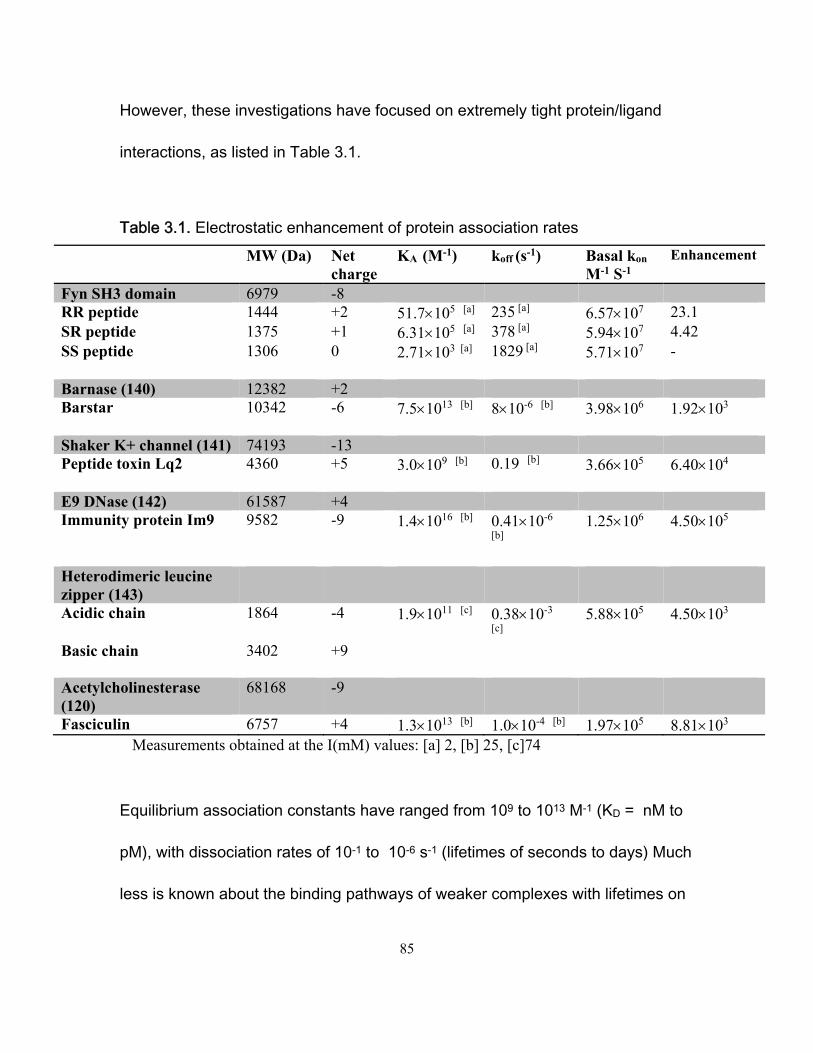
85
However, these investigations have focused on extremely tight protein/ligand
interactions, as listed in Table 3.1.
Table 3.1. Electrostatic enhancement of protein association rates MW (Da) Net
charge KA (M-1) koff (s-1) Basal kon
M-1 S-1 Enhancement
Fyn SH3 domain 6979 -8 RR peptide 1444 +2 51.7105 [a] 235 [a] 6.57107 23.1 SR peptide 1375 +1 6.31105 [a] 378 [a] 5.94107 4.42 SS peptide 1306 0 2.71103 [a] 1829 [a] 5.71107 - Barnase (140) 12382 +2 Barstar 10342 -6 7.51013 [b] 810-6 [b] 3.98106 1.92103 Shaker K+ channel (141) 74193 -13 Peptide toxin Lq2 4360 +5 3.0109 [b] 0.19 [b] 3.66105 6.40104 E9 DNase (142) 61587 +4 Immunity protein Im9 9582 -9 1.41016 [b] 0.4110-6
[b] 1.25106 4.50105
Heterodimeric leucine zipper (143)
Acidic chain 1864 -4 1.91011 [c] 0.3810-3
[c] 5.88105 4.50103
Basic chain 3402 +9 Acetylcholinesterase (120)
68168 -9
Fasciculin 6757 +4 1.31013 [b] 1.010-4 [b] 1.97105 8.81103 Measurements obtained at the I(mM) values: [a] 2, [b] 25, [c]74
Equilibrium association constants have ranged from 109 to 1013 M-1 (KD = nM to
pM), with dissociation rates of 10-1 to 10-6 s-1 (lifetimes of seconds to days) Much
less is known about the binding pathways of weaker complexes with lifetimes on
86
the order of milliseconds. These types of short-lived protein interactions are
abundant in nature, raising the important question: to what extent do long-lived
and short-lived complexes follow similar binding pathways? In what follows, we
will use “long-lived” to refer to complexes that bind with <nM KD and have
lifetimes on the order of minutes or longer. We will use “short-lived” to refer to
complexes with ≥M KD and lifetimes on the order of milliseconds. Several
studies of short-lived complexes have derived structural models of transient
complexes that precede formation of the fully-bound state (59,144,145). However
these investigations did not extract kinetic parameters nor identify the
interactions governing association rates, which is key to understanding binding
pathways.
The binding kinetics of short-lived complexes are challenging to measure
experimentally. In typical stop-flow binding measurements, the protein and ligand
are rapidly mixed and the extent of the reaction is monitored as a function of time
using techniques including spectroscopic absorbance (138), fluorescence
(128,140,146), enzymatic activity (120,147,148) and surface plasmon resonance
(149,150). These techniques are limited by the requirement that the lifetimes of
the free and bound states must be several-fold longer than the time required to
completely mix the protein and ligand solutions, otherwise the reaction proceeds
nearly to completion before the start of the measurement period.
87
The combination of Nuclear Magnetic Resonance (NMR) spectroscopy and
Isothermal Titration Calorimetry (151) can characterize binding kinetics that are
too rapid for standard stop-flow techniques, on the order of 104 s-1 (152). In this
approach, a sub-stoichiometric amount of ligand is added to a protein sample
whose signals are monitored by NMR spectroscopy. The resulting dynamical
exchange between the free and bound states modulates the chemical shifts of
nuclei in the protein on the ms to s timescale, leading to signal broadening. The
broadening is quantified by NMR relaxation dispersion experiments (153-155)
which yield the dissociation rate constant, koff. The equilibrium association
constant of the interaction, KA, is determined by ITC or NMR titration
experiments. The second-order association rate constant is then given by
on A offk K k . These two parameters report on the binding pathway as KA is
related to the free energy difference between the free and bound states while kon
is related to the free energy difference between the free state and the transition
state.
SH3 domains are typical of weakly-binding proteins that form short-lived
complexes. These ~60 amino acid modules are found in the context of larger
multi-domain proteins and mediate protein/protein interactions in signal
transduction pathways (156,157). The type I ligand recognized by many SH3
domains comprises a short peptide sequence: +xPxP where P is proline, is
88
a hydrophobic amino acid, x is any amino acid, and + is a positively-charged
residue, typically arginine or lysine (157). The positions in the motif are
numbered -3 to 3 such that the conserved + occupies site –3. Dissociation
constants for SH3 domains are usually on the order of M and the lifetimes of
their complexes are on the order of ms (152,158). We previously used NMR and
ITC to study the binding kinetics of the SH3 domain from the Fyn tyrosine kinase.
We showed that this protein binds a type I target peptide in a two-state manner
with ms-timescale kinetics and a temperature dependence of kon that is
consistent with diffusion-limited association (152). In the current study, we have
focused on how positively charged residues within the SH3 binding motif and
negatively-charged residues in the binding site on the SH3 domain interact to
influence association kinetics. Three different dodecapeptides were employed:
one with a typical type I consensus motif with the conserved R–3 preceded by S–4
(SR, net charge +1), a second containing R–4R–3 (RR, net charge +2), and a third
containing S–4S–3 (SS, net charge 0). We analyzed the contributions of the
conserved R-3 and “extra” R-4 residues to the stabilities of the fully-bound and
transition states by comparing the binding affinities and association rates of the
RR, SR, and SS peptides. Data were extrapolated to both zero ionic strength,
where long-range electrostatic interactions are maximal, and to infinite ionic
strength, where long-range electrostatics are fully attenuated. We find that the
89
conserved R-3 and the “extra” R-4 residues stabilize both the encounter and fully-
bound complexes via similar long-range electrostatic interactions, which implies
that the Fyn SH3 domain and peptide are fairly close in the transition state.
Notably, R-3 additionally stabilizes the bound state via short-range interactions
that are not screened by adding salt. Likely candidates include a network of salt-
bridges and hydrogen bonds previously observed for this residue in the bound
complex by NMR (159) and X-ray crystallography (PDB 4EIK). These short range
interactions involving R-3 are not present in the transition state and are only made
after the molecules have crossed the free energy barrier, near the end of the
binding pathway. Thus the SH3/peptide transition state is fairly compact and
stabilized primarily by long-range electrostatic interactions, as seen for other
protein/ligand systems (124,131,132,139). However, there are surprising
differences between the system studied here and the high-affinity long-lived
complexes investigated previously. We find that the electrostatic-free basal
association rate for this system is significantly greater while the electrostatic
association rate enhancement is several orders of magnitude less. This result
suggests that short-lived complexes may rely less on electrostatic enhancement
to achieve rapid binding than do high affinity long-lived complexes.
90
3.3. Materials and methods
Protein and peptide preparation - Wild-type chicken Fyn SH3 domain (residues
81 to 148) was expressed and purified as described previously (160). RR (Ac-
WSLAR–4R–3P–2L–1P0P1L2P3-NH2), SR (Ac-WSLAS–4R–3P–2L–1P0P1L2P3-NH2))
and SS (Ac-WSLAS–4S–3P–2L–1P0P1L2P3-NH2) peptides were purchased from the
Sheldon Biotechnology Centre (McGill, Montreal), and purified to homogeneity by
reverse-phase HPLC. Protein and peptide samples were dialyzed against 5 mM
MES pH 6.0 at the desired NaCl concentration. For ionic strength calculations, it
was assumed that the buffer contributed 2.57 mM charged ions. Most
experiments were performed at 40°C. This temperature was chosen to optimize
the NMR CPMG relaxation dispersion profiles obtained with the RR and SR
peptides, and lies within the physiological temperature range of 40-42 °C (161).
3.3.1. ITC
Titrations were performed at 40ºC using a VP-ITC instrument (MicroCal LLC,
Northampton, MA). Measurements were taken in triplicate for each NaCl
concentration and consisted of 56 injections of 5 μL. RR peptide data were
collected at 0.00, 0.01 0.03, 0.05, 0.10, 0.20, 0.30, 0.40, 0.50, 1.00, 1.50, and
2.00 M NaCl. For the SR and the SS peptide measurements were taken at 0.00,
0.03, 0.20 and 0.30 M NaCl.Titrations were repeated for the SS peptide at 20 °C.
91
Data were fitted using the one-set-of-independent-sites model in the Origin
Software package (OriginLab, Northampton, MA) and in-house MATLAB scripts
(MATLAB R2013a, The MathWorks, Natick, MA).
3.3.2. NMR
1H-15N HSQC titration spectra, referenced to an internal DSS standard (162),
were collected at 40 °C and 800 MHz for samples containing approximately 0.3
mM protein and 16 different peptide concentrations. In the case of the SS peptide
titration, chemical shift peak trajectories were fit globally according to (10):
212 4free bound free b b R
(3.1)
where free,bound are the chemical shifts of the free and bound protein,
R=[peptide]total/[protein]total, and b=1+R+(KA[protein]total)–1.
1H-decoupled 15N CPMG experiments (155) with power compensation schemes
(152) were performed at 40°C and 500 and 800 MHz on 1 mM samples of the
Fyn SH3 domain, free in solution (0M NaCl), in the presence of 0.1 mM SS, SR,
and RR peptides (0, 0.2, 0.3 M NaCl) and with saturating amounts of the RR
peptide (0 M NaCl). Measurements were repeated at 20 °C for the SH3 domain
alone (0 M NaCl) and in the presence of 0.1 mM SS peptide (0, 0.2, 0.3 M NaCl).
Experiments employed a constant relaxation delay, Trelax, of 40 ms and twenty-
92
three values of νCPMG = 1/(2τCP) ranging from 25 to 1000 Hz, where τCP is the
delay between consecutive pulses. Transverse relaxation rates, R2, were
calculated for each cross-peak signal at each νCPMG value according to:
0
exp2 ln
1
I
I
TR CPMG
relaxCPMG
(3.2)
where I(CPMG) is the peak intensity at a given value of νCPMG and I0 is the signal
intensity with Trelax=0. The experimental uncertainties in peak intensities (I) were
considered to be the same for all values of CPMG for a given residue at a given
ionic strength and static magnetic field. CPMG experiments were repeated for a
subset of CPMG values (Ndup different values) with nj replicates obtained at the jth
repeated CPMG value. The nj replicates obtained at (νCPMG)j for a given residue,
ionic strength, and static magnetic field yield a standard deviation sj. The
uncertainty in σI was calculated as:
dupN
jj
dupN
jjj
I
n
ns
1
1
2
2
1
1
(3.3)
and the associated errors in transverse relaxation rates, σR2, are given by:
CPMGrelax
ICPMGR IT
I
02
(3.4)
93
CPMG data were fitted using a two-state model of conformational exchange:
on
off
k L
kP L PL
(3.5)
where P is the protein, L is the ligand, PL is the complex, koff is the dissociation
rate constant, kon is the association rate constant, [L] is the concentration of free
peptide, and the difference between the precession frequencies of an 15N
nucleus of the protein in the free and bound states is given by . Dispersion
profiles were fit to equations valid for the fast timescale regime (163) ( << (koff
+ kon[L])) or all timescale regimes (164) based on the parameter ,
where Rex is the total exchange contribution to R2 and B0 is the static magnetic
field (115). Profiles with >1.5 were considered to be in the fast exchange regime
and were analyzed according to (163):
02 2
41 tanh
4ex CPMG ex
CPMGex ex CPMG
kR R
k k
(3.6)
where pfree and pbound are the relative populations of free and bound protein
(pfree + pbound = 1) , kex= koff + kon[L], Φex=pfreepboundΔω2, and is the population-
weighted average (broadening-free) transverse relaxation rate, =pfreeR2free0 +
pboundR2bound0. All other dispersion profiles were analyzed according to (164):
0 0 112 2 22 2 cosh cosh coshCPMG free bound ex CPMGR R R k D D
212 2 2
21D
(3.7)
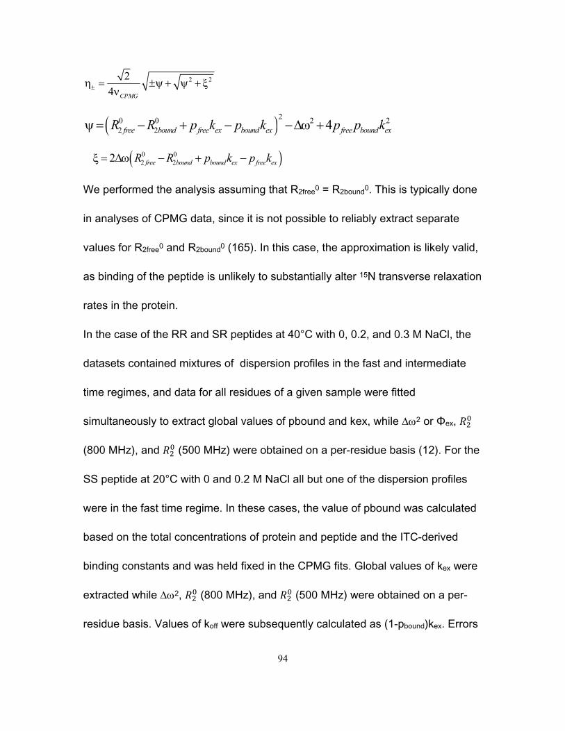
94
2 22
4 CPMG
20 0 2 22 2 4free bound free ex bound ex free bound exR R p k p k p p k
0 02 22 free bound bound ex free exR R p k p k
We performed the analysis assuming that R2free0 = R2bound0. This is typically done
in analyses of CPMG data, since it is not possible to reliably extract separate
values for R2free0 and R2bound0 (165). In this case, the approximation is likely valid,
as binding of the peptide is unlikely to substantially alter 15N transverse relaxation
rates in the protein.
In the case of the RR and SR peptides at 40°C with 0, 0.2, and 0.3 M NaCl, the
datasets contained mixtures of dispersion profiles in the fast and intermediate
time regimes, and data for all residues of a given sample were fitted
simultaneously to extract global values of pbound and kex, while 2 or Φex,
(800 MHz), and (500 MHz) were obtained on a per-residue basis (12). For the
SS peptide at 20°C with 0 and 0.2 M NaCl all but one of the dispersion profiles
were in the fast time regime. In these cases, the value of pbound was calculated
based on the total concentrations of protein and peptide and the ITC-derived
binding constants and was held fixed in the CPMG fits. Global values of kex were
extracted while 2, (800 MHz), and (500 MHz) were obtained on a per-
residue basis. Values of koff were subsequently calculated as (1-pbound)kex. Errors
95
in the extracted parameters were estimated using a Monte Carlo approach in
which group fitting was performed on random subsets of the residues selected
using a bootstrap procedure (166). Analyses were performed using scripts
written in MATLAB (MALAB R2011b, The MathWorks, Natick, MA).
3.3.3. Electrostatic Enhancements
Log10(KA) values for the SS peptide were fitted as a linear function of ionic
strength. Interpolated values were used to calculate the affinity enhancements of
the SR and RR peptides. The corresponding linear interpolation was also used to
calculate kon enhancements. The ionic strength enhancements were plotted as a
function of fion, Equation (3.8), setting r=4Å, which roughly corresponds to the
size scale of a single Arg residue. The plot was not highly sensitive to the choice
of r.
3.3.4. Stopped-flow binding kinetics
The kinetics of binding were characterized by rapidly mixing the SH3 domain and
peptide and monitoring the progress of the reaction via intrinsic tryptophan
fluorescence of the protein, which increases upon interacting with proline-rich
peptides (167). We used a version of the RR peptide free of Trp and Tyr
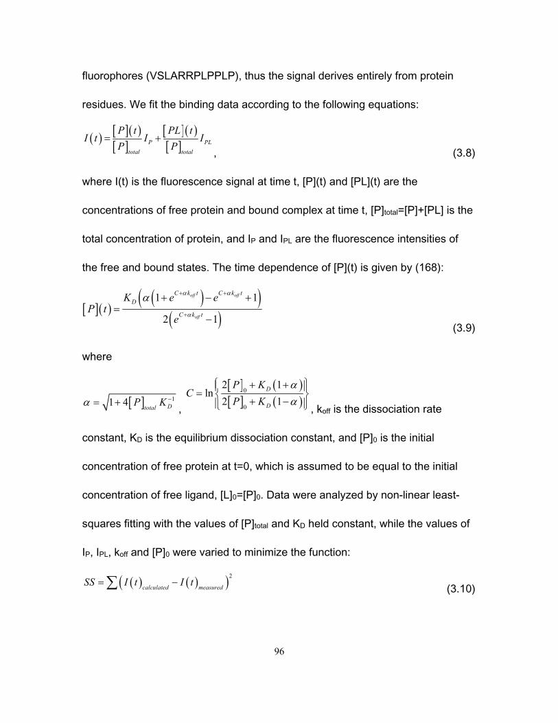
96
fluorophores (VSLARRPLPPLP), thus the signal derives entirely from protein
residues. We fit the binding data according to the following equations:
P PL
total total
P t PL tI t I I
P P
, (3.8)
where I(t) is the fluorescence signal at time t, [P](t) and [PL](t) are the
concentrations of free protein and bound complex at time t, [P]total=[P]+[PL] is the
total concentration of protein, and IP and IPL are the fluorescence intensities of
the free and bound states. The time dependence of [P](t) is given by (168):
1 1
2 1
off off
off
C k t C k t
D
C k t
K e eP t
e
(3.9)
where
11 4 DtotalP K ,
0
0
2 1ln
2 1D
D
P KC
P K
, koff is the dissociation rate
constant, KD is the equilibrium dissociation constant, and [P]0 is the initial
concentration of free protein at t=0, which is assumed to be equal to the initial
concentration of free ligand, [L]0=[P]0. Data were analyzed by non-linear least-
squares fitting with the values of [P]total and KD held constant, while the values of
IP, IPL, koff and [P]0 were varied to minimize the function:
2
calculated measuredSS I t I t (3.10)
97
where I(t)calculated is given by Equation (3.1) and the sum runs over all data points.
The value of [P]total was obtained from the absorbance of the protein sample at
280 nm (169), the concentration of the peptide was determined by amino acid
analysis (170), and the value of KD was extrapolated from temperature-
dependent ITC data for the Fyn SH3/RR peptide interaction (see below).
Adjusting the value of [P]0 accounts for binding that occurs during the dead time
of the instrument (approximately 4 ms). The uncertainty in koff was obtained by
fitting random sets of the 100 individual stop-flow traces selected according to
the bootstrap method (166) and averaged. The error was taken as the standard
deviation obtained after of 100 iterations.
Experiments were performed using a Bio-Logic SFM 400 instrument coupled to a
MOS-250 spectrometer using Biokine 2.5 software for data acquisition. Intrinsic
tryptophan fluorescence of the Fyn SH3 domain was measured with an excitation
wavelength of 276 nm and a bandwidth of 20 nm. Emission at a wavelength of
320 nm and a bandwidth of 10 nm was recorded for 150 milliseconds (ms) with
measurements taken every 0.02 ms. The detector photomultiplier was operated
at 860 Volts. For each trace, 201 uL of protein (1 uM) and 201 uL of RR peptide
(1uM) were mixed for a total injection volume of 402 uL at a flow of 13.5 mL s-1,
at 5°C.
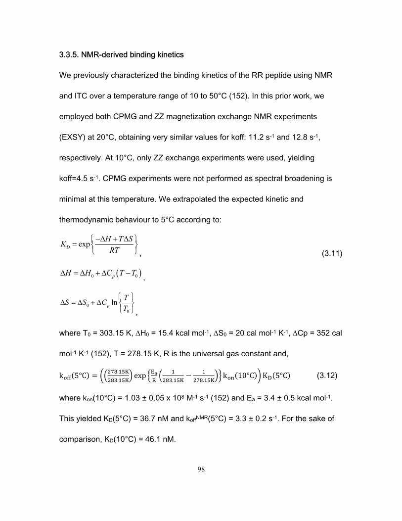
98
3.3.5. NMR-derived binding kinetics
We previously characterized the binding kinetics of the RR peptide using NMR
and ITC over a temperature range of 10 to 50°C (152). In this prior work, we
employed both CPMG and ZZ magnetization exchange NMR experiments
(EXSY) at 20°C, obtaining very similar values for koff: 11.2 s-1 and 12.8 s-1,
respectively. At 10°C, only ZZ exchange experiments were used, yielding
koff=4.5 s-1. CPMG experiments were not performed as spectral broadening is
minimal at this temperature. We extrapolated the expected kinetic and
thermodynamic behaviour to 5°C according to:
expD
H T SK
RT
, (3.11)
0 0pH H C T T ,
00
lnp
TS S C
T
,
where T0 = 303.15 K, H0 = 15.4 kcal mol-1, S0 = 20 cal mol-1 K-1, Cp = 352 cal
mol-1 K-1 (152), T = 278.15 K, R is the universal gas constant and,
k 5°C .
.exp
. .k 10°C K 5°C (3.12)
where kon(10°C) = 1.03 ± 0.05 x 10⁸ M-1 s-1 (152) and Ea = 3.4 ± 0.5 kcal mol-1.
This yielded KD(5°C) = 36.7 nM and koffNMR(5°C) = 3.3 ± 0.2 s-1. For the sake of
comparison, KD(10°C) = 46.1 nM.
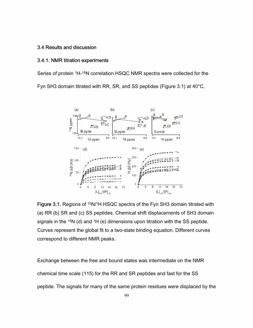
99
3.4 Results and discussion
3.4.1. NMR titration experiments
Series of protein 1H-15N correlation HSQC NMR spectra were collected for the
Fyn SH3 domain titrated with RR, SR, and SS peptides (Figure 3.1) at 40°C.
Figure 3.1. Regions of 15N/1H HSQC spectra of the Fyn SH3 domain titrated with (a) RR (b) SR and (c) SS peptides. Chemical shift displacements of SH3 domain signals in the 15N (d) and 1H (e) dimensions upon titration with the SS peptide. Curves represent the global fit to a two-state binding equation. Different curves correspond to different NMR peaks.
Exchange between the free and bound states was intermediate on the NMR
chemical time scale (115) for the RR and SR peptides and fast for the SS
peptide. The signals for many of the same protein residues were displaced by the
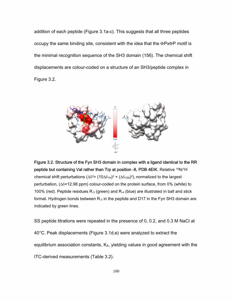
100
addition of each peptide (Figure 3.1a-c). This suggests that all three peptides
occupy the same binding site, consistent with the idea that the PxP motif is
the minimal recognition sequence of the SH3 domain (156). The chemical shift
displacements are colour-coded on a structure of an SH3/peptide complex in
Figure 3.2.
Figure 3.2. Structure of the Fyn SH3 domain in complex with a ligand identical to the RR peptide but containing Val rather than Trp at position -8, PDB 4EIK. Relative 15N/1H chemical shift perturbations (2= (101H)2 + (15N)2), normalized to the largest perturbation, (=12.98 ppm) colour-coded on the protein surface, from 0% (white) to 100% (red). Peptide residues R-3 (green) and R-4 (blue) are illustrated in ball and stick format. Hydrogen bonds between R-3 in the peptide and D17 in the Fyn SH3 domain are indicated by green lines.
SS peptide titrations were repeated in the presence of 0, 0.2, and 0.3 M NaCl at
40°C. Peak displacements (Figure 3.1d,e) were analyzed to extract the
equilibrium association constants, KA, yielding values in good agreement with the
ITC-derived measurements (Table 3.2).
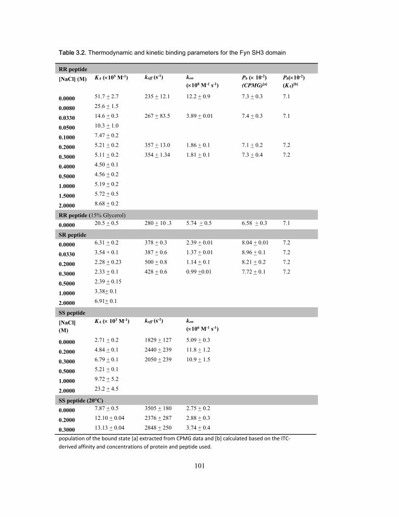
101
Table 3.2. Thermodynamic and kinetic binding parameters for the Fyn SH3 domain
RR peptide
[NaCl] (M) KA (105 M-1) koff (s-1) kon
(108 M-1 s-1) Pb ( 10-2) (CPMG)[a]
Pb(10-2) (KA)[b]
0.0000 51.7 + 2.7 235 + 12.1 12.2 + 0.9 7.3 + 0.3 7.1
0.0080 25.6 + 1.5
0.0330 14.6 + 0.3 267 + 83.5 3.89 + 0.01 7.4 + 0.3 7.1
0.0500 10.3 + 1.0
0.1000 7.47 + 0.2
0.2000 5.21 + 0.2 357 + 13.0 1.86 + 0.1 7.1 + 0.2 7.2
0.3000 5.11 + 0.2 354 + 1.34 1.81 + 0.1 7.3 + 0.4 7.2
0.4000 4.50 + 0.1
0.5000 4.56 + 0.2
1.0000 5.19 + 0.2
1.5000 5.72 + 0.5
2.0000 8.68 + 0.2
RR peptide (15% Glycerol)
0.0000 20.5 + 0.5 280 + 10 .3 5.74 + 0.5 6.58 + 0.3 7.1
SR peptide
0.0000 6.31 + 0.2 378 + 0.3 2.39 + 0.01 8.04 + 0.01 7.2
0.0330 3.54 + 0.1 387 + 0.6 1.37 + 0.01 8.96 + 0.1 7.2
0.2000 2.28 + 0.23 500 + 0.8 1.14 + 0.1 8.21 + 0.2 7.2
0.3000 2.33 + 0.1 428 + 0.6 0.99 +0.01 7.72 + 0.1 7.2
0.5000 2.39 + 0.15
1.0000 3.38+ 0.1
2.0000 6.91+ 0.1
SS peptide
[NaCl] (M)
KA ( 103 M-1) koff (s-1) kon
(106 M-1 s-1)
0.0000 2.71 + 0.2 1829 + 127 5.09 + 0.3
0.2000 4.84 + 0.1 2440 + 239 11.8 + 1.2
0.3000 6.79 + 0.1 2050 + 239 10.9 + 1.5
0.5000 5.21 + 0.1
1.0000 9.72 + 5.2
2.0000 23.2 + 4.5
SS peptide (20°C)
0.0000 7.87 + 0.5 3505 + 180 2.75 + 0.2
0.2000 12.10 + 0.04 2376 + 287 2.88 + 0.3
0.3000 13.13 + 0.04 2848 + 250 3.74 + 0.4
population of the bound state [a] extracted from CPMG data and [b] calculated based on the ITC‐
derived affinity and concentrations of protein and peptide used.
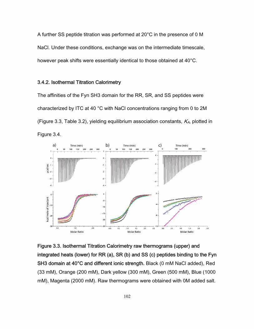
102
A further SS peptide titration was performed at 20°C in the presence of 0 M
NaCl. Under these conditions, exchange was on the intermediate timescale,
however peak shifts were essentially identical to those obtained at 40°C.
3.4.2. Isothermal Titration Calorimetry
The affinities of the Fyn SH3 domain for the RR, SR, and SS peptides were
characterized by ITC at 40 °C with NaCl concentrations ranging from 0 to 2M
(Figure 3.3, Table 3.2), yielding equilibrium association constants, KA, plotted in
Figure 3.4.
Figure 3.3. Isothermal Titration Calorimetry raw thermograms (upper) and integrated heats (lower) for RR (a), SR (b) and SS (c) peptides binding to the Fyn SH3 domain at 40°C and different ionic strength. Black (0 mM NaCl added), Red (33 mM), Orange (200 mM), Dark yellow (300 mM), Green (500 mM), Blue (1000 mM), Magenta (2000 mM). Raw thermograms were obtained with 0M added salt.
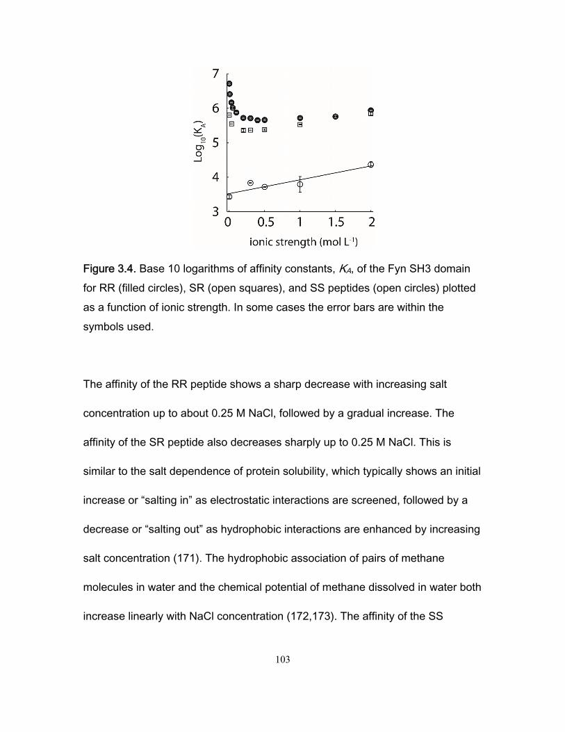
103
Figure 3.4. Base 10 logarithms of affinity constants, KA, of the Fyn SH3 domain for RR (filled circles), SR (open squares), and SS peptides (open circles) plotted as a function of ionic strength. In some cases the error bars are within the symbols used.
The affinity of the RR peptide shows a sharp decrease with increasing salt
concentration up to about 0.25 M NaCl, followed by a gradual increase. The
affinity of the SR peptide also decreases sharply up to 0.25 M NaCl. This is
similar to the salt dependence of protein solubility, which typically shows an initial
increase or “salting in” as electrostatic interactions are screened, followed by a
decrease or “salting out” as hydrophobic interactions are enhanced by increasing
salt concentration (171). The hydrophobic association of pairs of methane
molecules in water and the chemical potential of methane dissolved in water both
increase linearly with NaCl concentration (172,173). The affinity of the SS
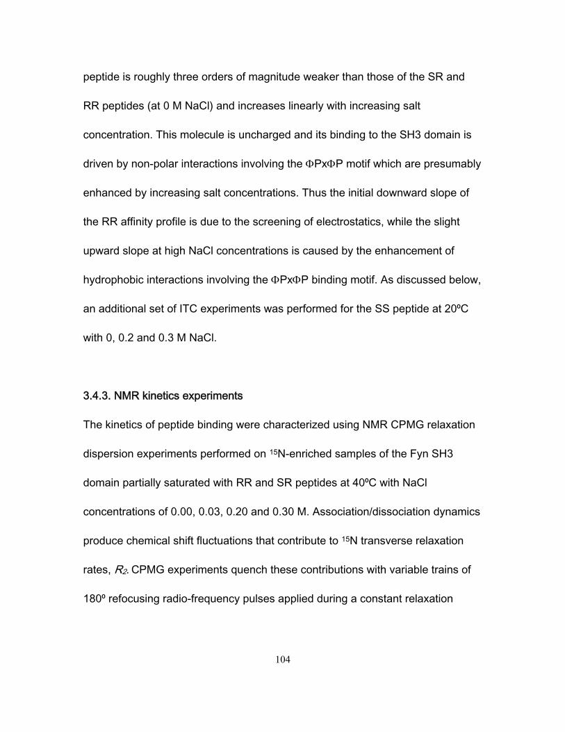
104
peptide is roughly three orders of magnitude weaker than those of the SR and
RR peptides (at 0 M NaCl) and increases linearly with increasing salt
concentration. This molecule is uncharged and its binding to the SH3 domain is
driven by non-polar interactions involving the PxP motif which are presumably
enhanced by increasing salt concentrations. Thus the initial downward slope of
the RR affinity profile is due to the screening of electrostatics, while the slight
upward slope at high NaCl concentrations is caused by the enhancement of
hydrophobic interactions involving the PxP binding motif. As discussed below,
an additional set of ITC experiments was performed for the SS peptide at 20⁰C
with 0, 0.2 and 0.3 M NaCl.
3.4.3. NMR kinetics experiments
The kinetics of peptide binding were characterized using NMR CPMG relaxation
dispersion experiments performed on 15N-enriched samples of the Fyn SH3
domain partially saturated with RR and SR peptides at 40⁰C with NaCl
concentrations of 0.00, 0.03, 0.20 and 0.30 M. Association/dissociation dynamics
produce chemical shift fluctuations that contribute to 15N transverse relaxation
rates, R2. CPMG experiments quench these contributions with variable trains of
180⁰ refocusing radio-frequency pulses applied during a constant relaxation
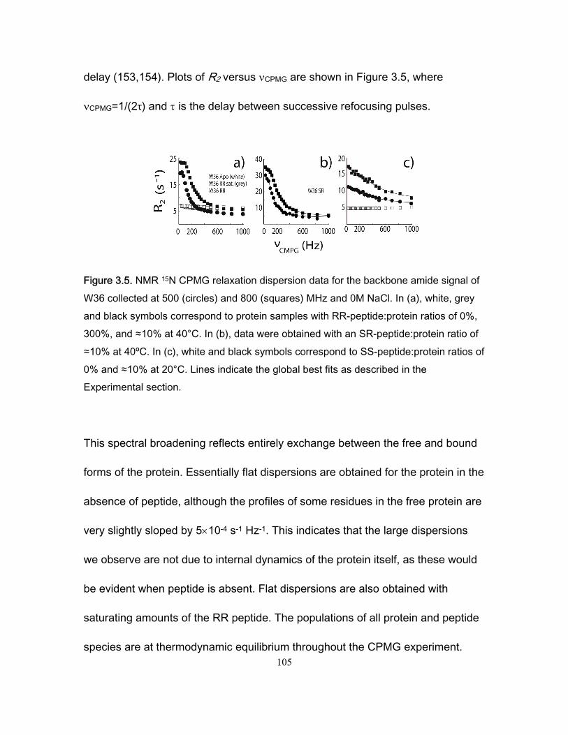
105
delay (153,154). Plots of R2 versus CPMG are shown in Figure 3.5, where
CPMG=1/(2τ) and is the delay between successive refocusing pulses.
Figure 3.5. NMR 15N CPMG relaxation dispersion data for the backbone amide signal of W36 collected at 500 (circles) and 800 (squares) MHz and 0M NaCl. In (a), white, grey and black symbols correspond to protein samples with RR-peptide:protein ratios of 0%, 300%, and ≈10% at 40°C. In (b), data were obtained with an SR-peptide:protein ratio of ≈10% at 40ºC. In (c), white and black symbols correspond to SS-peptide:protein ratios of 0% and ≈10% at 20°C. Lines indicate the global best fits as described in the Experimental section.
This spectral broadening reflects entirely exchange between the free and bound
forms of the protein. Essentially flat dispersions are obtained for the protein in the
absence of peptide, although the profiles of some residues in the free protein are
very slightly sloped by 510-4 s-1 Hz-1. This indicates that the large dispersions
we observe are not due to internal dynamics of the protein itself, as these would
be evident when peptide is absent. Flat dispersions are also obtained with
saturating amounts of the RR peptide. The populations of all protein and peptide
species are at thermodynamic equilibrium throughout the CPMG experiment.
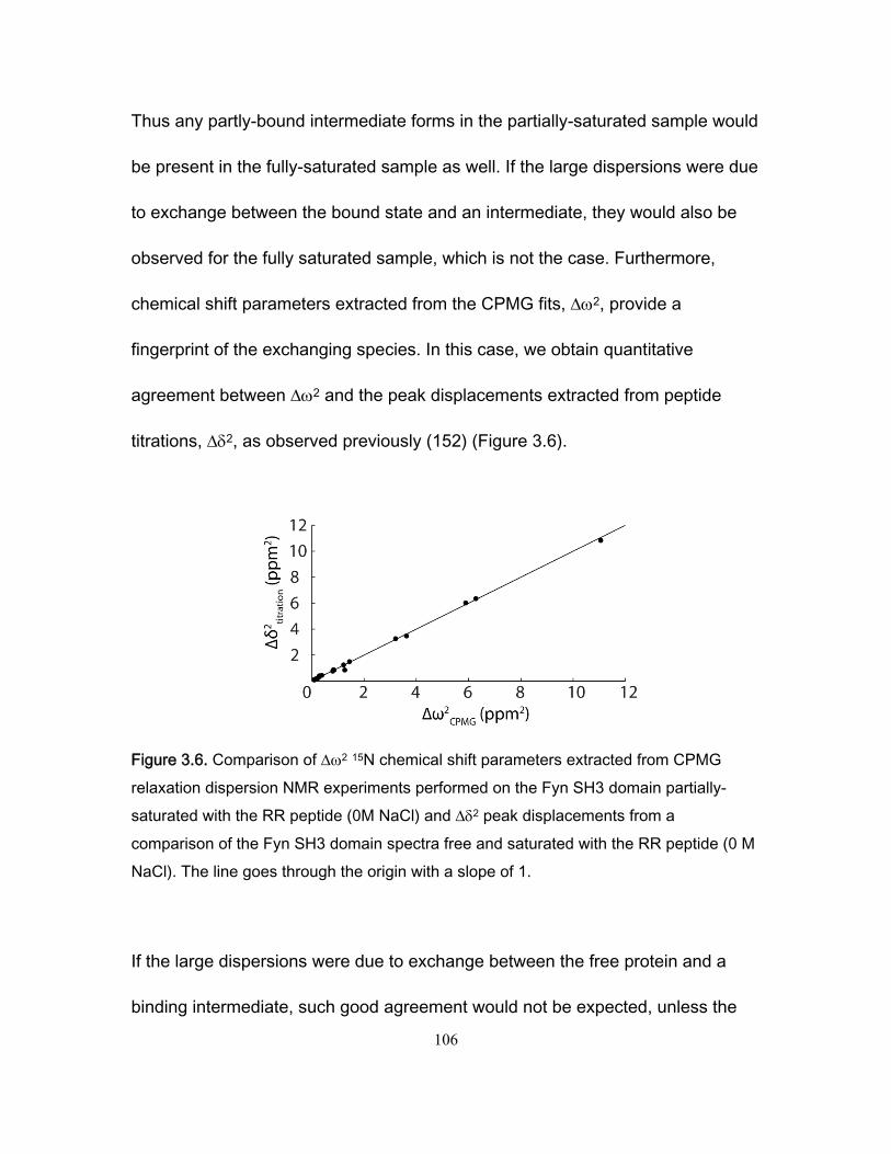
106
Thus any partly-bound intermediate forms in the partially-saturated sample would
be present in the fully-saturated sample as well. If the large dispersions were due
to exchange between the bound state and an intermediate, they would also be
observed for the fully saturated sample, which is not the case. Furthermore,
chemical shift parameters extracted from the CPMG fits, 2, provide a
fingerprint of the exchanging species. In this case, we obtain quantitative
agreement between 2 and the peak displacements extracted from peptide
titrations, 2, as observed previously (152) (Figure 3.6).
Figure 3.6. Comparison of 2 15N chemical shift parameters extracted from CPMG relaxation dispersion NMR experiments performed on the Fyn SH3 domain partially-saturated with the RR peptide (0M NaCl) and 2 peak displacements from a comparison of the Fyn SH3 domain spectra free and saturated with the RR peptide (0 M NaCl). The line goes through the origin with a slope of 1.
If the large dispersions were due to exchange between the free protein and a
binding intermediate, such good agreement would not be expected, unless the
107
intermediate had identical chemical shifts to the bound state, which is unlikely.
Thus the relaxation dispersion analysis reports on the kinetics of exchange
between the free and fully-bound states. Dissociation rate constants, koff, were
extracted from the data as described in the Experimental Section and used to
calculate kon, according to on A offk K k
Experiments with the RR peptide with 0.0 M NaCl were repeated in the presence
of 15% glycerol, which translates into a 1.45-fold increase in solution viscosity,
(174). If binding rates are limited by diffusion in solution then kon should be
inversely proportional to (16), although in practice the slope of a kon/kon0 versus
0/ plot can diverge somewhat from the theoretical value of 1 (175). We find that
the peptide binds 2.13-fold more slowly in the presence of 15% glycerol, which
lies well within the range of viscosity dependences reported for diffusion-limited
protein association rates (175). We also find that the association rate constant is
significantly (approx. 4-fold) more sensitive to ionic strength than the dissociation
rate constant, which is a signature of diffusion-limited binding (130). In addition,
we reported previously that the apparent activation enthalpy (Ea) for kon is 3.4
kcal mol-1 (152). This matches the expected Ea=4.5 kcal mol-1 for diffusion
limited reactions reflecting the temperature dependence of water viscosity (133).
Taken together, the NMR kinetics data strongly indicate that peptide binding to
the SH3 domain is a diffusion-limited, two-state process.
108
In the case of the SS peptide at 40 °C, exchange kinetics are extremely rapid,
leading to very small and essentially linear dispersion profiles. Due to their very
small magnitudes, they are partially obscured by the slightly sloped profiles
obtained for the free protein (which likely reflect some degree of internal motions
unrelated to peptide binding). Therefore in order to determine binding kinetics for
the SS peptide, CPMG experiments were performed at 20⁰C with 0, 0.2, and 0.3
M NaCl, conditions which produce large dispersions for the partially SS peptide-
saturated protein sample, and completely horizontal dispersion profiles for the
free protein, as shown in Figure 5. Values of koff determined at 20⁰C were
combined with affinities, KA, measured by ITC at 20⁰C to yield association rate
constants, kon. We used the previously determined value of Ea=3.4 kcal mol-1 to
extrapolate kon for the SS peptide from 20 to 40°C according to: kon(T2) ≈ (T2/T1)
kon(T1) exp{Ea/R(1/T1- 1/T2)} (176), where R is the gas constant. This leads
to scaling of kon by a factor of only 1.6, which is small compared to the up to 30-
fold differences in kon observed between the different peptides. Thus the results
are not sensitive to the exact choice of Ea.
3.4.4. Comparison of NMR and stopped-flow binding kinetics
In order to cross-validate the NMR characterization of Fyn SH3 domain/peptide
binding kinetics we performed a stopped-flow spectroscopic analysis of the same
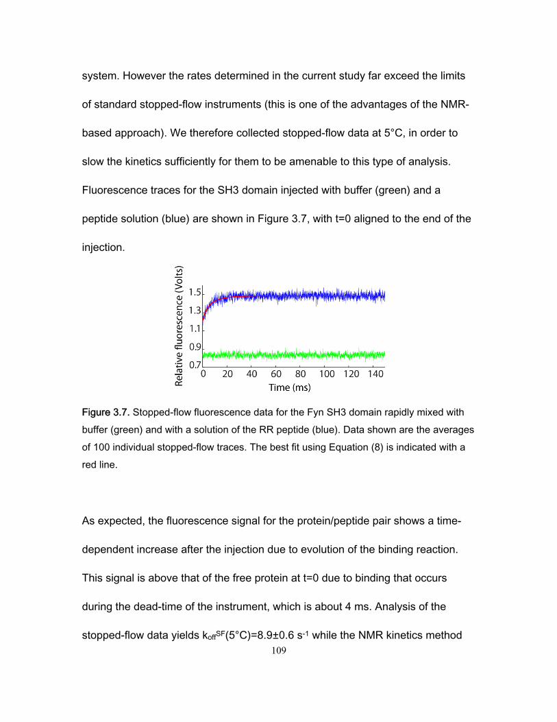
109
system. However the rates determined in the current study far exceed the limits
of standard stopped-flow instruments (this is one of the advantages of the NMR-
based approach). We therefore collected stopped-flow data at 5°C, in order to
slow the kinetics sufficiently for them to be amenable to this type of analysis.
Fluorescence traces for the SH3 domain injected with buffer (green) and a
peptide solution (blue) are shown in Figure 3.7, with t=0 aligned to the end of the
injection.
Figure 3.7. Stopped-flow fluorescence data for the Fyn SH3 domain rapidly mixed with buffer (green) and with a solution of the RR peptide (blue). Data shown are the averages of 100 individual stopped-flow traces. The best fit using Equation (8) is indicated with a red line.
As expected, the fluorescence signal for the protein/peptide pair shows a time-
dependent increase after the injection due to evolution of the binding reaction.
This signal is above that of the free protein at t=0 due to binding that occurs
during the dead-time of the instrument, which is about 4 ms. Analysis of the
stopped-flow data yields koffSF(5°C)=8.9±0.6 s-1 while the NMR kinetics method
110
yields koffNMR(5°C) = 3.3±0.2 s-1, as described in the Methods section. These two
values differ by about a factor of 3, which we believe is excellent agreement for
such different experimental modalities. This gives us further confidence in the
NMR-based kinetics method.
3.4.5. Electrostatic enhancement of association rates
We investigated the influence of electrostatics on SH3 domain ligand binding
kinetics by varying the ionic strength of the samples, in order to attenuate long-
range Coulombic interactions, and by comparing results for the RR, SR, and SS
peptides, which carry formal charges of +2, +1, and 0. The screening of
Coulombic interactions by electrolyte solutions was analyzed in terms of the
electrostatic attraction of two oppositely-charged spheres with radii r, a centre-
centre separation of 2r, and charges ±Z. Relative to infinite separation, the
potential energy, V, is given by the expression (177,178):
2 2
2 ion
Z eV f
r , exp
1ion
rf
r
, (3.13)
e is the elemental charge, is the dielectric constant of the medium, and is the
inverse Debye length,24
B
eI
k T
, kB is the Boltzmann constant and I is the
ionic strength. The parameter fion describes the ionic strength dependence of the
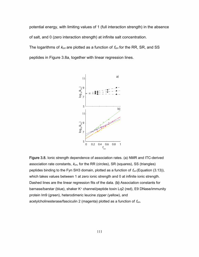
111
potential energy, with limiting values of 1 (full interaction strength) in the absence
of salt, and 0 (zero interaction strength) at infinite salt concentration.
The logarithms of kon are plotted as a function of fion for the RR, SR, and SS
peptides in Figure 3.8a, together with linear regression lines.
Figure 3.8. Ionic strength dependence of association rates. (a) NMR and ITC-derived association rate constants, kon, for the RR (circles), SR (squares), SS (triangles) peptides binding to the Fyn SH3 domain, plotted as a function of fion (Equation (3.13)), which takes values between 1 at zero ionic strength and 0 at infinite ionic strength. Dashed lines are the linear regression fits of the data. (b) Association constants for barnase/barstar (blue), shaker K+ channel/peptide toxin Lq2 (red), E9 DNase/immunity protein Im9 (green), heterodimeric leucine zipper (yellow), and acetylcholinesterase/fasciculin 2 (magenta) plotted as a function of fion.
112
Data for the RR and SR peptides have positive slopes, as expected, since larger
values of fion correspond to lower salt concentrations, greater electrostatic
stabilization of the transition state, and faster association. The data for the SS
peptide are close to horizontal, as expected for an uncharged ligand. The slightly
negative slope may be due to weak hydrophobic stabilization of the transition
state that is enhanced at high salt concentrations. Notably, the lines for the three
peptides nearly intersect at fion=0, and a kon value of about 6107 M-1 s-1. This
corresponds to the basal, or electrostatic-free association rate. The close
agreement of basal association rates obtained for the three different peptides
gives us confidence in the reliability of the extrapolation along fion. The slopes of
the lines correspond to the logarithms of the maximum electrostatic
enhancement of binding with zero ionic strength, log(konenhanced/konbasal). We find
that long-range Coulombic interactions accelerate binding of the RR and SR
peptides by 23.1 and 4.42 fold, respectively, as listed in Table 3.1.
The basal association rate for the SH3 domain is significantly greater, and the
extent of electrostatic enhancement is much less, than observed previously for
long-lived complexes. Association rates for a dataset of five different systems
(130) are plotted as a function of fion in 3.6b and the basal association rates and
electrostatic enhancements extracted from the linear fits are listed in Table 3.1.
These proteins bind roughly 103 to 1010 fold more tightly and dissociate 103 to 109
113
fold more slowly than the SH3 domain studied here. Notably, all of these basal,
electrostatic association rates are 10 to 100 fold slower than those obtained for
the SH3 domain, while the electrostatic rate enhancements are 102 to 104 fold
greater.
It is likely that these differences are due to differences in the nature of the binding
surfaces for the SH3 domain compared to the proteins in long-lived complex
database. The barnase/barstar interface is fairly typical of those in the database
in terms of size and complexity. It buries 1590 Å2 of accessible surface area and
involves the formation of 14 specific hydrogen bonds (179). In this case, only
about 1 molecular collision in 1700 aligns the binding surfaces sufficiently
accurately to proceed to the fully bound state in the absence of electrostatic
enhancement, assuming no charged interactions and a molecular collision
frequency of 6.6 x 10⁹ M-1 s-1 (20). In contrast, the complex formed by the SH3
domain and PxP motif buries only 600 Å2 and is stabilized entirely by
hydrophobic interactions (159). In this case about 1 in every 160 SH3/peptide
collisions is sufficiently well aligned to progress to the bound state. Docking of
the SS peptide onto the SH3 binding surface involves a significantly smaller
contact area with fewer specific pair-wise interactions. This likely results in less
stringent geometric requirements for molecular collisions to lead to successful
docking of the SS peptide and a more rapid basal association rate.
114
A less geometrically restricted transition state could explain our observation of
lower electrostatic enhancement of SH3/peptide association rates compared to
that of barnase/barstar and other long-lived complexes. For barnase/barstar it
was found that the transition state is stabilized by specific charged residues that
are in close proximity in the stereospecific complex. This implies that these
residues are correctly oriented with respect to one another at the rate-limiting
step of binding (124). The SH3 domain exhibits a greater basal association rate,
suggesting that the transition state is less geometrically constrained. Thus fewer
specific interactions may be formed between charged residues in this state,
leading to a smaller degree of electrostatic stabilization.
Thus the SH3 domain and target peptide do not rely as heavily upon electrostatic
enhancement to achieve rapid association kinetics as do many previously-
studied long-lived complexes. It has been previously noted that the interfaces of
high-affinity complexes tend to contain more charged residues than those of low-
affinity ones, and that these Coulombic interactions are sometimes, but not
always, thermodynamically stabilizing (180). This is consistent with higher affinity
complexes relying more heavily on electrostatic enhancement to achieve rapid
binding kinetics than weaker complexes, however the question is far from
resolved.
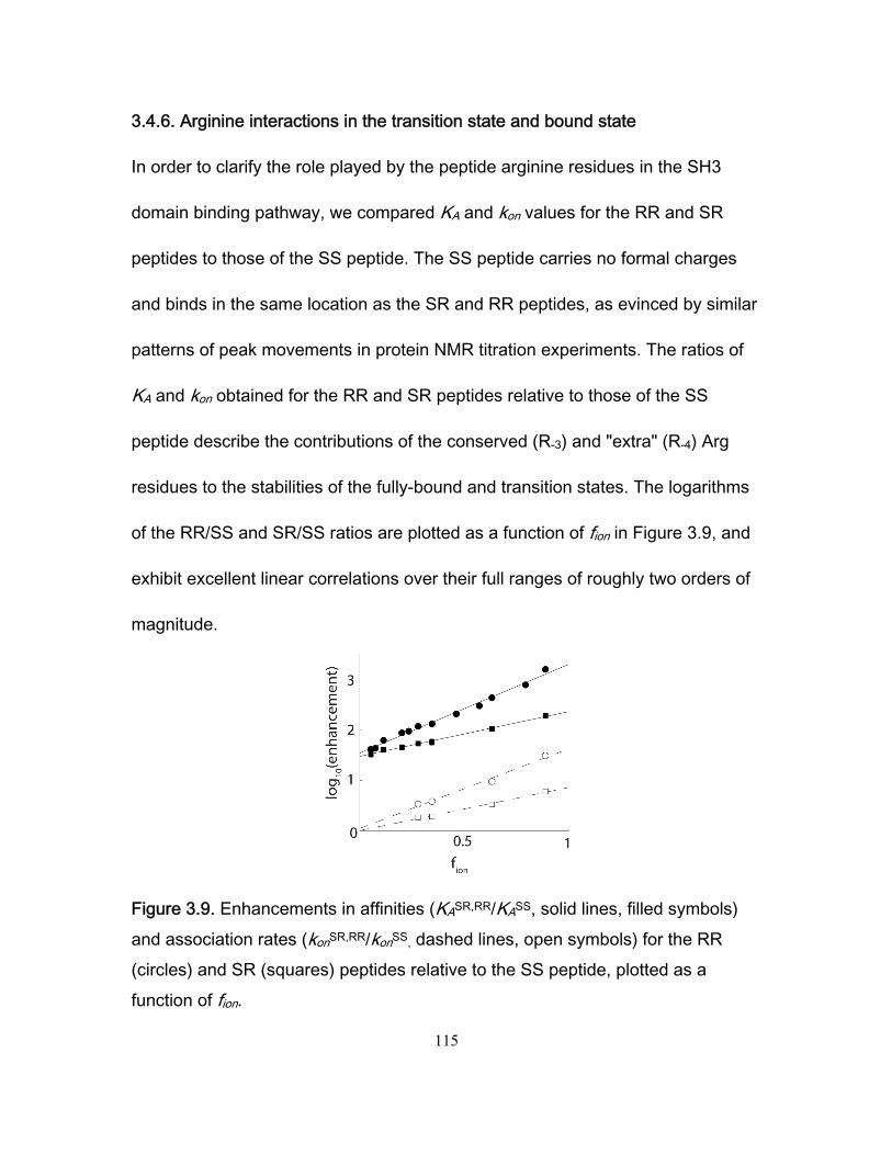
115
3.4.6. Arginine interactions in the transition state and bound state
In order to clarify the role played by the peptide arginine residues in the SH3
domain binding pathway, we compared KA and kon values for the RR and SR
peptides to those of the SS peptide. The SS peptide carries no formal charges
and binds in the same location as the SR and RR peptides, as evinced by similar
patterns of peak movements in protein NMR titration experiments. The ratios of
KA and kon obtained for the RR and SR peptides relative to those of the SS
peptide describe the contributions of the conserved (R-3) and "extra" (R-4) Arg
residues to the stabilities of the fully-bound and transition states. The logarithms
of the RR/SS and SR/SS ratios are plotted as a function of fion in Figure 3.9, and
exhibit excellent linear correlations over their full ranges of roughly two orders of
magnitude.
Figure 3.9. Enhancements in affinities (KASR,RR/KASS, solid lines, filled symbols) and association rates (konSR,RR/konSS, dashed lines, open symbols) for the RR (circles) and SR (squares) peptides relative to the SS peptide, plotted as a function of fion.
116
When extrapolated to infinite salt concentration at the y-intercept, the affinity of
the SR peptide is still enhanced by a factor of 26, relative to the SS peptide,
which translates into a stabilization of the bound state by 2.0 kcal mol-1. This
enhancement is due to interactions formed by R–3 that are not screened by salt
and therefore almost certainly involve short-range forces. The slope for the RR
peptide is greater than that of the SR peptide by about a factor of 2 in Figure 3.9,
consistent with the two-fold difference in formal charge. However, when
extrapolated to infinite salt concentration, the affinities of the two peptides are
virtually identical, as evinced by the intersection of the two lines at the y-axis
(solid lines Figure 3.7). Thus the "extra" R–4 forms long-range electrostatic
interactions in the bound state but no energetically significant short-range (i.e.
unscreened) interactions.
This is consistent with the X-ray crystal structure of the Fyn SH3 domain bound
to a ligand very similar to the RR peptide used in this study (W-8V-8), shown in
Figure 3.2 (159). The conserved R-3 forms a salt bridge (i.e. hydrogen bonds)
with D17, while the aliphatic portion of the residue packs against W36. In
contrast, the "extra" Arg, R–4, points away from D17 and makes no additional
hydrogen bonds. However, negatively-charged E33 and E34 are within about 6.5
Å, well-positioned to interact with R–4 electrostatically. Guanidinium ions,
equivalent to the guanidino moiety of the Arg side-chain, interact with the Fyn
117
SH3 domain specifically at the peptide binding site and compete with the RR
peptide (63). Together, these data strongly suggest that the guanidino moiety of
R–3 interacts with Fyn SH3 domain via a network of hydrogen bonds while R–4
forms looser, long-range electrostatic interactions in the fully-bound complex.
The pattern of enhancements seen for kon is similar, but differs in an important
respect. At 0 M NaCl, the RR peptide binds 5-fold more rapidly than the SR
peptide, which binds 6-fold more rapidly than the SS peptide. This is consistent
with both R–3 and R–4 forming long-range electrostatic interactions in the
transition state. However, in the extrapolation to infinite salt concentration, both
RR and SR peptides bind with rates that are nearly identical to the value
determined for the SS peptide. All of the interactions formed by the peptide Arg
residues in the transition state are thus electrostatic and long-range (i.e. are
screened by salt). The short-range interactions involving R–3 that are present in
the fully-bound complex are only formed after the protein/peptide pair have
passed through the high-energy transition state, i.e. near the end of the binding
process. The transition states of far more tightly-binding partners are believed to
be similarly dominated by long-range electrostatic interactions and lacking in
short-range contacts.(124,131,132,139)
118
3.4.7. Ionic strength dependence of dissociation rates
For diffusion-limited binding reactions, values of kon are typically far more
sensitive to ionic strength than are values of koff.(120,128,140) In the case of the
RR peptide, kon is about 4 times more sensitive to ionic strength than koff. This
has been explained in terms of the structure of the transition state (130). Long-
range electrostatic interactions are fairly insensitive to small changes in charge
separation. Thus if the two binding partners remain close in the transition state,
then long-range electrostatics contribute similarly to the stabilities of the fully-
bound and transition states. Increasing the ionic strength screens the long-range
charge interactions present in both states to equal extents. Thus the barrier to
dissociation is not greatly affected and koff is essentially unchanged. In contrast,
destabilization of the transition state by added salt increases the barrier to
association and slows binding rates.
However this explanation appears inconsistent with mutational analyses of
charge interactions in the fully-bound and transition states. In the case of
barnase/barstar, mutagenesis-derived coupling energies between charged
residues in the fully bound state range from 1-7 kcal mol-1 (159) whereas
coupling energies in the transition state are less than 0.5 kcal mol-1 (124).
Similarly, the SS peptide binds 250-fold more weakly than the SR peptide but
only 6-fold more slowly. The SS peptide binds 1900-fold more weakly and only
119
29-fold more slowly than the RR peptide in the absence of salt. These results
indicate that the interactions of charged residues are much weaker in the
transition state than in the fully-bound state. Adding salt should significantly
destabilize the bound state without significantly affecting the transition state and
thus should increase dissociation rates. Our results provide a simple explanation
for this apparent contradiction. We directly measured electrostatic-free basal
affinities and association rates for the SS peptide, which allowed us to separate
the interaction energies of R-3 and R-4 into long-range “screenable” electrostatic
and short-range “unscreenable” components. Notably, the long-range
components are comparable for the fully-bound and transition states. For the SR
compared to the SS peptide, long-range interactions enhance the affinity and
association rate by factors of 9 and 6, respectively at 0 M NaCl, compared to
250- and 6-fold total enhancements. For the RR peptide, these long-range
enhancement factors are 73 and 29, compared to 1900- and 29-fold total
enhancements. Thus for the Fyn SH3 domain, long-range electrostatic
interactions are similar in the fully-bound and transition states leading to koff
values that are relatively insensitive to ionic strength. This has the implication
that the peptide and SH3 domain are separated by a relatively short distance in
the transition state, as seen previously for long-lived protein complexes (130).
120
3.5. Conclusions
Most of our knowledge of protein binding kinetics derives from studies of
extremely stable long-lived complexes. The binding kinetics of short-lived protein
complexes are less well understood as these systems are challenging to
characterize experimentally. We have applied a recently-developed combination
of NMR and ITC to study complexes of the Fyn SH3 domain and several
peptides whose bound lifetimes are as short as 0.3 ms. This is beyond the range
of standard stopped-flow techniques used to measure binding kinetics. We find
that while the binding pathways of these transient SH3 complexes are similar
those of high-affinity long-lived complexes, they differ in some important
respects.
For the SH3 domain, as well as for high-affinity binding partners, the transition
state is stabilized by long-range electrostatic interactions, while short-range
stereo-specific contacts are formed late in the binding pathway. We find that the
contributions of long-range electrostatic interactions to both the fully-bound and
transition states are quite similar, implying that the separation between the SH3
domain and peptide is not large in the transition state. A similar situation is
believed to hold true for the transition states of high-affinity systems. Thus
structural compactness and the dominance of long-range electrostatic
121
interactions appear to be universal features of diffusion-limited binding pathways
involving affinities and lifetimes spanning up to 7 orders of magnitude.
However, the electrostatic acceleration of SH3 domain association rates is
several orders of magnitude less than has been previously observed for stable
long-lived protein complexes. In contrast, the electrostatic-free basal association
rate is much greater, possibly because of looser geometrical restrictions for
molecular collisions to proceed to the bound state. This raises the interesting
question of whether or not this is a general phenomenon. Do weakly-bound,
transient complexes intrinsically have more rapid basal association rates and
less reliance on electrostatic enhancement than do tightly-bound, long-lived
complexes? If so, how does this relate to the compositions and geometries of the
binding interfaces? The combined NMR and calorimetric approach used here is
uniquely suited for studying transient complexes to gain a better understanding of
the relationships among binding affinities, basal association kinetics, and
electrostatic rate enhancements and to shed light on the fundamental principles
of molecular recognition.
122
3.6. Acknowledgements.
This work was funded by a grant from the Natural Sciences and Engineering
Research Council (NSERC) of Canada. A.M is a member of Groupe de
Recherche Axé sur la Structure des Protéines (GRASP). NMR experiments were
recorded at the Québec/Eastern Canada High Field NMR Facility, supported by
McGill University and GRASP.

123
4. Mapping volume changes in the binding pathway of an SH3 domain and a
proline rich peptide
Research work was done in collaboration with:
Sacha Larda, Pr. Scott Prosser, Department of Chemistry, University of Toronto, UTM. Pressure NMR experiments. Mariano Dellarole, Pr. Catherine A Royer, INSERM U554, Centre de Biochimie Structurale, Montpellier, France. Pressure Fluorescence experiments.
124
4.1. Summary.
Many biological processes involve stereo specific binding of a ligand to a protein.
For this reason, protein-ligand binding pathways is a subject of intense research
in molecular biology. The pathway gives a map that shows how a given
thermodynamic or structural variable influences the stabilities, populations and
formation rates of species during the association process. Numerous theoretical,
computational and experimental studies have been done in order to understand
how temperature, ionic strength, and mutations modulate protein-ligand
association pathways. However, very few studies have characterized changes in
volume occurring during protein-ligand association.
Pressure is perhaps the most convenient tool that can be used to measure
changes in molar volumes in biomolecular processes. Via pressure we can
quantify changes in molar volume for protein-ligand binding (181-187), protein
folding (182,186,188-194) or enzymatic reactions (195,196). In the case of
protein-ligand binding, measuring the association equilibrium constant as a
function of pressure can give the association volume, ΔV. This is the difference in
molar volume between the bound state and the unligated free state. Determining
protein association rate constants at different pressures can also be used to
measure the activation volume, ΔV‡. This is the difference in volume between the
transition state and the free state. These two parameters provide information on
125
the solvation state and the mutual packing of the binding partners through the
association process including the transition state.
We used protein-ligand binding equilibrium experiments that monitored
tryptophan intrinsic fluorescence, together with Nuclear Magnetic Resonance
(NMR) kinetics experiments, to measure the association volume and the
activation volume of binding between chicken tyrosine kinase Fyn SH3 domain
and a proline rich peptide. To our knowledge this is the first measurement of the
activation volume for a protein/ligand binding reaction. We found that the stability
of both the transition state and the final bound complex increased with pressure
compared to the free state. This shows that the molar volume of the transition
state as well as the molar volume of the bound state are lower than the total
volume of the unbound state. These results agree with a protein-ligand binding
pathway that involves significant desolvation of the binding surfaces.
Interestingly, we find that the volume of transition state is very close to that of the
fully bound state. This suggests that the rearrangement of solvating water
molecules and any protein and ligand and conformational changes occur before
the transition state, i.e. before the binding partners cross the energy barrier for
association.
126
4.2. Introduction.
Protein-ligand interactions are essential to living systems. Protein binding
affinities and kinetics are therefore important subjects of study in molecular
biology. Many biologically relevant protein-ligand binding events occur through
fast association processes. However, complexes with very fast association rates
are hard to characterize due to the technical difficulty of measuring fast binding
phenomena. In a typical non-equilibrium binding experiment, binding partners are
quickly mixed and the progress of binding is followed measuring
fluorescence(142,146,197), absorbance(138), suface plasmon resonance(198)
or enzyme activity(120,147,148). In these cases the mixing time must be several
orders of magnitude faster that the association process, otherwise the
association process will be close to the end by the time of the start of the
measurements. NMR dynamics experiments(199) can be effectively used to
address this difficulty. The experiments are usually performed with an isotopically
labeled protein sample containing a substoichiometric amount of the ligand. Due
to the dynamic nature of the binding equilibrium, the NMR signal will lose
intensity and will be broadened. The CPMG experiment applies a series of
refocusing radiofrequency pulses in order to quench the loss of the signal.
Broadening of the NMR signal is then plotted as a function of the frequency of
the refocusing pulses applied. This resulting curve encodes information about the
127
kinetics of binding(200). More precisely, we can extract the dissociation rate
constant, , the relative population of the bound state (pbound) and the
difference in the frequencies of the 15N NMR backbone's amide signals for the
apo and holo states of the protein ∆ . Contrary to stopped flow kinetic
experiments(183), the sample remains at thermodynamic equilibrium avoiding
additional "dead" times required to add or to mix the binding partners. This
makes the maximum association rate limits detectable by NMR much higher than
those that can be measured by other techniques.
In diffusion-limited protein-ligand binding, the association rate is largely
determined by the energy of the transition state, the highest energy point on the
lowest-energy pathway connecting the free and bound states. Many experimental
and theoretical studies have been done in order to describe the transition states
of protein-ligand binding. Many of these studies are based on measuring the
stability of the transition state as a function of temperature(152), ionic
strength(124), directed mutagenesis(140) or through chemical modifications of
the ligand's structure(196). However, to our knowledge, volumetric properties of
protein binding transition states have not been determined. These are of interest
as they are related to conformational changes and rearrangement of solvation
shell. NMR dynamics experiments are ideally suited for this type of analysis since
128
commercially available high-pressure NMR systems can accurately vary the
pressure in the NMR tube with a range of several kilobar.
Pressure is related to volumetric changes occurring during the binding pathway
according to the pressure derivative of the free energy: ∆ ∆ . From this,
it can be derived that ∆
. A plot of vs should
yield a straight line with a slope equal to the molar association volume, ∆ ,
provided that the compressibility of the system is constant within the
experimental pressure range. Similarly, according to the transition state theory,
we can write: ∆ ‡∆ ‡ where G‡ and V‡ are the differences in free energy
and volume between the free state and the transition state, respectively. We will
consider the simple two state binding scheme: ⟷ , where the protein
exchanges between the free state, P, and the final bound conformation PL. From
this model it can be inferred that a plot of RTLn vs p will have as slope
the change in volume between the bound state and the transition state ∆ → ‡.
Using this value and the association volume ∆ , we can calculate ∆ ‡ ∆
∆ → ‡, the activation volume for binding.
Volumetric changes can be related to changes in the molecular structure and
solvation state occurring during binding according to a simple model(201) in
which the association volume is: ∆ ∆ ∆ ∆ ; Where ∆ is the
129
change in the molecular volume. This quantity can be calculated by subtracting
the molecular volumes measured from crystal structures for the free (V and
bound states V , to obtain: ∆ V V ; ∆ measures the change in
volume due to changes in solvation. This term accounts for changes in solvent
volume due to electrostriction or hydrogen binding, i.e., confinement of solvent
molecules on the solvent exposed surface of the protein or the ligand due to
interactions with polar or charged groups. Finally, ∆ describes changes in
thermal volume. is a temperature dependent volume due to the empty layer
generated by the thermal collision between the molecules of the solvent with
protein and ligand residues that are solvent accessible. This term can be
equivalently expressed as ∆ , where is the thickness of the empty
layer and is the change in the surface accessible to solvent upon binding.
We have used intrinsic fluorescence titration experiments and NMR relaxation
dispersion dynamics experiments performed over pressures ranging from 1 to
2000 bar to map the changes in volume occurring along the binding pathway of
the Fyn SH3 domain and a proline rich peptide Ac-FSLARRPLPPLP-NH2. The
peptide used in our studies is a class I proline rich peptide(202) that adopts a
polyproline II helix conformation(36) upon binding. Its sequence contains two
positively charged consecutive R5 R6 residues preceding a proline rich P7 L8 P9
P10 L11 P12 motif that interacts via electrostatics with three negatively charged
130
acidic residues on protein's binding pocket (PDB 4EIK: E99 D100 D101). Using
tryptophan fluorescence titration experiments, we measured a molar association
volume of ~ 44 ml mol-1 (this value is the slope of the curve shown in figure 4.3).
Analysis of changes in molecular volumes using X-ray crystal structures, together
with the measurement of the change in exposed solvent surfaces for the free and
bound states yielded ∆ 114 ml mol-1 (explained in section 4.5.2.) and ∆ -
394 ml mol-1 (see section 4.5.2), giving ∆ 236 ml mol-1 (section 4.5.2). This
agrees with an increase of the interaction volume due to desolvation caused by
the release of densely packed water around polar and charged groups on the
free protein and the free peptide upon the formation of the final bound complex.
CPMG NMR kinetics experiments showed that the difference in volume between
the transition state and the bound complex is just ~ 4 ml mol-1. This value is in
agreement with typical volume changes for hydrogen bond formation(203). The
similar molar volumes obtained for the fully bound and transition states indicate
that conformational changes and solvent rearrangements responsible for the
molar volume of binding are largely complete before the energy barrier to
binding. This contrasts strongly with previous models of the protein binding
transition states in which the protein ligand are separated by several layers of
solvent. Implications for binding pathways are discussed.
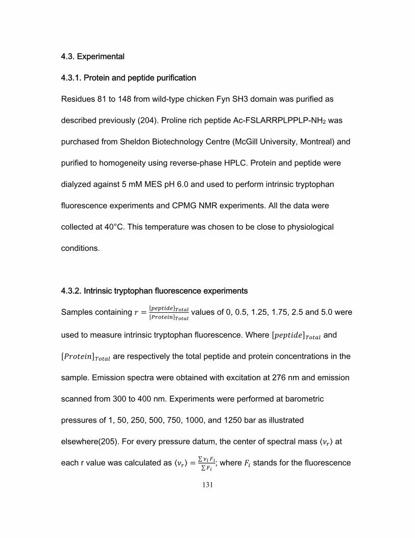
131
4.3. Experimental
4.3.1. Protein and peptide purification
Residues 81 to 148 from wild-type chicken Fyn SH3 domain was purified as
described previously (204). Proline rich peptide Ac-FSLARRPLPPLP-NH2 was
purchased from Sheldon Biotechnology Centre (McGill University, Montreal) and
purified to homogeneity using reverse-phase HPLC. Protein and peptide were
dialyzed against 5 mM MES pH 6.0 and used to perform intrinsic tryptophan
fluorescence experiments and CPMG NMR experiments. All the data were
collected at 40°C. This temperature was chosen to be close to physiological
conditions.
4.3.2. Intrinsic tryptophan fluorescence experiments
Samples containing values of 0, 0.5, 1.25, 1.75, 2.5 and 5.0 were
used to measure intrinsic tryptophan fluorescence. Where and
are respectively the total peptide and protein concentrations in the
sample. Emission spectra were obtained with excitation at 276 nm and emission
scanned from 300 to 400 nm. Experiments were performed at barometric
pressures of 1, 50, 250, 500, 750, 1000, and 1250 bar as illustrated
elsewhere(205). For every pressure datum, the center of spectral mass ⟨ ⟩ at
each r value was calculated as ⟨ ⟩ ∑
∑; where stands for the fluorescence
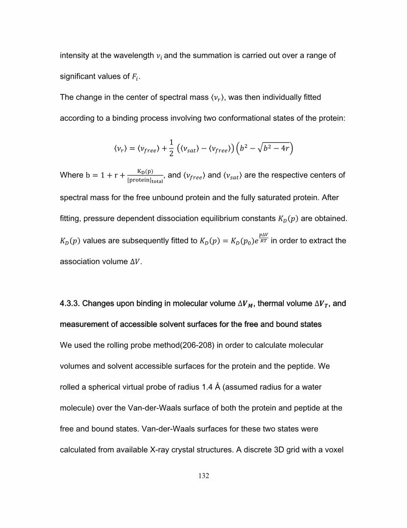
132
intensity at the wavelength and the summation is carried out over a range of
significant values of .
The change in the center of spectral mass ⟨ ⟩, was then individually fitted
according to a binding process involving two conformational states of the protein:
⟨ ⟩ ⟨ ⟩12 ⟨ ⟩ ⟨ ⟩ 4
Where b 1 r , and ⟨ ⟩ and ⟨ ⟩ are the respective centers of
spectral mass for the free unbound protein and the fully saturated protein. After
fitting, pressure dependent dissociation equilibrium constants are obtained.
values are subsequently fitted to ∆
in order to extract the
association volume ∆ .
4.3.3. Changes upon binding in molecular volume ∆ , thermal volume ∆ , and
measurement of accessible solvent surfaces for the free and bound states
We used the rolling probe method(206-208) in order to calculate molecular
volumes and solvent accessible surfaces for the protein and the peptide. We
rolled a spherical virtual probe of radius 1.4 Å (assumed radius for a water
molecule) over the Van-der-Waals surface of both the protein and peptide at the
free and bound states. Van-der-Waals surfaces for these two states were
calculated from available X-ray crystal structures. A discrete 3D grid with a voxel
133
of 0.5 Å was used in all the calculations as described elsewhere(209). PDB entry
3UA6 X-ray crystal structure of the chicken fyn SH3 domain was used to
measure the molecular volume for the free protein V , and also to obtain the
solvent accessible surface of the protein at the free state S . PDB: 4EIK X-ray
crystal structure of the chicken fyn SH3 domain bound to the proline rich peptide
was used to calculate the molecular volume for the final bound state V , and the
solvent accessible surface of the bound complex S . Conformation of the peptide
in the free and bound states were considered to be the same. Upon binding,
proline rich peptide shows a characteristic poly-proline II conformation. It has
been shown that proline rich peptides similar to the one used in our studies can
adopt a poly-proline II conformation in solution at the free state(210). This
particular conformation is also confirmed in the X-ray structure of the bound state
for several types of different proline rich peptides(211). For this reason the Van
der-Waals volume of the peptide at the bound state was used to calculate both
the solvent accessible surface of the free peptide S , and the molecular volume
of the unbound peptide V . Under these conditions we obtain: V V
V and S S S .
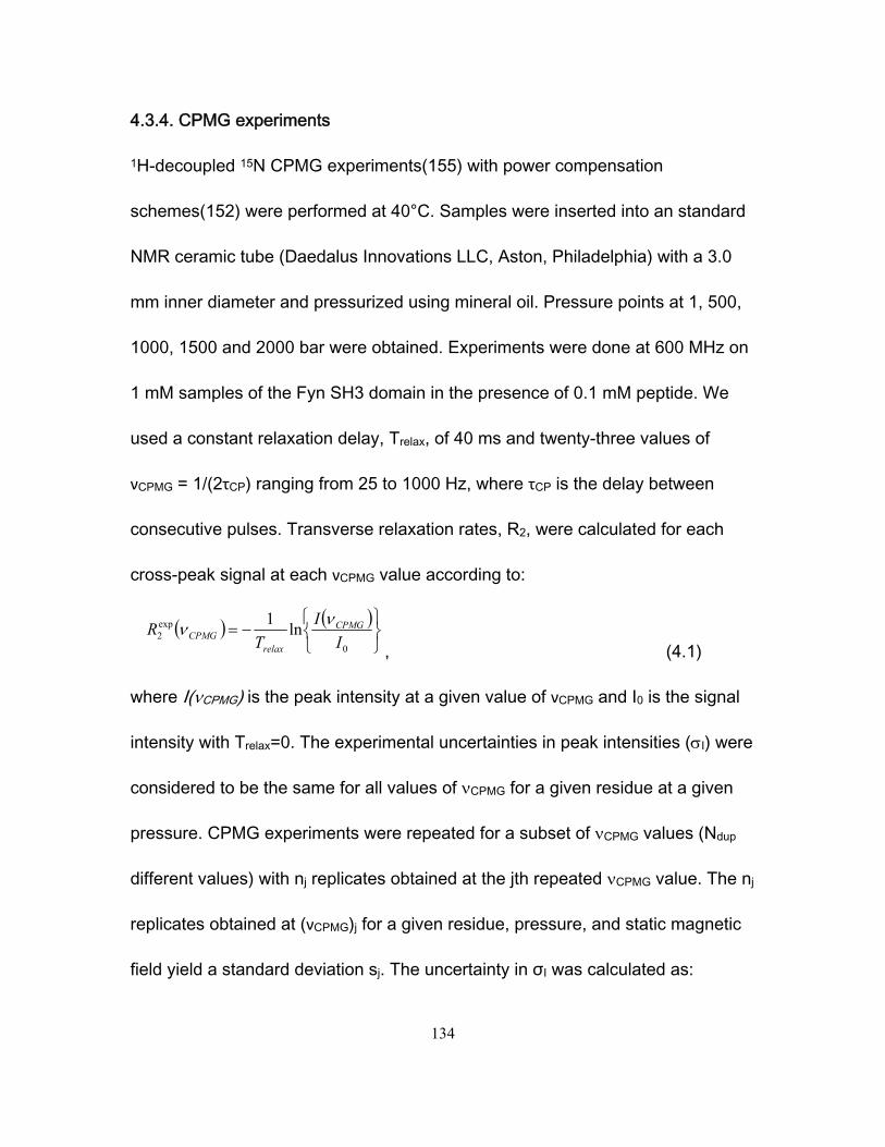
134
4.3.4. CPMG experiments
1H-decoupled 15N CPMG experiments(155) with power compensation
schemes(152) were performed at 40°C. Samples were inserted into an standard
NMR ceramic tube (Daedalus Innovations LLC, Aston, Philadelphia) with a 3.0
mm inner diameter and pressurized using mineral oil. Pressure points at 1, 500,
1000, 1500 and 2000 bar were obtained. Experiments were done at 600 MHz on
1 mM samples of the Fyn SH3 domain in the presence of 0.1 mM peptide. We
used a constant relaxation delay, Trelax, of 40 ms and twenty-three values of
νCPMG = 1/(2τCP) ranging from 25 to 1000 Hz, where τCP is the delay between
consecutive pulses. Transverse relaxation rates, R2, were calculated for each
cross-peak signal at each νCPMG value according to:
0
exp2 ln
1
I
I
TR CPMG
relaxCPMG
, (4.1)
where I(CPMG) is the peak intensity at a given value of νCPMG and I0 is the signal
intensity with Trelax=0. The experimental uncertainties in peak intensities (I) were
considered to be the same for all values of CPMG for a given residue at a given
pressure. CPMG experiments were repeated for a subset of CPMG values (Ndup
different values) with nj replicates obtained at the jth repeated CPMG value. The nj
replicates obtained at (νCPMG)j for a given residue, pressure, and static magnetic
field yield a standard deviation sj. The uncertainty in σI was calculated as:
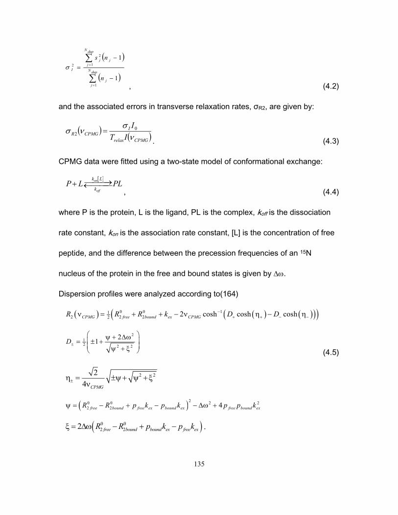
135
dupN
jj
dupN
jjj
I
n
ns
1
1
2
2
1
1
, (4.2)
and the associated errors in transverse relaxation rates, σR2, are given by:
CPMGrelax
ICPMGR IT
I
02
. (4.3)
CPMG data were fitted using a two-state model of conformational exchange:
on
off
k L
kP L PL
, (4.4)
where P is the protein, L is the ligand, PL is the complex, koff is the dissociation
rate constant, kon is the association rate constant, [L] is the concentration of free
peptide, and the difference between the precession frequencies of an 15N
nucleus of the protein in the free and bound states is given by .
Dispersion profiles were analyzed according to(164)
0 0 112 2 22 2 cosh cosh coshCPMG free bound ex CPMGR R R k D D
212 2 2
21D
(4.5)
2 22
4 CPMG
20 0 2 22 2 4free bound free ex bound ex free bound exR R p k p k p p k
0 02 22 free bound bound ex free exR R p k p k .
136
We performed the analysis assuming that R2free0 = R2bound0. This is typically done
in analyses of CPMG data, since it is not possible to reliably extract separate
values for R2free0 and R2bound0.(165) In this case, the approximation is likely valid,
as binding of the peptide is unlikely to substantially alter 15N transverse relaxation
rates in the protein.
Dispersion profiles data for all residues of a given sample were fitted
simultaneously to extract global values of pbound and kex, while 2 or Φex,
R20(600 MHz), were obtained on a per-residue basis.(12) Values of koff were
subsequently calculated as (1-pbound)kex. Errors in the extracted parameters were
estimated using a Monte Carlo approach in which group fitting was performed on
random subsets of the residues selected using a bootstrap procedure.(166)
Analyses were performed using in-house scripts written in MATLAB (MALAB
R2011b, The MathWorks, Natick, MA).
4.5. Results
4.5.1. Intrinsic tryptophan fluorescence experiments
Figure 4.1 shows protein's intrinsic tryptophan fluorescence emission spectra for
chicken fyn SH3 domain containing different concentrations of peptide,
.
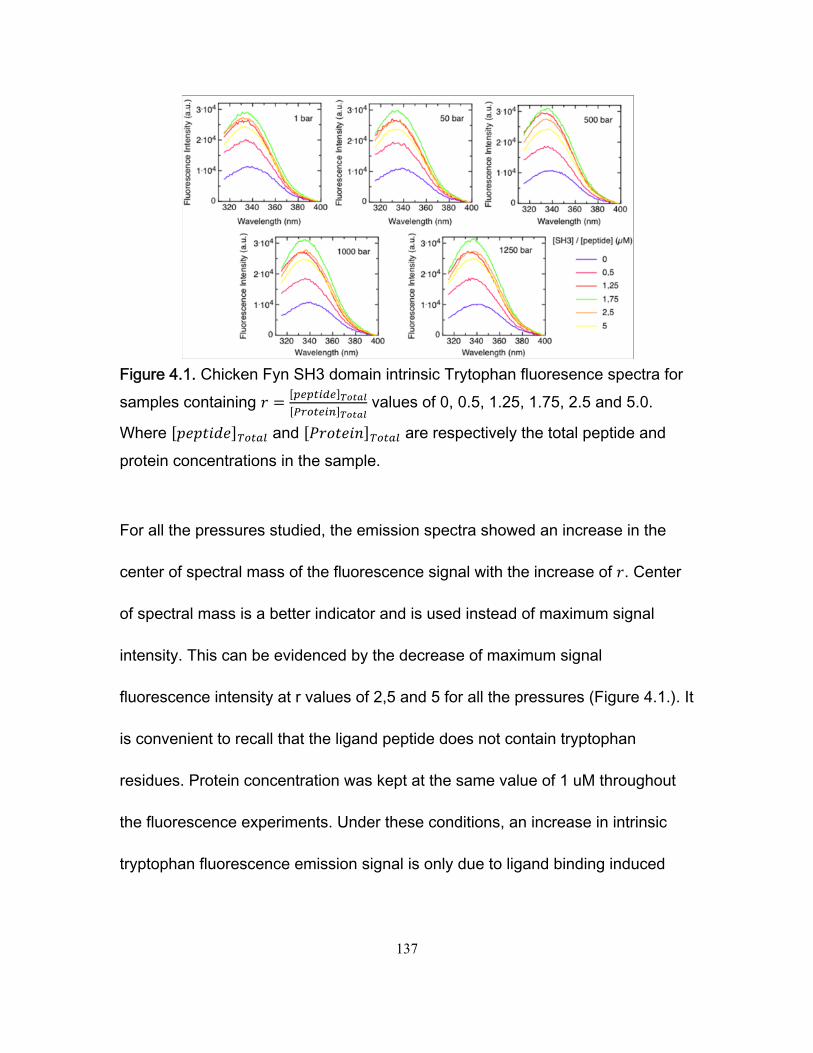
137
Figure 4.1. Chicken Fyn SH3 domain intrinsic Trytophan fluoresence spectra for samples containing values of 0, 0.5, 1.25, 1.75, 2.5 and 5.0.
Where and are respectively the total peptide and protein concentrations in the sample.
For all the pressures studied, the emission spectra showed an increase in the
center of spectral mass of the fluorescence signal with the increase of . Center
of spectral mass is a better indicator and is used instead of maximum signal
intensity. This can be evidenced by the decrease of maximum signal
fluorescence intensity at r values of 2,5 and 5 for all the pressures (Figure 4.1.). It
is convenient to recall that the ligand peptide does not contain tryptophan
residues. Protein concentration was kept at the same value of 1 uM throughout
the fluorescence experiments. Under these conditions, an increase in intrinsic
tryptophan fluorescence emission signal is only due to ligand binding induced
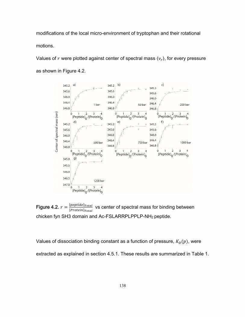
138
modifications of the local micro-environment of tryptophan and their rotational
motions.
Values of were plotted against center of spectral mass ⟨ ⟩, for every pressure
as shown in Figure 4.2.
Figure 4.2. vs center of spectral mass for binding between
chicken fyn SH3 domain and Ac-FSLARRPLPPLP-NH2 peptide.
Values of dissociation binding constant as a function of pressure, , were
extracted as explained in section 4.5.1. These results are summarized in Table 1.
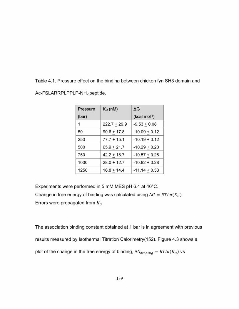
139
Table 4.1. Pressure effect on the binding between chicken fyn SH3 domain and
Ac-FSLARRPLPPLP-NH2 peptide.
Pressure (bar)
KD (nM) ΔG (kcal mol-1)
1 222.7 + 29.9 -9.53 + 0.08
50 90.6 + 17.8 -10.09 + 0.12
250 77.7 + 15.1 -10.19 + 0.12
500 65.9 + 21.7 -10.29 + 0.20
750 42.2 + 18.7 -10.57 + 0.28
1000 28.0 + 12.7 -10.82 + 0.28
1250 16.8 + 14.4 -11.14 + 0.53
Experiments were performed in 5 mM MES pH 6.4 at 40°C. Change in free energy of binding was calculated using ∆ Errors were propagated from
The association binding constant obtained at 1 bar is in agreement with previous
results measured by Isothermal Titration Calorimetry(152). Figure 4.3 shows a
plot of the change in the free energy of binding, ∆ vs
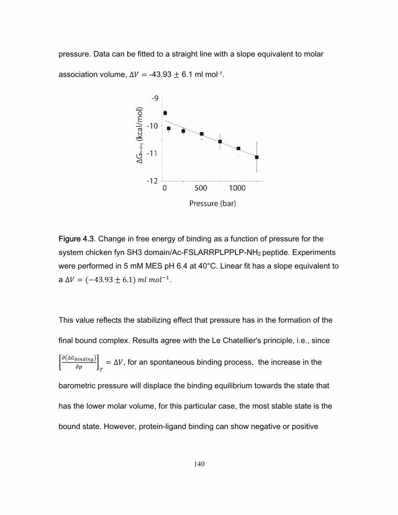
140
pressure. Data can be fitted to a straight line with a slope equivalent to molar
association volume, ∆ -43.93 6.1 ml mol-1.
Figure 4.3. Change in free energy of binding as a function of pressure for the system chicken fyn SH3 domain/Ac-FSLARRPLPPLP-NH2 peptide. Experiments were performed in 5 mM MES pH 6.4 at 40°C. Linear fit has a slope equivalent to a ∆ 43.93 6.1 .
This value reflects the stabilizing effect that pressure has in the formation of the
final bound complex. Results agree with the Le Chatellier's principle, i.e., since
∆∆ , for an spontaneous binding process, the increase in the
barometric pressure will displace the binding equilibrium towards the state that
has the lower molar volume, for this particular case, the most stable state is the
bound state. However, protein-ligand binding can show negative or positive
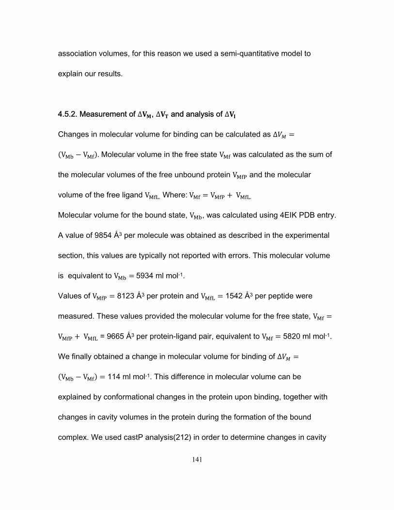
141
association volumes, for this reason we used a semi-quantitative model to
explain our results.
4.5.2. Measurement of ∆ , ∆ and analysis of ∆
Changes in molecular volume for binding can be calculated as ∆
V V . Molecular volume in the free state V was calculated as the sum of
the molecular volumes of the free unbound protein V and the molecular
volume of the free ligand V . Where:V V V .
Molecular volume for the bound state, V , was calculated using 4EIK PDB entry.
A value of 9854 Å3 per molecule was obtained as described in the experimental
section, this values are typically not reported with errors. This molecular volume
is equivalent to V 5934 ml mol-1.
Values of V 8123 Å3 per protein and V 1542 Å3 per peptide were
measured. These values provided the molecular volume for the free state, V
V V = 9665 Å3 per protein-ligand pair, equivalent to V 5820 ml mol-1.
We finally obtained a change in molecular volume for binding of ∆
V V 114 ml mol-1. This difference in molecular volume can be
explained by conformational changes in the protein upon binding, together with
changes in cavity volumes in the protein during the formation of the bound
complex. We used castP analysis(212) in order to determine changes in cavity
142
volumes for both free and bound states of the protein. In crystals obtained at 1
bar we identified a cavity (packing defect), or internal void volume. This cavity
fluctuates among different asymmetric units or crystals as shown in Figure 4.4.
Figure 4.4. Cavity volume calculations for the free and bound states using castP.
The estimated change in volume for that cavity between the free and bound
states is ∆ ~ 38 ml mol-1.This lead us into an scenario where the changes in
molecular volume observed upon binding can be expressed as ∆ ∆
∆ , where ∆ ~76mlmol accounts for the estimated Van der Waals
volume change upon binding(213).
Change in thermal volume was obtained using the expression∆ . A
value of 1 Å for is a good approximation for the effective thickness of the
thermal volume around a globular protein(214). A value for the solvent accessible
143
surface of the bound state S = 3461 Å2 per molecule was obtained. For the free
unbound state we measured the following solvent accessible surfaces: S =
1092 Å2 per peptide molecule, and S = 3023 Å2 per molecule of protein. This
lead us to a change in the solvent accessible surface of S S S = -
654 Å2 per final bound complex formed. This value was used to calculate the
change in thermal volume for the binding process, ∆ 394ml mol-1.
We can use now the expression: ∆ ∆ ∆ ∆ , to estimate the change
in the interaction volume upon binding.We obtained a value of ∆ 236 ml mol-1.
This number is in agreement with similar association process found for several
globular proteins(214). Changes in interaction volumes can also help to estimate
the amount of solvation water molecules surrounding the solvent accessible
surface of the protein in the free unligated state. The value of ∆ can also be
expressed as the product: ∆ ∆ ℎ ℎ , where ℎ and are average
molar volumes for hydration shell water and bulk water, and ∆ ℎ is the number of
hydration water molecules that are released into the bulk solvent upon binding.
An average value for ℎ -1.8 cm3 mol-1 has been already estimated for
globular proteins(214). This reveals a value of ∆ ℎ∆
ℎ131 molecules of
water released per bound complex formed. This value is almost 2 times the
number of the water molecules expected for this protein in the first coordination
water layer. A value of 73 water molecules in the first coordination layer can be
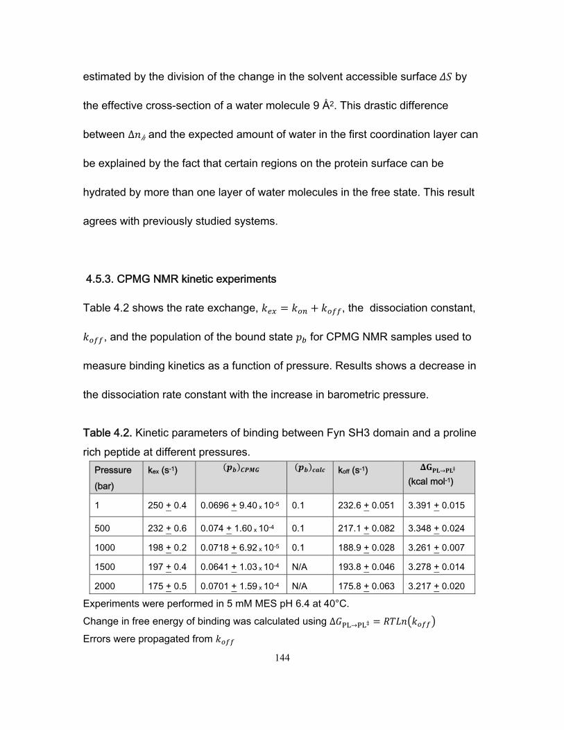
144
estimated by the division of the change in the solvent accessible surface by
the effective cross-section of a water molecule 9 Å2. This drastic difference
between ∆ ℎ and the expected amount of water in the first coordination layer can
be explained by the fact that certain regions on the protein surface can be
hydrated by more than one layer of water molecules in the free state. This result
agrees with previously studied systems.
4.5.3. CPMG NMR kinetic experiments
Table 4.2 shows the rate exchange, , the dissociation constant,
, and the population of the bound state for CPMG NMR samples used to
measure binding kinetics as a function of pressure. Results shows a decrease in
the dissociation rate constant with the increase in barometric pressure.
Table 4.2. Kinetic parameters of binding between Fyn SH3 domain and a proline rich peptide at different pressures.
Pressure (bar)
kex (s-1) koff (s-1) → ‡
(kcal mol-1)
1 250 + 0.4 0.0696 + 9.40 x 10⁻⁵ 0.1 232.6 + 0.051 3.391 + 0.015
500 232 + 0.6 0.074 + 1.60 x 10⁻⁴ 0.1 217.1 + 0.082 3.348 + 0.024
1000 198 + 0.2 0.0718 + 6.92 x 10⁻⁵ 0.1 188.9 + 0.028 3.261 + 0.007
1500 197 + 0.4 0.0641 + 1.03 x 10⁻⁴ N/A 193.8 + 0.046 3.278 + 0.014
2000 175 + 0.5 0.0701 + 1.59 x 10⁻⁴ N/A 175.8 + 0.063 3.217 + 0.020
Experiments were performed in 5 mM MES pH 6.4 at 40°C. Change in free energy of binding was calculated using ∆ → ‡ Errors were propagated from
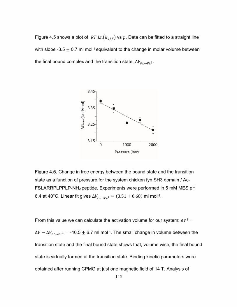
145
Figure 4.5 shows a plot of vs . Data can be fitted to a straight line
with slope -3.5 0.7 ml mol-1 equivalent to the change in molar volume between
the final bound complex and the transition state, ∆ → ‡.
Figure 4.5. Change in free energy between the bound state and the transition state as a function of pressure for the system chicken fyn SH3 domain / Ac-FSLARRPLPPLP-NH2 peptide. Experiments were performed in 5 mM MES pH 6.4 at 40°C. Linear fit gives ∆ → ‡ 3.51 0.68 ml mol-1.
From this value we can calculate the activation volume for our system: ∆ ‡
∆ ∆ → ‡ -40.5 6.7 ml mol-1. The small change in volume between the
transition state and the final bound state shows that, volume wise, the final bound
state is virtually formed at the transition state. Binding kinetic parameters were
obtained after running CPMG at just one magnetic field of 14 T. Analysis of
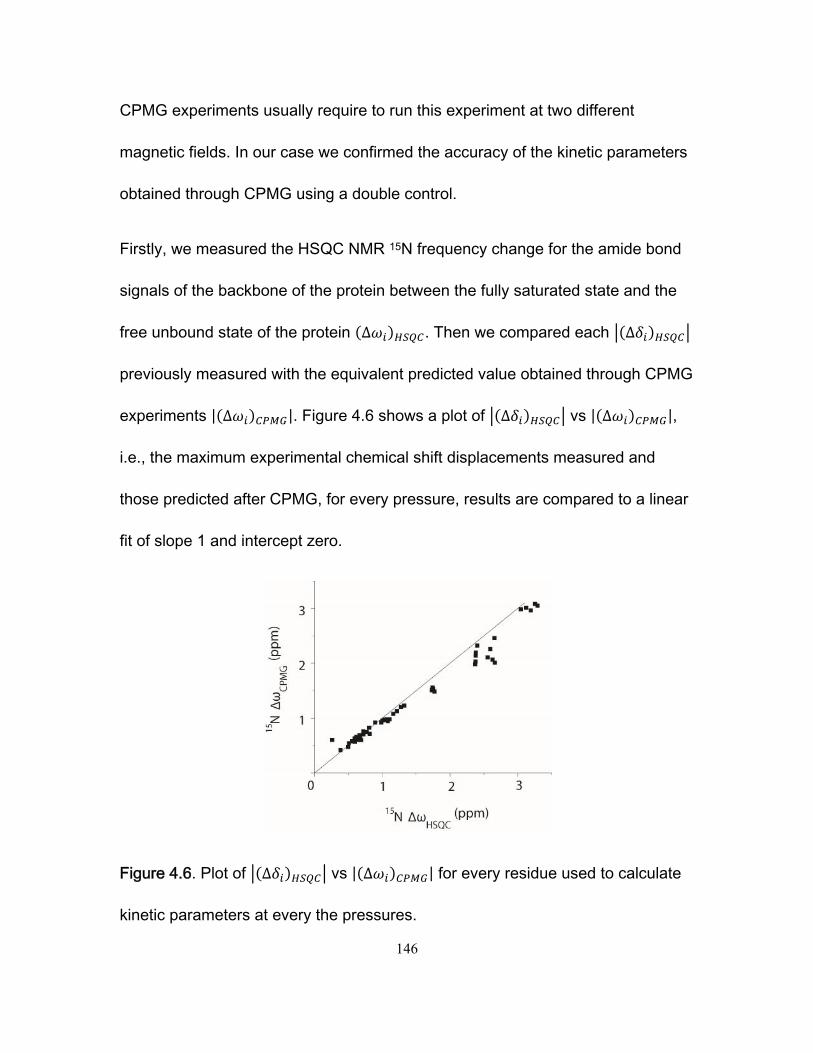
146
CPMG experiments usually require to run this experiment at two different
magnetic fields. In our case we confirmed the accuracy of the kinetic parameters
obtained through CPMG using a double control.
Firstly, we measured the HSQC NMR 15N frequency change for the amide bond
signals of the backbone of the protein between the fully saturated state and the
free unbound state of the protein ∆ . Then we compared each ∆
previously measured with the equivalent predicted value obtained through CPMG
experiments | ∆ |. Figure 4.6 shows a plot of ∆ vs | ∆ |,
i.e., the maximum experimental chemical shift displacements measured and
those predicted after CPMG, for every pressure, results are compared to a linear
fit of slope 1 and intercept zero.
Figure 4.6. Plot of ∆ vs | ∆ | for every residue used to calculate
kinetic parameters at every the pressures.
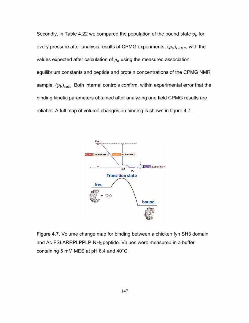
147
Secondly, in Table 4.22 we compared the population of the bound state for
every pressure after analysis results of CPMG experiments, , with the
values expected after calculation of using the measured association
equilibrium constants and peptide and protein concentrations of the CPMG NMR
sample, . Both internal controls confirm, within experimental error that the
binding kinetic parameters obtained after analyzing one field CPMG results are
reliable. A full map of volume changes on binding is shown in figure 4.7.
Figure 4.7. Volume change map for binding between a chicken fyn SH3 domain and Ac-FSLARRPLPPLP-NH2 peptide. Values were measured in a buffer containing 5 mM MES at pH 6.4 and 40°C.
148
4.6 Conclusion
Kinetic NMR methods can be effectively used to measure activation volumes in
fast binding systems. CPMG NMR experiment have proven to be the only
technique available nowadays that can unveil the slight change in volume
between the transition state and the final bound state for binding between
chicken fyn SH3 domain and the peptide Ac-FSLARRPLPPLP-NH2. It was only
through kinetic NMR experiments that we were able to measure the fast,
diffusion limited kinetics of binding of our system.
Results likely show that the binding pathway between the Fyn SH3 domain and
the proline rich peptide goes through a water desolvation step, this desolvation
steps involves more than one coordination water layer for the protein in the free
unbound state. Kinetics NMR experiments also show that the desolvation step is
mostly achieved at the transition state. Results agree with previously studied
systems where the binding stability and the speed of binding is mainly driven by
electrostatics.
149
5. NMR experimental approaches to study binding of bisphophonates to human
Farnesyl Pyrophosphate Synthase (hFPPS)
Research work was done in collaboration with:
Profesor Youla Tsantrizos, Department of Chemistry, McGill University.
150
5.1. Overview.
Farnesyl pyrophosphate synthase (FPPS) is a 1'-4 prenyl transferase, chain
elongation enzyme, that catalyzes two consecutive condensations steps of
isopentenyl diphosphate (IPP) with allylic diphosphates. The first condensation
step is done with dimethylallyl diphosphate (DMAPP) and the second with the
resultant geranyl diphosphate (GPP). The final product of these consecutive
enzymatic reactions is farnesyl pyrophosphate (FPP). FPP is further used in the
synthesis of sterols, dichols, carotenoids, withanolides, ubiquinones,
mitochondrial electron transfer chain components, prenylated proteins and
various sesquiterpenoids including fytoalexins. Isoprenoid biosynthetic pathway
has gained more importance in the last years. This is since key enzymes of this
pathway, including FPPS have been characterized and the their functional roles
in metabolism have been explored using molecular biology.
Human FPPS (hFPPS) is an enzyme with a relevant pharmacological
importance. This synthase is composed of 375 residues and has a molecular
weight over 43 kDa. It plays an important role in the first branching point of the
mevalonate pathway (Figure 5.1).
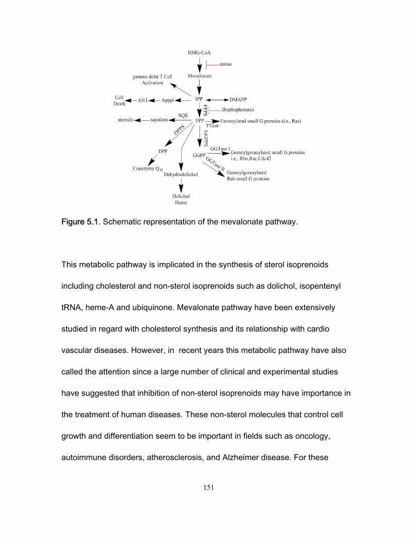
151
Figure 5.1. Schematic representation of the mevalonate pathway.
This metabolic pathway is implicated in the synthesis of sterol isoprenoids
including cholesterol and non-sterol isoprenoids such as dolichol, isopentenyl
tRNA, heme-A and ubiquinone. Mevalonate pathway have been extensively
studied in regard with cholesterol synthesis and its relationship with cardio
vascular diseases. However, in recent years this metabolic pathway have also
called the attention since a large number of clinical and experimental studies
have suggested that inhibition of non-sterol isoprenoids may have importance in
the treatment of human diseases. These non-sterol molecules that control cell
growth and differentiation seem to be important in fields such as oncology,
autoimmune disorders, atherosclerosis, and Alzheimer disease. For these
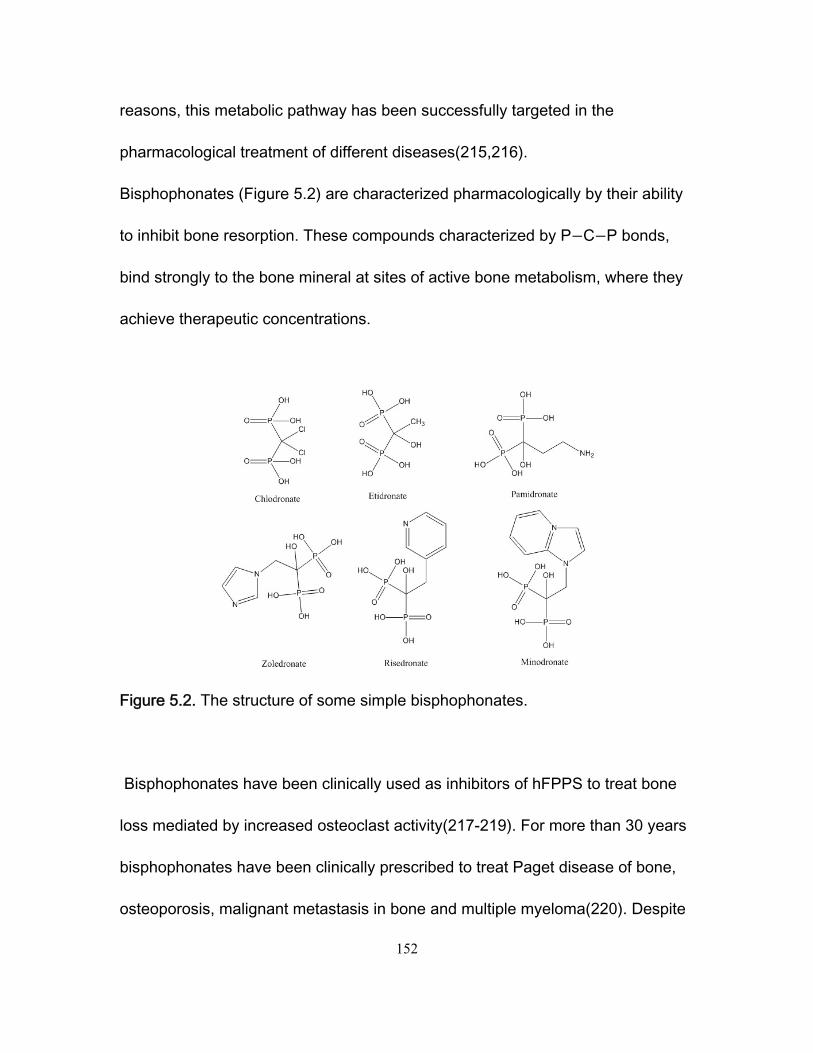
152
reasons, this metabolic pathway has been successfully targeted in the
pharmacological treatment of different diseases(215,216).
Bisphophonates (Figure 5.2) are characterized pharmacologically by their ability
to inhibit bone resorption. These compounds characterized by P C P bonds,
bind strongly to the bone mineral at sites of active bone metabolism, where they
achieve therapeutic concentrations.
Figure 5.2. The structure of some simple bisphophonates.
Bisphophonates have been clinically used as inhibitors of hFPPS to treat bone
loss mediated by increased osteoclast activity(217-219). For more than 30 years
bisphophonates have been clinically prescribed to treat Paget disease of bone,
osteoporosis, malignant metastasis in bone and multiple myeloma(220). Despite
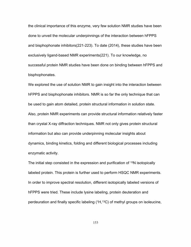
153
the clinical importance of this enzyme, very few solution NMR studies have been
done to unveil the molecular underpinnings of the interaction between hFPPS
and bisphophonate inhibitors(221-223). To date (2014), these studies have been
exclusively ligand-based NMR experiments(221). To our knowledge, no
successful protein NMR studies have been done on binding between hFPPS and
bisphophonates.
We explored the use of solution NMR to gain insight into the interaction between
hFPPS and bisphophonate inhibitors. NMR is so far the only technique that can
be used to gain atom detailed, protein structural information in solution state.
Also, protein NMR experiments can provide structural information relatively faster
than crystal X-ray diffraction techniques. NMR not only gives protein structural
information but also can provide underpinning molecular insights about
dynamics, binding kinetics, folding and different biological processes including
enzymatic activity.
The initial step consisted in the expression and purification of 15N isotopically
labeled protein. This protein is further used to perform HSQC NMR experiments.
In order to improve spectral resolution, different isotopically labeled versions of
hFPPS were tried. These include lysine labeling, protein deuteration and
perdeuration and finally specific labeling (1H,13C) of methyl groups on isoleucine,
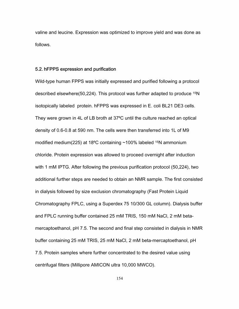
154
valine and leucine. Expression was optimized to improve yield and was done as
follows.
5.2. hFPPS expression and purification
Wild-type human FPPS was initially expressed and purified following a protocol
described elsewhere(50,224). This protocol was further adapted to produce 15N
isotopically labeled protein. hFPPS was expressed in E. coli BL21 DE3 cells.
They were grown in 4L of LB broth at 37⁰C until the culture reached an optical
density of 0.6-0.8 at 590 nm. The cells were then transferred into 1L of M9
modified medium(225) at 18⁰C containing ~100% labeled 15N ammonium
chloride. Protein expression was allowed to proceed overnight after induction
with 1 mM IPTG. After following the previous purification protocol (50,224), two
additional further steps are needed to obtain an NMR sample. The first consisted
in dialysis followed by size exclusion chromatography (Fast Protein Liquid
Chromatography FPLC, using a Superdex 75 10/300 GL column). Dialysis buffer
and FPLC running buffer contained 25 mM TRIS, 150 mM NaCl, 2 mM beta-
mercaptoethanol, pH 7.5. The second and final step consisted in dialysis in NMR
buffer containing 25 mM TRIS, 25 mM NaCl, 2 mM beta-mercaptoethanol, pH
7.5. Protein samples where further concentrated to the desired value using
centrifugal filters (Millipore AMICON ultra 10,000 MWCO).
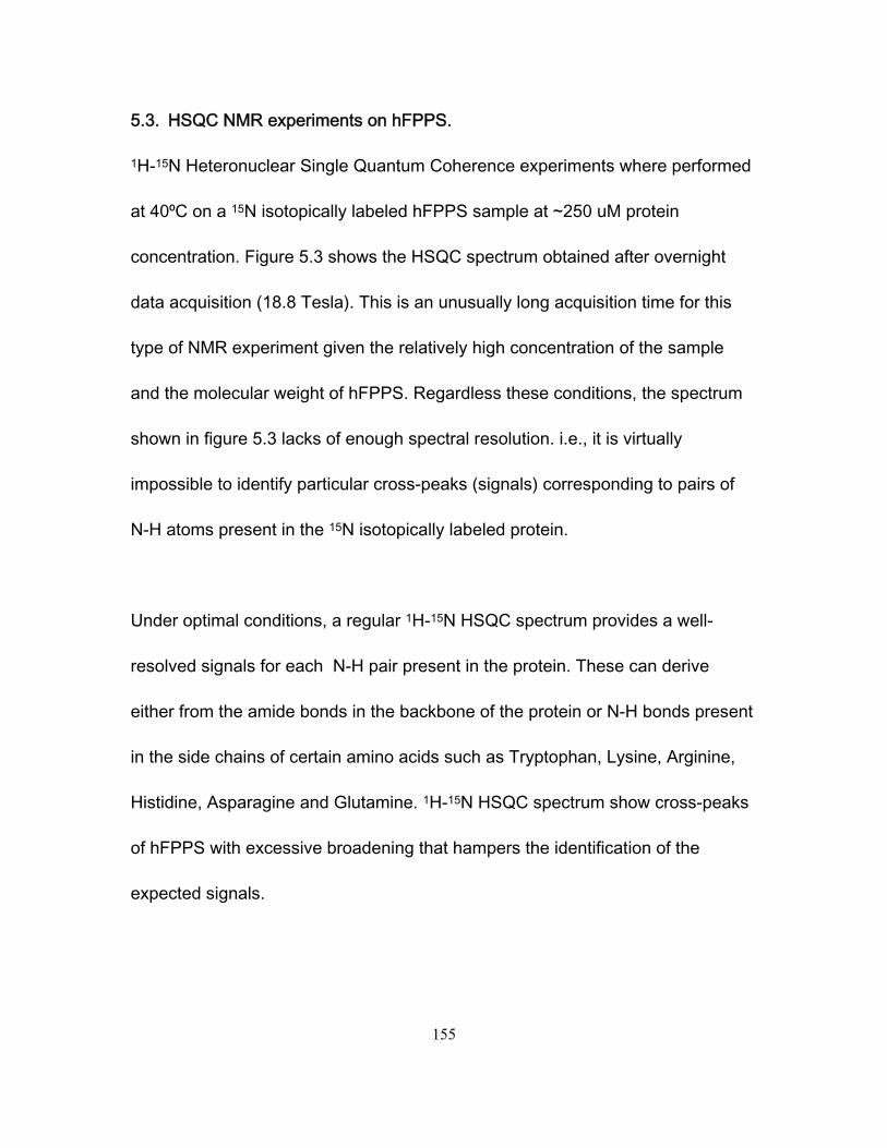
155
5.3. HSQC NMR experiments on hFPPS.
1H-15N Heteronuclear Single Quantum Coherence experiments where performed
at 40⁰C on a 15N isotopically labeled hFPPS sample at ~250 uM protein
concentration. Figure 5.3 shows the HSQC spectrum obtained after overnight
data acquisition (18.8 Tesla). This is an unusually long acquisition time for this
type of NMR experiment given the relatively high concentration of the sample
and the molecular weight of hFPPS. Regardless these conditions, the spectrum
shown in figure 5.3 lacks of enough spectral resolution. i.e., it is virtually
impossible to identify particular cross-peaks (signals) corresponding to pairs of
N-H atoms present in the 15N isotopically labeled protein.
Under optimal conditions, a regular 1H-15N HSQC spectrum provides a well-
resolved signals for each N-H pair present in the protein. These can derive
either from the amide bonds in the backbone of the protein or N-H bonds present
in the side chains of certain amino acids such as Tryptophan, Lysine, Arginine,
Histidine, Asparagine and Glutamine. 1H-15N HSQC spectrum show cross-peaks
of hFPPS with excessive broadening that hampers the identification of the
expected signals.
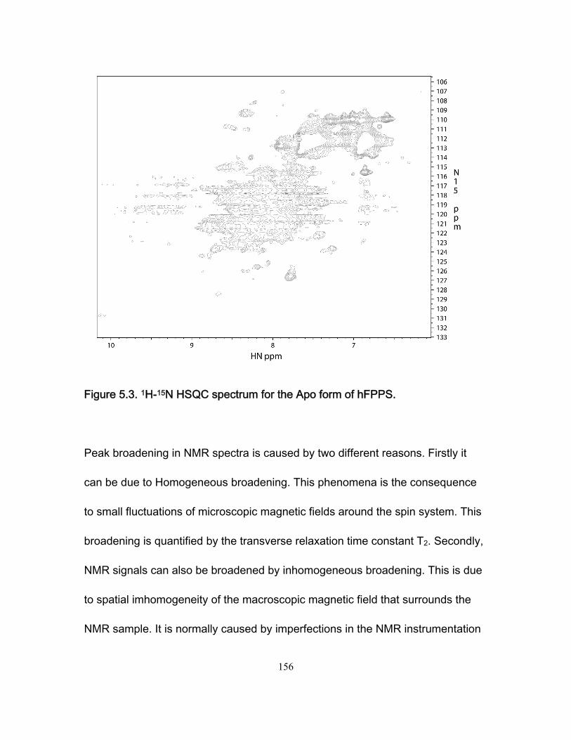
156
Figure 5.3. 1H-15N HSQC spectrum for the Apo form of hFPPS.
Peak broadening in NMR spectra is caused by two different reasons. Firstly it
can be due to Homogeneous broadening. This phenomena is the consequence
to small fluctuations of microscopic magnetic fields around the spin system. This
broadening is quantified by the transverse relaxation time constant T2. Secondly,
NMR signals can also be broadened by inhomogeneous broadening. This is due
to spatial imhomogeneity of the macroscopic magnetic field that surrounds the
NMR sample. It is normally caused by imperfections in the NMR instrumentation
157
or to susceptibility effects in the sample. In order to diminish inhomogeneous
broadening we used Shigemi tubes designed for Varian spectrometers. The next
logical step was to improve NMR spectral resolution by diminishing cross-peak
broadening caused by homogeneous broadening.
Signal broadening observed in the spectrum shown in figure 5.3 may be due to
protein conformational exchange occurring in the millisecond to microsecond
time scale. A protein that can exchange among conformational states in the µs to
ms time scale typically shows NMR signals with broadening or "disappearance"
of certain N-H cross-peaks due to conformational exchange. In order to reduce
exchange, the protein can be locked into a "rigid conformation". i.e., a state
characterized by a relatively slower conformational exchange rate. In this case it
was decided to lock the protein conformation by populating a well characterized
bound state of the enzyme (226,227). According to previous work(50) this can be
achieved by adding to the protein NMR sample a stoichiometric excess of
magnesium, the bisphophonate inhibitor Zoledronate and pyrophosphate. The
final effect of these compounds is to populate a highly stable inhibited state of the
protein. This state reduces the conformational space that hFPPS can populate
and also may decrease the conformational exchange rate of the protein. Figure
5.4 shows the spectrum (18.8 Tesla) of hFPPS (~400 uM) saturated with
158
Magnesium, Zoledronate (~400 uM) and pyrophosphate (~400 uM). Spectral
resolution was improved. However the results obtained are still far from the
quality desired. Under these conditions the system is not suitable to perform any
further binding studies via protein NMR.
Figure 5.4. 1H-15N HSQC for 15N labeled hFPPS saturated with magnesium, the bisphophonate Zoledronate and pyrophosphate.
5.4. Further experiments on hFPPS.
The next objective in this project consisted in increasing signal resolution of NMR
spectra on hFPPS. This was attempted through the implementation of different
159
pulse sequences and also taking advantage of different isotopic labeling
schemes. In either case, the goal was to decrease NMR signal broadening in
order to improve spectral quality.
When a NMR sample is left in a magnetic field for a long time it achieves
"thermal equilibrium". In this state the population of spin systems is governed by
the Bolztmann distribution. Also, at thermal equilibrium, all the components of the
nuclear magnetic moments located in a plane normal (or transverse) to the
applied magnetic field are pointing in random directions. This random distribution
of the magnetic moments implies an absence of nuclear spin coherences. The
concept of coherence can be intuitively grasped by thinking on the idea of
several stopwatches that are started simultaneously at an initial time t0. At a short
period of time after the start, all the clocks will keep registering essentially the
same time, they will maintain synchrony and the stopwatch ensemble will virtually
keep its initial coherence. At a very long time t0+ there will be differences in the
time registered by different stopwatches. This asynchrony is usually due to
stochastic processes and the ensemble of stopwatches have lost its initial
coherence. Something similar happens to the precessing frequencies of nuclear
spins in a sample when certain NMR experiments are performed.
160
These NMR experiments apply radio frequency pulses that manipulate the spin
dynamics of the nuclear magnetic moments in the sample. These pulses usually
redistribute populations of spin systems taking them out of the thermal
equilibrium. In some cases, these pulses can also create coherences. Coherence
is evidenced by a partial alignment of nuclear magnetic moments transverse to
the direction of the external magnetic field applied by the spectrometer.
When the pulse sequence for a particular experiment stops, the nuclear spins are
usually only under the influence of the external magnetic field generated by the
spectrometer's magnet. This makes that the spin system evolves towards a
specific thermal equilibrium via their interaction with the molecular environment.
The process by which this thermal equilibrium is regained is called relaxation.
Relaxation is an important phenomenon in NMR that ultimately defines the
intensity and broadening of the signal measured by most of the NMR
experiments.
In a group of isolated spin 1/2 particles there are two basic time constants to
describe relaxation. The Spin-lattice relaxation time constant, also called
longitudinal relaxation time constant, T1, that measures how fast spin populations
move towards thermal equilibrium, and spin-spin relaxation time constant T2, also
161
known as transverse relaxation time constant, that measures the decay of
transverse magnetization.
In the case of spins 1/2, relaxation is caused by small fluctuations in the
magnetic fields present at the nuclear spins locations. Thermal motion of the
surrounding atoms are the cause of these fluctuations. There are two main
causes of these fluctuations in spins 1/2. One cause is dipole-dipole interactions
(dipole-dipole coupling) between two nuclear spins in the same molecule. In this
case the magnitude and direction of the magnetic field that one spin exerts on
the other constantly changes as the molecule tumbles. Another cause of
fluctuations in the local magnetic fields is chemical shift anisotropy (CSA). These
fluctuating fields are caused by induced molecular electron currents due to the
applied external magnetic field. Tumbling of the molecule changes the magnitude
and direction of the local magnetic fields causing relaxation. There are also
effects in the local fields due to spin-rotation. However, this has a minor effect in
the relaxation mechanisms for spins 1/2. For spins 1/2 the dominant relaxation
mechanism is dipole-dipole interactions, and at higher applied external magnetic
fields, CSA starts to be a competitive cause of relaxation. As the protein tumbles,
the induced fields at certain nucleus are modulated leading to relaxation. This is
the main mechanism of relaxation via CSA. These induced fields are proportional
162
to the spectrometer external applied magnetic field and the relaxation constants
are proportional to the square of the local magnetic fields. As a consequence of
this, The CSA relaxation mechanism is proportional to the square of the external
magnetic field and becomes competitive with the dipole-dipole relaxation
mechanism at the highest comercially available magnetic field (22.3 T). When a
system present several correlated mechanisms of relaxation, there are
possibilities of cross-relaxation effects. Cross-relaxation effects can be
successfully used in some pulse sequences to improve spectral resolution as in
the case of Transverse Relaxation Optimized Spectroscopy experiments
(TROSY)(228).
With the previous information in mind it was decided to keep studying the
interaction between hFPPS and bisphophonates applying different pulse
sequences and using certain isotopic labeling schemes. Both scenarios involved
strategies that were intended to enhance spectral resolution by improving NMR
relaxation properties in the sample.
5.4.1. Lysine methylation of hFPPS.
Fast rotation of methyl groups provide them with long transverse relaxation time
constants. This provides them with favorable NMR relaxation properties. These
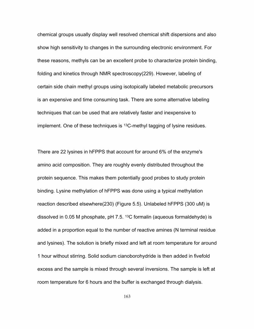
163
chemical groups usually display well resolved chemical shift dispersions and also
show high sensitivity to changes in the surrounding electronic environment. For
these reasons, methyls can be an excellent probe to characterize protein binding,
folding and kinetics through NMR spectroscopy(229). However, labeling of
certain side chain methyl groups using isotopically labeled metabolic precursors
is an expensive and time consuming task. There are some alternative labeling
techniques that can be used that are relatively faster and inexpensive to
implement. One of these techniques is 13C-methyl tagging of lysine residues.
There are 22 lysines in hFPPS that account for around 6% of the enzyme's
amino acid composition. They are roughly evenly distributed throughout the
protein sequence. This makes them potentially good probes to study protein
binding. Lysine methylation of hFPPS was done using a typical methylation
reaction described elsewhere(230) (Figure 5.5). Unlabeled hFPPS (300 uM) is
dissolved in 0.05 M phosphate, pH 7.5. 13C formalin (aqueous formaldehyde) is
added in a proportion equal to the number of reactive amines (N terminal residue
and lysines). The solution is briefly mixed and left at room temperature for around
1 hour without stirring. Solid sodium cianoborohydride is then added in fivefold
excess and the sample is mixed through several inversions. The sample is left at
room temperature for 6 hours and the buffer is exchanged through dialysis.
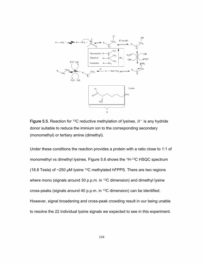
164
Figure 5.5. Reaction for 13C reductive methylation of lysines. is any hydride donor suitable to reduce the iminium ion to the corresponding secondary (monomethyl) or tertiary amine (dimethyl). Under these conditions the reaction provides a protein with a ratio close to 1:1 of
monomethyl vs dimethyl lysines. Figure 5.6 shows the 1H-13C HSQC spectrum
(18.8 Tesla) of ~250 µM lysine 13C methylated hFPPS. There are two regions
where mono (signals around 30 p.p.m. in 13C dimension) and dimethyl lysine
cross-peaks (signals around 40 p.p.m. in 13C dimension) can be identified.
However, signal broadening and cross-peak crowding result in our being unable
to resolve the 22 individual lysine signals we expected to see in this experiment.
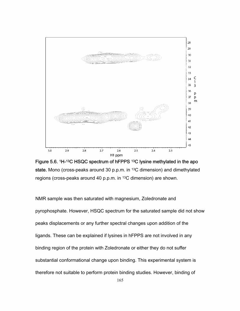
165
Figure 5.6. 1H-13C HSQC spectrum of hFPPS 13C lysine methylated in the apo state. Mono (cross-peaks around 30 p.p.m. in 13C dimension) and dimethylated regions (cross-peaks around 40 p.p.m. in 13C dimension) are shown.
NMR sample was then saturated with magnesium, Zoledronate and
pyrophosphate. However, HSQC spectrum for the saturated sample did not show
peaks displacements or any further spectral changes upon addition of the
ligands. These can be explained if lysines in hFPPS are not involved in any
binding region of the protein with Zoledronate or either they do not suffer
substantial conformational change upon binding. This experimental system is
therefore not suitable to perform protein binding studies. However, binding of
166
wild-type hFPPS to Zoledronate was confirmed by Isothermal titration
calorimetry. Enzymatic activity of the protein was also confirmed by further
assays made by an independent lab partner as illustrated in the literature(223).
5.4.2. hFPPS deuteration.
In addition to CSA, dipole-dipole interactions are the most important cause of
NMR signal relaxation in spin 1/2 systems. A straightforward way to reduce this
specific relaxation is by removing intramolecular dipole-dipole interactions. In our
particular case the protein contains 1H,15N,and 13C, nuclei, which are all spin 1/2
particles. Dipole-dipole interactions, transverse relaxation, and thus sensitivity
can be increased by reducing the number of these spins in our sample. 15N and
13C atoms do not cause much relaxation given their very small gyromagnetic
ratio. However 1H are the most abundand source of relaxation and they can be
sometimes replaced with 2H without disrupting protein function or structure(231).
However not all 1H nuclei are desired to be removed, some few of them can be
kept as NMR reporters in the protein to track protein binding, folding, or any
conformational change of interest. 1H atoms are the main source of spins 1/2 in
proteins. By selectively replacing some 1H atoms with 2H atoms we can
drastically reduce relaxation due to dipole-dipole interactions.
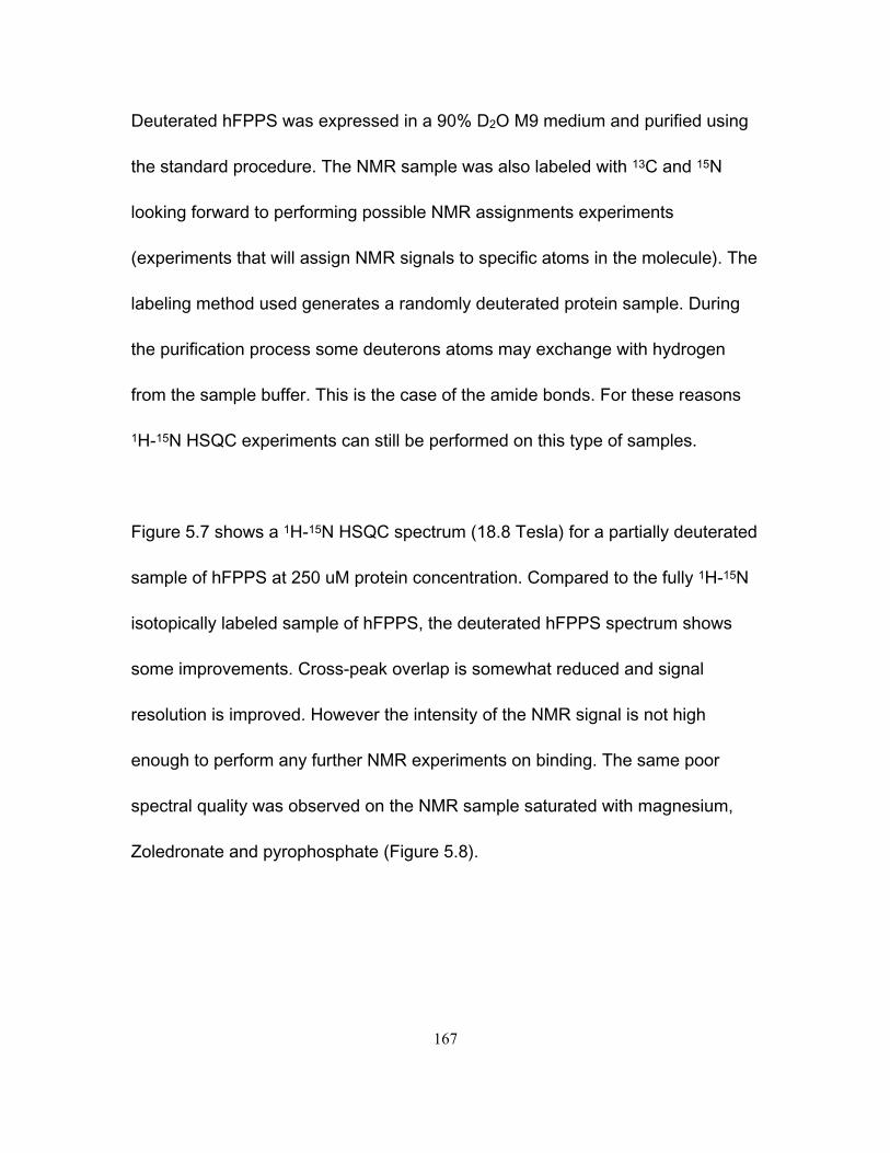
167
Deuterated hFPPS was expressed in a 90% D2O M9 medium and purified using
the standard procedure. The NMR sample was also labeled with 13C and 15N
looking forward to performing possible NMR assignments experiments
(experiments that will assign NMR signals to specific atoms in the molecule). The
labeling method used generates a randomly deuterated protein sample. During
the purification process some deuterons atoms may exchange with hydrogen
from the sample buffer. This is the case of the amide bonds. For these reasons
1H-15N HSQC experiments can still be performed on this type of samples.
Figure 5.7 shows a 1H-15N HSQC spectrum (18.8 Tesla) for a partially deuterated
sample of hFPPS at 250 uM protein concentration. Compared to the fully 1H-15N
isotopically labeled sample of hFPPS, the deuterated hFPPS spectrum shows
some improvements. Cross-peak overlap is somewhat reduced and signal
resolution is improved. However the intensity of the NMR signal is not high
enough to perform any further NMR experiments on binding. The same poor
spectral quality was observed on the NMR sample saturated with magnesium,
Zoledronate and pyrophosphate (Figure 5.8).
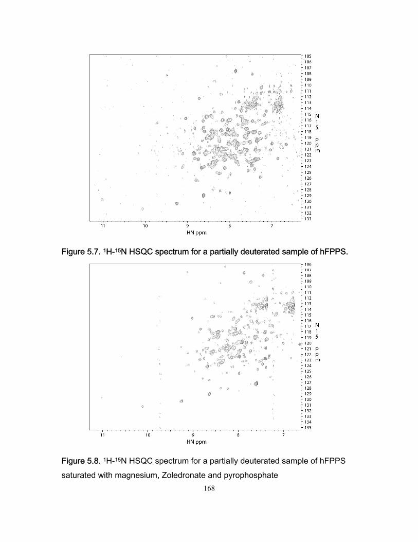
168
Figure 5.7. 1H-15N HSQC spectrum for a partially deuterated sample of hFPPS.
Figure 5.8. 1H-15N HSQC spectrum for a partially deuterated sample of hFPPS saturated with magnesium, Zoledronate and pyrophosphate
169
5.4.3. hFPPS perdeuteration and 1H-13C labeling of methyl groups on
isoleucines, leucines and valines using metabolic precursors
A final step was taken to study the binding of hFPPS to bisphonates using NMR.
This final approach included perdeuteration of the protein, selective 1H-13C
labeling of methyl groups on Isoleucine, leucine and valine using metabolic
precursors and use of NMR experiments that include TROSY pulse sequences.
Perdeuteration implies that every 1H in the protein is replaced by 2H. In order to
do this, every nutrient supplied to the E.coli used to express the protein is fully
deuterated. Protein perdeuteration strategies are extensively used to study large
proteins. Perdeuteration is usually performed concurrently with selective labeling
schemes. In this case, selective methylation of hFPPS was achieved using
specific isotopic labeled precursors (1H,2H,13C) alpha-ketobutyrate and alpha-
ketoisovalarate. The perdeuteration-methyl labeling protocol used here is
described elsewhere(232).
A sample of hFPPS containing protons only on the methyl groups of isoleucine
(only δ1), leucine (13CH3,12C2H3) and valine (13CH3,12C2H3) was expressed, the
enzyme was 15N,13C,2H labeled elsewhere. The protein was further purified using
170
and the standard protocol and many or all amide positions were reprotonated to
obtain a 300 uM protein concentration sample. Figure 5.5 shows an 1H-15N
spectrum TROSY-HSQC experiment (18.8 Tesla) for perdeuterated, methyl
labeled hFPPS in the apo state. A TROSY sequence was run in order to increase
signal resolution. TROSY pulse sequences take advantage of cross relaxation
interplay between spin-spin interactions, and chemical shift anisotropy effects
(preferably at high magnetic fields) The experiment then selects NMR signals
with desirable slower relaxation rates. TROSY-HSQC pulse sequence used in
this experiment is explained elsewhere(228). However, amide cross-peak signals
obtained in the spectrum shown in figure 5.9 lack sufficient spectral resolution for
further NMR assignment experiments.
Figure 5.10 shows a 1H-13C methyl HMQC experiment (18.8 Tesla) for a 300uM
sample of hFPPS in the apo state. This experiment uses TROSY pulse
sequences to detect signals from 1H-13C methyl labeled isoleucines, valines and
isoleucines present in hFPPS. Spectral resolution and cross-peak intensities are
very poor. Ultimately, we were unable to identify individual crosspeaks from
labeled methyls on hFPPS.
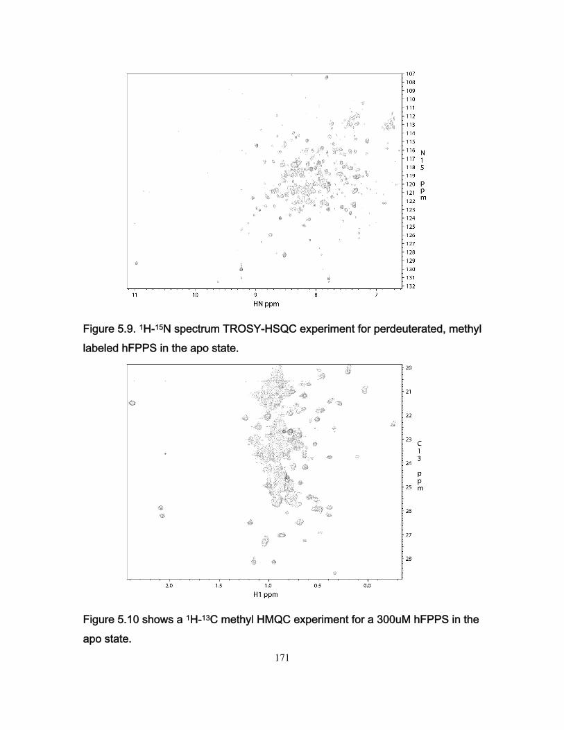
171
Figure 5.9. 1H-15N spectrum TROSY-HSQC experiment for perdeuterated, methyl labeled hFPPS in the apo state.
Figure 5.10 shows a 1H-13C methyl HMQC experiment for a 300uM hFPPS in the apo state.
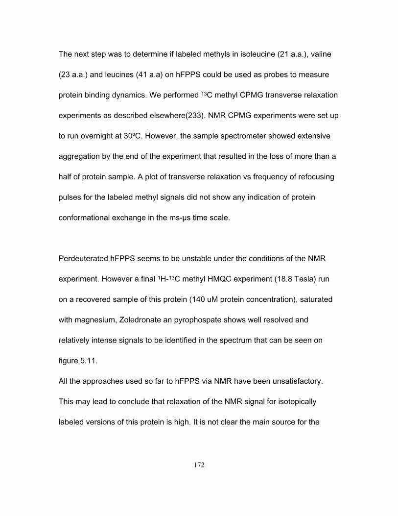
172
The next step was to determine if labeled methyls in isoleucine (21 a.a.), valine
(23 a.a.) and leucines (41 a.a) on hFPPS could be used as probes to measure
protein binding dynamics. We performed 13C methyl CPMG transverse relaxation
experiments as described elsewhere(233). NMR CPMG experiments were set up
to run overnight at 30⁰C. However, the sample spectrometer showed extensive
aggregation by the end of the experiment that resulted in the loss of more than a
half of protein sample. A plot of transverse relaxation vs frequency of refocusing
pulses for the labeled methyl signals did not show any indication of protein
conformational exchange in the ms-µs time scale.
Perdeuterated hFPPS seems to be unstable under the conditions of the NMR
experiment. However a final 1H-13C methyl HMQC experiment (18.8 Tesla) run
on a recovered sample of this protein (140 uM protein concentration), saturated
with magnesium, Zoledronate an pyrophospate shows well resolved and
relatively intense signals to be identified in the spectrum that can be seen on
figure 5.11.
All the approaches used so far to hFPPS via NMR have been unsatisfactory.
This may lead to conclude that relaxation of the NMR signal for isotopically
labeled versions of this protein is high. It is not clear the main source for the
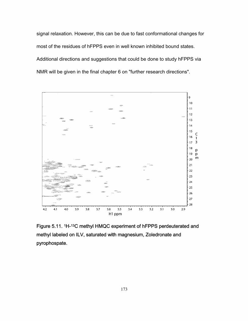
173
signal relaxation. However, this can be due to fast conformational changes for
most of the residues of hFPPS even in well known inhibited bound states.
Additional directions and suggestions that could be done to study hFPPS via
NMR will be given in the final chapter 6 on "further research directions".
Figure 5.11. 1H-13C methyl HMQC experiment of hFPPS perdeuterated and methyl labeled on ILV, saturated with magnesium, Zoledronate and pyrophospate.

174
6. Further research directions
175
6.1. Overview.
The three projects described in this thesis would benefit from further attention.
The first is explained in chapter 3. It involves the electrostatic-driven interaction
between several proline rich peptides and the chicken isoform of the SH3 domain
from the tyrosine kinase Fyn. The second project is described in chapter 4. This
section involved mapping the volume changes that occur as the chicken Fyn SH3
domain binds a proline rich peptide. The final project is explained in chapter 5. It
describes different approaches that were used to study binding between
bisphophonates and human farnesyl pyrophosphate synthase via solution state
protein NMR experiments.
6.2. Electrostatic interactions in the binding pathway of a transient protein
complex studied by NMR and isothermal titration calorimetry.
It is interesting to understand what controls binding kinetics in protein-protein
association. For these reason is important to develop methods to describe
quantitatively binding. Electrostatic driven binding between proteins have been
usually studied using models where binding partners form tight and stable
complexes with lifetimes of hours or days. However many biological processes
rely on transiently-formed complexes with lifetimes in the range of milliseconds.
For these systems, binding processes driven by electrostatics have not been fully
176
studied. We have shown here that this type of binding process may rely less on
electrostatics compared to tight binders. This opens a new area of research in
the study of the association processes of weak, transiently-formed complexes. It
would be interesting explore which non-electrostatic driving forces (hydrophobic
interactions or dipole-dipole interactions) help to accelerate and stabilize the
bound complex in weak, transiently-formed systems and the effect on biological
systems that depend on these interactions.
In this chapter we studied the interaction between the chicken fyn SH3 domain
and a series of proline-rich dodecapeptides. For future studies in this project it
would be interesting to study the effects of mutations within the SH3 domain itself
on the thermodynamics and kinetics of binding to SS, SR and RR peptide. This
would include four protein mutants where residues E98 D99 D100 will be
individually replaced by Q98, N99, N100 and a final fourth protein mutant where
any charged residue outside the binding pocket (D92, E94, E107, E116, D118,
E121 or E129) is replaced by electrostaticaly neutral analog amino acid. This
series of experiments will give a broad picture of how the binding process
between SH3 domains and proline rich peptides is mediated by electrostatics.
More specifically it will show how the specificity binding pocket in the SH3
domain modulates electrostatic binding with proline rich peptides. It would also
enable us to dissect specific electrostatic contributions to binding (formation of
177
ion pairs) from non specific electrostatic interactions (long-range interactions
between charged residues in the peptide and charged residues on the protein
outside the binding pocket).
6.3. Mapping volume changes in the binding pathway of an SH3 domain and a
proline rich peptide
In this chapter we were able to measure for the first time the activation volume of
a protein-ligand binding process. In addition to the novelty of the measurement,
this information can be used to understand changes in the solvent that may drive
the association process. In future work, computational models of hydration
waters could be of particular interest to understand our experimental results.
More specifically, there is an interesting aspect of this project that deserves
further experimental work. According to the results shown in chapter 4, the
change in volume between the transition state and the bound state is around 4
ml mol-1. It will be interesting to confirm if that change in volume is due to the
formation of the hydrogen bond between R–4 in the peptide and D99 in the
protein. A series of binding and kinetic experiments at different pressures
between fyn SH3 domain and SS peptide would easily help to confirm or reject
this hypothesis. According to NMR titrations it is highly probable that SS peptide
and SR peptide bind in the same orientation on the SH3 domain. SR peptide
178
makes a unique hydrogen-bonded ion pair in the binding pocket with the SH3
domain, while the SS peptide, which lacks charged residues, is not able to do so.
Thus the difference in volume between the bound state of the SH3-SS peptide
system and the SH3-SR peptide system should lead to a value close to the
volume for the formation of the hydrogen bond formed between R–4 in the peptide
and D100 in the protein (around 4 mL/mol). This approach is complicated by the
fact that that SS and SR peptides likely have different solvation properties in the
free state.
6.4. NMR experimental approaches to study binding of bisphophonates to human
Farnesyl Pyrophosphate Synthase (hFPPS).
Unfortunately, this project did not provide publishable results. However it would
be valuable to screen different solution conditions to improve the protein stability
of perdeuterated hFPPS. The composition of the NMR buffer would be varied by
adjusting the ionic strength, pH and viscosity. This screening can be done using
techniques such as differential scanning fluorimetry(234). This technique helps to
identify small molecule ligands that stabilize purified proteins. The melting
temperature of the protein is measured following the change in fluorescence of a
dye that has affinity for exposed hydrophobic regions of the protein. Screening of
buffers with different pHs, viscosities (i.e., adding glycerol) or salts may help to
179
improve protein stability. Another option would be to try chemical screening
methods to identify ligands other than bisphophonates that promote hFPPS
stability(235). After finding a suitable range of buffer conditions for the protein,
the binding of a series of different ligands to hFPPS can be characterized. These
include the recently discovered allosteric non-bisphophonate inhibitors of
hFPPS(236). Using differential scanning calorimetry together with intrinsic
binding fluorescence experiments may help to identify ligand that stabilize the
bound complex.
180
References 1. Newton, A. C. (1995) Protein kinase C: structure, function, and regulation. J Biol Chem
270, 28495‐28498 2. Kristiansen, K. (2004) Molecular mechanisms of ligand binding, signaling, and regulation
within the superfamily of G‐protein‐coupled receptors: molecular modeling and mutagenesis approaches to receptor structure and function. Pharmacol Therapeut 103, 21‐80
3. Freiburger, L. A., Baettig, O. M., Sprules, T., Berghuis, A. M., Auclair, K., and Mittermaier, A. K. (2011) Competing allosteric mechanisms modulate substrate binding in a dimeric enzyme. Nature Structural & Molecular Biology 18, 288‐U270
4. Schramm, V. L. (2007) Enzymatic transition state theory and transition state analogue design. J Biol Chem 282, 28297‐28300
5. Qi, S. Y., Groves, J. T., and Chakraborty, A. K. (2001) Synaptic pattern formation during cellular recognition. P Natl Acad Sci USA 98, 6548‐6553
6. Hu, J. M., Toft, D. O., and Seeger, C. (1997) Hepadnavirus assembly and reverse transcription require a multi‐component chaperone complex which is incorporated into nucleocapsids. Embo J 16, 59‐68
7. Miller, D. W., and Dill, K. A. (1997) Ligand binding to proteins: The binding landscape model. Protein Science 6, 2166‐2179
8. Camacho, C. J., Gatchell, D. W., Kimura, S. R., and Vajda, S. (2000) Scoring docked conformations generated by rigid‐body protein‐protein docking. Proteins 40, 525‐537
9. Mobley, D. L., and Dill, K. A. (2009) Binding of small‐molecule ligands to proteins: "what you see" is not always "what you get". Structure 17, 489‐498
10. Macomber, R. S. (1992) An Introduction to Nmr Titration for Studying Rapid Reversible Complexation. Journal of Chemical Education 69, 375‐378
11. Tsai, C. J., Kumar, S., Ma, B. Y., and Nussinov, R. (1999) Folding funnels, binding funnels, and protein function. Protein Science 8, 1181‐1190
12. Mulder, F. A. A., Mittermaier, A., Hon, B., Dahlquist, F. W., and Kay, L. E. (2001) Studying excited states of proteins by NMR spectroscopy. Nat. Struct. Biol. 8, 932‐935
13. McQuarrie, D. A., and Simon, J. D. (1997) Physical chemistry : a molecular approach, University Science Books, Sausalito, Calif.
14. Cantor, C. R., and Schimmel, P. R. (1980) The behavior of biological macromolecules, W. H. Freeman, San Francisco
15. Pilling, M. J., and Seakins, P. W. (1995) Reaction kinetics, Oxford University Press, Oxford ; New York
16. Berg, O. G., and Vonhippel, P. H. (1985) Diffusion‐controlled macromolecular interactions. Annual Review of Biophysics and Biophysical Chemistry 14, 131‐160
17. Smoluchowski, M. (1917) Versuch einer mathematischen theorie der koagulationskinetik kolloider losungen. Z. Phys. Chem. 92, 129‐168
18. Zhou, H. X. (2010) Rate theories for biologists. Q Rev Biophys 43, 219‐293 19. Ubbink, M. (2009) The courtship of proteins: Understanding the encounter complex.
Febs Lett 583, 1060‐1066 20. Janin, J. (1997) The kinetics of protein‐protein recognition. Proteins Struct. Funct. Gen.
28, 153‐161 21. Kahn, D. S. (1949) The Activated Complex of the Protein Molecule. J Phys Colloid Chem
53, 977‐996
181
22. Schramm, V. L. (1998) Enzymatic transition states and transition state analog design. Annu Rev Biochem 67, 693‐720
23. Hoff, J. H. v. t. (1884) Études de dynamique chimique, Muller, Amsterdam, 24. Arrhenius, S. (1889) Über die Reaktionsgeschwindigkeit bei der Inversion von Rohrzucker
durch Säuren, Wilhelm Engelmann 25. Einstein, A., Fürth, R., and Cowper, A. D. (1926) Investigations on the theory of the
Brownian movement, Methuen & Co. ltd., London, 26. Van't Hoff, J. W. (1887) Die Rolle des osmotischen Druckes in der Analogie zwischen
Lösungen und Gasen. Z. physik. Chemie 1, 481‐493 27. Bird, R. B., Stewart, W. E., and Lightfoot, E. N. (2002) Transport phenomena, 2nd, Wiley
international ed., J. Wiley, New York 28. Tellinghuisen, J. (2004) Statistical error in isothermal titration calorimetry. Methods
Enzymol 383, 245‐282 29. Lakowicz, J. R. (2006) Principles of fluorescence spectroscopy, 3rd ed., Springer, New
York 30. Hansen, S. B., Radic, Z., Talley, T. T., Molles, B. E., Deerinck, T., Tsigelny, I., and Taylor, P.
(2002) Tryptophan fluorescence reveals conformational changes in the acetylcholine binding protein. Journal of Biological Chemistry 277, 41299‐41302
31. Musacchio, A., Wilmanns, M., and Saraste, M. (1994) Structure and Function of the Sh3 Domain. Prog Biophys Mol Bio 61, 283‐297
32. Ding, V. D. H., Sheares, B. T., Bergstrom, J. D., Ponpipom, M. M., Perez, L. B., and Poulter, C. D. (1991) Purification and Characterization of Recombinant Human Farnesyl Diphosphate Synthase Expressed in Escherichia‐Coli. Biochem J 275, 61‐65
33. Seet, B. T., Dikic, I., Zhou, M. M., and Pawson, T. (2006) Reading protein modifications with interaction domains. Nat Rev Mol Cell Bio 7, 473‐483
34. Zarrinpar, A., Bhattacharyya, R. P., and Lim, W. A. (2003) The structure and function of proline recognition domains. Sci STKE 2003, RE8
35. Musacchio, A., Noble, M., Pauptit, R., Wierenga, R., and Saraste, M. (1992) Crystal‐Structure of a Src‐Homology‐3 (Sh3) Domain. Nature 359, 851‐855
36. Adzhubei, A. A., Sternberg, M. J. E., and Makarov, A. A. (2013) Polyproline‐II Helix in Proteins: Structure and Function. Journal of Molecular Biology 425, 2100‐2132
37. Li, S. S. C. (2005) Specificity and versatility of SH3 and other proline‐recognition domains: structural basis and implications for cellular signal transduction. Biochem J 390, 641‐653
38. Holt, M. R., and Koffer, A. (2001) Cell motility: proline‐rich proteins promote protrusions. Trends Cell Biol 11, 38‐46
39. Macarthur, M. W., and Thornton, J. M. (1991) Influence of Proline Residues on Protein Conformation. J Mol Biol 218, 397‐412
40. Agrawal, V., and Kishan, K. V. R. (2002) Promiscuous binding nature of SH3 domains to their target proteins. Protein Peptide Lett 9, 185‐193
41. Wilkin, D. J., Kutsunai, S. Y., and Edwards, P. A. (1990) Isolation and Sequence of the Human Farnesyl Pyrophosphate Synthetase Cdna ‐ Coordinate Regulation of the Messenger‐Rnas for Farnesyl Pyrophosphate Synthetase, 3‐Hydroxy‐3‐Methylglutaryl Coenzyme‐a Reductase, and 3‐Hydroxy‐3‐Methylglutaryl Coenzyme‐a Synthase by Phorbol Ester. Journal of Biological Chemistry 265, 4607‐4614
42. Liang, P. H., Ko, T. P., and Wang, A. H. J. (2002) Structure, mechanism and function of prenyltransferases. Eur J Biochem 269, 3339‐3354
182
43. Buhaescu, I., and Izzedine, H. (2007) Mevalonate pathway: A review of clinical and therapeutical implications. Clin Biochem 40, 575‐584
44. Pfeffer, S., and Aivazian, D. (2004) Targeting RAB GTPases to distinct membrane compartments. Nat Rev Mol Cell Bio 5, 886‐896
45. Berzat, A. C., Brady, D. C., Fiordalisi, J. J., and Cox, A. D. (2006) Using inhibitors of prenylation to block localization and transforming activity. Method Enzymol 407, 575‐597
46. Yeganeh, B., Wiechec, E., Ande, S. R., Sharma, P., Moghadam, A. R., Post, M., Freed, D. H., Hashemi, M., Shojaei, S., Zeki, A. A., and Ghavami, S. (2014) Targeting the mevalonate cascade as a new therapeutic approach in heart disease, cancer and pulmonary disease. Pharmacol Therapeut 143, 87‐110
47. Luckman, S. P., Hughes, D. E., Coxon, F. P., Russell, R. G. G., and Rogers, M. J. (1998) Nitrogen‐containing bisphosphonates inhibit the mevalonate pathway and prevent post‐translational prenylation of GTP‐binding proteins, including Ras. J Bone Miner Res 13, 581‐589
48. Drake, M. T., Clarke, B. L., and Khosla, S. (2008) Bisphosphonates: Mechanism of action and role in clinical practice. Mayo Clin Proc 83, 1032‐1045
49. Coleman, R. (2011) The use of bisphosphonates in cancer treatment. Ann Ny Acad Sci 1218, 3‐14
50. Kavanagh, K. L., Guo, K. D., Dunford, J. E., Wu, X. Q., Knapp, S., Ebetino, F. H., Rogers, M. J., Russell, R. G. G., and Oppermann, U. (2006) The molecular mechanism of nitrogen‐containing bisphosphonates as anti osteoporosis drugs. Proceedings of the National Academy of Sciences of the United States of America 103, 7829‐7834
51. Hosfield, D. J., Zhang, Y. M., Dougan, D. R., Broun, A., Tari, L. W., Swanson, R. V., and Finn, J. (2004) Structural basis for bisphosphonate‐mediated inhibition of isoprenoid biosynthesis. Journal of Biological Chemistry 279, 8526‐8529
52. Cavanagh, J. (1996) Protein NMR spectroscopy: Principles and practice, Academic Press, San Diego
53. Mittermaier, A., and Kay, L. E. (2006) New tools provide new insights in NMR studies of protein dynamics. Science 312, 224‐228
54. Ikura, M., Clore, G. M., Gronenborn, A. M., Zhu, G., Klee, C. B., and Bax, A. (1992) Solution structure of a calmodulin‐target peptide complex by multidimensional NMR. Science 256, 632‐638
55. Walters, K. J., Ferentz, A. E., Hare, B. J., Hidalgo, P., Jasanoff, A., Matsuo, H., and Wagner, G. (2001) Characterizing protein‐protein complexes and oligomers by nuclear magnetic resonance spectroscopy. Nuclear Magnetic Resonance of Biological Macromolecules, Pt B 339, 238‐258
56. Jung, Y. S., Cai, M. L., and Clore, G. M. (2010) Solution Structure of the IIA(Chitobiose)‐IIBChitobiose Complex of the N,N '‐Diacetylchitobiose Branch of the Escherichia coli Phosphotransferase System. Journal of Biological Chemistry 285, 4173‐4184
57. Finerty, P. J., Mittermaier, A. K., Muhandiram, R., Kay, L. E., and Forman‐Kay, J. D. (2005) NMR dynamics‐derived insights into the binding properties of a peptide interacting with an SH2 domain. Biochemistry 44, 694‐703
58. Boehr, D. D., McElheny, D., Dyson, H. J., and Wright, P. E. (2006) The dynamic energy landscape of dihydrofolate reductase catalysis. Science 313, 1638‐1642
59. Sugase, K., Dyson, H. J., and Wright, P. E. (2007) Mechanism of coupled folding and binding of an intrinsically disordered protein. Nature 447, 1021‐U1011
183
60. Iwahara, J., and Clore, G. M. (2006) Detecting transient intermediates in macromolecular binding by paramagnetic NMR. Nature 440, 1227‐1230
61. Meyer, B., and Peters, T. (2003) NMR spectroscopy techniques for screening and identifying ligand binding to protein receptors. Angew Chem Int Ed Engl 42, 864‐890
62. Shuker, S. B., Hajduk, P. J., Meadows, R. P., and Fesik, S. W. (1996) Discovering high‐affinity ligands for proteins: SAR by NMR. Science 274, 1531‐1534
63. Zarrine‐Afsar, A., Mittermaier, A., Kay, L. E., and Davidson, A. R. (2006) Protein stabilization by specific binding of guanidinium to a functional arginine‐binding surface on an SH3 domain. Protein Science 15, 162‐170
64. Chen, Y., Reizer, J., Saier, M. H., Fairbrother, W. J., and Wright, P. E. (1993) Mapping of the binding interfaces of the proteins of the bacterial phosphotransferase system, HPr and IIAglc. Biochemistry 32, 32‐37
65. Liu, Z. H., Sun, C. H., Olejniczak, E. T., Meadows, R. P., Betz, S. F., Oost, T., Herrmann, J., Wu, J. C., and Fesik, S. W. (2000) Structural basis for binding of Smac/DIABLO to the XIAP BIR3 domain. Nature 408, 1004‐1008
66. Demers, J. P., and Mittermaier, A. (2009) Binding Mechanism of an SH3 Domain Studied by NMR and ITC. Journal of the American Chemical Society 131, 4355‐4367
67. Schuck, P. (1996) Kinetics of ligand binding to receptor immobilized in a polymer matrix, as detected with an evanescent wave biosensor .1. A computer simulation of the influence of mass transport. Biophysical J. 70, 1230‐1249
68. Tochtrop, G. P., Richter, K., Tang, C., Toner, J. J., Covey, D. F., and Cistola, D. P. (2002) Energetics by NMR: site‐specific binding in a positively cooperative system. Proc. Natl. Acad. Sci. U.S.A. 99, 1847‐1852
69. Tugarinov, V., Choy, W. Y., Orekhov, V. Y., and Kay, L. E. (2005) Solution NMR‐derived global fold of a monomeric 82‐kDa enzyme. Proceedings of the National Academy of Sciences of the United States of America 102, 622‐627
70. Bodenhausen, G., and Ruben, D. J. (1980) Natural abundance nitrogen‐15 NMR by enhanced heteronuclear spectroscopy. Chemical Physics Letters 69, 185‐189
71. Loria, J. P., Rance, M., and Palmer, A. G. (1999) A relaxation‐compensated Carr‐Purcell‐Meiboom‐Gill sequence for characterizing chemical exchange by NMR spectroscopy. Journal of the American Chemical Society 121, 2331‐2332
72. Farrow, N. A., Zhang, O., Forman‐Kay, J. D., and Kay, L. E. (1994) A heteronuclear correlation experiment for simultaneous determination of 15N longitudinal decay and chemical exchange rates of systems in slow equilibrium. J. Biomol. NMR 4, 727‐734
73. Renzoni, D. A., Pugh, D. J. R., Siligardi, G., Das, P., Morton, C. J., Rossi, C., Waterfield, M. D., Campbell, I. D., and Ladbury, J. E. (1996) Structural and thermodynamic characterization of the interaction of the SH3 domain from Fyn with the proline‐rich binding site on the p85 subunit of PI3‐kinase. Biochemistry 35, 15646‐15653
74. Gardner, K. H., and Kay, L. E. (1998) The use of 2H, 13C, 15N multidimensional NMR to study the structure and dynamics of proteins. Annu. Rev. Biophys. Biomol. Struct. 27, 357‐406
75. Marley, J., Lu, M., and Bracken, C. (2001) A method for efficient isotopic labeling of recombinant proteins. J Biomol NMR 20, 71‐75
76. Bai, Y. W., Milne, J. S., Mayne, L., and Englander, S. W. (1993) Primary structure effects on peptide group hydrogen exchange. Proteins‐Structure Function and Genetics 17, 75‐86
184
77. Sugase, K., Lansing, J. C., Dyson, H. J., and Wright, P. E. (2007) Tailoring relaxation dispersion experiments for fast‐associating protein complexes. Journal of the American Chemical Society 129, 13406‐+
78. Johnson, B. A., and Blevins, R. A. (1994) NMR View ‐ A computer program for the visualization and analysis of NMR data. Journal of Biomolecular Nmr 4, 603‐614
79. van Beek, J. D. (2007) matNMR: A flexible toolbox for processing, analyzing and visualizing magnetic resonance data in Matlab((R)). Journal of Magnetic Resonance 187, 19‐26
80. Vranken, W. F., Boucher, W., Stevens, T. J., Fogh, R. H., Pajon, A., Llinas, P., Ulrich, E. L., Markley, J. L., Ionides, J., and Laue, E. D. (2005) The CCPN data model for NMR spectroscopy: Development of a software pipeline. Proteins‐Structure Function and Bioinformatics 59, 687‐696
81. Gunther, U. L., Ludwig, C., and Ruterjans, H. (2000) NMRLAB ‐ Advanced NMR data processing in MATLAB. Journal of Magnetic Resonance 145, 201‐208
82. Delaglio, F., Grzesiek, S., Vuister, G. W., Zhu, G., Pfeifer, J., and Bax, A. (1995) NMRPipe: a multidimensional spectral processing system based on UNIX pipes. J. Biomol. NMR 6, 277‐293
83. Gunther, U. L., and Schaffhausen, B. (2002) NMRKIN: Simulating line shapes from two‐dimensional spectra of proteins upon ligand binding. Journal of Biomolecular Nmr 22, 201‐209
84. Vetterling, W. T., Press, W. H., Teukolsky, S. A., and Flannery, B. R. (1988) Numerical Recipes in C, Cambridge University Press, Cambridge
85. Langmuir, I. (1916) The constitution and fundamental properties of solids and liquids Part I Solids. Journal of the American Chemical Society 38, 2221‐2295
86. Wiseman, T., Williston, S., Brandts, J. F., and Lin, L. N. (1989) Rapid measurement of binding constants and heats of binding using a new titration calorimeter. Analytical Biochemistry 179, 131‐137
87. Gutowsky, H. S., and Saika, A. (1953) Dissociation, chemical exchange, and the proton magnetic resonance in some aqueous electrolytes. Journal of Chemical Physics 21, 1688‐1694
88. McConnell, H. M. (1958) Reaction rates by Nuclear Magnetic Resonance. Journal of Chemical Physics 28, 430‐431
89. Rogers, M. T., and Woodbrey, J. C. (1962) Proton magnetic resonance study of hindered internal rotation in some substituted N,N‐dimethylamides. Journal of Physical Chemistry 66, 540‐&
90. Gupta, R. K., Pitner, T. P., and Wasylishen, R. (1974) Fourier transform NMR of exchanging chemical systems. Journal of Magnetic Resonance 13, 383‐385
91. Mittag, T., Schaffhausen, B., and Gunther, U. L. (2004) Tracing kinetic intermediates during ligand binding. Journal of the American Chemical Society 126, 9017‐9023
92. Carr, H. Y., and Purcell, E. M. (1954) Effects of diffusion on free precession in nuclear magnetic resonance experiments. Physical Review 94, 630‐638
93. Meiboom, S., and Gill, D. (1958) Modified spin echo method for measureing nuclear relaxation times. Review of Scientific Instruments 29, 688‐691
94. Palmer, A. G., Kroenke, C. D., and Loria, J. P. (2001) Nuclear magnetic resonance methods for quantifying microsecond‐to‐millisecond motions in biological macromolecules. Nuclear Magnetic Resonance of Biological Macromolecules, Pt B 339, 204‐238
185
95. Korzhnev, D. M., and Kay, L. E. (2008) Probing invisible, low‐populated states of protein molecules by relaxation dispersion NMR spectroscopy: An application to protein folding. Accounts of Chemical Research 41, 442‐451
96. Hahn, E. L. (1950) Spin Echoes. Physical Review 80, 580 97. Esadze, A., Li, D. W., Wang, T. Z., Bruschweiler, R., and Iwahara, J. (2011) Dynamics of
Lysine Side‐Chain Amino Groups in a Protein Studied by Heteronuclear H‐1‐N‐15 NMR Spectroscopy. Journal of the American Chemical Society 133, 909‐919
98. Ishima, R., Baber, J., Louis, J. M., and Torchia, D. A. (2004) Carbonyl carbon transverse relaxation dispersion measurements and ms‐mu s timescale motion in a protein hydrogen bond network. Journal of Biomolecular Nmr 29, 187‐198
99. Ishima, R., and Torchia, D. A. (2003) Extending the range of amide proton relaxation dispersion experiments in proteins using a constant‐time relaxation‐compensated CPMG approach. Journal of Biomolecular Nmr 25, 243‐248
100. Korzhnev, D. M., Neudecker, P., Mittermaier, A., Orekhov, V. Y., and Kay, L. E. (2005) Multiple‐site exchange in proteins studied with a suite of six NMR relaxation dispersion experiments: An application to the folding of a Fyn SH3 domain mutant. Journal of the American Chemical Society 127, 15602‐15611
101. Mulder, F. A. A., Skrynnikov, N. R., Hon, B., Dahlquist, F. W., and Kay, L. E. (2001) Measurement of slow (mu s‐ms) time scale dynamics in protein side chains by N‐15 relaxation dispersion NMR spectroscopy: Application to Asn and Gln residues in a cavity mutant of T4 lysozyme. Journal of the American Chemical Society 123, 967‐975
102. Skrynnikov, N. R., Mulder, F. A. A., Hon, B., Dahlquist, F. W., and Kay, L. E. (2001) Probing slow time scale dynamics at methyl‐containing side chains in proteins by relaxation dispersion NMR measurements: Application to methionine residues in a cavity mutant of T4 lysozyme. Journal of the American Chemical Society 123, 4556‐4566
103. Lundstrom, P., Lin, H., and Kay, L. E. (2009) Measuring C‐13(beta) chemical shifts of invisible excited states in proteins by relaxation dispersion NMR spectroscopy. Journal of Biomolecular Nmr 44, 139‐155
104. Baldwin, A. J., Hansen, D. F., Vallurupalli, P., and Kay, L. E. (2009) Measurement of Methyl Axis Orientations in Invisible, Excited States of Proteins by Relaxation Dispersion NMR Spectroscopy. Journal of the American Chemical Society 131, 11939‐11948
105. Hansen, D. F., Vallurupalli, P., and Kay, L. E. (2009) Measurement of Methyl Group Motional Parameters of Invisible, Excited Protein States by NMR Spectroscopy. Journal of the American Chemical Society 131, 12745‐12754
106. Vallurupalli, P., Hansen, D. F., Stollar, E., Meirovitch, E., and Kay, L. E. (2007) Measurement of bond vector orientations in invisible excited states of proteins. Proceedings of the National Academy of Sciences of the United States of America 104, 18473‐18477
107. Palmer, A. G., and Massi, F. (2006) Characterization of the dynamics of biomacromolecules using rotating‐frame spin relaxation NMR spectroscopy. Chemical Reviews 106, 1700‐1719
108. Hansen, D. F., Vallurupalli, P., and Kay, L. E. (2008) An improved N‐15 relaxation dispersion experiment for the measurement of millisecond time‐scale dynamics in proteins. Journal of Physical Chemistry B 112, 5898‐5904
109. Ishima, R., and Torchia, D. A. (2006) Accuracy of optimized chemical‐exchange parameters derived by fitting CPMG R2 dispersion profiles when R2(0a) = R2(0b). Journal of Biomolecular NMR 34, 209‐219
186
110. Korzhnev, D. M., Salvatella, X., Vendruscolo, M., Di Nardo, A. A., Davidson, A. R., Dobson, C. M., and Kay, L. E. (2004) Low‐populated folding intermediates of Fyn SH3 characterized by relaxation dispersion NMR. Nature 430, 586‐590
111. Carver, J. P., and Richards, R. E. (1972) General 2‐site solution for chemical exchange produced dependence of T2 upon Carr‐Purcell pulse separation. Journal of Magnetic Resonance 6, 89‐&
112. Davis, D. G., Perlman, M. E., and London, R. E. (1994) Direct measurements of the dissociation rate constant for inhibitor enzyme complexes via the T1rho and T2(CPMG) methods. Journal of Magnetic Resonance Series B 104, 266‐275
113. Luz, Z., and Meiboom, S. (1963) Nuclear Magnetic Resonance Study of Protolysis of Trimethylammonium Ion in Aqueous Solution ‐ Order of Reaction with Respect to Solvent. Journal of Chemical Physics 39, 366‐&
114. Kovrigin, E. L., Kempf, J. G., Grey, M. J., and Loria, J. P. (2006) Faithful estimation of dynamics parameters from CPMG relaxation dispersion measurements. Journal of Magnetic Resonance 180, 93‐104
115. Millet, O., Loria, J. P., Kroenke, C. D., Pons, M., and Palmer, A. G. (2000) The static magnetic field dependence of chemical exchange linebroadening defines the NMR chemical shift time scale. J. Am. Chem. Soc. 122, 2867‐2877
116. Mulder, F. A. A., Mittermaier, A., Hon, B., Dahlquist, F. W., and Kay, L. E. (2001) Studying excited states of proteins by NMR spectroscopy. Nature Structural Biology 8, 932‐935
117. Amman, C., Meier, P., and Merbach, A. E. (1982) A simple multinuclear NMR thermometer. Journal of Magnetic Resonance 46, 319‐321
118. Findeisen, M., Brand, T., and Berger, S. (2007) A 1H‐NMR thermometer suitable for cryoprobes. Magnetic resonance in chemistry : MRC 45, 175‐178
119. Hindman, J. C. (1966) Proton resonance shift of water in gas and liquid states. Journal of Chemical Physics 44, 4582‐&
120. Radic, Z., Kirchhoff, P. D., Quinn, D. M., McCammon, J. A., and Taylor, P. (1997) Electrostatic influence on the kinetics of ligand binding to acetylcholinesterase. Distinctions between active center ligands and fasciculin. J. Biol. Chem. 272, 23265‐23277
121. Foote, J., and Milstein, C. (1991) Kinetic maturation of an immune response. Nature 352, 530‐532
122. Wang, Y. H., Shen, B. J., and Sebald, W. (1997) A mixed‐charge pair in human interleukin 4 dominates high‐affinity interaction with the receptor alpha chain. Proc. Natl. Acad. Sci. USA 94, 1657‐1662
123. Jucovic, M., and Hartley, R. W. (1996) Protein‐protein interaction: A genetic selection for compensating mutations at the barnase‐barstar interface. Proc. Natl. Acad. Sci. USA 93, 2343‐2347
124. Schreiber, G., and Fersht, A. R. (1996) Rapid, electrostatically assisted association of proteins. Nat. Struct. Biol. 3, 427‐431
125. Zhou, H. X. (1997) Enhancement of protein‐protein association rate by interaction potential: accuracy of prediction based on local Boltzmann factor. Biophys. J. 73, 2441‐2445
126. Northrup, S. H., and Erickson, H. P. (1992) Kinetics of protein‐protein association explained by Brownian dynamics computer simulation. Proc. Natl. Acad. Sci. USA 89, 3338‐3342
187
127. Gabdoulline, R. R., and Wade, R. C. (2002) Biomolecular diffusional association. Curr. Op. Struct. Biol. 12, 204‐213
128. Wallis, R., Moore, G. R., James, R., and Kleanthous, C. (1995) Protein‐Protein Interactions in Colicin E9 Dnase‐Immunity Protein Complexes .1. Diffusion‐Controlled Association and Femtomolar Binding for the Cognate Complex. Biochemistry 34, 13743‐13750
129. Shen, B. J., Hage, T., and Sebald, W. (1996) Global and local determinants for the kinetics of interleukin‐4/interleukin‐4 receptor alpha chain interaction ‐ A biosensor study employing recombinant interleukin‐4‐binding protein. Eur. J. Biochem. 240, 252‐261
130. Zhou, H. X. (2001) Disparate Ionic‐Strength Dependencies of On and Off Rates in Protein–Protein Association. Biopolymers 59, 427‐433
131. Alsallaq, R., and Zhou, H. X. (2008) Electrostatic rate enhancement and transient complex of protein‐protein association. Proteins Struct. Funct. Bioinf. 71, 320‐335
132. Alsallaq, R., and Zhou, H.‐X. (2007) Prediction of protein‐protein association rates from a transition‐state theory. Structure 15, 215‐224
133. Pilling, M., and Seakins, P. (1995) Reaction Kinetics, Oxford University Press, Oxford 134. Szabo, A., Shoup, D., Northrup, S., and McCammon, J. A. (1982) Stochastically gated
diffusion‐influenced reactions. J. Chem. Phys. 77, 4484‐4493 135. Sommer, J., Jonah, C., Fukuda, R., and Bersohn, R. (1982) Production and subsequent
2nd‐order decomposition of protein disulfide anions ‐ lengthy collisions between proteins. J. Mol. Biol. 159, 721‐744
136. Camacho, C., Kimura, S., DeLisi, C., and Vajda, S. (2000) Kinetics of desolvation‐mediated protein‐protein binding. Biophysical J. 78, 1094‐1105
137. Camacho, C., Weng, Z., Vajda, S., and DeLisi, C. (1999) Free energy landscapes of encounter complexes in protein‐protein association. Biophysical J. 76, 1166‐1178
138. Northrup, S. H., Thomasson, K. A., Miller, C. M., Barker, P. D., Eltis, L. D., Guillemette, J. G., Inglis, S. C., and Mauk, A. G. (1993) Effects of charged amino acid mutations on the bimolecular kinetics of reduction of yeast iso‐1‐ferricytochrome c by bovine ferrocytochrome b5. Biochemistry 32, 6613‐6623
139. Vijayakumar, M., Wong, K. Y., Schreiber, G., Fersht, A. R., Szabo, A., and Zhou, H. X. (1998) Electrostatic enhancement of diffusion‐controlled protein‐protein association: Comparison of theory and experiment on barnase and barstar. J. Mol. Biol. 278, 1015‐1024
140. Schreiber, G., and Fersht, A. R. (1993) Interaction of barnase with its polypeptide inhibitor barstar studied by protein engineering. Biochemistry 32, 5145‐5150
141. Escobar, L., Root, M. J., and MacKinnon, R. (1993) Influence of protein surface charge on the bimolecular kinetics of a potassium channel peptide inhibitor. Biochemistry 32, 6982‐6987
142. Wallis, R., Leung, K. Y., Pommer, A. J., Videler, H., Moore, G. R., James, R., and Kleanthous, C. (1995) Protein‐protein interactions in colicin E9 DNase‐immunity protein complexes. 2. Cognate and noncognate interactions that span the millimolar to femtomolar affinity range. Biochemistry 34, 13751‐13759
143. Wendt, H., Leder, L., Harma, H., Jelesarov, I., Baici, A., and Bosshard, H. R. (1997) Very rapid, ionic strength‐dependent association and folding of a heterodimeric leucine zipper. Biochemistry 36, 204‐213
144. Volkov, A. N., Ubbink, M., and van Nuland, N. A. J. (2010) Mapping the encounter state of a transient protein complex by PRE NMR spectroscopy. J. Biomol. NMR 48, 225‐236
188
145. Tang, C., Iwahara, J., and Clore, G. M. (2006) Visualization of transient encounter complexes in protein‐protein association. Nature 444, 383‐386
146. Sydor, J. R., Engelhard, M., Wittinghofer, A., Goody, R. S., and Herrmann, C. (1998) Transient kinetic studies on the interaction of ras and the Ras‐binding domain of c‐Raf‐1 reveal rapid equilibration of the complex. Biochemistry 37, 14292‐14299
147. Stone, S. R., Dennis, S., and Hofsteenge, J. (1989) Quantitative evaluation of the contribution of ionic interactions to the formation of the thrombin‐hirudin complex. Biochemistry 28, 6857‐6863
148. Taylor, M. G., Rajpal, A., and Kirsch, J. F. (1998) Kinetic epitope mapping of the chicken lysozyme.HyHEL‐10 Fab complex: delineation of docking trajectories. Protein Sci. 7, 1857‐1867
149. Altschuh, D., Dubs, M. C., Weiss, E., Zeder‐Lutz, G., and Van Regenmortel, M. H. (1992) Determination of kinetic constants for the interaction between a monoclonal antibody and peptides using surface plasmon resonance. Biochemistry 31, 6298‐6304
150. England, P., Bregegere, F., and Bedouelle, H. (1997) Energetic and kinetic contributions of contact residues of antibody D1.3 in the interaction with lysozyme. Biochemistry 36, 164‐172
151. Vallurupalli, P., Hansen, D. F., Stollar, E., Meirovitch, e., and Kay, L. E. (2007) Measurement of bond vector orientations in invisible excited states of proteins. Proc. Natl. Acad. Sci. USA 104, 18473–18477
152. Demers, J. P., and Mittermaier, A. (2009) Binding Mechanism of an SH3 Domain Studied by NMR and ITC. J. Am. Chem. Soc. 131, 4355‐4367
153. Mittermaier, A. K., and Kay, L. E. (2009) Observing biological dynamics at atomic resolution using NMR. Trends Biochem. Sci. 34, 601‐611
154. Palmer, A. G., Kroenke, C. D., and Loria, J. P. (2001) NMR methods for quantifying microsecond‐to‐millisecond motions in biological macromolecules. Methods Enzymol. 339, 204‐238
155. Hansen, A. F., Vallurupalli, P., and Kay, L. E. (2008) An improved 15N relaxation dispersion experiment for the measurement of millisecond time‐scale dynamics in proteins. J. Phys. Chem. B 112, 5898‐5904
156. Yu, H., Chen, J. K., Feng, S., Dalgarno, D. C., Brauer, A. W., and Schreiber, S. L. (1994) Structural basis for the binding of proline‐rich peptides to SH3 domains. Cell 76, 933‐945
157. Mayer, B. J. (2001) SH3 domains: complexity in moderation. J. Cell Sci. 114, 1253‐1263 158. Hansen, D. F., Vallurupalli, P., Lundstrom, P., Neudecker, P., and Kay, L. E. (2008) Probing
Chemical Shifts of Invisible States of Proteins with Relaxation Dispersion NMR Spectroscopy: How Well Can We Do? J. Am. Chem. Soc. 130, 2667‐2675
159. Feng, S. B., Kasahara, C., Rickles, R. J., and Schreiber, S. L. (1995) Specific interactions outside the proline‐rich core of two classes of Src homology 3 ligands. Proc. Natl. Acad. Sci. U. S. A. 92, 12408‐12415
160. Mittermaier, A., and Kay, L. E. (2004) The response of internal dynamics to hydrophobic core mutations in the SH3 domain from the Fyn tyrosine kinase. Protein Sci. 13, 1088‐1099
161. Bolzani, R., Ruggeri, F., and Olivo, O. M. (1979) Average normal temperature of the chicken in the morning and after 1‐2 days of fasting. Bollettino della Societa italiana di biologia sperimentale 55, 1618‐1622
189
162. Wishart, D. S., Bigam, C. G., Yao, J., Abildgaard, F., Dyson, H. J., Oldfield, E., Markley, J. L., and Sykes, B. D. (1995) 1H, 13C and 15N chemical shift referencing in biomolecular NMR. J. Biomol. NMR 6, 135‐140
163. Luz, Z., and Meiboom, S. (1963) Nuclear Magnetic Resonance Study of the Protolysis of Trimethylammonium Ion in Aqueous Solution—Order of the Reaction with Respect to Solvent. J. Chem. Phys. 39, 366
164. Carver, J. P., and Richards, R. E. (1972) A general two‐site solution for the chemical exchange produced dependence of T2 upon the Carr‐Purcell pulse separation. J. Magn. Reson. 6, 89‐105
165. Ishima, R., and Torchia, D. (2005) Error estimation and global fitting in transverse‐relaxation dispersion experiments to determine chemical‐exchange parameters. J. Biomol. NMR 32, 41‐54
166. Efron, B., and Tibshirani, R. (1986) Bootstrap methods for standard errors, confidence intervals and other measures of statistical accuracy. Stat. Sci. 1, 54‐77
167. Di Nardo, A. A., Larson, S. M., and Davidson, A. R. (2003) The relationship between conservation, thermodynamic stability, and function in the SH3 domain hydrophobic core. Journal of Molecular Biology 333, 641‐655
168. Cantor, C., and Schimmel, P. (1980) Biophysical Chemistry Part III: The behaviour of biological macromolecules, W.H. Freeman and Co.
169. Pace, C. N., Vajdos, F., Fee, L., Grimsley, G., and Gray, T. (1995) How to Measure and Predict the Molar Absorption Coefficient of a Protein. Prot. Sci.
4, 2411‐2423 170. Smith, A. J. (1997) Amino Acid Analysis. Meth. Enz. 289, 419‐426 171. Melander, W., and Horvath, C. (1977) Salt effects on hydrophobic interactions in
precipitation and chromatography of proteins ‐ interpretation of lyotropic series. Arch. Biochem. Biophys. 183, 200‐215
172. Bennaim, A., and Yaacobi, M. (1974) Effects of solutes on strength of hydrophobic interaction and its temperature‐dependence. Journal of Physical Chemistry 78, 170‐175
173. Docherty, H., Galindo, A., Sanz, E., and Vega, C. (2007) Investigation of the salting out of methane from aqueous electrolyte solutions using computer simulations. J. Phys. Chem. B 111, 8993‐9000
174. Segur, J. B., and Oberstar, H. E. (1951) Viscosity of glycerol and its aqueous solutions. Industrial and Engineering Chemistry 43, 2117‐2120
175. Schreiber, G. (2002) Kinetic studies of protein‐protein interactions. Curr. Opin. Struct. Biol. 12, 41‐47
176. Eyring, H. (1935) The Activated Complex in Chemical Reactions. J. Chem. Phys. 3, 107‐115
177. Wherland, S., and Gray, H. B. (1976) Metalloprotein electron‐transfer reactions ‐ analysis of reactivity of horse heart cytochrome‐C with inorganic complexes. Proc. Natl. Acad. Sci. U. S. A. 73, 2950‐2954
178. Alberty, R. A., and Hammes, G. G. (1958) Application of the theory of diffusion‐controlled reactions to enzyme kinetics. Journal of Physical Chemistry 62, 154‐159
179. Buckle, A. M., Schreiber, G., and Fersht, A. R. (1994) Protein‐protein recognition ‐ crystal structural‐analysis of a barnase barstar complex at 2.0‐angstrom resolution. Biochemistry 33, 8878‐8889
190
180. Xu, D., Lin, S. L., and Nussinov, R. (1997) Protein binding versus protein folding: The role of hydrophilic bridges in protein associations. J. Mol. Biol. 265, 68‐84
181. Fitos, I., Heremans, K., and Loontiens, F. G. (1979) Binding Study of 4‐Methylumbelliferyl Alpha‐D‐Mannopyranoside to Dimeric Concanavalin‐a under High‐Pressure. React Kinet Catal L 12, 393‐397
182. Li, T. M., Hook, J. W., Drickamer, H. G., and Weber, G. (1976) Effects of Pressure Upon Fluorescence of Riboflavin Binding‐Protein and Its Flavin Mononucleotide Complex. Biochemistry 15, 3205‐3211
183. Heremans, K., Snauwaert, J., and Rijkenberg, J. (1980) Stopped‐Flow Apparatus for the Study of Fast Reactions in Solution under High‐Pressure. Rev Sci Instrum 51, 806‐808
184. Torgerson, P. M., Drickamer, H. G., and Weber, G. (1979) Inclusion Complexes of Poly‐Beta‐Cyclodextrin ‐ Model for Pressure Effects Upon Ligand‐Protein Complexes. Biochemistry 18, 3079‐3083
185. Torgerson, P. M., Drickamer, H. G., and Weber, G. (1980) Effect of Hydrostatic‐Pressure Upon Ethidium‐Bromide Association with Transfer Ribonucleic‐Acid. Biochemistry 19, 3957‐3960
186. Visser, A. J. W. G., Li, T. M., Drickamer, H. G., and Weber, G. (1977) Volume Changes in Formation of Internal Complexes of Flavinyltryptophan Peptides. Biochemistry 16, 4883‐4886
187. Dubins, D. N., Filfil, R., Macgregor, R. B., and Chalikian, T. V. (2000) Role of water in protein‐ligand interactions: Volumetric characterization of the binding of 2 '‐CMP and 3 '‐CMP to ribonuclease A. J Phys Chem B 104, 390‐401
188. Brandts, J. F., Oliveira, R. J., and Westort, C. (1970) Thermodynamics of Protein Denaturation ‐ Effect of Pressure on Denaturation of Ribonuclease‐A. Biochemistry 9, 1038‐&
189. Gill, S. J., and Glogovsk.Rl. (1965) Influence of Pressure on Reversible Unfolding of Ribonuclease and Poly‐Gamma‐Benzyl‐L‐Glutamate. Journal of Physical Chemistry 69, 1515‐&
190. Hawley, S. A. (1971) Reversible Pressure‐Temperature Denaturation of Chymotrypsinogen. Biochemistry 10, 2436‐&
191. Frye, K. J., and Royer, C. A. (1998) Probing the contribution of internal cavities to the volume change of protein unfolding under pressure. Protein Science 7, 2217‐2222
192. Rouget, J. B., Aksel, T., Roche, J., Saldana, J. L., Garcia, A. E., Barrick, D., and Royer, C. A. (2011) Size and Sequence and the Volume Change of Protein Folding. J Am Chem Soc 133, 6020‐6027
193. Schweiker, K. L., Fitz, V. W., and Makhatadze, G. I. (2009) Universal Convergence of the Specific Volume Changes of Globular Proteins upon Unfolding. Biochemistry 48, 10846‐10851
194. Roche, J., Caro, J. A., Norberto, D. R., Barthe, P., Roumestand, C., Schlessman, J. L., Garcia, A. E., Garcia‐Moreno, B., and Royer, C. A. (2012) Cavities determine the pressure unfolding of proteins. Proceedings of the National Academy of Sciences of the United States of America 109, 6945‐6950
195. Low, P. S., and Somero, G. N. (1975) Protein Hydration Changes during Catalysis ‐ New Mechanism of Enzymic Rate‐Enchancement and Ion Activation Inhibition of Catalysis. P Natl Acad Sci USA 72, 3305‐3309
196. Schramm, V. L. (1998) Enzymatic transition states and transition state analog design. Annu Rev Biochem 67, 693‐720
191
197. Schreiber, G., and Fersht, A. R. (1993) Interaction of barnase with its polypeptide inhibitor barstar studied by protein engineering. Biochemistry 32, 5145‐5150
198. Altschuh, D., Dubs, M. C., Weiss, E., Zederlutz, G., and Vanregenmortel, M. H. V. (1992) Determination of Kinetic Constants for the Interaction between a Monoclonal‐Antibody and Peptides Using Surface‐Plasmon Resonance. Biochemistry 31, 6298‐6304
199. Mittermaier, A., and Kay, L. E. (2006) Review ‐ New tools provide new insights in NMR studies of protein dynamics. Science 312, 224‐228
200. Palmer, A. G., 3rd, Kroenke, C. D., and Loria, J. P. (2001) Nuclear magnetic resonance methods for quantifying microsecond‐to‐millisecond motions in biological macromolecules. Methods Enzymol 339, 204‐238
201. Chalikian, T. V., and Filfil, R. (2003) How large are the volume changes accompanying protein transitions and binding? Biophys Chem 104, 489‐499
202. Yu, H. T., Chen, J. K., Feng, S. B., Dalgarno, D. C., Brauer, A. W., and Schreiber, S. L. (1994) Structural Basis for the Binding of Proline‐Rich Peptides to Sh3 Domains. Cell 76, 933‐945
203. Low, P. S., and Somero, G. N. (1975) Activation Volumes in Enzymic Catalysis ‐ Their Sources and Modification by Low‐Molecular‐Weight Solutes. Proceedings of the National Academy of Sciences of the United States of America 72, 3014‐3018
204. Mittermaier, A., and Kay, L. E. (2004) The response of internal dynamics to hydrophobic core mutations in the SH3 domain from the Fyn tyrosine kinase. Protein Science 13, 1088‐1099
205. Dellarole, M., and Royer, C. A. (2014) High‐pressure fluorescence applications. Methods Mol Biol 1076, 53‐74
206. Lee, B., and Richards, F. M. (1971) Interpretation of Protein Structures ‐ Estimation of Static Accessibility. Journal of Molecular Biology 55, 379‐&
207. Richards, F. M. (1977) Areas, Volumes, Packing, and Protein‐Structure. Annual Review of Biophysics and Bioengineering 6, 151‐176
208. Connolly, M. L. (1983) Analytical Molecular‐Surface Calculation. Journal of Applied Crystallography 16, 548‐558
209. Voss, N. R., and Gerstein, M. (2010) 3V: cavity, channel and cleft volume calculator and extractor. Nucleic Acids Research 38, W555‐W562
210. Ogura, K., and Okamura, H. (2013) Conformational change of Sos‐derived proline‐rich peptide upon binding Grb2 N‐terminal SH3 domain probed by NMR. Scientific Reports 3
211. Musacchio, A., Saraste, M., and Wilmanns, M. (1994) High‐Resolution Crystal‐Structures of Tyrosine Kinase Sh3 Domains Complexed with Proline‐Rich Peptides. Nature Structural Biology 1, 546‐551
212. Dundas, J., Ouyang, Z., Tseng, J., Binkowski, A., Turpaz, Y., and Liang, J. (2006) CASTp: computed atlas of surface topography of proteins with structural and topographical mapping of functionally annotated residues. Nucleic Acids Research 34, W116‐W118
213. Paci, E., and Velikson, B. (1997) On the volume of macromolecules. Biopolymers 41, 785‐797
214. Chalikian, T. V., and Breslauer, K. J. (1996) On volume changes accompanying conformational transitions of biopolymers. Biopolymers 39, 619‐626
215. Goldstein, J. L., and Brown, M. S. (1990) Regulation of the mevalonate pathway. Nature 343, 425‐430
216. Buhaescu, I., and Izzedine, H. (2007) Mevalonate pathway: a review of clinical and therapeutical implications. Clin Biochem 40, 575‐584
192
217. Dunford, J. E. (2010) Molecular Targets of the Nitrogen Containing Bisphosphonates: The Molecular Pharmacology of Prenyl Synthase Inhibition. Current Pharmaceutical Design 16, 2961‐2969
218. Ebetino, F. H., Hogan, A. M. L., Sun, S. T., Tsoumpra, M. K., Duan, X. C., Triffitt, J. T., Kwaasi, A. A., Dunford, J. E., Barnett, B. L., Oppermann, U., Lundy, M. W., Boyde, A., Kashemirov, B. A., McKenna, C. E., and Russell, R. G. G. (2011) The relationship between the chemistry and biological activity of the bisphosphonates. Bone 49, 20‐33
219. Russell, R. G. G. (2011) Bisphosphonates: The first 40 years. Bone 49, 2‐19 220. Fournier, P. G., Stresing, V., Ebetino, F. H., and Clezardin, P. (2010) How Do
Bisphosphonates Inhibit Bone Metastasis In Vivo? Neoplasia 12, 571‐578 221. Zhang, Y. H., Cao, R., Yin, F., Hudock, M. P., Guo, R. T., Krysiak, K., Mukherjee, S., Gao, Y.
G., Robinson, H., Song, Y., No, J. H., Bergan, K., Leon, A., Cass, L., Goddard, A., Chang, T. K., Lin, F. Y., Van Beek, E., Papapoulos, S., Wang, A. H. J., Kubo, T., Ochi, M., Mukkamala, D., and Oldfield, E. (2009) Lipophilic Bisphosphonates as Dual Farnesyl/Geranylgeranyl Diphosphate Synthase Inhibitors: An X‐ray and NMR Investigation. Journal of the American Chemical Society 131, 5153‐5162
222. Mao, J. H., Mukherjee, S., Zhang, Y., Cao, R., Sanders, J. M., Song, Y. C., Zhang, Y. H., Meints, G. A., Gao, Y. G., Mukkamala, D., Hudock, M. P., and Oldfield, E. (2006) Solid‐state NMR, crystallographic, and computational investigation of Bisphosphonates and farnesyl diphosphate synthase‐bisphosphonate complexes. Journal of the American Chemical Society 128, 14485‐14497
223. De Schutter, J. W., Zaretsky, S., Welbourn, S., Pause, A., and Tsantrizos, Y. S. (2010) Novel bisphosphonate inhibitors of the human farnesyl pyrophosphate synthase. Bioorganic & Medicinal Chemistry Letters 20, 5781‐5786
224. Dunford, J. E., Kwaasi, A. A., Rogers, M. J., Barnett, B. L., Ebetino, F. H., Russell, R. G. G., Oppermann, U., and Kavanagh, K. L. (2008) Structure‐activity relationships among the nitrogen containing bisphosphonates in clinical use and other analogues: Time‐dependent inhibition of human farnesyl pyrophosphate synthase. Journal of Medicinal Chemistry 51, 2187‐2195
225. Cai, M., Huang, Y., Sakaguchi, K., Clore, G. M., Gronenborn, A. M., and Craigie, R. (1998) An efficient and cost‐effective isotope labeling protocol for proteins expressed in Escherichia coli. J Biomol NMR 11, 97‐102
226. Leung, C. Y., Park, J., De Schutter, J. W., Sebag, M., Berghuis, A. M., and Tsantrizos, Y. S. (2013) Thienopyrimidine Bisphosphonate (ThPBP) Inhibitors of the Human Farnesyl Pyrophosphate Synthase: Optimization and Characterization of the Mode of Inhibition. Journal of Medicinal Chemistry 56, 7939‐7950
227. Park, J., Lin, Y. S., De Schutter, J. W., Tsantrizos, Y. S., and Berghuis, A. M. (2012) Ternary complex structures of human farnesyl pyrophosphate synthase bound with a novel inhibitor and secondary ligands provide insights into the molecular details of the enzyme's active site closure. Bmc Structural Biology 12
228. Pervushin, K., Riek, R., Wider, G., and Wuthrich, K. (1997) Attenuated T‐2 relaxation by mutual cancellation of dipole‐dipole coupling and chemical shift anisotropy indicates an avenue to NMR structures of very large biological macromolecules in solution. Proceedings of the National Academy of Sciences of the United States of America 94, 12366‐12371
229. Religa, T. L., Ruschak, A. M., Rosenzweig, R., and Kay, L. E. (2011) Site‐Directed Methyl Group Labeling as an NMR Probe of Structure and Dynamics in Supramolecular Protein
193
Systems: Applications to the Proteasome and to the CIpP Protease. Journal of the American Chemical Society 133, 9063‐9068
230. Larda, S. T., Bokoch, M. P., Evanics, F., and Prosser, R. S. (2012) Lysine methylation strategies for characterizing protein conformations by NMR. Journal of Biomolecular Nmr 54, 199‐209
231. Liu, X. Y., Hanson, L., Langan, P., and Viola, R. E. (2007) The effect of deuteration on protein structure: a high‐resolution comparison of hydrogenous and perdeuterated haloalkane dehalogenase. Acta Crystallographica Section D‐Biological Crystallography 63, 1000‐1008
232. Tugarinov, V., Kanelis, V., and Kay, L. E. (2006) Isotope labeling strategies for the study of high‐molecular‐weight proteins by solution NMR spectroscopy. Nature Protocols 1, 749‐754
233. Hansen, A. L., and Kay, L. E. (2011) Quantifying millisecond time‐scale exchange in proteins by CPMG relaxation dispersion NMR spectroscopy of side‐chain carbonyl groups. J Biomol NMR 50, 347‐355
234. Niesen, F. H., Berglund, H., and Vedadi, M. (2007) The use of differential scanning fluorimetry to detect ligand interactions that promote protein stability. Nature Protocols 2, 2212‐2221
235. Vedadi, M., Niesen, F. H., Allali‐Hassani, A., Fedorov, O. Y., Finerty, P. J., Wasney, G. A., Yeung, R., Arrowsmith, C., Ball, L. J., Berglund, H., Hui, R., Marsden, B. D., Nordlund, P., Sundstrom, M., Weigelt, J., and Edwards, A. M. (2006) Chemical screening methods to identify ligands that promote protein stability, protein crystallization, and structure determination. Proceedings of the National Academy of Sciences of the United States of America 103, 15835‐15840
236. Jahnke, W., Rondeau, J. M., Cotesta, S., Marzinzik, A., Pelle, X., Geiser, M., Strauss, A., Gotte, M., Bitsch, F., Hemmig, R., Henry, C., Lehmann, S., Glickman, J. F., Roddy, T. P., Stout, S. J., and Green, J. R. (2010) Allosteric non‐bisphosphonate FPPS inhibitors identified by fragment‐based discovery. Nature Chemical Biology 6, 660‐666