Subexponential Algorithms for U Gand Related Problems

Sanjeev Arora∗ Boaz Barak† David Steurer‡

April 14, 2010

Abstract

We give subexponential time approximation algorithms for U G and the S-S E-. Specifically, for some absolute constant c, we give:

1. An exp(knε)-time algorithm that, given as input a k-alphabet unique game on n variables that hasan assignment satisfying 1 − εc fraction of its constraints, outputs an assignment satisfying 1 − εfraction of the constraints.

2. An exp(nε/δ)-time algorithm that, given as input an n-vertex regular graph that has a set S of δnvertices with edge expansion at most εc, outputs a set S ′ of at most δn vertices with edge expansionat most ε.

We also obtain a subexponential algorithm with improved approximation for M C, as well assubexponential algorithms with improved approximations to M C, S C and V Con some interesting subclasses of instances.

Khot’s Unique Games Conjecture (UGC) states that it is NP-hard to achieve approximation guaran-tees such as ours for U G. While our results stop short of refuting the UGC, they do suggestthat U G is significantly easier than NP-hard problems such as 3-S, M 3-L, L Cand more, that are believed not to have a subexponential algorithm achieving a non-trivial approximationratio.

The main component in our algorithms is a new result on graph decomposition that may have otherapplications. Namely we show that for every δ > 0 and a regular n-vertex graph G, by changing at mostδ fraction of G’s edges, one can break G into disjoint parts so that the stochastic adjacency matrix of theinduced graph on each part has at most nε eigenvalues larger than 1− η (where ε, η depend polynomiallyon δ). Our results are based on combining this decomposition with previous algorithms for UG on graphs with few large eigenvalues (Kolla and Tulsiani 2007, Kolla 2010).

∗Department of Computer Science and Center for Computational Intractability, Princeton University. Supported by NSF GrantsCCF-0832797, 0830673, and 0528414.

†Department of Computer Science and Center for Computational Intractability, Princeton Universityboaz@cs.princeton.edu. Supported by NSF grants CNS-0627526, CCF-0426582 and CCF-0832797, and the Packardand Sloan fellowships.

‡Department of Computer Science and Center for Computational Intractability, Princeton University. Supported by NSF GrantsCCF-0832797, 0830673, and 0528414.

1

1 Introduction

Among the important open questions of computational complexity, Khot’s Unique Games Conjecture(UGC) [Kho02] is one of the very few that looks like it could “go either way.” The conjecture states thatfor a certain constraint satisfaction problem, called U G, it is NP-hard to distinguish between in-stances that are almost satisfiable— at least 1− ε of the constraints can be satisfied— and almost completelyunsatisfiable— at most ε of the constraints can be satisfied. (See Section 5 for a formal definition.)

A sequence of works have shown that this conjecture has several important implications [Kho02, KR08,KKMO07, MOO05, KV05, CKK+05, Aus07, Rag08, MNRS08, GMR08], in particular showing that formany important computational problems, the currently known approximation algorithms have optimal ap-proximation ratios. Perhaps most strikingly, Raghavendra [Rag08] showed that the UGC, if true, implies thatevery constraint satisfaction problem (CSP) has an associated sharp approximation threshold τ: for everyε > 0 one can achieve a τ−ε approximation in polynomial (and in fact even quasilinear [Ste10]) time, but ob-taining a τ+ε approximation is NP-hard. Thus the UGC certainly has profound implications. But of course,profound implications by themselves need not be any evidence for truth of the conjecture. The deeper reasonfor belief in UGC is that in trying to design algorithms for it using current techniques, such as semi-definiteprograms (SDPs), one seems to run into the same bottlenecks as for all the other problems alluded to above,and indeed there are results showing limitations of SDPs in solving U G [KV05, RS09, KS09a].Moreover, recently it was shown that solving unique games is at least as hard as some other hard-lookingproblem— the small set expansion problem [RS10]. Another reason one might believe the U Gproblem is hard is that it shares a superficial similarity with the L C problem, which is known tobe NP-hard to approximate. Indeed a relation between L C and approximating unique games in adifferent parameter regime is known [FR04]. However, our work gives more evidence that the two problemsare in fact quite different.

In this work we give a subexponential algorithm for unique games as well as small set expansion, asexplained in the next two theorems. (Sometimes “subexponential” is meant to refer to exp(no(1)) time,which we do not obtain when ε is a fixed constant. If we did, that would disprove the UGC under the ETHassumption explained below.)

Theorem 1.1 (See Theorem 5.1). There is some absolute constant α > 0 and an exp(knεα)-time algorithm

that given a (1 − ε)-satisfiable unique game of alphabet size1 k, outputs an assignment satisfying 1 − εα

fraction of the constraints.

Theorem 1.2 (See Theorem 2.1). There is some absolute constant α > 0 and an exp(nεα/δ)-time algorithm

that given ε, δ > 0 and a graph that has a set of measure at most δ and edge expansion at most ε, finds a setof measure at most δ and edge expansion at most εα.

(Our results for small set expansion are slightly better quantitatively; see Theorem 2.1 for more details.)In fact, our algorithm for the unique games problem is obtained by extending the algorithm for the small setexpansion problem, thus giving more evidence for the connection between these two problems.

What do these results imply for the status of the UGC? In a nutshell, they still don’t rule out the UGC,but imply that (1) unique-game hardness results cannot be used to establish full exponential hardness of acomputational problem regardless of the truth of the UGC, and (2) even if the UGC is true then (assuming 3-S has fully exponential complexity) the corresponding reduction from 3-S to U G would haveto run in n1/ε0.01

time, where ε is the completeness parameter of the unique games instance; in particular theUGC cannot be proved via a gadget reduction from L C of the type pioneered by Hastad [Hås97].

1The alphabet size of a unique game is the number of symbols that each variable can be assigned. In the context of the UGCone can think of ε as some arbitrarily small constant, and k as some arbitrarily large constant depending on ε.

2

Thus unique games are qualitatively different from many NP-complete problems, which seem to re-quire fully exponential time, as pointed out by Stearns and Hunt [SHI90] and Impagliazzo, Paturi andZane [IPZ01]. The latter paper formulated the Exponential Time Hypothesis (ETH) —there is no exp(o(n))algorithm for solving n-variable 3-S—and showed that it implies that many computational problems suchas C, k-C,and V C require 2Ω(n) time as well. (n here refers not to the input sizebut the size of the solution when represented as a string.)

In fact, there are very few problems whose complexity is known to be subexponential but believed notto be polynomial— two famous examples are F and G I problems, which can besolved in time roughly exp(n1/3) [LL93] and exp(

√n log n) [Luk82] respectively2. Because of this paucity

of counterexamples, researchers’ intuition has been that “natural” problems exhibit a dichotomy —they areeither in P or require fully exponential time (ie have essentially no nontrivial algorithms). For examplethe algebraic dichotomy conjecture of Bulatov, Jeavons and Krokhin [BJK00] (see also [KS09b]) says thatunder the ETH every constraint satisfaction problem is either in P or requires 2Ω(n) time. Fixed parameterintractability also tries to formalize the same phenomenon in another way.

Accumulating evidence in recent years suggested that a similar dichotomy might hold for approximation.To give an example, it is now known (due to efficient-PCP constructions, the last one by Moshkovitz andRaz [MR08]) that ETH implies that achieving 7/8 + ε-approximation to M 3-S requires 2n1−o(1)

timefor every fixed ε > 0, and similar statements are true for M-3LIN, and L C. Thus it would benatural to interpret the spate of recent UGC-hardness results, especially Raghavendra’s result for all CSPs,as suggesting that the same is true for many natural classes of NP-hard optimization problems such as CSPs:there are no approximation algorithms for these problems that run in subexponential time but achieve a betterapproximation ratio than current poly-time algorithms. Our results show that this interpretation would beincorrect and in fact is inconsistent with the UGC since U G itself— an important example of aconstraint satisfaction problem in Raghavendra’s class— has a subexponential time approximation algorithmthat beats the poly-time algorithms if the UGC is true. Similarly our result also refutes the NP-hardness ofvariants of the UGC, such as those considered by Chawla et al [CKK+05], where the completeness parameterε is a function tending to 0 with the input length. (Curiously, our subexponential algorithm really dependson completeness parameter being close to 1; the result of Feige and Reichman [FR04] mentioned aboverules out under the ETH a subexponential approximation algorithm for games with completeness boundedaway from 1.)

While (with the exception of the M C problem) our ideas do not yet apply to problems “down-stream of unique games” (e.g., 0.87-approximation to M C), we do indicate in Section 6 how to usethem to get better algorithms on subfamilies of interesting instances for these problems.

1.1 Comparison with prior algorithms for unique games

Several works have given algorithms for approximating unique games. Most of these can be broadly dividedinto two categories: (1) polynomial-time algorithms giving relaxed notions of approximation (i.e., deteri-orating as the alphabet size grows) for all instances [Kho02, Tre05, GT06, CMM06a, CMM06b] and (2)polynomial-time algorithms for certain families of instances such games whose constraint graphs are ran-dom graphs, graphs with expansion properties, and random geometric graphs [AKK+08, KT07, BHHS10,AIMS10, Kol10]. An exception is the recent work of Arora, Impagliazzo, Matthews, and Steurer [AIMS10]that gave an exp(2−Ω(1/ε)n) algorithm for unique games that are 1 − ε satisfiable.

2Using padding one can show NP-hard problems with these property as well. A more interesting example (pointed out to us byRussell Impagliazzo) is subset sum on n integers each of

√n bits, which is NP-hard, but has an exp(

√n) time algorithm. Another

example (pointed out to us by Anupam Gupta) is obtaining a log1.99 n approximation to the group Steiner tree problem. This wasshown to be NP-hard via a quasipolynomial time reduction in [HK03], but to be in exp(no(1)) time in [CP05], hence showing thatthe blowup in the reduction size is inherent (see discussion in [CP05, §4.3]).

3

Compared to papers from the first category, our algorithms run in subexponential as opposed to poly-nomial time, but give an approximation guarantee that is independent of the alphabet size. At the momentthe constant α Theorem 1.1 is about 1/6, and although it could perhaps be optimized further, there aresome obstacles in making it smaller than 1/2, which means that for very small alphabet size our approxi-mation guarantee will be worse than that of [CMM06a], that gave an algorithm that on input a k-alphabet(1 − ε)-satisfiable unique game, outputs a solution satisfying 1 − O(

√ε log k) fraction of the constraints.

1.2 Overview: Threshold rank and graph decompositions

Our basic approach for the unique games algorithm is divide and conquer (similarly to Arora etal [AIMS10]): Partition the constraint graph of the U G instance into disjoint blocks, throw outall constraints corresponding to edges that go between blocks, and solve independently within each block.However, the underlying “divide” step involves a new notion of graph decomposition, which we now ex-plain.

Consider the adjacency matrix of an undirected regular graph G, whose every row/column is scaled to1. (In other words, a symmetric stochastic matrix.) Our algorithm will use the fact that graphs with onlya few eigenvalues close to 1 are “simple” because exhaustive enumeration in the subspace spanned by thecorresponding eigenvalues will quickly give a good-enough solution, as explained below. Thus “complex”graphs are those with many eigenvalues close to 1. The core of our result is a new way of partitioningevery graph into parts that are “simple.” This decomposition result seems different from existing notions ofpartitions such as Szemeredi’s regularity lemma [Sze76], low-width cut decomposition of matrices [FK99],low-diameter decompositions [LS93] and padded decompositions [GKL03]. The first two of the abovenotions really only apply to dense or pseudo-dense graphs, not all graphs. The latter two apply to all graphsbut involve a “penalty term” of O(log n) that is too expensive in our setting, as explained in the paragraphafter Theorem 1.4.

For τ ∈ [0, 1) let the τ-threshold rank of G, denoted rankτ(G), be the number (with multiplicities) ofeigenvalues λ of G satisfying |λ| > τ. Thus rank0(G) coincides with the usual rank of the matrix G, i.e.,number of non-zero eigenvalues. We will usually be interested in τ close to 1, say 0.9. The higher theparameter rankτ(G), the “more complex” G is for us. Unlike many existing notions of “rank” or “complex-ity”, rankτ(G) is small –actually, 1 —for a random graph, and more generally is 1 for any good expander.This should not be viewed as a bug in the definition: after all, expander graphs and random graphs are easyinstances for problems such as unique games and small set expansion [AKK+08]. In fact, very recentlyKolla [Kol10], building on [KT07], generalized this result to show an algorithm for unique games that runsin time exponential in the threshold rank of the corresponding constraint graph (assuming a certain boundon the `∞ norm of the eigenvectors).3 A key step in our algorithm uses a very simple version of the key stepin [Kol10, KT07], see Section 2.1.

Relating threshold rank and small-set expansion. The basic result underlying our graph decompositionalgorithm is the following inequality that relates the threshold rank and small set expansion:

Theorem 1.3 (Rank/expansion tradeoff, see Theorem 2.3). If G is an n vertex regular graph in which everyset S of at most s vertices has edge expansion at least 0.1 (i.e., at least 0.1 fraction of S ’s edges go to [n]\S ),

3Specifically, [KT07] gave an algorithm that finds a satisfying assignment in time exponential in the threshold rank of thelabel extended graph of the unique game (see Section 5) and used it to obtain a polynomial time algorithm for unique games onexpanders. [Kol10] showed how one can translate in certain cases bounds on the threshold rank of the constraint graph into boundson the threshold rank of the label extended graph, hence allowing to use this algorithm in this more general setting. In this workwe observe a more general, though quantitatively worse, relation between the threshold ranks of the label-extended and constraintgraphs, see Corollary 5.3.

4

thenrank1−ε(G) · s 6 n1+O(ε) .

Furthermore, there is a polynomial-time algorithm that given any graph G will recover a set of sizen1+O(ε)/rank1−ε(G) with edge expansion at most 0.1.

This result can be seen as a generalization of Cheeger’s inequality [Che70, Dod84, AM85, Alo86]. Theusual Cheeger’s inequality would yield a nonexpanding set in the graph if there is even a single eigenvalueclose to 1, but this set might be as large as half the vertices, while we obtain a set that (up to nO(ε) slackness)of measure inversely proportional to the number of large eigenvalues. Theorem 1.3 directly implies a simple“win-win” algorithm for the small set expansion problem. Either the (1 − ε)-threshold rank is larger thanncε for some large constant c, in which case we can find a very small (say of size less than n1−ε) non-expanding set in polynomial time. Or, in the spirit of [KT07, Kol10], we can do in exp(nO(ε)-time a bruteforce enumeration over the span of the eigenvectors with eigenvalues larger than 1−ε, and we are guaranteedto find if some non-expanding set S exists in the graph then we will recover S (up to a small error) via thisenumeration, see Theorem 2.2.

Threshold-rank decomposition. By applying Theorem 1.3 repeatedly and recursively, we obtain ourdecomposition result:

Theorem 1.4 (Threshold-rank decomposition theorem, see Theorem 4.1). There is a constant c and apolynomial-time algorithm that given an n vertex regular graph G and ε > 0, partitions the vertices ofG to sets A1, . . . , Aq such that the induced4 graph Gi on Ai satisfies rank1−εc(Gi) 6 nε and at most a ε

fraction of G’s edges have their endpoints in different sets of this partition.

Key to this decomposition is the advantage Theorem 1.3 has over Cheeger’s inequality. Since everyapplication of Cheeger’s Inequality might leave us with half the vertices, one generally needs Ω(log n)recursion depth to get a partition where each block has, say, size

√n. This could end up removing all the

edges unless ε = O(1/ log n). In contrast, using Theorem 1.3 (or rather its more precise variant Theorem 2.3)we can get to such a partition with using a constant (depending on ε) depth of recursion.

Our unique games algorithm is obtained from Theorem 1.4 as follows. Given a unique games instance,we apply Theorem 1.4 to partition it (after removing a small fraction of the constraints) into disjoint partseach having small rank. We then look at the label extended graph corresponding to every part. (This is thegraph that contains a “cloud” of k vertices for every variable of a k-alphabet unique game, and there is amatching between pairs of clouds according to the corresponding permutation, see Section 5.) We use thepreviously known observation that a satisfying assignment corresponds to a non-expanding set in the labelextended graph, and combine it with a new observation (Lemma 5.2) relating the threshold rank of the labelextended graph and the corresponding constraint graph. The result then follows by using the enumerationmethod over the top eigenspace to recover (up to some small noise) the satisfying assignment in every part.

Proof of the rank/expansion relation. Now we give some intuition behind Theorem 1.3, which underliesall this. Let λ1, λ2, . . . , λn denote the graph’s eigenvalues. Let us pick τ = 1 − η for a small enough η andsuppose m = rankτ(G). Then (the 2k-th power of) the Schatten 2k-norm Tr(G2k) =

∑i6n|λi|

2k is at leastm(1 − η)2k. On the other hand, Tr(G2k) is also equal to

∑i6n‖Gkei‖

22, where ei is the unit vector whose only

nonzero coordinate is the i-th. But ‖Gkei‖22 simply expresses the collision probability of a k-step random walk

that starts from i. Then we can use a “local” version of Cheeger’s inequality (in this form due to Dimitriouand Impagliazzo [DI98]), which shows that if all small sets expand a lot, then the collision probability ofthe k-step random walk decays very fast with k. We conclude that if all small sets expand a lot, then the

4The notion of “induced graph” we use involves “regularizing” the graph via self-loops, see Section 4 for the precise definition.

5

expression in ‖Gkei‖22 must be small, which yields an upper bound on m(1− η)2k, and hence on the threshold

rank m.A related bound (in the other direction) connecting Schatten norms to small-set expansion was shown

by Naor [Nao04], who used the Schatten norm to certify small-set expansion of Abelian Cayley graphs (ormore generally, graphs with `∞ bounded eigenvectors).

1.3 Organization of the paper

The main ideas of this work appear in the simplest form in the subexpontial algorithm for S-S E- that is described in Section 2. The main component used is Theorem 2.3, showing that small setexpanders must have low threshold rank. This theorem is proven in Section 3.

Section 4 contains our decomposition theorem, which is used in our algorithm for unique games appear-ing in Section 5. We sketch some partial results for other computational problems in Section 6. In Section 7we show that hypercontractive graphs, that appear in many of the known integrality gap examples, havemuch smaller threshold rank than the bound guaranteed by Theorem 2.3, and use this to show a quasipoly-nomial time algorithm for efficiently certifying that a hypercontractive graph is a small-set expander.

1.4 Notation

Throughout this paper we restrict our attention to regular undirected graphs only, though we allow selfloops and weighted edges (as long as the sum of weights on edges touching every vertex is the same). In ourcontext this is without loss of generality, because the computational problems we are interested reduce easilyto the regular case (see Appendix A.1).5 We consider graphs with vertex set V = [n] = 1..n, and use G todenote both the graph and its stochastic walk matrix. We use (i, j) ∼ G to denote the distribution obtainedby choosing a random edge of G (i.e., obtaining (i, j) with probability Gi, j/n). We define the measure

of a subset S ⊆ [n], denoted µ(S ), to be |S |/n. For S ,T ⊆ [n] we denote G(S ,T )de f= 1

n∑

i∈S , j∈T Gi, j =

Pr(i, j)∼G[i ∈ S , j ∈ T ]. The expansion of a subset S of the vertices of a graph G, denoted ΦG(S ), is definedas G(S , S )/µ(S ) = Pr(i, j)∈G[ j ∈ S |i ∈ S ], where S = [n] \ S . We will often drop the subscript G and use onlyΦ(S ) when the graph is clear from the context.

For x, y ∈ n we let 〈x, y〉 = Ei∈[n][xiyi]. We define the corresponding 2-norm and 1-norm as‖x‖ =

√〈x, x〉 and ‖x‖1 = Ei∈[n][|xi|]. Note that Φ(S ) = 1 − 〈χS ,GχS 〉 where χS is the normal-

ized characteristic vector of S , that is χS (i) =√

n/|S | if i ∈ S and χS (i) = 0 otherwise. Indeed,〈χS ,GχS 〉 = (n/|S |)(1/n)

∑i∈S

∑j∈S Gi, j.

We say that f (n) = exp(g(n)) if there is some constant c such that f (n) 6 2c·g(n) for every sufficiently largen. Throughout this paper, the implicit constants used in O(·) notation are absolute constants, independent ofany other parameters.

2 An algorithm for small set expansion

In this section we give a subexponential algorithm for small set expansion. Specifically we prove the fol-lowing theorem:

Theorem 2.1 (Subexponential algorithm for small-set expansion). For every β ∈ (0, 1), ε > 0, and δ > 0,there is an exp

(nO(ε1−β)) poly(n)-time algorithm that on input a regular graph G with n vertices that has a set

S of at most δn vertices satisfying Φ(S ) 6 ε, finds a set S ′ of at most δn vertices satisfying Φ(S ) 6 O(εβ/3).

5For simplicity, we define the small set expansion problem only for regular graphs, although one can easily generalize thedefinition and our results to non-regular graphs, assuming the measure of each vertex is weighted by its degree.

6

Note that by setting β = O(1/ log(1/ε)) we can get an exp(nO(ε))-time algorithm that given a graph witha small set of expansion at most ε, finds a small set of expansion at most, say, 0.01.

We prove Theorem 2.1 by combining two methods. First we show that if the input graph has at most mlarge eigenvalues then one can find the non expanding set (if it exists) in time exp(m). Then we show thatif a graph has many eigenvalues that are fairly large then it must contain a small set with poor expansion,and in fact there is an efficient way to find such a set. The algorithm is obtained by applying one of thesemethods to the input graph depending on the number of eigenvalues larger than 1 − η (for some suitablychosen threshold η).

2.1 Enumerating non-expanding sets in low-rank graphs

We start by showing that the search for a non-expanding set in a graph can be greatly speeded up if it hasonly few large eigenvalues.

Theorem 2.2 (Eigenspace enumeration). There is an exp(rank1−η(G)) poly(n)-time algorithm that givenε > 0 and a graph G containing a set S with Φ(S ) 6 ε, outputs a sequence of sets, one of which hassymmetric difference at most 8(ε/η)|S | with the set S .

In particular for ε < 0.01 and η = 1/2 the algorithm will output a list of sets containing a set S ′ suchthat |S ′| 6 1.1|S | and Φ(S ′) 6 13ε.

Proof. Let δ = µ(S ) = |S |/n, and let χS be the normalized indicator vector of S , that is χS (i) = 1/√δ if

i ∈ S and χS (i) = 0 otherwise. Let U ⊆ V be the span of the eigenvectors with eigenvalue greater than1 − η. The dimension of U is equal to m = rank1−η(G). Suppose χS =

√1 − γ · u +

√γ · u⊥, where u ∈ U

and u⊥ is orthogonal to U (and hence u⊥ is in the span of the eigenvectors with eigenvalue at most 1 − η).Both u and u⊥ are unit vectors. Since Φ(S ) 6 ε, we have

ε > 1 − 〈χS ,GχS 〉 = 1 − (1 − γ)〈u,Gu〉 − γ〈u⊥,Gu⊥〉 > γ · η ,

where the last step uses 〈u,Gu〉 6 1 and 〈u⊥,Gu⊥〉 6 1 − η. Hence, ‖χS − u‖2 = γ 6 ε/η. If we enumerateover a

√ε/η-net in the unit ball of the m-dimensional subspace U, then we will find a vector v satisfying

‖v − χS ‖22 6 2ε/η. The size of a

√ε/η-net in U is at most exp(m log(1/ε)). Hence, at most 8δε/η fraction

of the coordinates of v differ from χS by more than 1/(2√δ). Let S ′ = S ′(v) be the set defined by setting

i ∈ S ′ if vi > 1/(2√δ) and i < S ′ otherwise. Every coordinate i in the symmetric difference between S and

S ′ corresponds to a coordinate in which v and χS differ by at least 1/(2√δ) and so the symmetric difference

of S and S ′ has measure at most 8εδ/η.

This theorem is inspired by a recent result of Kolla [Kol10] (building on [KT07]) who showed anexp(rank1−ε1/3(G)) -time algorithm for unique games on Cayley graphs (or more generally graphs with`∞-bounded eigenvectors), where G is the constraint graph of the unique games. Interestingly, our anal-ogous result for small set expansion is both much simpler and stronger (in the sense that it does not requireadditional properties of eigenvectors).

It is also instructive to compare Theorem 2.2 with Cheeger’s inequality. The proof is basically a variantof the “easy direction” of Cheeger’s inequality (showing that if λ2 6 1 − ε then every set S of size at mostn/2 satisfies Φ(S ) > ε/2). But the algorithm actually beats the rounding algorithm of the “hard direction”.While the latter is only able to produce a set S with Φ(S ) 6 O(

√ε) in a graph where λ2 > 1 − ε, the

enumeration algorithm will find a set with Φ(S ) 6 O(ε), and the difference only becomes stronger as the setsize is smaller. Of course this is not so surprising as we basically do brute force enumeration. Still, at thispoint the algorithm beats the SDPs for small set expansion and unique games, as those basically have theintegrality gap of Cheeger’s inequality. What is perhaps more surprising is that, as we will see next, we cangenerally assume rank1−η(G) n, since graphs violating this condition are “trivial” in some sense.

7

2.2 Finding small non-expanding sets in high-rank graphs

Our next step is to show that every graph with high threshold-rank contains a small non-expanding vertexset. Moreover such a set can be found efficiently, since it can be assumed to be a level set of a column in apower of the matrix 1/2I + 1/2G. (A level set of a vector x ∈ V is a set of the form i ∈ V | xi > τ for somethreshold τ ∈ .)

Theorem 2.3 (Rank bound for small-set expanders). Let G be a regular graph on n vertices such thatrank1−η(G) > n100η/γ. Then there exists a vertex set S of size at most n1−η/γ that satisfies Φ(S ) 6

√γ.

Moreover, S is a level set of a column of ( 12 · I + 1

2 ·G) j for some j 6 O(log n).

One can think of Theorem 2.3 as a generalization of the “difficult direction” of Cheeger’s Inequality. Thelatter says that if rank1−η(G) > 1 then there exists a set S with µ(S ) 6 1/2 and Φ(S ) 6 O(

√η). Theorem 2.3

gives the same guarantee, but in addition the measure of the set S is inversely proportional to the thresholdrank (i.e., number of large eigenvalues), assuming this rank is larger than nΩ(η). We note that we have madeno attempt to optimize the constants of this theorem, and in fact do not know if the constant 100 abovecannot be replaced with 1 + o(1) (though such a strong bound, if true, will require a different proof).

We now combine Theorem 2.2 and Theorem 2.3 to obtain our subexponential algorithm for small setexpansion, namely Theorem 2.1.

Theorem 2.1 (Subexponential algorithm for small-set expansion, restated). For every β ∈ (0, 1), ε > 0,and δ > 0, there is an exp

(nO(ε1−β)) poly(n)-time algorithm that on input a regular graph G with n vertices

that has a set S of at most δn vertices satisfying Φ(S ) 6 ε, finds a set S ′ of at most δn vertices satisfyingΦ(S ) 6 O(εβ/3).

Proof of Theorem 2.1. Set η = ε1−β/3 and γ = ε2β/3. If rank1−η(G) > n100η/γ, then we can compute inpolynomial time a set of size at most n1−η/γ δn and expansion at most 10

√γ = O(εβ/3) by Theorem 2.3.

Otherwise, if rank1−η(G) < n100η/γ, we can compute in time exp(nO(η/γ) log(1/ε)

)= exp

(nO(ε1−β)) a set with

measure at most (1 + O(ε/η))δ 6 2δ and expansion at most O(ε/η) = O(εβ/3).

3 Threshold-rank bounds for small-set expanders

In this section we prove Theorem 2.3. As mentioned above, Theorem 2.3 is a very natural analog ofCheeger’s inequality, roughly saying that if a graph has m eigenvalues larger than 1 − η, then not onlycan we find a set S of expansion at most O(

√η) (as guaranteed by Cheeger’s inequality), but in fact we

can guarantee that S ’s measure is roughly 1/m. This suggests the following proof strategy— use linearcombinations of the m eigenvectors to arrive at a 1/m-sparse vector v satisfying 〈v,Gv〉 > 1 − O(η), andthen use the rounding procedure of Cheeger’s inequality to obtain from v a set with the desired property.Unfortunately, this strategy completely fails— since in our context m = o(n) (in fact m = nO(η)) there is noreason to expect that there will exist a sparse vector in the subspace spanned by the first m eigenvectors.6

So our proof works in an indirect way, via the trace formula Tr(G) =∑n

i=1 λi. In particular we know that forevery k, we’ll have Tr(Gk) =

∑ni=1 λ

ki > m(1 − η)k, so an upper bound on Tr(Gk) will translate into an upper

bound on m. If G is a stochastic matrix, then Tr(Gk) is equal to the sum over all i ∈ [n], of the collisionprobability of the distribution Gk/2

i defined as taking a k/2 step random walk from vertex i. Suppose forthe sake of simplicity that this distribution was uniform over the k/2-radius ball in which case the collisionprobability will equal one over the size of the ball. If the graph had expansion at least ε for sets of size at

6We do expect however that a “typical” vector will have roughly m/n of its mass in this subspace, and our proof can be viewedas using the observation that this will hold for one of the standard basis vectors, which are of course the sparsest vectors possible.

8

most δ, we might expect this ball to have size minδn, (1 + ε)k/2.7 Thus, we’d expect Tr(Gk) to be at mostn times max(1 + ε)−k/2, 1/(δn), which is roughly the bound we get. (See Theorem 3.1 below, we note thatwe do get an ε2 term instead of ε in our bound, though this loss will not make a huge difference for ourapplications.)

We now state formally and prove our bound on Tr(Gk). Define the k-Schatten norm S k(M) of a sym-metric matrix M with eigenvalues λ1, . . . , λn to be S k(M)k = λk

1 + . . . + λkn. (Note that by the trace formula

S k(M)k = Tr(Mk).) We say a graph G is lazy if G = 1/2 · G′ + 1/2 · I for some regular graph G′. (In otherwords, G is lazy if G > 1/2 · I entry-wise.) For technical reasons, we will prove a Schatten norm bound onlyfor lazy graphs. (This bound will suffice to prove Theorem 2.3 also for non-lazy regular graphs.)

Theorem 3.1 (Schatten norm bound). Let G be a lazy regular graph on n vertices. Suppose every vertex setS with µ(S ) 6 δ satisfies Φ(S ) > ε. Then, for all even k > 2, the k-Schatten norm of G satisfies

S k(G)k 6 maxn ·

(1 − ε2/32

)k, 4δ

.

Moreover, for any graph that does not satisfy the above bound, we can compute in polynomial time a vertexsubset S with µ(S ) 6 δ and Φ(S ) 6 ε, where S is a level set of a column of G j for some j 6 k.

Before proving Theorem 3.1, lets see how it implies Theorem 2.3

Theorem 2.3 (Rank bound for small-set expanders, restated). Let G be a regular graph on n vertices suchthat rank1−η(G) > n100η/γ. Then there exists a vertex set S of size at most n1−η/γ that satisfies Φ(S ) 6

√γ.

Moreover, S is a level set of a column of ( 12 · I + 1

2 ·G) j for some j 6 O(log n).

Proof of Theorem 2.3 from Theorem 3.1. Let G, η, γ be as in the theorem, and let m = rank1−η(G). (Notethat we can assume η < 100γ as otherwise the statement is trivial.) Set G′ = 1/2I + 1/2G to be the “lazyversion” of G and note that (1) for every set S , ΦG′(S ) = Φ(S )/2 and (2) since every eigenvalue λ in Gtranslates to an eigenvalue 1/2 + 1/2λ in G′, m = rank1−η/2(G′). Now set k to be such that (1 − γ/64)k = 1/nand δ = n−η/γ and apply Theorem 3.1 to G′, k with ε =

√γ/2. We get that if ΦG′(S ) 6

√γ/2 for every S of

measure at most δ, thenm(1 − η/2)k 6 S k(G′)k 6 4/δ = 4nη/γ .

(Since the first term in the max expression is 1.) Now use (1 − η/2) ∼ (1 − γ/64)64η/(2γ) > (1 − γ/64)65η/γ

(in the range we care about) to argue that

m(1 − γ/64)k65η/γ 6 4nη/γ ,

but by our choice of k, we getmn−65η/γ 6 4nη/γ ,

or (assuming nη/γ 4)m 6 n100η/γ . (3.1)

Moreover, if G′ violates (3.1), we can find efficiently a level set S of a column G′ j that will satisfy µ(S ) 6 δand ΦG′(S ) = ΦG(S )/2 6

√γ/2.

7Note in this discussion we ignore the degree of the graph, and you might think we’d expect the ball to have size (εd)k/2 forsmall k, but it turns out our bounds are independent of the degree, and in fact one can think of the degree of an absolute constantmuch smaller than 1/ε, in which case the growth does behave more similarly to (1 + ε)k/2.

9

A trace bound. The proof of Theorem 2.3 actually achieves a somewhat stronger statement. Define the1 − η trace threshold rank of G, denoted rank∗1−η(G), to be the infimum over k ∈ of Tr(G2k)/(1 − η)2k.Clearly rank1−η(G) 6 rank∗1−η(G), since Tr(G2k) > rank1−η(G)(1− η)2k. Because our proof bounds the rankof G via the trace of the lazy graph 1/2I + 1/2G, it actually achieves the following statement:

Theorem 3.2 (Trace rank bound for small-set expanders). Let G be a regular lazy graph on n vertices suchthat rank∗1−η(G) > n100η/γ. Then there exists a vertex set S of size at most n1−η/γ that satisfies Φ(S ) 6

√γ.

Moreover, S is a level set of a column of G j for some j 6 O(log n).

One can also show that the trace rank bound is not too far from the threshold rank, in the range ofparameters of interest in this work:

Lemma 3.3. For every δ, η ∈ (0, 1), rank∗1−δη(G) 6 rank1−η(G)n5δ.

Proof. For every k, one can see by the definition of rank∗ and the formula Tr(G2k) =∑n

i=1 |λi|2k that

rank∗1−δη(G)(1 − ηδ)2k 6 Tr(G2k) 6 rank1−η(G) + n(1 − η)2k

plugging in k = log n/η we get that rank∗1−δη(G)n−4δ 6 rank1−η(G) + 1.

3.1 Proof of Theorem 3.1

In the following, we let G be a fixed lazy graph with vertex set V = [n]. (We use the assumption that Gis lazy only for Lemma A.1). Recall that we identify G with its stochastic adjacency matrix. The proof ofTheorem 3.1 is based on the relation of the following parameter to Schatten norms and the expansion ofsmall sets,

Λ(δ) def= max

x∈Ωδ

‖Gx‖‖x‖

.

Here, the set Ωδ ⊆ V is defined as

Ωδdef=

x ∈ V | 0 < ‖x‖21 6 δ · ‖x‖

2.

By Cauchy–Schwarz, every vector with support of measure at most δ is contained in Ωδ.Since the spectral radius of G is at most 1, the parameter Λ(δ) is upper bounded by 1 for all δ > 0. The

following lemma shows that if G is an expander for sets of measure at most δ, then Λ(δ) is bounded awayfrom 1. (In fact, small-set expansion is equivalent to Λ(δ) being bounded away from 1. However, we onlyneed one direction of this equivalence for the proof.)

Lemma 3.4. Suppose Φ(S ) > ε for all sets S of measure at most δ. Then,

Λ(δ/4) 6 1 − ε2/32 .

Moreover, if x ∈ Ωδ/4 is a unit vector such that ‖Gx‖ > 1 − ε2/32, then there exists a level set S of x suchthat µ(S ) 6 δ and Φ(S ) < ε.

The proof of Lemma 3.4 combines a few standard techniques (Cheeger’s inequality with Dirichletboundary conditions and a truncation argument, e.g. see [GMT06, Chu07, AK09, RST10a]). Also, a variantof this lemma that is strong enough for our purposes was given by Dimitriou and Impagliazzo [DI98]. Forcompleteness, we present a self-contained proof in Appendix A.2.

Next, we obtain a bound on Schatten norms in terms of the parameter Λ(δ). We need the followingsimple technical lemma, which almost follows immediately from the definition of Λ(δ).

10

Lemma 3.5. For every j ∈ , x ∈ V , and δ > 0,

‖G jx‖ 6 maxΛ(δ) j · ‖x‖ , 1√

δ· ‖x‖1

. (3.2)

Proof. Indeed, suppose that ‖G jx‖ > ‖x‖1/√δ. Then, since G is stochastic and hence ‖Gy‖2 6 ‖y‖2 and

‖Gy‖1 6 ‖y‖1 for all y,

‖x‖2 > ‖Gx‖2 > · · · > ‖G j−1x‖2 > ‖G jx‖2 > ‖x‖1/√δ > ‖Gx‖1/

√δ > · · · > ‖G j−1x‖1/

√δ > ‖G jx‖1/

√δ .

Therefore, we see that Gix ∈ Ωδ for all i ∈ 0, . . . , j, which implies that

‖G jx‖ 6 Λ(δ)‖G j−1x‖ 6 Λ(δ)2‖G j−1x‖ 6 . . . 6 Λ(δ) j‖x‖ .

With this lemma, we can prove the following bound on Schatten norms in terms of the parameter Λ(δ).

Lemma 3.6. For every even integer k > 2,

S k(G)k 6 maxn · Λ(δ)k, 1

δ

.

Proof. Let e1, . . . , en be the normalized standard basis vectors, that is, the j-th coordinate of ei is equal to√

nif i = j and equal to 0 otherwise. Note that ‖ei‖ = 1 and ‖ei‖1 = 1/

√n. Using the identity S k(G)k = Tr(Gk),

we obtain

S k(G)k = Tr(Gk) =

n∑i=1

〈ei,Gkei〉 =

n∑i=1

〈Gk/2ei,Gk/2ei〉 =

n∑i=1

‖Gk/2ei‖2 6 n ·max

Λ(δ)k, 1

nδ

,

where the last inequality uses Lemma 3.5.

Lemma 3.4 and Lemma 3.6 immediately imply Theorem 3.1 by noting that under the condition of thetheorem, Λ(δ/4) > 1 − ε2/32, hence implying that S k(G)k 6 maxn(1 − ε2/32)k, 4/δ. Moreover, followingthe proof we see that if the condition is violated then we can get a set S with |S | 6 δn and Φ(S ) 6 ε bylooking at a level set of the vector G jei for some j 6 k and standard basis vector ei.

4 Low threshold-rank decomposition of graphs

In this section we obtain our main technical tool for extending our small set expansion algorithm to uniquegames. This is an algorithm to decompose a graph into parts that have low threshold rank.

We will use the following notation. For a graph G, a partition of the vertices V = V(G) is a functionχ : V → . We will not care about the numerical values of χ and so identify χ with the family of disjointsets χ−1(i)i∈Image(χ). The size of the partition χ, denoted by size(χ) is the number of sets/colors it contains.We define the expansion or cost of the partition, denoted Φ(χ), to be the fraction of edges i, j for whichχ(i) , χ( j). If G is a d-regular graph and U ⊆ V(G), we let G[U] be the induced graph on U that is“regularized” by adding to every vertex sufficient number of weight half self loops to achieve degree d. Ourdecomposition result is the following:

Theorem 4.1 (Low threshold rank decomposition theorem). There is a polynomial time algorithm that oninput a graph G and ε > 0, outputs a partition χ = (A1, . . . , Aq) of V(G) such that Φ(χ) 6 O(ε log(1/ε)) andfor every i ∈ [q],

rank1−ε5(G[Ai]) 6 n100ε .

11

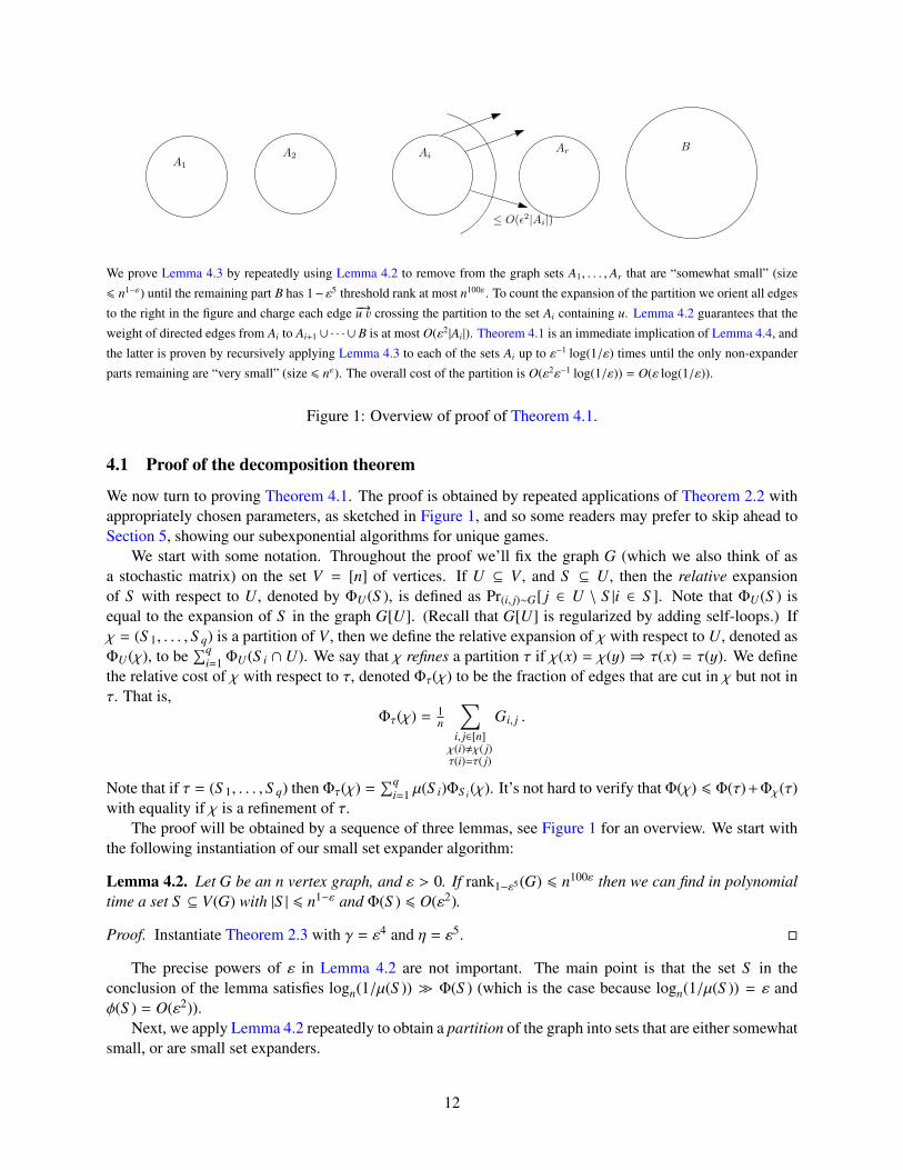
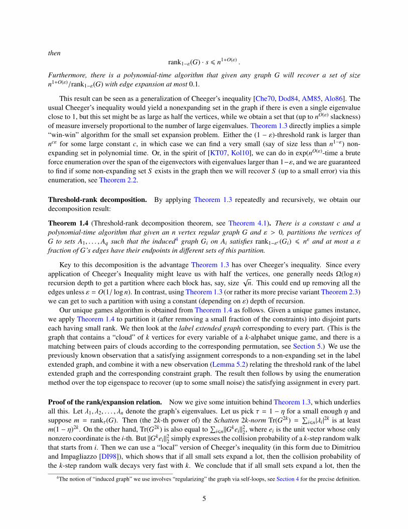
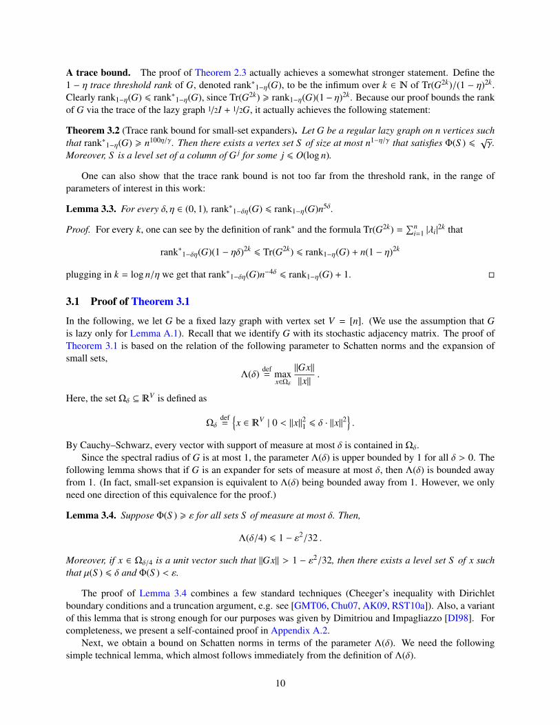
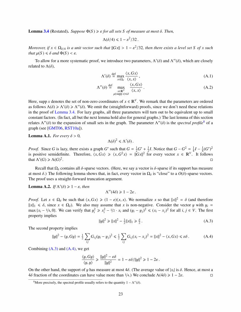
A1

A2 AiAr B

≤ O(ε2|Ai|)

We prove Lemma 4.3 by repeatedly using Lemma 4.2 to remove from the graph sets A1, . . . , Ar that are “somewhat small” (size

6 n1−ε) until the remaining part B has 1− ε5 threshold rank at most n100ε. To count the expansion of the partition we orient all edges

to the right in the figure and charge each edge −→u v crossing the partition to the set Ai containing u. Lemma 4.2 guarantees that the

weight of directed edges from Ai to Ai+1 ∪ · · · ∪ B is at most O(ε2|Ai|). Theorem 4.1 is an immediate implication of Lemma 4.4, and

the latter is proven by recursively applying Lemma 4.3 to each of the sets Ai up to ε−1 log(1/ε) times until the only non-expander

parts remaining are “very small” (size 6 nε). The overall cost of the partition is O(ε2ε−1 log(1/ε)) = O(ε log(1/ε)).

Figure 1: Overview of proof of Theorem 4.1.

4.1 Proof of the decomposition theorem

We now turn to proving Theorem 4.1. The proof is obtained by repeated applications of Theorem 2.2 withappropriately chosen parameters, as sketched in Figure 1, and so some readers may prefer to skip ahead toSection 5, showing our subexponential algorithms for unique games.

We start with some notation. Throughout the proof we’ll fix the graph G (which we also think of asa stochastic matrix) on the set V = [n] of vertices. If U ⊆ V , and S ⊆ U, then the relative expansionof S with respect to U, denoted by ΦU(S ), is defined as Pr(i, j)∼G[ j ∈ U \ S |i ∈ S ]. Note that ΦU(S ) isequal to the expansion of S in the graph G[U]. (Recall that G[U] is regularized by adding self-loops.) Ifχ = (S 1, . . . , S q) is a partition of V , then we define the relative expansion of χ with respect to U, denoted asΦU(χ), to be

∑qi=1 ΦU(S i ∩ U). We say that χ refines a partition τ if χ(x) = χ(y) ⇒ τ(x) = τ(y). We define

the relative cost of χ with respect to τ, denoted Φτ(χ) to be the fraction of edges that are cut in χ but not inτ. That is,

Φτ(χ) = 1n

∑i, j∈[n]χ(i),χ( j)τ(i)=τ( j)

Gi, j .

Note that if τ = (S 1, . . . , S q) then Φτ(χ) =∑q

i=1 µ(S i)ΦS i(χ). It’s not hard to verify that Φ(χ) 6 Φ(τ)+Φχ(τ)with equality if χ is a refinement of τ.

The proof will be obtained by a sequence of three lemmas, see Figure 1 for an overview. We start withthe following instantiation of our small set expander algorithm:

Lemma 4.2. Let G be an n vertex graph, and ε > 0. If rank1−ε5(G) 6 n100ε then we can find in polynomialtime a set S ⊆ V(G) with |S | 6 n1−ε and Φ(S ) 6 O(ε2).

Proof. Instantiate Theorem 2.3 with γ = ε4 and η = ε5.

The precise powers of ε in Lemma 4.2 are not important. The main point is that the set S in theconclusion of the lemma satisfies logn(1/µ(S )) Φ(S ) (which is the case because logn(1/µ(S )) = ε andφ(S ) = O(ε2)).

Next, we apply Lemma 4.2 repeatedly to obtain a partition of the graph into sets that are either somewhatsmall, or are small set expanders.

12

Lemma 4.3. There is a polynomial-time algorithm that given an n vertex graph G and ε > 0, out-puts a partition χ = (A1, . . . , Ar, B) of V(G), such that Φ(χ) 6 O(ε2), |Ai| 6 n1−ε for all i ∈ [r], andrank1−ε5(G[B]) 6 n100ε.

Proof. We start with an empty partition χ and will repeatedly add sets to χ until we cover V = V(G).Suppose we have already obtained the sets A1, . . . , Ai−1. Let Ui = V \ (A1∪· · ·∪Ai−1). We run the algorithmof Lemma 4.2 on G[Ui]. If it fails to return anything we add the set B = Ui to the partition and halt. (In thiscase, Lemma 4.2 guarantees that rank1−ε5(G[B]) 6 n100ε.) Otherwise, the algorithm returns a set Ai ⊆ Ui

with |Ai| 6 |Ui|1−ε 6 n1−ε and ΦUi(A) 6 O(ε2). We continue in this way until we have exhausted all of V .

Let χ = (A1, . . . , Ar, B) be the partition that we obtained in this way. Note that

Φ(χ) = 2r∑

i=1

G(Ai, Ai+1 ∪ · · · ∪ Ar ∪ B) = 2r∑

i=1

G(Ai,Ui \ Ai) .

But since G(Ai,Ui \ Ai) = Φ′U(Ai)µ(Ai) 6 O(ε2µ(Ai)), we can upper bound the cost of χ as desired

Φ(χ) 6 O(ε4r∑

i=1

µ(Ai)) 6 O(ε2).

(Since∑r

i=1 µ(Ai) = 1.)

The idea for the next lemma is to apply Lemma 4.3 recursively until we obtain a partition of the verticesinto sets Ai are very small (|Ai| nε) and sets Bi that are small-set expanders. To achieve the bound onthe size of the sets, it is enough to recurse up to depth O(log(1/ε)/ε). In each level of the recursion, wecut at most an O(ε2) fraction of edges. Hence, the total fraction of edges that we cut across all levels is atmost O(ε log(1/ε)). (For this argument, it was important that the algorithm of Lemma 4.2 outputs set withlogn(1/µ(S )) Φ(S ).)

Lemma 4.4. There is an algorithm that given an n vertex graph G, and ε > 0, outputs a partitionχ = (A1, . . . , Ar, B1, · · · , Br′) of [n], such that Φ(χ) 6 O(ε log(1/ε)), |Ai| 6 nε for all i ∈ [r], andrank1−ε5(G[B j]) 6 n100ε all j ∈ [r′].

Proof. We let χ0 be the trivial partition of one set (with Φ(χ0) = 0) and will continually refine the parti-tion using Lemma 4.3 until we reach the desired form. Now for i = 0, 1, . . . , 10 log(1/ε)/ε we repeat thefollowing steps. As long as χi does not satisfy the above form, then for every set A of χi that satisfiesrank1−ε5(G[A]) > n100ε > |A|100ε we run Lemma 4.3 to obtain a partition χA of A with ΦA(χA) 6 O(ε2).We then let χi+1 be the partition obtained by refining every such set A in χi according to χA. Note that wemaintain the invariant that in χi, every set A such that rank1−ε5(G[A]) > n100ε has size at most n(1−ε)i

. Thus,after 10 log(1/ε)/ε iterations every such set will have size at most nε. At the end we output the final partitionχ = χ10 log(1/ε)/ε. It just remains to bound Φ(χ). To do that it suffices to prove that Φ(χi+1) 6 Φ(χi) + O(ε2),since this implis Φ(χ) 6 O(ε2 · log(1/ε)/ε) = O(ε log(1/ε)). So we need to prove Φχi(χi+1) 6 O(ε2). Butindeed, if we let A1, . . . , Ar be the sets in χi that χi+1 refines, then one can see that

Φχi(χi+1) =

b∑j=1

µ(A j)ΦA j(χA j) 6 O(ε2) ,

where the last inequality follows from∑µ(A j) 6 1 and the guarantee ΦA(χA j) 6 O(ε2) provided by

Lemma 4.3.

Lemma 4.4 immediately implies Theorem 4.1

13

Trace rank bound. Note that by using Theorem 3.2 instead of Theorem 2.3, if we assume the originalgraph is lazy, then we can get a partition of small trace threshold-rank instead of threshold rank. (One justneeds to note that if G is lazy then G[A] is lazy as well for every subset A of G’s vertices.) Thus our proofactually yields the following theorem as well:

Theorem 4.5 (Low trace threshold rank decomposition theorem). There is a polynomial time algorithm thaton input a graph G and ε > 0, outputs a partition χ = (A1, . . . , Aq) of V(G) such that Φ(χ) 6 O(ε log(1/ε))and for every i ∈ [q],

rank∗1−ε5(G[Ai]) 6 n100ε .

5 A subexponential algorithm for U G

In this section we give a subexponential algorithm for unique games. A unique game of n variables andalphabet k is an n vertex graph G whose edges are labeled with permutations on the set [k], where theedge (i, j) labeled with π iff the edge ( j, i) is labeled with π−1. An assignment to the game is a stringy = (y1, . . . , yn) ∈ [k]n, and the value of y is the fraction of edges (i, j) for which y j = π(yi), where π is thelabel of (i, j). The value of the game G is the maximum value of y over all y ∈ [k]n. Khot’s Unique GamesConjecture [Kho02] states that for every ε > 0, there is a k, such that it is NP-hard to distinguish between agame on alphabet k that has value at least 1 − ε, and such a game of value at most ε. We now show that thisproblem can be solved in subexponential time:

Theorem 5.1 (Subexponential algorithm for unique games). There is an exp(knO(ε)) poly(n)-time algorithmthat on input a unique game G on n vertices and alphabet size k that has an assignment satisfying 1 − ε6 ofits constraints outputs an assignment satisfying 1 − O(ε log(1/ε)) of the constraints.

5.1 Proof of Theorem 5.1.

We now turn to the proof. We assume the unique game constraint graph is d-regular for some d— thisis without loss of generality (see Appendix A.1). For a unique game G, the label extended graph of G,denoted G, is a graph on nk vertices, where for i, j ∈ [n] and a, b ∈ [k] we place an edge between (i, a) and( j, b) iff there is an edge (i, j) in G labeled with a permutation π such that π(a) = b. That is, every vertexi ∈ V(G) corresponds to the “cloud” Ci := (i, 1), . . . , (i, k) in V(G). We say that S ⊆ V(G) is conflict freeif S intersects each cloud in at most one vertex. Note that a conflict free set S in G corresponds to a partialassignment f = fS for the game G (i.e., a partial function from V(G) to [k]). We define the value of a partialassignment f , denoted val( f ), to be 2/(nd) times the number of labeled edges (i, j, π) such that both f (i) andf ( j) are defined, and π( f (i)) = f ( j).

We say that a unique game is lazy if each vertex has half of its constraints as self loops with the identitypermutation. The following simple lemma will be quite useful for us:

Lemma 5.2. Suppose that G is lazy. Then rank∗1−η(G) 6 k · rank∗1−η(G).

Proof. Since rank∗1−η(G) = inftTr(G2t)/(1 − η)2t, this follows from the fact that Tr(Gt) 6 k Tr(Gt) for allt. The latter just follows because of the fact that if there is a length t walk in G from the vertex (i, a) backto itself then there must be a corresponding length t walk from i back to itself in G (and in fact one wherecomposing the corresponding permutation yields a permutation that has a as a fixed point). Thus everylength t walk in G corresponds to at most k such walks in G.

Combining this with Lemma 3.3 we get the following corollary:

Corollary 5.3. For every δ, η and n vertex constraint graph G on alphabet k, rank1−δη(G) 6 knηrank1−η(G).

14

Because of Lemma 5.2, we will find it convenient to use the trace threshold rank partitioning algorithmof Theorem 4.5. We note that we could have instead used Corollary 5.3 instead, at some quantitative loss tothe parameters. Our algorithm is as follows:

Input: Unique game G on n variables of alphabet k that has value at least 1 − ε6.

Operation: 1. Make G lazy by adding to every vertex self loops accounting to half the weight labeledwith the identity permutation.

2. Run the partition algorithm of Theorem 4.5 to obtain a partition χ = A1, . . . , Aq of the graph Gwith Φ(χ) 6 O(ε log(1/ε)) such that for every i, rank1−ε5rank∗(Ai) 6 n100ε.

3. Let A1, . . . , Aq be the corresponding partition of the label-extended graph G. Note that for allt ∈ [q], G[At] = ˆG[At] and hence by Lemma 5.2 rank1−ε5(G[Ai]) 6 rank∗1−ε5(G[Ai]) 6 kn100ε.

4. For every t = 1 . . . q do the following:

(a) Run the exp(rank1−ε5(G[At])-time enumeration algorithm of Theorem 2.2 on the graphG[At] to obtain a sequence of sets St.

(b) For every set S ∈ St, we compute an assignment fS to the vertices in At as follows: Forevery i ∈ At, if Ci ∩ S = ∅, then fS assigns an arbitrary label to the vertex i, if |Ci ∩ S | > 0,then fS assigns one of the labels in C ∩ S to the vertex i. Let ft be the assignment ofmaximum value, and assign the variables corresponding to vertices in At according to ft.(Note that since the sets A1, . . . , Aq are disjoint, every variable will be assigned at exactlyone label.)

We now turn to analyze the algorithm. We assume the game has an assignment fopt satisfying 1 − ε6 ofthe constraints. Note that fopt still has the same value, and in fact even somewhat better— 1 − ε6/2— afterwe make the graph lazy. Let χ = (A1, . . . , At) be the partition obtained by the algorithm in Step 2. SinceΦ(χ) 6 1/2, the assignment fopt satisfies at least 1 − 2(ε6/2) = 1 − ε6 of the constraints that are not cut by χ.Let µt be the measure of At (also equalling the measure of At), and let εt be the fraction of constraints in At

that are violated by fopt. We know that∑q

t=1 µtεt 6 2ε6.The following lemma implies that the algorithm will output an assignment satisfying at least 1 − O(ε)

fraction of the constraints:

Lemma 5.4. Every partial assignment ft satisfies all but a 20εt/η fraction of the constraints in At.

Proof. Let S opt be the subset of At corresponding to the assignment fopt. Note that |S opt| = |At| andΦAt

(S opt) 6 εt. Thus, the sequence St contains a set S that has symmetric difference with S opt at most8(εt/η)|At| (Theorem 2.2). Let S ′ be the subset of At corresponding to the assignment fS . The constructionof fS (and thus S ′) ensures that the symmetric difference between S ′ and S is at most the symmetric differ-ence between S and S opt. (In fact, the symmetric difference of S and S ′ is equal to

∑i∈At ||S ∩Ci|−1|.) Hence,

S ′ has symmetric difference with S opt at most 16(εt/η)|At|. In other words, fS agrees with fopt on all but a16εt/η fraction of the vertices in At. Thus fS violates at most εt + 16εt/η 6 20εt/η of the constraints in At.The lemma follows because we choose ft as the best assignment among all assignments fS for S ∈ St.

Lemma 5.4 implies that among the constraints not cut by χ, the assignment we output satisfies all but a∑t

µt · 20εt/η = (20/η)∑

u

µiεtO(ε6/ε5) = O(ε) fraction of constraints.

Since χ cuts at most O(ε log(1/ε)) fraction of the constraints, the correctness of the algorithm follows. Onejust has to note that any solution satisfying 1 − γ fraction of the lazy game’s constraints satisfies at least1 − 2γ fraction of the original game’s constraints.

15

6 Algorithmic results for some UG-hard problems.

Since the U G problem is reducible to a host of other problems, one would hope that our ideasmight apply to these problems. We show that this does work out for the M C problem, shown unique-games hard by [CKK+05]. For other problems such as M C, S C and V C someobstacles remain. However we are able to use our algorithm to solve interesting instances of these problemsin subexponential time, where by “interesting” we mean the kind of instances that arose in existing integral-ity gaps, or PCP-based hardness results. The reason is that these instances are highly expanding in subsetsof size o(n), which implies they have low threshold rank.

Very recently, [RST10b] showed that a hypothesis about the approximability of small-set expansion(studied in [RS10]) implies that several UG-hard problems, e.g. M C and S C are hard toapproximate even on small-set expanders. In particular, this hypothesis implies that for every small enoughε > 0, given a graph G, it is NP-hard to distinguish between the case that the M C value of G is at least1 − ε and the case that G’s M C value is at most 1 −Ω(

√ε) and ΦG(2−100/ε) > 1/2.

We show that this problem can be solved (even with M C value 1 − O(ε) in the NO case) in timeexp(nε

c) for some absolute constant c > 0.

6.1 Subexponential algorithm for M C

In an instance of M C, we are given a graph G with vertex set V and a set D of pairs of vertices(demand pairs). A (D-)multicut is a partition χ = S 1, . . . , S r of V such that none of the sets S i containsa demand pair in D. The goal is to find a multicut χ that minimize Φ(χ), the fraction of edges cut by thepartition.

Using the ideas in [SV09], a straight-forward (but somewhat tedious) adaptation of our algorithm forU G gives the following algorithm for M C.

Theorem 6.1. There exists a constant d > 1 and an exp(nε) poly(n)-time algorithm that given a multicutinstance with optimal value εd finds a solution with value ε. Here, d is an absolute constant.

The approximation guarantee of the M C algorithm above is incomparable with the O(log n)-approximation of Garg, Vazirani, and Yannakakis [GVY04]. For ε 1/ log n, the O(log n)-approximationgives better guarantees. If ε > 1/ log n, our algorithm gives the best known guarantees. (If the degrees ofthe demand pairs are small, better approximations are possible [SV09].)

An important special case of U G, called Γ-M 2-L, reduces to M C [SV09]. Thereduction in [SV09] has the feature that the blow-up of the instance is linear in the alphabet size of theΓ-M 2-L instance (in contrast to the usual UG-reductions using longcodes).

Combining this reduction with the above theorem, we get an algorithm for Γ-M 2-L. In contrast toTheorem 5.1, the algorithm for Γ-M 2-L has a non-trivial running time even for k = n.

Theorem 6.2 (Improved algorithm for Γ-M 2-L). There is an exp((kn)O(ε)) poly(n)-time algorithm thaton input a Γ-M 2-L instance G on n vertices and alphabet size k that has an assignment satisfying 1−εd

of its constraints outputs an assignment satisfying 1 − O(ε) of the constraints. Here, d > 1 is an absoluteconstant.

We give a rough sketch of Theorem 6.1. The details are deferred to the full version.

Proof Sketch for Theorem 6.1. Let η = ε5. We consider two cases. If rank1−η(G) > n100ε, then thereexists a set S with |S | 6 n1−ε and Φ(S ) 6 O(ε2) (Lemma 4.2). In this case, we recurse on the subgraphsG[S ] and G[V \ S ]. Otherwise, if rank1−η(G) 6 n100ε, we can enumerate all non-expanding subsets in timeexp(n100ε) poly(n). For every such set S , we prune it to a S ′ that doesn’t contain any demand pairs (using the

16

obvious greedy algorithm). Out of all such pruned sets S ′, we select the set S ∗ that has the small expansionin G. We can use S ∗ as one of the components of our multicut and recurse on the subgraph G[V \ S ∗]. Thisrecursive algorithm and its analysis is very similar to Theorem 4.1. An important difference is that the costsof the sets S ∗ are charged to the cost of the optimal M C solution.

6.2 M C, S C and V C on low threshold rank graphs

We now sketch how one can use the eigenspace enumeration method to give improved approximation guar-antees M C, S C and V C in time exponential in the threshold rank. One can thenoptimize the relation between expansion and threshold rank, as in Theorem 2.2, to obtain subexponentialalgorithms on small set expanders, although we defer these calculations to the final version of this work. Wefirst record the following variant of the enumeration result (Theorem 2.2):

Theorem 6.3 (Eigenspace enumeration revisited). There is an exp(rank1−η(G)) poly(n)-time algorithm thatgiven ε > 0 and an n vertex d-regular graph G containing a set S with G(S , S ) > 1 − ε, outputs a sequenceof sets, one of which has symmetric difference at most 16(ε/η)|S | with the set S .

In particular for ε < 0.01 and η = 1/2 the algorithm will output a list of sets containing a set S ′ suchthat |E(S ′, S ′)| > (1 − 17ε)|E|.

Proof sketch. The proof follows in the same way as Theorem 2.2, except that we use a vector with positiveand negative entries instead of the zero/non-zero characteristic vector used there. That is, we define χS (i) =

+1 if i ∈ S and χS (i) = −1 otherwise. Note that 〈χS ,GχS 〉 6 −1 + 2ε. We then use the same argument asbefore to show that χS must have large projection to the top eigenspace.

We now sketch our algorithms for M C, S C and V C on graphs with small rank:

Theorem 6.4. There is an absolute constant c and an algorithm that on input an n vertex regular graphG such that M C(G) > 1 − ε, runs in time exp(rank1−η(G)) poly(n) and produces a cut of size at most1 − cε/η.

Proof sketch. The maximum cut is a set S satisfying G(S , S ) > 1−ε, and we will use Theorem 6.3 to obtaina set S ′ of O(ε/η) symmetric difference from S .

Theorem 6.5. There is an absolute constant c and an algorithm that on input an n vertex regular graph Gsuch that with a set S of size in (n/3, 2n/3) such that ΦG(S ) 6 ε, runs in time exp(rank1−η(G)) poly(n) andproduces a set S ′ of size in (n/3, 2n/3) satisfying ΦG(S ) 6 cε/η.

Proof sketch. This is obtained by just using the enumeration of Theorem 2.2.

Theorem 6.6. There is an absolute constant c and an algorithm that on input an n vertex regular graph Gwith a vertex cover of size k, outputs a vertex cover of size (2 − cη)k in time exp(rank1−η(G)) poly(n).

Proof sketch. Since the graph is regular, we know that k 6 n/2, and so denote k = n(1/2 + ε) for some ε.Letting S be the vertex cover, this means that G(S , S ) > 1 − 2ε, and so we can find in the above time a setS ′ with symmetric difference at most (32ε/η)|S | from S . This means that after removing S ′ from the graph,we have a vertex cover of the remaining edges consisting of at most (32ε/η)|S | vertices, and by the simplegreedy algorithm we can find a vertex cover of at most (64ε/η)|S | vertices. This means we can always find avertex cover of size minn, k(1+64ε/η) or equivalently a factor minn/k, 1+64ε/η larger than the optimumk. Since k = 1/2 + ε one can see that the ε that will maximize this expression is roughly η/64, in which casewe’ll get 2 − O(η) approximation factor.

17

7 Threshold rank of hypercontractive graphs

Integrality gap examples for several problems use graphs defined using the noise operator on the unit sphere.We define the class of hypercontractive graphs that include such graphs, and show that they have low (i.e.,polylogarithmic) threshold rank. As a corollary we get an algorithm that certifies in quasipolynomial timethat a hypercontractive graph is indeed a small set expander.

A graph G with vertex set V is θ-hypercontractive if

∀x ∈ v. ‖Gx‖ 6 ‖x‖2−θ ,

where ‖x‖2−θ2−θ = Ei∈V x2−θi .

Lemma 7.1. If G is θ-hypercontractive, then Λ(δ) < δγ for some γ = Ω(θ), where Λ is the parameter definedin Section 3.1.

Proof. For every vector x ∈ V ,

‖Gx‖2−θ 6 Ei∈V

x2−θi

= Ei∈V

x2(1−θ)i · xθi

6(Ei∈V x2

i)1−θ·(Ei∈V xi

)1/θ (using Holder’s Inequality)

= ‖x‖2(1−θ)‖x‖θ1

Thus, for γ = θ/(2 − θ), we have ‖Gx‖ 6 ‖x‖1−γ‖x‖γ1. Every vector x ∈ Ωδ satisfies ‖x‖1 6√δ‖x‖. Hence,

for x ∈ Ωδ, we have ‖Gx‖ 6 δγ/2‖x‖, which proves that Λ(δ) 6 δγ/2.

Lemma 7.2 (Schatten norm bound for hypercontractive graphs). If G is θ-hypercontractive, then for all evenk,

Tr Gk 6 n(1−γ)k,

where γ = θ/(2 − θ).

Proof. In the proof of the previous lemma, we showed that ‖Gx‖ 6 ‖x‖1−γ‖x‖γ1. Let e1, . . . , en be thecanonical basis ofV . We normalize the vectors so that ‖ei‖1 = 1 and ‖ei‖ =

√n for all i ∈ V . We can easily

verify that for all j ∈ and i ∈ V ,

‖G jei‖ 6 ‖ei‖(1−γ) j

1 = n(1−γ) j/2 .

(Here, we use that ‖G jei‖1 = 1 for all j ∈ N and i ∈ V .) Then, for all even k

Tr Gk = Ei∈V〈ei,Gkei〉

= Ei∈V‖Gk/2ei‖

2

6 n(1−γ)k/2.

Lemma 7.3 (Threshold rank for hypercontractive graphs). If G is θ-hypercontractive, then

rank1/2(G) 6 (log n)γ .

Proof. Let m = rank1/2(G). By the previous lemma, we have

m 6 2k Tr Gk 6 2kn(1−γ)k/2.

If we choose k ≈ 2/γ · log log n, we get that m 6 (log n)γ.

18

8 Conclusions

The most important open question is of course whether our methods can be extended to yield an exp(no(1))-time algorithm for unique games, hence refuting the Unique Games Conjecture, and more generally what isthe true complexity of the unique games and small set expansion problems. We note that any quantitativeimprovement to the bounds of Theorem 2.3 would translate to an improvement in our algorithm for thesmall set expansion problem, and so it might result in refuting the stronger variant of the UGC proposed in[RS10]. Another open question is whether our techniques can yield subexponential algorithms with betterapproximation guarantees for unique-games hard problems such as V C, M C, S Con every instance.

Acknowledgements

We are very grateful to Assaf Naor, who first suggested in an intractability center meeting that the eigenvaluedistribution, and in particular Schatten norms, could be related to small set expansion, and gave us a copy ofthe manuscript [Nao04]. We thank Alexandra Kolla for giving us an early copy of the manuscript [Kol10].The authors also had a number of very fruitful conversations on this topic with several people includingMoritz Hardt, Thomas Holenstein, Russell Impagliazzo, Guy Kindler, William Matthews, Prasad Raghaven-dra, and Prasad Tetali.

References

[AIMS10] S. Arora, R. Impagliazzo, W. Matthews, and D. Steurer. Improved algorithms for unique gamesvia divide and conquer. Technical Report ECCC TR10-041, ECCC, 2010.

[AK09] N. Alon and B. Klartag. Economical toric spines via Cheeger’s inequality. J. Topol. Anal.,1(2):101–111, 2009.

[AKK+08] S. Arora, S. Khot, A. Kolla, D. Steurer, M. Tulsiani, and N. Vishnoi. Unique games on expand-ing constraints graphs are easy. In Proc. 40th STOC. ACM, 2008.

[Alo86] N. Alon. Eigenvalues and expanders. Combinatorica, 6(2):83–96, 1986.

[AM85] N. Alon and V. D. Milman. λ1, isoperimetric inequalities for graphs, and superconcentrators.J. Combin. Theory Ser. B, 38(1):73–88, 1985.

[Aus07] P. Austrin. Towards sharp inapproximability for any 2-CSP. In FOCS, pages 307–317, 2007.

[BHHS10] B. Barak, M. Hardt, T. Holenstein, and D. Steurer. Subsampling mathematical relaxations andaverage-case complexity, 2010. Manuscript.

[BJK00] A. Bulatov, P. Jeavons, and A. Krokhin. Classifying the complexity of constraints using finitealgebras. SIAM J. Comput, 34(3):720–742, 2005. Prelim version in ICALP ’00.

[Che70] J. Cheeger. A lower bound for the smallest eigenvalue of the Laplacian. In Problems in analysis(Papers dedicated to Salomon Bochner, 1969), pages 195–199. Princeton Univ. Press, 1970.

[Chu07] F. Chung. Random walks and local cuts in graphs. Linear Algebra Appl., 423(1):22–32, 2007.

19

[CKK+05] S. Chawla, R. Krauthgamer, R. Kumar, Y. Rabani, and D. Sivakumar. On the hardness of ap-proximating multicut and sparsest-cut. Computational Complexity, 15(2):94–114, 2006. Prelimversion in CCC 2005.

[CMM06a] M. Charikar, K. Makarychev, and Y. Makarychev. Near-optimal algorithms for unique games.In STOC, pages 205–214, 2006.

[CMM06b] E. Chlamtac, K. Makarychev, and Y. Makarychev. How to play unique games using embed-dings. In Proc. 47th FOCS, pages 687–696. Citeseer, 2006.

[CP05] C. Chekuri and M. Pal. A recursive greedy algorithm for walks in directed graphs. In Proc.FOCS, pages 245–253, 2005.

[DI98] T. Dimitriou and R. Impagliazzo. Go with the winners for graph bisection. In Proc 9th SODA,pages 510–520, 1998.

[Dod84] J. Dodziuk. Difference equations, isoperimetric inequality and transience of certain randomwalks. Trans. Amer. Math. Soc., 284(2):787–794, 1984.

[FK99] A. M. Frieze and R. Kannan. Quick approximation to matrices and applications. Combinator-ica, 19(2):175–220, 1999.

[FR04] U. Feige and D. Reichman. On systems of linear equations with two variables per equation.Proc. of RANDOM-APPROX, pages 117–127, 2004.

[GKL03] A. Gupta, R. Krauthgamer, and J. R. Lee. Bounded geometries, fractals, and low-distortionembeddings. In FOCS, pages 534–543, 2003.

[GMR08] V. Guruswami, R. Manokaran, and P. Raghavendra. Beating the random ordering is hard:Inapproximability of maximum acyclic subgraph. In FOCS, pages 573–582, 2008.

[GMT06] S. Goel, R. Montenegro, and P. Tetali. Mixing time bounds via the spectral profile. Electron.J. Probab., 11:no. 1, 1–26 (electronic), 2006.

[GT06] A. Gupta and K. Talwar. Approximating unique games. In Proc. 17th SODA, page 106. ACM,2006.

[GVY04] N. Garg, V. V. Vazirani, and M. Yannakakis. Multiway cuts in node weighted graphs. J.Algorithms, 50(1):49–61, 2004.

[Hås97] J. Håstad. Some optimal inapproximability results. J. ACM, 48(4):798–859, 2001. Prelimversion STOC ’97.

[HK03] E. Halperin and R. Krauthgamer. Polylogarithmic inapproximability. In Proc. STOC, page594. ACM, 2003.

[IPZ01] R. Impagliazzo, R. Paturi, and F. Zane. Which problems have strongly exponential complexity?Journal of Computer and System Sciences, 63(4):512–530, 2001.

[Kho02] S. Khot. On the power of unique 2-prover 1-round games. In Proceedings of 34th STOC, pages767–775, New York, 2002. ACM Press.

[KKMO07] S. Khot, G. Kindler, E. Mossel, and R. O’Donnell. Optimal inapproximability results forMAX-CUT and other 2-variable CSPs? SIAM J. Comput., 37(1):319–357, 2007.

20

[Kol10] A. Kolla. Spectral algorithms for unique games. In Proc. CCC, 2010. To appear.

[KR08] S. Khot and O. Regev. Vertex cover might be hard to approximate to within 2 − ε. J. Comput.Syst. Sci., 74(3):335–349, 2008.

[KS09a] S. Khot and R. Saket. SDP integrality gaps with local `1-embeddability. In FOCS, pages565–574, 2009.

[KS09b] G. Kun and M. Szegedy. A new line of attack on the dichotomy conjecture. In Proceedings ofthe 41st annual ACM symposium on Symposium on theory of computing, pages 725–734. ACMNew York, NY, USA, 2009.

[KT07] A. Kolla and M. Tulsiani. Playing random and expanding unique games. Unpublishedmanuscript available from A. Kolla’s webpage, to appear in journal version of [AKK+08],2007.

[KV05] S. Khot and N. K. Vishnoi. The unique games conjecture, integrality gap for cut problems andembeddability of negative type metrics into `1. In FOCS, pages 53–62, 2005.

[LL93] A. K. Lenstra and H. W. J. Lenstra. The Development of the Number Field Sieve. Springer-Verlag, 1993.

[LS93] N. Linial and M. E. Saks. Low diameter graph decompositions. Combinatorica, 13(4):441–454, 1993.

[Luk82] E. M. Luks. Isomorphism of graphs of bounded valence can be tested in polynomial time. J.Comput. Syst. Sci., 25(1):42–65, 1982.

[MNRS08] R. Manokaran, J. Naor, P. Raghavendra, and R. Schwartz. SDP gaps and UGC hardness formultiway cut, 0-extension, and metric labeling. In STOC, pages 11–20, 2008.

[MOO05] E. Mossel, R. O’Donnell, and K. Oleszkiewicz. Noise stability of functions with low influ-ences: Invariance and optimality. Annals of Mathematics, 101:101, 2008. Preliminary versionin FOCS ’05.

[MR08] D. Moshkovitz and R. Raz. Two query PCP with sub-constant error. In Proc. 49th FOCS,pages 314–323, 2008.

[Nao04] A. Naor. On the Banach space valued Azuma inequality and small set isoperimetry in Alon-Roichman graphs. Unpublished manuscript, 2004.

[PY88] C. Papadimitriou and M. Yannakakis. Optimization, approximation, and complexity classes.JCSS, 43(3):425–440, 1991. Prelim version in STOC 88.

[Rag08] P. Raghavendra. Optimal algorithms and inapproximability results for every csp? In Proc. 40thSTOC, pages 245–254. ACM, 2008.

[RS09] P. Raghavendra and D. Steurer. Integrality gaps for strong SDP relaxations of Unique Games.In FOCS, pages 575–585, 2009.

[RS10] P. Raghavendra and D. Steurer. Graph expansion and the unique games conjecture. In STOC,2010. To appear.

21

[RST10a] P. Raghavendra, D. Steurer, and P. Tetali. Approximations for the isoperimetric and spectralprofile of graphs and related parameters. In Proc. STOC. ACM, 2010.

[RST10b] P. Raghavendra, D. Steurer, and M. Tulsiani. Reductions between expansion problems.manuscript, 2010.

[SHI90] R. Stearns and H. Hunt III. Power indices and easier hard problems. Math. Syst. Theory,23(4):209–225, 1990.

[Ste10] D. Steurer. Fast SDP algorithms for constraint satisfaction problems. In SODA, 2010. Toappear.

[SV09] D. Steurer and N. Vishnoi. Connections between unique games and multicut. Technical ReportTR09-125, ECCC, 2009.

[Sze76] E. Szemeredi. Regular partitions of graphs. Problemes combinatoires et theorie des graphes,Orsay, 1976.

[Tre05] L. Trevisan. Approximation algorithms for unique games. In FOCS, pages 197–205, 2005.

A Appendix

A.1 Reductions to regular instances

We sketch here a reduction from the problem, for ε < γ, of distinguishing between a 1−e vs 1−γ satisfiableunique game G to the problem of distinguishing between a 1 − ε/10 vs 1 − γ/10 satisfiable unique gameG′ whose constraint graph is regular (i.e., every vertex is adjacent to the edges with the same total weight).The proof uses the standard expander-based construction originating from [PY88]. We replace each vertexv in G of degree d with a “cloud” of d new vertices, each connected to one of v’s original neighbors. Weplace an expander graph of some constant degree d0 on the vertices of the clouds, and set the weightsso that now every vertex in the graph has one outside edge, and d0 expander edges into its cloud. Weassume that the expander graph has the property that every set S with µ(S ) 6 1/2 satisfies Φ(S ) > 0.2. Wethen set the weights so that the total weight of the expander edges is 0.9 of the graph, and place equalityconstraints on these edges to obtain the game G′. Clearly, a 1−ε satisfying assignment in G corresponds to a0.9 + 0.1(1− ε) = 1− ε/10 satisfying assignment in G′ that assigns the same value to all vertices in the samecloud. Moreover, given an assignment y′ satisfying 1 − β fraction of G′ constraints, one can see that if wetransform y′ to y by assigning every cloud according to its most popular value, then we can only improve thefraction of constraints we satisfy. Indeed, consider a set S of vertices in a cloud that were originally givena value that was not the most popular one. Thus, µ(S ) 6 1/2 and hence Φ(S ) > 0.2. This implies that in theassignment y, S is involved in at least 0.9 · 0.2|S | weight of unsatisfied equality constraints. On the otherhand, in y′ the set S will satisfy all equality constraints and violate at most 0.1|S | of its other constraints.Summing up over all such S ’s we get that the weight of constraints changed from violated to satisfied whenmoving from y to y′ is at least as large than the weight of constraints changed from satisfied to violated. (Wemay be counting some constraints twice, but we had a factor of two slackness anyway.) Thus y′ still has atleast 1 − β value in G′, and hence translates into an assignment with 1 − 10β value in G.

A.2 Restricted eigenvalues and small-set expansion (Proof of Lemma 3.4)

In this section, we prove Lemma 3.4.

22

Lemma 3.4 (Restated). Suppose Φ(S ) > ε for all sets S of measure at most δ. Then,

Λ(δ/4) 6 1 − ε2/32 .

Moreover, if x ∈ Ωδ/4 is a unit vector such that ‖Gx‖ > 1 − ε2/32, then there exists a level set S of x suchthat µ(S ) 6 δ and Φ(S ) < ε.

To allow for a more systematic proof, we introduce two parameters, Λ′(δ) and Λ′′(δ), which are closelyrelated to Λ(δ),

Λ′(δ) def= max

x∈Ωδ

〈x,Gx〉〈x, x〉

, (A.1)

Λ′′(δ) def= max

x∈V

µ(supp x)6δ

〈x,Gx〉〈x, x〉

. (A.2)

Here, supp x denotes the set of non-zero coordinates of x ∈ V . We remark that the parameters are orderedas follows Λ(δ) > Λ′(δ) > Λ′′(δ). We omit the (straightforward) proofs, since we don’t need these relationsin the proof of Lemma 3.4. For lazy graphs, all three parameters will turn out to be equivalent up to smallconstant factors. (In fact, all but the next lemma hold also for general graphs.) The last lemma of this sectionrelates Λ′′(δ) to the expansion of small sets in the graph. The parameter Λ′′(δ) is the spectral profile8 of agraph (see [GMT06, RST10a]).

Lemma A.1. For every δ > 0,Λ(δ)2 6 Λ′(δ) .

Proof. Since G is lazy, there exists a graph G′ such that G = 12G′ + 1

2 I. Notice that G − G2 = 14 I − 1

4 (G′)2

is positive semidefinite. Therefore, 〈x,Gx〉 > 〈x,G2x〉 = ‖Gx‖2 for every vector x ∈ V . It followsthat Λ′(G) > Λ(G)2.

Recall that Ωδ contains all δ-sparse vectors. (Here, we say a vector is δ-sparse if its support has measureat most δ.) The following lemma shows that, in fact, every vector in Ωδ is “close” to a O(δ)-sparse vectors.The proof uses a straight-forward truncation argument.

Lemma A.2. If Λ′(δ) > 1 − ε, thenΛ′′(4δ) > 1 − 2ε .

Proof. Let x ∈ Ωδ be such that 〈x,Gx〉 > (1 − ε)〈x, x〉. We normalize x so that ‖x‖2 = δ (and therefore‖x‖1 6 δ, since x ∈ Ωδ). We also may assume that x is non-negative. Consider the vector y with yi =

max xi − 1/4, 0. We can verify that y2i > x2

i −1/2 · xi and (yi − y j)2 6 (xi − x j)2 for all i, j ∈ V . The first

property implies‖y‖2 > ‖x‖2 − 1

2‖x‖1 >δ2 . (A.3)

The second property implies

‖y‖2 − 〈y,Gy〉 = 12

∑i j

Gi j(yi − y j)2 6 12

∑i j

Gi j(xi − x j)2 = ‖x‖2 − 〈x,Gx〉 6 εδ . (A.4)

Combining (A.3) and (A.4), we get

〈y,Gy〉〈y, y〉

>‖y‖2 − εδ

‖y‖2= 1 − εδ/‖y‖2 > 1 − 2ε .

On the other hand, the support of y has measure at most 4δ. (The average value of |xi| is δ. Hence, at most a4δ fraction of the coordinates can have value more than 1/4.) We conclude Λ(4δ) > 1 − 2ε.

8More precisely, the spectral profile usually refers to the quantity 1 − Λ′′(δ).

23

The following relation between Λ′′(δ) and the expansion of small sets in G is a direct consequence ofthe proof of Cheeger’s inequality [AM85, Alo86] (see for example [GMT06, Chu07, AK09]).

Lemma A.3. Suppose Λ′′(δ) > 1 − ε. Then, there exists a vertex set S with µ(S ) 6 δ and

Φ(S ) 6√

8ε .

Proof. By the definition of Λ′′(δ), there exists a δ-sparse vector such that 〈x,Gx〉 > (1− ε)〈x, x〉. By scalingand taking absolute values, we may assume that all coordinates of x satisfy 0 6 xi 6 1. We considerthe following distribution over vertex sets S : Sample a random threshold t ∈ [0, 1] and output the setS t := i ∈ V | x2

i > t. This distribution over vertex sets has the following properties:

Et∈[0,1]

µ(S t) = 〈x, x〉 , (A.5)

Et∈[0,1]

〈1S t ,G1V\S t〉 = Ei∈V

∑j

Gi j|x2i − x2

j | . (A.6)

By Cauchy–Schwarz, we can upper bound the latter expectation as follows

Ei∈V

∑j

Gi j|x2i − x2

j | 6(

Ei∈V

∑jGi j(xi − x j)2

)1/2·(

Ei∈V

∑jGi j(xi + x j)2

)1/2

=(2〈x, x〉 − 2〈x,Gx〉

)1/2·(2〈x, x〉 + 2〈x,Gx〉

)1/2

6 2√

2(〈x, x〉 − 〈x,Gx〉

)1/2· 〈x, x〉1/2 6 2

√2 ·√ε · 〈x, x〉 .

It follows that there exists a threshold t∗ such that

Φ(S t∗) =〈1S t∗ ,G1V\S t∗ 〉

µ(S t)6

Et∈[0,1]〈1S t ,G1V\S t〉

Et∈[0,1] µ(S t)6 2√

2 ·√ε .

On the other hand, every set S t is a subset of the support of x and thus µ(S t∗) 6 δ as desired.

We can prove Lemma 3.4 by combining the previous lemmas: Suppose that Φ(S ) > ε for all S withµ(S ) 6 δ. Then, we have Λ′′(δ) 6 1 − ε2/8 (Lemma A.3), Λ′(δ/4) 6 1 − ε2/16 (Lemma A.2) and soΛ(δ/3) 6

√1 − ε2/16 6 1 − ε2/32 (Lemma A.1). Moreover, following the proof of these lemmas, we see

that they allow us to obtain from a vector x ∈ Ωδ/4 satisfying ‖Gx‖2 > (1 − ε2/32)‖x‖2 a set S of measureat most δ satisfying Φ(S ) 6 ε, and moreover the set S is obtained as a level set of the vector y whereyi = maxxi − 1/4, 0, or equivalently, a level set of x.

24