Embed Size (px)
Citation preview
Submitted to the Annals of Applied Statistics
FULL MATCHING APPROACH TO INSTRUMENTALVARIABLES ESTIMATION WITH APPLICATION TO THE
EFFECT OF MALARIA ON STUNTING
By Hyunseung Kang∗ Benno Kreuels†,‡ Jurgen May‡ and DylanS. Small∗
University of Pennsylvania∗, University Medical Centre† and BernhardNocht Institute for Tropical Medicine‡
Most previous studies of the causal relationship between malariaand stunting have been studies where potential confounders are con-trolled via regression-based methods, but these studies may have beenbiased by unobserved confounders. Instrumental variables (IV) re-gression offers a way to control for unmeasured confounders where,in our case, the sickle cell trait can be used as an instrument. How-ever, for the instrument to be valid, it may still be important toaccount for measured confounders. The most commonly used instru-mental variable regression method, two-stage least squares, relies onparametric assumptions on the effects of measured confounders toaccount for them. Additionally, two-stage least squares lacks trans-parency with respect to covariate balance and weighing of subjectsand does not blind the researcher to the outcome data. To addressthese drawbacks, we propose an alternative method for IV estimationbased on full matching. We evaluate our new procedure on simulateddata and real data concerning the causal effect of malaria on stuntingamong children. We estimate that the risk of stunting among childrenwith the sickle cell trait decreases by 0.22 per every malaria episodeprevented by the sickle cell trait, a substantial effect of malaria onstunting (p-value: 0.011, 95% CI: 0.044, 1).
1. Introduction.
1.1. Motivation: Does malaria cause stunting?. From January 2003 toJanuary 2004, 1070 infants from Ghana, Africa were recruited to a clini-cal trial on Intermittent Preventative Treatment for malaria (IPT) (Kobbeet al., 2007). From the time of recruitment at 3 months of age until twoyears of age, each child was monitored monthly for the presence of malariaparasites with measurements every three months of length/height. Table 1lists the baseline characteristics of the 1070 infants in our data.
Keywords and phrases: Full matching, Instrumental variables, Malaria, Stunting, Two-stage least squares
1imsart-aoas ver. 2014/10/16 file: mainText-Revision2.tex date: November 11, 2015
arX
iv:1
411.
7342
v4 [
stat
.AP]
10
Nov
201
5
2 H. KANG ET AL.
One of the public health questions of interest from this clinical study waswhether malaria caused stunted growth among children. In 2013 alone, therewere 128 million estimated cases of malaria in sub-Saharan Africa, with mostcases occurring in children under the age of 5 (World Health Organization,2014). Stunting, defined as a child’s height being two standard deviationsbelow the mean for his/her age, is a key indicator of child development(WHO Multicentre Growth Reference Study Group, 2006). If malaria doescause stunted growth, several intervention strategies can be implementedto mitigate stunted growth, such as distribution of mosquito nets, controlof the mosquito population during seasons of high malarial incidence, andsurveillance of mosquito populations.
The current body of evidence suggests that there is a strong positive rela-tionship between malaria exposure and stunted growth (Genton et al., 1998;Deen, Walraven and von Seidlein, 2002; Nyakeriga et al., 2004; Ehrhardtet al., 2006; Fillol et al., 2009; Deribew et al., 2010; Crookston et al., 2010).Unfortunately, a fundamental limitation with these prior studies is that theyare observational studies and consequently, there is always a concern thatimportant confounders were not controlled for. For example, Fillol et al.(2009) and Deribew et al. (2010) stated that a limitation in their studieswas not controlling for diet, specifically a child’s intake of micronutrientssuch as vitamins, zinc, or iron as these micronutrients could impact a child’sgrowth as well as his immune system’s ability to fight off a malaria episode.In addition, Ehrhardt et al. (2006) and Crookston et al. (2010) suggestedcontrolling for socioeconomic factors in future studies of malaria and malnu-trition because affluent families are more likely to provide mosquito nets andnutritious food to their children compared to impoverished families. Shortof a randomized clinical trial, which is unethical in this context, unmeasuredconfounders are likely present in all the aforementioned studies, because ofthe practical limitations of accounting for all possible confounders.
1.2. Instrumental variables and sickle cell trait. Instrumental variables(IVs) is an alternative method to estimate the causal effect of an exposure onthe outcome when there is unmeasured confounding, provided that a valid in-strument is available (Angrist, Imbens and Rubin, 1996; Hernan and Robins,2006; Brookhart and Schneeweiss, 2007; Cheng, Qin and Zhang, 2009; Swan-son and Hernan, 2013; Baiocchi, Cheng and Small, 2014). The core assump-tions for a variable to be a valid instrumental variable are that the variable(A1) is associated with the exposure, (A2) has no direct pathways to theoutcome, and (A3) is not associated with any unmeasured confounders aftercontrolling for the measured confounders (See Figure 1 and Section 2.3 for
imsart-aoas ver. 2014/10/16 file: mainText-Revision2.tex date: November 11, 2015

FULL MATCHING IV ESTIMATION 3
Fig 1. Causal diagram for the malaria study. Numbers (A1,A2,A3) represent MR assump-tions.
more detailed discussions). If measured covariates are available, like in ourdata, the plausibility of the instrument satisfying the three core assumptionscan be improved by conditioning on the covariates, especially (A3). For ourstudy of analyzing the causal effect of malaria on stunting, we follow a recentapproach by Davey Smith and Ebrahim (2003) and especially Kang et al.(2013) where genotypic variations are used as instruments and propose touse the presence of a sickle cell genotype (HbAS) versus carrying the normalhemoglobin type (HbAA) as an instrument. The sickle cell genotype (HbAS)is a condition where a person inherits from one parent a mutated copy ofthe hemoglobin beta (HBB) gene called the sickle cell gene mutation thatbends red blood cells into a sickle (crescent) shape, but inherits a normalcopy of the HBB gene from the other parent. The sickle cell trait protectsagainst malaria, but is thought to be otherwise mostly asymptomatic (Aidooet al., 2002). Note that we exclude from the analysis people who have twocopies of the HBB gene, i.e. people who suffer from sickle cell disease whichcauses severe symptoms; sickle cell disease (two copies of the HBB gene) isthought to persist despite its evolutionary disadvantage because of the sicklecell trait (one copy of the HBB gene) protecting against malaria (May et al.,2007). We discuss in detail the validity of the sickle cell trait IV in Section2.3. In addition, we propose to combine the covariates that were alreadymeasured for this data in Table 1 to increase the plausibility of our sicklecell trait being a valid instrument.
imsart-aoas ver. 2014/10/16 file: mainText-Revision2.tex date: November 11, 2015

4 H. KANG ET AL.
1.3. Two-stage least squares. The most popular and well-studied amongmethods that use an IV and measured covariates to estimate causal effectsis two-stage least squares (2SLS) (Angrist and Krueger, 1991; Card, 1995;Wooldridge, 2010). For example, in Card (1995), which studied the effectof education on wages, 2SLS with proximity to a 4-year college as an IVwas used to control for measured covariates such as race and parents’ ed-ucation. Specifically, 2SLS first estimated, via least squares, the predictedexposure (education) given the instrument (proximity to 4-year college) andthe measured covariates, and second, regressed the outcome (earnings) onthis predicted exposure and the measured covariates; the 2SLS estimate ofthe causal effect is the coefficient on the predicted exposure in the secondregression. Standard results in econometrics show 2SLS estimators are con-sistent and efficient under linear single-variable structural equation modelswith a constant treatment effect (Wooldridge, 2010). When treatment ef-fects are not constant, Angrist and Imbens (1995) showed that under cer-tain monotonicity assumptions, 2SLS converges to a weighted average of thecovariate-specific treatment effects with the weights proportional to the av-erage conditional variance of the expected value of the treatment given thecovariates and the instrument. Other IV methods to estimate causal effectsin the presence of measured covariates include Bayesian methods (Imbensand Rubin, 1997), semiparametric methods (Abadie, 2003; Tan, 2006; Og-burn, Rotnitzky and Robins, 2015), and nonparametric methods (Frolich,2007).
Despite its attractive estimation properties, 2SLS has some drawbacksin (i) lack of transparency of the population to which the estimate applies,(ii) lack of blinding of the analyst/researcher and (iii) dependence on para-metric assumptions. First, with regards to transparency, suppose that thereare some values of the covariates for which the instrument is almost alwayslow, some values for which the instrument is almost always high and somevalues of the covariates for which the instrument takes on both low and highvalues. Then, the 2SLS estimate will put most of its weight on the causaleffect for subjects with the values of the covariates for which the instru-ment takes on both low and high values, and little weight on subjects withthe values of the covariates for which the instrument usually takes on low(or high) values. In our malaria study, this would mean that there mightbe some villages (a covariate) that are receiving little weight in the 2SLSestimate; consequently, the 2SLS estimate might not be helpful for under-standing the effect of malaria on stunting in these villages even though thesevillages might have contributed many subjects to the analysis. Although theweighting function in 2SLS can be studied, there is nothing in the 2SLS es-
imsart-aoas ver. 2014/10/16 file: mainText-Revision2.tex date: November 11, 2015

FULL MATCHING IV ESTIMATION 5
timation procedure itself that warns us when some values of the covariatesare receiving little weight and it is rare to see discussion of the weightingfunction for 2SLS in empirical papers.
Second, 2SLS lacks blinding with respect to the outcome data when ad-justing for covariates. Cochran (1965), Rubin (2007) and Rosenbaum (2010)argue that the best observational studies resemble randomized experiments.An important feature of the design of randomized experiments is that whendesigning the study and planning the analysis, the researcher is blinded tothe outcome data. However, in regression-based procedures for adjustingfor covariates like 2SLS, there is often judgment that needs to be exercisedin choosing covariate adjustment models, which require one to look at theoutcome data and estimates of causal effects to exercise such judgment. Itis difficult even for the most honest researcher to be completely objectivein comparing models when the researcher has an a priori hypothesis or ex-pectation about the direction of the causal effect (Rubin and Waterman,2006).
Third, 2SLS relies on proper specification of how the measured covariatesaffect the outcomes. Often, parametric modeling assumptions are made forhow the measured confounders affect the outcome. In particular, 2SLS, asusually implemented, relies on the measured confounders having a linear ef-fect on the expected outcome. Section 3.1 contains simulation evidence about2SLS that demonstrates its reliance on linear, parametric assumptions.
1.4. Instrumental variables with full matching. Matching is an alterna-tive method to adjust for measured covariates. A matching algorithm groupsindividuals in the data with different values of the instrument but similarvalues of the observed covariates, so that within each group, the only dif-ference between the individuals is their values of the instrument (Haviland,Nagin and Rosenbaum, 2007; Rosenbaum, 2010; Stuart, 2010). For example,in the malaria data, a matching algorithm seeks to produce matched sets sothat in a matched set, individuals are born in the same village and are sim-ilar on other measured covariates. The only difference between individualsin a matched set is their instrument values. We can then compare stunt-ing between individuals with high and low values of the instrument withina matched set to assess the effect of malaria on stunting (Baiocchi et al.,2010).
Matching addresses the drawbacks of 2SLS discussed in the previous sec-tion. First, if there are values of covariates for which almost all subjectshave a high (or low) value of the IV, then the matching algorithm and as-sociated diagnostics will tell us that matched sets cannot be formed when
imsart-aoas ver. 2014/10/16 file: mainText-Revision2.tex date: November 11, 2015

6 H. KANG ET AL.
subjects in the matched sets have certain values of the covariates but dif-ferent levels of the IV; thus, it will be transparent that for these values ofthe covariates, the causal effect cannot be estimated without extrapolation.Relatedly, matching allows us to control the weighting of subjects with dif-ferent values of the covariates to make the weighting transparent, such asweighting the covariates in proportion to their population frequency. Second,matching is blind to the outcome data; a matching algorithm only requiresthe measured covariates and the instrument values for each individual inthe data. Diagnostics can be done and the matching can be adjusted untilit is adequate, all without looking at the outcome data. Finally, when esti-mating the causal effect, matching makes non-parametric inference; it doesnot use any parametric assumptions model such as linearity and parametricassumptions on the model.
Previous work using matching in studying causality is abundant in non-IV settings; see Stuart (2010) for a complete overview. In contrast, workon using matching methods on IV estimation is limited to pair matching(Baiocchi et al., 2010) and fixed control matching, i.e. each unit with level1 of the IV is matched to a fixed number of units with level 0 of the IV(Kang et al., 2013). A drawback to these matching methods is that they donot use the full data (Keele and Morgan, 2013; Zubizarreta et al., 2013).In particular, Kang et al. (2013) studied the same causal effect of interest,malaria on stunting, but with a smaller amount of data, because the statis-tical methodology was limited to matching with fixed controls. That is, outof the total of 884 individuals available, the matching algorithm dropped25% of the individuals and the final statistical inference was based only on660 individuals.
In this paper, we develop an IV full matching approach that uses the fulldata. Full matching is the most general, flexible, and optimal type of match-ing (Rosenbaum, 1991; Hansen, 2004; Rosenbaum, 2010). Specifically, fullmatching is the generalization of any type of matching, such as pair match-ing, matching with fixed controls, or matching with variable controls. Fullmatching is also flexible in that it can incorporate constraints on matchedset structures, such as limiting the number of individuals in each matchedset, to improve statistical efficiency. Finally, full matching is optimal in thesense that it produces matched sets where within each set, measured covari-ates between individuals with different instrument values are most similar(Rosenbaum, 1991).
Under IV estimation with full matching, we derive a randomization-basedtesting procedure and sensitivity analysis based on the proposed test statis-tic. We conduct simulation studies to study the performance of 2SLS versus
imsart-aoas ver. 2014/10/16 file: mainText-Revision2.tex date: November 11, 2015
FULL MATCHING IV ESTIMATION 7
full matching IV estimation, specifically analyzing the robustness of bothmethods to non-linearity (Section 3.1). In the same spirit, we also conductsimulation studies to compare our full matching IV estimation with anothernonparametric method introduced by (Frolich, 2007) introduced in Section1.3, specifically looking at bias and variance between the two nonparametricmethods. Finally, we apply full matching IV estimation to analyze the causaleffect of malaria on stunting and demonstrate the full matching method’stransparency in adjusting for covariates.
2. Methods.
2.1. Notation. To introduce the idea of matching in IV estimation, weintroduce the following notation. Let i = 1, . . . , I index the I total matchedsets that individuals are matched into. Each matched set i contains ni ≥ 2subjects who are indexed by j = 1, . . . , ni and there are a total of N =∑I
i=1 ni individuals in the data. Let Zij denote a binary instrument forsubject j in matched set i. In each matched set i, there are mi subjects withZij = 1 and ni−mi subjects with Zij = 0. For instance, in the malaria data,for each ith matched set, there are mi children who inherited the sickle celltrait, HbAS (i.e. Zij = 1), and ni −mi children who inherited HbAA (i.e.Zij = 0). Let Z be a random variable that consists of the collection of Zij ’s,Z = (Z11, Z12, ...., ZI,nI
). Define Ω as the set that contains all possible valuesz of Z, so z ∈ Ω if zij is binary and
∑nij=1 zij = mi for all I matched sets.
Thus, the cardinality of Ω, denoted as |Ω|, is |Ω| =∏Ii=1
(nimi
). Denote Z to
be the event that Z ∈ Ω.For individual j in matched set i, define d1ij and d0ij to be the potential
exposure values under Zij = 1 or Zij = 0, respectively. With the malariadata, d1ij and d0ij represent the number of malaria episodes the child wouldhave if she had the sickle cell trait, Zij = 1, and no sickle cell trait, Zij = 0,
respectively. Also, define r(k)1ij to be the outcome individual i would have if
she were assigned instrument value 1 and level k of the exposure, and r(k)0ij
to be the outcome individual i would have if she were assigned instrumental
value 0 and level k of the exposure. Then, r(d1ij)1ij and r
(d0ij)0ij are the potential
outcomes if the individual were assigned levels 1 and 0 of the instrumentrespectively and the exposure took its natural level given the instrument,
resulting in exposures, d1ij and d0ij , respectively. In the malaria data, r(d1ij)1ij
is a binary variable that represents whether the jth child in the ith matchedset would be stunted (i.e. 1) or not (i.e. 0) if the child carried the sickle
cell trait (i.e. if Zij = 1) and r(d0ij)0ij is a binary variable that represents
whether the child would be stunted or not if the child carried no sickle cell
imsart-aoas ver. 2014/10/16 file: mainText-Revision2.tex date: November 11, 2015

8 H. KANG ET AL.
trait (i.e. if Zij = 0). The potential outcome notations assume the StableUnit Treatment Value Assumption where (i) an individual’s outcome andexposure depend only on her own value of the instrument and not on otherpeople’s instrument values and (ii) an individual’s outcome only depends onher own value of the exposure and not on other people’s exposure (Rubin,1980).
For individual j in matched set i, let Rij be the binary observed outcome
and Dij be the observed exposure. The potential outcomes r(d1ij)1ij , r
(d0ij)0ij , d1ij ,
and d0ij and the observed values Rij , Dij , and Zij are related by the followingequation:
(1) Rij = r(d1ij)1ij Zij + r
(d0ij)0ij (1− Zij) Dij = d1ijZij + d0ij(1− Zij)
For individual j in matched set i, let Xij be a vector of observed covariatesand uij be the unobserved covariates. For example, in the malaria data, Xij
represents each child’s covariates listed in Table 1 while uij is an unmeasuredconfounder, like diet, which was mentioned in Section 1.1. We define the set
F = (r(d1ij)1ij , r
(d0ij)0ij , d1ij , d0ij ,Xij , uij), i = 1, ..., I, j = 1, ..., ni to be the
collection of potential outcomes and all covariates/confounders, observedand unobserved.
2.2. Full matching algorithm. A matching algorithm controls the biasresulting from different observed covariates by creating I matched sets in-dexed by i, i = 1, . . . , I such that individuals within each matched set havesimilar covariate values xij and the only difference between individuals ineach matched set is their instrument values, Zij . In a full matching algo-rithm, each matched set i either contains mi = 1 individual with Zij = 1and ni − 1 individuals with Zij = 0 or mi = ni − 1 individuals with Zij = 1and 1 individual with Zij = 0.
Rosenbaum (2002, 2010), Hansen (2004), and Stuart (2010) provide anoverview of matching and a discussion on various distance metrics and toolsto measure similarity for observed and missing covariates. For the malariadata, Section 4.2 describes how we used propensity score caliper matchingwith rank-based Mahalanobis distance to measure covariate similarity. Oncewe have obtained the distance matrix, we use an R package available onCRAN called optmatch developed by Hansen and Klopfer (2006) to find theoptimal full matching.
2.3. Conditions for sickle cell trait as a valid instrument. We formal-ize the core assumptions of an instrumental variable below (Holland, 1988;Angrist, Imbens and Rubin, 1996; Yang et al., 2014) (see Figure 1).
imsart-aoas ver. 2014/10/16 file: mainText-Revision2.tex date: November 11, 2015

FULL MATCHING IV ESTIMATION 9
(A1) The instrument must be associated with the exposure, or in F ,∑I
i=1∑nij=1(d1ij − d0ij) 6= 0
(A2) The instrument can only affect the outcome if it affects the exposure.
Since the r’s don’t depend on z under this assumption, we write r(k)1ij =
r(k)0ij ≡ r
(k)ij for all k in F (exclusion restriction)
(A3) The instrument is effectively randomly assigned within a matched set,P (Zij = 1|F ,Z) = mi/ni for each i.
In Figure 1, (A1) corresponds to there being an association between theinstrument and the exposure, (A2) corresponds to that all directed path-ways from the instrument to the outcome pass through the exposure and(A3) corresponds to the instrument, conditional on measured variables, be-ing unassociated with unmeasured variables that are associated with theoutcome.
We now assess the validity of (A1)-(A3) for the sickle cell trait, the instru-ment for our analysis on the effect of malaria on stunting. For assumption(A1), there is substantial evidence that the sickle cell trait does provide pro-tection against malaria as compared to people with two normal copies of theHBB gene (HbAA) (Aidoo et al., 2002; Williams et al., 2005; May et al.,2007; Cholera et al., 2008; Kreuels et al., 2010). For assumption (A2), thiscould be violated if the sickle cell trait had effects on stunting other thanthrough causing malaria, for instance, if the sickle cell trait was pleiotropic(Davey Smith and Ebrahim, 2003). We can partially test this assumption byexamining individuals who carry the sickle cell trait, but who grew up in a re-gion where malaria is not present. That is, if assumption (A2) were violated,heights between individuals with HbAS and HbAA in such a region would bedifferent since there would be a direct arrow between the sickle cell trait andheight. We examined studies among African American children and childrenfrom the Dominican Republic and Jamaica for whom the sickle cell trait iscommon, but there is no malaria in the area. These two regions also matchnutritional and socioeconomic conditions that are closer to our study pop-ulation in Ghana so that the populations (and subsequent subpopulationsamong them) are comparable. From these studies from the regions, we foundno evidence that the sickle cell trait affected a child’s physical development(Ashcroft, Desai and Richardson, 1976; Kramer, Rooks and Pearson, 1978;Ashcroft et al., 1978; Rehan, 1981). This supports the validity of assumption(A2).
Although the results of this test support the validity of (A2), (A2) couldstill be violated. For example, the regions we use to support assumption (A2)may be different than Ghana through unmeasured characteristics, which
imsart-aoas ver. 2014/10/16 file: mainText-Revision2.tex date: November 11, 2015
10 H. KANG ET AL.
would make the populations incomparable. As another example, the sicklecell trait could have a direct effect that interacts with the environment insuch a way that the direct effect is only present in Africa, but not in theUnited States, the Dominican Republic, or Jamaica. One specific point ofconcern raised by a referee is iron supplements. In the malaria study thatwe are considering, children with low hemoglobin received iron supplementsand iron supplements can reduce the risk of stunting. A potential concern isthat the sickle cell trait may induce a child to have low iron levels, therebyincreasing the risk of stunting without going through the malaria pathwayin Figure 1 and violating (A2). However, Kreuels et al. (2010) found thatin the malaria study we are considering, children carrying HbAA tend tohave lower hemoglobin levels than children carrying HbAS. Thus, childrenwith the sickle cell trait, HbAS, were less likely to receive iron supplements.Consequently, if there’s a violation of the exclusion restriction because of ironsupplements, it would tend to bias our estimate of the increase in stuntingfrom malaria downwards and our estimate can be regarded as a conservativeestimate of the effect of malaria on increasing stunting.
For assumption (A3), this assumption would be questionable in our dataif we did not control for any population stratification covariates. Populationstratification is a condition where there are subpopulations, some of whichare more likely to have the sickle cell trait, and some of which are morelikely to be stunted through mechanisms other than malaria (Davey Smithand Ebrahim, 2003). For example, in Table 1 which provides the baselinecharacteristics for our data, we observed that the village Tano-Odumasi hadmore children with HbAA than HbAS. It is possible that there are othervariables besides HbAA that differ between the village Tano-Odumasi andother villages and affect stunting. Hence, assumption (A3) is more plausibleif we control for observed variables like village of birth. Specifically, withinthe framework of full matching, for each matched set i, if the observed vari-ables xij are similar among all ni individuals, it may be more plausible thatthe unobserved variable uij plays no role in the distribution of Zij amongthe ni children. If (A3) exactly holds and subjects are exactly matched forXij , then within each matched set i, Zij is simply a result of random assign-ment where Zij = 1 with probability mi/ni and Zij = 0 with probability(ni −mi)/ni when we condition on the number of units int he matched setwith Zij = 1 being mi. In Section D, we discuss a sensitivity analysis thatallows for the possibility that even after matching for observed variables,the unobserved variable uij may still influence the assignment of Zij in eachmatched set i, meaning that assumption (A3) is violated.
imsart-aoas ver. 2014/10/16 file: mainText-Revision2.tex date: November 11, 2015
FULL MATCHING IV ESTIMATION 11
There are also other assumptions associated with instrumental variables,most notably the Stable Unit Treatment Value Assumption (SUTVA) inSection 2.1 and the monotonicity assumption in Angrist, Imbens and Rubin(1996). SUTVA, within the framework of MR, states that one individual’spotential outcomes are not affected by the exposures and genotype assign-ments of other individuals given the individual’s exposure and genotypeassignment, and one individual’s potential exposure is not affected by thegenotype assignment of other individuals given the individual’s own geno-type assignment (Angrist, Imbens and Rubin, 1996). This is fairly reasonablein our setting. The outcome, stunting, given an individual’s own malaria ex-posure and HbAS status, should not be affected by others’ malaria exposureand HbAS. The exposure would be affected by others’ HbAs status if HbASaffected malaria transmission. However, there is no evidence that HbAs pro-tects against parasitemia and hence, there is no evidence that HbAS affectstransmission; HbAS’s effect appears to be limited to protection against se-vere disease manifestations from malaria (90%) and mild disease manifesta-tions (30%) (Kreuels et al., 2010; Taylor, Parobek and Fairhurst, 2012).
Monotonicity, within the framework of MR, states that there are no in-dividuals who would experience an adverse effect on the exposure from in-heriting the genotype which is purported to bring positive effect on theexposure. In our study, monotonicity is plausible because there are knownbiological mechanisms by which the sickle cell genotype protects againstmalaria (Friedman, 1978; Friedman and Trager, 1981; Williams et al., 2005;Cholera et al., 2008) and no known mechanisms by which the sickle cellgenotype increase the risk of malaria.
2.4. Effect ratio. We define the parameter of interest, called the effectratio, which is a parameter of the finite population of N =
∑Ii=1 ni individ-
uals characterized by F .
(2) λ =
∑Ii=1
∑nij=1 r
(d1ij)1ij − r(d0ij)
0ij∑Ii=1
∑nij=1 d1ij − d0ij
The effect ratio is the change in the outcome caused by the instrumentdivided by the change in the exposure caused by the instrument. The effectratio can be identified by taking the ratio of the differences in expectedvalues.
(3) λ =
∑Ii=1
∑nij=1E(Rij |Zij = 1,F ,Z)− E(Rij |Zij = 0,F ,Z)∑I
i=1
∑nij=1E(Dij |Zij = 1,F ,Z)− E(Dij |Zij = 0,F ,Z)
imsart-aoas ver. 2014/10/16 file: mainText-Revision2.tex date: November 11, 2015

12 H. KANG ET AL.
The effect ratio also admits a well-known interpretation in IV literature if allthe IV assumptions, (A1)-(A3), and the monotonicity assumption wherebyd1ij ≥ d0ij for every i, j in F , are satisfied. Specifically, suppose d1ij andd0ij are discrete values from 0 to M , which is the case with the malaria datawhere d1ij and d0ij are the number of malaria episodes. Then, in Proposition1 of the supplementary article (Kang et al., 2015), we show that
(4) λ =I∑i=1
ni∑j=1
M∑k=1
(r(k)ij − r
(k−1)ij )wijk
where
wijk =χ(d1ij ≥ k > d0ij)∑I
i=1
∑nij=1
∑Ml=1 χ(d1ij ≥ l > d0ij)
and χ(·) is an indicator function. In words, with the IV assumptions andthe monotonicity assumption, the effect ratio is interpreted as the weightedaverage of the causal effect of a one unit change in the exposure amongindividuals in the study population whose exposure would be affected by achange in the instrument. Each weight wijk represents whether an individualj in stratum i’s exposure would be moved from below k to at or above kby the instrument, relative to the number of people in the study popula-tion whose exposure would be changed by the instrument. For example, ifλ = 0.1 in the malaria data and we assume the said conditions, 0.1 is theweighted average reduction in stunting from a one-unit reduction in malariaepisodes among individuals who were protected from malaria by the sicklecell trait. Similarly, each weight wijk represents the jth individual in ithstratum’s protection from at least k malaria episodes by carrying the sicklecell trait compared to the overall number of individuals who are protectedfrom varying degrees of malaria episodes by carrying the sickle cell trait. Inshort, the interpretation of λ is akin to Theorem 1 in Angrist and Imbens(1995), except that our result is for the finite-sample case and is specific tomatching.
Also, with regards to identification, technically speaking, only assump-tions (A1) and (A3) are necessary to identify the ‘bare-bone’ interpretationof λ in (2), the ratio of causal effects of the instrument on the outcome (nu-merator) and on the exposure (denominator) since the numerator and thedenominator can both be identified by the differences in expectations in (3).However, without (A2), i.e. the exclusion restriction, and the monotonicityassumption, this ratio of differences in expectations in (3) cannot identifythe weighted average (4) of effects of the exposure described in the aboveparagraph.
imsart-aoas ver. 2014/10/16 file: mainText-Revision2.tex date: November 11, 2015
FULL MATCHING IV ESTIMATION 13
When full matching is used so that all subject are used in the matching,the effect ratio (2) and its equivalent expression (4) are defined for the wholestudy population. Additionally, the effect ratio is invariant to the particularfull match it used. For instance, if a different distance between pairs ofsubjects were used that resulted in a different full match, the effect ratiowould remain the same. Also, one of the advantages of using full matchingcompared to other matching algorithms that discard some data, such aspair matching, matching with fixed controls, and matching with variablecontrols, is that full matching estimates the effect ratio (2) (or equivalently(4)) for the whole study population whereas for the matching methods thatdiscard data, these methods only estimate (2) for the data that was notdiscarded, making the parameter estimate dependent on the individuals thatwere discarded from the matching algorithm. In contrast, the full matchingalgorithm incorporates all the individuals in the data and the effect ratioparameter, specifically the subscripts i, j count all the individuals in thedata. In fact, the effect ratio (2) generalizes previous expressions for theeffect ratio with pair matching, ni = 2, by Baiocchi et al. (2010) or matchingwith fixed controls, ni = c, by Kang et al. (2013).
2.5. Inference for effect ratio. We would like to conduct the followinghypothesis test for the effect ratio λ.
(5) H0 : λ = λ0, Ha : λ 6= λ0
To test the hypothesis in (5), we propose the following test statistic
(6) T (λ0) =1
I
I∑i=1
Vi(λ0)
where
Vi(λ0) =nimi
ni∑j=1
Zij(Rij − λ0Dij)−ni
ni −mi
ni∑j=1
(1− Zij)(Rij − λ0Dij)
and S2(λ0), the estimator for the variance of the test statistic, V arT (λ0)|F ,Z
(7) S2(λ0) =1
I(I − 1)
I∑i=1
Vi(λ0)− T (λ0)2
Each variable Vi(λ0) is the difference in adjusted responses, Rij − λ0Dij ,of those individuals with Zij = 1 and those with Zij = 0. Under the null
imsart-aoas ver. 2014/10/16 file: mainText-Revision2.tex date: November 11, 2015
14 H. KANG ET AL.
hypothesis in (5), these adjusted responses have the same expected value forZij = 1 and Zij = 0 and thus, deviation of T (λ0) from zero suggests H0 isnot true.
Proposition 2 in the supplementary article (Kang et al., 2015) states thatunder regularity conditions, the asymptotic null distribution of T (λ0)/S(λ0)is standard Normal. This provides a point estimate as well as a confidenceinterval for the effect ratio. For the point estimate, in the spirit of Hodgesand Lehmann (1963), we find the value of λ that maximizes the p-value,Specifically, setting T (λ)/S(λ) = 0 and solving for λ gives an estimate forthe effect ratio, λ
λ =
∑Ii=1
n2i
mi(ni−mi)
∑nij=1(Zij − Zi.)(Rij − Ri.)∑I
i=1n2i
mi(ni−mi)
∑nij=1(Zij − Zi.)(Dij − Di.)
where Zi., Ri., and Di. are averages of the instrument, response, and expo-sure, respectively, within each matched set. For confidence interval estima-tion, say 95% confidence interval, we can solve the equation T (λ)/S(λ) =±1.96 for λ to get the confidence interval for the effect ratio. A closed formsolution for the confidence interval is provided in Corollary 1 of the supple-mentary article (Kang et al., 2015).
For our analysis of the malaria data, the regularity conditions, specificallythe moment conditions in Proposition 2 of the supplementary article (Kanget al., 2015) (i.e. V 4
i (λ) is uniformly bounded), are automatically met be-cause the responses are binary (i.e. stunted or not stunted) and the malariaepisodes are bounded whole numbers. Hence, Proposition 2 and its subse-quent Corollary 1 from the supplementary article (Kang et al., 2015) areused to compute the point estimate, the p-value, and the confidence inter-vals for the casual effect of malaria on stunting. Note that the inferences wedevelop for the effect ratio allow for non-binary outcomes and exposures,even though our malaria data have binary outcomes and whole-number ex-posures.
2.6. Sensitivity analysis. Sensitivity analysis attempts to measure theinfluence of unobserved confounders on the inference on λ. In the case ofinstrumental variables, a sensitivity analysis quantifies how a violation of as-sumption (A3) in Section 2.3 would impact the inference on λ (Rosenbaum,2002). Specifically, under assumption (A3), the instrument is assumed tobe free from unmeasured confounders or free after conditioning on observedconfounders via matching. The latter implies that the instruments are as-signed randomly, P (Z = z|F ,Z) = (|Ω|)−1, i.e. that within each matchedset i, P (Zij = 1|F ,Z) = mi/ni.
imsart-aoas ver. 2014/10/16 file: mainText-Revision2.tex date: November 11, 2015
FULL MATCHING IV ESTIMATION 15
However, as discussed in Section 2.3, even after matching for observed con-founders, unmeasured confounders may influence the viability of assumption(A3). For example, with the malaria study, within a matched set i , two chil-dren, j and k, may have the same birth weights, be from the same village,and have the same covariate values (xij = xik), but have different probabil-ities of carrying the HbAS genotype, P (Zij = 1|F) 6= P (Zik = 1|F) due tounmeasured confounders, denoted as uij and uik for the jth and kth unit,respectively. Despite our best efforts to minimize the observed differencesin covariates and to adhere to assumption (A3) after conditioning on thematched sets, unmeasured confounders such as a child’s family’s ancestrycould still be different between the jth and kth child, and this differencecould make the inheritance of the sickle cell trait depart from randomizedassignment, violating assumption (A3).
To model this deviation from randomized assignment due to unmeasuredconfounders, let πij = P (Zij = 1|F) and πik = P (Zik = 1|F) for each unit jand k in the ith matched set. The odds that unit j will receive Zij = 1 insteadof Zij = 0 is πij/(1 − πij). Similarly, the odds for unit k is πik/(1 − πik).Suppose the ratio of these odds is bounded by Γ ≥ 1
(8)1
Γ≤ πij(1− πik)πik(1− πij)
≤ Γ
If unmeasured confounders play no role in the assignment of Zij , then πij =πik and Γ = 1. That is, child j and k have the same probability of receivingZij = 1 in matched set i. If there are unmeasured confounders that affectthe distribution of Zij , then πij 6= πik and Γ > 1. For a fixed Γ > 1, wecan obtain lower and upper bounds on πij , which can be used to derivethe null distribution of T (0)/S(0) under H0 : λ = 0 in the presence ofunmeasured confounding and be used to compute a range of possible p-values for the hypothesis H0 : λ = 0 (Rosenbaum, 2002). The range ofp-values indicates the effect of unmeasured confounders on the conclusionsreached by the inference on λ. If the range contains α, the significance value,then we cannot reject the null hypothesis at the α level when there is anunmeasured confounder with an effect quantified by Γ. In addition, we canamplify the interpretation of Γ using Rosenbaum and Silber (2009) to get abetter understanding of the impact of the unmeasured confounding on theoutcome and the instrument (see the supplementary article (Kang et al.,2015) for the derivation of the sensitivity analysis and the amplification ofΓ)
3. Simulation Study.
imsart-aoas ver. 2014/10/16 file: mainText-Revision2.tex date: November 11, 2015
16 H. KANG ET AL.
3.1. Robustness of our method. One of the advantages of matching basedIV estimation versus traditional IV estimation, such as conventional 2SLSwithout matching, is its robustness to parametric assumptions between theoutcome and the covariates. Specifically, for conventional 2SLS, in order forthe estimate to be consistent, the covariates must have a linear effect onthe expected outcome. In contrast, matching-based IV estimation puts noconstraints on the structure of the relationship between the outcome andthe covariates. In this section, we study this phenomena in detail through asimulation study.
Let the outcome Rij , the exposure Dij , the observed covariates Xij , andthe instrument Zij be generated based on the following model known as thestructural equations model in econometrics (Wooldridge, 2010).
Rij = α+ βDij + f(Xij) + εijDij = κ+ πZij + ρTXij + ξij
,
(εijξij
)iid∼ N
([00
],
[1 0.8
0.8 1
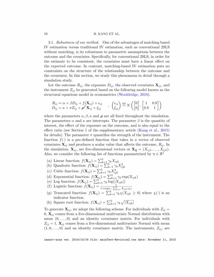
])where the parameters α, β, κ and ρ are all fixed throughout the simulation.The parameters α and κ are intercepts. The parameter β is the quantity ofinterest, the effect of the exposure on the outcome, and is also equal to theeffect ratio (see Section 1 of the supplementary article (Kang et al., 2015)for details). The parameter π quantifies the strength of the instrument. Thefunction f(·) is a pre-defined function that takes in a vector of observedcovariates Xij and produces a scalar value that affects the outcome, Rij . Inthe simulation, Xij , are five-dimensional vectors or Xij = (Xij1, . . . , Xij5).Also, we consider the following list of functions parametrized by γ ∈ R5
(a) Linear function: f(Xij) =∑5
k=1 γkXijk
(b) Quadratic function: f(Xij) =∑5
k=1 γkX2ijk
(c) Cubic function: f(Xij) =∑5
k=1 γkX3ijk
(d) Exponential function: f(Xij) =∑5
k=1 γk exp(Xijk)(e) Log function: f(Xij) =
∑5k=1 γk log(|Xijk|)
(f) Logistic function: f(Xij) = 11+exp(−
∑5k=1Xijkγk)
(g) Truncated function: f(Xij) =∑5
k=1 γkχ(Xijk ≥ 0) where χ(·) is anindicator function.
(h) Square root function: f(Xij) =∑5
k=1 γk√|Xijk|
To generate Xij , we adopt the following scheme. For individuals with Zij =0, Xij comes from a five-dimensional multivariate Normal distribution withmean (0, . . . , 0) and an identity covariance matrix. For individuals withZij = 1, Xij comes from a five-dimensional multivariate Normal with mean(1, 0, . . . , 0) and an identity covariance matrix. The instruments, Zij , are
imsart-aoas ver. 2014/10/16 file: mainText-Revision2.tex date: November 11, 2015
FULL MATCHING IV ESTIMATION 17
Linear
Concentration parameter
Abs
olut
e bi
as
0 10 20 30 40 50
0.0
0.4
0.8
1.2
1.6
Quadratic
Concentration parameterA
bsol
ute
bias
0 10 20 30 40 50
0.0
0.4
0.8
1.2
1.6
Cubic
Concentration parameter
Abs
olut
e bi
as
0 10 20 30 40 50
0.0
0.4
0.8
1.2
1.6
Exponential
Concentration parameter
Abs
olut
e bi
as
0 10 20 30 40 50
0.0
0.4
0.8
1.2
1.6
Log
Concentration parameter
Abs
olut
e bi
as
0 10 20 30 40 50
0.0
0.4
0.8
1.2
1.6
Logistic
Concentration parameter
Abs
olut
e bi
as
0 10 20 30 40 50
0.0
0.4
0.8
1.2
1.6
Truncated
Concentration parameter
Abs
olut
e bi
as
0 10 20 30 40 50
0.0
0.4
0.8
1.2
1.6
Square Root
Concentration parameter
Abs
olut
e bi
as
0 10 20 30 40 50
0.0
0.4
0.8
1.2
1.6
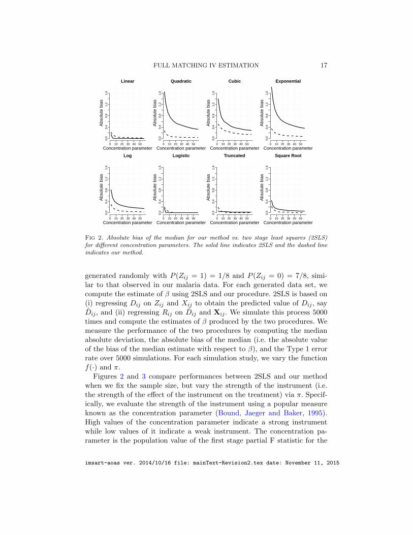
Fig 2. Absolute bias of the median for our method vs. two stage least squares (2SLS)for different concentration parameters. The solid line indicates 2SLS and the dashed lineindicates our method.
generated randomly with P (Zij = 1) = 1/8 and P (Zij = 0) = 7/8, simi-lar to that observed in our malaria data. For each generated data set, wecompute the estimate of β using 2SLS and our procedure. 2SLS is based on(i) regressing Dij on Zij and Xij to obtain the predicted value of Dij , sayDij , and (ii) regressing Rij on Dij and Xij . We simulate this process 5000times and compute the estimates of β produced by the two procedures. Wemeasure the performance of the two procedures by computing the medianabsolute deviation, the absolute bias of the median (i.e. the absolute valueof the bias of the median estimate with respect to β), and the Type 1 errorrate over 5000 simulations. For each simulation study, we vary the functionf(·) and π.
Figures 2 and 3 compare performances between 2SLS and our methodwhen we fix the sample size, but vary the strength of the instrument (i.e.the strength of the effect of the instrument on the treatment) via π. Specif-ically, we evaluate the strength of the instrument using a popular measureknown as the concentration parameter (Bound, Jaeger and Baker, 1995).High values of the concentration parameter indicate a strong instrumentwhile low values of it indicate a weak instrument. The concentration pa-rameter is the population value of the first stage partial F statistic for the
imsart-aoas ver. 2014/10/16 file: mainText-Revision2.tex date: November 11, 2015

18 H. KANG ET AL.
instruments when the treatment is regressed on the instrument and themeasured covariates Xij ; this first stage F statistic is often used to checkinstrument strength where an F below 10 suggests that the instruments areweak (Stock, Wright and Yogo, 2002). The sample size is fixed at 800 where100 individuals have Zij = 1 and 700 individuals have Zij = 0, similar tothe sample size presented in the malaria data. We also vary f(·) based onthe functions listed in the previous paragraph.
Figure 2 measures the absolute bias of the median for 2SLS and ourmethod. When f(·) is a linear function of the observed covariates xij , 2SLSdoes slightly better than our method. 2SLS doing well for the linear functionis to be expected since 2SLS is consistent when the model is linear. However,if f(·) is non-linear, our matching estimator does better than 2SLS andis never substantially worse for all instrument strengths. For example, forquadratic, cubic, exponential, log, and square root functions, our method haslower bias than 2SLS for all strengths of the instrument. For logistic andtruncated functions, our method is similar in performance to 2SLS for allstrengths of the instrument. In the supplementary article (Kang et al., 2015),we also measure the median absolute deviation of 2SLS and our method andwe find that the price we pay for lower bias of our method in a slight increasein dispersion compared to 2SLS.
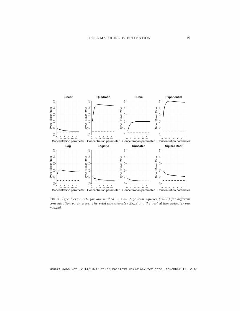
Finally, Figure 3 measures the Type I error rate of 2SLS and our method.Regardless of the function type and the instrument strength, our methodretains the nominal 0.05 rate. In fact, even for the linear case where 2SLS isdesigned to excel, our estimator has the correct Type I error rate for all in-strument strengths while 2SLS has higher Type I error for weak instruments.For all the non-linear functions, the Type I error rate for 2SLS remains abovethe 0.05 line while our estimator maintains the nominal Type I error rate.This provides evidence that our estimator will have the correct 95% coveragefor confidence intervals regardless of non-linearity or instrument strength.
In summary, the simulation study shows promise that our method is gen-erally more robust to assumptions about instrument strength and linearitybetween the outcome and the covariates than 2SLS at the expense of a smallincrease in dispersion.
3.2. Comparison to Frolich (2007). In addition to comparing our methodagainst the most popular IV estimator, 2SLS, we also compare our methodto the non-parametric IV method of Frolich (2007) implemented by Frolichand Melly (2010). The simulation setup is identical to Section 3.1, exceptthat we discretize the exposure value Di so that we can compare our methodto the method in Frolich (2007). Specifically, let D∗ij be defined as Dij in
imsart-aoas ver. 2014/10/16 file: mainText-Revision2.tex date: November 11, 2015
FULL MATCHING IV ESTIMATION 19
Linear
Concentration parameter
Type
I E
rror
Rat
e
0 10 20 30 40 50
0.0
0.1
0.2
0.3
0.4
0.5
Quadratic
Concentration parameter
Type
I E
rror
Rat
e
0 10 20 30 40 50
0.0
0.1
0.2
0.3
0.4
0.5
Cubic
Concentration parameter
Type
I E
rror
Rat
e
0 10 20 30 40 50
0.0
0.1
0.2
0.3
0.4
0.5
Exponential
Concentration parameter
Type
I E
rror
Rat
e
0 10 20 30 40 50
0.0
0.1
0.2
0.3
0.4
0.5
Log
Concentration parameter
Type
I E
rror
Rat
e
0 10 20 30 40 50
0.0
0.1
0.2
0.3
0.4
0.5
Logistic
Concentration parameter
Type
I E
rror
Rat
e
0 10 20 30 40 50
0.0
0.1
0.2
0.3
0.4
0.5
Truncated
Concentration parameter
Type
I E
rror
Rat
e
0 10 20 30 40 50
0.0
0.1
0.2
0.3
0.4
0.5
Square Root
Concentration parameter
Type
I E
rror
Rat
e
0 10 20 30 40 50
0.0
0.1
0.2
0.3
0.4
0.5
Fig 3. Type I error rate for our method vs. two stage least squares (2SLS) for differentconcentration parameters. The solid line indicates 2SLS and the dashed line indicates ourmethod.
imsart-aoas ver. 2014/10/16 file: mainText-Revision2.tex date: November 11, 2015

20 H. KANG ET AL.
Section 3.1, i.e. D∗ij = κ+ πZij + ρTXij + ξij . Then, we define
Dij = χ(D∗ij < −1) + 2χ(−1 ≤ D∗ij < 1) + 3χ(1 ≤ D∗ij)
where χ(·) is the indicator function. The response Rij is generated from thesame model as in Section 3.1, except with a discretetized Dij . The rest ofthe data generating process is identical to Section 3.1.
For each simulated data, we use the code provided by Frolich and Melly(2010) to generate an estimate for β∗, the local average treatment effect,with the default settings for the tuning parameters. We also use our methodto estimate β∗. Finally, for comparison, we run 2SLS on the simulate data.As before, we measure the median absolute deviation and the absolute biasof the median. For each simulation study, we vary the function f(·) and π,the strength of the instrument.
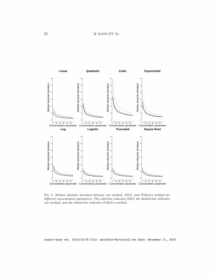
Figures 4 and 5 show the absolute bias and median absolute deviation be-tween the three methods. Generally speaking, both our method and Frolich(2007)’s method do better than 2SLS when f(·) is non-linear. Between ourmethod and Frolich (2007)’s method, in most cases, our method is better orsimilar to the Frolich (2007)’s method when it comes to bias. With regardsto variability, our method and Frolich (2007)’s method are very similar toeach other. For the quadratic, cubic, and exponential functions, our simula-tions show that our method dominates both in bias and variance comparedto Frolich (2007). Further details of the simulation in this Section can befound in the supplementary article (Kang et al., 2015).
4. Data Analysis of the Causal Effect of Malaria on Stunting.
4.1. Background information. Using the new full matching IV methodin this paper, we analyze the data set introduced in Section 1.1 to study thecausal effect of malaria on stunting. Following Kreuels et al. (2009), we onlyconsider children with the heterozygous strand HbAS, the sickle cell trait, orwildtype HbAA and exclude children with the homozygous strand (HbSS),or a different mutation on the same gene leading to hemoglobin C (HbAC,HbCC, HbSC); this reduced the sample size from 1070 to 884. Among 884children, 110 children carried HbAS and 774 children carried HbAA.
The instrument was a binary variable indicating either the HbAS orHbAA genotype. The exposure of interest was the malarial history, whichwas defined as the total number of malarial episodes during the study. Amalaria episode was defined as having a parasite density of more than 500parasites/µl and a body temperature greater than 38C or the mother re-ported a fever within the last 48 hours. The outcome was whether the child
imsart-aoas ver. 2014/10/16 file: mainText-Revision2.tex date: November 11, 2015

FULL MATCHING IV ESTIMATION 21
Linear
Concentration parameter
Abs
olut
e bi
as
0 10 20 30 40 50
0.0
0.5
1.0
1.5
2.0
2.5
3.0
3.5
Quadratic
Concentration parameter
Abs
olut
e bi
as
0 10 20 30 40 50
0.0
0.5
1.0
1.5
2.0
2.5
3.0
3.5
Cubic
Concentration parameter
Abs
olut
e bi
as
0 10 20 30 40 50
0.0
0.5
1.0
1.5
2.0
2.5
3.0
3.5
Exponential
Concentration parameter
Abs
olut
e bi
as
0 10 20 30 40 50
0.0
0.5
1.0
1.5
2.0
2.5
3.0
3.5
Log
Concentration parameter
Abs
olut
e bi
as
0 10 20 30 40 50
0.0
0.5
1.0
1.5
2.0
2.5
3.0
3.5
Logistic
Concentration parameter
Abs
olut
e bi
as
0 10 20 30 40 50
0.0
0.5
1.0
1.5
2.0
2.5
3.0
3.5
Truncated
Concentration parameter
Abs
olut
e bi
as
0 10 20 30 40 50
0.0
0.5
1.0
1.5
2.0
2.5
3.0
3.5
Square Root
Concentration parameter
Abs
olut
e bi
as
0 10 20 30 40 50
0.0
0.5
1.0
1.5
2.0
2.5
3.0
3.5
Fig 4. Absolute bias of the median for our method, 2SLS, and Frolich’s method for differentconcentration parameters. The solid line indicates 2SLS, the dashed line indicates ourmethod, and the dotted line indicates Frolich’s method.
imsart-aoas ver. 2014/10/16 file: mainText-Revision2.tex date: November 11, 2015
22 H. KANG ET AL.
Linear
Concentration parameter
Med
ian
abso
lute
dev
iatio
n
0 10 20 30 40 50
01
23
45
6
Quadratic
Concentration parameter
Med
ian
abso
lute
dev
iatio
n
0 10 20 30 40 50
01
23
45
6
Cubic
Concentration parameter
Med
ian
abso
lute
dev
iatio
n
0 10 20 30 40 50
01
23
45
6
Exponential
Concentration parameter
Med
ian
abso
lute
dev
iatio
n
0 10 20 30 40 50
01
23
45
6
Log
Concentration parameter
Med
ian
abso
lute
dev
iatio
n
0 10 20 30 40 50
01
23
45
6
Logistic
Concentration parameter
Med
ian
abso
lute
dev
iatio
n
0 10 20 30 40 50
01
23
45
6
Truncated
Concentration parameter
Med
ian
abso
lute
dev
iatio
n
0 10 20 30 40 50
01
23
45
6
Square Root
Concentration parameter
Med
ian
abso
lute
dev
iatio
n
0 10 20 30 40 50
01
23
45
6
Fig 5. Median absolute deviation between our method, 2SLS, and Frolich’s method fordifferent concentration parameters. The solid line indicates 2SLS, the dashed line indicatesour method, and the dotted line indicates Frolich’s method.
imsart-aoas ver. 2014/10/16 file: mainText-Revision2.tex date: November 11, 2015

FULL MATCHING IV ESTIMATION 23
was stunted at the last recorded visit, which occurred when the child wasapproximately two years old. The difference in episodes of malaria betweenchildren with HbAS and HbAA is significant (Risk ratio: 0.82, p-value: 0.02,95% CI: (0.70, 0.97)), indicating that the sickle cell trait instrument satisfiesAssumption (A1) of being associated with the exposure.
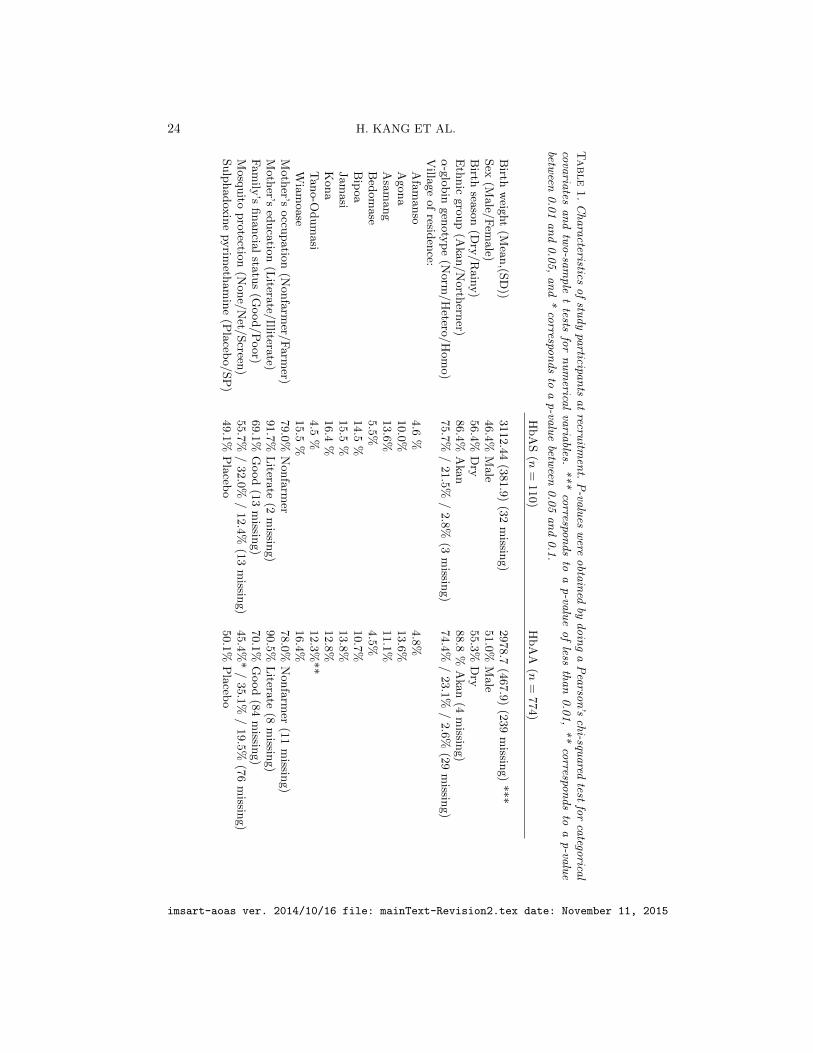
Table 1 summarizes all the measured covariates in this data. All the co-variates were collected at the beginning of the study, which is three monthsafter the child’s birth. We will match on all these covariates for reasons thatwill be explained below. Broadly speaking, for valid inference of the causaleffect using instrumental variables, we would like to include all confoundersfor the instrument-outcome relationship, i.e. covariates that are determinedbefore (or at the same time and not affected by) the sickle cell trait and thatare associated with the outcome. The following covariates in Table 1, villageof residence, sex, ethnicity, birth season, and alpha-globin genotype, repre-sent such potential confounders. They occur before (or at the same time andare not affected by) the sickle cell trait and they could be associated withthe outcome of stunting through population stratification. If these covariateswere the only instrument-outcome confounders, then we would not need toconsider matching for other covariates.
However, other possible confounders in our data include family’s socioeco-nomic status and parents’ sickle cell genotype. Family’s socioeconomic statusmay be associated with the sickle cell trait through population stratificationand can affect the outcome of stunting through the nutrition and hygienicenvironment of the child. Parents’ sickle cell genotype is associated with thechild’s sickle cell genotype because of the properties of genetic inheritanceand may be associated with the outcome of stunting through populationstratification. Although these two possible confounders were not measuredat the time of instrument assignment (i.e. the child’s conception), the fol-lowing covariates in Table 1, birthweight, mother’s occupation, mother’seducation, family’s financial status, and mosquito protection are proxies forthese variables. Specifically, mother’s occupation, mother’s education, andfamily’s financial status measured three months after the child’s birth areproxies of family’s socioeconomic status at the time of the child’s concep-tion. Mosquito protection and birthweight are proxies for parents’ sicklecell genotype. In particular, mosquito protection at the time of the child’sconception (i.e. whether the family’s home is protected by nets, screens,or nothing) may be associated with parents’ sickle cell genotype because afamily might be less likely to seek additional mosquito protection if mem-bers of the family are naturally protected by being carriers of the sicklecell genotype; one can see in Table 1 that children carrying HbAS tend to
imsart-aoas ver. 2014/10/16 file: mainText-Revision2.tex date: November 11, 2015
24 H. KANG ET AL.
Table
1.
Ch
ara
cteristicso
fstu
dy
participa
nts
at
recruitm
ent.
P-va
lues
were
obta
ined
byd
oin
ga
Pea
rson’s
chi-squ
ared
testfo
rca
tegorica
lco
varia
tesa
nd
two
-sam
ple
ttests
for
nu
merica
lva
riables.
**
*co
rrespon
ds
toa
p-va
lue
of
lessth
an
0.0
1,
**
correspo
nd
sto
ap
-valu
ebetw
een0
.01
an
d0
.05
,a
nd
*co
rrespon
ds
toa
p-va
lue
between
0.0
5a
nd
0.1
.
HbA
S(n
=110)
HbA
A(n
=774)
Birth
weig
ht
(Mea
n,(S
D))
3112.4
4(3
81.9
)(3
2m
issing)
2978.7
(467.9
)(2
39
missin
g)
***
Sex
(Male/
Fem
ale)
46.4
%M
ale
51.0
%M
ale
Birth
seaso
n(D
ry/R
ain
y)
56.4
%D
ry55.3
%D
ryE
thnic
gro
up
(Aka
n/N
orth
erner)
86.4
%A
kan
88.8
%A
kan
(4m
issing)
α-g
lobin
gen
oty
pe
(Norm
/H
etero/H
om
o)
75.7
%/
21.5
%/
2.8
%(3
missin
g)
74.4
%/
23.1
%/
2.6
%(2
9m
issing)
Villa
ge
of
residen
ce:A
fam
anso
4.6
%4.8
%A
gona
10.0
%13.6
%A
sam
ang
13.6
%11.1
%B
edom
ase
5.5
%4.5
%B
ipoa
14.5
%10.7
%Jam
asi
15.5
%13.8
%K
ona
16.4
%12.8
%T
ano-O
dum
asi
4.5
%12.3
%**
Wia
moase
15.5
%16.4
%M
oth
er’soccu
patio
n(N
onfa
rmer/
Farm
er)79.0
%N
onfa
rmer
78.0
%N
onfa
rmer
(11
missin
g)
Moth
er’sed
uca
tion
(Litera
te/Illitera
te)91.7
%L
iterate
(2m
issing)
90.5
%L
iterate
(8m
issing)
Fam
ily’s
financia
lsta
tus
(Good/P
oor)
69.1
%G
ood
(13
missin
g)
70.1
%G
ood
(84
missin
g)
Mosq
uito
pro
tection
(None/
Net/
Screen
)55.7
%/
32.0
%/
12.4
%(1
3m
issing)
45.4
%*
/35.1
%/
19.5
%(7
6m
issing)
Sulp
hadox
ine
pyrim
etham
ine
(Pla
cebo/SP
)49.1
%P
laceb
o50.1
%P
laceb
o
imsart-aoas ver. 2014/10/16 file: mainText-Revision2.tex date: November 11, 2015
FULL MATCHING IV ESTIMATION 25
have less mosquito protection than child carrying HbAA. Birthweight maybe associated with maternal sickle cell genotype because a mother havingHbAS may be protected from malaria during pregnancy, which may increasebirthweight (Eisele et al., 2012).
But, matching on covariates that are measured or determined after theinstrument such as birthweight, mosquito protection, and family’s socioe-conomic status three months after the child’s birth could create bias if theinstrument could alter these values (Rosenbaum, 1984). However, we thinkthe child’s sickle cell trait instrument does not alter these covariates becausechildren are generally protected from malaria in the first three months of lifedue to maternal antibodies (Snow et al., 1998) and parents were generallynot aware of the child’s sickle cell genotype. Consequently, the child’s sicklecell genotype does not affect the child’s birthweight, family decisions aboutmosquito protection, and family’s socioeconomic status at the time the childis three months old and these variables are effectively pre-instrument covari-ates so that matching for them does not create bias (Rosenbaum, 1984; Hol-land, 1986). In short, we match for all the covariates in Table 1 because theyare either pre-instrument potential confounders or effectively pre-instrumentproxies for unmeasured potential confounders.
Finally, we note that some of the covariates in Table 1 may not be highlyassociated with the sickle cell trait genotype. For example, sulpadoxinepyrimethamine vs. placebo was randomly assigned as part of a randomizedtrial. However, we still have chosen to match on all the covariates becauseeach covariate may be associated with the outcome and matching a covariatethat is associated with the outcome increases efficiency and reduces sensi-tivity to unobserved biases (Rosenbaum, 2005; Zubizarreta, Paredes andRosenbaum, 2014). Furthermore, Rubin (2009) argues for erring on the sideof being inclusive when deciding which variables to match on (i.e. controlfor) in an observational study. Failure to match for a covariate that hasan important effect on outcome and is slightly out of balance can causesubstantial bias.
In terms of the balance of the covariates in Table 1, before matching,we see that there are a few significant differences between the HbAS andHbAA groups, most notably in birth weight, village of birth, and mosquitoprotection status. Children with the sickle cell trait (HbAS) tend to havehigh birth weights and lack any protection against mosquitos compared toHbAA children. Also, children living in the village of Tano-Odumasi tend toinherit HbAA more frequently than HbAS. Any one of these differences cancontribute to the violation of IV assumption (A3) in Section 2.3 if we do notcontrol for these differences. For instance, it is possible that children with
imsart-aoas ver. 2014/10/16 file: mainText-Revision2.tex date: November 11, 2015
26 H. KANG ET AL.
low birth weights were malnourished at birth, making them more prone tomalarial episodes and stunted growth compared to children with high birthweights. We must control for these differences to eliminate this possibility,which we do through full matching.
4.2. Implementation of full matching on data. We conduct full matchingon all observed covariates. In particular, we group children with HbAS andwithout HbAS based on all the observed characteristics in Table 1 as wellas match for patterns of missingness. To measure similarity of the observedand missing covariates, we use the rank-based Mahalanobis distance as thedistance metric for covariate similarity (Rosenbaum, 2010). In addition, wecompute propensity scores by logistic regression. Here, the propensity scoreis an instrumental propensity score, which is the probability of having thesickle cell trait given the measured confounders (Cheng, 2011). In addi-tion, children with missing values in their covariates were matched to otherchildren with similar patterns of missing data (Rosenbaum, 2010). Oncecovariate similarity was calculated, the matching algorithm optmatch in R(Hansen and Klopfer, 2006) matched children carrying HbAS with childrencarrying HbAA in a way that within each matched set, their covariates aresimilar.
Figure 6 shows covariate balance before and after full matching usingabsolute standardized differences. Absolute standardized differences beforematching are computed by taking the difference of the means between chil-dren with HbAS and HbAA for each covariate, taking the absolute value ofit, and normalizing it by the within group standard deviation before match-ing (the square root of the average of the variances within the groups).Absolute standardized differences after matching are computed by takingthe differences of the means between children with HbAS and HbAA withineach strata, averaging this difference across strata, taking the absolute valueof it, and normalizing it by the same within group standard deviation beforematching as before. Before matching, there are differences in birth weight,mosquito protection, and village of residence between children with HbASand HbAA. After matching, these covariates are balanced. Specifically, thestandardized differences for birth weight, village of residence, and mosquitoprotection, are under 0.1 indicating balance (Normand et al., 2001). In fact,all the covariates are balanced after matching and the p-values used to testthe differences between HbAS and HbAA in Table 1 are no longer signifi-cant after matching. Hansen (2004) discusses how the size of matched setsin full matching can be restricted. In the supplementary article (Kang et al.,2015), we compare different restrictions on full matching versus unrestricted
imsart-aoas ver. 2014/10/16 file: mainText-Revision2.tex date: November 11, 2015

FULL MATCHING IV ESTIMATION 27
Absolute standardized differences of covariates
Absolute standardized differences
Mosquito protection missing
Mother’s financial status missing
Mother’s education missing
Mother’s occupation missing
Alpha−globin genotype missing
Ethnicity missing
Birth weight missing
Missing Covariates:
Sulphadoxine pyrimethamine
Other:
Mosquito protection (Nets)
Mosquito protection (Screen)
Mother’s financial status
Mother’s education
Mother’s occupation
Mother and Household:
Wiamoase
Tano−Odumasi
Kona
Jamasi
Bipoa
Bedomase
Asamang
Agona
Village of Residence:
Alpha−globin genotype (Homo)
Alpha−globin genotype (Hetero)
Ethnicity
Birth season
Gender
Birth weight
Birth:
0.00 0.05 0.10 0.15 0.20
Fig 6. Absolute standardized differences before and after full matching. Unfilled circlesindicate differences before matching and filled circles indicate differences after matching.
imsart-aoas ver. 2014/10/16 file: mainText-Revision2.tex date: November 11, 2015

28 H. KANG ET AL.
Table 2Estimates of the causal effect using full matching compared to two-stage least squares and
multiple regression.
Methods Estimate P-value 95% confidence interval
Our method 0.22 0.011 (0.044, 1)Two stage least squares 0.21 0.14 (-0.065, 0.47)Multiple regression 0.018 0.016 (0.0034, 0.033)
full matching in terms of balance and efficiency. In short, the analysis revealsthat unrestricted full matching creates the most covariate balance by a sub-stantial amount while having a only slight decrease in efficiency comparedto other full matching schemes considered and hence, we use unrestrictedfull matching.
4.3. Estimate of causal effect of malaria on stunting. Table 2 shows theestimates of the causal effect of malaria on stunting from different methods,specifically our matching-based method, conventional two stage least squares(2SLS), and multiple regression. Our matching-based method computed theestimate by the procedure outlined in Section 2.5. 2SLS computed the es-timate by regressing all the measured covariates and the instrument on theexposure and using the prediction from that regression and the measuredcovariates to obtain the estimated effect. Inference for 2SLS was derived us-ing standard asymptotic Normality arguments (Wooldridge, 2010). Finally,the multiple regression estimate was derived by regressing the outcome onthe exposure and the covariates and the inference on the estimate was basedon a standard t test.
We see that the full matching method estimates λ to be 0.22. That is,the risk of stunting among children with the sickle cell trait is estimated todecrease by 0.22 times the average malaria episodes prevented by the sicklecell trait. Furthermore, we reject the hypothesis H0 : λ = 0, that malariadoes not cause stunting, at the 0.05 significance level. The confidence intervalλ is (0.044, 1.0). Even the lower limit of this confidence interval of 0.044means that malaria has a substantial effect on stunting; it would mean thatthe risk of stunting among children with the sickle cell trait is decreased by0.044 times the average malaria episodes prevented by the sickle cell trait.
The estimate based on 2SLS is 0.21, similar to our method. However, ourmethod achieves statistical significance but 2SLS does not. Also, multipleregression, which does not control for unmeasured confounders, estimates amuch smaller effect of 0.018.
Table 3 shows the sensitivity analysis due to unmeasured confounders.Specifically, we measure how sensitive our estimate and the p-value in Table
imsart-aoas ver. 2014/10/16 file: mainText-Revision2.tex date: November 11, 2015

FULL MATCHING IV ESTIMATION 29
Table 3Sensitivity analysis for instrumental variables with full matching. The range of
significance is the range of p-values over the different possible distributions of theunmeasured confounder given a particular value of Γ, which represents the effect of
unobserved confounders on the inference of λ.
Gamma Range of significance
1.1 (0.0082, 0.041)1.2 (0.0034, 0.074)1.3 (0.0015, 0.12)
2 is to violation of assumption (A3) in Section 2.3, even after matching. Wesee that our results are somewhat sensitive to unmeasured confounders atthe 0.05 significance level. If there is an unmeasured confounder that in-creases the odds of inheriting HbAS over HbAA by 10%, i.e. Γ = 1.1, thenwe would still have strong evidence that malaria causes stunting. But, if anunmeasured confounder increases the odds of inheriting HbAS over HbAAin a child by 20% (i.e. Γ = 1.2), the range of possible p-values includes 0.05,the significance level, meaning that we would not reject the null hypothesisof H0 : λ = 0, that malaria does not cause stunting. In the supplemen-tary article (Kang et al., 2015), we amplify the sensitivity analysis followingRosenbaum and Silber (2009).
5. Summary. Overall, in contrast to regression-based IV estimationprocedures like 2SLS, our full matching IV method (i) provided a clear wayto assess the balance of observed covariates and design the study withoutlooking at the outcome data and (ii) provided a method to quantify the effectof unmeasured confounders on our inference of the causal effect. Our methodmade it explicitly clear how these covariates were adjusted by stratifying in-dividuals based on similar covariate values. Finally, like in a randomizedexperiment, our analysis only looked at the outcome data once the balancewas acceptable, i.e. once the differences in birth weight, village of residence,and mosquito protection between children with HbAS and HbAA were con-trolled for. If the balance was unacceptable, then comparing the outcomesbetween the two groups would not provide reliable causal inference sinceany differences in the outcome can be attributed to the differences in thecovariates. In contrast, conventional 2SLS can only analyze the causal rela-tionship in the presence of outcome data, making the outcome data necessarythroughout the entire analysis. Finally, our method is robust to parametricmodeling assumptions between the outcome and the covariates with respectto Type I error and point estimate, which cannot be said about 2SLS.
At the expense of these benefits, especially blinding and transparencywith regards to covariate balance, unfortunately matching estimators tend
imsart-aoas ver. 2014/10/16 file: mainText-Revision2.tex date: November 11, 2015
30 H. KANG ET AL.
to be less efficient than 2SLS or some of the semiparametric methods men-tioned in Section 1.3 when the semiparametric methods’ assumptions hold.In practice, our estimator’s blinding and transparency can be a powerfuldesign and visual tool for applied researchers to assess the validity of thecausal conclusions. However, a more careful exploration of the trade-offsbetween the efficiency of our estimator and the efficiency of some of thesemiparametric and non-parametric methods is an interesting direction forfuture research.
References.
Abadie, A. (2003). Semiparametric instrumental variable estimation of treatment re-sponse models. Journal of Econometrics 113 231 - 263.
Aidoo, M., Terlouw, D. J., Kolczak, M. S., McElroy, P. D., ter Kuile, F. O.,Kariuki, S., Nahlen, B. L., Lal, A. A. and Udhayakumar, V. (2002). Protectiveeffects of the sickle cell gene against malaria morbidity and mortality. The Lancet 3591311-1312.
Angrist, J. D. and Imbens, G. W. (1995). Two-Stage Least Squares Estimation ofAverage Causal Effects in Models with Variable Treatment Intensity. Journal of theAmerican Statistical Association 90 431-442.
Angrist, J. D., Imbens, G. W. and Rubin, D. B. (1996). Identification of Causal EffectsUsing Instrumental Variables. Journal of the American Statistical Association 91 444–455.
Angrist, J. D. and Krueger, A. B. (1991). Does Compulsory School Attendance AffectSchooling and Earnings? The Quarterly Journal of Economics 106 979–1014.
Ashcroft, M. T., Desai, P. and Richardson, S. A. (1976). Growth, behaviour, andeducational achievement of Jamaican children with sickle-cell trait. British MedicalJournal 1 1371-1373.
Ashcroft, M. T., Desai, P., Grell, G. A., Serjeant, B. E. and Serjeant, G. R.(1978). Heights and weights of West Indian children with the sickle cell trait. Archivesof Disease in Childhood 53 596-598.
Baiocchi, M., Cheng, J. and Small, D. S. (2014). Instrumental variable methods forcausal inference. Statistics in Medicine 33 2297–2340.
Baiocchi, M., Small, D. S., Lorch, S. and Rosenbaum, P. R. (2010). Building astronger instrument in an observational study of perinatal care for premature infants.Journal of the American Statistical Association 105 1285-1296.
Bound, J., Jaeger, D. A. and Baker, R. M. (1995). Problems with instrumental vari-ables estimation when the correlation between instruments and the endogenous variableis weak. Journal of the American Statistical Association 90 443–450.
Brookhart, M. A. and Schneeweiss, S. (2007). Preference-based instrumental variablemethods for the estimation of treatment effects: assessing validity and interpretingresults. The International Journal of Biostatistics 3 14.
Card, D. (1995). Using geographic variations in college proximity to estimate the returnto schooling. University of Toronto Press.
Cheng, J. (2011). Using the instrumental propensity score in observational studies forcausal effects. Joint Statistical Meeting Presentation.
Cheng, J., Qin, J. and Zhang, B. (2009). Semiparametric estimation and inference fordistributional and general treatment effects. Journal of the Royal Statistical Society:Series B (Statistical Methodology) 71 881–904.
imsart-aoas ver. 2014/10/16 file: mainText-Revision2.tex date: November 11, 2015

FULL MATCHING IV ESTIMATION 31
Cholera, R., Brittain, N. J., Gillrie, M. R., Lopera-Mesa, T. M., Diakit, S. A. S.,Arie, T., Krause, M. A., Guindo, A., Tubman, A., Fujioka, H., Diallo, D. A.,Doumbo, O. K., Ho, M., Wellems, T. E. and Fairhurst, R. M. (2008). Im-paired cytoadherence of Plasmodium falciparum-infected erythrocytes containing sicklehemoglobin. Proceedings of the National Academy of Sciences 105 991-996.
Cochran, W. G. (1965). The planning of observational studies of human populations.Journal of the Royal Statistical Society: Series A (General) 234-266.
Crookston, B. T., Alder, S. C., Boakye, I., Merrill, R. M., Amuasi, J. H.,Porucznik, C. A., Stanford, J. B., Dickerson, T. T., Dearden, K. A.,Hale, D. C., Sylverken, J., Snow, B. S., Osei-Akoto, A. and Ansong, D. (2010).Exploring the relationship between chronic undernutrition and asymptomatic malariain Ghanaian children. Malaria Journal 9.
Davey Smith, G. and Ebrahim, S. (2003). Mendelian randomization: can genetic epi-demiology contribute to understanding environmental determinants of disease? Inter-national Journal of Epidemiology 32 1-22.
Deen, J. L., Walraven, G. E. L. and von Seidlein, L. (2002). Increased Risk forMalaria in Chronically Malnourished Children Under 5 Years of Age in Rural Gambia.Journal of Tropical Pediatrics 48 78-83.
Deribew, A., Alemseged, F., Tessema, F., Sena, L., Birhanu, Z., Zeynudin, A.,Sudhakar, M., Abdo, N., Deribe, K. and Biadgilign, S. (2010). Malaria and Under-Nutrition: A Community Based Study Among Under-Five Children at Risk of Malaria,South-West Ethiopia. PLoS One 5 e10775.
Ehrhardt, S., Burchard, G. D., Mantel, C., Cramer, J. P., Kaiser, S., Kubo, M.,Otchwemah, R. N., Bienzle, U. and Mockenhaupt, F. P. (2006). Malaria, Ane-mia, and Malnutrition in African ChildrenDefining Intervention Priorities. Journal ofInfectious Diseases 194 108-114.
Eisele, T. P., Larsen, D. A., Anglewicz, P. A., Keating, J., Yukich, J., Ben-nett, A., Hutchinson, P. and Steketee, R. W. (2012). Malaria prevention inpregnancy, birthweight, and neonatal mortality: a meta-analysis of 32 national cross-sectional datasets in Africa. The Lancet Infectious Diseases 12 942-949.
Fillol, F., Sarr, J. B., Boulanger, D., Cisse, B., Sokhna, C., Riveau, G., Si-mondon, K. B. and Remoue, F. (2009). Impact of child malnutrition on the specificanti-Plasmodium falciparum antibody response. Malaria Journal 8 116.
Friedman, M. J. (1978). Erythrocytic mechanism of sickle cell resistance to malaria.Proceedings of the National Academy of Sciences 75 1994-1997.
Friedman, M. J. and Trager, W. (1981). The biochemistry of resistance to malaria.Scientific American 244 154-155.
Frolich, M. (2007). Nonparametric IV estimation of local average treatment effects withcovariates. Journal of Econometrics 139 35-75.
Frolich, M. and Melly, B. (2010). Estimation of quantile treatment effects with Stata.Stata Journal 10 423-457.
Genton, B., Al-Yaman, F., Ginny, M., Taraika, J. and Alpers, M. P. (1998). Re-lation of anthropometry to malaria morbidity and immunity in Papua New Guineanchildren. The American Journal of Clinical Nutrition 68 734-41.
WHO Multicentre Growth Reference Study Group (2006). WHO Child GrowthStandards based on length/height, weight and age. Acta Paediatrica. Supplement 45076–85.
Hansen, B. B. (2004). Full Matching in an Observational Study of Coaching for the SAT.Journal of the American Statistical Association 99 609–618.
Hansen, B. B. and Klopfer, S. O. (2006). Optimal Full Matching and Related Designs
imsart-aoas ver. 2014/10/16 file: mainText-Revision2.tex date: November 11, 2015

32 H. KANG ET AL.
via Network Flows. Journal of Computational and Graphical Statistics 15 609-627.Haviland, A., Nagin, D. S. and Rosenbaum, P. R. (2007). Combining Propensity Score
Matching and Group-Based Trajectory Analysis in an Observational Study. Psycholog-ical Methods 12 247.
Hernan, M. A. and Robins, J. M. (2006). Instruments for Causal Inference: An Epi-demiologist’s Dream? Epidemiology 17 360–372.
Hodges, J. L. and Lehmann, E. L. (1963). Estimation of location based on ranks. Annalsof Mathematical Statistics 34 598-611.
Holland, P. W. (1986). Statistics and Causal Inference: Rejoinder. Journal of the Amer-ican Statistical Association 81 968-970.
Holland, P. W. (1988). Causal Inference, Path Analysis, and Recursive Structural Equa-tions Models. Sociological Methodology 18 449-484.
Imbens, G. W. and Rubin, D. B. (1997). Bayesian Inference for Causal Effects in Ran-domized Experiments with Noncompliance. The Annals of Statistics 25 305–327.
Kang, H., Kreuels, B., Adjei, O., Krumkamp, R., May, J. and Small, D. S. (2013).The causal effect of malaria on stunting: a Mendelian randomization and matchingapproach. International Journal of Epidemiology 42 1390-1398.
Kang, H., Kreuels, B., May, J. and Small, D. S. (2015). Supplement to “Full matchingapproach to instrumental variables estimation with application to the effect of malariaon stunting”.
Keele, L. J. and Morgan, J. (2013). Stronger Instruments by Design. Working Paper.Kobbe, R., Kreuzberg, C., Adjei, S., Thompson, B., Langefeld, I., Thomp-
son, P. A., Abruquah, H. H., Kreuels, B., Ayim, M., Busch, W., Marks, F.,Amoah, K., Opoku, E., Meyer, C. G., Adjei, O. and May, J. (2007). A Random-ized Controlled Trial of Extended Intermittent Preventive Antimalarial Treatment inInfants. Clinical Infectious Diseases 45 16-25.
Kramer, M. S., Rooks, Y. and Pearson, H. A. (1978). Growth and developmentin children with sickle-cell trait: a prospective study of matched pairs. New EnglandJournal of Medicine 299 686-689.
Kreuels, B., Ehrhardt, S., Kreuzberg, C., Adjei, S., Kobbe, R., Burchard, G.,Ehmen, C., Ayim, M., Adjei, O. and May, J. (2009). Sickle cell trait (HbAS) andstunting in children below two years of age in an area of high malaria transmission.Malaria Journal 8 16.
Kreuels, B., Kreuzberg, C., Kobbe, R., Ayim-Akonor, M., Apiah-Thompson, P.,Thompson, B., Ehmen, C., Adjei, S., Langefeld, I., Adjei, O. and May, J. (2010).Differing effects of HbS and HbC traits on uncomplicated falciparum malaria, anemia,and child growth. Blood 115 4551–4558.
May, J., Evans, J. A., Timmann, C., Ehmen, C., Busch, W., Thye, T., Ag-benyega, T. and Horstmann, R. D. (2007). Hemoglobin Variants and Disease Man-ifestations in Severe Falciparum Malaria. Journal of the American Medical Association297 2220–2226.
Normand, S.-L. T., Landrum, M. B., Guadagnoli, E., Ayanian, J. Z., Ryan, T. J.,Cleary, P. D. and McNeil, B. J. (2001). Validating recommendations for coronaryangiography following acute myocardial infarction in the elderly: a matched analysisusing propensity scores. Journal of Clinical Epidemiology 54 387–398.
Nyakeriga, A. M., Troye-Blomberg, M., Chemtai, A. K., Marsh, K. andWilliams, T. N. (2004). Malaria and Nutritional Status in Children Living on theCoast of Kenya. Scandinavian Journal of Immunology 59 615–616.
Ogburn, E. L., Rotnitzky, A. and Robins, J. M. (2015). Doubly robust estimation ofthe local average treatment effect curve. Journal of the Royal Statistical Society: Series
imsart-aoas ver. 2014/10/16 file: mainText-Revision2.tex date: November 11, 2015
FULL MATCHING IV ESTIMATION 33
B (Statistical Methodology) 77 373–396.World Health Organization (2014). World Malaria Report 2014. World Health Orga-
nization.Rehan, N. (1981). Growth status of children with and without sickle cell trait. Clinical
Pediatrics 20 705–709.Rosenbaum, P. R. (1984). The Consequences of Adjustment for a Concomitant Variable
That Has Been Affected by the Treatment. Journal of the Royal Statistical Society.Series A 147 656–666.
Rosenbaum, P. R. (1991). A Characterization of Optimal Designs for ObservationalStudies. Journal of the Royal Statistical Society. Series B. Methodological 53 597-610.
Rosenbaum, P. R. (2002). Observational Studies, second ed. Springer Series in Statistics.Springer-Verlag, New York.
Rosenbaum, P. R. (2005). Heterogeneity and Causality: Unit Heterogeneity and DesignSensitivity in Observational Studies. American Statistician 59 147-152.
Rosenbaum, P. R. (2010). Design of Observational Studies. Springer Series in Statistics.Springer, New York.
Rosenbaum, P. R. and Silber, J. H. (2009). Amplification of Sensitivity Analysis inMatched Observational Studies. Journal of the American Statistical Association 1041398-1405.
Rubin, D. B. (1980). Comment on “Randomized Analysis of Experimental Data: TheFisher Randomization Test”. Journal of the American Statistical Association 75 591-593.
Rubin, D. B. (2007). The design versus the analysis of observational studies for causaleffects: parallels with the design of randomized trials. Statistics in Medicine 26 20-36.
Rubin, D. B. (2009). Should observational studies be designed to allow lack of balance incovariate distributions across treatment groups? Statistics in Medicine 28 1420-1423.
Rubin, D. B. and Waterman, R. P. (2006). Estimating the causal effects of marketinginterventions using propensity score methodology. Statistical Science 206-222.
Snow, R. W., Nahlen, B., Palmer, A., Donnelly, C. A., Gupta, S. and Marsh, K.(1998). Risk of severe malaria among African infants: direct evidence of clinical protec-tion during early infancy. Journal of Infectious Diseases 177 819-822.
Stock, J. H., Wright, J. H. and Yogo, M. (2002). A Survey of Weak Instrumentsand Weak Identification in Generalized Method of Moments. Journal of Business &Economic Statistics 20.
Stuart, E. A. (2010). Matching methods for causal inference: A review and a look for-ward. Statistical Science 25 1.
Swanson, S. A. and Hernan, M. A. (2013). Commentary: How to Report InstrumentalVariable Analyses (Suggestions Welcome). Epidemiology 24 370–374.
Tan, Z. (2006). Regression and Weighting Methods for Causal Inference Using Instru-mental Variables. Journal of the American Statistical Association 101 1607-1618.
Taylor, S. M., Parobek, C. M. and Fairhurst, R. M. (2012). Haemoglobinopathiesand the clinical epidemiology of malaria: a systematic review and meta-analysis. TheLancet Infectious Diseases 12 457-468.
Williams, T. N., Mwangi, T. W., Roberts, D. J., Alexander, N. D., Weather-all, D. J., Wambua, S., Kortok, M., Snow, R. W. and Marsh, K. (2005). AnImmune Basis for Malaria Protection by the Sickle Cell Trait. PLoS medicine 2 e128.
Wooldridge, J. M. (2010). Econometric Analysis of Cross Section and Panel Data, 2nded. ed. MIT press.
Yang, F., Zubizarreta, J. R., Small, D. S., Lorch, S. and Rosenbaum, P. R. (2014).Dissonant Conclusions When Testing the Validity of an Instrumental Variable. The
imsart-aoas ver. 2014/10/16 file: mainText-Revision2.tex date: November 11, 2015

34 H. KANG ET AL.
American Statistician 68 253-263.Zubizarreta, J. R., Paredes, R. D. and Rosenbaum, P. R. (2014). Matching for
Balance, Pairing for Heterogeneity in an Observational Study of the Effectiveness ofFor-profit and Not-for-profit High Schools in Chile. Annals of Applied Statistics 1 204-231.
Zubizarreta, J. R., Small, D. S., Goyal, N. K., Lorch, S. and Rosenbaum, P. R.(2013). Stronger instruments via integer programming in an observational study of latepreterm birth outcomes. The Annals of Applied Statistics 7 25–50.
APPENDIX A: SUPPLEMENTARY MATERIALS: REVIEW OFNOTATION
We adopt the notation in Section 2.1 of the main manuscript. Also, wedefine the effect ratio, λ, our estimator T (λ0), and S2(λ0) identically asSections 2.4 and 2.5 of the main text.
λ =
∑Ii=1
∑nij=1 r
(d1ij)1ij − r(d0ij)
0ij∑Ii=1
∑nij=1 d1ij − d0ij
(9)
T (λ0) =1
I
I∑i=1
Vi(λ0)(10)
S2(λ0) =1
I(I − 1)
I∑i=1
Vi(λ0)− T (λ0)2(11)
where
Vi(λ0) =nimi
ni∑j=1
Zij(Rij − λ0Dij)−ni
ni −mi
ni∑j=1
(1− Zij)(Rij − λ0Dij)
APPENDIX B: SUPPLEMENTARY MATERIALS: IDENTIFICATIONAND INTERPRETATION OF THE EFFECT RATIO
Let χ(·) be an indicator function. Under the IV assumptions laid outin Section 2.3 of the main paper and the monotonicity assumption whered1ij ≥ d0ij , we can identify the effect ratio and interpret it as the weightedaverage of the unit causal effect of the exposure on the treatment among in-dividuals whose exposure was affected by the instrument. This is formalizedin Proposition 1.
Proposition 1. Suppose the IV assumptions, (A1)-(A3), and SUTVAin Section 2.3 of the main manuscript holds and the exposure ranges from
imsart-aoas ver. 2014/10/16 file: mainText-Revision2.tex date: November 11, 2015
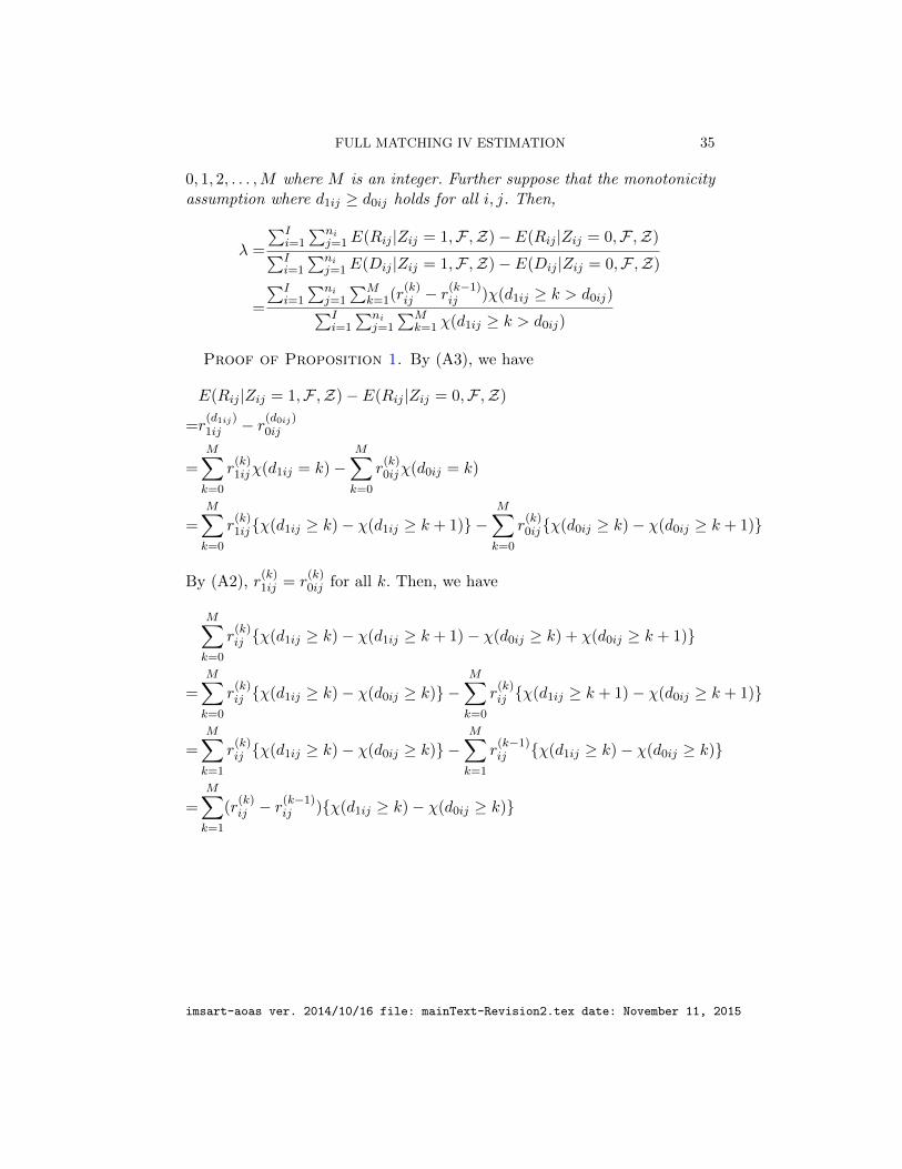
FULL MATCHING IV ESTIMATION 35
0, 1, 2, . . . ,M where M is an integer. Further suppose that the monotonicityassumption where d1ij ≥ d0ij holds for all i, j. Then,
λ =
∑Ii=1
∑nij=1E(Rij |Zij = 1,F ,Z)− E(Rij |Zij = 0,F ,Z)∑I
i=1
∑nij=1E(Dij |Zij = 1,F ,Z)− E(Dij |Zij = 0,F ,Z)
=
∑Ii=1
∑nij=1
∑Mk=1(r
(k)ij − r
(k−1)ij )χ(d1ij ≥ k > d0ij)∑I
i=1
∑nij=1
∑Mk=1 χ(d1ij ≥ k > d0ij)
Proof of Proposition 1. By (A3), we have
E(Rij |Zij = 1,F ,Z)− E(Rij |Zij = 0,F ,Z)
=r(d1ij)1ij − r(d0ij)
0ij
=M∑k=0
r(k)1ijχ(d1ij = k)−
M∑k=0
r(k)0ijχ(d0ij = k)
=
M∑k=0
r(k)1ijχ(d1ij ≥ k)− χ(d1ij ≥ k + 1) −
M∑k=0
r(k)0ijχ(d0ij ≥ k)− χ(d0ij ≥ k + 1)
By (A2), r(k)1ij = r
(k)0ij for all k. Then, we have
M∑k=0
r(k)ij χ(d1ij ≥ k)− χ(d1ij ≥ k + 1)− χ(d0ij ≥ k) + χ(d0ij ≥ k + 1)
=M∑k=0
r(k)ij χ(d1ij ≥ k)− χ(d0ij ≥ k) −
M∑k=0
r(k)ij χ(d1ij ≥ k + 1)− χ(d0ij ≥ k + 1)
=
M∑k=1
r(k)ij χ(d1ij ≥ k)− χ(d0ij ≥ k) −
M∑k=1
r(k−1)ij χ(d1ij ≥ k)− χ(d0ij ≥ k)
=M∑k=1
(r(k)ij − r
(k−1)ij )χ(d1ij ≥ k)− χ(d0ij ≥ k)
imsart-aoas ver. 2014/10/16 file: mainText-Revision2.tex date: November 11, 2015
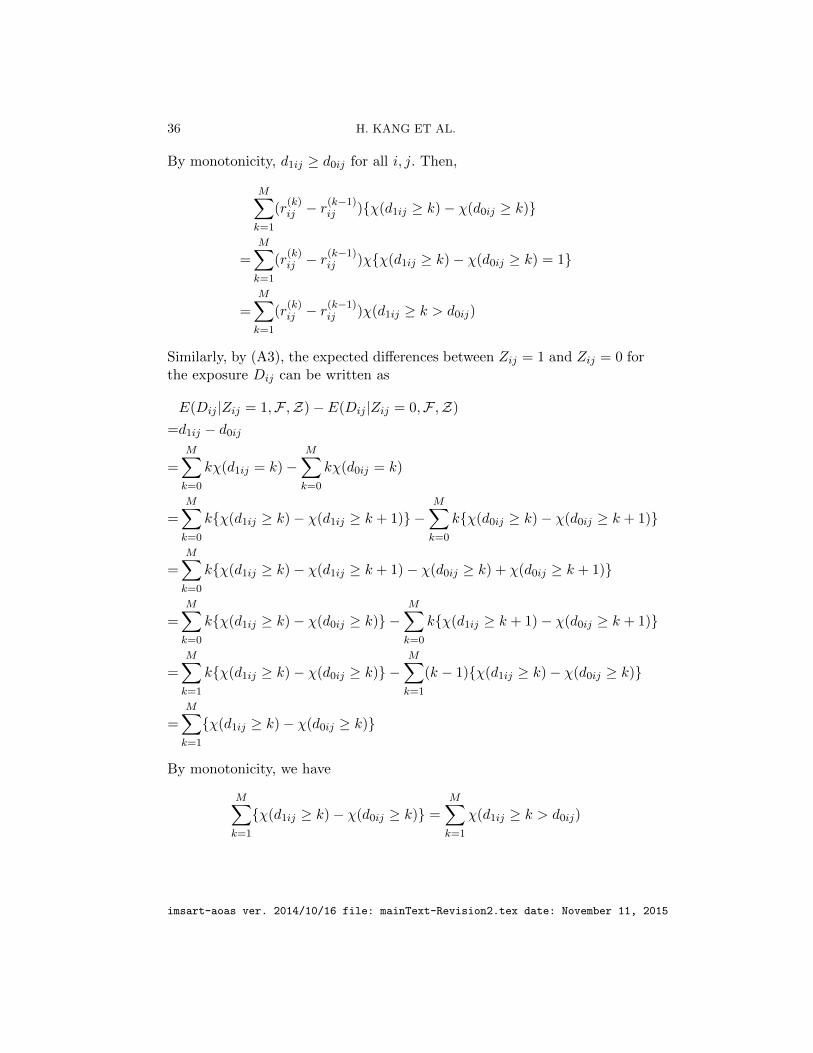
36 H. KANG ET AL.
By monotonicity, d1ij ≥ d0ij for all i, j. Then,
M∑k=1
(r(k)ij − r
(k−1)ij )χ(d1ij ≥ k)− χ(d0ij ≥ k)
=M∑k=1
(r(k)ij − r
(k−1)ij )χχ(d1ij ≥ k)− χ(d0ij ≥ k) = 1
=M∑k=1
(r(k)ij − r
(k−1)ij )χ(d1ij ≥ k > d0ij)
Similarly, by (A3), the expected differences between Zij = 1 and Zij = 0 forthe exposure Dij can be written as
E(Dij |Zij = 1,F ,Z)− E(Dij |Zij = 0,F ,Z)
=d1ij − d0ij
=
M∑k=0
kχ(d1ij = k)−M∑k=0
kχ(d0ij = k)
=M∑k=0
kχ(d1ij ≥ k)− χ(d1ij ≥ k + 1) −M∑k=0
kχ(d0ij ≥ k)− χ(d0ij ≥ k + 1)
=
M∑k=0
kχ(d1ij ≥ k)− χ(d1ij ≥ k + 1)− χ(d0ij ≥ k) + χ(d0ij ≥ k + 1)
=M∑k=0
kχ(d1ij ≥ k)− χ(d0ij ≥ k) −M∑k=0
kχ(d1ij ≥ k + 1)− χ(d0ij ≥ k + 1)
=
M∑k=1
kχ(d1ij ≥ k)− χ(d0ij ≥ k) −M∑k=1
(k − 1)χ(d1ij ≥ k)− χ(d0ij ≥ k)
=M∑k=1
χ(d1ij ≥ k)− χ(d0ij ≥ k)
By monotonicity, we have
M∑k=1
χ(d1ij ≥ k)− χ(d0ij ≥ k) =M∑k=1
χ(d1ij ≥ k > d0ij)
imsart-aoas ver. 2014/10/16 file: mainText-Revision2.tex date: November 11, 2015
FULL MATCHING IV ESTIMATION 37
Thus, we end up with∑Ii=1
∑nij=1E(Rij |Zij = 1,F ,Z)− E(Rij |Zij = 0,F ,Z)∑I
i=1
∑nij=1E(Dij |Zij = 1,F ,Z)− E(Dij |Zij = 0,F ,Z)
=
∑Ii=1
∑nij=1 r
(d1ij)1ij − r(d0ij)
0ij∑Ii=1
∑nij=1 d1ij − d0ij
=
∑Ii=1
∑nij=1
∑Mk=1(r
(k)ij − r
(k−1)ij )χ(d1ij ≥ k > d0ij)∑I
i=1
∑nij=1
∑Mk=1 χ(d1ij ≥ k > d0ij)
APPENDIX C: SUPPLEMENTARY MATERIALS: THEORETICALPROPERTIES OF TEST STATISTIC
Recall the hypothesis of interest from the main manuscript (Section 2.5)
H0 : λ = λ0, Ha : λ 6= λ0
Proposition 2 provides an asymptotic distribution for the test statistic T (λ0)in equation (10) under the null hypothesis H0.
Proposition 2. Assume that for every I, (i) ni remains bounded and
(ii) 1I
∑Ii=1
∑nij=1 r
(d1ij)1ij − r(d0ij)
0ij and 1I
∑Ii=1
∑nij=1 d1ij − d0ij remains fixed
at r and d 6= 0, respectively, so that λ = r/d. In addition, we assume thefollowing moment conditions
(12)I∑i=1
EV 4i (λ)|F ,Z = o(I2), lim sup
I→∞
∑Ii=1E|Vi(λ)− µi,λ|3[∑Ii=1 V arVi(λ)
]3/2= 0
Then, under the null hypothesis H0 : λ = λ, for all t > 0,
lim supI→∞
P
T (λ)
S(λ)≤ −t|F ,Z
≤ Φ(−t), lim sup
I→∞P
T (λ)
S(λ)≥ t|F ,Z
≤ Φ(−t)
where Φ(·) is the standard normal distribution.
To prove Proposition 2, we require the following two Lemmas. Lemma 1characterizes the moments of the test statistics in (10). Lemma 2 derives thebias of S2(λ0) in estimating the variance of T (λ0). Proof of these Lemmasare in Section H of the Supplementary Materials.
imsart-aoas ver. 2014/10/16 file: mainText-Revision2.tex date: November 11, 2015

38 H. KANG ET AL.
Lemma 1. The expected value and the variance of the test statistic inequation (10) are
ET (λ0)|F ,Z =1
I(λ− λ0)
I∑i=1
ni∑j=1
(d1ij − d0ij)
V arT (λ0)|F ,Z =1
I2
I∑i=1
1
ni
ni∑i=1
(aij,λ0 − ai,λ0)2
where
aij,λ0 =nimiy
(d1ij)1ij,λ0
+ni
ni −miy
(d0ij)0ij,λ0
, ai,λ0 =1
ni
ni∑i=1
aij,λ0
Lemma 2. Let µi,λ0 = EVi(λ0)|F ,Z and µλ0 = ET (λ0)|F ,Z. Thebias of (11) in estimating the variance of the test statistic in (10) is
(13) ES2(λ0)|F ,Z − V arT (λ0)|F ,Z =1
I(I − 1)
I∑i=1
(µi,λ0 − µλ0)2
Proof of Proposition 2. We use the same notation adopted in theproof of Lemma 2, mainly µi,λ, µλ, and v2
i,λ. In addition, let qi,λ = EV 2
i (λ)|F ,Z,and vλ = V arT (λ)|F ,Z. First,
∑Ii=1 V
2i (λ)/I is an unbiased estimator for∑I
i=1 qi,λ/I. In addition,
V ar
1
I
I∑i=1
V 2i (λ)|F ,Z
≤ 1
I2
I∑i=1
EV 4i (λ)|F ,Z
By the fourth moment condition in (12), we have∑I
i=1 V2i (λ)/I−
∑Ii=1 qi,λ/I →
0 in probability. Similarly, the same fourth moment condition in (12) andthe same reasoning gives T (λ)−µλ → 0 in probability because of the growthof the variance of T (λ) is controlled by the moment condition. Since µλ = 0for all I under the null hypothesis, we have, by the continuous mappingtheorem, T 2(λ)→ 0 in probability. Combining all these convergence results,we get that for ε > 0 and δ > 0, there exists I∗ such that
for I ≥ I∗:P
1
I
I∑i=1
V 2i (λ)− 1
I
I∑i=1
qi,λ < −ε
2
<δ
2, P
T 2(λ) < − ε
2
<δ
2
imsart-aoas ver. 2014/10/16 file: mainText-Revision2.tex date: November 11, 2015

FULL MATCHING IV ESTIMATION 39
and
PIS2(λ)− Ivλ < −ε
=P
[I
I − 1
1
I
I∑i=1
V 2i (λ)− T 2(λ)
− Ivλ < −ε
]
=P
[I
I − 1
1
I
I∑i=1
V 2i (λ)− 1
I
I∑i=1
qi,λ +1
I
I∑i=1
qi,λ − T 2(λ)
− Ivλ < −ε
]
=P
[I
I − 1
1
I
I∑i=1
V 2i (λ)− 1
I
I∑i=1
qi,λ − T 2(λ)
− Ivλ +
1
I − 1
I∑i=1
qi,λ < −ε
]
≤P
[I
I − 1
1
I
I∑i=1
V 2i (λ)− 1
I
I∑i=1
qi,λ − T 2(λ)
< −ε
]
≤δ2
+δ
2= δ
Stated in words, IS2(λ) will over-estimate Ivλ with high probability.Second, under the null hypothesis H0 : λ = λ and from Lemma 1,∑Ii=1 µi,λ/I = 0. Hence, we can rewrite the test statistic as
T (λ) =1
I
I∑i=1
Vi(λ) =1
I
I∑i=1
[Vi(λ)− µi,λ]
where the test statistic becomes a sum of independent random variablesVi(λ)− µi,λ with mean zero and variance vi,λ.
Finally, combining the two facts, under the null H0 : λ = λ, we have
T (λ)
S(λ)=
1I
∑Ii=1Vi(λ)− µi,λ√
1I2∑I
i=1 vi,λ
√
1I2∑I
i=1 vi,λ√S2(λ)
By conditions specified in Breiman (1992, pg 186) for the central limit the-orem with non-identical distributions, the first parenthesis term convergesto the standard Normal distribution. From our result about IS2
λoveresti-
mating Ivλ, the second parenthesis term will be smaller than 1 with highprobability. Hence, taking the sup of the entire expression, we obtain
lim supI→∞
P
T (λ)
S(λ)≤ −t|F ,Z
≤ Φ(−t), lim sup
I→∞P
T (λ)
S(λ)≥ t|F ,Z
≤ Φ(−t)
where Φ() is the standard normal distribution.
imsart-aoas ver. 2014/10/16 file: mainText-Revision2.tex date: November 11, 2015
40 H. KANG ET AL.
Proposition 2 provides a way to estimate the effect ratio, compute p-values, and calculate confidence intervals. In particular, in the spirit ofHodges and Lehmann (1963), the estimator for the effect ratio, denotedas λ, is the solution to the equation T (λ)/S(λ) = 0. The 95% confidence in-terval for the effect ratio is the solution to the equation T (λ)/S(λ) = ±1.96.Corollary 1 presents a solution to the equation T (λ)/S(λ) = q for any valueof q.
Corollary 1. For any value q, the solution to T (λ)/S(λ) = q is asolution to the quadratic equation A2λ
2 +A1λ+A0 = 0 where
A2 = H2. −
q2
I(I − 1)
I∑i=1
(Hi − H.)2
A1 = −2G.H. +2q2
I(I − 1)
I∑i=1
(Gi − G.)(Hi − H.)
A0 = G2. −
q2
I(I − 1)
I∑i=1
(Gi − G.)2
where
Gi =n2i
mi(ni −mi)
ni∑j=1
(Zij − Zi.)(Rij − Ri.)
Hi =n2i
mi(ni −mi)
ni∑j=1
(Zij − Zi.)(Dij − Di.)
Zi. =1
ni
ni∑j=1
Zij , Di. =1
ni
ni∑j=1
Dij , Ri. =1
ni
ni∑j=1
Rij
H. =1
I
I∑i=1
Hi, G. =1
I
I∑i=1
Gi
Proof. First, we see that T (λ)/S(λ) = q implies T 2(λ) = q2S2(λ). Thisexpression can be rewritten as(14)
T 2(λ) =q2
I(I − 1)
I∑i=1
(Vi(λ)− T (λ))2 =q2
I(I − 1)
I∑i=1
V 2i (λ)− IT 2(λ)
imsart-aoas ver. 2014/10/16 file: mainText-Revision2.tex date: November 11, 2015
FULL MATCHING IV ESTIMATION 41
Rearranging the terms in (14), we get
T 2(λ)
(1 +
q2
I − 1
)=
q2
I(I − 1)
I∑i=1
V 2i (λ)
Second, we can re-express Vi(λ) as follows.
Vi(λ) =
ni∑j=1
(nimi
+ni
ni −mi
)ZijRij −
ni∑j=1
nini −mi
Rij
−ni∑j=1
(nimi
+ni
ni −mi
)λZijDij +
ni∑j=1
nini −mi
λDij
=
ni∑j=1
n2i
mi(ni −mi)ZijRij −
ni∑j=1
nini −mi
Rij
1
mi
ni∑j=1
Zij
−
ni∑j=1
n2i
mi(ni −mi)λZijDij +
ni∑j=1
nini −mi
λDij
1
mi
ni∑j=1
Zij
=
n2i
mi(ni −mi)
ni∑j=1
ZijRij −1
ni
ni∑j=1
Rij
ni∑j=1
Zij
− λ n2
i
mi(ni −mi)
ni∑j=1
ZijDij −1
ni
ni∑j=1
Dij
ni∑j=1
Zij
=
n2i
mi(ni −mi)
ni∑j=1
(Zij − Zi.)(Rij − Ri.)− λn2i
mi(ni −mi)
ni∑j=1
(Zij − Zi.)(Dij − Di.)
Immediately, we also have Vi(λ) = Gi−λHi. Then, we can rewrite∑I
i=1 V2i (λ)
imsart-aoas ver. 2014/10/16 file: mainText-Revision2.tex date: November 11, 2015

42 H. KANG ET AL.
and T 2(λ) as follows
I∑i=1
V 2i (λ) =
I∑i=1
(Gi − λHi)2
=
I∑i=1
G2i − 2λ
I∑i=1
GiHi + λ2I∑i=1
H2i
T 2(λ) =1
I2
I∑i=1
Vi(λ)
2
=1
I2
I∑i=1
(Gi − λHi)
2
=1
I2
(
I∑i=1
Gi
)2
− 2λI∑i=1
Gi
I∑i=1
Hi + λ2
(I∑i=1
Hi
)2
Overall, we can rewrite the equation (14) as
1
I2
(
I∑i=1
Gi
)2
− 2λ
I∑i=1
Gi
I∑i=1
Hi + λ2
(I∑i=1
Hi
)2(
1 +q2
I − 1
)
=q2
I(I − 1)
(I∑i=1
G2i − 2λ
I∑i=1
GiHi + λ2I∑i=1
H2i
)
Finally, we pull out the coefficients associated with λ2 and λ, denoted as A2
and A1, respectively. The remaining term are constants and we denote them
imsart-aoas ver. 2014/10/16 file: mainText-Revision2.tex date: November 11, 2015
FULL MATCHING IV ESTIMATION 43
as A0. All A2, A1, and A0 are explicitly written below.
A2 =1
I2
(I∑i=1
Hi
)2
+q2
I(I − 1)
1
I
(I∑i=1
Hi
)2
−I∑i=1
H2i
= H2
. −q2
I(I − 1)
I∑i=1
(Hi − H.)2
A1 = −2
[1
I2
I∑i=1
Gi
I∑i=1
Hi +q2
I(I − 1)
1
I
I∑i=1
Gi
I∑i=1
Hi −I∑i=1
GiHi
]
= −2
[G.H. −
q2
I(I − 1)
I∑i=1
(Gi − G.)(Hi − H.)
]
A0 =1
I2
(I∑i=1
Gi
)2
+q2
I(I − 1)
1
I
(I∑i=1
Gi
)2
−I∑i=1
G2i
= G2
. −q2
I(I − 1)
I∑i=1
(Gi − G.)2
If q = 0 in Corollary 1, there is only one solution to the quadratic equationsince
A2λ2 +A1λ+A0 = H2
. λ2 − 2H.G.λ+ G2
. = (H.λ− G.)2 = 0
This gives us an explicit formula for the estimator of the effect ratio, denotedas λ.
(15) λ =G.H.
=
∑Ii=1
n2i
mi(ni−mi)
∑nij=1(Rij − Ri.)(Zij − Zi.)∑I
i=1n2i
mi(ni−mi)
∑nij=1(Dij − Di.)(Zij − Zi.)
APPENDIX D: SUPPLEMENTARY MATERIALS: SENSITIVITYANALYSIS
To model this deviation from randomized assignment due to unmeasuredconfounders, let πij = P (Zij = 1|F) and πik = P (Zik = 1|F) for each unit jand k in the ith matched set. The odds that unit j will receive Zij = 1 insteadof Zij = 0 is πij/(1 − πij). Similarly, the odds for unit k is πik/(1 − πik).Suppose the ratio of these odds is bounded by Γ ≥ 1
(16)1
Γ≤ πij(1− πik)πik(1− πij)
≤ Γ
imsart-aoas ver. 2014/10/16 file: mainText-Revision2.tex date: November 11, 2015

44 H. KANG ET AL.
If unmeasured confounders play no role in the assignment of Zij , Γ = 1and πij = πik. That is, child j and k have the same probability of receivingZij = 1 in matched set i. If there are unmeasured confounders that affectthe distribution of Zij , then πij 6= πik and Γ > 1. By Rosenbaum (2002),equation (16) is equivalent to
(17) P (Z = z|F ,Z) =exp(γzTu)∑b∈Ω exp(γbTu)
where u = (u11, u12, ..., uInI). Unfortunately, the exact probability of (17) is
unknown as it depends on the vector of unobserved confounders, (u11, . . . , uInI).
However, for a fixed Γ > 1, we can obtain lower and upper bounds on (17).Furthermore, since the inference on the effect ratio λ is derived from the dis-tribution of P (Z = z|F ,Z), these bounds can be used to compute a rangeof possible p-values under the null hypothesis. The range of p-values indi-cates the effect of unmeasured confounders on the conclusions reached bythe inference on λ. If the range contains α, the significance value, then wecannot reject the null hypothesis at the α level when there is an unmeasuredconfounder with an effect quantified by Γ.
Specifically, consider Fisher’s sharp null hypothesis, H0 : r(d1ij)1ij = r
(d0ij)0ij
for all i = 1, . . . , n and j = 1, . . . , ni. Note that this hypothesis implies thehypothesis H0 : λ = 0. Furthermore, the test statistic in (10) simplifies to
T (0) =1
I
I∑i=1
nimi
ni∑j=1
ZijRij −ni
ni −mi
ni∑j=1
(1− Zij)Rij
=
1
I
I∑i=1
n2i
mi(ni −mi)
ni∑j=1
ZijRij −1
I
I∑i=1
nini −mi
ni∑j=1
Rij
Regardless of the distribution of P (Z = z|F ,Z), 1I
∑Ii=1 ni/(ni−mi)
∑nij=1Rij
is a constant since r(d1ij)1ij = r
(d0ij)0ij under Fisher’s sharp null hypothesis.
Hence, we can use the simpler statistic, T (0),
(18) T (0) =1
I
I∑i=1
nimi(ni −mi)
ni∑j=1
ZijRij
to test the Fisher’s sharp null hypothesis. If the responses are binary, equa-tion (18) is the sign-score test statistic for which exact bounds on p-valuesexist (Rosenbaum, 2002). If the responses are continuous, Gastwirth et al.(2000) and Small et al. (2009) provide an approximate bound on p-values.
imsart-aoas ver. 2014/10/16 file: mainText-Revision2.tex date: November 11, 2015
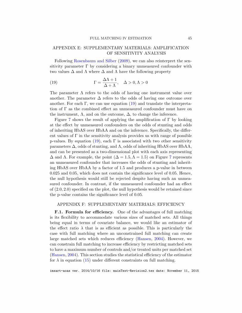
FULL MATCHING IV ESTIMATION 45
APPENDIX E: SUPPLEMENTARY MATERIALS: AMPLIFICATIONOF SENSITIVITY ANALYSIS
Following Rosenbaum and Silber (2009), we can also reinterpret the sen-sitivity parameter Γ by considering a binary unmeasured confounder withtwo values ∆ and Λ where ∆ and Λ have the following property
(19) Γ =∆Λ + 1
∆ + Λ, ∆ > 0,Λ > 0
The parameter Λ refers to the odds of having one instrument value overanother. The parameter ∆ refers to the odds of having one outcome overanother. For each Γ, we can use equation (19) and translate the interpreta-tion of Γ as the combined effect an unmeasured confounder must have onthe instrument, Λ, and on the outcome, ∆, to change the inference.
Figure 7 shows the result of applying the amplification of Γ by lookingat the effect by unmeasured confounders on the odds of stunting and oddsof inheriting HbAS over HbAA and on the inference. Specifically, the differ-ent values of Γ in the sensitivity analysis provides us with range of possiblep-values. By equation (19), each Γ is associated with two other sensitivityparameters ∆, odds of stunting, and Λ, odds of inheriting HbAS over HbAA,and can be presented as a two-dimensional plot with each axis representing∆ and Λ. For example, the point (∆ = 1.5,Λ = 1.5) on Figure 7 representsan unmeasured confounder that increases the odds of stunting and inherit-ing HbAS over HbAA by a factor of 1.5 and produces a p-value in between0.025 and 0.05, which does not contain the significance level of 0.05. Hence,the null hypothesis would still be rejected despite having such an unmea-sured confounder. In contrast, if the unmeasured confounder had an effectof (2.0, 2.0) specified on the plot, the null hypothesis would be retained sincethe p-value contains the significance level of 0.05.
APPENDIX F: SUPPLEMENTARY MATERIALS: EFFICIENCY
F.1. Formula for efficiency. One of the advantages of full matchingis its flexibility to accommodate various sizes of matched sets. All thingsbeing equal in terms of covariate balance, we would like an estimator ofthe effect ratio λ that is as efficient as possible. This is particularly thecase with full matching where an unconstrained full matching can createlarge matched sets which reduces efficiency (Hansen, 2004). However, wecan constrain full matching to increase efficiency by restricting matched setsto have a maximum number of controls and/or treated units per matched set(Hansen, 2004). This section studies the statistical efficiency of the estimatorfor λ in equation (15) under different constraints on full matching.
imsart-aoas ver. 2014/10/16 file: mainText-Revision2.tex date: November 11, 2015
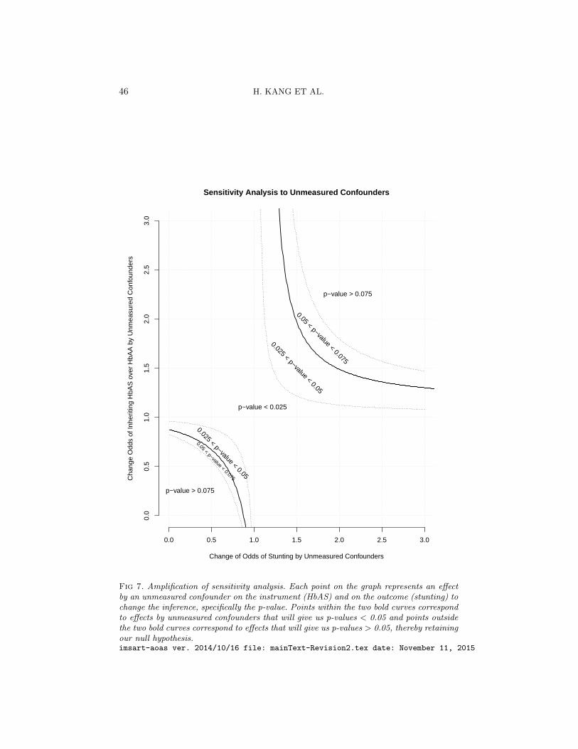
46 H. KANG ET AL.
Sensitivity Analysis to Unmeasured Confounders
Change of Odds of Stunting by Unmeasured Confounders
Cha
nge
Odd
s of
Inhe
ritin
g H
bAS
ove
r H
bAA
by
Unm
easu
red
Con
foun
ders
0.0 0.5 1.0 1.5 2.0 2.5 3.0
0.0
0.5
1.0
1.5
2.0
2.5
3.0
p−value < 0.025
0.025 < p−value < 0.05
0.05 < p−value < 0.075
p−value > 0.075
0.025 < p−value < 0.05
0.05 < p−value < 0.075
p−value > 0.075
Fig 7. Amplification of sensitivity analysis. Each point on the graph represents an effectby an unmeasured confounder on the instrument (HbAS) and on the outcome (stunting) tochange the inference, specifically the p-value. Points within the two bold curves correspondto effects by unmeasured confounders that will give us p-values < 0.05 and points outsidethe two bold curves correspond to effects that will give us p-values > 0.05, thereby retainingour null hypothesis.imsart-aoas ver. 2014/10/16 file: mainText-Revision2.tex date: November 11, 2015
FULL MATCHING IV ESTIMATION 47
To study the efficiency of the effect ratio estimator for different ni andmi, we study a simple version of the structural equations model introducedpopular in econometrics and has been used to study the properties of 2SLS,the most popular IV estimator (Wooldridge, 2010). Let (Rij , Dij , Zij) bei.i.d. observations from an infinite population under the following model.
Rij = αi + βDij + εij , E(εij |Zij) = 0(20)
Dij = τi + γZij + ξij , E(ξij |Zij) = 0(21)
with the following moment conditions.
V ar(εij |Zij) = σ2i,R, V ar(ξij |Zij) = σ2
i,D, E(εijξij |Zij) = σi,RD
The parameters αi, i = 1, . . . , I measure the effect on the outcome frombeing in matched set i. The parameter β is the effect of interest, the effectof the exposure on the outcome. Note that the treatment effect in (20)is assumed to be homogeneous for everyone, which is not assumed in themain manuscript. The parameters τi, i = 1, . . . , I measure the effect on theexposure from being in matched set i. The parameter γ is the effect of theinstrument on the exposure. By including αi and τi, the models (20) and(21) incorporate the matching aspect of IV estimation since each matchedset i have effects on Rij and Dij that are unique to that matched set.
The effect ratio, λ, is related to parameters found in standard structuralequation models in (20) and (21). To illustrate this, note that the poten-tial outcomes notation can be rewritten under the models (20) and (21) asfollows.
Rij =
r
(d1ij)1ij = αi + βτi + βγ + βξij + εij if Zij = 1
r(d0ij)0ij = αi + βτi + βξij + εij if Zij = 0
Dij =
d1ij = τi + γ + ξij if Zij = 1
d0ij = τi + ξij if Zij = 0
Then, the effect ratio in (9) turns out to be
λ =
∑Ii=1
∑nij=1 r
(d1ij)1ij − r(d0ij)
0ij∑Ii=1
∑nij=1 d1ij − d0ij
=
∑Ii=1
∑nij=1 βγ∑I
i=1
∑nij=1 γ
=βγ
γ= β
Hence, λ = β and because of this equivalence, inferences for the effect ratioprovides inference for β.
Thus, the parameter β can be estimated by the effect ratio estimatordiscussed in Section C of the Supplementary Materials, specifically equation
imsart-aoas ver. 2014/10/16 file: mainText-Revision2.tex date: November 11, 2015
48 H. KANG ET AL.
(15),
β =
∑Ii=1
n2i
mi(ni−mi)
∑nij=1(Zij − Zi.)(Rij − Ri.)∑I
i=1n2i
mi(ni−mi)
∑nij=1(Zij − Zi.)(Dij − Di.)
Proposition 3 computes the asymptotic variance of β to study the efficiencyof the effect ratio estimator.
Proposition 3. Suppose we have models (20) and (21) with γ 6= 0 andthe third moment of εij is bounded for all i, j. Define the following variables
Ji =
ni∑j=1
(Zij − Zi.)(εij − εi.), Hi =
ni∑j=1
(Zij − Zi.)(Dij − Di.), εi. =1
ni
ni∑j=1
εij
s2I =
I∑i=1
n3i
mi(ni −mi)σ2i,R
Assume that (i) Zij are fixed, (ii) ni remain bounded for all i, and thefollowing moment conditions are met for Ji and Hi
lim supI→∞
1
s3I
I∑i=1
n6i
m3i (ni −mi)3
E(|Ji|3) = 0,I∑i=1
V ar
(n2i
mi(ni −mi)H2i
)= o(I2)
Then, the asymptotic variance of the effect ratio estimator in (15) is
√I(β − β)→ N
0,
(limI→∞
sI√I
)2
γ2(
limI→∞1I
∑Ii=1 ni
)2
Proof of Proposition 3. First, for all i = 1, . . . , I and j = 1, . . . , ni,
we have
Zij − Zi. =
1− mi
niif Zij = 1
−mini
if Zij = 0
Furthermore,
ni∑j=1
(Zij − Zi.) = 0,
ni∑j=1
(Zij − Zi.)2 =mi(ni −mi)
ni
imsart-aoas ver. 2014/10/16 file: mainText-Revision2.tex date: November 11, 2015
FULL MATCHING IV ESTIMATION 49
Second, for fixed Zij , we have the following expected values for Ji
E(Ji) =0
E(J2i ) =V ar
ni∑j=1
(Zij − Zi.)(εij − εi.)
=
ni∑j=1
(Zij − Zi.)2V ar(εij − εi.) +∑j,k
(Zij − Zi.)(Zik − Zk.)Cov(εij − εi., εik − εi.)
=(1− 1
ni)σ2i,R
ni∑j=1
(Zij − Zi.)2 − 1
niσ2i,R
∑j,k
(Zij − Zi.)(Zik − Zk.)
=σ2i,R
ni∑j=1
(Zij − Zi.)2 − 1
niσ2i,R
ni∑j=1
(Zij − Zi.)
2
=σ2i,R
mi(ni −mi)
ni
For the third moment, for each i, let k1, . . . , kni be non-negative integersand define the multinomial coefficient as follows.(
3
k1, . . . , kni
)=
3!
k1! · · · kni !
Then, we have
E(|J3i |) =E|
ni∑j=1
(Zij − Zi.)(εij − εi.)
3
|
=E|∑
k1+···+kni=3
(3
k1, . . . , kni
) ni∏j=1
(Zij − Zi.)(εij − εi.)
kj |≤
∑k1+···+kni=3
(3
k1, . . . , kni
) ni∏j=1
|Zij − Zi.|kjE|εij − εi.|kj <∞
because third moments exist and are bounded for all εij and ni is bounded.Third, based on these moment calculations, it immediately follows that
E
[I∑i=1
n2i
(mi)(ni −mi)Ji
2]
=
I∑i=1
n4i
(mi)2(ni −mi)2
mi(ni −mi)
niσ2i,R
= s2
I
imsart-aoas ver. 2014/10/16 file: mainText-Revision2.tex date: November 11, 2015
50 H. KANG ET AL.
Then, by Theorem 9.2 in Chapter 9, Section 3 of Breiman (1992) (pg 187),the sum of Ji weighted by n2
i /mi(ni−mi) is a standard Normal distribution∑Ii=1
n2i
mi(ni−mi)Ji
sI→ N(0, 1)
Fourth, for Hi, we have the following moments
E(Hi) =γmi(1−mi
ni)
V ar(Hi) =V ar
ni∑j=1
(Zij − Zi.)(Dij − Di.)
=(1− 1
ni)σ2i,D
ni∑j=1
(Zij − Zi.)2 − 1
niσ2i,D
∑j,k
(Zij − Zi.)(Zik − Zk.)
=σ2i,D
ni∑j=1
(Zij − Zi.)2 − 1
niσ2i,D
ni∑j=1
(Zij − Zi.)
2
=σ2i,D
mi(ni −mi)
ni
Fifth, by Theorem C in page 27 of Serfling (1980),
1
I
I∑i=1
n2i
mi(ni −mi)Hi − γ
1
I
I∑i=1
E
n2i
mi(ni −mi)Hi
=1
I
I∑i=1
n2i
mi(ni −mi)Hi − γ
1
I
I∑i=1
ni → 0
Finally, combining all these facts together, we can rewrite the effect ratioestimator as follows.
β =
∑Ii=1
n2i
mi(ni−mi)
∑nij=1(Zij − Zi.)(Rij − Ri.)∑I
i=1n2i
mi(ni−mi)
∑nij=1(Zij − Zi.)(Dij − Di.)
= β +
∑Ii=1
n2i
mi(ni−mi)
∑nij=1(Zij − Zi.)(εij − εi.)∑I
i=1n2i
mi(ni−mi)Hi
= β +
∑Ii=1
n2i
mi(ni−mi)Ji∑I
i=1n2i
mi(ni−mi)Hi
imsart-aoas ver. 2014/10/16 file: mainText-Revision2.tex date: November 11, 2015

FULL MATCHING IV ESTIMATION 51
which leads to
√I(β − β) =
∑I
i=1n2i
mi(ni−mi)Ji
sI
1√IsI
1I
∑Ii=1
n2i
mi(ni−mi)Hi
Finally, using Slutsky’s Theorem,
√I(β − β) converges to a Normal distri-
bution with mean 0 and stated asymptotic variance.
Proposition 3 provides an easy way to compare between different types offull matching methods and their effect on the estimation of the effect ratio.For example, in the simple case of homoscedastic variance, the approximatevariance of λ is
V ar(λ) ≈ K∑I
i=1n3i
ni−1(∑Ii=1 ni
)2
where K is some constant that depends on the variance of Rij and thestrength of the instrument. Since K will be identical for all full matcheddesigns, we can simply look at the quantities to the right of K to tweak ourfull matching algorithm to produce the most efficient estimator.
With regards to the quality of the approximation, the asymptotic vari-ance is a decent approximation to the estimator’s variance if the number ofmatched sets, I, are large or if the instruments are strong. This is demon-strated in Table 4 which is a result of the following simulation study. Thevariables Rij , Dij and Zij are generated via the model in (20) and (21) withZij assumed to be fixed. We randomly pick αi, τi, and β. We pick γ to be 1for the strong instrument case and −0.2 for the weak instrument case. Weassume a homoscedastic variance for the error terms where all the σ2
i,R, σ2i,D,
and σi,RD are the same for every i. We compute the effect ratio estimator,repeat this process 1000 times, and compute the simulated variance. Thetheoretical variance is calculated based on the formula provided in Proposi-tion 3.
Table 4 shows us that for strong instruments, the agreement betweentheoretical formula in Proposition 3 and simulation is quite good for allvalues of I. On the other hand, for weak instruments, there is substantialdeviation between the theoretical variance and the simulated variance untilI is above 5000.
F.2. Simulation to approximate efficiency. The prior section offersa formula to compute efficiency of various full matching schemes. However,for the formula to be valid, it requires, among other things, a linear model
imsart-aoas ver. 2014/10/16 file: mainText-Revision2.tex date: November 11, 2015

52 H. KANG ET AL.
Table 4Comparison of simulated variance and theoretical variance for different strength of
instruments and matched set number I.
I Theoretical Variance Simulated VarianceStrong Weak Strong Weak
50 0.024 0.59 0.028 3224.30100 0.012 0.30 0.012 181.06110 0.011 0.27 0.012 2506.92500 0.0024 0.060 0.0025 2.051000 0.0012 0.030 0.0012 0.0375000 0.00024 0.0060 0.00024 0.006310000 0.00012 0.0030 0.00012 0.0030
between the outcome, Rij and the exposureDij . In our study where stunting,the outcome, is a binary variable and malaria, the exposure, is a wholenumber, it is unreasonable to assume that Rij is a linear function of Dij .
In such cases, we propose a simulation study to analyze efficiency fordifferent full matching schemes. As an illustration, consider our study withthe effect of malaria on stunting. For each matching scheme, we fix Zij andXij , which, in turn, fixes the matched sets. For the other variables, Dij andRij , we assume a Poisson relationship between Dij and Zij and a logisticrelationship between Dij and Rij . In particular, we use the following model
P (Rij = 1) =1
1 + e−(αi+βDij+uij), E(Dij) = eτi+γZij
We fix β, the effect of malaria on stunting, to be 0.32 and γ, the strength ofthe instrument, to be −0.20 based on the estimates in Kang et al. (2013); theestimate of γ was based on the risk ratio estimate. We also randomly chooseαi and τi, the intercepts, from Normal distributions with means −1.67 and−0.19, respectively, and variances 0.12 and 0.027, respectively. The meanand the variance for αi is from the intercept term and its correspondingstandard error of the logistic regression between Rij and Dij . Similarly, themean and the variance for τi is from the intercept term and its correspondingstandard error of the Poisson regression between Dij and Zij . Once all theparameters are set, we sample 884 observations of (Rij , Dij) (i.e. the samplesize of the malaria data set) and compute the effect ratio estimator basedon the sample of 884. Note that the effect ratio estimator should be able toestimate β since it doesn’t rely on the functional form between stunting (i.e.outcome) and malaria episodes (i.e. exposure). We repeat the simulation5000 times and compute the median absolute deviation as a robust proxyfor variance of the effect ratio estimator.
Table 5 shows the trade-off between efficiency and covariate balance for
imsart-aoas ver. 2014/10/16 file: mainText-Revision2.tex date: November 11, 2015

FULL MATCHING IV ESTIMATION 53
Table 5Trade-off between efficiency and balance for different full matching schemes that use allthe data based on simulation based on median absolute deviation and standardized bias.
Matching Median absolute deviation Standardized bias
Full matching (max strata size is 9) 0.90 0.23Full matching (max strata size is 10) 0.96 0.19Full matching (max strata size is 15) 0.97 0.10Full matching (unrestricted) 0.98 0.055
different full matching schemes that use all 884 samples of the malaria data.In particular, we restrict the matched set sizes to different values to see theirimpact on efficiency and standardized bias. The standardized bias is the in-strumental propensity score (Cheng, 2011) and is calculated as the differencein propensity scores before and after matching normalized by the withingroup standard deviation before matching (the square root of the averageof the variances within the group). We see that unrestricted full matchinghas the lowest bias among all other full matching schemes. However, fullmatching with restricted strata size of 9 has the lowest median absolute de-viation, albeit by a little in comparison to other matching schemes. Giventhe large bias reduction by using unrestricted full matching with a smallgain in median absolute deviation, we use unrestricted full matching in ourmain manuscript.
APPENDIX G: SUPPLEMENTARY MATERIALS: EXTENDEDSIMULATION
G.1. Strength of instruments. The simulation setup is identical tothe one in Section 3 of the main manuscript. We present another aspectof our estimator’s performance in relation to 2SLS, specifically the medianabsolute deviation (MAD). Figure 8 measures the MAD of 2SLS and ourmethod. Our method tends to have a slightly higher MAD than 2SLS. Thishigher variability of our method is to be expected since our method uses anonparametric approach whereas 2SLS is a parametric approach. However,as the instrument gets stronger (i.e. high concentration parameter), the gapbetween the two MADs shrinks quickly.
G.2. Sample size. The simulation result presented here has the iden-tical setup as the one in Section 3 of the main manuscript. However, we fixthe strength of the instrument to be very strong, but vary the sample size.We keep the ratio between Zij = 1 to Zij = 0 to be 1 to 7, respectively.We compare the performance of 2SLS and our method with respect to bias,variance, and type I error rate as we vary f(·).
imsart-aoas ver. 2014/10/16 file: mainText-Revision2.tex date: November 11, 2015
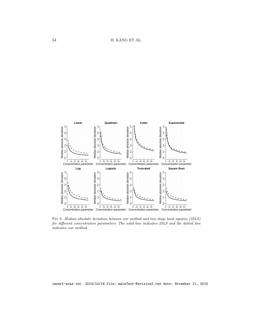
54 H. KANG ET AL.
Linear
Concentration parameter
Med
ian
abso
lute
dev
iatio
n
0 10 20 30 40 50
0.0
0.2
0.4
0.6
0.8
1.0
Quadratic
Concentration parameter
Med
ian
abso
lute
dev
iatio
n
0 10 20 30 40 50
0.0
0.2
0.4
0.6
0.8
1.0
Cubic
Concentration parameter
Med
ian
abso
lute
dev
iatio
n
0 10 20 30 40 50
0.0
0.2
0.4
0.6
0.8
1.0
Exponential
Concentration parameterM
edia
n ab
solu
te d
evia
tion
0 10 20 30 40 500.
00.
20.
40.
60.
81.
0
Log
Concentration parameter
Med
ian
abso
lute
dev
iatio
n
0 10 20 30 40 50
0.0
0.2
0.4
0.6
0.8
1.0
Logistic
Concentration parameter
Med
ian
abso
lute
dev
iatio
n
0 10 20 30 40 50
0.0
0.2
0.4
0.6
0.8
1.0
Truncated
Concentration parameter
Med
ian
abso
lute
dev
iatio
n
0 10 20 30 40 50
0.0
0.2
0.4
0.6
0.8
1.0
Square Root
Concentration parameter
Med
ian
abso
lute
dev
iatio
n
0 10 20 30 40 50
0.0
0.2
0.4
0.6
0.8
1.0
Fig 8. Median absolute deviation between our method and two stage least squares (2SLS)for different concentration parameters. The solid line indicates 2SLS and the dotted lineindicates our method.
imsart-aoas ver. 2014/10/16 file: mainText-Revision2.tex date: November 11, 2015

FULL MATCHING IV ESTIMATION 55
Linear
Sample size
Abs
olut
e bi
as
100 400 700 1000
0.00
0.05
0.10
0.15
0.20
0.25
0.30
Quadratic
Sample size
Abs
olut
e bi
as
100 400 700 1000
0.00
0.05
0.10
0.15
0.20
0.25
0.30
Cubic
Sample size
Abs
olut
e bi
as
100 400 700 1000
0.00
0.05
0.10
0.15
0.20
0.25
0.30
Exponential
Sample sizeA
bsol
ute
bias
100 400 700 1000
0.00
0.05
0.10
0.15
0.20
0.25
0.30
Log
Sample size
Abs
olut
e bi
as
100 400 700 1000
0.00
0.05
0.10
0.15
0.20
0.25
0.30
Logistic
Sample size
Abs
olut
e bi
as
100 400 700 1000
0.00
0.05
0.10
0.15
0.20
0.25
0.30
Truncated
Sample size
Abs
olut
e bi
as
100 400 700 1000
0.00
0.05
0.10
0.15
0.20
0.25
0.30
Square Root
Sample size
Abs
olut
e bi
as
100 400 700 1000
0.00
0.05
0.10
0.15
0.20
0.25
0.30
Fig 9. Absolute bias of the median between our method and two stage least squares (2SLS)for different sample sizes. The solid line indicates 2SLS and the dotted line indicates ourmethod.
imsart-aoas ver. 2014/10/16 file: mainText-Revision2.tex date: November 11, 2015
56 H. KANG ET AL.
Figure 9 measures the absolute bias of 2SLS and our method. When f(·)is a linear function of the observed covariates xij , 2SLS does better thanour method, which is to be expected since 2SLS works best when the modelis linear. However, if f(·) is non-linear, our matching estimator does betterthan 2SLS and is never substantially worse. For example, for quadratic,cubic, exponential, log, and square root functions, our method has lowerbias than 2SLS for all sample size. For logistic and truncated functions, ourmethod is similar in performance to 2SLS.
Figure 10 measures the median absolute deviation (MAD) of 2SLS andour method. Our method tends to have a slightly higher MAD than 2SLS.This higher variability of our method is to be expected since our methoduses a nonparametric approach whereas 2SLS is a parametric approach.
Finally, Figure 11 measures the Type I error rate of 2SLS and our method.Regardless of the function type and and sample size, our method retains thenominal 0.05 rate. In fact, even for the linear case where 2SLS is designedto excel, our estimator has the correct Type I error rate for all sample sizewhile 2SLS has higher Type I error for small sample size. For all the non-linear functions, the Type I error rate for 2SLS remains above the 0.05 line,with the notable exception of logistic and truncated functions whose 2SLSestimators has similar Type I error as our method. In contrast, our estimatormaintains the nominal Type I error rate for all sample sizes. This providesevidence that our estimator will have the correct 95% coverage for confidenceintervals regardless of the non-linearity or for different sample size.
G.3. Comparison to Frolich (2007). In this section, we provide afew additional details of our matching estimator to another non-parametricIV estimator with covariates explored by Frolich (2007) as presented in themain manuscript. The simulation setup is designed to mimic the data typein the malaria data where we have a binary Zij , discrete Dij taking onvalues 0, 1 and 2, and a continuous response Rij and is identical to the onepresented in the main manuscript. Specifically, we have
Rij = α+ βDij + f(Xij) + Uij + εij
Dij = χ(D∗ij < −1) + 2χ(−1 ≤ D∗ij < 1) + 3χ(1 ≤ D∗ij)D∗ij = κ+ πZij + ρTXij + Uij + ξij
where D∗ij is a latent variable, Uij serve as the unmeasured confounder, andεij , ξij , Uij are all i.i.d Normal. Covariates Xij are generated similar to thesimulation study in the main manuscript. As before, we look at bias andvariance across different strengths of instruments, different sample size, anddifferent functions f(·). Similar to the main manuscript, we use the default
imsart-aoas ver. 2014/10/16 file: mainText-Revision2.tex date: November 11, 2015
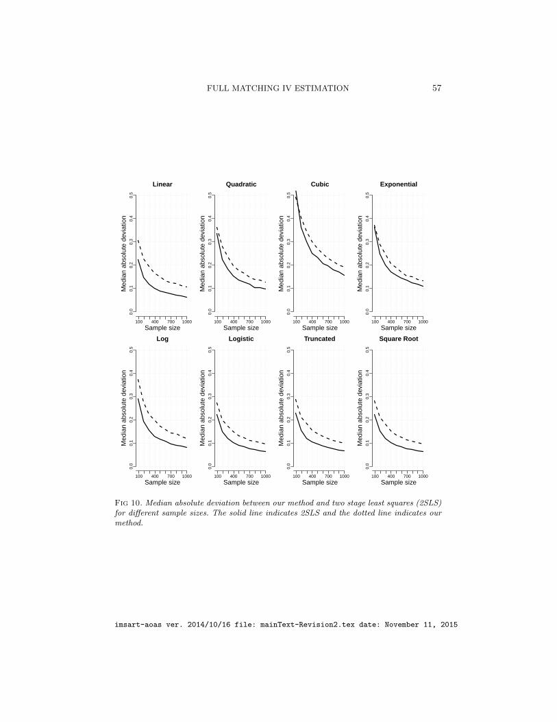
FULL MATCHING IV ESTIMATION 57
Linear
Sample size
Med
ian
abso
lute
dev
iatio
n
100 400 700 1000
0.0
0.1
0.2
0.3
0.4
0.5
Quadratic
Sample size
Med
ian
abso
lute
dev
iatio
n
100 400 700 1000
0.0
0.1
0.2
0.3
0.4
0.5
Cubic
Sample size
Med
ian
abso
lute
dev
iatio
n
100 400 700 1000
0.0
0.1
0.2
0.3
0.4
0.5
Exponential
Sample size
Med
ian
abso
lute
dev
iatio
n
100 400 700 1000
0.0
0.1
0.2
0.3
0.4
0.5
Log
Sample size
Med
ian
abso
lute
dev
iatio
n
100 400 700 1000
0.0
0.1
0.2
0.3
0.4
0.5
Logistic
Sample size
Med
ian
abso
lute
dev
iatio
n
100 400 700 1000
0.0
0.1
0.2
0.3
0.4
0.5
Truncated
Sample size
Med
ian
abso
lute
dev
iatio
n
100 400 700 1000
0.0
0.1
0.2
0.3
0.4
0.5
Square Root
Sample size
Med
ian
abso
lute
dev
iatio
n
100 400 700 1000
0.0
0.1
0.2
0.3
0.4
0.5
Fig 10. Median absolute deviation between our method and two stage least squares (2SLS)for different sample sizes. The solid line indicates 2SLS and the dotted line indicates ourmethod.
imsart-aoas ver. 2014/10/16 file: mainText-Revision2.tex date: November 11, 2015

58 H. KANG ET AL.
Linear
Sample size
Type
I E
rror
Rat
e
100 400 700 1000
0.0
0.1
0.2
0.3
0.4
0.5
Quadratic
Sample size
Type
I E
rror
Rat
e
100 400 700 1000
0.0
0.1
0.2
0.3
0.4
0.5
Cubic
Sample size
Type
I E
rror
Rat
e
100 400 700 1000
0.0
0.1
0.2
0.3
0.4
0.5
Exponential
Sample size
Type
I E
rror
Rat
e
100 400 700 1000
0.0
0.1
0.2
0.3
0.4
0.5
Log
Sample size
Type
I E
rror
Rat
e
100 400 700 1000
0.0
0.1
0.2
0.3
0.4
0.5
Logistic
Sample size
Type
I E
rror
Rat
e
100 400 700 1000
0.0
0.1
0.2
0.3
0.4
0.5
Truncated
Sample size
Type
I E
rror
Rat
e
100 400 700 1000
0.0
0.1
0.2
0.3
0.4
0.5
Square Root
Sample size
Type
I E
rror
Rat
e
100 400 700 1000
0.0
0.1
0.2
0.3
0.4
0.5
Fig 11. Type I error rate between our method and two stage least squares (2SLS) fordifferent sample sizes. The solid line indicates 2SLS and the dotted line indicates ourmethod.
imsart-aoas ver. 2014/10/16 file: mainText-Revision2.tex date: November 11, 2015
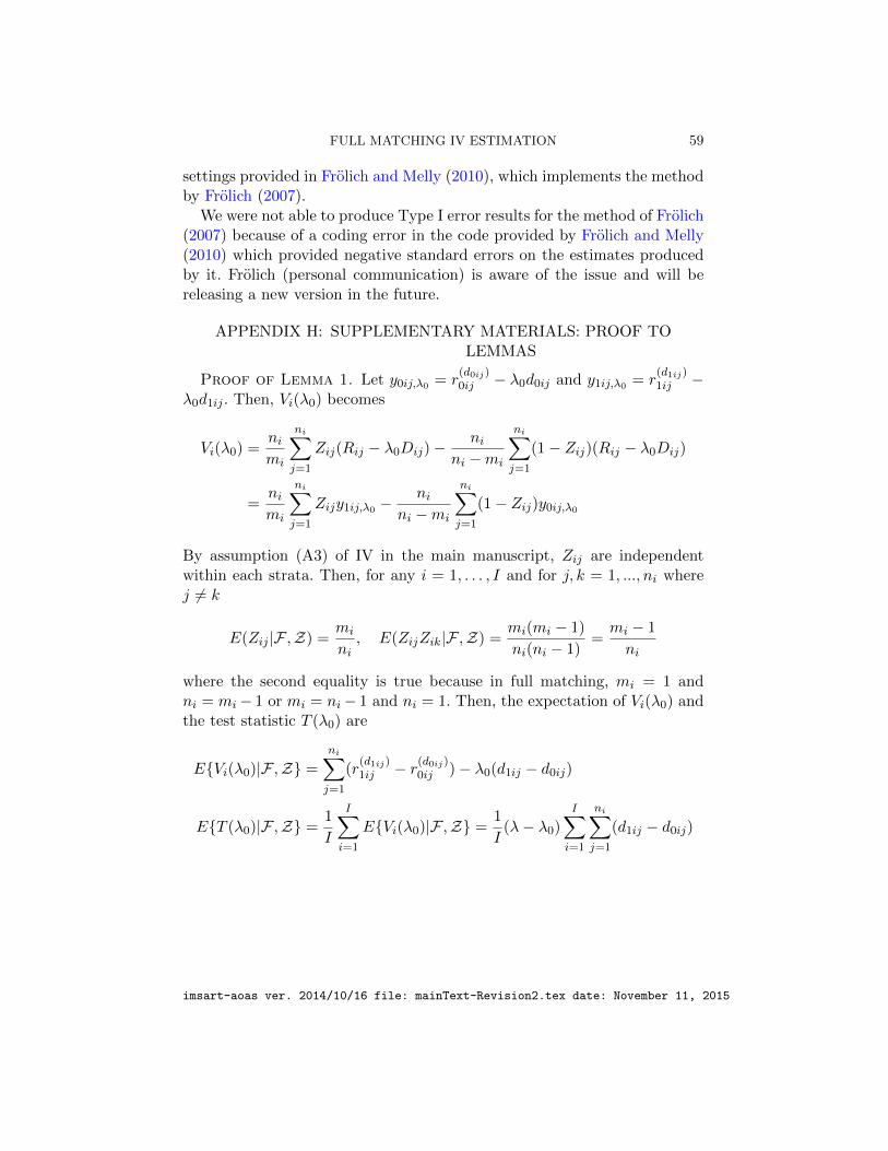
FULL MATCHING IV ESTIMATION 59
settings provided in Frolich and Melly (2010), which implements the methodby Frolich (2007).
We were not able to produce Type I error results for the method of Frolich(2007) because of a coding error in the code provided by Frolich and Melly(2010) which provided negative standard errors on the estimates producedby it. Frolich (personal communication) is aware of the issue and will bereleasing a new version in the future.
APPENDIX H: SUPPLEMENTARY MATERIALS: PROOF TOLEMMAS
Proof of Lemma 1. Let y0ij,λ0 = r(d0ij)0ij − λ0d0ij and y1ij,λ0 = r
(d1ij)1ij −
λ0d1ij . Then, Vi(λ0) becomes
Vi(λ0) =nimi
ni∑j=1
Zij(Rij − λ0Dij)−ni
ni −mi
ni∑j=1
(1− Zij)(Rij − λ0Dij)
=nimi
ni∑j=1
Zijy1ij,λ0 −ni
ni −mi
ni∑j=1
(1− Zij)y0ij,λ0
By assumption (A3) of IV in the main manuscript, Zij are independentwithin each strata. Then, for any i = 1, . . . , I and for j, k = 1, ..., ni wherej 6= k
E(Zij |F ,Z) =mi
ni, E(ZijZik|F ,Z) =
mi(mi − 1)
ni(ni − 1)=mi − 1
ni
where the second equality is true because in full matching, mi = 1 andni = mi− 1 or mi = ni− 1 and ni = 1. Then, the expectation of Vi(λ0) andthe test statistic T (λ0) are
EVi(λ0)|F ,Z =
ni∑j=1
(r(d1ij)1ij − r(d0ij)
0ij )− λ0(d1ij − d0ij)
ET (λ0)|F ,Z =1
I
I∑i=1
EVi(λ0)|F ,Z =1
I(λ− λ0)
I∑i=1
ni∑j=1
(d1ij − d0ij)
imsart-aoas ver. 2014/10/16 file: mainText-Revision2.tex date: November 11, 2015

60 H. KANG ET AL.
For variance of Vi(λ0), Proposition 2 in Rosenbaum (2002, Sec. 2.4.4) givesus
V arVi(λ0)|F ,Z
=V ar
ni∑j=1
Zij
(nimiy1ij,λ0 +
nini −mi
y0ij,λ0
)|F ,Z
=
ni∑j=1
(mi
ni− m2
i
n2i
)a2ij,λ0 +
(mi − 1
ni− m2
i
n2i
)∑j 6=k
aij,λ0aik,λ0
=
(mi
ni− m2
i
n2i
− mi − 1
ni+m2i
n2i
) ni∑j=1
a2ij,λ0 +
(mi − 1
ni− m2
i
n2i
)∑j,k
aij,λ0aik,λ0
=1
ni
ni∑j=1
a2ij,λ0 +
ni(mi − 1)−m2i
n2i
∑j,k
aij,λ0aik,λ0
=1
ni
ni∑j=1
a2ij,λ0 −
1
n2i
∑j,k
aij,λ0aik,λ0
=1
ni
ni∑i=1
(aij,λ0 − ai,λ)2
Finally, the variance of T (λ0) is given by
V arT (λ0)|F ,Z =1
D2
I∑i=1
V arVi(λ0)|F ,Z =1
I2
I∑i=1
1
ni
ni∑j=1
(aij,λ0−ai,λ)2
Proof of Lemma 2. Let v2i,λ0
= V arVi(λ0)|F ,Z. Under the general-
imsart-aoas ver. 2014/10/16 file: mainText-Revision2.tex date: November 11, 2015
FULL MATCHING IV ESTIMATION 61
ized effect ratio, the bias of the estimator (11) is
ES2(λ0)|F ,Z
=1
I(I − 1)
I∑i=1
E[Vi(λ0)− T (λ0)2|F ,Z]
=1
I(I − 1)
I∑i=1
EV 2i (λ0)|F ,Z+ ET 2(λ0)|F ,Z − 2EVi(λ0)T (λ0)|F ,Z
=1
I(I − 1)
I∑i=1
(µ2i,λ0 + vi,λ0) +
µ2λ0 +
1
I2
I∑j=1
vj,λ0
− 2
I
µ2i,λ0 + vi,λ0 +
∑j 6=i
µi,λ0µj,λ0
=
1
I(I − 1)
I∑i=1
vi,λ0 − 2
Ivi,λ0 +
1
I2
I∑j=1
vj,λ0
+
1
I(I − 1)
I∑i=1
µ2i,λ0 + µ2
λ0 −2
I
I∑j=1
µi,λ0µj,λ0
=
(I2 − 2I + I
I(I − 1)
)1
I2
n∑i=1
vi,λ0 +1
I(I − 1)
I∑i=1
(µi,λ0 − µλ0)2
=1
I2
I∑i=1
vi,λ0 +1
I(I − 1)
I∑i=1
(µi,λ0 − µλ0)2
REFERENCES
Serfling, R. (1980). Approximation Theorems of Mathematical Statistics New York: Wiley.Breiman, L. (1992). Probability: Classics in Applied Mathematics, vol. 7, pp. 186, Philadel-
phia: Society for Industrial and Applied Mathematics.Cheng, J. (2011). Using the instrumental propensity score in observational studies for
causal effects. Joint Statistical Meeting Presentation.Frolich, M. (2007). Nonparametric IV estimation of local average treatment effects with
covariates. Journal of Econometrics, 139, 35-75.Frolich, M. and Melly, B. (2010). Estimation of quantile treatment effects with Stata.
Stata Journal, 10, 423-457.Gastwirth, J. L., Krieger, A. M. and Rosenbaum, P. R. (2000). Asymptotic separability
in sensitivity analysis. Journal of the Royal Statistical Society: Series B (StatisticalMethodology), 62, 545-555.
imsart-aoas ver. 2014/10/16 file: mainText-Revision2.tex date: November 11, 2015

62 H. KANG ET AL.
Hansen, B. B. (2004). Full matching in an observational study of coaching for the sat.Journal of the American Statistical Association, 99, 609-618.
Hayfield, T. and Racine, J. (2008). Nonparametric econometrics: the np package Journalof Statistical Software, 27, 1-32.
Hodges, J. L. and Lehmann, E. L. (1963). Estimation of location based on ranks Annalsof Mathematical Statistics, 34, 598-611.
Hogg, R. V., McKean, J. W., and Craig, A. T. (2005). Introduction to MathematicalStatistics, 6th edn. New Jersey: Prentice Hall.
Kang, H., Kreuels, B., Adjei, O., Krumkamp, R., May, J. and Small, D. S. (2013). Thecausal effect of malaria on stunting: a mendelian randomization and matching approach.International Journal of Epidemiology, 42, 1390-1398.
Rosenbaum, P. R. (2002). Observational Studies, 2nd edn. New York: Springer-Verlag.Amplification of sensitivity analysis in matched observational studies. Journal of the
American Statistical Association, 104, 1398-1405.Small, D. S., Gastwirth, J. L., Krieger, A. M., Rosenbaum, P. R. (2009). Simultaneous sen-
sitivity analysis for observational studies using full matching or matching with multiplecontrols Statistics and Its Interface, 2, 203-211.
Wooldridge, J. M. (2010). Econometric Analysis of Cross Section and Panel Data, 2ndedn. Cambridge: MIT Press.
Department of StatisticsThe Wharton SchoolUniversity of PennsylvaniaPhiladelphia, PA, USA19104E-mail: [email protected]
Division of Tropical MedicineI. Department of Internal MedicineUniversity Medical CentreHamburg, Eppendorf, GermanyE-mail: [email protected]
Research Group Infectious Disease EpidemiologyBernhard Nocht Institute for Tropical MedicineHamburg, GermanyE-mail: [email protected]
imsart-aoas ver. 2014/10/16 file: mainText-Revision2.tex date: November 11, 2015