Embed Size (px)
Citation preview
NATURE CHEMISTRY | www.nature.com/naturechemistry 1
SUPPLEMENTARY INFORMATIONDOI: 10.1038/NCHEM.2544
Supplementary Material for “High-resolution mapping of bifurcations in
nonlinear biochemical circuits”
A.J. Genot, A. Baccouche, R. Sieskind, N. Aubert-Kato,
N. Bredeche, J.F. Bartolo, V. Taly, T. Fujii, Y. Rondelez
Contents
S1 Materials and methods 2
S1.1 Sequences and strand design . . . . . . . . . . . . . . . . . . . . . . . . . . . . . . . . . . . . . . . . . 2S1.2 Microfluidic chip . . . . . . . . . . . . . . . . . . . . . . . . . . . . . . . . . . . . . . . . . . . . . . . 3S1.3 Chamber preparation and imaging . . . . . . . . . . . . . . . . . . . . . . . . . . . . . . . . . . . . . 8S1.4 Image processing . . . . . . . . . . . . . . . . . . . . . . . . . . . . . . . . . . . . . . . . . . . . . . . 9S1.5 Content of supplementary files . . . . . . . . . . . . . . . . . . . . . . . . . . . . . . . . . . . . . . . 10
S2 Estimation of barcode di↵usion during droplets generation 11
S3 Scaling of the platform 11
S4 Relative precision of barcoding 12
S5 Thermodynamic analysis of strands in the bistable switch 13
S6 Biochemical orthogonality of dextran barcodes 14
S7 Estimating the 00 zone of the bistable switch 15
S8 Mathematical analysis of the Predator Prey 16
S8.1 Scaling . . . . . . . . . . . . . . . . . . . . . . . . . . . . . . . . . . . . . . . . . . . . . . . . . . . . . 16S8.2 Linear Stability analysis . . . . . . . . . . . . . . . . . . . . . . . . . . . . . . . . . . . . . . . . . . . 17
S9 Computational models for fits 23
S10 Fluorescence images and histograms of the bistable switch 26
S11Droplet array and time traces for the predator-prey system 29
S12 Parasitic reactions 31
S13 Typical concentrations ranges of predators and preys 33
1
High-resolution mapping of bifurcations in nonlinear biochemical circuits
A.J. Genot, A. Baccouche, R. Sieskind, N. Aubert-Kato,
N. Bredeche, J.F. Bartolo, V. Taly, T. Fujii, Y. Rondelez
Contents
S1 Materials and methods 2
S1.1 Sequences and strand design . . . . . . . . . . . . . . . . . . . . . . . . . . . . . . . . . . . . . . . . . 2S1.2 Microfluidic chip . . . . . . . . . . . . . . . . . . . . . . . . . . . . . . . . . . . . . . . . . . . . . . . 3S1.3 Chamber preparation and imaging . . . . . . . . . . . . . . . . . . . . . . . . . . . . . . . . . . . . . 8S1.4 Image processing . . . . . . . . . . . . . . . . . . . . . . . . . . . . . . . . . . . . . . . . . . . . . . . 9S1.5 Content of supplementary files . . . . . . . . . . . . . . . . . . . . . . . . . . . . . . . . . . . . . . . 10
S2 Estimation of barcode di↵usion during droplets generation 11
S3 Scaling of the platform 11
S4 Relative precision of barcoding 12
S5 Thermodynamic analysis of strands in the bistable switch 13
S6 Biochemical orthogonality of dextran barcodes 14
S7 Estimating the 00 zone of the bistable switch 15
S8 Mathematical analysis of the Predator Prey 16
S8.1 Scaling . . . . . . . . . . . . . . . . . . . . . . . . . . . . . . . . . . . . . . . . . . . . . . . . . . . . . 16S8.2 Linear Stability analysis . . . . . . . . . . . . . . . . . . . . . . . . . . . . . . . . . . . . . . . . . . . 17
S9 Computational models for fits 23
S10 Fluorescence images and histograms of the bistable switch 26
S11Droplet array and time traces for the predator-prey system 29
S12 Parasitic reactions 31
S13 Typical concentrations ranges of predators and preys 33
1
© 2016 Macmillan Publishers Limited. All rights reserved.
NATURE CHEMISTRY | www.nature.com/naturechemistry 2
SUPPLEMENTARY INFORMATIONDOI: 10.1038/NCHEM.2544
S1 Materials and methods
S1.1 Sequences and strand design
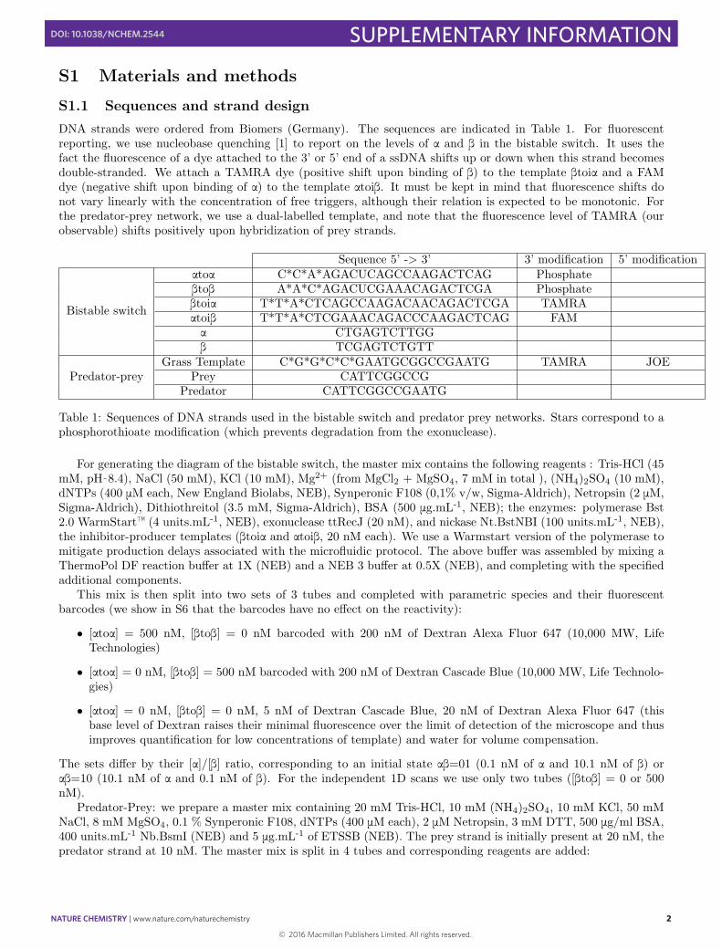
DNA strands were ordered from Biomers (Germany). The sequences are indicated in Table 1. For fluorescentreporting, we use nucleobase quenching [1] to report on the levels of a and b in the bistable switch. It uses thefact the fluorescence of a dye attached to the 3’ or 5’ end of a ssDNA shifts up or down when this strand becomesdouble-stranded. We attach a TAMRA dye (positive shift upon binding of b) to the template btoia and a FAMdye (negative shift upon binding of a) to the template atoib. It must be kept in mind that fluorescence shifts donot vary linearly with the concentration of free triggers, although their relation is expected to be monotonic. Forthe predator-prey network, we use a dual-labelled template, and note that the fluorescence level of TAMRA (ourobservable) shifts positively upon hybridization of prey strands.
Sequence 5’ -> 3’ 3’ modification 5’ modification
Bistable switch
atoa C*C*A*AGACUCAGCCAAGACTCAG Phosphatebtob A*A*C*AGACUCGAAACAGACTCGA Phosphatebtoia T*T*A*CTCAGCCAAGACAACAGACTCGA TAMRAatoib T*T*A*CTCGAAACAGACCCAAGACTCAG FAMa CTGAGTCTTGGb TCGAGTCTGTT
Predator-preyGrass Template C*G*G*C*C*GAATGCGGCCGAATG TAMRA JOE
Prey CATTCGGCCGPredator CATTCGGCCGAATG
Table 1: Sequences of DNA strands used in the bistable switch and predator prey networks. Stars correspond to aphosphorothioate modification (which prevents degradation from the exonuclease).
For generating the diagram of the bistable switch, the master mix contains the following reagents : Tris-HCl (45mM, pH
˜
8.4), NaCl (50 mM), KCl (10 mM), Mg2+ (from MgCl2
+ MgSO4
, 7 mM in total ), (NH4
)2
SO4
(10 mM),dNTPs (400 mM each, New England Biolabs, NEB), Synperonic F108 (0,1% v/w, Sigma-Aldrich), Netropsin (2 mM,Sigma-Aldrich), Dithiothreitol (3.5 mM, Sigma-Aldrich), BSA (500 mg.mL-1, NEB); the enzymes: polymerase Bst2.0 WarmStart™ (4 units.mL-1, NEB), exonuclease ttRecJ (20 nM), and nickase Nt.BstNBI (100 units.mL-1, NEB),the inhibitor-producer templates (btoia and atoib, 20 nM each). We use a Warmstart version of the polymerase tomitigate production delays associated with the microfluidic protocol. The above bu↵er was assembled by mixing aThermoPol DF reaction bu↵er at 1X (NEB) and a NEB 3 bu↵er at 0.5X (NEB), and completing with the specifiedadditional components.
This mix is then split into two sets of 3 tubes and completed with parametric species and their fluorescentbarcodes (we show in S6 that the barcodes have no e↵ect on the reactivity):
• [atoa] = 500 nM, [btob] = 0 nM barcoded with 200 nM of Dextran Alexa Fluor 647 (10,000 MW, LifeTechnologies)
• [atoa] = 0 nM, [btob] = 500 nM barcoded with 200 nM of Dextran Cascade Blue (10,000 MW, Life Technolo-gies)
• [atoa] = 0 nM, [btob] = 0 nM, 5 nM of Dextran Cascade Blue, 20 nM of Dextran Alexa Fluor 647 (thisbase level of Dextran raises their minimal fluorescence over the limit of detection of the microscope and thusimproves quantification for low concentrations of template) and water for volume compensation.
The sets di↵er by their [a]/[b] ratio, corresponding to an initial state ab=01 (0.1 nM of a and 10.1 nM of b) orab=10 (10.1 nM of a and 0.1 nM of b). For the independent 1D scans we use only two tubes ([btob] = 0 or 500nM).
Predator-Prey: we prepare a master mix containing 20 mM Tris-HCl, 10 mM (NH4
)2
SO4
, 10 mM KCl, 50 mMNaCl, 8 mM MgSO
4
, 0.1 % Synperonic F108, dNTPs (400 mM each), 2 mM Netropsin, 3 mM DTT, 500 mg/ml BSA,400 units.mL-1 Nb.BsmI (NEB) and 5 mg.mL-1 of ETSSB (NEB). The prey strand is initially present at 20 nM, thepredator strand at 10 nM. The master mix is split in 4 tubes and corresponding reagents are added:
2
© 2016 Macmillan Publishers Limited. All rights reserved.
NATURE CHEMISTRY | www.nature.com/naturechemistry 3
SUPPLEMENTARY INFORMATIONDOI: 10.1038/NCHEM.2544
• Template: 1.2 mM of template, and 200 nM Dextran Fluorescein (40,000 MW, Anionic, Lysine Fixable, LifeTechnologies)
• Polymerase: 9 % (v/v) of Bst 2.0 WarmStart DNA Polymerase (NEB, stock solution prediluted at 800units.mL-1) with 200 nM of Dextran Alexa Fluor 647
• Exonuclease: 18 % (v/v) of ttRecJ exonuclease (stock solution at 1.53 mM) with 200 nM of Dextran CascadeBlue
• Bu↵er compensation: with 20 nM of Alexa Fluor 647, 5 nM of Dextran Cascade Blue and 20 nM of DextranFITC.
For droplet encapsulation, the surfactant was prepared from a perfluoropolyether carboxy-terminated polymer(Krytox, DuPont) and a polyetheramine (Je↵amine M1000, Huntsmann) based on the synthesis scheme describedin [2]. The continuous phase is a mix of HFE 7500 oil (3M) with 2% (w/w) of surfactant.
S1.2 Microfluidic chip
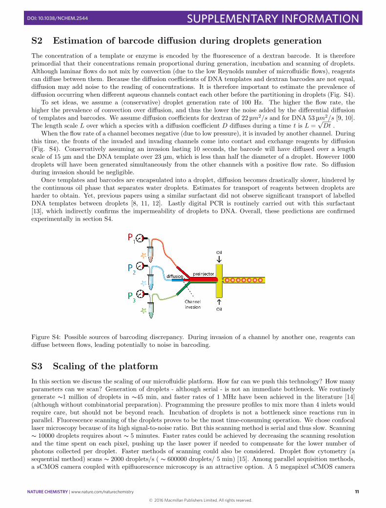
The chip is shown in Fig. S1. The chips were made of PDMS and fabricated by standard soft lithography [3].The mold was fabricated from a chrome mask. The height of the mold (SU-8 2050, MicroChem, USA) is measuredoptically to be 55 mm (+/- 10 mm). The chips were cured at 75ºC for 90 minutes, after which they were peeledo↵, plasma activated and bonded to glass slides. The chips were then baked for 5 hours at 200 ºC to recover theirhydrophobicity and improve bonding [4]. The chip comprises filters, resistances, one oil channel and 4 symmetricaqueous channels. The spacing of the filters was chosen to match that of the constriction (12.5 µm). We insertedresistances in the oil and aqueous channels (prior to the flow-focusing junction) in order to mitigate invasion fromother channels and place the working pressure in the range accessible by our controller (see below). After theconstriction, we added a serpentine channel for accelerating the internal mixing of the droplets and stabilizing thesurfactant layer at the interface [5]. The pre-injector channel upstream of the junction is 300 mm long. Its lengthwas chosen long enough to visualize the co-flow of aqueous channels, and short enough to minimize their contacttime. Droplets are collected from the outlet in a pipette tip.
S1.2.1 Design of resistances
Microfluidic chips can be actuated by two means: flow control or pressure control. In our experiments, we needto rapidly scan a large number of combinations of concentrations, and thus we need a quick actuation. We chosepressure control because it is noticeably faster and more responsive. In an incompressible fluid, pressure jumpspropagate instantly throughout the chip - allowing us to quickly modulate pressures near the junction by varyingthe pressures applied on the inlets. Indeed, for incompressible fluids (div(v) = 0) the pressure field satisfies anequation which does not contain any time-derivative: the pressure Poisson equation. In the laminar regime ofmicrofluidics this equation reduces to the Laplace equation 4P = 0. The pressure is then an harmonic functionwhose value inside the chip is entirely determined by the chip’s boundaries and the pressure applied on inlets andoutlets. By contrast, jumps in flow rate do not propagate immediately -even in incompressible fluids - when channelsare not rigid (which is known to be the case for PDMS and can be worsened by the elastic behaviour of tubing orconnections [6]). Elastic channels act as fluidic capacitors that absorb jumps in flow rates and drastically slow downresponse times. But while pressure control allows for fast actuation, flow rates can become negative (back-flows).Cares need to be taken when programming the pressure profile to ensure that the content of a channel does notinvade significantly another (slight invasion of a channel is still needed to ensure that the corresponding species’concentration sometime reaches 0 nM).
For sake of generality, we consider N aqueous channels (in our chip N = 4). All pressures are defined withrespect to the atmospheric pressure P
o
(pressure at the outlet). We neglect for this model the resistance of thepre-injector, which is short. Let P
i
be the pressure of the aqueous inlet i, Qi
its flow rate and R its hydrodynamicresistance (identical for all aqueous channels). Similarly we define P
oil
, Qoil
and R
oil
the pressure, total flow rateand equivalent resistance of the two oil channels. Let P
junc
be the pressure at the junction, Qout
the flow ratedownstream of the junction and R
out
the corresponding resistance. The pressure of the aqueous channel Pi
and oilchannel P
out
are specified by the user through the pressure controller. On the other hand the flow rates (Qi
, Qout
and Q
oil
) and the junction pressure P
junc
are unknown variables. Those quantities are related linearly by
Q
i
= (Pi
− P
junc
)/R
3
© 2016 Macmillan Publishers Limited. All rights reserved.
NATURE CHEMISTRY | www.nature.com/naturechemistry 4
SUPPLEMENTARY INFORMATIONDOI: 10.1038/NCHEM.2544
Q
oil
= (Poil
− P
junc
)/Roil
Q
out
= (Pjunc
)/Rout
(Note that the viscosities of our HFE oil and water are similar). In order to avoid channel invasion, the flowrates Q
i
must remain positive and thus P
i
= P
junc
(similar conditions also hold for the oil channels). We nowinvestigate the constrains these equations place on the chip. From the conservation of volume for an incompressibleflow, we have
Q
out
=X
i
Q
i
+Q
oil
and thus
(Pjunc
)
R
out
=1
R
X
i
(Pi
− P
junc
) +P
oil
− P
junc
R
oil
we can extract the junction pressure
P
junc
=
Pi
P
i
+ P
oil
R
R
oil
R
R
out
+N + R
R
oil
Note that since the sum of aqueous pressuresP
i
P
i
and the oil pressure P
oil
are kept constant, P
junc
alsoremains constants during droplet generation.
Let us first consider the regime R << R
out,
R
oil
. The junction pressure is then simply the average of thepressures of aqueous inlet
P
junc=
1
N
X
i
P
i
Since it is impossible for all the aqueous pressures to exceed their mean, at least one of the aqueous channelmust be invaded. To avoid this, and provide a reasonable range of available pressures for the scanning process, wedimensionalized the resistances of the oil channels R
oil
and the aqueous channels R to be noticeably larger thanthe resistance of the chip after the junction R
out
(in the current design, Roil
' R and R ' 80Rout
).
4
© 2016 Macmillan Publishers Limited. All rights reserved.
NATURE CHEMISTRY | www.nature.com/naturechemistry 5
SUPPLEMENTARY INFORMATIONDOI: 10.1038/NCHEM.2544
inlet oil
inlet water 1
inlet water 2 inlet water 3
inlet water 4
outlet
w1
w2 w3
w4
oiloil
water
water
Resistance
Filters
Flow-focusing junction
100 µm
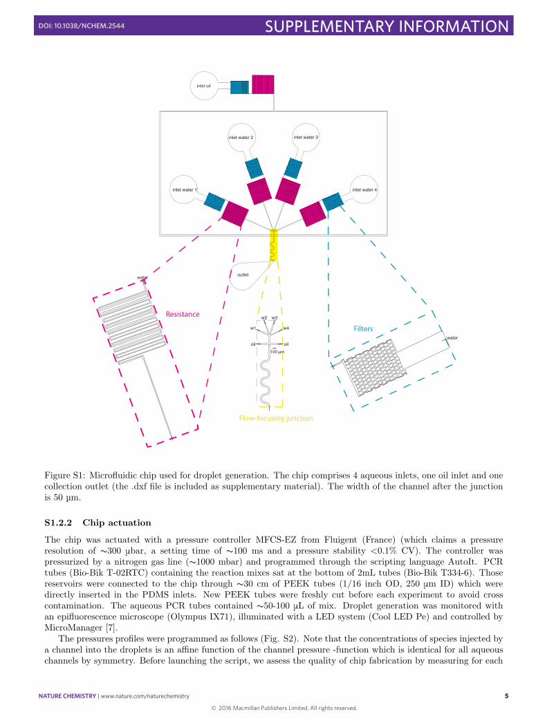
Figure S1: Microfluidic chip used for droplet generation. The chip comprises 4 aqueous inlets, one oil inlet and onecollection outlet (the .dxf file is included as supplementary material). The width of the channel after the junctionis 50 µm.
S1.2.2 Chip actuation
The chip was actuated with a pressure controller MFCS-EZ from Fluigent (France) (which claims a pressureresolution of s300 mbar, a setting time of s100 ms and a pressure stability <0.1% CV). The controller waspressurized by a nitrogen gas line (s1000 mbar) and programmed through the scripting language AutoIt. PCRtubes (Bio-Bik T-02RTC) containing the reaction mixes sat at the bottom of 2mL tubes (Bio-Bik T334-6). Thosereservoirs were connected to the chip through s30 cm of PEEK tubes (1/16 inch OD, 250 mm ID) which weredirectly inserted in the PDMS inlets. New PEEK tubes were freshly cut before each experiment to avoid crosscontamination. The aqueous PCR tubes contained s50-100 mL of mix. Droplet generation was monitored withan epifluorescence microscope (Olympus IX71), illuminated with a LED system (Cool LED Pe) and controlled byMicroManager [7].
The pressures profiles were programmed as follows (Fig. S2). Note that the concentrations of species injected bya channel into the droplets is an affine function of the channel pressure -function which is identical for all aqueouschannels by symmetry. Before launching the script, we assess the quality of chip fabrication by measuring for each
5
© 2016 Macmillan Publishers Limited. All rights reserved.
NATURE CHEMISTRY | www.nature.com/naturechemistry 6
SUPPLEMENTARY INFORMATIONDOI: 10.1038/NCHEM.2544
aqueous channel its minimum pressure Pmin
(the channel is invaded by other channels) and maximum pressure Pmax
(the channel fills the pre-injector and invades other channels) while keeping the total aqueous pressure constant.If the fabrication went well, P
min
and P
max
are similar for all channels. When that is not the case, we discardthe chip. We also add routines for fluorescence calibration which follow the axes atoa= 0nM or btob= 0nM. Thedroplets in the apex of each arms contains 100% of the aqueous mixture of a given channel (Fig. S16 ). The scriptfor each program has been added as Supplementary Information.
2D deterministic exploration (bistable switch, Fig. S2a): The pressure P1
of channel 1 (containing say templateatoa) is quickly cycled from P
min
to P
min
+ (Pmax
− P
min
)/2 in 20 constant steps. Meanwhile, the pressure P
2
ofthe channel 2 (containing the other template btob) is slowly decremented from P
min
+ (Pmax
− P
min
)/2 to P
min
.The pressure P
3
of the compensation channel is adjusted to keep the total aqueous pressure P
1
+ P
2
+ P
3
constantat 600 mbar. The cycle is then repeated, swapping the slow and fast pressures to symmetrize the exploration. Theoil pressure is constant and set to 600 mbar. We repeat the whole process until s30 mL of emulsion is produced(s25 minutes). For 1D scanning, there are only two channels and the pressure of each was simply scanned betweenP
min
and P
max
while keeping their sum constant.3D Monte Carlo sampling (predator-prey oscillator, Fig. S2d): While a deterministic exploration is appropriate
for a 2D space, it becomes prohibitively slow to run and complicated to code in a 3D space. Inspired by statisticalmethods for high-dimensional sampling, we turned to a “Monte-Carlo sampling” to explore the 3D parameter spaceof the predator prey. We generate with Mathematica a random walk in the [0, 1]3 cube which we rescaled (in thescripting software) into [P
min
, P
max
]3 after measuring P
min
and P
max
. We built the random walk by summingthousands of 3D increments (4
1
,42
,43
), where each 4i
is drawn independently from a Pareto distribution (typi-cally with a power of s0.2 and a minimal value of s0.05). Pareto distributions have a long tail which ensures thatthe pressures sometimes “jump” abruptly to new regions of the cube - which is meant to improve coverage. We alsoapply reflections to the random walk so that it remains confined to the cube. The oil pressure is set to 700 mbar.
6
© 2016 Macmillan Publishers Limited. All rights reserved.
NATURE CHEMISTRY | www.nature.com/naturechemistry 7
SUPPLEMENTARY INFORMATIONDOI: 10.1038/NCHEM.2544
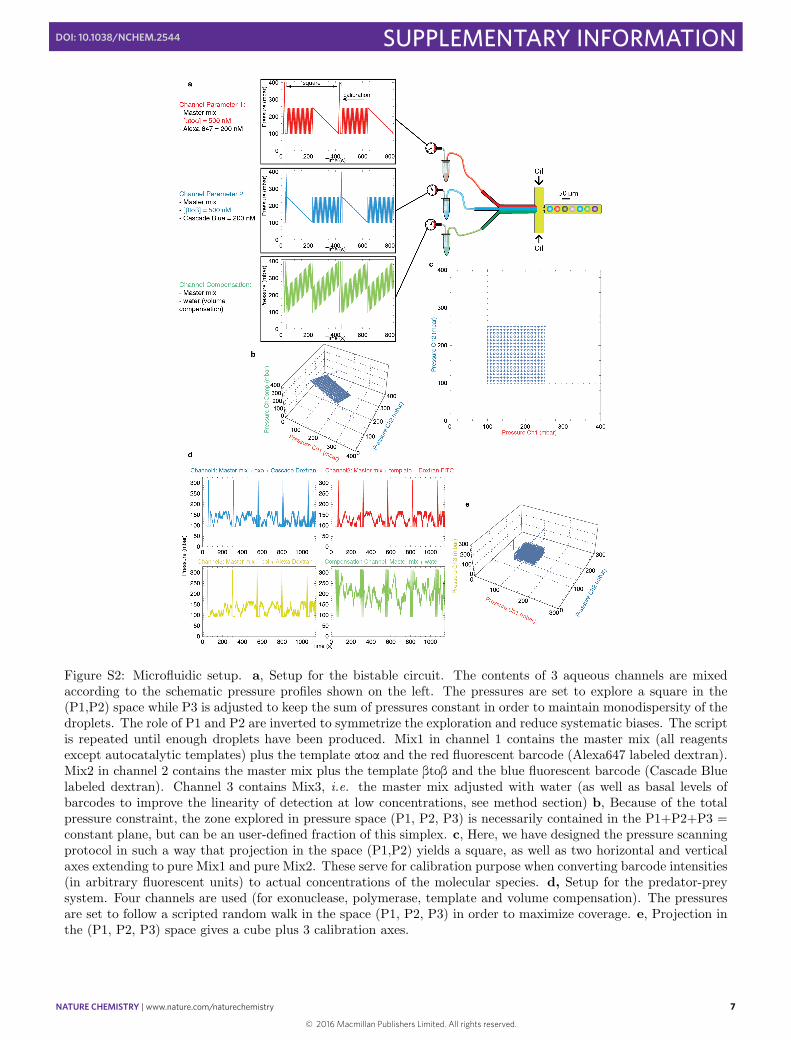
Figure S2: Microfluidic setup. a, Setup for the bistable circuit. The contents of 3 aqueous channels are mixedaccording to the schematic pressure profiles shown on the left. The pressures are set to explore a square in the(P1,P2) space while P3 is adjusted to keep the sum of pressures constant in order to maintain monodispersity of thedroplets. The role of P1 and P2 are inverted to symmetrize the exploration and reduce systematic biases. The scriptis repeated until enough droplets have been produced. Mix1 in channel 1 contains the master mix (all reagentsexcept autocatalytic templates) plus the template atoa and the red fluorescent barcode (Alexa647 labeled dextran).Mix2 in channel 2 contains the master mix plus the template btob and the blue fluorescent barcode (Cascade Bluelabeled dextran). Channel 3 contains Mix3, i.e. the master mix adjusted with water (as well as basal levels ofbarcodes to improve the linearity of detection at low concentrations, see method section) b, Because of the totalpressure constraint, the zone explored in pressure space (P1, P2, P3) is necessarily contained in the P1+P2+P3 =constant plane, but can be an user-defined fraction of this simplex. c, Here, we have designed the pressure scanningprotocol in such a way that projection in the space (P1,P2) yields a square, as well as two horizontal and verticalaxes extending to pure Mix1 and pure Mix2. These serve for calibration purpose when converting barcode intensities(in arbitrary fluorescent units) to actual concentrations of the molecular species. d, Setup for the predator-preysystem. Four channels are used (for exonuclease, polymerase, template and volume compensation). The pressuresare set to follow a scripted random walk in the space (P1, P2, P3) in order to maximize coverage. e, Projection inthe (P1, P2, P3) space gives a cube plus 3 calibration axes.
7
© 2016 Macmillan Publishers Limited. All rights reserved.
NATURE CHEMISTRY | www.nature.com/naturechemistry 8
SUPPLEMENTARY INFORMATIONDOI: 10.1038/NCHEM.2544
S1.3 Chamber preparation and imaging
The droplet emulsion was collected through a tip planted in the outlet. After generation, excess of oil was removedand the emulsion transferred to a 200 mL PCR tube. Droplets were sandwiched between glass slides to form amonolayer. The incubation/observation chamber consisted of a thick glass slide for the bottom (Matsunami Microslide glass 76 mm × 52 mm, thickness s0.8-1.0 mm), and a thin cover slide for the top (Matsunami Micro coverglass 22 mm × 24 mm, thickness s0.12-0.17 mm). Bottom and cover slides were rendered hydrophobic to preventdroplet merging by spin coating a 10% dilution of Cytop CTL-809M (diluted in the provided solvent, Asahi glass)at 500 rpm for 5 seconds then 2000 rpm for 30 seconds. The freshly coated glass slides were then baked at 180ºC for 60 minutes. We used glass beads (Polysciences Inc.) - filtered at 50 mm to match the size of droplets - asspacers to control the thickness of the chamber and prevent the formation of multilayers of droplets. To rigidify thechamber and avoid bending of the thin top slide (which would compromise the spatial homogeneity of the imaging),we poured a photo-curable adhesive (NOA81, Norland Products Inc.) on the spacers. We also added several dropsof NOA on the periphery of the bottom slide. Lastly, to enhance droplet filling and prevent air bubbles, we applieds10 mL of NOA on two parallel edges of the chamber. We then cured the construct with an UV trans illuminatorfor 1 minute. The resulting chamber was filled by capillarity with s25-30 uL of droplet emulsion, closed with NOAand UV cured again (the emulsion was protected from UV exposure by an aluminum foil). Finally, we sealed thechamber with Araldite Rapid (Araldite Professional Adhesives) to improve long-term air tightness.
Droplets were imaged with a confocal laser microscope (Olympus Fluoview FV1000) mounted on a IX-81 chassisand equipped with a xy stage Optosigma Bios-206T, 4 lasers (405, 473, 559 and 635 nm) and a 20x (NA=0.75,bistable switch) or 10x (NA=0.40, predator prey) objective. The droplet chamber was incubated on stage with atransparent heat plate Tokai Hit MAT-1002ROG-KX. Droplets were imaged either at room temperature (bistableswitch, after incubation at 42°C) or at 45°C (predator-prey oscillator, time lapse). The sample was turned upsidedown to reduce the number of glass layers in the optical path, and the total thickness [8]. For time-lapse, the scanningperiod was 6 minutes and the microscope was covered with a black sheet to reduce temperature fluctuations andstray light. After scanning, images were stitched by the Olympus software.
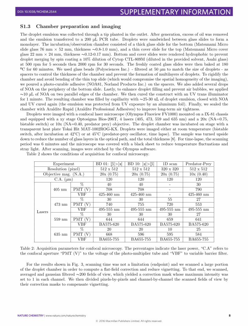
Table 2 shows the conditions of acquisition for confocal microscopy.
Experiment BD 01: [b]>[a] BD 10: [a]>[b] 1D scan Predator-PreyResolution (pixel) 512 x 512 512 x 512 320 x 320 512 x 512
Objective mag. (N.A.) 20x (0.75) 20x (0.75) 20x (0.75) 10x (0.40)C.A. (mm) 120 120 120 120
Lasers
405 nm% 40 40 - 30
PMT (V) 708 708 - 790VBF 425-460 nm 425-460 nm - 425-460 nm
473 nm% 30 30 55 27
PMT (V) 740 755 720 553VBF 495-555 nm 495-555 nm 495-555 nm 495-555 nm
559 nm% 30 30 30 27
PMT (V) 644 644 659 641VBF BA575-620 BA575-620 BA575-620 BA575-620
635 nm% 20 20 10 25
PMT (V) 668 596 595 584VBF BA655-755 BA655-755 BA655-755 BA655-755
Table 2: Acquisition parameters for confocal microscopy. The percentages indicate the laser power, “C.A” refers tothe confocal aperture “PMT (V)” to the voltage of the photo-multiplier tube and “VBF” to variable barrier filter.
For the results shown in Fig. 3, scanning time was not a limitation (endpoint) and we scanned a large portionof the droplet chamber in order to compute a flat-field correction and reduce vignetting. To that end, we scanned,averaged and gaussian filtered s200 fields of view, which yielded a correction mask whose maximum intensity wasset to 1 in each channel. We then divided pixels-by-pixels and channel-by-channel the scanned fields of view bytheir correction masks to compensate vignetting.
8
© 2016 Macmillan Publishers Limited. All rights reserved.
NATURE CHEMISTRY | www.nature.com/naturechemistry 9
SUPPLEMENTARY INFORMATIONDOI: 10.1038/NCHEM.2544
S1.4 Image processing
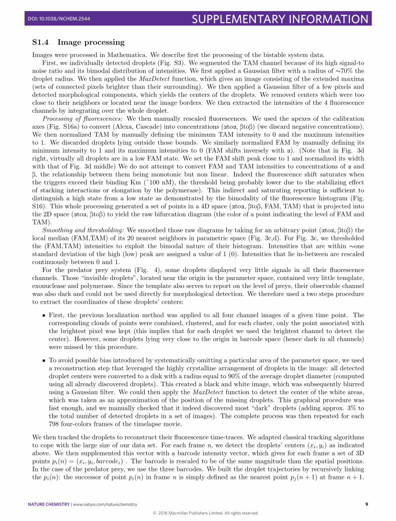
Images were processed in Mathematica. We describe first the processing of the bistable system data.First, we individually detected droplets (Fig. S3). We segmented the TAM channel because of its high signal-to
noise ratio and its bimodal distribution of intensities. We first applied a Gaussian filter with a radius of s70% thedroplet radius. We then applied the MaxDetect function, which gives an image consisting of the extended maxima(sets of connected pixels brighter than their surrounding). We then applied a Gaussian filter of a few pixels anddetected morphological components, which yields the centers of the droplets. We removed centers which were tooclose to their neighbors or located near the image borders. We then extracted the intensities of the 4 fluorescencechannels by integrating over the whole droplet.
Processing of fluorescences: We then manually rescaled fluorescences. We used the apexes of the calibrationaxes (Fig. S16a) to convert (Alexa, Cascade) into concentrations (atoa, btob) (we discard negative concentrations).We then normalized TAM by manually defining the minimum TAM intensity to 0 and the maximum intensitiesto 1. We discarded droplets lying outside those bounds. We similarly normalized FAM by manually defining itsminimum intensity to 1 and its maximum intensities to 0 (FAM shifts inversely with a). (Note that in Fig. 3dright, virtually all droplets are in a low FAM state. We set the FAM shift peak close to 1 and normalized its widthwith that of Fig. 3d middle) We do not attempt to convert FAM and TAM intensities to concentrations of a andb, the relationship between them being monotonic but non linear. Indeed the fluorescence shift saturates whenthe triggers exceed their binding Km (˜100 nM), the threshold being probably lower due to the stabilizing e↵ectof stacking interactions or elongation by the polymerase). This indirect and saturating reporting is sufficient todistinguish a high state from a low state as demonstrated by the bimodality of the fluorescence histogram (Fig.S16). This whole processing generated a set of points in a 4D space (atoa, btob, FAM, TAM) that is projected intothe 2D space (atoa, btob) to yield the raw bifurcation diagram (the color of a point indicating the level of FAM andTAM).
Smoothing and thresholding: We smoothed those raw diagrams by taking for an arbitrary point (atoa, btob) thelocal median (FAM,TAM) of its 20 nearest neighbors in parametric space (Fig. 3c,d). For Fig. 3c, we thresholdedthe (FAM,TAM) intensities to exploit the bimodal nature of their histogram. Intensities that are within sonestandard deviation of the high (low) peak are assigned a value of 1 (0). Intensities that lie in-between are rescaledcontinuously between 0 and 1.
For the predator prey system (Fig. 4), some droplets displayed very little signals in all their fluorescencechannels. Those “invisible droplets”, located near the origin in the parameter space, contained very little template,exonuclease and polymerase. Since the template also serves to report on the level of preys, their observable channelwas also dark and could not be used directly for morphological detection. We therefore used a two steps procedureto extract the coordinates of these droplets’ centers:
• First, the previous localization method was applied to all four channel images of a given time point. Thecorresponding clouds of points were combined, clustered, and for each cluster, only the point associated withthe brightest pixel was kept (this implies that for each droplet we used the brightest channel to detect thecenter). However, some droplets lying very close to the origin in barcode space (hence dark in all channels)were missed by this procedure.
• To avoid possible bias introduced by systematically omitting a particular area of the parameter space, we useda reconstruction step that leveraged the highly crystalline arrangement of droplets in the image: all detecteddroplet centers were converted to a disk with a radius equal to 90% of the average droplet diameter (computedusing all already discovered droplets). This created a black and white image, which was subsequently blurredusing a Gaussian filter. We could then apply the MaxDetect function to detect the center of the white areas,which was taken as an approximation of the position of the missing droplets. This graphical procedure wasfast enough, and we manually checked that it indeed discovered most “dark” droplets (adding approx. 3% tothe total number of detected droplets in a set of images). The complete process was then repeated for each798 four-colors frames of the timelapse movie.
We then tracked the droplets to reconstruct their fluorescence time-traces. We adapted classical tracking algorithmsto cope with the large size of our data set. For each frame n, we detect the droplets’ centers (x
i
, y
i
) as indicatedabove. We then supplemented this vector with a barcode intensity vector, which gives for each frame a set of 3Dpoints p
i
(n) = (xi
, y
i
, barcode
i
) . The barcode is rescaled to be of the same magnitude than the spatial positions.In the case of the predator prey, we use the three barcodes. We built the droplet trajectories by recursively linkingthe p
i
(n): the successor of point pi
(n) in frame n is simply defined as the nearest point pj
(n + 1) at frame n + 1.
9
© 2016 Macmillan Publishers Limited. All rights reserved.
NATURE CHEMISTRY | www.nature.com/naturechemistry 10
SUPPLEMENTARY INFORMATIONDOI: 10.1038/NCHEM.2544
In other words we do not attempt to minimize the total deviation of centers between frames, which allows trackingto be parallelized and significantly sped up. This choice is justified by the fact that droplets move very little, andthat the barcode dimension further decreases tracking errors. We then remove trajectories with large jumps andverify on randomly selected droplets the correctness of tracking.
Once we had a trajectory associated to each droplet, we could extract the fluorescence time trace by takingdroplet-averaged fluorescence values as above. These time traces were smoothed (moving average over 8 frames)and detrended using the built-in Mathematica functions. Peak positions and heights were then detected using theFindPeak function and used directly to compute the oscillation score.
Figure S3: Extracting the centers of droplets. The raw image is first smoothed with a gaussian filter. Localfluorescence maxima (roughly a small rectangle located around the brightest point of each droplets) are thendetected and smoothed slightly (note that the local maxima are enlarged for sake of clarity in this figure). Theresulting image is then segmented to provide morphological components, centroids of which are used as centers ofdroplets.
S1.5 Content of supplementary files
• Droplet array for the bistable switch (Alexa channel): This image shows the fluorescence in the Alexachannel of an array of droplets generated for the experiment on the bistable switch. It corresponds to theimage in section section S10 of this Supplementary Material.
• Droplet array for the bistable switch (Cascade channel): This image shows the fluorescence in theCascade channel of an array of droplets generated for the experiment on the bistable switch.
• Droplet array for the bistable switch (FAM channel): This image shows the fluorescence in the FAMchannel of an array of droplets generated for the experiment on the bistable switch.
• Droplet array for the bistable switch (TAMRA channel): This image shows the fluorescence in theTAMRA channel of an array of droplets generated for the experiment on the bistable switch.
• Chip design: This CAD file contains the Autocad source for the chip design.
• Movie 1: This movie shows the scanning of inlet pressures near the microfluidic junction. Channels containfluorescence dyes for visualization. Note that the script has been slowed down to facilitate recording.
• Movie 2: This time-lapse movie shows the fluorescence of droplets in the TAMRA channel. The variable tdenotes the frame number.
• Movie 3: Example of sustained and bursting oscillations.
• Pressure script used for Bistable switch: This Autoit file contains the script used for generating thepressure profiles in the bistable switch experiment
• Pressure script used for predator prey: This Autoit file contains the script used for generating thepressure profiles in the Predator Prey experiment.
10
© 2016 Macmillan Publishers Limited. All rights reserved.
NATURE CHEMISTRY | www.nature.com/naturechemistry 11
SUPPLEMENTARY INFORMATIONDOI: 10.1038/NCHEM.2544
S2 Estimation of barcode di↵usion during droplets generation
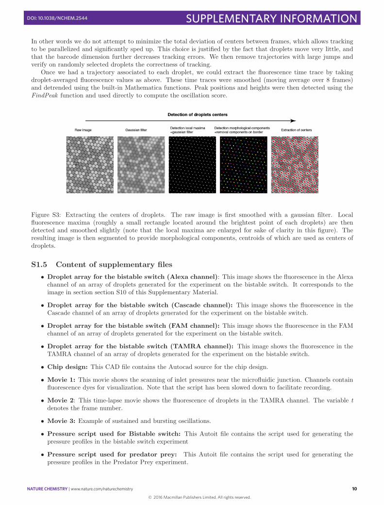
The concentration of a template or enzyme is encoded by the fluorescence of a dextran barcode. It is thereforeprimordial that their concentrations remain proportional during generation, incubation and scanning of droplets.Although laminar flows do not mix by convection (due to the low Reynolds number of microfluidic flows), reagentscan di↵use between them. Because the di↵usion coefficients of DNA templates and dextran barcodes are not equal,di↵usion may add noise to the reading of concentrations. It is therefore important to estimate the prevalence ofdi↵usion occurring when di↵erent aqueous channels contact each other before the partitioning in droplets (Fig. S4).
To set ideas, we assume a (conservative) droplet generation rate of 100 Hz. The higher the flow rate, thehigher the prevalence of convection over di↵usion, and thus the lower the noise added by the di↵erential di↵usionof templates and barcodes. We assume di↵usion coefficients for dextran of 22µm2
/s and for DNA 53µm2
/s [9, 10].The length scale L over which a species with a di↵usion coefficient D di↵uses during a time t is L =
pDt .
When the flow rate of a channel becomes negative (due to low pressure), it is invaded by another channel. Duringthis time, the fronts of the invaded and invading channels come into contact and exchange reagents by di↵usion(Fig. S4). Conservatively assuming an invasion lasting 10 seconds, the barcode will have di↵used over a lengthscale of 15 mm and the DNA template over 23 mm, which is less than half the diameter of a droplet. However 1000droplets will have been generated simultaneously from the other channels with a positive flow rate. So di↵usionduring invasion should be negligible.
Once templates and barcodes are encapsulated into a droplet, di↵usion becomes drastically slower, hindered bythe continuous oil phase that separates water droplets. Estimates for transport of reagents between droplets areharder to obtain. Yet, previous papers using a similar surfactant did not observe significant transport of labelledDNA templates between droplets [8, 11, 12]. Lastly digital PCR is routinely carried out with this surfactant[13], which indirectly confirms the impermeability of droplets to DNA. Overall, these predictions are confirmedexperimentally in section S4.
Figure S4: Possible sources of barcoding discrepancy. During invasion of a channel by another one, reagents candi↵use between flows, leading potentially to noise in barcoding.
S3 Scaling of the platform
In this section we discuss the scaling of our microfluidic platform. How far can we push this technology? How manyparameters can we scan? Generation of droplets - although serial - is not an immediate bottleneck. We routinelygenerate s1 million of droplets in s45 min, and faster rates of 1 MHz have been achieved in the literature [14](although without combinatorial preparation). Programming the pressure profiles to mix more than 4 inlets wouldrequire care, but should not be beyond reach. Incubation of droplets is not a bottleneck since reactions run inparallel. Fluorescence scanning of the droplets proves to be the most time-consuming operation. We chose confocallaser microscopy because of its high signal-to-noise ratio. But this scanning method is serial and thus slow. Scannings 10000 droplets requires about s 5 minutes. Faster rates could be achieved by decreasing the scanning resolutionand the time spent on each pixel, pushing up the laser power if needed to compensate for the lower number ofphotons collected per droplet. Faster methods of scanning could also be considered. Droplet flow cytometry (asequential method) scans s 2000 droplets/s ( s 600000 droplets/ 5 min) [15]. Among parallel acquisition methods,a sCMOS camera coupled with epifluorescence microscopy is an attractive option. A 5 megapixel sCMOS camera
11
© 2016 Macmillan Publishers Limited. All rights reserved.
NATURE CHEMISTRY | www.nature.com/naturechemistry 12
SUPPLEMENTARY INFORMATIONDOI: 10.1038/NCHEM.2544
can nominally scan s 50000 droplets simultaneously at a resolution of 100 pixels/droplet. Assuming an acquisitiontime on the order of 10 seconds per frame (including stage translation, filter switching and exposure), a sCMOSsetup will record the fluorescence of 1.5 million droplets per 5 minutes. Note that parallel scanning methods requiremore careful calibration than sequential ones to account for the spatial dependence of the illumination and sensors.Fluorescence overlap will also have to be dealt with, but it is realistic to encode the concentration of 6 variablessimultaneously [16]. For example in the case of the bistable switch, this would give 4 parameters (two autocatalytictemplates and two initial concentrations of triggers) and two observables (steady state level of triggers), thusproviding in a single experiment not only the complete 2-dimensional bifurcation diagram, but also the basins ofattraction corresponding to each parameter set.
S4 Relative precision of barcoding
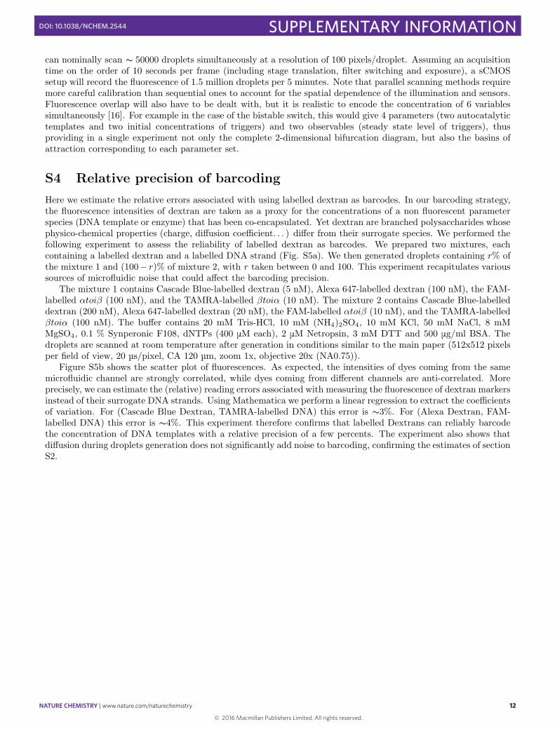
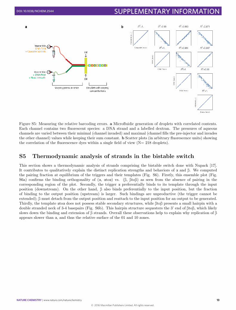
Here we estimate the relative errors associated with using labelled dextran as barcodes. In our barcoding strategy,the fluorescence intensities of dextran are taken as a proxy for the concentrations of a non fluorescent parameterspecies (DNA template or enzyme) that has been co-encapsulated. Yet dextran are branched polysaccharides whosephysico-chemical properties (charge, di↵usion coefficient. . . ) di↵er from their surrogate species. We performed thefollowing experiment to assess the reliability of labelled dextran as barcodes. We prepared two mixtures, eachcontaining a labelled dextran and a labelled DNA strand (Fig. S5a). We then generated droplets containing r% ofthe mixture 1 and (100− r)% of mixture 2, with r taken between 0 and 100. This experiment recapitulates varioussources of microfluidic noise that could a↵ect the barcoding precision.
The mixture 1 contains Cascade Blue-labelled dextran (5 nM), Alexa 647-labelled dextran (100 nM), the FAM-labelled ↵toiβ (100 nM), and the TAMRA-labelled βtoi↵ (10 nM). The mixture 2 contains Cascade Blue-labelleddextran (200 nM), Alexa 647-labelled dextran (20 nM), the FAM-labelled ↵toiβ (10 nM), and the TAMRA-labelledβtoi↵ (100 nM). The bu↵er contains 20 mM Tris-HCl, 10 mM (NH
4
)2
SO4
, 10 mM KCl, 50 mM NaCl, 8 mMMgSO
4
, 0.1 % Synperonic F108, dNTPs (400 mM each), 2 mM Netropsin, 3 mM DTT and 500 mg/ml BSA. Thedroplets are scanned at room temperature after generation in conditions similar to the main paper (512x512 pixelsper field of view, 20 µs/pixel, CA 120 µm, zoom 1x, objective 20x (NA0.75)).
Figure S5b shows the scatter plot of fluorescences. As expected, the intensities of dyes coming from the samemicrofluidic channel are strongly correlated, while dyes coming from di↵erent channels are anti-correlated. Moreprecisely, we can estimate the (relative) reading errors associated with measuring the fluorescence of dextran markersinstead of their surrogate DNA strands. Using Mathematica we perform a linear regression to extract the coefficientsof variation. For (Cascade Blue Dextran, TAMRA-labelled DNA) this error is s3%. For (Alexa Dextran, FAM-labelled DNA) this error is s4%. This experiment therefore confirms that labelled Dextrans can reliably barcodethe concentration of DNA templates with a relative precision of a few percents. The experiment also shows thatdi↵usion during droplets generation does not significantly add noise to barcoding, confirming the estimates of sectionS2.
12
© 2016 Macmillan Publishers Limited. All rights reserved.
NATURE CHEMISTRY | www.nature.com/naturechemistry 13
SUPPLEMENTARY INFORMATIONDOI: 10.1038/NCHEM.2544
Figure S5: Measuring the relative barcoding errors. a Microfluidic generation of droplets with correlated contents.Each channel contains two fluorescent species: a DNA strand and a labelled dextran. The pressures of aqueouschannels are varied between their minimal (channel invaded) and maximal (channel fills the pre-injector and invadesthe other channel) values while keeping their sum constant. b Scatter plots (in arbitrary fluorescence units) showingthe correlation of the fluorescence dyes within a single field of view (N= 218 droplets).
S5 Thermodynamic analysis of strands in the bistable switch
This section shows a thermodynamic analysis of strands comprising the bistable switch done with Nupack [17].It contributes to qualitatively explain the distinct replication strengths and behaviors of a and b. We computedthe pairing fraction at equilibrium of the triggers and their templates (Fig. S6). Firstly, this ensemble plot (Fig.S6a) confirms the binding orthogonality of (a, atoa) vs. (b, btob) as seen from the absence of pairing in thecorresponding region of the plot. Secondly, the trigger a preferentially binds to its template through the inputposition (downstream). On the other hand, b also binds preferentially to the input position, but the fractionof binding to the output position (upstream) is larger. Such bindings are unproductive (the trigger cannot beextended); b must detach from the output position and reattach to the input position for an output to be generated.Thirdly, the template atoa does not possess stable secondary structures, while btob presents a small hairpin with adouble stranded neck of 3-4 basepairs (Fig. S6b). This hairpin structure sequesters the 3’ end of btob, which likelyslows down the binding and extension of b strands. Overall these observations help to explain why replication of bappears slower than a, and thus the relative surface of the 01 and 10 zones.
13
© 2016 Macmillan Publishers Limited. All rights reserved.

NATURE CHEMISTRY | www.nature.com/naturechemistry 14
SUPPLEMENTARY INFORMATIONDOI: 10.1038/NCHEM.2544
αtoα
βtoβ β/βtoβ
α/αtoαba
Figure S6: Thermodynamic analysis of the bistable switch. a Ensemble pair plot for a mixture of atoa (200 nM),btob (200 nM), a (50 nM) and b (50 nM). We use the following conditions: 42°C, 8 mM Mg
2+and 50 mM Na
+.Because Nupack cannot handle hybrid RNA/DNA polymer, U bases were replaced by T bases. b Minimum FreeEnergy structure for each complex.
S6 Biochemical orthogonality of dextran barcodes
To investigate the possible e↵ects of labelled dextrans on the reactivity of the PEN DNA toolbox, we mon-itored a predator-prey system with increasing concentrations of dextran labelled with Alexa 647 or CascadeBlue (experiment performed in a CFX Real-Time PCR System thermocycler). We mix the grass template (5’C*G*G*CCGAATGCGGCCGAATG-dy530 3’, 140 nM), the prey strand (5’ CATTCGGCCG 3’, 20 nM) and thepredator strand (5’ CATTCGGCCGAATG 3’, 10 nM) in a bu↵er containing 20 mM Tris-HCl, 10 mM (NH
4
)2
SO4
,10 mM KCl, 50 mM NaCl, 8 mM MgSO
4
, 0.1 % Synperonic F108 , 400 mM of each dNTP , 2 mM Netropsin , 1 eq.EvaGreen, 3 mM DTT, 500 mg/ml BSA and 5 mg/ml of ETSSB, 50 units.mL-1 Bst DNA Polymerase Full Length(NEB), 20 nM of ttRecJ exonuclease, 400 units.mL-1 Nb.BsmI, and 0 nM to 1 mM of each labelled dextran.
14
© 2016 Macmillan Publishers Limited. All rights reserved.
NATURE CHEMISTRY | www.nature.com/naturechemistry 15
SUPPLEMENTARY INFORMATIONDOI: 10.1038/NCHEM.2544
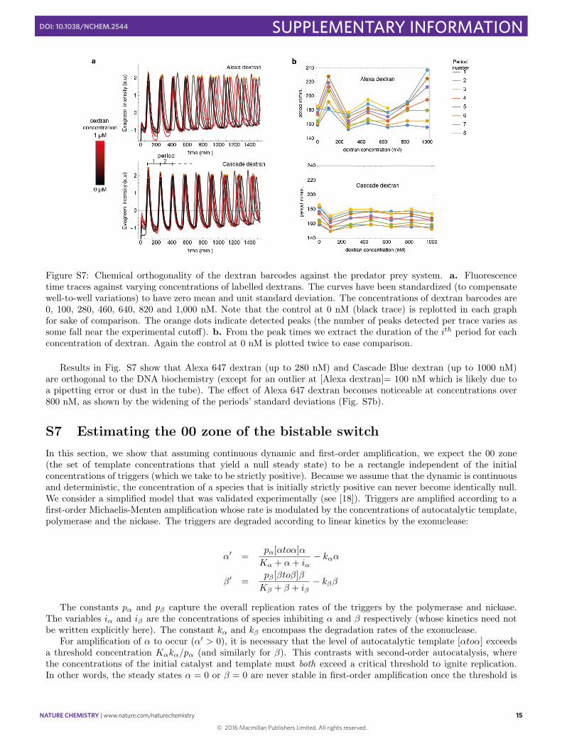
Figure S7: Chemical orthogonality of the dextran barcodes against the predator prey system. a. Fluorescencetime traces against varying concentrations of labelled dextrans. The curves have been standardized (to compensatewell-to-well variations) to have zero mean and unit standard deviation. The concentrations of dextran barcodes are0, 100, 280, 460, 640, 820 and 1,000 nM. Note that the control at 0 nM (black trace) is replotted in each graphfor sake of comparison. The orange dots indicate detected peaks (the number of peaks detected per trace varies assome fall near the experimental cuto↵). b. From the peak times we extract the duration of the i
th period for eachconcentration of dextran. Again the control at 0 nM is plotted twice to ease comparison.
Results in Fig. S7 show that Alexa 647 dextran (up to 280 nM) and Cascade Blue dextran (up to 1000 nM)are orthogonal to the DNA biochemistry (except for an outlier at [Alexa dextran]= 100 nM which is likely due toa pipetting error or dust in the tube). The e↵ect of Alexa 647 dextran becomes noticeable at concentrations over800 nM, as shown by the widening of the periods’ standard deviations (Fig. S7b).
S7 Estimating the 00 zone of the bistable switch
In this section, we show that assuming continuous dynamic and first-order amplification, we expect the 00 zone(the set of template concentrations that yield a null steady state) to be a rectangle independent of the initialconcentrations of triggers (which we take to be strictly positive). Because we assume that the dynamic is continuousand deterministic, the concentration of a species that is initially strictly positive can never become identically null.We consider a simplified model that was validated experimentally (see [18]). Triggers are amplified according to afirst-order Michaelis-Menten amplification whose rate is modulated by the concentrations of autocatalytic template,polymerase and the nickase. The triggers are degraded according to linear kinetics by the exonuclease:
↵
0 =p
↵
[↵to↵]↵
K
↵
+ ↵+ i
↵
− k
↵
↵
β
0 =p
β
[βtoβ]β
K
β
+ β + i
β
− k
β
β
The constants p
↵
and p
β
capture the overall replication rates of the triggers by the polymerase and nickase.The variables i
↵
and i
β
are the concentrations of species inhibiting ↵ and β respectively (whose kinetics need notbe written explicitly here). The constant k
↵
and k
β
encompass the degradation rates of the exonuclease.For amplification of ↵ to occur (↵0
> 0), it is necessary that the level of autocatalytic template [↵to↵] exceedsa threshold concentration K
↵
k
↵
/p
↵
(and similarly for β). This contrasts with second-order autocatalysis, wherethe concentrations of the initial catalyst and template must both exceed a critical threshold to ignite replication.In other words, the steady states ↵ = 0 or β = 0 are never stable in first-order amplification once the threshold is
15
© 2016 Macmillan Publishers Limited. All rights reserved.
NATURE CHEMISTRY | www.nature.com/naturechemistry 16
SUPPLEMENTARY INFORMATIONDOI: 10.1038/NCHEM.2544
crossed because any infinisitimal level of trigger will be amplified. Let us define the rectangle R
00
in the parameterspace (↵to↵, βtoβ) by
R
00
= {0 ↵to↵ K
↵
k
↵
/p
↵
, 0 βtoβ K
β
k
β
/p
β
}This rectangle is thus necessarily included in the 00 zone. Now we prove the reverse inclusion, namely that the
00 zone is included in the rectangle. Suppose that we start outside R
00
(at least one template exceeds its thresholdlevel) but that ↵ and β both asymptotically decay to zero. Then the inhibitors also eventually decay to zero. Aftera (possibly long) relaxation time T1, we have β, i
β
⌧ K
β
and ↵, i
↵
⌧ K
↵
and thus
↵
0 = (p
↵
[↵to↵]
K
↵
− k
↵
)↵
β
0 = (p
β
[βtoβ]
K
β
− k
β
)β
Given ↵ and β are both non null (because of to their deterministic and continuous evolution), at least one speciesis amplifying (the species whose template exceeds its threshold concentration), which contradicts the assumptionsthat the system is converging toward the null state.
This simple model predicts that the 00 zone should be a rectangle whose shape is independent of the initialconcentrations of triggers. Since this is clearly not the case in Figure 3, at least one of our hypothesis must be false.Firstly, the actual mechanism of replication may be higher-order, which would provide the necessary hysteresis tostabilize the steady state ↵ = 0 or β = 0. Secondly, the dynamic may not be fully continuous. The concentrationsof a and b cannot be arbitrarily low without being null (40 fM × 65 pL ⇡ 1 molecule). In their race againstdegradation, the autocatalytic templates may sometime lose and the copy numbers of a and b both reach andremain at 0 (something impossible in a well-posed, deterministic ODE because of the uniqueness of its solution).Since a template cannot replicate a strand that is absent, the 00 zone in our diagram may therefore represent circuitsthat are “stochastically trapped” in the null state 00. Lastly, when the levels of templates are close (but superior)to their thresholds, the relaxation may drastically slow down and exceed our experimental time scale (10 hours).This phenomenon would be reminiscent of critical slowdown, where some dynamic systems have been shown to takea very long time to recover from quasi-lethal perturbations [19].
S8 Mathematical analysis of the Predator Prey
S8.1 Scaling
Here we show from scaling arguments that the quantity µ = exo
tem⇥pol
plays a role in shaping the oscillatory region
of the predator-prey system (Fig. 4 in the main paper). We consider a general kinetic model with 3 biochemicalreactions of replication, predation and decay. For sake of generality, we do not assume much about their innerkinetics, except than their rates vary linearly with their catalysts concentrations. This encompasses most enzymaticmodels such as Michaelis-Menten, Hill cooperativity or competitive inhibition. We model the dynamics of preysand predators (noted x(t) and y(t) respectively) as follows:
dx(t)
dt
= tem · pol · f(x, y)− pol · g(x, y)− exo · h(x, y)
dy(t)
dt
= pol · g(x, y)− exo · l(x, y)
The term f(x, y) represents the replication of preys, mediated by the polymerase and the template. The secondterm g(x, y) represents the predation reaction, mediated only by the polymerase. The last terms h(x, y) and l(x, y)represent the degradation of preys or predators by the exonuclease. Factorizing the equations by tem⇥ pol, we get:
dx(t)
dt
= tem · pol(f(x, y)− 1
tem
g(x, y)− exo
tem⇥ pol
· h(x, y))
dy(t)
dt
= tem · pol( 1
tem
g(x, y)− exo
tem · pol · l(x, y))
16
© 2016 Macmillan Publishers Limited. All rights reserved.
NATURE CHEMISTRY | www.nature.com/naturechemistry 17
SUPPLEMENTARY INFORMATIONDOI: 10.1038/NCHEM.2544
Now we define the reduced constants µ = exo
tem·pol and ⌘ = 1/tem. We also define a time-rescaled variable x
0 by
x
0(t) = x( t
tem·pol ) (and similarly for y and y
0). We obtain the reduced system:
dx
0(t)
dt
= f(x0, y
0)− ⌘g(x0, y
0)− µh(x0, y
0))
dy
0(t)
dt
= ⌘g(x0, y
0)− µl(x0, y
0)
This reduction shows that the dynamics of droplets with identical µ and ⌘ will be identical modulo an individualrescaling of time. In other words, droplets with identical (µ,⌘) in the oscillatory region will oscillate with a periodproportional to 1
tem·pol .
S8.2 Linear Stability analysis
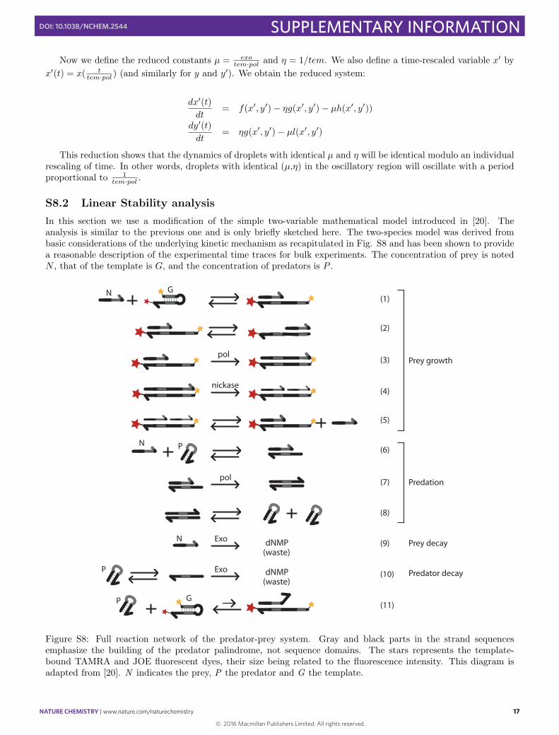
In this section we use a modification of the simple two-variable mathematical model introduced in [20]. Theanalysis is similar to the previous one and is only briefly sketched here. The two-species model was derived frombasic considerations of the underlying kinetic mechanism as recapitulated in Fig. S8 and has been shown to providea reasonable description of the experimental time traces for bulk experiments. The concentration of prey is notedN , that of the template is G, and the concentration of predators is P .
dNMP (waste)
dNMP (waste)
pol
nickase
pol
Exo
Exo
(1)
(2)
(3)
(4)
(5)
(6)
(7)
(8)
(9)
(10)
N G
Prey growth
Predation
Prey decay
Predator decay
N P
N
P
G(11)P
Figure S8: Full reaction network of the predator-prey system. Gray and black parts in the strand sequencesemphasize the building of the predator palindrome, not sequence domains. The stars represents the template-bound TAMRA and JOE fluorescent dyes, their size being related to the fluorescence intensity. This diagram isadapted from [20]. N indicates the prey, P the predator and G the template.
17
© 2016 Macmillan Publishers Limited. All rights reserved.
NATURE CHEMISTRY | www.nature.com/naturechemistry 18
SUPPLEMENTARY INFORMATIONDOI: 10.1038/NCHEM.2544
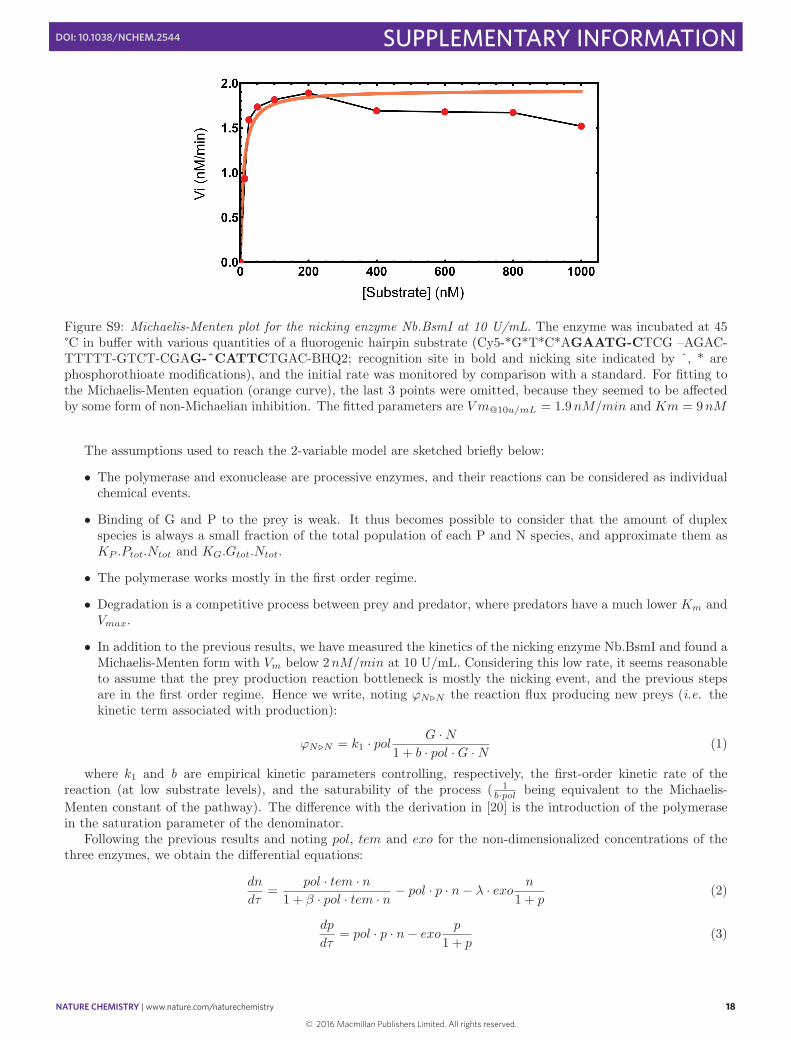
Figure S9: Michaelis-Menten plot for the nicking enzyme Nb.BsmI at 10 U/mL. The enzyme was incubated at 45°C in bu↵er with various quantities of a fluorogenic hairpin substrate (Cy5-*G*T*C*AGAATG-CTCG –AGAC-TTTTT-GTCT-CGAG-ˆCATTCTGAC-BHQ2; recognition site in bold and nicking site indicated by ˆ, * arephosphorothioate modifications), and the initial rate was monitored by comparison with a standard. For fitting tothe Michaelis-Menten equation (orange curve), the last 3 points were omitted, because they seemed to be a↵ectedby some form of non-Michaelian inhibition. The fitted parameters are V m
@10u/mL
= 1.9nM/min and Km = 9nM
The assumptions used to reach the 2-variable model are sketched briefly below:
• The polymerase and exonuclease are processive enzymes, and their reactions can be considered as individualchemical events.
• Binding of G and P to the prey is weak. It thus becomes possible to consider that the amount of duplexspecies is always a small fraction of the total population of each P and N species, and approximate them asK
P
.P
tot
.N
tot
and K
G
.G
tot
.N
tot
.
• The polymerase works mostly in the first order regime.
• Degradation is a competitive process between prey and predator, where predators have a much lower Km
andV
max
.
• In addition to the previous results, we have measured the kinetics of the nicking enzyme Nb.BsmI and found aMichaelis-Menten form with V
m
below 2nM/min at 10 U/mL. Considering this low rate, it seems reasonableto assume that the prey production reaction bottleneck is mostly the nicking event, and the previous stepsare in the first order regime. Hence we write, noting '
N.N
the reaction flux producing new preys (i.e. thekinetic term associated with production):
'
N.N
= k
1
· pol G ·N1 + b · pol ·G ·N (1)
where k
1
and b are empirical kinetic parameters controlling, respectively, the first-order kinetic rate of thereaction (at low substrate levels), and the saturability of the process ( 1
b·pol being equivalent to the Michaelis-
Menten constant of the pathway). The di↵erence with the derivation in [20] is the introduction of the polymerasein the saturation parameter of the denominator.
Following the previous results and noting pol, tem and exo for the non-dimensionalized concentrations of thethree enzymes, we obtain the di↵erential equations:
dn
d⌧
=pol · tem · n
1 + β · pol · tem · n − pol · p · n− λ · exo n
1 + p
(2)
dp
d⌧
= pol · p · n− exo
p
1 + p
(3)
18
© 2016 Macmillan Publishers Limited. All rights reserved.
NATURE CHEMISTRY | www.nature.com/naturechemistry 19
SUPPLEMENTARY INFORMATIONDOI: 10.1038/NCHEM.2544
Analytical treatment is not directly possible for these equations, but can be performed for the mildly saturatingcase (i.e. when β · pol · tem · n is always small compared to 1). In this case, the first equation can be approximatedas:
n = pol · tem · n(1− β · pol · tem · n)− pol · p · n− λ · δ n
1 + p
(4)
Bifurcation analysis
By setting n and p to 0, one finds four equilibrium points:
• (0, 0) i.e extinction of both species,
• ( tem.pol−exo·λβ·pol2·tem2 , 0) i.e. extinction of the predator and stable population of prey, valid for λ · exo < tem · pol
(i.e. first order production rate of preys overcomes their decay)
• ( 1+tem+
p/pol
2(pol·tem2·β+λ)
, −1 + tem−p
2pol
), corresponding to coexistence of both species, valid for tem > 1 +p
2pol
and
∆ > 0.
• ( 1+tem−p/pol
2(pol·tem2·β+λ)
, −1 + tem+p
2pol
), also corresponding to coexistence of both species.
with ∆ =p
(pol − pol · tem)2 − 4pol(−pol · tem+ exo · pol · tem2
β + exo · λ). By looking at the eigenvalues of thecommunity matrix linearized around these points (see [21]) we find that:
• the first point is stable for λ · exo > tem · pol.
• The second point is stable for λ · exo < tem · pol and λ · exo > tem · pol(exo · tem · pol − 1).
• The third is never stable over its domain of existence.
• The fourth has an unstable region (corresponding to the oscillatory area) and a stable region (correspondingto damping oscillations). These areas are defined by complicated analytical expressions.
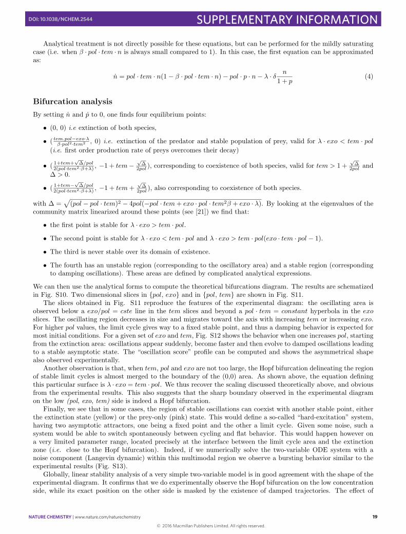
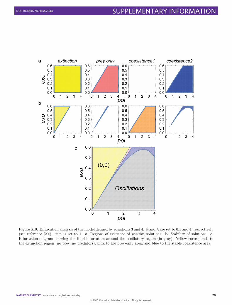
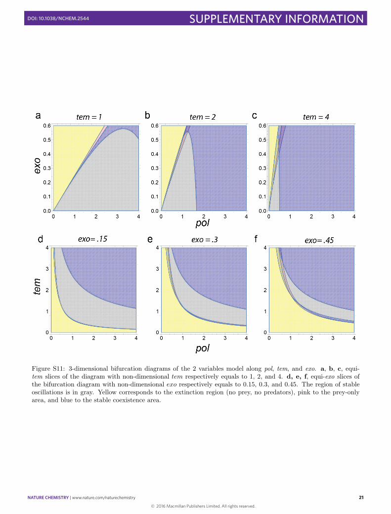
We can then use the analytical forms to compute the theoretical bifurcations diagram. The results are schematizedin Fig. S10. Two dimensional slices in {pol, exo} and in {pol, tem} are shown in Fig. S11.
The slices obtained in Fig. S11 reproduce the features of the experimental diagram: the oscillating area isobserved below a exo/pol = cste line in the tem slices and beyond a pol · tem = constant hyperbola in the exo
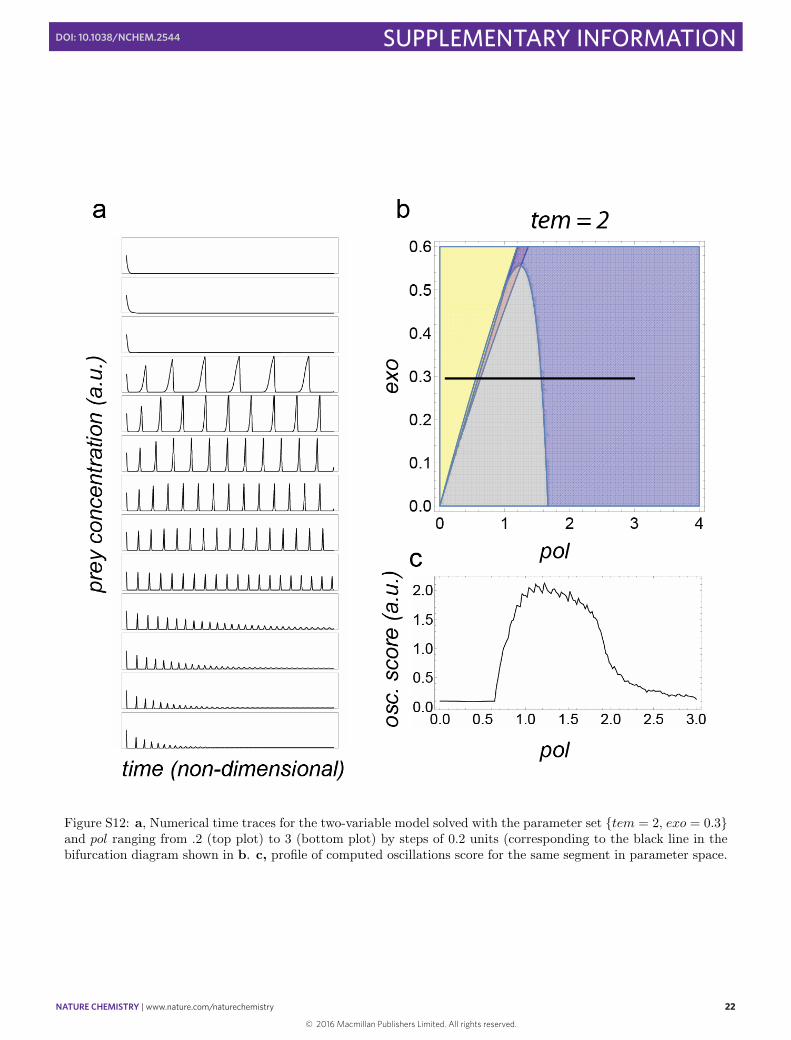
slices. The oscillating region decreases in size and migrates toward the axis with increasing tem or increasing exo.For higher pol values, the limit cycle gives way to a fixed stable point, and thus a damping behavior is expected formost initial conditions. For a given set of exo and tem, Fig. S12 shows the behavior when one increases pol, startingfrom the extinction area: oscillations appear suddenly, become faster and then evolve to damped oscillations leadingto a stable asymptotic state. The “oscillation score” profile can be computed and shows the asymmetrical shapealso observed experimentally.
Another observation is that, when tem, pol and exo are not too large, the Hopf bifurcation delineating the regionof stable limit cycles is almost merged to the boundary of the (0,0) area. As shown above, the equation definingthis particular surface is λ · exo = tem · pol. We thus recover the scaling discussed theoretically above, and obviousfrom the experimental results. This also suggests that the sharp boundary observed in the experimental diagramon the low (pol, exo, tem) side is indeed a Hopf bifurcation.
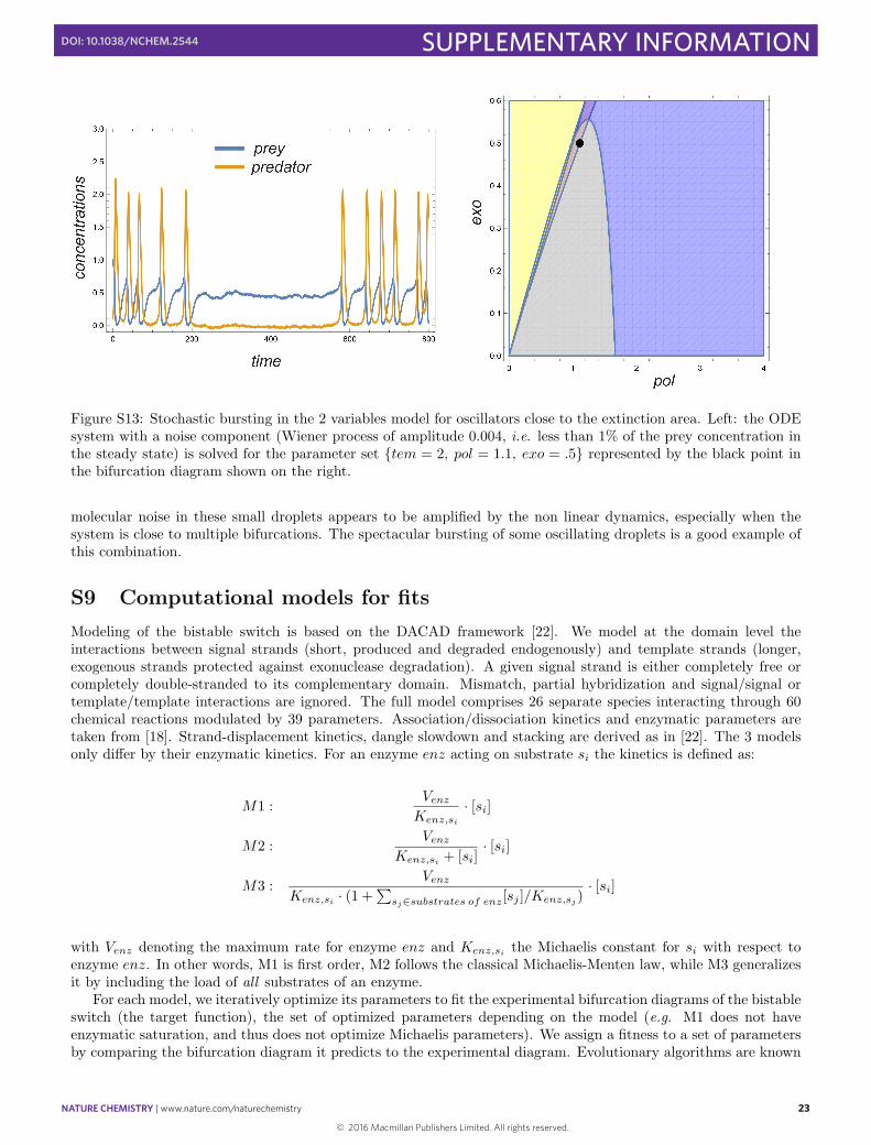
Finally, we see that in some cases, the region of stable oscillations can coexist with another stable point, eitherthe extinction state (yellow) or the prey-only (pink) state. This would define a so-called “hard-excitation” system,having two asymptotic attractors, one being a fixed point and the other a limit cycle. Given some noise, such asystem would be able to switch spontaneously between cycling and flat behavior. This would happen however ona very limited parameter range, located precisely at the interface between the limit cycle area and the extinctionzone (i.e. close to the Hopf bifurcation). Indeed, if we numerically solve the two-variable ODE system with anoise component (Langevin dynamic) within this multimodal region we observe a bursting behavior similar to theexperimental results (Fig. S13).
Globally, linear stability analysis of a very simple two-variable model is in good agreement with the shape of theexperimental diagram. It confirms that we do experimentally observe the Hopf bifurcation on the low concentrationside, while its exact position on the other side is masked by the existence of damped trajectories. The e↵ect of
19
© 2016 Macmillan Publishers Limited. All rights reserved.
NATURE CHEMISTRY | www.nature.com/naturechemistry 20
SUPPLEMENTARY INFORMATIONDOI: 10.1038/NCHEM.2544
Figure S10: Bifurcation analysis of the model defined by equations 3 and 4. β and λ are set to 0.1 and 4, respectively(see reference [20]). tem is set to 1. a, Regions of existence of positive solutions. b, Stability of solutions. c,Bifurcation diagram showing the Hopf bifurcation around the oscillatory region (in gray). Yellow corresponds tothe extinction region (no prey, no predators), pink to the prey-only area, and blue to the stable coexistence area.
20
© 2016 Macmillan Publishers Limited. All rights reserved.
NATURE CHEMISTRY | www.nature.com/naturechemistry 21
SUPPLEMENTARY INFORMATIONDOI: 10.1038/NCHEM.2544
Figure S11: 3-dimensional bifurcation diagrams of the 2 variables model along pol, tem, and exo. a, b, c, equi-tem slices of the diagram with non-dimensional tem respectively equals to 1, 2, and 4. d, e, f, equi-exo slices ofthe bifurcation diagram with non-dimensional exo respectively equals to 0.15, 0.3, and 0.45. The region of stableoscillations is in gray. Yellow corresponds to the extinction region (no prey, no predators), pink to the prey-onlyarea, and blue to the stable coexistence area.
21
© 2016 Macmillan Publishers Limited. All rights reserved.
NATURE CHEMISTRY | www.nature.com/naturechemistry 22
SUPPLEMENTARY INFORMATIONDOI: 10.1038/NCHEM.2544
Figure S12: a, Numerical time traces for the two-variable model solved with the parameter set {tem = 2, exo = 0.3}and pol ranging from .2 (top plot) to 3 (bottom plot) by steps of 0.2 units (corresponding to the black line in thebifurcation diagram shown in b. c, profile of computed oscillations score for the same segment in parameter space.
22
© 2016 Macmillan Publishers Limited. All rights reserved.
NATURE CHEMISTRY | www.nature.com/naturechemistry 23
SUPPLEMENTARY INFORMATIONDOI: 10.1038/NCHEM.2544
Figure S13: Stochastic bursting in the 2 variables model for oscillators close to the extinction area. Left: the ODEsystem with a noise component (Wiener process of amplitude 0.004, i.e. less than 1% of the prey concentration inthe steady state) is solved for the parameter set {tem = 2, pol = 1.1, exo = .5} represented by the black point inthe bifurcation diagram shown on the right.
molecular noise in these small droplets appears to be amplified by the non linear dynamics, especially when thesystem is close to multiple bifurcations. The spectacular bursting of some oscillating droplets is a good example ofthis combination.
S9 Computational models for fits
Modeling of the bistable switch is based on the DACAD framework [22]. We model at the domain level theinteractions between signal strands (short, produced and degraded endogenously) and template strands (longer,exogenous strands protected against exonuclease degradation). A given signal strand is either completely free orcompletely double-stranded to its complementary domain. Mismatch, partial hybridization and signal/signal ortemplate/template interactions are ignored. The full model comprises 26 separate species interacting through 60chemical reactions modulated by 39 parameters. Association/dissociation kinetics and enzymatic parameters aretaken from [18]. Strand-displacement kinetics, dangle slowdown and stacking are derived as in [22]. The 3 modelsonly di↵er by their enzymatic kinetics. For an enzyme enz acting on substrate s
i
the kinetics is defined as:
M1 :V
enz
K
enz,s
i
· [si
]
M2 :V
enz
K
enz,s
i
+ [si
]· [s
i
]
M3 :V
enz
K
enz,s
i
· (1 +P
s
j
2substrates of enz
[sj
]/Kenz,s
j
)· [s
i
]
with V
enz
denoting the maximum rate for enzyme enz and K
enz,s
i
the Michaelis constant for s
i
with respect toenzyme enz. In other words, M1 is first order, M2 follows the classical Michaelis-Menten law, while M3 generalizesit by including the load of all substrates of an enzyme.
For each model, we iteratively optimize its parameters to fit the experimental bifurcation diagrams of the bistableswitch (the target function), the set of optimized parameters depending on the model (e.g. M1 does not haveenzymatic saturation, and thus does not optimize Michaelis parameters). We assign a fitness to a set of parametersby comparing the bifurcation diagram it predicts to the experimental diagram. Evolutionary algorithms are known
23
© 2016 Macmillan Publishers Limited. All rights reserved.
NATURE CHEMISTRY | www.nature.com/naturechemistry 24
SUPPLEMENTARY INFORMATIONDOI: 10.1038/NCHEM.2544
to perform particularly well in such context as they require few assumptions on the search space. We use CMA-ES [23, 24] which locally approximates the fitness gradients through stochastic sampling and evaluates the fitnesssensitivity in order to avoid the pitfalls of premature convergence and flat fitness landscape. We further constrainthe search to a bounded region by assigning the worst fitness to individuals whose parameters exceed specifiedbounds (typically 10-fold variations for enzymatic parameters and 100-fold for other parameters). Penalizing suchindividuals allows us to skip unnecessary ODE evaluation (which gets prohibitively slow for unrealistic parameters).
We perform 10 runs for each model, one run typically comprising 2000 evaluations (i.e. diagram evaluation) over40 generations of 50 individuals. A shared set of 6 parameters (stabilization e↵ect of stacking on all 4 templates, aswell as the ratios pol/exo and nic/exo ) is optimized for all models. Five additional parameters (Michaelis constantsfor all enzyme/substrate combinations) are optimized for M2 and M3. Optimized parameters for each model, alongwith their default values, are shown in Supplementary Table 3. We accelerate the evaluation of bifurcation diagrams-a major computational bottleneck- by sparsing. First, we coarse-grain the experimental diagrams of Fig. 3c (goingfrom a s100×100 binning to a 20×20 binning). Secondly, we sparse these coarse diagrams by removing large andhomogenous regions around the frontiers (indicated in Fig. 3f, g, h), going from 400 points to s200 points. Sparsingspeeds up diagram computation and penalizes models that poorly approximate the positions of bifurcations. Thesparse diagram is simulated for a model time of 11 hours. We then evaluate the diagram fitness as follows:
fit =
sP([↵to↵],[βtoβ])2conditions
dist([↵to↵], [βtoβ])2
#conditions
with
dist([↵to↵], [βtoβ])2 = ([↵toiβ]l,exp,↵
− [↵toiβ]l,sim,↵
)2
+([βtoi↵]l,exp,↵
− [βtoi↵]l,sim,↵
)2
+([↵toiβ]l,exp,β
− [↵toiβ]l,sim,β
)2
+([βtoi↵]l,exp,β
− [βtoi↵]l,sim,β
)2
where [·]l
represents the concentration of loaded template (rescaled between 0 and 1 to match the fluorescenceshift) and #conditions is the total number of points in the 2 sparsed bifurcation diagrams. We thus use thesquare distance between the expected concentration of loaded inhibiting template (i.e. those with trigger, whichare contributing to most of the fluorescence) and their simulated concentrations for the given initial concentrationof templates ↵to↵ and βtoβ. Note that we sum over two di↵erent initial conditions (↵β = 10 and ↵β = 01), whichaccounts for the four terms. The deviation of the parameters (likelihood) is computed as follows:
likelihood =
Pp2param
| log10
(current value
p
initial value
p
)|
#param
with param the set of optimized parameters for a given model. After each optimization run, we keep the bestfitting solutions found at every generations (i.e. one candidate solution per generation). We then map them in the2D space (likelihood, fitness) and draw the Pareto fronts of models, i.e individuals such that no other individualhas simultaneously a better fitness and likelihood. Pareto fronts are commonly used in multi-objective optimization[25, 26] for identifying groups of candidate solutions that are optimal with respect to multiple criteria. A modelis said to dominate another if none of the potential solution on its Pareto front are dominated by solutions fromthe other model. Note that a model can dominate over a particular range of parameters and be dominated overanother.
All models share the same 39 parameters: initial conditions (4 signal species initial concentrations, 4 templateinitial concentrations, 3 enzyme concentrations), hybridization/denaturation parameters (hybridization rate, sta-bility of all signal species, stability penalty for inhibitor on their target template compared to their generatingtemplate, left and right dangle stability increase per template, stacking denaturation slowdown for every template,invasion rate of an inhibited template by the input and output) and Michaelis-Menten parameters (activity for eachenzyme, a total of five K
m
). Table 3 shows which parameters where optimized for each model, along with theirinitial values. Details about the simulated reactions and the parameters can be found in [22]. Note that uponreceiving a new enzymatic batch, we measure its activity and normalize its concentration to recover the same baseactivity as [18].
24
© 2016 Macmillan Publishers Limited. All rights reserved.

NATURE CHEMISTRY | www.nature.com/naturechemistry 25
SUPPLEMENTARY INFORMATIONDOI: 10.1038/NCHEM.2544
Enzymes Km (M2, M3) Michaelis-Menten parameters (nM)Km
pol
80Km
pol,displ
5.5Km
nick
30Km
exo,signal
440Km
exo,inhib
150Stacking slowdown Slowdown for the denaturation rate of input and output strands when both are present on(M1, M2, M3) a template separated by a nick, due to the stacking of adjacent base-pairs.↵to↵ 1βtoβ 1↵toiβ 1βtoi↵ 1Enzyme concentration Normalized compared to their concentrations in [18] .(M1, M2, M3)Polymerase 1Nickase 1
Table 3: Description and default values of optimized parameter. Candidate solutions always contain the parametersindicated for their model, in the order presented in this Table. Stacking slowdowns are hard to estimate or measureand left open for optimization. The impact of enzymes on the system depends partly on the relative - rather thanabsolute - concentrations of enzymes. As simultaneously optimizing all three concentrations may result in a correctbalance between enzyme concentrations but unrealistic values, we fixed the exonuclease concentration, and evolvedthe concentrations of the two other enzymes.
25
© 2016 Macmillan Publishers Limited. All rights reserved.
NATURE CHEMISTRY | www.nature.com/naturechemistry 26
SUPPLEMENTARY INFORMATIONDOI: 10.1038/NCHEM.2544
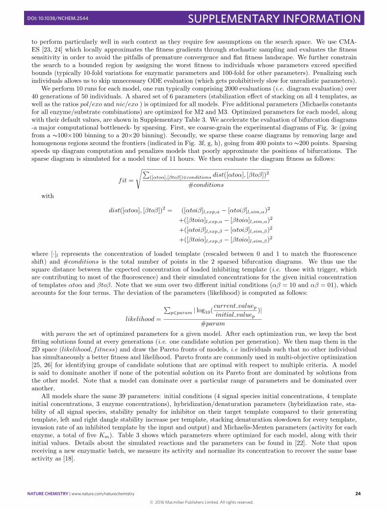
S10 Fluorescence images and histograms of the bistable switch
Figure S14: Fluorescence images of the barcode channels (parameter space). Top: Cascade Blue, coding for btob.Bottom: Alexa647, coding for atoa. These images correspond to the droplets generated for experiment of Fig. 3c(bistable circuit started in ab =01). The scale bar is 1 mm. The image contains about 10 000 droplets. Theirdiameter is 62 µm (+/- 10%). The brightest droplets correspond to the apex of the calibration arms.
26
© 2016 Macmillan Publishers Limited. All rights reserved.
NATURE CHEMISTRY | www.nature.com/naturechemistry 27
SUPPLEMENTARY INFORMATIONDOI: 10.1038/NCHEM.2544
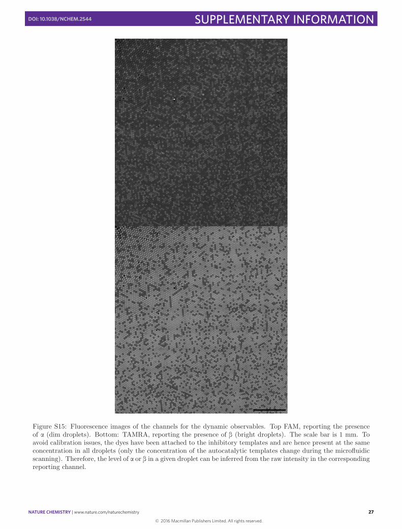
Figure S15: Fluorescence images of the channels for the dynamic observables. Top FAM, reporting the presenceof a (dim droplets). Bottom: TAMRA, reporting the presence of b (bright droplets). The scale bar is 1 mm. Toavoid calibration issues, the dyes have been attached to the inhibitory templates and are hence present at the sameconcentration in all droplets (only the concentration of the autocatalytic templates change during the microfluidicscanning). Therefore, the level of a or b in a given droplet can be inferred from the raw intensity in the correspondingreporting channel.
27
© 2016 Macmillan Publishers Limited. All rights reserved.
NATURE CHEMISTRY | www.nature.com/naturechemistry 28
SUPPLEMENTARY INFORMATIONDOI: 10.1038/NCHEM.2544
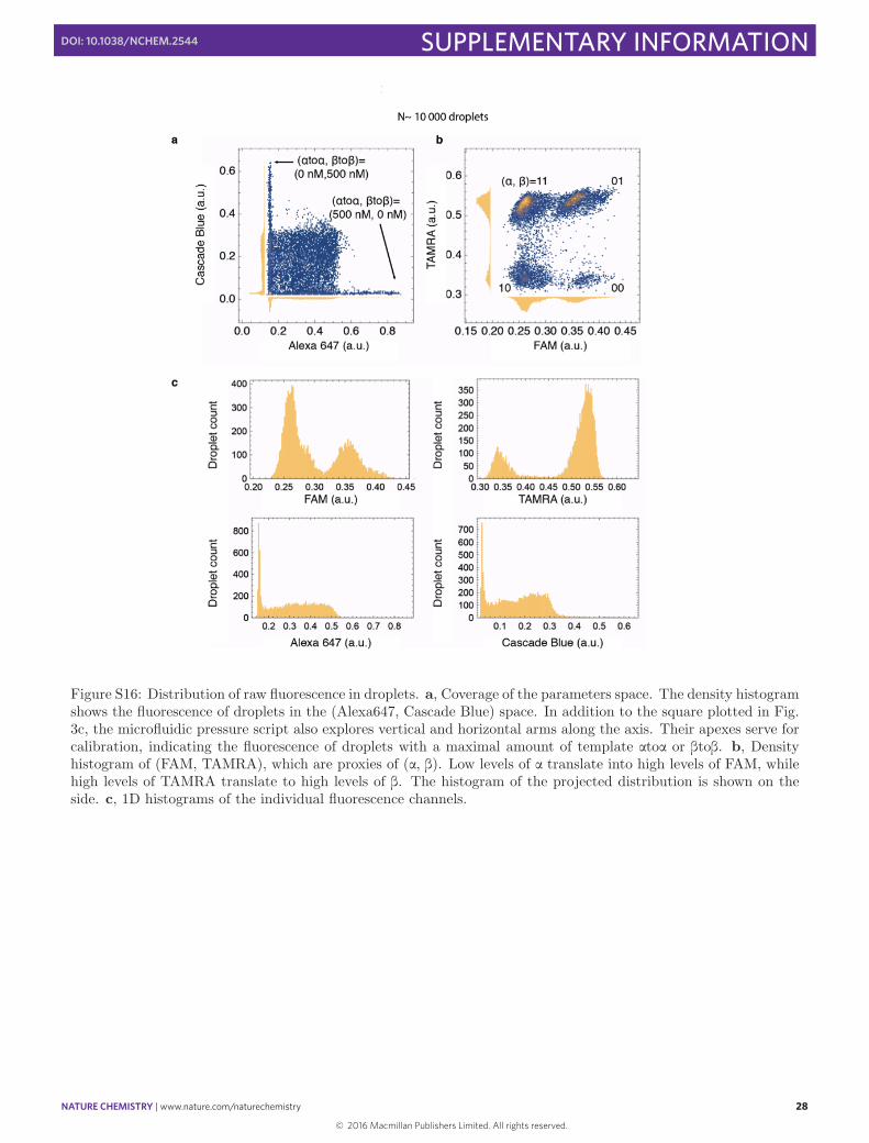
Figure S16: Distribution of raw fluorescence in droplets. a, Coverage of the parameters space. The density histogramshows the fluorescence of droplets in the (Alexa647, Cascade Blue) space. In addition to the square plotted in Fig.3c, the microfluidic pressure script also explores vertical and horizontal arms along the axis. Their apexes serve forcalibration, indicating the fluorescence of droplets with a maximal amount of template atoa or btob. b, Densityhistogram of (FAM, TAMRA), which are proxies of (a, b). Low levels of a translate into high levels of FAM, whilehigh levels of TAMRA translate to high levels of b. The histogram of the projected distribution is shown on theside. c, 1D histograms of the individual fluorescence channels.
28
© 2016 Macmillan Publishers Limited. All rights reserved.
NATURE CHEMISTRY | www.nature.com/naturechemistry 29
SUPPLEMENTARY INFORMATIONDOI: 10.1038/NCHEM.2544
S11 Droplet array and time traces for the predator-prey system
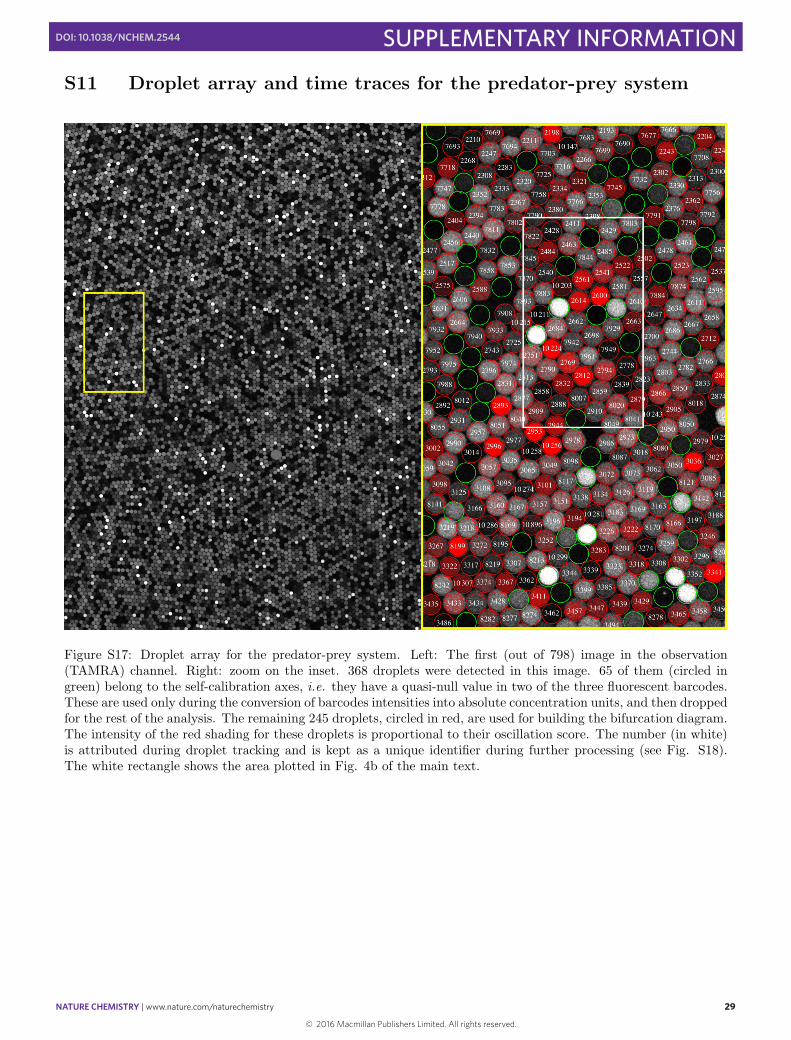
Figure S17: Droplet array for the predator-prey system. Left: The first (out of 798) image in the observation(TAMRA) channel. Right: zoom on the inset. 368 droplets were detected in this image. 65 of them (circled ingreen) belong to the self-calibration axes, i.e. they have a quasi-null value in two of the three fluorescent barcodes.These are used only during the conversion of barcodes intensities into absolute concentration units, and then droppedfor the rest of the analysis. The remaining 245 droplets, circled in red, are used for building the bifurcation diagram.The intensity of the red shading for these droplets is proportional to their oscillation score. The number (in white)is attributed during droplet tracking and is kept as a unique identifier during further processing (see Fig. S18).The white rectangle shows the area plotted in Fig. 4b of the main text.
29
© 2016 Macmillan Publishers Limited. All rights reserved.
NATURE CHEMISTRY | www.nature.com/naturechemistry 30
SUPPLEMENTARY INFORMATIONDOI: 10.1038/NCHEM.2544
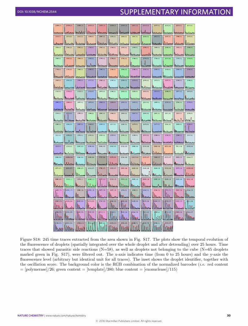
Figure S18: 245 time traces extracted from the area shown in Fig. S17. The plots show the temporal evolution ofthe fluorescence of droplets (spatially integrated over the whole droplet and after detrending) over 25 hours. Timetraces that showed parasitic side reactions (N=58), as well as droplets not belonging to the cube (N=65 dropletsmarked green in Fig. S17), were filtered out. The x-axis indicates time (from 0 to 25 hours) and the y-axis thefluorescence level (arbitrary but identical unit for all traces). The inset shows the droplet identifier, together withthe oscillation score. The background color is the RGB combination of the normalized barcodes (i.e. red content= [polymerase]/26; green content = [template]/380; blue content = [exonuclease]/115)
30
© 2016 Macmillan Publishers Limited. All rights reserved.
NATURE CHEMISTRY | www.nature.com/naturechemistry 31
SUPPLEMENTARY INFORMATIONDOI: 10.1038/NCHEM.2544
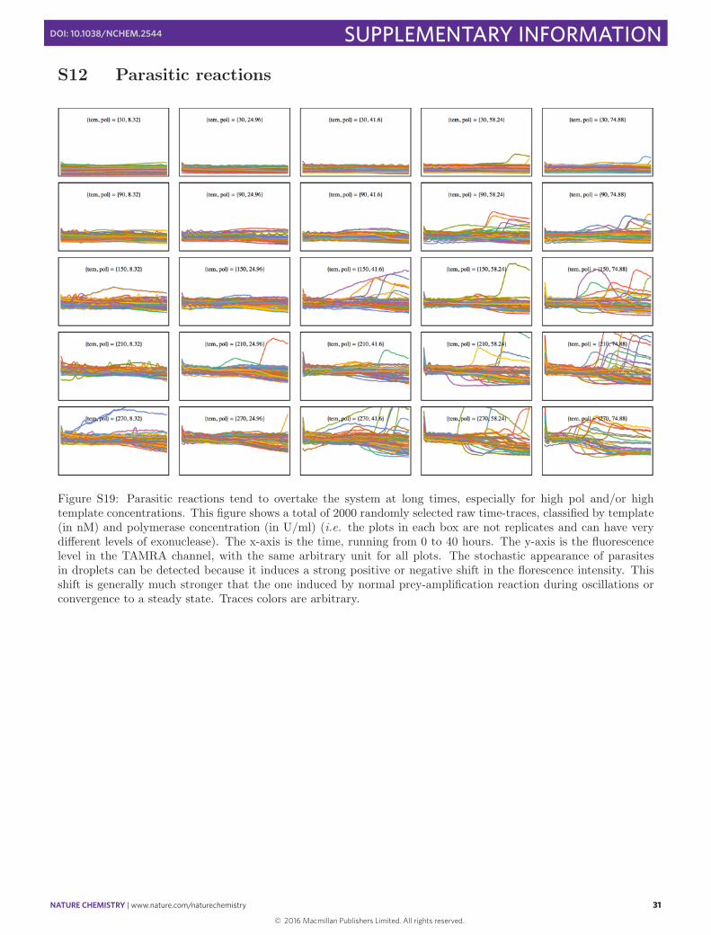
S12 Parasitic reactions
Figure S19: Parasitic reactions tend to overtake the system at long times, especially for high pol and/or hightemplate concentrations. This figure shows a total of 2000 randomly selected raw time-traces, classified by template(in nM) and polymerase concentration (in U/ml) (i.e. the plots in each box are not replicates and can have verydi↵erent levels of exonuclease). The x-axis is the time, running from 0 to 40 hours. The y-axis is the fluorescencelevel in the TAMRA channel, with the same arbitrary unit for all plots. The stochastic appearance of parasitesin droplets can be detected because it induces a strong positive or negative shift in the florescence intensity. Thisshift is generally much stronger that the one induced by normal prey-amplification reaction during oscillations orconvergence to a steady state. Traces colors are arbitrary.
31
© 2016 Macmillan Publishers Limited. All rights reserved.
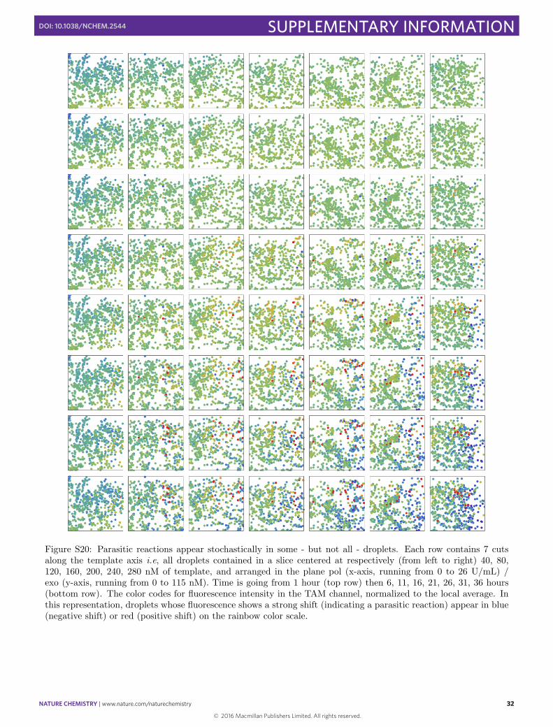
NATURE CHEMISTRY | www.nature.com/naturechemistry 32
SUPPLEMENTARY INFORMATIONDOI: 10.1038/NCHEM.2544
Figure S20: Parasitic reactions appear stochastically in some - but not all - droplets. Each row contains 7 cutsalong the template axis i.e, all droplets contained in a slice centered at respectively (from left to right) 40, 80,120, 160, 200, 240, 280 nM of template, and arranged in the plane pol (x-axis, running from 0 to 26 U/mL) /exo (y-axis, running from 0 to 115 nM). Time is going from 1 hour (top row) then 6, 11, 16, 21, 26, 31, 36 hours(bottom row). The color codes for fluorescence intensity in the TAM channel, normalized to the local average. Inthis representation, droplets whose fluorescence shows a strong shift (indicating a parasitic reaction) appear in blue(negative shift) or red (positive shift) on the rainbow color scale.
32
© 2016 Macmillan Publishers Limited. All rights reserved.
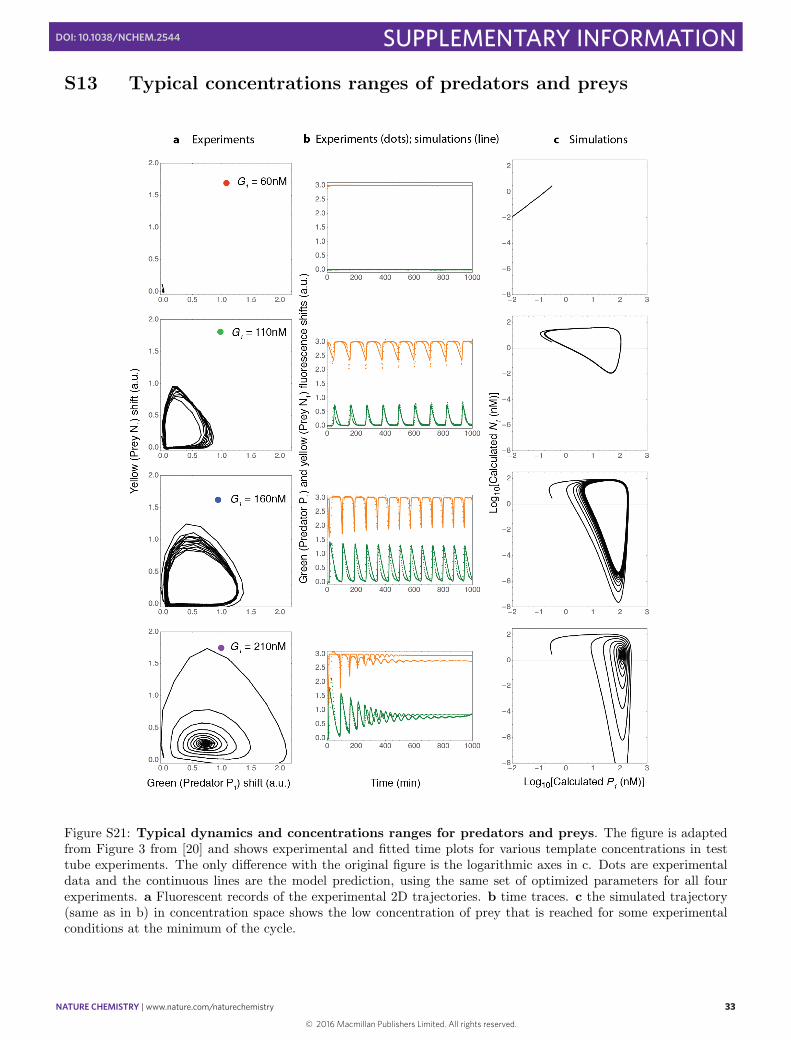
NATURE CHEMISTRY | www.nature.com/naturechemistry 33
SUPPLEMENTARY INFORMATIONDOI: 10.1038/NCHEM.2544
S13 Typical concentrations ranges of predators and preys
Figure S21: Typical dynamics and concentrations ranges for predators and preys. The figure is adaptedfrom Figure 3 from [20] and shows experimental and fitted time plots for various template concentrations in testtube experiments. The only di↵erence with the original figure is the logarithmic axes in c. Dots are experimentaldata and the continuous lines are the model prediction, using the same set of optimized parameters for all fourexperiments. a Fluorescent records of the experimental 2D trajectories. b time traces. c the simulated trajectory(same as in b) in concentration space shows the low concentration of prey that is reached for some experimentalconditions at the minimum of the cycle.
33
© 2016 Macmillan Publishers Limited. All rights reserved.
NATURE CHEMISTRY | www.nature.com/naturechemistry 34
SUPPLEMENTARY INFORMATIONDOI: 10.1038/NCHEM.2544
References
[1] A. Padirac, T. Fujii, and Y. Rondelez. Quencher-free multiplexed monitoring of dna reaction circuits. NucleicAcids Research, 40(15):e118, 2012.
[2] C. Holtze, A. C. Rowat, J. J. Agresti, J. B. Hutchison, F. E. Angile, C. H. J. Schmitz, S. Koster, H. Duan,K. J. Humphry, R. A. Scanga, J. S. Johnson, D. Pisignano, and D. A. Weitz. Biocompatible surfactants forwater-in-fluorocarbon emulsions. Lab on a Chip, 8(10):1632–1639, 2008.
[3] D. C. Du↵y, J. C. McDonald, O. J. A. Schueller, and G. M. Whitesides. Rapid prototyping of microfluidicsystems in poly(dimethylsiloxane). Analytical Chemistry, 70(23):4974–4984, 1998.
[4] S. Kaneda, K. Ono, T. Fukuba, T. Nojima, T. Yamamoto, and T. Fujii. Modification of the glass surfaceproperty in pdms-glass hybrid microfluidic devices. Analytical Sciences, 28(1):39–44, 2012.
[5] Jean-Christophe Baret, Felix Kleinschmidt, Abdeslam El Harrak, and Andrew D. Griffiths. Kinetic aspects ofemulsion stabilization by surfactants: A microfluidic analysis. Langmuir, 25(11):6088–6093, 2009.
[6] J. C. Lotters, W. Olthuis, P. H. Veltink, and P. Bergveld. The mechanical properties of the rubber elas-tic polymer polydimethylsiloxane for sensor applications. Journal of Micromechanics and Microengineering,7(3):145–147, 1997.
[7] Arthur D Edelstein, Mark A Tsuchida, Nenad Amodaj, Henry Pinkard, Ronald D Vale, and Nico Stuur-man. Advanced methods of microscope control using micro-manager software. Journal of Biological Methods,1(2):e11, 2014.
[8] K. Hasatani, M. Leocmach, A. J. Genot, A. Estevez-Torres, T. Fujii, and Y. Rondelez. High-throughput andlong-term observation of compartmentalized biochemical oscillators. Chemical Communications, 49(73):8090–8092, 2013.
[9] Buitelaar R.M., Bucke C., Tramper J., and Wij↵els R.H., editors. Immobilized Cells: Basics and Applications:Basics and Applications, page 202. Elsevier, 2006.
[10] G. L. Lukacs, P. Haggie, O. Seksek, D. Lechardeur, N. Freedman, and A. S. Verkman. Size-dependent dnamobility in cytoplasm and nucleus. Journal of Biological Chemistry, 275(3):1625–1629, 2000.
[11] Y. P. Bai, X. M. He, D. S. Liu, S. N. Patil, D. Bratton, A. Huebner, F. Hollfelder, C. Abell, and W. T. S.Huck. A double droplet trap system for studying mass transport across a droplet-droplet interface. Lab on aChip, 10(10):1281–1285, 2010.
[12] Maximilian Weitz, Jongmin Kim, Korbinian Kapsner, Erik Winfree, Elisa Franco, and Friedrich C. Simmel.Diversity in the dynamical behaviour of a compartmentalized programmable biochemical oscillator. NatureChemistry, 6(4):295–302, 2014.
[13] D. Pekin, Y. Skhiri, J. C. Baret, D. Le Corre, L. Mazutis, C. Ben Salem, F. Millot, A. El Harrak, J. B.Hutchison, J. W. Larson, D. R. Link, P. Laurent-Puig, A. D. Griffiths, and V. Taly. Quantitative and sensitivedetection of rare mutations using droplet-based microfluidics. Lab on a Chip, 11(13):2156–2166, 2011.
[14] Jung-uk Shim, Rohan T. Ranasinghe, Clive A. Smith, Shehu M. Ibrahim, Florian Hollfelder, Wilhelm T. S.Huck, David Klenerman, and Chris Abell. Ultrarapid generation of femtoliter microfluidic droplets for single-molecule-counting immunoassays. Acs Nano, 7(7):5955–5964, 2013.
[15] J. C. Baret, O. J. Miller, V. Taly, M. Ryckelynck, A. El-Harrak, L. Frenz, C. Rick, M. L. Samuels, J. B.Hutchison, J. J. Agresti, D. R. Link, D. A. Weitz, and A. D. Griffiths. Fluorescence-activated droplet sorting(fads): efficient microfluidic cell sorting based on enzymatic activity. Lab on a Chip, 9(13):1850–1858, 2009.
[16] Siavash Kijani, Ulf Yrlid, Maria Heyden, Malin Levin, Jan Boren, and Per Fogelstrand. Filter-dense multicolormicroscopy. Plos One, 10(3), 2015.
[17] J. N. Zadeh, C. D. Steenberg, J. S. Bois, B. R. Wolfe, M. B. Pierce, A. R. Khan, R. M. Dirks, and N. A. Pierce.Nupack: Analysis and design of nucleic acid systems. Journal of Computational Chemistry, 32(1):170–173,2011.
34
© 2016 Macmillan Publishers Limited. All rights reserved.

NATURE CHEMISTRY | www.nature.com/naturechemistry 35
SUPPLEMENTARY INFORMATIONDOI: 10.1038/NCHEM.2544
[18] A. Padirac, T. Fujii, and Y. Rondelez. Bottom-up construction of in vitro switchable memories. Proceedingsof the National Academy of Sciences of the United States of America, 109(47):E3212–E3220, 2012.
[19] Lei Dai, Daan Vorselen, Kirill S. Korolev, and Je↵ Gore. Generic indicators for loss of resilience before atipping point leading to population collapse. Science, 336(6085):1175–1177, 2012.
[20] T. Fujii and Y. Rondelez. Predator-prey molecular ecosystems. Acs Nano, 7(1):27–34, 2013.
[21] J.D Murray. Mathematical Biology, volume 17 of Interdisciplinary Applied Mathematics. Springer, third edition,2004.
[22] Nathanael Aubert, Clement Mosca, Teruo Fujii, Masami Hagiya, and Yannick Rondelez. Computer-assisteddesign for scaling up systems based on dna reaction networks. Journal of the Royal Society Interface, 11(93),2014.
[23] N. Hansen, S. D. Muller, and P. Koumoutsakos. Reducing the time complexity of the derandomized evolutionstrategy with covariance matrix adaptation (cma-es). Evolutionary Computation, 11(1):1–18, 2003.
[24] N. Hansen and A. Ostermeier. Completely derandomized self-adaptation in evolution strategies. EvolutionaryComputation, 9(2):159–195, 2001.
[25] R. T. Marler and J. S. Arora. Survey of multi-objective optimization methods for engineering. Structural andMultidisciplinary Optimization, 26(6):369–395, 2004.
[26] A. E. Eiben and James E. Smith. Introduction to Evolutionary Computing. Natural Computing Series. Springer,2015.
35
© 2016 Macmillan Publishers Limited. All rights reserved.