Summary Measures of Population Health:Methods for Calculating Healthy Life Expectancy

Michael T. Molla, Ph.D.; Diane K. Wagener, Ph.D.; and Jennifer H. Madans, Ph.D.

Number 21 August 2001

AbstractThis report is one of several appearing as HealthyPeople Statistical Notes that evaluate methodologicalissues pertaining to summary measures. Summarymeasures of population health are statistics thatcombine mortality and morbidity to represent overallpopulation health in a single number—in this report,health expectancy measures. This report presents acomprehensive discussion of the methods forcalculation and methodologic issues related to theinterpretation of healthy life expectancy. Thesemeasures combine both mortality and morbidity usingan abridged life-table procedure. Data from theNational Center for Health Statistics and other sourceswill be used to illustrate the calculation of the statisticsand the associated statistical tests.

Key words: summary measures c compression ofmorbidity c life table c life expectancy c healthy lifeexpectancy c healthy years.

IntroductionFor the populations of the industrialized nations of the

world, the 20th century has been a period of bothdemographic and epidemiologic transitions. In addition tothe substantial decrease in fertility during this period, allindustrialized countries experienced huge declines in crudedeath rates and infant mortality rates. This resulted in animpressive rise in the average life expectancy. For example,in the United States during the first half of the century, theaverage expectation of life at birth for the total populationincreased by nearly 45 percent—from 47.3 years in 1900 to68.2 years by 1950 (1), a gain of nearly 21 years. In thesecond half of the century, mortality in the United Statescontinued to decline, though at a much slower rate comparedwith the first half of the century. For example, from1950–98 the average expectation of life at birth increasedfrom 68.2 to 76.7 years, a gain of only 8.5 years.

The substantial gain in life expectancy during the firsthalf of the century caused a dramatic change in the agestructures of the populations of these industrialized countriesin the second half of the century. The longer average lifespan meant a sharp rise in the percent of the elderlypopulation. There was also a sharp rise in noncommunicable

Mortality component:

Age-specific death rates

Summary measure of population health:

Healthy life expectancy or healthy life years

-

Morbidity component:

Population morbidity, disability, or health-related quality of life

SOURCE: Adapted from a model by the Institute of Medicine, National Academy of

Sciences (2).

Life table technique

Figure 1. A schematic presentation of the model

chronic and degenerative diseases primarily affecting the older population. In the United States, the combined effect of these changes has encouraged a shift in focus from longevity to preventing disability, improving functioning, and relieving physical pain and emotional distress (2). This also meant that population health measures were needed to account for morbidity as well as longevity (3). One group of measures that included both of these components are health measures broadly known as ‘‘healthy life expectancy’’ (HLE).

Healthy Life Expectancy The development of health measures that include both

mortality and morbidity conditions of the population has been a focus of study since the 1960’s. After Sanders published the results of his research on measuring community health levels (4), HLE estimates were published by the U.S. Department Health, Education, and Welfare for the first time in 1969 (5). Sullivan (6) later published the methods for calculating these estimates. At that time, the World Health Organization (WHO) noted that the fundamental objective of human activity should include both long life as well as good health. They expanded the definition of health as ‘‘a state of complete physical, mental and social well-being.’’ Both WHO and the Organization for Economic Cooperation and Development reported on healthy life (7). In 1974, WHO recommended that ‘‘person-years of life in health’’ be calculated and be compared with the total person-years of life (8).

In the 1980’s, two new concerns became important, the relationship between changes in mortality and morbidity and the relatively greater burden of morbidity in the older ages. Debate centered on whether the factors responsible for the reductions in mortality would have a similar effect on morbidity. Some argued that most of the years of life that the elderly gained due to the decline of mortality were ‘‘healthy years’’ because morbidity was being pushed to the last few years of life, the compression of morbidity (9, 10). Others argued that the mortality decline observed over the past several decades was more likely to be the result of improvements in health care that saved more lives rather than either disease prevention that maintains healthy states or medical care that delays functional consequences of disease (11).

At the same time, Manton (12) introduced the concept of dynamic equilibrium. The theory of dynamic equilibrium is that chronic diseases have become less of a problem because deterioration in health due to disease has slowed down. The argument further suggested that while the decrease in mortality might have contributed to an increase in the prevalence of chronic diseases, these diseases would be of milder character leading to an overall better quality of life. Clearly, the issues related to the compression of morbidity further made clear that health status was a consequence of an interaction between mortality and morbidity, both at the micro and macro levels.

- 2 -

Encouraged by the basic idea of developing health measures that incorporate mortality and morbidity and motivated by the concept of compressing morbidity, health researchers continued to study empirical and methodologic issues throughout the 1990’s (see appendix). Empirical studies estimated healthy life expectancy indexes based on a variety of health attributes. The name given the various HLE indexes depends on methods by which different health states are measured (13). When health states are measured based on broadly defined chronic or acute morbid conditions, the more general name ‘‘healthy years’’ or ‘‘healthy life expectancy’’ is used . However, when health states are defined based on social or functional limitation, the estimated index is called ‘‘disability-free life expectancy.’’ When health states are measured by activity limitation, the index is often called ‘‘active life expectancy.’’

Components of Healthy Life Years The estimation of healthy life expectancy is based on

the concept of a closed population within a given period of time, that is, a population with no immigration or emigration. The period of time may be of any length, but the most commonly used period is one year. At the end of the year, the population can be partitioned into those who died within the period and those who are still alive. Of those still alive, the majority are expected to be healthy, and some are expected to be unhealthy. Hence, a model can be built that measures the health status of persons who are alive at the same time it accounts for those who die in the period of time. Such a model is schematically presented in figure 1.

According to this model, healthy life expectancy is a summary measure of a population composed of two sets of partial measures. The first set of measures, the age-specific death rates, accounts for the mortality component. The second set of measures, the age-specific rates of population

Mortality data

Midyear

population

estimates

Health data

Age-specific death

rates

Life table

technique

U.S. Bureau

of the Census

Self-assessed health

(poor or fair)

(

( D )5

5

5

x

x

x(1- )

Self-assessed health

(good or better)

Healthy life

expectancy

NCHS

NCHS

Data sources Data Calculation Index

NOTES: NCHS is the National Center for Health Statistics. Variables are defined in tables 1-5.

)

Figure 2. A schematic framework for estimating healthy life expectancy at the national level using respondent-assessed health status as an example

HEALTH

Emotional function

Depth of

coverage

Physical function

Sensory function

Pain Cognitive ability

Mobility Physical activity

Self-care Role performance

Breadth of coverage

morbidity, disability, or health-related quality of life,1

accounts for the morbidity component. These two components are combined using a mathematical function thattransforms the two sets of partial measures into a single composite measure using a life table methodology. Figure 2 displays the framework of this calculation, including the typeof data needed and the techniques used to estimate the two components of the measure at the national level.

At the national level, the mortality data are obtained from the National Vital Statistics System of the National Center for Health Statistics (NCHS), Centers for Disease Control and Prevention. Mortality data are collected by each state and the District of Columbia and compiled at the national level by NCHS. Midyear population estimates are from the U.S. Bureau of the Census.

Health data can come from a number of different sources depending on the type of health measure and the population being considered. Boyle and Torrance (14) developed a ‘‘health state classification system’’ (displayed in part in figure 3). Only some health attributes are interrelated. Hence, attributes can be classified to show similarities and differences. The classification system of Boyle and Torrance conceptualizes the interrelationship of health attributes as hierarchal, based on breadth and on coverage of different aspects of health. For example, physical function, which is one of the primary-level health

1Health related quality of life (HRQOL) refers to the effect of health conditions on function. It focuses on the qualitative dimension of functioning and incorporates duration of stay in various health states (Kaplan and Anderson (15)).

- 3

attributes, has four secondary-level attributes, one of which is self-care. Self-care may, in turn, be disaggregated into more specific health attributes, shown as the third level of classification in figure 3. The interpretation of the HLE depends on the health data used to estimate the statistic.

Because national data for respondent-assessed health are evaluated in the example presented here, the National Health Interview Survey (NHIS) conducted by NCHS is used. To calculate the age-specific prevalence rates of being healthy,

Bathing Continence Eating Dressing

SOURCE: Adapted from Boyle and Torrance (14).

Figure 3. An example of a classification system for health attributes

-

2Mortality rates for age 0 and age group 1–4 are calculated separately when knowing ‘‘their pattern in more detail’’ is preferred (22).

first calculate the rates of reporting ‘‘fair or poor’’ health (nπx). The rates of being healthy, that is, reporting ‘‘good or better’’ health is then (1−nπx). Then for each age interval (x, x+n), the rates of being healthy (1−nπx) are multiplied with the total number of years lived within the same age interval (nLx) to estimate the total number of years a group of persons is expected to live in a healthy state during the interval. The age interval (x, x+n) is equal to 1 if data used are in single-year age groups, or 5 or 10 if data used are in 5- or 10-year age groups.

The model used to estimate healthy life expectancy (i.e., the expected number of years in good or better health) is:

w1

e′ x = ∑ (1−nπx) nLilx i=x (1)

where

ex ′ is healthy life expectancy at age x, or the number of remaining years of healthy life for persons who have reached age x

lx is the number of survivors at age x

(1−nπx) represents the age-specific rate of being healthy

nLx is the total number of years lived by a cohort in the age interval (x, x+n)

w is the oldest age category

HLE could be estimated using a variety of health attributes. For example, the model may be used to estimate disability-free life expectancy or life without activity limitation, also referred to as expected years of active life. Regardless of the health attribute chosen, however, the model uses two separate and independent partial health measures: (1−nπx) for the morbidity component and lx and

nLx for the mortality component.

Life Table Technique The life table, also known as the mortality table, is

used to present the most complete statistical description of mortality (16). The life table has also been an important tool of demographers who are interested in estimating the probability of marriage and remarriage, widowhood, becoming an orphan, and migration and population projections (17). In addition to the analyses of mortality and other demographic characteristics of human populations, the life table technique has been used to measure decrements in nonhuman groups or aggregates, including animals, insects, cases of illness, or even items of industrial equipment (18). The technique has been used to estimate risks and insurance benefits and school life (19), and even used to analyze prime time programs on a television network (20).

The method of calculating HLE is presented in this report in four parts. Healthy life expectancy is a modified life expectancy calculation. Therefore, the method is best presented by showing the calculations of life expectancy and discussing the modifications. Part I addresses the estimation

- 4

of life table values. Part II presents the estimation of age-specific prevalence rates of health states and how the two partial measures of the mortality and morbidity components are combined to estimate the final age-specific composite health measure. Part III covers the estimation of the standard errors of healthy life expectancy. Part IV explains the application of the estimated healthy life expectancy and the associated standard errors in the statistical testing of health disparity between population subgroups.

Estimating Average Life Expectancy

The objective of the life table is to calculate the expected life expectancy of groups of people currently at specified ages if they lived the rest of their lives experiencing the age-specific mortality rates observed for the population at a specific time. The technique, therefore, uses the age-specific mortality to calculate the proportion of people alive at the beginning of an age interval who die before reaching the next age group. The average number of person-years lost because of those deaths is then subtracted from the total possible person-years for the age group of the cohort. These person-years are then added for all the age groups being considered to yield the expected number of years remaining. The method for constructing a complete annual life table is discussed in another NCHS publication (21).

The estimation of life table values, such as the expectation of life, begins with the computation of age-specific death rates. An illustrative example is presented in table 1 using 1995 data for white females in the United States. The two sets of data required to construct a life table are the midyear population and the number of deaths in that year. These data could be analyzed in single years of age or 5- or 10-year age groups. The process could be applied to the construction of a life table for national, state, or local populations.

In the first column, the age groups are listed. In the example shown in table 1, the initial 5-year age group is 0–4 years2 and the final age groups is 85 years and over. The determining factor for the age grouping is the availability and quality of data. It should be noted that the age that begins the final age group (also known as the open age interval) does not have any effect on the life table being constructed.

The next two columns of the table give counts for the population nPx and deaths nDx for each age group. The population counts are based on midyear estimates. The deaths are for the entire year. These are used to compute the average death rate of each age-group for the year (nMx, where n, the number of years in the age groups is 5 in table 1), as

nMx = nDx / nPx (2)

-

Table 1. Life table for white females: United States, 1995

Proportion Probability Total Number of Life Age- of years lived of dying Number number of years lived expectancy

Number specific by those who during age alive at the years lived in this and at beginning Age Mid-year of deaths die in age interval beginning of in age subsequent of age

interval1 population deaths per 1,000 interval2 age interval interval age intervals interval

x to x+5 5Px 5Dx 5Mx ax 5qx lx 5Lx Tx ex

0–4 years . . . . . . . . . . . . . . . . . 7,530,865 10,277 1.3647 0.178 0.0068 100,000 497,211 7,945,930 79.5

5–9 years . . . . . . . . . . . . . . . . . 7,375,960 1,112 0.1508 0.477 0.0008 99,321 496,412 7,448,720 75.0

10–14 years . . . . . . . . . . . . . . . 7,294,788 1,335 0.1830 0.530 0.0009 99,247 496,020 6,952,308 70.1

15–19 years . . . . . . . . . . . . . . . 7,010,351 3,084 0.4400 0.555 0.0022 99,156 495,294 6,456,288 65.1

20–24 years . . . . . . . . . . . . . . . 7,020,389 3,102 0.4419 0.517 0.0022 98,938 494,163 5,960,994 60.3

25–29 years . . . . . . . . . . . . . . . 7,583,792 4,067 0.5363 0.519 0.0027 98,720 492,962 5,466,831 55.4

30–34 years . . . . . . . . . . . . . . . 8,918,195 6,554 0.7349 0.538 0.0037 98,455 491,441 4,973,870 50.5

35–39 years . . . . . . . . . . . . . . . 9,190,371 9,651 1.0501 0.524 0.0052 98,094 489,247 4,482,429 45.7

40–44 years . . . . . . . . . . . . . . . 8,478,260 12,541 1.4792 0.524 0.0074 97,580 486,191 3,993,182 40.9

45–49 years . . . . . . . . . . . . . . . 7,485,773 17,056 2.2784 0.528 0.0113 96,861 481,715 3,506,991 36.2

50–54 years . . . . . . . . . . . . . . . 5,969,413 22,572 3.7813 0.531 0.0187 95,764 474,612 3,025,276 31.6

55–59 years . . . . . . . . . . . . . . . 4,913,335 29,877 6.0808 0.534 0.0300 93,969 463,278 2,550,664 27.1

60–64 years . . . . . . . . . . . . . . . 4,570,327 44,926 9.8300 0.534 0.0480 91,152 445,546 2,087,386 22.9

65–69 years . . . . . . . . . . . . . . . 4,728,330 71,430 15.1068 0.534 0.0730 86,772 419,113 1,641,841 18.9

70–74 years . . . . . . . . . . . . . . . 4,451,633 105,434 23.6844 0.539 0.1123 80,441 381,366 1,222,727 15.2

75–79 years . . . . . . . . . . . . . . . 3,573,206 134,299 37.5850 0.543 0.1730 71,408 328,775 841,361 11.8

80–84 years . . . . . . . . . . . . . . . 2,603,800 163,724 62.8788 0.529 0.2739 59,051 257,187 512,586 8.7

85 years and over . . . . . . . . . . . . 2,405,023 349,118 145.1620 0.596 1.0000 42,880 255,399 255,399 6.0

1Mortality rates for those less than 1 year and age group 1–4 years are calculated separately when knowing ‘‘their pattern in more detail’’ is preferred (22). 2For a more detailed discussion of ax, see DHEW (24) and Keyfitz (27).

The computed age-specific death rates need to be checked for stability. Age-specific death rates are considered to be stable if they are based on 20 or more deaths. Rates based on fewer than 20 deaths have a relative standard error of 23 percent or more and therefore are considered highly variable (23).

The conditional probability of dying within a given age group nqx is given in column 6. This is the proportion of people in the age group alive at the beginning of the age interval who die before reaching the next age group. Whereas nMx is an annual death rate, nqx is a conditional probability of dying. This probability is estimated as:

nqx = [n c nMx ] / [1+n(1−ax) nMx] (3)

where ax is average proportion of years lived by those who died in this age interval (given in column 5). The conditional probability of dying is assumed to be 1.0 for the open, oldest age interval. In the example presented here, n is 5 years, so the probability becomes:

5qx = [5 c 5Mx] / [1+5(1−ax) 5Mx ]

The values for ax are constants derived from the complete U.S. life tables of 1949–51 (24). For single-year life table value calculations, ax may be assumed to be ½.

Having calculated the conditional probability of dying, one can now calculate the probability of surviving to an exact age marking the beginning of an interval. In the life table, this is expressed as the number of persons surviving to an exact age (or the exact age at the beginning of an age interval when group data are used), starting with an assumed cohort population (l0) frequently expressed as 100,000 at

- 5

birth (column 7). For any other specific age, the number of survivors at that age, (lx) can be calculated. Hence, the number alive at exact age x+n (lx+n) is calculated by multiplying the number of survivors at exact age x (lx) by the probability of surviving from age x to age x+n (1−nqx) or:

lx+n = lx (1−nqx ) (4)

The total number of person-years lived for those people who began the age interval x to x+n (column 8) is then the sum of the total number of years lived by individuals surviving to the end of the age interval plus the total number of years lived by those who die in the age interval. This becomes:

nLx = n [lx+n + ax (lx − lx+n)] (5)

In the example presented here, n = 5 so,

5Lx = 5 [lx+5 + ax (lx − lx+5)]

Column 9, the person-years remaining for the population, that is, Tx, is the total of all the person-years for age x and all subsequent age groups, or:

Tx = ∑ Li i=x

for i = x, x+n, ... , oldest age group (6)

The average per person expected years (column 10) is the total person-years divided by the number of persons surviving to the beginning of the age interval x, or:

ex = Tx / lx (7)

-

Table 2. Calculation of healthy life expectancy for white females by Sullivan’s method using abridged life table: United States, 1995

Number of Average number Proportion of years lived in of years in

Number alive Number of persons in age Proportion of Number of healthy state in healthy state at the years interval in state persons in age healthy years this and all remaining at

beginning of lived in considered interval in lived in subsequent age beginning of Age interval each interval age interval unhealthy healthy state age intervals intervals age interval

x to x+5 lx 5Lx 5πx (1−5πx ) ′

5Lx ′ T x

′ ex

0–4 years . . . . . . . . . . . . . . . . . 100,000 497,211 0.0185 0.9815 488,012 6,981,686 69.8

5–9 years . . . . . . . . . . . . . . . . . 99,321 496,412 0.0196 0.9804 486,682 6,493,674 65.4

10–14 years . . . . . . . . . . . . . . . 99,247 496,020 0.0189 0.9811 486,645 6,006,992 60.5

15–19 years . . . . . . . . . . . . . . . 99,156 495,294 0.0435 0.9565 473,749 5,520,347 55.7

20–24 years . . . . . . . . . . . . . . . 98,938 494,163 0.0490 0.9510 469,949 5,046,598 51.0

25–29 years . . . . . . . . . . . . . . . 98,720 492,962 0.0617 0.9383 462,546 4,576,649 46.4

30–34 years . . . . . . . . . . . . . . . 98,455 491,441 0.0614 0.9386 461,266 4,114,103 41.8

35 –39 years . . . . . . . . . . . . . . . 98,094 489,247 0.0773 0.9227 451,428 3,652,837 37.2

40–44 years . . . . . . . . . . . . . . . 97,580 486,191 0.0890 0.9110 442,920 3,201,409 32.8

45–49 years . . . . . . . . . . . . . . . 96,861 481,715 0.1094 0.8906 429,015 2,758,489 28.5

50–54 years . . . . . . . . . . . . . . . 95,764 474,612 0.1506 0.8494 403,136 2,329,473 24.3

55–59 years . . . . . . . . . . . . . . . 93,969 463,278 0.1919 0.8081 374,375 1,926,338 20.5

60–64 years . . . . . . . . . . . . . . . 91,152 445,546 0.2031 0.7969 355,055 1,551,963 17.0

65–69 years . . . . . . . . . . . . . . . 86,772 419,113 0.2257 0.7743 324,520 1,196,908 13.8

70–74 years . . . . . . . . . . . . . . . 80,441 381,366 0.2364 0.7636 291,211 872,388 10.8

75–79 years . . . . . . . . . . . . . . . 71,408 328,775 0.2782 0.7218 237,310 581,177 8.1

80–84 years . . . . . . . . . . . . . . . 59,051 257,187 0.3298 0.6702 172,367 343,867 5.8

85 years and over . . . . . . . . . . . . 42,880 255,399 0.3285 0.6715 171,501 171,501 4.0

Therefore, in the example presented in table 1, the expected number of years of life at birth (e0) is 79.5 years, the expected number of years of life at age 20 years (e20) is 60.3 years, and the expected number of years of life at age 65 years (e65) is 18.9 years.

Estimating Average Years of Healthy Life

The life table technique is a powerful tool for estimating the remaining years of life that a group of persons can expect to live once they had reached a certain age. Regardless of their age, the remaining years of life might be lived in good health, in less optimal health status, or some combination of both. The traditional life table technique does not distinguish between remaining healthy years and unhealthy years. Additional data are needed to disaggregate the total number of years into expected years of healthy and of unhealthy life.

Using health data, the total number of expected years of life are separated into healthy and unhealthy years (see figure 2). In general, health data, collected through health surveys or from clinical observations, are used to estimate the prevalence of different levels of health status. The population is then partitioned into proportions that are experiencing varying levels of health status. The separation may be as simple as dividing the population into those who are healthy or unhealthy. Or the population may be separated into more than two population subgroups according to varying levels of health status using multidimensional scaling to describe health status.

To calculate the HLE, the population of each age interval in the life table is separated into the proportion

- 6

experiencing an unhealthy condition (nπx) and those considered as healthy (1−nπx). An example is shown in columns 4 and 5 of table 2. Because nLx is the total number of person-years lived for the population in age interval x to x+n (equation 5), the proportion of these years lived in a

′ healthy state ( nLx) is then:

′ nLx = (1−nπx) nLx (8)

This is shown in column 6 of table 2. Equations (6) and (7) can then be used to obtain the healthy life expectancy (see column 8 of table 2) from the number of healthy person-years determined in (8) or

w1′ ′ ex = ∑ nLilx i=x (9)

′ The expected years of unhealthy life are ex− ex . However, if multiple states of health status are described, the prevalence for each of those states for each age interval must be calculated and equations similar to (8) and (9) are used to estimate separately the expected years of life in those health states.

In table 2, the health states have been defined using respondent-assessed health, which is obtained from health interview surveys using the question, ‘‘Would you say your health in general is excellent, very good, good, fair or poor’’ with five response categories: excellent, very good, good, fair, and poor. Health states are then defined as two mutually exclusive states: self-assessed health as poor or fair (column 4) and self-assessed health as good or better (column 5). The number of survivors at exact age x (lx) and number of

-

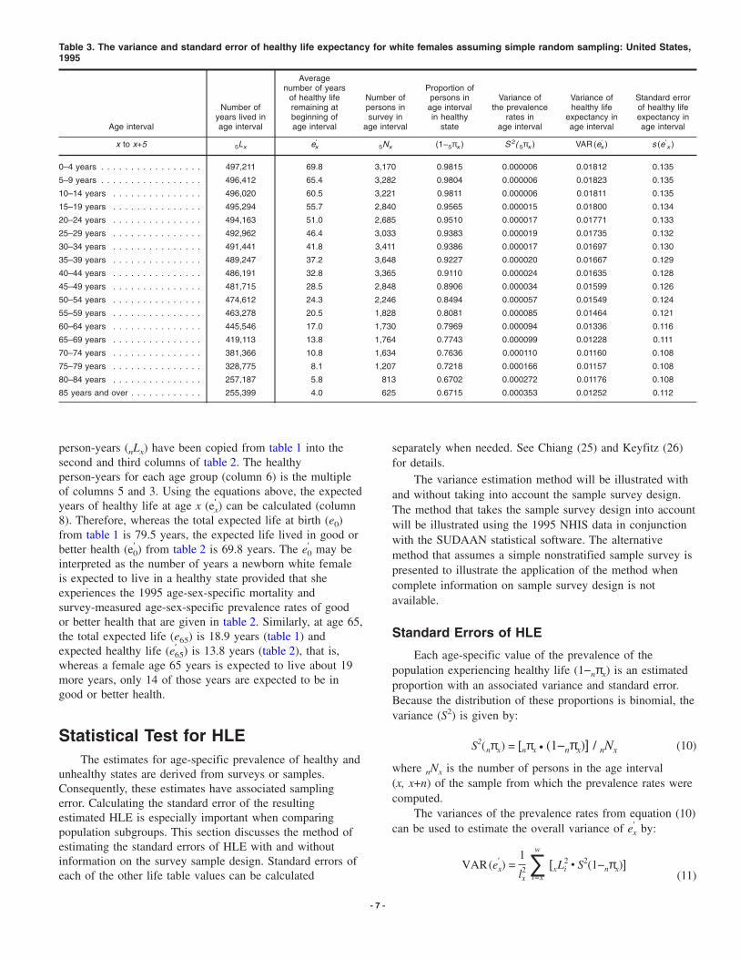
Table 3. The variance and standard error of healthy life expectancy for white females assuming simple random sampling: United States, 1995

Average number of years Proportion of

of healthy life Number of persons in Variance of Variance of Standard error Number of remaining at persons in age interval the prevalence healthy life of healthy life

years lived in beginning of survey in in healthy rates in expectancy in expectancy in Age interval age interval age interval age interval state age interval age interval age interval

′ ′ x to x+5 5Lx ex 5Nx (1−5πx ) S 2( 5πx ) VAR (ex ) s (e ′ x )

0–4 years . . . . . . . . . . . . . . . . . 497,211 69.8 3,170 0.9815 0.000006 0.01812 0.135

5–9 years . . . . . . . . . . . . . . . . . 496,412 65.4 3,282 0.9804 0.000006 0.01823 0.135

10–14 years . . . . . . . . . . . . . . . 496,020 60.5 3,221 0.9811 0.000006 0.01811 0.135

15–19 years . . . . . . . . . . . . . . . 495,294 55.7 2,840 0.9565 0.000015 0.01800 0.134

20–24 years . . . . . . . . . . . . . . . 494,163 51.0 2,685 0.9510 0.000017 0.01771 0.133

25–29 years . . . . . . . . . . . . . . . 492,962 46.4 3,033 0.9383 0.000019 0.01735 0.132

30–34 years . . . . . . . . . . . . . . . 491,441 41.8 3,411 0.9386 0.000017 0.01697 0.130

35–39 years . . . . . . . . . . . . . . . 489,247 37.2 3,648 0.9227 0.000020 0.01667 0.129

40–44 years . . . . . . . . . . . . . . . 486,191 32.8 3,365 0.9110 0.000024 0.01635 0.128

45–49 years . . . . . . . . . . . . . . . 481,715 28.5 2,848 0.8906 0.000034 0.01599 0.126

50–54 years . . . . . . . . . . . . . . . 474,612 24.3 2,246 0.8494 0.000057 0.01549 0.124

55–59 years . . . . . . . . . . . . . . . 463,278 20.5 1,828 0.8081 0.000085 0.01464 0.121

60–64 years . . . . . . . . . . . . . . . 445,546 17.0 1,730 0.7969 0.000094 0.01336 0.116

65–69 years . . . . . . . . . . . . . . . 419,113 13.8 1,764 0.7743 0.000099 0.01228 0.111

70–74 years . . . . . . . . . . . . . . . 381,366 10.8 1,634 0.7636 0.000110 0.01160 0.108

75–79 years . . . . . . . . . . . . . . . 328,775 8.1 1,207 0.7218 0.000166 0.01157 0.108

80–84 years . . . . . . . . . . . . . . . 257,187 5.8 813 0.6702 0.000272 0.01176 0.108

85 years and over . . . . . . . . . . . . 255,399 4.0 625 0.6715 0.000353 0.01252 0.112

person-years (nLx) have been copied from table 1 into the second and third columns of table 2. The healthy person-years for each age group (column 6) is the multiple of columns 5 and 3. Using the equations above, the expected

′ years of healthy life at age x (ex) can be calculated (column 8). Therefore, whereas the total expected life at birth (e0) from table 1 is 79.5 years, the expected life lived in good or

′ ′ better health (e0) from table 2 is 69.8 years. The e0 may be interpreted as the number of years a newborn white female is expected to live in a healthy state provided that she experiences the 1995 age-sex-specific mortality and survey-measured age-sex-specific prevalence rates of good or better health that are given in table 2. Similarly, at age 65, the total expected life (e65) is 18.9 years (table 1) and

′ expected healthy life (e65) is 13.8 years (table 2), that is, whereas a female age 65 years is expected to live about 19 more years, only 14 of those years are expected to be in good or better health.

Statistical Test for HLE The estimates for age-specific prevalence of healthy and

unhealthy states are derived from surveys or samples. Consequently, these estimates have associated sampling error. Calculating the standard error of the resulting estimated HLE is especially important when comparing population subgroups. This section discusses the method of estimating the standard errors of HLE with and without information on the survey sample design. Standard errors of each of the other life table values can be calculated

- 7

separately when needed. See Chiang (25) and Keyfitz (26) for details.

The variance estimation method will be illustrated with and without taking into account the sample survey design. The method that takes the sample survey design into account will be illustrated using the 1995 NHIS data in conjunction with the SUDAAN statistical software. The alternative method that assumes a simple nonstratified sample survey is presented to illustrate the application of the method when complete information on sample survey design is not available.

Standard Errors of HLE

Each age-specific value of the prevalence of the population experiencing healthy life (1−nπx) is an estimated proportion with an associated variance and standard error. Because the distribution of these proportions is binomial, the variance (S2) is given by:

S2(nπx) = [nπx c (1−nπx)] / nNx (10)

where nNx is the number of persons in the age interval (x, x+n) of the sample from which the prevalence rates were computed.

The variances of the prevalence rates from equation (10) ′ can be used to estimate the overall variance of ex by:

w1′ 2VAR(ex) = 2 ∑ [xLi c S2(1−nπx)]lx i=x (11)

-

Table 4. Estimated variance and standard error of healthy life expectancy for white females taking the sample design of the health survey into account: United States, 1995

Average number Variance of Variance of Variance of Standard error Average number of years of the prevalence the prevalence healthy life of healthy life of years of life healthy life Proportion of rates in rates in expectancy expectancy in remaining at remaining at the persons in age interval age interval in age interval age interval beginning of beginning of age interval in estimated estimated using estimated using estimated using

Age interval age interval age interval healthy state without SUDAAN SUDAAN SUDAAN SUDAAN

x to x+5 ex ′ ex (1−5πx ) s2(1−5πx ) s2(1−5πx )

′ VAR (ex ) ′ s (ex )

0–4 years . . . . . . . . . . . . . . . . . 79.5 69.8 0.9815 0.000006 0.000007 0.02050 0.143

5–9 years . . . . . . . . . . . . . . . . . 75.0 65.4 0.9804 0.000006 0.000006 0.02061 0.144

10–14 years . . . . . . . . . . . . . . . 70.1 60.5 0.9811 0.000006 0.000006 0.02048 0.143

15–19 years . . . . . . . . . . . . . . . 65.1 55.7 0.9565 0.000015 0.000019 0.02036 0.143

20–24 years . . . . . . . . . . . . . . . 60.3 51.0 0.9510 0.000017 0.000020 0.01997 0.141

25–29 years . . . . . . . . . . . . . . . 55.4 46.4 0.9383 0.000019 0.000022 0.01955 0.140

30–34 years . . . . . . . . . . . . . . . 50.5 41.8 0.9386 0.000017 0.000018 0.01910 0.138

35–39 years . . . . . . . . . . . . . . . 45.7 37.2 0.9227 0.000020 0.000019 0.01878 0.137

40–44 years . . . . . . . . . . . . . . . 40.9 32.8 0.9110 0.000024 0.000026 0.01849 0.136

45–49 years . . . . . . . . . . . . . . . 36.2 28.5 0.8906 0.000034 0.000037 0.01811 0.135

50–54 years . . . . . . . . . . . . . . . 31.6 24.3 0.8494 0.000057 0.000064 0.01759 0.133

55–59 years . . . . . . . . . . . . . . . 27.1 20.5 0.8081 0.000085 0.000104 0.01663 0.129

60–64 years . . . . . . . . . . . . . . . 22.9 17.0 0.7969 0.000094 0.000119 0.01499 0.122

65–69 years . . . . . . . . . . . . . . . 18.9 13.8 0.7743 0.000099 0.000104 0.01341 0.116

70–74 years . . . . . . . . . . . . . . . 15.2 10.8 0.7636 0.000110 0.000125 0.01278 0.113

75–79 years . . . . . . . . . . . . . . . 11.8 8.1 0.7218 0.000166 0.000182 0.01263 0.112

80–84 years . . . . . . . . . . . . . . . 8.7 5.8 0.6702 0.000272 0.000266 0.01282 0.113

85 years and over . . . . . . . . . . . . 6.0 4.0 0.6715 0.000353 0.000416 0.01476 0.122

3The z-score is a standard normal variable estimated by transforming anonstandard normal variable x based on the statistical formulaz = (x − µx) / σx, where µx is the mean of the x-values and σx is the standarderror (32, 33).

This variance estimation method assumes that the health data were collected through a simple, nonstratified sample survey, also referred to as simple random sample survey (27). Table 3 displays the results from table 2. The prevalence data in table 2 were derived from a survey of 43,350 white females who participated in the 1995 National Health Interview Survey (28). In table 3, the variance of these data are assumed to be the result of simple random sampling.

Column 4 of table 3 gives the number of persons in the survey who were in the specific age intervals (nNx). The proportion of each age-specific population reporting good or better health (1−nπx) (column 5) are the same values shown in table 2. Equation 10 can be used to calculate the age-specific variances shown in column 6. The total variance

′ of ex using equation 11 is shown in column 7. The standard ′ ′ error (s(ex)) of ex is given in column 8.

Many surveys, including NHIS, do not use simple random sampling to identify respondents. For surveys that use a complex multistage sample design, the sample design must be taken into account in the estimation of the variance and standard error (29). Computer programs exist that can compute the variance and standard errors using sample design variables to approximate the true variance and standard errors. One such program is SUDAAN (30). In table 4, the data presented previously have been reanalyzed using SUDAAN to develop estimates of the variance for age-specific prevalence (column 6). The binomial variance estimate of table 3 is also shown for comparison in column 5. Using equation 11, the variance and standard errors of healthy life expectancy were calculated. Estimates that incorporate information from the complex sample design

- 8

may differ from those calculated using the simple random sampling assumption. In this example, the standard errors of the prevalence rates estimated using the SUDAAN procedure were 5–10 percent larger than those estimated using the binomial estimation.

Test for Difference Between Two Populations

Health disparity between two population subgroups can be tested using statistical methods usually used for testing the difference between two means. The estimated HLE within each age group is a mean of random variables assumed to be independent of each other and with normal distribution (31). Hence, a z-score3 test can be constructed using the estimated HLE and the corresponding variance to

′ ′ compare the HLE’s (ex,1 and ex,2) of two population subgroups at a specified age. Note that the specified age is

′ the same for each HLE. Assuming ex,1 stands for healthy life ′ expectancy of white females at a specific age and ex,2 is

healthy life expectancy at the same age for white males, a score for testing a hypothesis about the equality of healthy life at that specified age can be stated as

′ ′ ex,1 − ex,2 z =

′ ′√S2(ex,1 − ex,2) (12)

-

Table 5. Statistical test for disparity in healthy life expectancies at specific ages for the white population: United States, 1995

Female Male Approximate standard error

Standard error Standard error Difference in of difference in Healthy life of healthy life Healthy life of healthy life healthy life healthy life p-value

Age interval expectancy expectancy expectancy expectancy expectancy expectancy z-statistic Pr (Z >=z)

′ ′ ′ ′ x to x+5 ex,1 s (ex,1) ex,2 s (ex,2) (2) − (4) (3) + (5) z p

0–4 years . . . . . . . . . . . . . . . . . 69.8 0.143 65.7 0.130 4.078 0.273 14.93 <0.001

5–9 years . . . . . . . . . . . . . . . . . 65.4 0.144 61.5 0.130 3.931 0.274 14.37 <0.001

10–14 years . . . . . . . . . . . . . . . 60.5 0.143 56.6 0.129 3.907 0.273 14.34 <0.001

15–19 years . . . . . . . . . . . . . . . 55.7 0.143 51.8 0.129 3.878 0.272 14.28 <0.001

20–24 years . . . . . . . . . . . . . . . 51.0 0.141 47.2 0.129 3.822 0.270 14.16 <0.001

25–29 years . . . . . . . . . . . . . . . 46.4 0.140 42.6 0.128 3.730 0.268 13.91 <0.001

30–34 years . . . . . . . . . . . . . . . 41.8 0.138 38.1 0.128 3.655 0.266 13.72 <0.001

35–39 years . . . . . . . . . . . . . . . 37.2 0.137 33.7 0.128 3.495 0.265 13.19 <0.001

40–44 years . . . . . . . . . . . . . . . 32.8 0.136 29.4 0.128 3.366 0.264 12.77 <0.001

45–49 years . . . . . . . . . . . . . . . 28.5 0.135 25.2 0.128 3.242 0.262 12.36 <0.001

50–54 years . . . . . . . . . . . . . . . 24.3 0.133 21.2 0.127 3.098 0.260 11.92 <0.001

55–59 years . . . . . . . . . . . . . . . 20.5 0.129 17.6 0.125 2.918 0.254 11.49 <0.001

60–64 years . . . . . . . . . . . . . . . 17.0 0.122 14.3 0.121 2.746 0.243 11.28 <0.001

65–69 years . . . . . . . . . . . . . . . 13.8 0.116 11.4 0.119 2.379 0.234 10.15 <0.001

70–74 years . . . . . . . . . . . . . . . 10.8 0.113 9.0 0.118 1.895 0.231 8.19 <0.001

75–79 years . . . . . . . . . . . . . . . 8.1 0.112 6.8 0.121 1.354 0.234 5.79 <0.001

80–84 years . . . . . . . . . . . . . . . 5.8 0.113 5.0 0.133 0.796 0.246 3.23 <0.002

85 years and over . . . . . . . . . . . . 4.0 0.122 3.7 0.168 0.271 0.289 0.94 <0.200

Table 6. Critical values of the standardized normal variable z

Level of significance Level of significance z-critical for a two-tail test for a one-tail test values

0.200 . . . . . . . . . . . . . . . . . . . . 0.100 1.28 0.100 . . . . . . . . . . . . . . . . . . . . 0.050 1.645 0.050 . . . . . . . . . . . . . . . . . . . . 0.025 1.96 0.020 . . . . . . . . . . . . . . . . . . . . 0.099 2.33 0.010 . . . . . . . . . . . . . . . . . . . . 0.005 2.58 0.002 . . . . . . . . . . . . . . . . . . . . 0.001 3.09 0.001 . . . . . . . . . . . . . . . . . . . . 0.0005 3.29

SOURCE: Murdoch and Barnes (34).

′ ′ ′ ′ Because S2[ex,1 − ex,2] ≤ [S(ex,1) + S(ex,2)]2, the z-score value

may be conservatively approximated (34) using:

′ ′

z � ex,1 − ex,2 ′ ′ S (ex,1) + S (ex,2) (13)

Table 5 presents 1995 data comparing white males and white females. The health expectancies and corresponding standard errors are given in columns 2–5. (The SUDAAN estimates of the standard errors of the age-specific prevalence rates are used in this table.) The difference between health expectancies is given in column 6, and the approximate standard error is given in column 7. The z statistics, shown in column 8, range from 14.93 for age group 0–4 years to 0.94 for ages 85 years and over. The critical value of the z-score for a two-tailed test at the 95 percent level of significance is 1.96 (table 6). Because the computed z-statistics are larger than the observed z-score at all ages except at ages 85 years and over, the hypothesis that the HLE’s of white males and white females are equal is not accepted for all age groups except at age 85 years and over. Thus, the test shows that a significant difference exists between healthy life expectancies of white males and white females at all ages except 85 years and over. The z-statistics were also calculated using the binomial estimate of the standard error (data not shown). In this example, the same conclusions resulted from the statistical tests using either method of estimating the standard error.

- 9 -

Appendix Selected publications related to healthy life expectancy:

I. Publications on methodology

A. Theoretical publications 1. Mathematical modeling (35) 2. Validity tests (36) 3. Choosing the appropriate measures (37) 4. Global disability indicators (38) 5. Mental health indicators (39) 6. New methods (40)

B. Theoretical background and policy implications 1. Quality of life (41, 42) 2. Life tables and Sullivan’s method (43)

3. Population health leading indicators (44) 4. Issues related to health measures (45, 46) 5. Policy implications of measures (47) 6. Measures of health in the 1990s (48)

II. Empirical publications

A. Healthy life 1. Years of healthy life (49) 2. Healthy life expectancy (50) 3. Healthy aging (51)

B. Life without disability 1. Disability-free life expectancy (52) 2. DFLE among the elderly (53) 3. Disability-adjusted life expectancy (54)

C. Active life 1. Active life expectancy (55) 2. Educational status and active life expectancy (56) 3. Active life expectancy in older populations (57, 58) 4. Causes of death and active life expectancy (59)

D. Health status, morbidity, and life expectancy 1. Health status and life expectancy (60) 2. Longevity and expansion of morbidity (61).

References 1. National Center for Health Statistics. Health, United States,

2000. With adolescent health chartbook. Hyattsville, MD. 2000.

2. Institute of Medicine. Summarizing population health: Directions for the development and application of population metrics. Washington: National Academy Press. 1998.

3. Fryback D. Methodological issues in measuring health status and health-related quality of life for population health measures: A brief overview of the HALY family of measures. Paper presented at the workshop on summary measures of population health status. Washington: National Academy of Sciences. 1997.

4. Sanders BS. Measuring community health levels. American J of Public Health 54(7): 1063–1070. 1964.

5. U.S. Department of Health, Education, and Welfare. Toward a social report. Washington: U.S. Government Printing Office. 1969.

6. Sullivan DF. A single index of mortality and morbidity. HSMHA Health Reports 86(4): 347–354. 1971.

7. Organization for Economic Co-operation and Development. List of social concerns common to most OECD countries. OECD, Paris. 1973.

8. World Health Organization. Modern management methods and the organization of health services. Public Health Papers No. 55. WHO, Geneva. 1974.

9. Fries JF. Aging, natural death, and the compression of morbidity. New England J of Medicine 303(3):130–135. 1980.

10. Fries JF. The compression of morbidity: Near or far. Milbank Quarterly 67(2):208–232. 1989.

11. Gruenberg EM. The failure of success. Milbank Memorial Fund Quarterly: Health Society 55(1):3–24. 1997.

- 10 -

12. Manton KG. Changing concepts of morbidity and mortality in the elderly population. Milbank Memorial Fund Quarterly: Health and Society 60(2):183–244. 1982.

13. Saito Y, Crimmins EM, Hayward MD. Health expectancy: An overview. NUPRI Research Paper Series. No. 67. Tokyo, Japan. 1999.

14. Boyle MH, Torrance GW. Developing multi-attribute health indexes. Medical Care 22(11): 1045–1057. 1984.

15. Kaplan RM, Anderson JP. The general health policy model: An integrated approach in quality of life assessments in clinical trials. B. Spiller (ed). New York: Raven Press. 1990.

16. Pressat R. Demographic analysis. New York: Aldine Publishing. 1961.

17. Spiegelman M. The versatility of the life table. American J of Public Health 47:297–304. 1957.

18. Spiegelman M. Introduction to demography. Revised edition. Cambridge, MA: Harvard University Press. 1970.

19. Stockwell EG, Nam CB. Illustrative tables of school life. American Statistical Association J 58:1113–1124. 1963.

20. Prince M. Life table analysis of prime time programs on a television network. The American Statistical Association 21(2):21–23. 1967.

21. Anderson RN. Methods for constructing complete annual U.S. life tables. National Center for Health Statistics. Vital Health Stat 2(129). 1999.

22. Barclay GW. Techniques of population analysis. New York: John Wiley and Sons. 1958.

23. National Center for Health Statistics. Vital statistics of the United States, 1992, vol II, mortality, part A. Washington: Public Health Service. 1996.

24. U.S. Department of Health, Education and Welfare. Comparison of two methods of constructing life tables by reference to a ‘‘standard’’ table: Comparison of the revised and the prior method of constructing the abridged life tables for the United States. National Center for Health Statistics. Vital Health Stat 2(4). Washington: U.S. Government Printing Office. 1966.

25. Chiang CL. A stochastic study of the life table and its application: II. Sample variance of the observed expectation of life and other biometric functions. Human Biology 32:221–238. 1960.

26. Keyfitz N. Introduction to the mathematics of population with revisions. Cambridge, MA: Addison Wesley. 1968.

27. Newman SC. A Markov process interpretation of Sullivan’s index of morbidity and mortality. Statistics in Medicine 7:787-794. 1988.

28. Benson V, Marano MA. Current estimates from the National Health Interview Survey, 1995. National Center for Health Statistics. Vital Health Stat 10(199):125–136. 1998.

29. Mathers CD. Health expectancies in Australia, 1981 and 1988. Australian Institute of Health Publication, Canberra, Australia. 1991.

30. Shah BV, Barnwell BG, and Bieler GS. SUDAAN: Software for the statistical analysis of correlated data. SUDAAN User’s Manual, Release 7.00. Research Triangle Park, NC: Research Triangle Institute. 1996.

31. Jagger C, Hauet E, Brouard N. Health expectancy calculation by the Sullivan method: A practical guide. European concerted action on the harmonization of health expectancy calculations in Europe (EURO-REVES), Institut National d’Etudes demographiques, Paris, 1997.

32. Ostle B, Malone LC. Statistics in research: Basic concepts and techniques for research workers. Fourth edition. Ames, IA: Iowa State University Press, 1988.

33. Murdoch J, Barnes JA. Statistical tables for science, engineering, management and business studies. Second edition. London: Macmillan. 1974.

34. Jagger C. Health expectancy calculation by the Sullivan method: A practical guide. NUPRI Research Paper Series, No. 68. Tokyo, Japan. 1999.

35. Chiang CL. An index of health: Mathematical models. National Center for Health Statistics. Vital Health Stat 2(5). 1965.

36. Kaplan RM, Bush JW, Charles CB. Health status: Types of validity and the index of well-being. Health Services Research 11(4):478–507. 1976.

37. Ware JE, Brook RH, Davies AR, Lohr KN. Choosing measures of health status for individuals in general populations. American J of Public Health 71(6):620–625. 1981.

38. Verbrugge LM. A global disability indicator. J of Aging Studies 11(4):337–362. 1997.

39. Ritchie K, Polge C. Mental health expectancy. Institut National de la Sante et de la Recherche Medicale. NUPRI training workshop on health expectancy for developing countries. Nihon University. PRI, Tokyo, Japan. 2000.

40. Laditka SB, Wolf DA. New methods for analyzing active life expectancy. J of Aging and Health 10(2):214–241. 1998.

41. Torrance GW. Utility approach to measuring health-related quality of life. J of Chronic Diseases 40(6):593–600. 1987.

42. Lane DA. Utility, decision, and quality of life. J of Chronic Diseases 40(6):585–591. 1987.

43. Legare J. Review of the life table method and introduction to the Sullivan method. NUPRI Training workshop on health expectancy for developing countries. Nihon University. PRI, Tokyo, Japan. 2000.

44. Australian Institute of Health and Welfare. Development of national public health indicators: Discussion paper. Australian Institute of Health and Welfare. Canberra. 1999.

45. Balinsky W, Berger R. A review of the research on general health status indexes. Medical Care 13(4):283–293. 1975.

46. Mathers CD. Development in the use of health expectancy indicators for monitoring and comparing the health of populations. Report prepared for the OECD Directorate for Education, Employment, Labour and Social Affairs. Australian Institute of Health and Welfare, Canberra, Australia. 1997.

47. Olshansky SJ, Wilkins R. Introduction. Special issue: Policy

Selected published issues of Healthy People Statistical Notes

Number T

Healthy People 2000

2 Infant Mortality 6 Direct Standardization (Age-Adjusted Death Ra7 Years of Healthy Life

19 Healthy People 2000: An Assessment Based o

Indicators for the United States and Each Sta

Healthy People 2010

20 Age Adjustment Using the 2000 Projected U.S.

NOTE: These issues of Healthy People Statistical Notes deal with statistical issues affecting the tra

- 11

implications of the measures and trends in health expectancy. J of Aging and Health 10(2):123–135. 1998.

48. Patrick DL, Bergner M. Measurement of health status in the 1990s. Annual Review of Public Health 11:165–181. 1990.

49. Erickson PW, Wilson R, Shannon I. Years of healthy life. Healthy People Statistical Notes No 7. National Center for Health Statistics. 1995.

50. Hayward MD. Measurement issues: Defining and measuring health. NUPRI training workshop on health expectancy for developing countries. Nihon University. PRI, Tokyo, Japan. 2000.

51. Robine JM, Romieu I. Healthy active aging: Health expectancies at age 65 in the different parts of the world. NUPRI workshop on health expectancy for developing countries. Nihon University. PRI, Tokyo, Japan. 1998.

52. Crimmins EM, Saito Y, Ingeneri D. Trends in disability-free life expectancy in the United States, 1970–90. Population and Development Review 23(3):555–572. 1997.

53. Rogers RG, Rogers A, Belanger A. Disability-free life among the elderly in the United States: Socioeconomic correlates of functional health. J of Aging and Health 4(1):19–42. 1992.

54. Murray CJ, Lopez AD (eds). The global burden of disease: A comprehensive assessment of mortality and disability from diseases, injuries, and risk factors in 1990 and projected to 2020. Global burden of disease and injury series, Vol 1. Cambridge, MA: Harvard University Press. 1996.

55. Katz S, Branch LG, Branson MH, et al. Active life expectancy. New England J of Med 309(2):1218–1223. 1983.

56. Guralnik JM, Land KC, Blazer D, et al. Educational status and active life expectancy among older blacks and whites. New England J of Medicine 329(2):110–116. 1993.

57. Crimmins EM, Hayward MD, Saito Y. Differentials in active life expectancy in the older population of the United States. J of Gerontology: Social Sciences 51B(3):S111–S120. 1996.

58. Lamb VL. Active life expectancy of the elderly in selected Asian countries. NUPRI Research Paper Series, No. 69. Tokyo, Japan. 1999.

59. Hayward MD, Crimmins EM, Saito Y. Causes of death and active life expectancy in the older population of the United States. J of Aging and Health 10(2):192–213. 1998.

60. Crimmins EM, Hayward M.D, Saito Y. Changing mortality and morbidity rates and the health status and life expectancy of the older population. Demography 31(1):159–75. 1994.

61. Olshansky SJ, Rudberg MA, Carnes BA, et al. Trading off longer life for worsening health: The expansion of morbidity hypothesis. J of Aging and Health 3(2):194–216. 1991.

itle Date of Issue

Winter 1991 tes) March 1995

April 1995 n the Health Status November 2000

te

Population January 2001

cking of Healthy People 2010.

-

FIRST CLASS MAIL POSTAGE & FEES PAID

CDC/NCHS PERMIT NO. G-284

DEPARTMENT OFHEALTH & HUMAN SERVICES

Centers for Disease Control and PreventionNational Center for Health Statistics6525 Belcrest RoadHyattsville, Maryland 20782-2003

OFFICIAL BUSINESSPENALTY FOR PRIVATE USE, $300

To receive this publication regularly, contactthe National Center for Health Statistics bycalling 301-458-4636E-mail: nchsquery@cdc.govInternet: www.cdc.gov/nchs/

Suggested citation

Molla MT, Wagener DK, Madans JH. Summary measures of population health: Methods for calculating healthy life expectancy. Healthy People Statistical Notes, no. 21. Hyattsville, Maryland: National Center for Health Statistics. August 2001.

DHHS Publication No. (PHS) 2001-1237 1-0472 (8/01)