1

Supplementary Information

Solvent-dependent structure of molecular iodine probed by

picosecond X-ray solution scattering

Kyung Hwan Kim, Hosung Ki, Jae Hyuk Lee, Sungjun Park, Qingyu Kong, Jeongho Kim,

Joonghan Kim, Michael Wulff, and Hyotcherl Ihee

1. TRXL Data collection

The principle of time-resolved X-ray liquidography experiment is shown schematically in

Fig. 1 in the main text. The TRXL measurement was performed by using the laser pump–X-ray

probe scheme at the beamline ID09B at ESRF. Laser pulses with the center wavelengths of 400

nm and 520 nm were generated by second harmonic generation and optical parametric

amplification, respectively, of the output pulses from an amplified Ti:Sapphire laser system of 1

kHz repetition rate. The laser pulses were stretched to ~2 ps by passing through fused silica rods

to avoid multiphoton excitation of the sample. The laser beam was focused by a lens to a circular

spot of 120 μm diameter, where the laser beam overlaps with the X-ray beam at the crossing

angle of 10°. The time-delayed X-ray pulses with the center wavelength of 0.68 Å and ~3 %

energy bandwidth were used as a probe without monochromatization. The effect of

polychromaticity on scattering patterns was properly corrected by the polychromatic correction

procedure. Two-dimensional (2D) scattering patterns were collected with an area detector

(MarCCD) with a sample-to-detector distance of 40 mm and an exposure time of 4 s.

Subsequently, one-dimensional (1D) scattering curves were obtained by azimuthal averaging of

the 2D scattering patterns. To explore the solvent dependence of the molecular structure of

molecular iodine, we used solution samples in two different solvents (methanol and

cyclohexane). The solution sample was prepared by dissolving I2 (Aldrich, 99.8%) in methanol

Electronic Supplementary Material (ESI) for Physical Chemistry Chemical Physics.This journal is © the Owner Societies 2015

2

or cyclohexane at 10 mM concentration and was circulated through a high-pressure slit nozzle

(0.3 mm slit, Kyburz) to form a stable liquid jet. Scattering patterns of the I2 solution measured

before (that is, –5 ns time delay) and after laser excitation were subtracted from each other to

remove the contributions from non-reacting molecules. The resultant difference scattering curves

were measured at the following time delays: –5 ns, –100 ps, 100 ps, 300 ps, 700 ps, 1 ns, 3 ns, 7

ns, 10 ns, and 1 s. To achieve high signal-to-noise ratio enough for accurate data analysis, more

than 20 images were acquired and averaged at each time delay.

2. Data processing

As mentioned above, an one-dimensional (1D) scattering curve, S(q,t), was obtained by

azimuthal averaging of a 2D scattering pattern as a function of momentum transfer q =

(4/)sin(), where is the wavelength of X-rays, 2 is the scattering angle, and t is the time

delay between the laser and X-ray pulses. Difference scattering curves were generated by

subtracting the reference data measured at –5 ns from the data at various positive time delays.

To get a more intuitive picture of the structural change, the difference scattering curves,

qΔS(q,t), can be converted into difference radial distribution functions (RDFs), rΔS(r,t), in r-

space by sine-Fourier transformation using the following equation:

(1)2

2 0

1( , ) ( , )sin( )2

qr S r t q S q t qr e dq

where the constant is a damping term that accounts for the finite q range in the experiment and

we used the value of = 0.03 Å2.

3. Molecular Dynamics simulation

All the MD simulations were performed by following the protocols described in our

previous publications1-2 using the program MOLDY.3 The periodic boundary conditions were

used with a cubic box of 32.6 Å size containing one solute molecule embedded in 512 methanol

molecules. This condition satisfies the density of methanol at standard temperature and pressure.

The molecules were kept rigid. For the description of methanol solvent, we used the H1 model.4

The charges on individual atoms were obtained by DFT calculation and were kept fixed during

3

the simulation. The radial distribution functions (RDFs) were calculated up to 20 Å with 0.02 Å

steps and used for the calculation of the scattering intensity.

4. Theoretical X-ray scattering intensities

Theoretical X-ray scattering curves were calculated using standard diffuse X-ray

scattering formulas. The theoretical difference X-ray scattering curves, ΔS(q,t)theory, of the

solution sample are composed of three components: (i) solute-only term, (ii) solute–solvent cross

term, and (iii) solvent-only term as in the following equation:

( , ) ( , ) ( , ) ( , )theroy solute only solute solvent solvent onlyS q t S q t S q t S q t

(2)( ) ( ) (0) ( / ) ( ) ( / ) ( )k k g k Tk k

c t S S q c S T T t S t

where k is the index of the solute species, ck(t) is the fractional concentration of each solute

species as a function of time t. The solute-only term was calculated by using the following

Debye equation:

(3)2 I I

II I

sin( ) ( ) qRS q F qqR

where FI is the atomic form factor of an iodine atom and RI–I is the I–I distance. In the structural

fitting analysis presented below, RI–I was used as a fitting parameter that is freely variable to

determine the molecular structure of I2 in solution accurately. The solute–solvent cross term was

calculated by the Debye equation using the pair distribution functions obtained from MD

simulation. The solvent-only term was obtained by a separate solvent heating experiment by

following the protocols detailed in our previous publication.5 Briefly, the pure solvent was

excited by near-IR laser pulse and the scattering signal arising from temperature jump and

subsequent thermal expansion was measured and used for the analysis.

5. Fitting & error analysis

The experimental scattering curves were fitted by theoretical scattering curves using the

maximum likelihood estimation (MLE) with chi-square (2) estimator. For the fitting analysis,

4

we used four variable parameters: I–I distance, rate constant for nongeminate recombination,

quantum yield, and scaling factor. The chi-square estimator is given by the following equation:

(4)2

exp2I-I 1 2

( ( ) ( ))1( , , Q, A)1

theory i i

i i

S q S qR k

N p

where N is the total number of q points (= 960 for our experimental data), p is the number of

fitting parameters (= 4 without any constraint), and i is the standard deviation at ith q-point. The

likelihood (L) is related to 2 by the following equation:

(5)2I-I 1( , , Q, A) exp( / 2)L R k

The errors of the multiple fitting parameters were determined from this relationship by

calculating the boundary values at 68.3% of the likelihood distribution. The calculation was

performed by MINUIT software package and the error values were provided by MINOS

algorithm in MINUIT. More details of the error analysis can be found in our previous

publication.6

6. Computational details of DFT calculations

All molecular structures were optimized using the density functional theory (DFT)

method. Subsequently, harmonic vibrational frequency calculations were performed on the

optimized molecular structures. We used long-range corrected DFT functional, ωB97XD,7 which

also contains an empirical dispersion term. To treat the scalar relativistic effect of iodine atoms,

we used the dhf-TZVPP,8 small-core relativistic effective core potential (RECP) with the triple-ζ

basis set for the valence electrons. For other atoms (C, O, and H), 6-31+G(d) basis sets were

used. For implicit treatment of the solvent environment, we used the integral-equation-formalism

polarizable continuum model (IEFPCM) method.9 To treat solvent molecules explicitly, the

molecular structure of I2 was optimized with a total of 22 surrounding explicit methanol

molecules in the first solvation shell around an I2 molecule. To examine the potential energy

curves of the I2 while varying the I‒I bond length, we performed the scan calculations for both

isolated I2 and I2 inside a methanol cluster. In the latter case, the relaxed scan calculations was

carried out for the I‒I bond. We used the natural population analysis (NPA) for characterizing

5

the atomic charge of iodine atoms. All DFT calculations were performed using the Gaussian09

program.

7. Photodissociation kinetics of I2 in methanol

Time-resolved difference scattering curves, qΔS(q,t), measured for photodissociation of

I2 in methanol at time delays from 100 ps to 1 s are shown in Figure S2A. To have a more

intuitive picture of structural changes in real space, the difference scattering curves in q-space,

qΔS(q,t) can be converted into difference radial distribution functions (RDFs) in real space,

rΔS(r,t), by sine-Fourier transformation. The difference RDFs shown in Figure S2B represent the

change of interatomic distances (r) in the molecules participating in the reaction.

According to previous studies on photodissociation of I2 in solution using time-resolved

spectroscopy10-11 and TRXL,2, 12 the photodissociated iodine atoms recombine either geminately

(by relaxation through the A/A’ state or vibrational cooling in the X state) or nongeminately (by

slow diffusion). To elucidate the detailed reaction mechanism of photodissociation of I2 in

methanol, we analyzed our TRXL data by considering both geminate and nongeminate

recombination processes as shown in Figure S4. Details of the fitting and error analysis are given

in the previous sections.

The results of the fitting analysis are shown in Figures S2 and S3. Since the shape of the

oscillatory features stays almost the same up to 10 ns and only the signal intensity decreases over

time, we can infer that nongeminate recombination is dominant in the time range of our

measurement while the contribution of geminate recombination is negligible. In fact, when we

consider both geminate and nongeminate recombination in the TRXL fitting analysis, we found

that the contribution of geminate recombination converge to zero within the error range.

However, this result does not necessarily mean that geminate recombination by relaxation

through the A/A’ state or vibrational cooling in the X state does not occur. Considering the

results of previous studies on I2 in other solvents,2, 12 it is more likely that geminate

recombination is much faster than 100 ps and cannot be observed in the time range of our

measurement.

6

From the analysis of the time-resolved difference scattering data, we obtained time-

dependent concentration changes of transient solute species (iodine radical and I2 molecule) as

shown in Figure S3A. We can see that 18 ± 2 % of photoexcited I2 molecules dissociate into two

iodine atoms in less than 100 ps after photoexcitation. Then, the parent I2 molecule is

regenerated by nongeminate recombination in ~10 ns. The non-reacting portion (82 ± 2 %) of the

photoexcited I2 molecules returns to the ground state within 100 ps by geminate recombination

via the relaxation through the A/A’ state or vibrational cooling of X state. The reaction

mechanism of the photodissociation of I2 and the time scales of individual reaction steps

determined from our analysis are summarized in Figure S4. Besides the concentration dynamics,

we also obtained the information on the temperature change and volume expansion of the solvent

environment as shown in Figure S3B. The non-dissociating portion of the photoexcited I2

molecules dissipate the heat to the solvent environment, leading to the temperature increase by

0.48 K in the excited volume at early time delays. Then, volume expansion of the excited volume

occurs at late time delays after 10 ns, resulting in the decrease of the solvent density by 0.64

kg/m3.

8. Transient structure of solute/solvent cage and the changes in solvent density and

temperature

Since X-rays scatter off every atom in a molecule, the TRXL measurement is sensitive to

not only structural changes of solute molecules but also solute–solvent interaction (cage term)

and solvent hydrodynamics. Therefore, the TRXL measurement can reveal the transient structure

of the solute–solvent cage and the change in temperature and volume of the solvent in addition to

the structural dynamics of solute molecules. To distinguish the components of different origins

constituting the TRXL signal, the difference RDFs in real space, rS(r,t), can be decomposed

into three components: (a) the solute-only term, (b) the cage term, and (c) the solvent-only term.

The decomposed difference RDFs for photodissociation of I2 in methanol are shown in Figure S4.

At the bottom of each plot, the distances of major atom-atom pairs are indicated as lines. The

lines above the baseline correspond to the positive contributions reflecting the formation of

reaction intermediates and products as well as the change in their associated solvent environment,

7

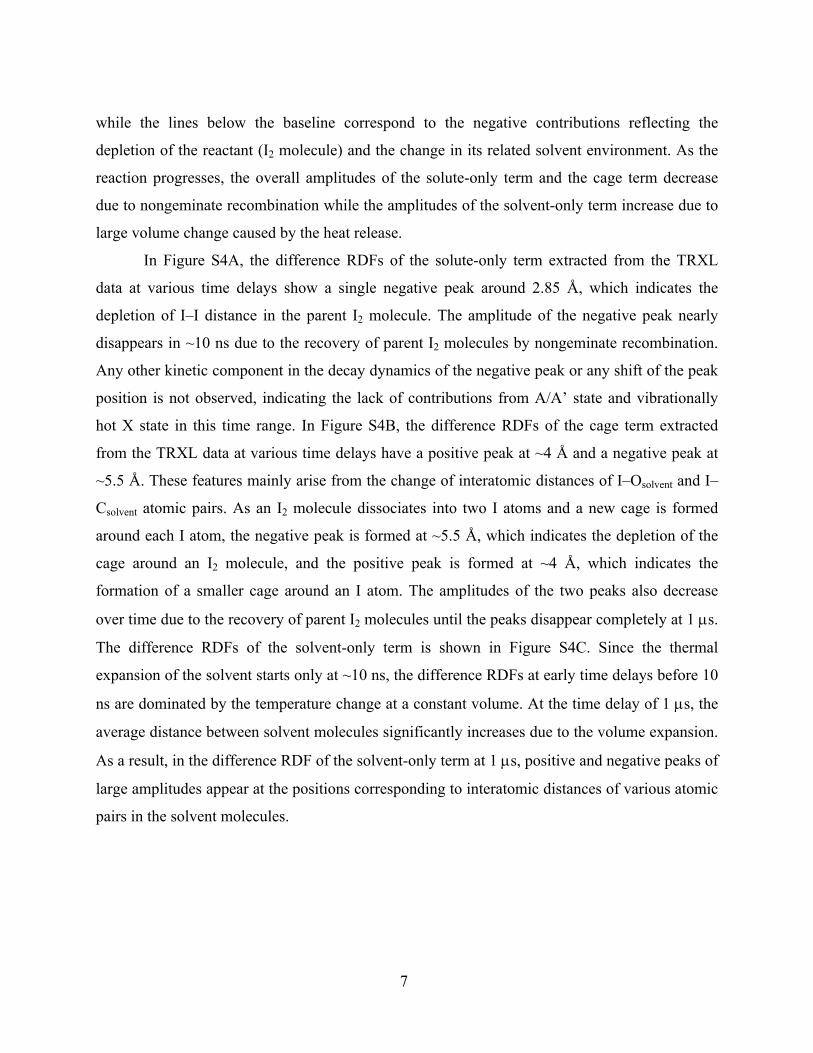
while the lines below the baseline correspond to the negative contributions reflecting the

depletion of the reactant (I2 molecule) and the change in its related solvent environment. As the

reaction progresses, the overall amplitudes of the solute-only term and the cage term decrease

due to nongeminate recombination while the amplitudes of the solvent-only term increase due to

large volume change caused by the heat release.

In Figure S4A, the difference RDFs of the solute-only term extracted from the TRXL

data at various time delays show a single negative peak around 2.85 Å, which indicates the

depletion of I–I distance in the parent I2 molecule. The amplitude of the negative peak nearly

disappears in ~10 ns due to the recovery of parent I2 molecules by nongeminate recombination.

Any other kinetic component in the decay dynamics of the negative peak or any shift of the peak

position is not observed, indicating the lack of contributions from A/A’ state and vibrationally

hot X state in this time range. In Figure S4B, the difference RDFs of the cage term extracted

from the TRXL data at various time delays have a positive peak at ~4 Å and a negative peak at

~5.5 Å. These features mainly arise from the change of interatomic distances of I–Osolvent and I–

Csolvent atomic pairs. As an I2 molecule dissociates into two I atoms and a new cage is formed

around each I atom, the negative peak is formed at ~5.5 Å, which indicates the depletion of the

cage around an I2 molecule, and the positive peak is formed at ~4 Å, which indicates the

formation of a smaller cage around an I atom. The amplitudes of the two peaks also decrease

over time due to the recovery of parent I2 molecules until the peaks disappear completely at 1 s.

The difference RDFs of the solvent-only term is shown in Figure S4C. Since the thermal

expansion of the solvent starts only at ~10 ns, the difference RDFs at early time delays before 10

ns are dominated by the temperature change at a constant volume. At the time delay of 1 s, the

average distance between solvent molecules significantly increases due to the volume expansion.

As a result, in the difference RDF of the solvent-only term at 1 s, positive and negative peaks of

large amplitudes appear at the positions corresponding to interatomic distances of various atomic

pairs in the solvent molecules.

8

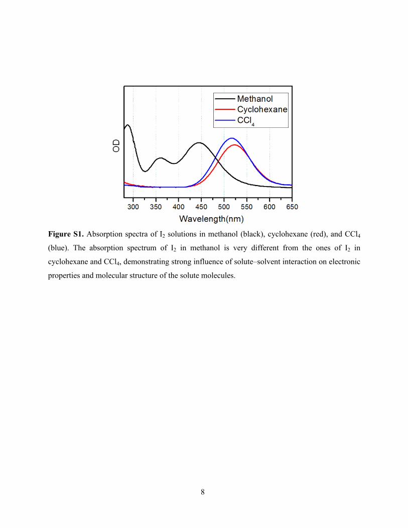
Figure S1. Absorption spectra of I2 solutions in methanol (black), cyclohexane (red), and CCl4

(blue). The absorption spectrum of I2 in methanol is very different from the ones of I2 in

cyclohexane and CCl4, demonstrating strong influence of solute–solvent interaction on electronic

properties and molecular structure of the solute molecules.

9

2 4 6 82 4 6 8

a)Experiment Theory

Diff

eren

ce S

catte

ring

Inte

nsity

, q

S(q

)

q (Å-1)

b)

100 ps

300 ps

700 ps

1 ns

3 ns

7 ns

10 ns

Experiment Theory

Diff

eren

ce R

adia

l Int

ensi

ty, r

S(r

)

1 sx 0.3

100 ps

300 ps

700 ps

1 ns

3 ns

7 ns

10 ns

1 sx 0.3

r (Å)

Figure S2. (a) Time-resolved difference X-ray scattering curves, qΔS(q,t), measured for the

photodissociation of I2 in methanol. Experimental curves at various time delays (black) and their

theoretical fits (red) are shown together. (b) Difference radial distribution functions, rΔS(r,t),

obtained by sine-Fourier transformation of qΔS(q,t) in (a)

10

0.1 1 10 100 10000.40

0.45

0.50

0.55

-0.8

-0.6

-0.4

-0.2

0.0

0.2

0.1 1 10 100 1000

0

1

2

3

4

Con

cent

ratio

n (m

M)

Time (ns)

a)

I

I2

b)

T

(K)

Time (ns)

ρ(kg/m

3)

Temperature Density

Figure S3. (a) Time-dependent concentration changes of transient solute species after

photodissociation of I2 in methanol. The name of each species is indicated above each time trace.

The square points indicate the time delays where the experimental difference scattering curves

were measured. (b) Time-dependent changes of solvent temperature (red) and density (blue) after

photodissociation of I2 in methanol.

11

Figure S4. Reaction mechanism of photodissociation of I2 in methanol.

12

2 4 6 8 2 4 6 8 2 4 6 8r (Å)

O-C + O-OC-C

O-CO-O

c)

rS

(r)

r (Å) r (Å)

rS

(r)

I-I (I2) I-Osolvent I-Csolvent

a) b)

100 ps

300 ps

1 ns

700 ps

3 ns

7 ns

10 ns

1 s

100 ps

300 ps

1 ns

700 ps

3 ns

7 ns

10 ns

1 s

100 ps

300 ps

1 ns

700 ps

3 ns

7 ns

10 ns

1 s

rS

(r)

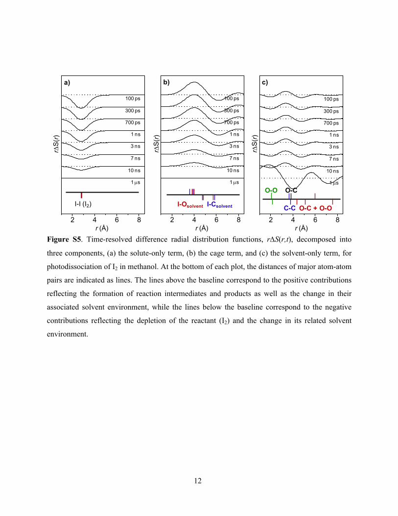
Figure S5. Time-resolved difference radial distribution functions, rS(r,t), decomposed into

three components, (a) the solute-only term, (b) the cage term, and (c) the solvent-only term, for

photodissociation of I2 in methanol. At the bottom of each plot, the distances of major atom-atom

pairs are indicated as lines. The lines above the baseline correspond to the positive contributions

reflecting the formation of reaction intermediates and products as well as the change in their

associated solvent environment, while the lines below the baseline correspond to the negative

contributions reflecting the depletion of the reactant (I2) and the change in its related solvent

environment.

13

2.50 2.55 2.60 2.65 2.70 2.75 2.80 2.85 2.90 2.95

Isolated I2 I2 in methanol

-0.15 -0.10 -0.05 0.00 0.05 0.10 0.15 0.20

Isolated I2 I2 in methanol

Ene

rgy

r (Å)

r-rmin (Å)

Ene

rgy

a)

b)

Figure S6. (a) Potential energy curves of isolated I2 (black) and I2 in methanol (red) calculated

while varying the I–I bond length. For the methanol solution of I2, the solvent molecules were

treated explicitly. The potential energy curve for the isolated I2 has the minimum energy at r =

2.67 Å while the one for I2 in methanol has the minimum energy at r = 2.73 Å. (b) To compare

the widths of the two potential energy curves, we converted the r axis to r – rmin, where rmin =

2.67 Å and 2.73 Å for the isolated I2 and the I2 solution in methanol, respectively. It can be

clearly seen that the potential energy curve for I2 in methanol has a larger width than the one for

the isolated I2, indicating vibrations of larger amplitude and thus weaker I–I bond length of I2 in

methanol.

14

References1. H. Ihee, M. Lorenc, T. K. Kim, Q. Y. Kong, M. Cammarata, J. H. Lee, S. Bratos and M.

Wulff, Science, 2005, 309, 1223-1227.2. J. H. Lee, M. Wulff, S. Bratos, J. Petersen, L. Guerin, J. C. Leicknam, M. Carnmarata, Q.

Kong, J. Kim, K. B. Moller and H. Ihee, J. Am. Chem. Soc., 2013, 135, 3255-3261.3. K. Refson, Comp. Phys. Comm., 2000, 126, 310-329.4. M. Haughney, M. Ferrario and I. R. Mcdonald, J. Phys. Chem., 1987, 91, 4934-4940.5. M. Cammarata, M. Lorenc, T. K. Kim, J. H. Lee, Q. Y. Kong, E. Pontecorvo, M. Lo

Russo, G. Schiro, A. Cupane, M. Wulff and H. Ihee, J. Chem. Phys., 2006, 124.6. S. Jun, J. H. Lee, J. Kim, J. Kim, K. H. Kim, Q. Y. Kong, T. K. Kim, M. Lo Russo, M.

Wulff and H. Ihee, Phys. Chem. Chem. Phys., 2010, 12, 11536-11547.7. J. D. Chai and M. Head-Gordon, Phys. Chem. Chem. Phys., 2008, 10, 6615-6620.8. F. Weigend and A. Baldes, J. Chem. Phys., 2010, 133, 174102.9. E. Cances, B. Mennucci and J. Tomasi, J. Chem. Phys., 1997, 107, 3032-3041.10. A. L. Harris, J. K. Brown and C. B. Harris, Annu. Rev. Phys. Chem., 1988, 39, 341-366.11. N. F. Scherer, D. M. Jonas and G. R. Fleming, J. Chem. Phys., 1993, 99, 153-168.12. M. Wulff, S. Bratos, A. Plech, R. Vuilleumier, F. Mirloup, M. Lorenc, Q. Kong and H.

Ihee, J. Chem. Phys., 2006, 124, 034501.