www.sciencemag.org/cgi/content/full/science.1250770/DC1

Supplementary Materials for

Hydrologic Regulation of Chemical Weathering and the Geologic Carbon Cycle

K. Maher* and C. P. Chamberlain

*Corresponding author. E-mail: kmaher@stanford.edu

Published 13 March 2014 on Science Express DOI: 10.1126/science.1250770

This PDF file includes:

Materials and Methods Supplementary Text Figs. S1 to S8 Table S1 References (33–92)

1

Materials and Methods Derivation of solute production function (equations (1) and (3), main text)

The present work presents a dimensional analysis of global chemical weathering rates and their response to tectonic and climatic changes at the Earth’s surface. At this scale, chemical weathering rates are typically represented in terms of the solute flux exiting a catchment, and are calculated as the product of the riverine concentration and runoff. To model weathering fluxes, it thus is necessary to first determine the solute concentration. The concentration depends on the amount of time that water spends in the subsurface, or the fluid travel time, because mineral dissolution is governed by kinetic reactions (5, 16, 33, 34). When the water exits the catchment, the concentration of the river records the amount of dissolution. However, catchments are characterized by a distribution of fluid travel times. Each flow path within the distribution has a unique travel time and concentration such that the final concentration in the river is weighted by the travel time distribution (Fig. S1). This mixing effect must be accounted for in describing the concentration.

To explain how concentrations are linked to the fluid travel time distributions, we first review a one-dimensional model for solute production as a function of fluid travel time along a single flow path. This approach was previously applied to soils (34) and small catchments (16). To obtain equation (3) (main text), which accounts for the distribution of fluid travel times, we extend this earlier approach to three-dimensions using a stochastic representation of travel times pervasive in catchment hydrology (e.g., reviews by 35, 36). Subsequently, we explain how the dissolution kinetics, that control the rate of increase in the concentration at a given flow rate, are factored into equation (3) through constitutive relationships (e.g., equations (1) and (2) main text).

The solute production model represented by equation (3) is not aimed at predicting seasonal or storm-driven concentration-discharge relationships, but rather long-term variations in physical processes that impact the global distribution of Dw and runoff values.

The basis for the solute production equation is the analytical solution to the advection-reaction equation for heterogeneous irreversible reactions where the concentration of a dissolving solute (c [µmol/L]) along a flow path (x) is a function of the flow rate or runoff (q [m/yr]), the effective porosity (φ), the initial concentration (co), the equilibrium concentration (ceq) and the net dissolution rate (Rn [µmol/L/yr])(16):

c(x) = c0 exp−Rnφxτqceq

⎛

⎝⎜⎞

⎠⎟+ ceq 1− exp

−Rnφxτqceq

⎛

⎝⎜⎞

⎠⎟⎛

⎝⎜

⎞

⎠⎟ (S1)

The equation predicts an increase in solute concentration until thermodynamic equilibrium (ceq) is reached (Fig. S1). The limit is assumed to reflect equilibrium between the secondary and primary mineral assemblage such that there is no additional increase in concentration with increasing distance. The scaling factor, τ = e2, allows for the concentration to reach 99.9% of ceq when the travel time equals the equilibrium time. Both ceq and Rn are a function of temperature, composition (including mineral, gasses and liquid saturation) and mineral concentrations (37) and a sensitivity analysis is provided in ref. (16), with further discussion in subsequent sections. The theoretical maximum solute flux is achieved when the water spends sufficient time in the subsurface to reach equilibrium among the primary and secondary minerals (Wmax = qceq).

2

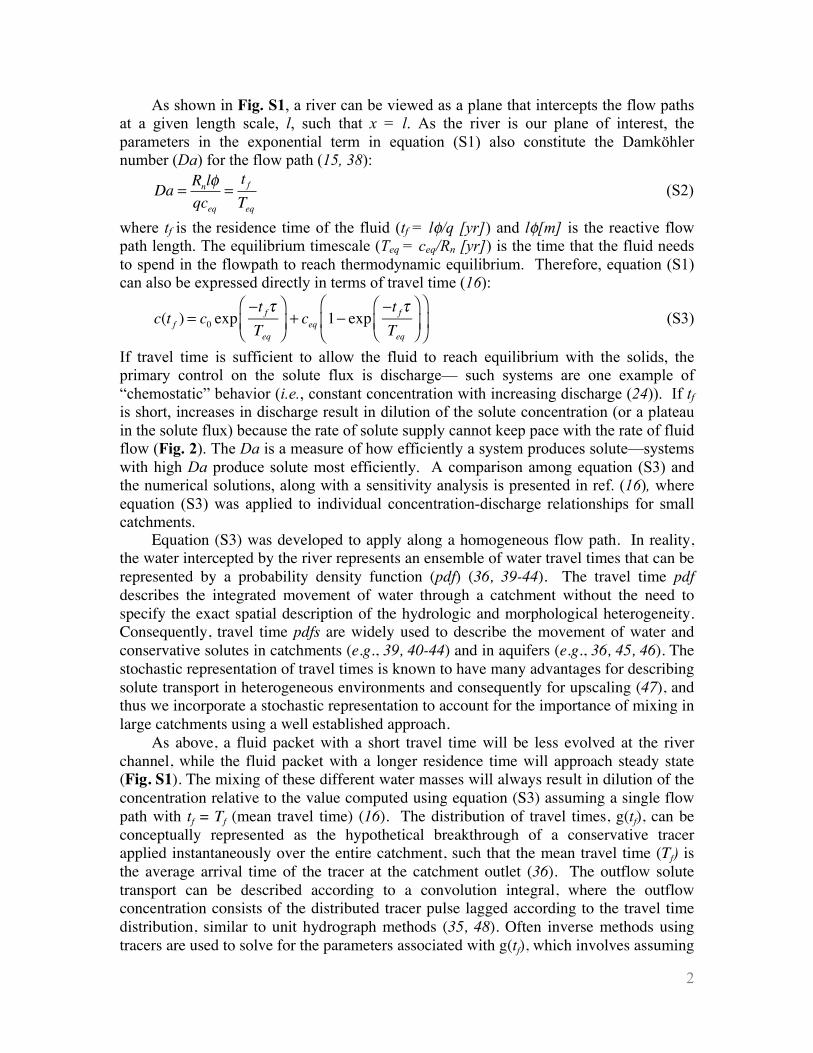
As shown in Fig. S1, a river can be viewed as a plane that intercepts the flow paths at a given length scale, l, such that x = l. As the river is our plane of interest, the parameters in the exponential term in equation (S1) also constitute the Damköhler number (Da) for the flow path (15, 38):

Da = Rnlφqceq

=t fTeq

(S2)

where tf is the residence time of the fluid (tf = lφ/q [yr]) and lφ[m] is the reactive flow path length. The equilibrium timescale (Teq = ceq/Rn [yr]) is the time that the fluid needs to spend in the flowpath to reach thermodynamic equilibrium.

Therefore, equation (S1)

can also be expressed directly in terms of travel time (16):

c(t f ) = c0 exp−t fτTeq

⎛

⎝⎜⎞

⎠⎟+ ceq 1− exp

−t fτTeq

⎛

⎝⎜⎞

⎠⎟⎛

⎝⎜

⎞

⎠⎟ (S3)

If travel time is sufficient to allow the fluid to reach equilibrium with the solids, the primary control on the solute flux is discharge— such systems are one example of “chemostatic” behavior (i.e., constant concentration with increasing discharge (24)). If tf is short, increases in discharge result in dilution of the solute concentration (or a plateau in the solute flux) because the rate of solute supply cannot keep pace with the rate of fluid flow (Fig. 2). The Da is a measure of how efficiently a system produces solute—systems with high Da produce solute most efficiently. A comparison among equation (S3) and the numerical solutions, along with a sensitivity analysis is presented in ref. (16), where equation (S3) was applied to individual concentration-discharge relationships for small catchments.

Equation (S3) was developed to apply along a homogeneous flow path. In reality, the water intercepted by the river represents an ensemble of water travel times that can be represented by a probability density function (pdf) (36, 39-44). The travel time pdf describes the integrated movement of water through a catchment without the need to specify the exact spatial description of the hydrologic and morphological heterogeneity. Consequently, travel time pdfs are widely used to describe the movement of water and conservative solutes in catchments (e.g., 39, 40-44) and in aquifers (e.g., 36, 45, 46). The stochastic representation of travel times is known to have many advantages for describing solute transport in heterogeneous environments and consequently for upscaling (47), and thus we incorporate a stochastic representation to account for the importance of mixing in large catchments using a well established approach.

As above, a fluid packet with a short travel time will be less evolved at the river channel, while the fluid packet with a longer residence time will approach steady state (Fig. S1). The mixing of these different water masses will always result in dilution of the concentration relative to the value computed using equation (S3) assuming a single flow path with tf = Tf (mean travel time) (16). The distribution of travel times, g(tf), can be conceptually represented as the hypothetical breakthrough of a conservative tracer applied instantaneously over the entire catchment, such that the mean travel time (Tf) is the average arrival time of the tracer at the catchment outlet (36). The outflow solute transport can be described according to a convolution integral, where the outflow concentration consists of the distributed tracer pulse lagged according to the travel time distribution, similar to unit hydrograph methods (35, 48). Often inverse methods using tracers are used to solve for the parameters associated with g(tf), which involves assuming

3

a particular form of the pdf, as the true distribution is unknown. The commonly assumed forms of the pdf include piston flow (which would be equivalent to equation (S3)) and exponential, gamma or beta distributions. For a reactive solute, distributions skewed towards shorter travel times (e.g., gamma distribution) tend to result in greater dilution but the same general behavior as equation (S3) (see figure 7, ref. (16)). Below we develop equations to quantify this effect.

To account for heterogeneity in travel times, we incorporate a mean travel time (Tf) approximation assuming an exponential distribution (36, 40):

g(t f ) =1Tf

exp −t fTf

⎛

⎝⎜⎞

⎠⎟, (S4)

with mean, Tf, defined as the first moment of g(tf):

Tf = t f1Tf0

∞

∫ exp−t fTf

⎛

⎝⎜⎞

⎠⎟dt f . (S5)

To calculate the mean concentration (C) for Tf due to mixing of fluids from different flow paths we integrate the convolution integral for c(tf) and g(tf) as one would for a conservative tracer:

C(Tf ) = c(t f )1Tf0

∞

∫ exp−t fTf

⎛

⎝⎜⎞

⎠⎟dt f . (S6)

The function describing the distributed solute production, c(tf), is a function of the time that the fluid contacts the minerals according to equation (S3) above, which is also the solution to the equation for the change in concentration as a function of tf:

dcdt

= Rn 1−cceq

⎛

⎝⎜⎞

⎠⎟ . (S7)

We apply equation (S3) to the convolution integral and combine terms to yield:

C(Tf ) = ceq −ceqTf

exp −t fτTeq

+ 1Tf

⎛

⎝⎜⎞

⎠⎟⎛

⎝⎜

⎞

⎠⎟

0

∞

∫ + c0Tf

exp −t fτTeq

+ 1Tf

⎛

⎝⎜⎞

⎠⎟⎛

⎝⎜

⎞

⎠⎟ dt f (S8)

which can readily be integrated to yield the equation for the mean concentration, C, weighted by the travel time distribution as presented in equation (3) in the main text. We further distinguish concentrations (C0, Ceq) and length scales (Lφ) between the 1-D (lowercase) and effective 3-D equation (uppercase), as the values used for a catchment may not be the same as for a single one-dimensional flowpath.

The Da coefficient can then be used in the resulting solution to equation (S8). If the effective Da is now = Tf/Teq, then discharge (q) can be factored out to obtain the dimensional coefficient, Dw, of equation (1) (main text):

Dw[m / yr] = LφTeq

(S9)

When this equation is inserted into the solution to equation (S8), the result is:

C = C01+τDw / q

+CeqτDw / q1+τDw / q

. (S10)

This is the solute production equation represented by equation (3) (main text). The Da (=Dw/q) is now described in terms of Tf, and τ = e2. For modeling SiO2(aq) variations, we

4

also assume that Co is zero. The stochastic treatment of travel times embedded in equation (S10)/equation (3) (main text), which is widely used in catchment and groundwater solute transport, effectively extends the equation for C to three-dimensions making it useful for predicting solute production in a catchment, without deterministically assigning heterogeneity. Although other functions for g(t) have been proposed, the exponential is widely used, and we note that given the typical noise and poor temporal resolution in concentration-discharge data for solutes, it is often difficult to decipher the subtle differences among distributions (36).

Fig. S1 presents a conceptual model comparing equation (S3) to equation (S10) (equation (3), main text) demonstrating that for the same value of tf (or flow path length, l) and Tf (or mean flow path length, L), the concentration is lower using equation (S10) because of the dilution imparted by the fraction of shorter flow paths that experience less solute production. In our model, the concentrations are weighted by the travel time distribution, which in turn imposes a distribution of fluxes based on the assumed mean value of Lφ. The solute production model is not aimed at predicting seasonal concentration-discharge relationships, but rather long-term (ca. >1 kyr) variations in physical processes that impact the global distribution of Dw and runoff values. Nevertheless, it can be applied to interpret seasonal discharge-concentration variations as shown in ref. (16), although the approach warrants more detailed investigation at seasonal time scales because of the likely transience in the travel time pdf.

Derivation of reaction rate formulation and fw (equation (2), main text) In the conceptual model above, Dw describes the efficiency of solute production as a

function of the dissolution kinetics (relative to Lφ). Thus, concentrations will increase more rapidly if the reaction rate is higher (see equation (S7)). To model concentration therefore requires the hydrologic component outlined above, and a description of how reaction rates change across different weathering environments. At the global scale, a key variable is erosion rate because erosion removes the previously weathered material, which in turn drives the conversion of fresh bedrock to regolith bringing fresh minerals into the weathering zone (19, 25, 26, 49-52). The effect of increasing reaction rates is shown schematically in Fig. 1 (main text), where the solid black line represents the solute production for rapid kinetics (short Teq and residence time of mineral in the weathering zone, Ts) and the stippled lines are effectively contours of decreasing reaction rates (i.e., longer Teq and Ts).

The connection between soil production and mineral dissolution kinetics is driven primarily by two factors: (1) the total surface area of dissolving mineral, which determines the supply rate of ions to solution, and (2) the fluid to rock ratio, which determines the amount of surface area per volume of fluid. A third factor that impacts the dissolution rate is the approach to equilibrium, which is already included in the model as Ceq. The maximum reaction rate occurs when the concentration of mineral in the soil (or weathering zone) equals that of the fresh bedrock, and is defined here as:

Rn,max[µmol / L / yr]= ρsf keff AXr (S11) where ρsf [g/L] is mass of solid to volume of fluid ratio, which is a function of the porosity and is calculated as ρ/φ, where ρ is the solid density and ρf the fluid density), keff [mol/m2/yr] is the dissolution rate constant (or the net dissolution rate if a secondary mineral is precipitating), A [m2/g] is the specific surface area and Xr [g/g] is the

5

concentration of reactive mineral in a soil composed entirely of fresh bedrock (see Table S1 for a list of parameter definitions and values). The product ρsfAXr [m2/L] reflects the total surface area per volume of fluid, while keff [mol/m2/yr] is an intrinsic constant that is specific to a given mineral. We assume that the primary influence of soil production is to alter ρsfAXr by controlling the ratio of the concentration of the mineral in the soil, Xs [g/g] to Xr, which we define as fw (=Xs/Xr). As soil production rates decrease, the residence time of material in the weathering zone increases and fw approaches zero. The Rn,max is reduced according to the value of fw:

Rn = Rn,max fw = ρsf keff AXr fw (S12) Soil production, which is linked to erosion, is not the only control on fw. In the absence of erosion, as a soil ages it also becomes depleted in fresh minerals such that fw decreases with increasing “soil age” (20, 25, 53, 54). Effectively fw depends on the age of the material in the weathering zone, requiring a second set of equations that predict fw across a broad range of erosion rates, from zero (e.g., glacial deposits, floodplains and river terraces) to the very high rates associated with active mountain belts (e.g., hillslopes).

Most models for fw (or for other similar parameters that reflect the amount of fresh mineral) assume geomorphic steady state where soil thickness is constant over time because the fresh mineral supplied to the weathering zone at flux (P) is balanced by erosion (E) and weathering (W) (e.g., refs. (27, 49, 50, 55)). The total denudation rate (D) is the sum of the E and W. Under non-steady state conditions the top of the weathering zone becomes depleted in fresh mineral and weathering occurs deeper in the profile. These conditions of “supply-limitation” can result in highly weathered profiles with very low fw, and may be typical of cratons and other geomorphic provinces with low rates of sediment supply (25). In order to expand the range of conditions over which fw can be evaluated, we derive a new set of equations that do not require a steady state assumption and then simplify them to obtain the scaling relationship between fw and soil residence time (Ts) of equation (2) (main text).

As above, the change in the mass of the soil reservoir and the concentration of mineral within that reservoir over time are a function of the balance between P (supply) and E and W (removal) according to the following equation:

M dXs

dt+ Xs

dMdt

= PXr − EXs −Mmkeff AXs

(S13)

where M is the total mass in the weathering zone and mkeffA [yr-1] is the product of the molar mass (m [g/mol]), the rate constant (keff [mol/m2/yr]) and the specific surface area (A[m2/g]). This equation is similar to previous formulations (e.g., ref. (49), except that the left hand side has been expanded to account for the change in both mass and mineral concentration. By solving the mass balance relationship for dM/dt only in terms of P-D, M can be expressed in terms of the initial mass (M0) plus the additional change in mass: (P-D)t:

M (t) = M 0 + (P − D)t (S14) This simple linear relationship assumes no first order dependence of P, E or W on M. Imposing such a dependence (i.e., W = kM) would create a negative feedback between weathering and M that is physically unrealistic as it would force soil thickness to converge on a constant value at a given P. However, other descriptions of dM/dt and M can be used. Mass (M) can subsequently be replaced by soil residence time (Ts) in the

6

final equation, at which point any model for soil residence time can be employed (see supplemental text S1). The above relationship for M is substituted into equation (S13):

M 0 + (P − D)t[ ]dXs

dt+ Xs (P − D) = PXr − EXs −mkeff AXs M 0 + (P − D)t[ ] . (S15)

After rearranging, the final equation predicts a decrease in fw with time: dXs

dt= P(Xr − Xs )M 0 + (P − D)t

−mkeff AXs

. (S16)

This equation can be solved both numerically for Xs/Xr (i.e., fw) and evaluated using reactive transport approaches as discussed below (Fig. S2). A special case of equation (S12) would correspond to quasi-steady state mineral concentration (i.e., dXs/dt à 0). When the left-hand side of equation (S16) is set to zero, the residual fresh mineral content is inversely related to the ratio of the weathering rate to the soil production rate, times the mass of the material:

Xs

Xr

= 1

1+mkeff AP

M 0 + (P − D)t( ). (S17)

To further simplify, we note that if (MO +(P-D)t) is equal to the mass of the column, then the soil residence time or “soil age” (Ts) is the ratio M/P, or the average age of the soil, if known. The following simplified statement relates the mass of fresh mineral as the weathering fraction (fw) (i.e., Xs/Xr as per equation (2), main text) to the inverse of the product of the reaction rate and the “soil age” (equation (2), main text).

fw =Xs

Xr

= 11+ mkeff A( )Ts (S18)

Equation (S18) captures the 1/Ts dependence of reaction rates observed in studies of chronosequences (i.e., soils of different ages) developed on alluvial material and in marine sediments (34, 56, 57) (Fig. S2). This formulation differs from previous models that consider the supply of fresh mineral to the soil zone via erosion (49, 50) because it does not impose steady-state soil thickness. However, similar to previous models it does predict a decrease in Xs/Xr with increasing soil age or residence time, resulting in a decrease in Rn via equation (S12); (Fig. S2). As the purpose of equation (S18) is to scale the equilibrium times associated with chemical weathering fluxes as a function of denudation rate, this simple relationship is appropriate for global solute fluxes, while more detailed models may be required for hillslope-scale studies. The parameterization of equation (S18), along with a comparison to numerical solutions of equation (S16) are presented in the following section on model parameterization, while the consequences of different Ts formulations are described in the supplemental text S1.

When fw is thus incorporated into Dw, increasing soil production or decreasing Ts increases the Dw resulting in more efficient solute production according to equation (1)(main text):

Dw[m / yr]= LφRnCeq

=LφRn,max fw

Ceq

(S19)

The Dw is then used in equation (3) to compute solute concentrations and fluxes (parameter definitions and values are also provided in Table S1).

7

In the application of equation (S18) to equation (3), mixing among flowpaths with different extents of reaction progress is accounted for, but compositional heterogeneity (i.e. variation in fw) across flow paths is not explicitly accounted for. This is justified because mixing due to physical heterogeneity has been shown to overprint compositional heterogeneity when fluid travel times are sufficiently long (58, 59) (i.e. fluid composition is the same for both homogeneous and heterogeneous mineral distributions). Thus, the assumption of an average fw is reasonable for large systems where mixing is efficient. However, even if there was a systematic relationship between fw and flowpath length, concentrations would still increase towards equilibrium and thus the shape of the concentration-travel time curve might be altered from that of Fig. 1, but would maintain the same general behavior. In practice, such differences between concentration curves may be indistinguishable given the variability in actual data (16, 36). In summary, although compositional variations around the average fw are certainly likely, mixing should result in fluids that reflect the average value of the solid. Evaluation of equations (1) - (3) and associated parameters using numerical methods

In order to evaluate the application of equations (1-3) (main text), including the change in the mineral abundance (fw) and the thermodynamic limit (Ceq), we use two approaches: (1) A multi-component reactive transport model (RTM), CrunchFlow2007. The RTM

uses the simulation conditions presented in ref. (16), including experimentally determined rate constants and rate laws. These simulations are expanded here to include variable erosion rates from 0 to 5 mm/yr and flow rates from 0.1 to 3 m/yr resulting in 80 numerical realizations. The RTM results are only used to estimate the maximum rate in equations (1)-(3) (main text) and to evaluate the scaling relationship between fw and Ts, along with a comparison to two data sets for large rivers are presented in the supplementary text. Figs. 2 and 3 (main text) are independent of the RTM results.

(2) Equation (S16) was numerically integrated using a fourth-order Runge-Kutta routine implemented in MATLAB R2013a and compared to the results of the RTM approach and equation (2) (main text) (Fig. S2).

Model parameterization and calculations Ceq: In our application of the model to calculate global Dw contours in Figs. 2 and 3 (main text), the only parameter we assume is the global equilibrium concentration (Ceq) of 375 µmol/L, which is based on the maximum SiO2(aq) concentrations for global rivers (8) (95% confidence interval (60)) and is compared to theoretical calculations in Fig. S3, although the approach could be adapted to consider alkalinity or other cation fluxes (Table S1). Fluxes of SiO2(aq) have been used as a silicate weathering proxy in previous studies (49, 61) and are used here to reduce the dependence on the base cation stoichiometry of the rocks and uncertainty associated with correction of river data for carbonate or evaporite weathering. For the data sets evaluated here the correlation between SiO2(aq) and silicate cation denudation rate is reasonable (R2=0.50 (8), n= 70; R2=0.79 (62), n=20;). The Ceq represents the endpoint for the metastable equilibrium between a dissolving (feldspar) and precipitating mineral (clay) and as such it depends on

8

the activities of ions in solution, and in particular on pH. Our estimate, which is meant to represent a conservative global maximum value, clearly does not capture the individual value for each river. However, our calculations (Fig. S3) and phase equilibrium considerations (63) show that it is unlikely to be much lower: more crystalline secondary minerals (e.g., kaolinite) tend to increase Ceq, while variations between plagioclase(An20) and pure albite or K-spar generally result in <25% increase for the same conditions. Basaltic lithologies may also have greater Ceq values (as discussed in supplementary text S3). However, lithologic variations are more likely to result in greater variations in Rn because this term also depends on mineral volume and surface area. As a result, for calculating relative changes in weathering fluxes, the assumed value of Ceq is less important than the change in runoff or Ts, which can both vary by several orders of magnitude. A sensitivity analysis regarding the consequences of selecting a single global equilibrium endpoint is presented in Supplementary Text S5 and Fig. S8. Rn,max and fw: To compute the effective reaction rate (Rn), the Rn,max value is scaled according to fw, which is a function of Ts. The Rn, max represents the theoretical maximum for a column of fresh material (fw = 1) and is computed from the RTM simulations (using established kinetic rate constants) to be 1085 µmol SiO2/L/yr (see table S1 for all parameters, and for values of other components of interest, such as alkalinity). The mkeffA is similarly computed to be 8.5 x 10-5 g/g/yr while Ts is treated as a variable. Although these values require assumptions that may not be applicable over all systems, for the present study it is the contours of Dw which do not depend on the assumed values, that represent the key feature of the model that predicts how weathering rates per unit area land surface vary in response to climatic and tectonic perturbations.

A comparison of the results from the RTM simulations, the numerical solution of equation (S16) and the scaling relationship of equation (S18) (equation (2), main text) is shown in Fig. S2. We calculate Ts as M/P and set the mass equal to Mo+(P-E)t in solving equation (S16) numerically. The latter simplification turns out to be of little consequence as indicated by the agreement between the RTM model and the solution to equation (S18). The points from RTM simulations correspond to both steady and non-steady geomorphic conditions as a function of soil residence time. Mass is calculated as the depth of weathering. The two numerical solutions (RTM and numerical solution to equation (S16)) and the scaling argument (equation (2) main text) show reasonable agreement over the four orders of magnitude in soil residence times given that fw changes non-linearly with Ts. This result is consistent with the idea of supply-limitation (25, 27, 62) where the increasing importance of mineral supply is apparent in the increase in slope of the model lines for Ts > 1 kyr in Fig. S2. The reactive transport simulations also show more scatter at low erosion rate/low fw because of the increasing importance of flow rate, which controls the weathering advance rate. More elaborate relationships among flow rate, erosion rate, mineral kinetics and soil residence time could be substituted for equation (2), but we conclude from this comparison that the scaling model is appropriate for large variations in Ts.

The general agreement between the scaling relationship and the two models of varying complexity is reasonable, and supports the use of the fw parameter to scale the reaction times as proposed in equation (2). Although this approach is simplified to extend over a large range of conditions, it is generally consistent with other models and field

9

studies that have examined soil mineralogy during weathering (cf. 19, 20) and captures the apparent decrease in weathering rates with increasing soil age (cf. 34, 56). Dw: To compute the curves in Figs. 1-3 we calculate the maximum and minimum Dw coefficients using the concentration and discharge data (8) and the Ceq value above. We show the contours of Dw, which do not depend on the chosen values of Rn, fw or Ts, to illustrate how systems respond in a relative sense to climatic and tectonic variations. Then, using the range of Dw coefficients we partition the Dw coefficients between the Lφ and Teq assuming Rn,max = 1085 µmol/L/yr. For example, a Dw of 0.3 (global maximum) requires an Lφ of 0.1 m for Ts of < 1 kyr. If we hold Lφ constant, this results in a soil residence time of 1 Myr at Dw = 0.003 (~global minimum). Values of Ts between 5000-200 kyr in regions of low uplift (10-3 mm/yr to 10-2 mm/yr) and between 200 kyr and 0.2 kyr in regions of high uplift (10-2 to 10 mm/yr) are typical of large river systems (49). In Figs. 2-3, reactive length scale (Lφ) is held constant consistent with the suggestion of minimal variation in L (27), but in reality this parameter is likely to cause variations in Dw. This assumption is further discussed in Supplementary Text S1. Importantly, the global Dw contours are independent of these assumptions—their purpose is to provide physical context. Ultimately, because the Dw is the ratio Lφ/Teq, relative changes in this ratio drive global shifts in solute fluxes and therefore parameters chosen for Ceq, Rn, keff, Lφ and Ts are not critical for predicting relative changes in solute fluxes shown in Fig. 3. A sensitivity analysis is presented in supplementary text S4.

All parameters are not perfectly known and key assumptions (such as the stochastic representation of travel time) require further evaluation. To further test this approach will require independently calculating Dw coefficients for the large river systems and comparing them to Dw coefficients and Ceq values calculated from concentration and discharge data. This will require abundant spatially and temporally resolved concentration-discharge and erosion rate data from large rivers to support robust inverse methods. At present, sufficient data for large rivers is not available.

Supplementary Text S.1 Model evaluation I: Relationship between erosion rate, water flux and solute flux

The final parameters for the solute production model consist of the weathering Dw coefficient, the equilibrium concentration and the runoff. The Dw coefficient reflects the ratio between the reactive flowpath length (Lφ), which determines Tf at a given flux, and the timescale associated with the chemical reactions, and thus higher Dw values indicate a more rapid approach to the thermodynamic limit at a given Tf because the flowpath is more reactive, Lφ is large, or both. The consequences of variations in Rd, Ts and Ceq and the corresponding Dw values are shown in Fig. S4. The Ceq becomes increasingly important to the concentration at long fluid travel times, while the importance of the reaction rate decreases at long fluid travel times.

The Dw is also linked to surface age and/or soil production rate through fw as demonstrated in Fig. S2. Thus, to estimate solute production using equations (1)-(3) requires either knowledge of (a) soil residence time as in Figs. 1, S2, etc. or (b) soil production rate and a constitutive relationship for regolith thickness (h). An additional consideration surrounds whether (1) L is equal to h, implying that mean fluid travel time

10

is also linked to regolith thickness, or (2) whether L varies independent of h. There is currently insufficient data to determine whether travel time is directly linked to regolith thickness, although most studies assume that weathering predominantly occurs within the region defined by h. However, in large basins solute exchange with floodplains/hyporheic zones and groundwater inputs may result in decoupling of h and L, where the latter defines Tf. Below we assess the consequences of these assumptions on predicted weathering fluxes.

We assume below geomorphic steady state such that P is correlated with E. There are numerous models proposed to link erosion rate to h or Ts. A simple empirical relationship for h as a function of E is used here to illustrate how the coupling between solute production and erosion is implemented through Dw and q, and to provide a comparison to previous literature approaches as a means to evaluate the scaling of the model. We then further assess the implications of assuming L= h.

The relationship between E and h (50) applied here was used previously to relate chemical weathering fluxes to erosion rates:

h[km]= ln(E[t / km2 / yr] /104.01[t / km2 / yr]2300[km−1]

(S20)

From this, soil residence time, Ts [yr-] (50) is: Ts[yr]= ρ[t / km3]h[km] / E[t / km2 / yr] (S21)

where the soil density, ρ, is assumed to be 1.3 x 109 t/km3 (50). Additionally, we compute the model of ref. (50) (GM2009 hereafter), which also links erosion rates to chemical weathering fluxes, using the the published parameters (note that the value for the empirical constant kh = 104.01 t/km2/yr) in equation (S20) is the value used in the GM2009 calculations, although a different value is provided in the text, E. Gabet, personal communication). A functional difference between the two models is that the solute production model (equations 1-3, main text) includes the dependence on fluid travel time.

We consider two scenarios: scenario 1 where L is independent of h and scenario 2 where L = h. For scenario 1, L is set to 2 m in calculation of Dw. For scenario 2, because Tf is represented here by a pdf, setting L= h assigns an exponential distribution to regolith thickness with a mean h. We use the same porosity (0.52) between both scenarios as defined by the ρ assumed in GM2009. To convert to chemical weathering fluxes, we assume a value for m of 270 g/mol and a stoichiometric ratio of 1.67 mol Si/mol plagioclase, which accounts for the consumption of Si by halloysite. Both models are compared to the data of ref. (62), which was also used in GM2009 (where the data at high erosion rate was corrected for climate in their comparison). Here we show only original data. This ensemble constitutes data from small catchments (< 103 km2) at high erosion rates, and larger catchments from stable cratonic settings. The catchment data of ref. (62) and GM2009 model were not used in the model development, and thus represent an independent means of evaluating the solute production model.

Fig. S5 presents the comparison between the model of GM2009 and the solute production model for scenarios (1) and (2) at a range of q values. For scenario 1, the solute production model predicts plateaus in chemical weathering fluxes associated with thermodynamic limitation. This occurs because although h approaches zero at high erosion rates, by decoupling L this scenario effectively assumes that the water contacts fresh mineral beyond the weathering zone, with a composition (fw) that is still determined

11

by Ts. This scenario may be reasonable for large basins where eroded material is contained in downstream floodplains and Tf can reach tens of years (40).

For scenario 2, both models predict a similar maximum in weathering rates at a particular soil thickness, although the maximums occur at different soil thicknesses: in the solute production model this maximum occurs where fluid travel times are balanced by high fw, allowing for the Ceq to be reached. The plateau captures the apparent plateau in solute fluxes at high erosion rates (often called “kinetically-limited” weathering). At very high erosion rates, weathering rates decline because of the decrease in travel time (i.e., Ceq can longer be obtained). Although the “humped” behavior of both models is generally similar, another clear difference between the models is the variation in flux at different runoff values predicted by the solute production model. The data of ref. (62) is also color scaled according to runoff for comparison to the solute production contours. Although the solute production model does not perfectly match the runoff values, the general agreement is reasonable given that no additional parameter fitting was done here in order to provide a direct assessment of the model behavior. The agreement between the model and measured chemical weathering fluxes, erosional fluxes and runoff is better for the large rivers (Fig. S6).

Although we cannot resolve which scenario is most applicable, we suggest that scenario 2 may be more applicable to hillslopes and small catchments, while perhaps scenario 1 is more likely to apply to large basins. The solute production model also directly includes a dependence on runoff, which is shown here to be important.

A key conclusion from this comparison is that if h also controls Tf (scenario 1) that the solute production model captures the “humped” behavior of solute fluxes predicted by other models, even those derived at the scale of soil profile (e.g., refs. (19, 64). The comparison also demonstrates that the model passes a critical scaling test by matching observed relationships from soils/hillslopes and small catchments.

S.2 Model evaluation II: scaling and comparative analysis

The basin-scale solute production model builds primarily on observations and paradigms developed at the hillslope to small catchment scale, respectively. If the dominant processes change with scale, then the use of the effective parameters is unreasonable. Our analysis is in part a dimensional technique based on the Da, wherein the utility rests in the concept of dynamic similarity. In upscaling the model from equation (S3), distribution is accomplished stochastically through the travel time pdf, which is then aggregated to provide a single value, Tf. This stochastic approach is advantageous in that although the detailed pattern is not known, the distribution can be inferred. We did not upscale the reaction rate parameters (aside from the scaling function, fw) because of the agreement between the RTM model predictions and the global river data (Figs. S4 and S6).

A critical question is thus model performance at the scale of interest, which is challenging as some of the key data has not been collected. Below we provide several lines of evidence to suggest that the model is scale-appropriate. We demonstrate that: (1) the solute production model incorporates key features of weathering processes generally observed at smaller scales, and hence the derived model produces reasonable agreement with observations at smaller scales, a critical scaling test (i.e., downward approach); and

12

(2) when compared to data sets not employed for calibration, the model reproduces the key features of the data.

(1) Model-theory intercomparison: In developing the solute production model, three key features of weathering processes that have emerged from decades of detailed study were included. These three key features are: (1) Solute concentrations must increase along a flow path until thermodynamic equilibrium is achieved (53, 54, 63, 65-72). This is shown conceptually in Fig. 1 (main text). (2) Some rivers show relatively constant concentration with discharge while others do not, indicating that the efficiency of dilution and thermodynamic equilibrium varies in importance from catchment to catchment (16, 24, 73-75). The importance of dilution is shown in Fig. 2A (main text), where rivers with high Dw values show relatively less dilution at high runoff compared to rivers with low Dw. (3) The total amount of fresh mineral in the weathering zone is a function of the erosion rate, and this in turn impacts the weathering rate (19, 25, 26, 49-52). The ultimate response to increased weathering kinetics is to impact the rate of approach to thermodynamic equilibrium (20, 34, 54, 70). This response is shown clearly in Figs. 1, 2, S3, S5, where higher Dw values correspond to a more rapid increase in solute concentrations along a flow path. Our model mathematically reproduces these key observations, which originally formed the basis for the derivation, but does not imply that it has predictive power.

(2) Model-data intercomparison: As shown in the previous section and Fig. S5, the solute production function produces results comparable to the model of GM2009 under certain conditions. A second test of the model is provided in Fig. S6A, where we show the results from the RTM simulations, and the global dataset of ref. (8) relative to the model predictions from scenario 2 (i.e., assuming h = L as in Fig. S5E)). We draw this comparison for several reasons. First, the agreement with measured runoff is considerably improved when the model is compared to larger rivers, and shows that the contours reflecting different runoff values are capturing both the total denudation rate and the effect of increased runoff on the solute flux, despite the independent assignment of a relationship between soil residence time and erosion rate. Second, the RTM simulations represent geomorphic steady-state conditions associated with thermodynamic limitation, which is consistent with the “hump” in the solute production model. The RTM realizations and solute production descriptions here are independent of one another, aside from the net reaction rate term.

Fig. S6B shows the relationship between calculated riverine Dw values and weathering fluxes. As the Dw is calculated from the measured concentrations and runoff using equation (3) main text, the two are not entirely independent. However, the strength of the relationship shows the ultimate utility of the Dw for calculating weathering flux, especially if Dw can be independently evaluated. The plateaus in SiO2(aq) flux with increasing Dw represent the humps or plateaus in Fig. S6A and indicate the importance of thermodynamic limitation. This decoupling of Dw and weathering flux occurs because SiO2(aq) flux becomes independent of Dw and more dependent on runoff and Ceq as the thermodynamic limit is approached. The distribution off points along the plateaus indicates the importance of both Ceq and dilution.

Fig. S6C shows an alternative test of the solute production model relative to the global data set. Here, Dw values are calculated for each river from equation (3) (main text) using the Ceq value and measured concentrations and discharge, and compared to

13

erosion rates represented by total suspended sediment (TSS) flux (8) and from a combination of TSS fluxes and cosmogenic nuclides (62). The model relationships predicted from scenarios 1 and 2 (Fig. S5) are also shown representing the Dw imposed by equations (S18) and (S19). First, because the calculated Dw values and the TSS fluxes are calculated entirely independent of one another, the observed correlation supports the premise that higher Dw values reflect more efficient solute generation associated with more reactive flowpaths. However, the correlation is weak, most likely because the relationship between erosion rate and Dw is more complex than presented in our simplified description. The horizontal array of rivers with similar SiO2(aq) flux with increasing erosion indicates again that runoff is important in evaluating the weathering flux. Finally, the range of erosion rates spans approximately three orders of magnitude, as does the range of Dw numbers, which suggests that at a given runoff value, the Dw coefficients are of the correct scale.

(3) Future evaluation: Approaches for evaluating the model in the future could include large scale modeling studies where catchment hydrologic models are integrated with geochemical models to evaluate how the travel time pdf is related to solute flux under different assumptions regarding physical and chemical heterogeneity. Assessment of how systematic catchment scale variation in fw impacts these results may further indicate at what scale lithological, climatic (temperature or runoff) or geomorphic variations dominate the signal and guide sampling efforts, while a better overall understanding of the relationship between topography and Tf would further constrain the link between erosion rate and chemical weathering fluxes. Ultimately, the relationships between Ts, fw and temperature/runoff require further evaluation as they constitute the weakest part of the model. Collection of field data to support these endeavors is an integral requirement. More studies that couple the soil gas and water dynamics to mineral dissolution rates, and more studies that partition between the kinetic, thermodynamic and hydrologic controls (e.g., ref. (76)) are still needed to fully address the temperature dependence of weathering fluxes. Ultimately, an independent assessment of the Dw coefficient and Ceq for a given catchment should be compared to values calculated from concentration-discharge measurements. S3. Sensitivity of Ceq to temperature and composition

Previous studies have noted the weak dependence of chemical weathering fluxes on temperature (8, 10, 77) while other studies have noted a strong dependence (76, 78). The effect of temperature on weathering fluxes to first order depends on whether the fluids are near or at thermodynamic equilibrium and thus less sensitive to temperature, or far from equilibrium and thus kinetically-controlled and highly sensitive to temperature. Although temperature directly affects mineral solubility (79), the equilibrium constants (K) for most of the net weathering reactions change minimally with temperature because of attendant changes in CO2(aq) and secondary mineral solubility. This effect is shown in Fig. S7 for both the primary mineral dissolution reactions and the net reactions, where the log K values for the net reactions show minimal change with temperature. For example, assuming constant soil PCO2, the Ceq values for the simple reaction: 2 albite + 2 CO2(g) + 3 H2O à halloysite + 4 SiO2(aq) + 2 Na+ + 2 HCO3

- (S20) would increase slightly from 0 and 20˚C and then remain fairly constant to 50˚C. Fig. S7 also suggests that Ceq in basaltic provinces should have a greater sensitivity to

14

temperature. The composition of the system also controls the thermodynamic limit (Ceq), as indicated in Fig. S7 and discussed in ref. (63). System composition includes both the types and amounts of minerals, but also CO2 or other biologically-derived components, such as organic acids. Because the thermodynamic limit controls the extent of dilution (Fig. 2A (main text)), even in systems far-from-equilibrium the value of Ceq is an important consideration for evaluating solute fluxes.

Mineral paragenesis also places constraints on Ceq. The secondary mineral assemblage in regions receiving more than about 500 mm/yr of precipitation (where most runoff is generated) is dominated by halloysite and kaolinite (where halloysite is the more soluble precursor phase)(80). Equilibrium with kaolinite results in high SiO2(aq) concentrations (Fig. S4), in excess of what is observed for most rivers at reasonable pH values. Variations in the relative proportions of the feldspars or the plagioclase composition (An0 to An20) have minimal impact. An increase in the initial volumes of minerals increases the overall reaction rate, but does not change the Ceq. Increases in soil PCO2 tend to increase the SiO2 concentration as indicated by the reactions in Fig. S6. Given that our sensitivity analysis of the thermodynamic endpoint results in values that are above the majority of global rivers (which dominantly represent granitic compositions), the value of 375 µmol/L SiO2(aq) as a global maximum appears reasonable (Figs. S4 and S8). The value is unlikely to be any lower. However, depending on the lithology of individual catchments, Ceq could vary for individual rivers and may be higher for basaltic lithologies. Analysis of concentration-discharge relationships in large rivers could be used to constrain the Ceq for each river, but for many of the rivers in Fig. 2 sufficient data is not yet available.

The second important assumption we make based on this analysis is that the global Ceq does not vary substantially with temperature. The above assumptions could be relaxed in a more sophisticated model that includes lithologic and ecosystem processes. We discuss the consequences of these assumptions for the simplified model presented here in the following section. S4. Sensitivity of Rn,max to temperature and composition

Temperature also impacts reaction kinetics encompassed by keff and this can be assessed through the Arrhenius relationship (5, 81). To account for the temperature (T) effect on kinetics, an assumed activation energy can be used to correct the rate constant (keff) accordingly:

keff (T ˚C) = keff (15˚C)Ea

R1

T + 273.15⎛⎝⎜

⎞⎠⎟ −

1288.15

⎛⎝⎜

⎞⎠⎟

⎧⎨⎩

⎫⎬⎭

⎡

⎣⎢

⎤

⎦⎥

(S23)

where Ea is the activation energy [kJ/mol] for the reaction and R is the gas constant. For example, assuming an activation energy of 38 kJ/mol (82, 83), an increase from 15˚C to 20˚C would increase the net reaction rate by 27%. This increase will decrease Teq, but to a lesser extent than changes in soil residence time—soil residence time changes can result in two orders of magnitude change in the equilibrium time here. The consequences of variations in keff for predicting relative changes in W are presented in Fig. S8B and D.

S5. Sensitivity of weathering fluxes to variations in Ceq, keff and A

15

The present work presents a dimensional analysis of global solute fluxes and their response to tectonic and climatic changes that perturb the Earth’s surface. The use of a global maximum Ceq as a thermodynamic limit is justified because the goal of our analysis is to place constraints on how one river system would move across or along the various contours on Fig. 2 (main text) over geologic timescales (ca. ~Myr). Although the effects of temperature and composition on phase equilibria and reaction kinetics are complex, we show in Fig. S8 that temperature and the Ceq value have a less substantial effect on the relative change in weathering fluxes as computed in Fig. 3 (main text), compared to changes in hydrologic and tectonic conditions.

First, we show how a 50% increase in the equilibrium concentration at the global (or local scale) would impact the results of our calculations (Fig. S8A). A 50% increase in Ceq corresponds to the maximum SiO2(aq) concentrations (95% confidence interval) observed in rivers draining basaltic provinces (84, 85). Fig. S8A illustrates that increases in Ceq will change the location of the contour line corresponding to a particular Dw coefficient, but it will not change the shape of the contour lines. Therefore, the relative response to changes in runoff would not be impacted even if an individual river has a different Ceq value than assumed. For example, if the Dw is calculated for a river using measured concentration, runoff and an assumed Ceq, the relative change in weathering flux for an increase in runoff would be the same regardless of the actual Ceq value as changes in solute fluxes must follow the Dw contours. An increase in Dw due to a decrease in Ts, for example, would shift the river to a new Dw and higher solute flux, but the solute flux will again respond to runoff in a relative sense along the new Dw contour. As shown above, temperature is not likely to impact the equilibrium concentration directly and thus temperature and the choice of Ceq does not factor into the calculations of Fig. 3. However, if Ceq were to change for an individual river due to changes in ecosystem productivity, Ts or changes in runoff, this would provide another means to change solute fluxes, and hence more sophisticated models for Ceq would improve the model presented here.

In Fig S8B, we show the change in Dw contours for large changes in temperature from 15˚C to 30 ˚C, 40 ˚C and 75 ˚C, assuming that temperature only impacts kinetic rates through the keff term according to equation (S23). Note that changing keff is equivalent to changing the specific surface area (A), as the overall weathering rate is the product of the two. The results of this calculation show that variation in Akeff has a minimal effect in areas of low erosion rate, and only a small effect at high erosion rates. Our model predicts a minimal sensitivity to temperature because the increase in keff at higher temperatures both increases Rn,max and decreases fw resulting in minimal change in the overall rate, Rn (i.e., keff appears in both the numerator and denominator of equation (2)). Conceptually the lack of dependence on temperature (or surface area) occurs because increased reaction rates reduce the concentration of fresh minerals for a given soil residence time. According to our analysis, for there to be a strong direct dependence of solute fluxes on temperature would require that soil residence times are also sensitive to temperature. This may be the case in dynamic landscapes where erosion is a strong function of precipitation (86). Transient temperature changes may also have a substantially different impact than depicted here because the fluids respond more quickly than the solids and consequently the relaxation time of the solids must be factored in if applying the model to shorter time intervals (e.g., < ~105 yrs). Hence, the relationships

16

between Ts, fw and temperature/runoff need further evaluation as they constitute the weakest part of the model.

Many recent studies suggest the importance of basaltic terrains in the global weathering flux (e.g., 8, 14, 84, 87, 88), while our model is calibrated based on rivers draining a mixture of lithologies, with a potential bias towards granitic rocks. Figs. S8C and S8D show a compilation of river data from dominantly basaltic terrains (84) compared to the global data (8). To compare between the existing model, the solute production model is converted into units of chemical weathering flux assuming a value for m of 270 g/mol and a stoichiometric ratio of 1.67 mol Si/mol plagioclase, which accounts for the consumption of Si by halloysite. We expect that basaltic provinces should in general follow the behavior of the solute production model, as shown in ref. (16), which applied the 1-D solute production model to both granitic and basaltic catchments. Although the basaltic terrains of Fig. 8CD have high chemical weathering fluxes, they are also characterized by high runoff, such that the overall chemical weathering fluxes per unit surface area are not appreciably different from the global rivers. This results in similar Dw coefficients to the global rivers. The actual CO2 consumption rates may differ depending on the Ca + Mg content of the rocks but the pattern is the same as that shown in Fig. 8CD. The basalt-dominated rivers tend to be associated with higher Dw values, consistent with the efficient solute generation observed by other studies (e.g., 84, 87, 88), which implies a high runoff sensitivity for basalt weathering (76, 89). This high runoff sensitivity, similar to that of topographic provinces with high erosion rates and/or short Ts, may allow basaltic regions to also respond more effectively to changes in runoff compared to cratonic settings.

Despite similar Dw coefficients between basaltic and the global rivers, there may be some key differences between basaltic and granitic provinces that require adjustment to Rn and the relationship between Ts and fw. However, for large-scale predictions such as those suggested here, these differences appear to be small (Figs. S8CD), such that when the land surface area is accounted for, chemical weathering rates from basaltic provinces would be well described by the solute production model. In addition, although Ceq may vary with lithology, based purely on solubility considerations for end-member rock-forming silicates (e.g., K-feldspar, albite, anorthite) and typical surface water pH values, calculated Ceq (in terms of moles mineral per volume fluid) is not likely to vary by more than about a factor of 3 or 4, while our dependent variables show orders of magnitude variability. This also does not account for less abundant but more reactive silicate minerals, such as olivine.

Finally, the model does not include a direct biological feedback. The direct effect of atmospheric CO2 on weathering rates is extremely small because the concentrations in the soil zone (~0.1 to 10%) far exceed the atmospheric levels (100’s of ppm). Long-term changes in biological productivity may impact keff, Ceq and Ts. The GEOCARB III biological feedback mainly accounts for the rise of vascular plants (3), which probably resulted in thicker soils, more fresh mineral and longer travel times and thus a similar relationship could be applied to our model to capture the biological dependence. Our sensitivity analysis here suggests that changes in keff will have minimal impact, while global shifts in Ceq or Ts may be more important once ecosystems are at steady state and may result in a slightly stronger temperature dependence than predicted in Fig. S8. Because the acceleration of weathering and runoff due to changes in biological

17

productivity in response to increasing CO2 are highly uncertain (3), we do not include this effect in our calculations yet. The biogeochemical feedbacks are thus under-represented in our model and we suggest that this is an additional weakness that could be evaluated through a combination of modeling and field studies. S6. Sensitivity of weathering fluxes to runoff

We used the maximum runoff sensitivity for high-latitudes of 6.8%/˚C GMT(31) to estimate the maximum changes in solute flux for global mean temperature increases of 5˚C and 10˚C (within the range expected for a doubling of CO2 (90, 91)), and 15˚C (Fig. 3). Many of the river basins considered in the study correspond to the rivers presented ref. (8). A key point is that increases in runoff are not distributed evenly in space, and runoff increases by a disproportionate amount at high latitudes. High-latitude rivers show the greatest increase in discharge of between 26% (Lena) and 47% (Yukon), with a discharge-weighted total increase of 34%. Mid-latitude changes were more variable ranging from -7% (Mississippi) to 59% (Volga) with a total increase of 24% (31). Low-latitude rivers, which represent the majority of the discharge also showed variable response, ranging from -18% (Nile) to 49% (Ganges/Brahamputra) and a total increase in runoff of 13% (31). High-, mid- and low- latitude temperature sensitivities are: 6.8%/˚C, 4.8%/˚C and 3.2%/˚C, respectively. We used the maximum runoff sensitivity for high-latitudes of 6.8%/˚C GMT (31) to estimate the maximum changes in solute flux for global mean temperature increases of 5˚C and 10˚C. To do so, we calculated a Dw for each river using the runoff and SiO2(aq) values according to equation (3). Then, using the updated runoff values we calculate the new solute flux. Over the small change in runoff, the solute fluxes are approximately linear, so we assume a linear relationship and calculate the percent change in solute flux per degree temperature increase. However, changes would be non-linear over larger temperature changes. As a lower bound, we also computed the sensitivity of solute fluxes to temperature for the global average runoff sensitivity of 3.2%/˚C which is similar to that of GEOCARB III(3). The resulting range of percent changes in SiO2(aq) flux/˚C are: Mountains (Dw = 0.3): 5 to 2%/˚C; Global Average (Dw = 0.03): 1.2 to 0.7 %/˚C; Cratons (Dw = 0.01): 0.48 to 0.3 %/˚C. The results of these calculations suggest an order of magnitude difference between mountains and cratons in terms of sensitivity to changes in runoff. This finding is in agreement with a recent study (27) that suggested weathering fluxes in zones of high erosion are more sensitive to climate.

According to the solute production model, silicate weathering fluxes per unit land surface area are driven by the intersection between hydrologic and tectonic/surface processes. The fluid transit time and reaction rates determine the concentration, while the weathering flux is determined by the product of the runoff and concentration. Therefore, for a particular land surface type, the relationship between Dw and runoff determines both the concentration and the climate sensitivity, while the value of Dw at a given runoff determines the magnitude of the weathering flux (see Fig. 3 (main text)). As a result of the relationship between runoff and concentration imposed by the Dw contours, the climate sensitivity of chemical weathering rates is a non-linear function of runoff. For example, systems with the average global average Dw value (0.03 m/yr) but low runoff (<1 m/yr) will have a higher climate sensitivity than systems characterized by higher

18

runoff (3 m/yr). This strong coupling to the hydrologic cycle is the basis for the “hydrologic thermostat” and is different from other formulations in that both the magnitude and sensitivity of weathering rates are coupled and hence the sensitivity is a non-linear function of runoff. As a consequence, this formulation predicts that for a given land surface area, the Dw completely contour defines the strength of the negative feedback between weathering rates and atmospheric CO2 and may thus provide a useful alternative approach for modeling the weathering component of the geologic carbon cycle.

19

Fig. S1: Effect of mixing on solute generation. (A) Schematic hillslope section from within a catchment. Parameters are as in Fig. 1 (main text). L1, L2, L3 indicate hypothetical flowpaths to the stream. (B) Individual lines show the evolution of solute concentration as a function of distance down slope (or tf) for each flow path using equation (S1) and assuming constant water flux. The solid circle shows the calculated concentration using equation (3) (main text) and assuming a mean residence time (Tf) equal to that of L2. The difference in concentrations between equation (S1) and equation (3) arises from the dilution associated with the fraction of the flow paths with fluid residence times less than the mean.

20

Fig. S2: Model results showing the relationship between material age or soil residence time (calculated here as M/P) and fresh mineral concentration (Xs/Xr) using several different relationships. The bold stippled blue line is the numerical solution to equation (S16) using keff from the reactive transport simulations (Table S1), light stippled lines show a sensitivity analysis for the assumed value of keff. The semi-analytical representation (equation (S18) or equation (2), main text) is bold grey line. The RTM results for steady state (open circles) and non-steady state (NSS) (filled symbols) at a range of flow rates are shown for comparison. Corresponding Teq values are calculated using Ceq/Rn,maxfw.

21

Fig. S3: Comparison of data compilations from ref. (8) (circles) and ref. (62) (squares) to steady state reactive transport simulations (diamonds) for concentrations as a function of runoff. Lines indicate calculated maximum concentrations (Ceq) for both data sets, and theoretical calculations from RTM simulations (green diamonds) for plag(An20), K-spar and halloysite, black line is for plag(An20) and kaolinite.

22

Fig. S4: (A) Changes in solute generation for different values of Rn with fw = 1 and Ceq = 380 µmol/L using equation (S10) or (3, main text). A change Rn without a corresponding change in Ceq is equivalent to changing the Dw coefficient. The Dw values for corresponding lines are in m/yr. The solid bold line is the same condition in each panel. (B) Effect of changes in Ceq at constant Dw values (achieved by varying Rn by a corresponding amount). A doubling of concentration is close to the maximum estimate from Fig. S3. Changing Ceq would also alter the Teq value and consequently the Dw value, unless there is a corresponding change in Rn. Note change of concentration scale in (B). (C) Model for SiO2(aq) evolution at different Ts (kyr) and Dw (m/yr) values compared to (D) model for Ca dissolution associated with silicate weathering (Ts countours are the same because Teq is equivalent). As Ts increases, the Dw values decrease resulting in lower concentrations for the same residence time.

23

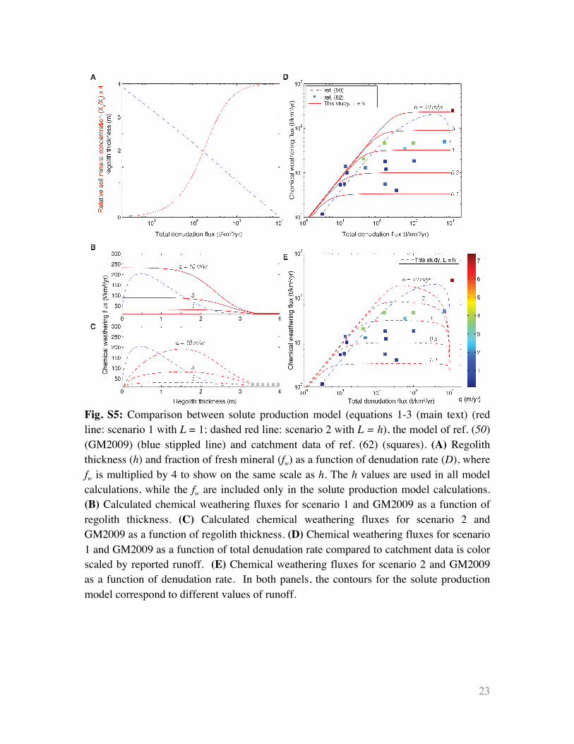
Fig. S5: Comparison between solute production model (equations 1-3 (main text) (red line: scenario 1 with L = 1; dashed red line: scenario 2 with L = h), the model of ref. (50) (GM2009) (blue stippled line) and catchment data of ref. (62) (squares). (A) Regolith thickness (h) and fraction of fresh mineral (fw) as a function of denudation rate (D), where fw is multiplied by 4 to show on the same scale as h. The h values are used in all model calculations, while the fw are included only in the solute production model calculations. (B) Calculated chemical weathering fluxes for scenario 1 and GM2009 as a function of regolith thickness. (C) Calculated chemical weathering fluxes for scenario 2 and GM2009 as a function of regolith thickness. (D) Chemical weathering fluxes for scenario 1 and GM2009 as a function of total denudation rate compared to catchment data is color scaled by reported runoff. (E) Chemical weathering fluxes for scenario 2 and GM2009 as a function of denudation rate. In both panels, the contours for the solute production model correspond to different values of runoff.

24

Fig. S6: (A) SiO2(aq) flux as a function of total denudation flux for the data of ref. (8) and the steady state RTM simulations (green shaded region), which represent the maximum flux. The data is compared to scenario 1 from Fig. S5, which imposes a relationship between h, erosion rate and L. This demonstrates reasonable correspondence between maximum calculated SiO2 and rates used in RTM of Fig. S2 and measured fluxes and illustrates the agreement between the runoff contours of the model and the actual data. (B) Dw as a function of SiO2(aq) flux for rivers compared to scenarios 1 and 2 from Fig. S5 with contours corresponding to different runoff values. (C) Dw values calculated for each river are compared to erosional fluxes based on total suspended solid flux (ref. (8)) and both total suspended and cosmogenic nuclides for rivers of ref. (62), where Dw is calculated independent of erosion rate using equation (3) (main text). The rivers are color scaled by the SiO2(aq) flux. For the river data, the weak correlation between erosion rate and Dw, assuming a power law relationship (not shown), is Dw [yr] = 0.0018E[t/km2/yr]0.56 (R² = 0.40, P<0.0001).

25

Kaolinite + 6H+ —> 2Al3+ + 2SiO2(aq) + 5H2OAnorthite +2CO2 +3H2O —> Ca2+ + Kaolinite +2HCO3-

Albite + 4H+ —> Na+ + Al3+ + 3SiO2(aq) + 2H2O

K-spar + 4H+ —> K+ + Al3+ + 3SiO2(aq) + 2H2O

CO2(g) + H2O --> H+ + HCO3-

2Albite + 2CO2(g)+ 3H2O —> Kaolinite + 4SiO2(aq) + 2Na+ + 2HCO3-

2Albite + 2CO2(g) + 3H2O--> Halloysite + 4SiO2(aq) + 2Na+ + 2HCO3-

Plag(An20) + 4.8H +—> 1.2Al3+ + 0.8Na ++ 0.2Ca2+ + 2.8SiO2(aq) + 2.4H2O

1.67Plag(An20) + 2CO2(g) + 3H2O—>Halloysite + 2.47Na ++ 0.33Ca2+ + 2.8SiO2(aq) + 2HCO3-

Log

K

-25

-20

-15

-10

-5

0

5

10

10 20 30 40 50Temperature (˚C)

Fig. S7: Temperature sensitivity of weathering reactions. The primary mineral dissolution reactions and CO2 dissociation reactions are show in solid lines, while the net reactions are shown in light stippled lines. The starred reaction in bold represents a simplified version of the one of the net reaction considered in the RTM simulation. Thermodynamic data is from ref. (92).

26

Fig. S8: Sensitivity analysis of solute production model to changes in Ceq and Teq due to lithology or temperature, respectively. (A) A 50% increase in the global maximum equilibrium concentration, Ceq (blue stippled lines) shown relative to the original model (black lines). (B) Increases in keff by a factor of 2, 5 and 10 (see legend) corresponding to temperature increases of 15 to 30˚C and 15 to 40˚C and 15 to 75˚C, respectively. Because keff appears in both the Rn term and the fw term (i.e., in the numerator and the denominator of Dw) the effects of temperature are minimal at small Dw, but increase with increasing Dw as the numerator becomes larger. (C) and (D) Sensitivity analysis is shown in comparison to basalt data from ref. (84) where model calculations are converted to chemical weathering rate as in Fig. S5.

27

Table S1: Definition of model parameters along with units and formulae. The parameter values assumed in calculations are provided in italics within parentheses, while variables are indicated as such. Lower case values provided in the text for ceq, c0, l and tf correspond to the 1-D case are not used outside of the derivation. Parameter Definition Units Formula (Value) W Chemical denudation t/km2/yr Variable E Physical denudation t/km2/yr Variable D Total denudation t/km2/yr D = E + W P Soil production t/km2/yr Variable Ceq Thermodynamic limit

(global maximum) µmol/L Theoretical (RTM model):

(380 µmol/L SiO2) 95% Conf. (Table 1): (375 µmol/L SiO2)a (327 µmol/L SiO2) b

C0 Initial concentration µmol /L (0 µmol /L) L Flow path length meters Variable Ls Soil/weathering

thickness meters Variable

φ Porosity [-] Variable (0.175 in RTM) q Flow rate m/yr Variable τ Scaling parameter (en) [-] en, n = 2 ρsf Mass mineral/fluid

volume ratio g/L = 1000*ρb/φ (12728 g/L in RTM)

where ρb = 2.23 g/cm3 M Mass of soil profile g Variable m Molar mass g/mol (270 g/mol) keff Net rate constant mol/m2/yr (8.7 x 10-6 mol/m2/yr) A Specific surface area m2/g (0.1 m2/ g in RTM) Xr Mineral concentration

in fresh rock (reactive only)

gmin/gsoil (0.36 in RTM) (17.8 wt% K-spar and 18.2 wt % Plag (An20))

Xs Mineral concentration in soil (reactive only)

gmin/gsoil =Xr/(1+(mkeffATs))

fw Mass depletion fraction [-] = Xs/Xr =1/ (1+mkeffATs) Rn, max Maximum net reaction

rate µmol /L/yr Theoretical (RTM model):

= ρsf keffAXr (1085 µmol/L/yr SiO2)

Rn, Net reaction rate µmol /L/yr = Rn, max * fw Ts Soil residence time yr Soil age, or: Ls/P Tf Mean fluid residence

time yr ≈ L φ /q

Teq Equilibrium Time yr ≈ Ceq/(Rn,max*fw) a For rivers from ref. (8), value used in main text for Figs. 1, 2, 3.

b For rivers from from ref. (60).

References and Notes 1. C. Sagan, G. Mullen, Earth and Mars: Evolution of atmospheres and surface temperatures.

Science 177, 52–56 (1972). doi:10.1126/science.177.4043.52 Medline

2. J. C. G. Walker, P. B. Hays, J. F. Kasting, A negative feedback mechanism for the long-term stabilization of Earth’s surface temperature. J. Geophys. Res. 86, (C10), 9776 (1981). doi:10.1029/JC086iC10p09776

3. R. A. Berner, Z. Kothavala, GEOCARB III: A revised model of atmospheric CO2 over Phanerozoic time. Am. J. Sci. 301, 182–204 (2001). doi:10.2475/ajs.301.2.182

4. R. A. Berner, A. C. Lasaga, R. M. Garrels, The carbonate-silicate geochemical cycle and its effect on atmospheric carbon dioxide over the past 100 million years. Am. J. Sci. 283, 641–683 (1983). doi:10.2475/ajs.283.7.641

5. L. R. Kump, S. L. Brantley, M. A. Arthur, Chemical weathering, atmospheric CO2, and climate. Annu. Rev. Earth Planet. Sci. 28, 611–667 (2000). doi:10.1146/annurev.earth.28.1.611

6. R. A. Berner, K. Caldeira, The need for mass balance and feedback in the geochemical carbon cycle. Geology 25, 955 (1997). doi:10.1130/0091-7613(1997)025<0955:TNFMBA>2.3.CO;2

7. L. R. Kump, M. A. Arthur, in Tectonics Uplift and Climate Change, W. F. Ruddiman, Ed. (Plenum Publishing Co., 1997), pp. 399–426.

8. J. Gaillardet, B. Dupre, P. Louvat, C. J. Allegre, Global silicate weathering and CO2 consumption rates deduced from the chemistry of large rivers. Chem. Geol. 159, 3–30 (1999). doi:10.1016/S0009-2541(99)00031-5

9. J. K. Willenbring, F. von Blanckenburg, Long-term stability of global erosion rates and weathering during late-Cenozoic cooling. Nature 465, 211–214 (2010). doi:10.1038/nature09044 Medline

10. J. M. Edmond, Y. S. Huh, in Tectonics Uplift and Climate Change, W. F. Ruddiman, Ed. (Plenum Publishing Co., 1997), p. 558.

11. M. Pagani, K. Caldeira, R. Berner, D. J. Beerling, The role of terrestrial plants in limiting atmospheric CO2 decline over the past 24 million years. Nature 460, 85–88 (2009). doi:10.1038/nature08133 Medline

12. S. E. McCauley, D. J. DePaolo, in Global Tectonics and Climate Change, W. F. Ruddiman, W. Prell, Eds. (Plenum Press, 1997), pp. 428–465.

13. Methods and a complete description of the model are available on Science Online.

14. G. Li, H. Elderfield, Evolution of carbon cycle over the past 100 million years. Geochim. Cosmochim. Acta 103, 11–25 (2013). doi:10.1016/j.gca.2012.10.014

15. D. F. Boucher, G. E. Alves, Chem. Eng. Prog. 55, 55 (1959).

16. K. Maher, The role of fluid residence time and topographic scales in determining chemical fluxes from landscapes. Earth Planet. Sci. Lett. 312, 48–58 (2011). doi:10.1016/j.epsl.2011.09.040

17. K. Yoo, S. M. Mudd, Discrepancy between mineral residence time and soil age: Implications for the interpretation of chemical weathering rates. Geology 36, 35 (2008). doi:10.1130/G24285A.1

18. G. E. Hilley, C. P. Chamberlain, S. Moon, S. Porder, S. D. Willett, Competition between erosion and reaction kinetics in controlling silicate-weathering rates. Earth Planet. Sci. Lett. 293, 191–199 (2010). doi:10.1016/j.epsl.2010.01.008

19. K. L. Ferrier, J. W. Kirchner, Effects of physical erosion on chemical denudation rates: A numerical modeling study of soil-mantled hillslopes. Earth Planet. Sci. Lett. 272, 591–599 (2008). doi:10.1016/j.epsl.2008.05.024

20. S. Brantley, M. I. Lebedeva, Learning to read the chemistry of regolith to understand the critical zone. Annu. Rev. Earth Planet. Sci. 39, 387–416 (2011). doi:10.1146/annurev-earth-040809-152321

21. Independent calculation of Dw coefficients via Eq. 1 would be one approach. At present, sufficient data for large rivers is not available.

22. To compute the curves in Figs. 1 to 3, we use the concentration and discharge data of ref. (8), Rn,max of 1085 μmol SiO2/L/yr and a maximum Ceq of 375 μmol/L (table S1) to determine the fluxes and Dw contours associated with the global rivers, mostly draining granitic lithologies. Basaltic lithologies are expected to follow the same general behavior (fig. S8). In Fig. 1 we show contours of Ts corresponding to Dw contours in Figs. 2 and 3. The contours of Dw, which do not depend on the absolute values of Rn, fw or Ts, illustrate how rivers respond in a relative sense to climatic and tectonic variations.

23. G. J. S. Bluth, L. R. Kump, Lithologic and climatologic controls of river chemistry. Geochim. Cosmochim. Acta 58, 2341–2359 (1994). doi:10.1016/0016-7037(94)90015-9

24. S. E. Godsey, J. W. Kirchner, D. W. Clow, Concentration-discharge relationships reflect chemostatic characteristics of US catchments. Hydrol. Processes 23, 1844–1864 (2009). doi:10.1002/hyp.7315

25. R. F. Stallard, J. M. Edmond, Geochemistry of the Amazon: 2. The influence of geology and weathering environment on the dissolved load. J. Geophys. Res. 88, (C14), 9671 (1983). doi:10.1029/JC088iC14p09671

26. M. E. Raymo, W. F. Ruddiman, Tectonic forcing of late Cenozoic climate. Nature 359, 117–122 (1992). doi:10.1038/359117a0

27. A. J. West, Thickness of the chemical weathering zone and implications for erosional and climatic drivers of weathering and for carbon-cycle feedbacks. Geology 40, 811–814 (2012). doi:10.1130/G33041.1

28. S. D. Willett, Orogeny and orography: The effects of erosion on the structure of mountain belts. J. Geophys. Res. 104, (B12), 28957 (1999). doi:10.1029/1999JB900248

29. A. J. West, M. J. Bickle, R. Collins, J. Brasington, Small-catchment perspective on Himalayan weathering fluxes. Geology 30, 355 (2002). doi:10.1130/0091-7613(2002)030<0355:SCPOHW>2.0.CO;2

30. J. Bouchez, J. Gaillardet, M. Lupker, P. Louvat, C. France-Lanord, L. Maurice, E. Armijos, J.-S. Moquet, Floodplains of large rivers: Weathering reactors or simple silos? Chem. Geol. 332-333, 166–184 (2012). doi:10.1016/j.chemgeo.2012.09.032

31. S. Manabe, R. T. Wetherald, P. C. D. Milly, T. L. Delworth, R. J. Stouffer, Century-scale change in water availability: CO2-quadrupling experiment. Clim. Change 64, 59–76 (2004). doi:10.1023/B:CLIM.0000024674.37725.ca

32. D. R. Montgomery, M. T. Brandon, Topographic controls on erosion rates in tectonically active mountain ranges. Earth Planet. Sci. Lett. 201, 481–489 (2002). doi:10.1016/S0012-821X(02)00725-2

33. R. A. Berner, Rate control of mineral dissolution under earth surface conditions. Am. J. Sci. 278, 1235–1252 (1978). doi:10.2475/ajs.278.9.1235

34. K. Maher, The dependence of chemical weathering rates on fluid residence time. Earth Planet. Sci. Lett. 294, 101–110 (2010). doi:10.1016/j.epsl.2010.03.010

35. J. J. McDonnell, K. McGuire, P. Aggarwal, K. J. Beven, D. Biondi, G. Destouni, S. Dunn, A. James, J. Kirchner, P. Kraft, S. Lyon, P. Maloszewski, B. Newman, L. Pfister, A. Rinaldo, A. Rodhe, T. Sayama, J. Seibert, K. Solomon, C. Soulsby, M. Stewart, D. Tetzlaff, C. Tobin, P. Troch, M. Weiler, A. Western, A. Worman, S. Wrede, How old is streamwater? Open questions in catchment transit time conceptualization, modelling and analysis. Hydrol. Processes 24, 1745–1754 (2010). doi:10.1002/hyp.7796

36. P. Małoszewski, A. Zuber, Determining the turnover time of groundwater systems with the aid of environmental tracers. 1. Models and their applicability. J. Hydrol. (Amst.) 57, 207–231 (1982). doi:10.1016/0022-1694(82)90147-0

37. P. Aagaard, H. C. Helgeson, Thermodynamic and kinetic constraints on reaction-rates among minerals and aqueous-solutions. 1. Theoretical considerations. Am. J. Sci. 282, 237–285 (1982). doi:10.2475/ajs.282.3.237

38. C. I. Steefel, K. Maher, in Reviews in Mineralogy & Geochemistry (Mineralogical Society of America), vol. 70, pp. 485–532 (2009).

39. J. W. Kirchner, D. Tetzlaff, C. Soulsby, Comparing chloride and water isotopes as hydrological tracers in two Scottish catchments. Hydrol. Processes 24, 1631–1645 (2010). doi:10.1002/hyp.7676

40. K. J. McGuire, J. J. McDonnell, A review and evaluation of catchment transit time modeling. J. Hydrol. (Amst.) 330, 543–563 (2006). doi:10.1016/j.jhydrol.2006.04.020

41. G. Botter, E. Bertuzzo, A. Rinaldo, Transport in the hydrologic response: Travel time distributions, soil moisture dynamics, and the old water paradox. Water Resour. Res. 46, W03514 (2010). doi:10.1029/2009WR008371

42. G. Botter, E. Bertuzzo, A. Rinaldo, Catchment residence and travel time distributions: The master equation. Geophys. Res. Lett. 38, L11403 (2011). doi:10.1029/2011GL047666

43. A. Rinaldo, A. Marani, Basin scale model of solute transport. Water Resour. Res. 23, 2107–2118 (1987). doi:10.1029/WR023i011p02107

44. A. Rinaldo, K. J. Beven, E. Bertuzzo, L. Nicotina, J. Davies, A. Fiori, D. Russo, G. Botter, Catchment travel time distributions and water flow in soils. Water Resour. Res. 47, W07537 (2011). doi:10.1029/2011WR010478

45. D. J. Goode, Direct simulation of groundwater age. Water Resour. Res. 32, 289–296 (1996). doi:10.1029/95WR03401

46. N. B. Engdahl, T. R. Ginn, G. E. Fogg, Non-Fickian dispersion of groundwater age. Water Resour. Res. 48, W07508 (2012). doi:10.1029/2012WR012251

47. G. Blöschl, M. Sivapalan, Sale issues in hydrological modeling - A review. Hydrol. Processes 9, 251–290 (1995). doi:10.1002/hyp.3360090305

48. W. A. Jury, Simulation of solute transport using a transfer-function model. Water Resour. Res. 18, 363–368 (1982). doi:10.1029/WR018i002p00363

49. J. R. Waldbauer, C. P. Chamberlain, in Ecological Studies 177: A History of Atmospheric CO2 and Its Effects on Plants, Animals and Ecosystems (Springer Verlag, 2005), pp. 166–184.

50. E. J. Gabet, S. M. Mudd, A theoretical model coupling chemical weathering rates with denudation rates. Geology 37, 151–154 (2009). doi:10.1130/G25270A.1

51. M. E. Raymo, The Himalayas, organic-carbon burial, and climate in the Miocene. Paleoceanography 9, 399–404 (1994). doi:10.1029/94PA00289

52. M. I. Lebedeva, R. C. Fletcher, S. L. Brantley, A mathematical model for steadystate regolith production at constant erosion rate. Earth Surf. Processes 35, 508–524 (2010).

53. J. Moore, P. C. Lichtner, A. F. White, S. L. Brantley, Using a reactive transport model to elucidate differences between laboratory and field dissolution rates in regolith. Geochim. Cosmochim. Acta 93, 235–261 (2012). doi:10.1016/j.gca.2012.03.021

54. K. Maher, C. I. Steefel, A. F. White, D. A. Stonestrom, The role of reaction affinity and secondary minerals in regulating chemical weathering rates at the Santa Cruz Soil Chronosequence, California. Geochim. Cosmochim. Acta 73, 2804–2831 (2009). doi:10.1016/j.gca.2009.01.030

55. C. S. Riebe, J. W. Kirchner, R. C. Finkel, Long-term rates of chemical weathering and physical erosion from cosmogenic nuclides and geochemical mass balance. Geochim. Cosmochim. Acta 67, 4411–4427 (2003). doi:10.1016/S0016-7037(03)00382-X

56. A. F. White, S. L. Brantley, The effect of time on the weathering of silicate minerals: Why do weathering rates differ in the laboratory and field? Chem. Geol. 202, 479–506 (2003). doi:10.1016/j.chemgeo.2003.03.001

57. K. Maher, D. J. DePaolo, J. C. F. Lin, Rates of silicate dissolution in deep-sea sediment: In situ measurement using U234/U238 of pore fluids. Geochim. Cosmochim. Acta 68, 4629–4648 (2004). doi:10.1016/j.gca.2004.04.024

58. W. E. Glassley, A. M. Simmons, J. R. Kercher, Mineralogial heterogeneity in fractured, porous media and its representation in reactive transport models. Appl. Geochem. 17, 699–708 (2002). doi:10.1016/S0883-2927(02)00031-8

59. L. Li, C. I. Steefel, M. B. Kowalsky, A. Englert, S. S. Hubbard, Effects of physical and geochemical heterogeneities on mineral transformation and biomass accumulation during biostimulation experiments at Rifle, Colorado. J. Contam. Hydrol. 112, 45–63 (2010). doi:10.1016/j.jconhyd.2009.10.006 Medline

60. J. L. Dixon, F. von Blanckenburg, Soils as pacemakers and limiters of global silicate weathering. C. R. Geosci. 344, 597–609 (2012). doi:10.1016/j.crte.2012.10.012

61. A. F. White, A. E. Blum, Effects of climate on chemical weathering in watersheds. Geochim. Cosmochim. Acta 59, 1729–1747 (1995). doi:10.1016/0016-7037(95)00078-E

62. A. J. West, A. Galy, M. Bickle, Tectonic and climatic controls on silicate weathering. Earth Planet. Sci. Lett. 235, 211–228 (2005). doi:10.1016/j.epsl.2005.03.020

63. H. C. Helgeson, in The Feldspars, W. S. MacKenzie, J. Zussman, Eds. (Manchester Univ. Press, 1974), pp. 184–217.

64. J. L. Dixon, A. S. Hartshorn, A. M. Heimsath, R. A. DiBiase, K. X. Whipple, Chemical weathering response to tectonic forcing: A soils perspective from the San Gabriel Mountains, California. Earth Planet. Sci. Lett. 323-324, 40–49 (2012). doi:10.1016/j.epsl.2012.01.010

65. H. C. Helgeson, W. M. Murphy, P. Aagaard, Thermodynamic and kinetic constraints on reaction rates among minerals and aqueous-solutions. 2. Rate constants, effective surface area, and the hydrolysis of feldspar. Geochim. Cosmochim. Acta 48, 2405–2432 (1984). doi:10.1016/0016-7037(84)90294-1

66. R. M. Garrels, F. T. Mackenzie, Origin of the chemical compositions of some springs and lakes. Adv. Chem. Ser. 67, 222–242 (1967). doi:10.1021/ba-1967-0067.ch010

67. A. C. Lasaga, R. A. Berner, Fundamental aspects of quantitative models for geochemical cycles. Chem. Geol. 145, 161–175 (1998). doi:10.1016/S0009-2541(97)00142-3

68. A. F. White, M. S. Schulz, D. A. Stonestrom, D. V. Vivit, J. Fitzpatrick, T. D. Bullen, K. Maher, A. E. Blum, Chemical weathering of a marine terrace chronosequence, Santa Cruz, California. Part II: Solute profiles, gradients and the comparisons of contemporary and long-term weathering rates. Geochim. Cosmochim. Acta 73, 2769–2803 (2009). doi:10.1016/j.gca.2009.01.029

69. S. L. Brantley, J. Bandstra, J. Moore, A. F. White, Modelling chemical depletion profiles in regolith. Geoderma 145, 494–504 (2008). doi:10.1016/j.geoderma.2008.02.010

70. P. C. Lichtner, Scaling properites of time-space kinetic mass transport equations and the local equilibrium limit. Am. J. Sci. 293, 257–296 (1993). doi:10.2475/ajs.293.4.257

71. G. J. Kenoyer, C. J. Bowser, Groundwater chemical evolution in a sandy silicate aquifer in northern Wisconsin. 1. Patterns and rates of change. Water Resour. Res. 28, 579–589 (1992). doi:10.1029/91WR02302

72. G. J. Kenoyer, C. J. Bowser, Groundwater chemical evolution in a sandy silicate aquifer in northern Wisconsin. 2. Reaction modeling. Water Resour. Res. 28, 591–600 (1992). doi:10.1029/91WR02303

73. D. W. Clow, M. A. Mast, Mechanisms for chemostatic behavior in catchments: Implications for CO2 consumption by mineral weathering. Chem. Geol. 269, 40–51 (2010). doi:10.1016/j.chemgeo.2009.09.014

74. J. Gaillardet, S. Rad, K. Rive, P. Louvat, C. Gorge, C. J. Allegre, E. Lajeunesse, Orography-driven chemical denudation in the Lesser Antilles: Evidence for a new feed-back mechanism stabilizing atmospheric CO2. Am. J. Sci. 311, 851–894 (2011). doi:10.2475/10.2011.02

75. J. B. Shanley, W. H. McDowell, R. F. Stallard, Long-term patterns and short-term dynamics of stream solutes and suspended sediment in a rapidly weathering tropical watershed. Water Resour. Res. 47, W07515 (2011). doi:10.1029/2010WR009788

76. J. Hartmann, N. Jansen, H. H. Durr, A. Harashima, K. Okubo, S. Kempe, Predicting riverine dissolved silica fluxes to coastal zones from a hyperactive region and analysis of their first-order controls. Int. J. Earth Sci. 99, 207–230 (2010). doi:10.1007/s00531-008-0381-5

77. E. S. Eiriksdottir, S. R. Gislason, E. H. Oelkers, Does temperature or runoff control the feedback between chemical denudation and climate? Insights from NE Iceland. Geochim. Cosmochim. Acta 107, 65–81 (2013). doi:10.1016/j.gca.2012.12.034

78. M. A. Velbel, Temperature-dependence of silicate weathering in nature - how strong a negative feedback on long-term accumulation of atmospheric CO2 and global greenhouse warming. Geology 21, 1059–1062 (1993). doi:10.1130/0091-7613(1993)021<1059:TDOSWI>2.3.CO;2

79. H. C. Helgeson, J. M. Delany, H. W. Nesbitt, D. K. Bird, Summary and critique of the thermodynamic properties of rock-forming minerals. Am. J. Sci. 278, 1–229 (1978).

80. D. D. Eberl, V. C. Farmer, R. M. Barrer, Clay mineral formation and transformation in rocks and soils. Philos. Trans. R. Soc. London Ser. A 311, 241–257 (1984). doi:10.1098/rsta.1984.0026

81. A. C. Lasaga, Rev. Mineral. Geochem. 31, 23–86 (1995).

82. A. F. White, A. E. Blum, T. D. Bullen, D. V. Vivit, M. Schulz, J. Fitzpatrick, The effect of temperature on experimental and natural chemical weathering rates of granitoid rocks. Geochim. Cosmochim. Acta 63, 3277–3291 (1999). doi:10.1016/S0016-7037(99)00250-1

83. J. L. Palandri, Y. K. Kharaka, A compilation of rate parameters of water-mineral interaction kinetics for application to geochemical modeling. U.S. Geol. Surv. Open-File Rep. 2004-1068 (2004).

84. C. Dessert, B. Dupre, J. Gaillardet, L. M. Francois, C. J. Allegre, Basalt weathering laws and the impact of basalt weathering on the global carbon cycle. Chem. Geol. 202, 257–273 (2003). doi:10.1016/j.chemgeo.2002.10.001

85. J. Dessert, J. Gaillardet, B. Dupre, J. Schott, O. S. Pokrovsky, Fluxes of high- versus low-temperature water-rock interactions in aerial volcanic areas: Example from the Kamchatka Peninsula, Russia. Geochim. Cosmochim. Acta 73, 148–169 (2009). doi:10.1016/j.gca.2008.09.012

86. S. Moon, C. P. Chamberlain, K. Blisniuk, N. Levine, D. H. Rood, G. E. Hilley, Climatic control of denudation in the deglaciated landscape of the Washington Cascades. Nat. Geosci. 4, 469–473 (2011). doi:10.1038/ngeo1159

87. J. Hartmann, N. Jansen, H. H. Durr, S. Kempe, P. Kohler, Global CO2-consumption by chemical weathering: What is the contribution of highly active weathering regions? Global Planet. Change 69, 185–194 (2009). doi:10.1016/j.gloplacha.2009.07.007

88. B. Dupré, C. Dessert, P. Oliva, Y. Godderis, J. Viers, L. Francois, R. Millot, J. Gaillardet, Rivers, chemical weathering, and Earth's climate. C. R. Geosci. 335, 1141–1160 (2003). doi:10.1016/j.crte.2003.09.015

89. J. Hartmann, Bicarbonate-fluxes and CO2-consumption by chemical weathering on the Japanese Archipelago - Application of a multi-lithological model framework. Chem. Geol. 265, 237–271 (2009). doi:10.1016/j.chemgeo.2009.03.024

90. S. Solomon, D. Qin, M. Manning, Z. Chen, M. Marquis, K. B. Averyt, M. Tignor, H. L. Miller, Eds., Climate Change 2007 - The Physical Science Basis. Contribution of Working Group I to the Fourth Assessment Report of the Intergovernmental Panel on Climate Change (Cambridge Univ. Press, Cambridge, UK and New York, 2007).

91. M. Pagani, Z. Liu, J. LaRiviere, A. C. Ravelo, High Earth-system climate sensitivity determined from Pliocene carbon dioxide concentrations. Nat. Geosci. 3, 27–30 (2010). doi:10.1038/ngeo724

92. J. W. Johnson, E. H. Oelkers, H. C. Helgeson, SUPCRT92: A software package for calculating the standard molal thermodynamic properties of minerals, gases, aqueous species, and reactions from 1 to 5000 bar and 0 to 1000°C. Comput. Geosci. 18, 899–947 (1992). doi:10.1016/0098-3004(92)90029-Q