SUPPLEMENTARY Work Measurement, Learning … Outline Work Measurement OM Spotlight: Work Measurement Activities in Roller Coaster Maintenance Time Study Methods OM Spotlight: Job Description—

Chapter Outline

Work Measurement

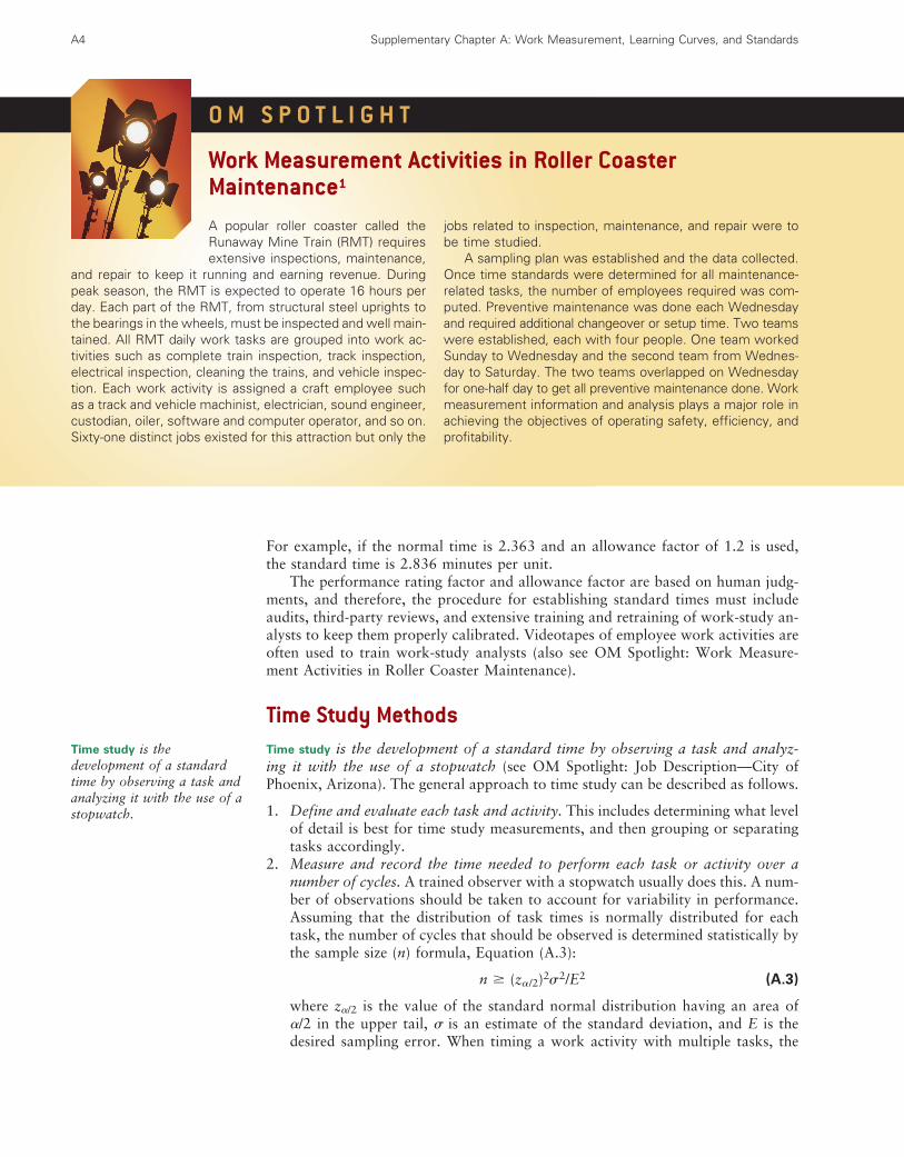
OM Spotlight: WorkMeasurement Activities inRoller Coaster Maintenance

Time Study MethodsOM Spotlight: Job Description—

City of Phoenix, Arizona

Operations Analyst for City ofPhoenix, Arizona

Predetermined Time StandardMethods

Learning Curves

Practical Issues in Using LearningCurves

Solved ProblemsKey Terms and ConceptsQuestions for Review and

DiscussionProblems and ActivitiesCases

Rehabilitation Hospital ofFlorida

The State versus John BracketEndnotes

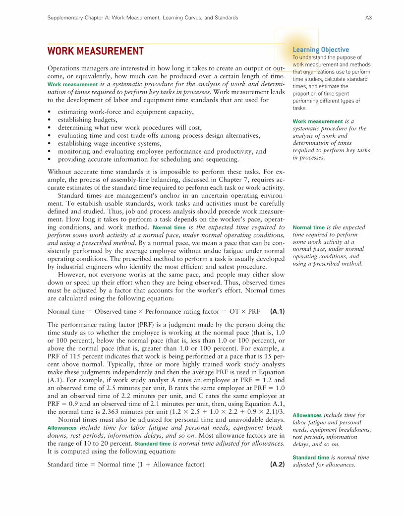
Learning Objectives

• To understand the purpose of work measurement and methodsthat organizations use to perform time studies, calculate standardtimes, and estimate the proportion of time spent performing differ-ent types of tasks.

• To understand the concept of learning curves and how they can affect business decisions, and to learn computational methods forestimating aggregate production times in learning environments.

Work Measurement,Learning Curves, andStandards

SUPPLEMENTARYCHAPTER A

• “John Bracket has filed a lawsuit against us, George,” stated Paul Cumin, thevice president of operations for the State Rehabilitation Services Commission(SRSC). “George, you are Bracket’s manager. So what happened? He claimsyou raised his daily productivity quota for processing invoices from 200 to 300.”“Paul, I did raise his quota to more closely match the other employees. Bracketis always late for work, plays games on the computer, violates our dress code,and is generally disliked by his peer employees,” responded George Davis,Bracket’s immediate supervisor. “Is there any logic or numerical basis for yourincreasing his quota?” Paul asked him. As he left the room, George responded,“Paul, I’ll get my work study data out, review it, and get back to you this afternoon.”

• “Jim, it takes 2,000 hours to build each electrical generating turbine, so if wehave to build ten, it takes 20,000 hours. We should plan our budget and price pergenerator based on 20,000 hours,” exclaimed Pete Jacobs, the vice presidentof finance. “No, Pete. According to my calculations, it will take only 14,232hours to build ten turbines and our total cost and budget will be much lowerthan you think,” said Jim Conner, the vice president of operations. “How doyou get such crazy numbers?” replied Jacobs.

Time standards represent reasonable estimates of the amount of time needed to per-form a task based on an analysis of the work by a trained industrial engineer orother operations expert. The first episode highlights the importance of time stan-dards in setting job performance standards, and how they can affect management-labor relations. Bracket’s new processing quota of 300 invoices per day may or maynot be a fair job performance goal, but the only way to find out is through care-ful work measurement analysis. You will have the opportunity to analyze this sit-uation in more detail in one of the cases at the end of this chapter.

In the second episode, Jacobs cannot understand the discrepancy between hisestimate of 20,000 hours and Conner’s value of 14,232 hours to produce a batchof turbines. The assembly of electrical power-generating turbines is a complex jobwith labor costs for engineers and production employees approaching $100 perhour. Obviously, a difference of 5,768 hours can be significant in terms of cost,budgets, and pricing decisions. Where did Conner get his figure? Moreover, whyshould the total time to produce ten turbines be less than 10 times the time to pro-duce the first? Many work tasks show increased performance over time because oflearning and improvement. Failure to recognize this can lead to poor budgeting,erroneous promises for delivery, and other bad management decisions.

In this supplemental chapter we introduce work measurement, standards, andlearning curves, and how they are used in business. Most large corporations de-velop standard times for routine work tasks using work measurement. They areused in setting job performance standards, establishing recognition and reward pro-grams, and for compensation incentives. Valid standard times are vital to accom-plishing most of the process design and operations analysis methods described inthis text. Smaller businesses, especially service businesses, usually do not have suchstandard times for their work activities and tasks. However, if one seeks to improveoperations, analyzing work and determining standard times for key work activitiesand processes is a crucial first step.

A2

Supplementary Chapter A: Work Measurement, Learning Curves, and Standards A3

Learning ObjectiveTo understand the purpose ofwork measurement and methodsthat organizations use to performtime studies, calculate standardtimes, and estimate theproportion of time spentperforming different types oftasks.

Work measurement is asystematic procedure for theanalysis of work anddetermination of timesrequired to perform key tasksin processes.

WORK MEASUREMENTOperations managers are interested in how long it takes to create an output or out-come, or equivalently, how much can be produced over a certain length of time.Work measurement is a systematic procedure for the analysis of work and determi-nation of times required to perform key tasks in processes. Work measurement leadsto the development of labor and equipment time standards that are used for

• estimating work-force and equipment capacity,• establishing budgets,• determining what new work procedures will cost,• evaluating time and cost trade-offs among process design alternatives,• establishing wage-incentive systems,• monitoring and evaluating employee performance and productivity, and• providing accurate information for scheduling and sequencing.

Without accurate time standards it is impossible to perform these tasks. For ex-ample, the process of assembly-line balancing, discussed in Chapter 7, requires ac-curate estimates of the standard time required to perform each task or work activity.

Standard times are management’s anchor in an uncertain operating environ-ment. To establish usable standards, work tasks and activities must be carefullydefined and studied. Thus, job and process analysis should precede work measure-ment. How long it takes to perform a task depends on the worker’s pace, operat-ing conditions, and work method. Normal time is the expected time required toperform some work activity at a normal pace, under normal operating conditions,and using a prescribed method. By a normal pace, we mean a pace that can be con-sistently performed by the average employee without undue fatigue under normaloperating conditions. The prescribed method to perform a task is usually developedby industrial engineers who identify the most efficient and safest procedure.

However, not everyone works at the same pace, and people may either slowdown or speed up their effort when they are being observed. Thus, observed timesmust be adjusted by a factor that accounts for the worker’s effort. Normal timesare calculated using the following equation:

Normal time � Observed time � Performance rating factor � OT � PRF (A.1)

The performance rating factor (PRF) is a judgment made by the person doing thetime study as to whether the employee is working at the normal pace (that is, 1.0or 100 percent), below the normal pace (that is, less than 1.0 or 100 percent), orabove the normal pace (that is, greater than 1.0 or 100 percent). For example, aPRF of 115 percent indicates that work is being performed at a pace that is 15 per-cent above normal. Typically, three or more highly trained work study analystsmake these judgments independently and then the average PRF is used in Equation(A.1). For example, if work study analyst A rates an employee at PRF � 1.2 andan observed time of 2.5 minutes per unit, B rates the same employee at PRF � 1.0and an observed time of 2.2 minutes per unit, and C rates the same employee atPRF � 0.9 and an observed time of 2.1 minutes per unit, then, using Equation A.1,the normal time is 2.363 minutes per unit (1.2 � 2.5 � 1.0 � 2.2 � 0.9 � 2.1)/3.

Normal times must also be adjusted for personal time and unavoidable delays.Allowances include time for labor fatigue and personal needs, equipment break-downs, rest periods, information delays, and so on. Most allowance factors are inthe range of 10 to 20 percent. Standard time is normal time adjusted for allowances.It is computed using the following equation:

Standard time � Normal time (1 � Allowance factor) (A.2)

Normal time is the expectedtime required to performsome work activity at anormal pace, under normaloperating conditions, andusing a prescribed method.

Allowances include time forlabor fatigue and personalneeds, equipment breakdowns,rest periods, informationdelays, and so on.

Standard time is normal timeadjusted for allowances.

For example, if the normal time is 2.363 and an allowance factor of 1.2 is used,the standard time is 2.836 minutes per unit.

The performance rating factor and allowance factor are based on human judg-ments, and therefore, the procedure for establishing standard times must includeaudits, third-party reviews, and extensive training and retraining of work-study an-alysts to keep them properly calibrated. Videotapes of employee work activities areoften used to train work-study analysts (also see OM Spotlight: Work Measure-ment Activities in Roller Coaster Maintenance).

Time Study MethodsTime study is the development of a standard time by observing a task and analyz-ing it with the use of a stopwatch (see OM Spotlight: Job Description—City ofPhoenix, Arizona). The general approach to time study can be described as follows.

1. Define and evaluate each task and activity. This includes determining what levelof detail is best for time study measurements, and then grouping or separatingtasks accordingly.

2. Measure and record the time needed to perform each task or activity over anumber of cycles. A trained observer with a stopwatch usually does this. A num-ber of observations should be taken to account for variability in performance.Assuming that the distribution of task times is normally distributed for eachtask, the number of cycles that should be observed is determined statistically bythe sample size (n) formula, Equation (A.3):

n � (z�/2)2�2/E2 (A.3)

where z�/2 is the value of the standard normal distribution having an area of�/2 in the upper tail, � is an estimate of the standard deviation, and E is thedesired sampling error. When timing a work activity with multiple tasks, the

A4 Supplementary Chapter A: Work Measurement, Learning Curves, and Standards

O M S P O T L I G H T

Work Measurement Activities in Roller Coaster Maintenance1

A popular roller coaster called theRunaway Mine Train (RMT) requiresextensive inspections, maintenance,

and repair to keep it running and earning revenue. Duringpeak season, the RMT is expected to operate 16 hours perday. Each part of the RMT, from structural steel uprights tothe bearings in the wheels, must be inspected and well main-tained. All RMT daily work tasks are grouped into work ac-tivities such as complete train inspection, track inspection,electrical inspection, cleaning the trains, and vehicle inspec-tion. Each work activity is assigned a craft employee suchas a track and vehicle machinist, electrician, sound engineer,custodian, oiler, software and computer operator, and so on.Sixty-one distinct jobs existed for this attraction but only the

jobs related to inspection, maintenance, and repair were tobe time studied.

A sampling plan was established and the data collected.Once time standards were determined for all maintenance-related tasks, the number of employees required was com-puted. Preventive maintenance was done each Wednesdayand required additional changeover or setup time. Two teamswere established, each with four people. One team workedSunday to Wednesday and the second team from Wednes-day to Saturday. The two teams overlapped on Wednesdayfor one-half day to get all preventive maintenance done. Workmeasurement information and analysis plays a major role inachieving the objectives of operating safety, efficiency, andprofitability.

Time study is thedevelopment of a standardtime by observing a task andanalyzing it with the use of astopwatch.

general rule is to take the largest sample size estimate from Equation (A.3) forall tasks.

3. Rate the employee’s performance of each task or activity. As noted, rating hu-man performance accurately requires considerable training.

4. Use the performance rating and Equation (A.1) to determine the normal task time.The sum of those task times is the normal time for the entire work activity.

5. Determine the allowance factor for the work activity.6. Determine the standard time using Equation (A.2).

To illustrate time studies, we will consider a simple manual assembly process.Exhibits A.1 and A.2 show a faucet assembly and an operations activity chart,which provide the basis for developing the time study. An operations activity chart isa detailed analysis of work motions performed for a manual task.


O M S P O T L I G H T

Job Description—City of Phoenix, Arizona2

The city of Phoenix, Arizona postedthis job description for an “opera-tions analyst.” The job is to design,conduct, and participate in major

work standards and systems analyses covering a wide vari-ety of government functions. Considerable flexibility is al-lowed in this job for designing and conducting each study.Assignments are comprehensive and entail interactionsbetween major government and civic organizational units.The duties also involve substantial contact with high-levelgovernment officials, so writing and presentation skills areessential.

Operations Analyst for City of Phoenix, Arizona

Essential Job Requirements:

Designs systems, procedures, forms, and work measure-ments to effect methods improvement, work simplification,improvement of manual processing, or for adaption to com-puter processing;

• Designs control reporting systems for use in unit mea-surement for evaluation of performance and for deter-mination of staffing levels and recommends staffinglevels to section chief;

• Studies operational problems such as office space utiliza-tion, equipment utilization, management reporting sys-tems, staffing patterns, process efficiency, and prepareswritten recommendations for changes and/or improve-ments;

• Develops project plans to achieve established objectivesand time schedules;

• Writes and/or edits manuals for uniform use of new orrevised procedures and policies;

• Evaluates office machines and office or heavy operationsequipment relative to quality, price, and determination ofbest equipment;

• Organizes, authors, and presents oral and written researchreports;

• Identifies work elements in detail and develops complexflow charts, work standards, and work method improve-ments;

• Demonstrates continuous effort to improve operations,decrease turnaround times, streamline work processes,and work cooperatively and jointly to provide qualityseamless customer service.

Required Knowledge, Skills and Abilities:

• Principles of work measurement and activity analysis.• Principles of statistical methods and techniques.• Employ work measurement techniques, i.e., stopwatch,

pre-determined data, and time ladders.• Understand and carry out oral and written instruction pro-

vided in the English language.• Conduct studies and research with minimal supervision.• Complete assignments with independent thought and ac-

tion within the scope of specific assignments.• Work cooperatively with other City employees, outside

regulatory agencies, and the public.• Enter data or information into a terminal, PC, or other

keyboard device using various software packages.• Communicate orally with customers, co-workers, and the

public in face-to-face one-on-one settings, in group set-tings, or using a telephone.

• Produce written documents with clearly organizedthoughts using proper English sentence construction,punctuation, and grammar.

An operations activity chart is a detailed analysis of workmotions performed for amanual task.

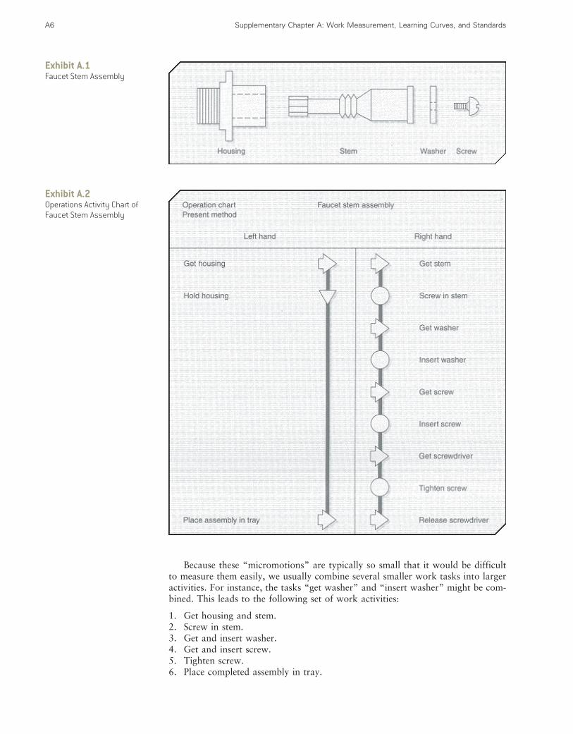
Because these “micromotions” are typically so small that it would be difficultto measure them easily, we usually combine several smaller work tasks into largeractivities. For instance, the tasks “get washer” and “insert washer” might be com-bined. This leads to the following set of work activities:

1. Get housing and stem.2. Screw in stem.3. Get and insert washer.4. Get and insert screw.5. Tighten screw.6. Place completed assembly in tray.


Exhibit A.1Faucet Stem Assembly

Exhibit A.2Operations Activity Chart ofFaucet Stem Assembly

To determine the sample size needed for a time study, suppose we desire a 90percent probability that the value of the sample mean provides a sampling error of.01 minute or less. Further assume that � is estimated from historical experienceto be .019. Therefore, � � .10, z.05 � 1.645, and E � .01. Using Equation (A.3),we compute

n � (1.645)2(.019)2/(.01)2 � 9.8 � 10 observations

A sample size of 10 or more will provide the required precision. (Fractional valuesof n should always be rounded upward to ensure that the precision is at least asgood as desired.)

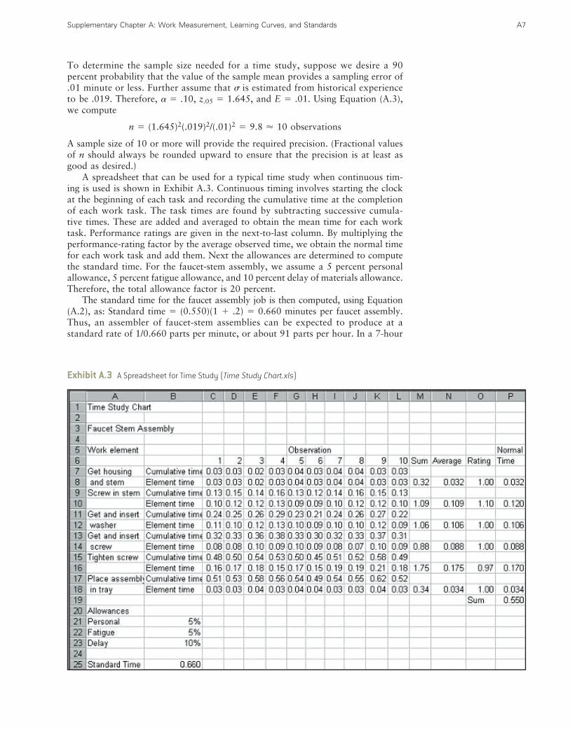
A spreadsheet that can be used for a typical time study when continuous tim-ing is used is shown in Exhibit A.3. Continuous timing involves starting the clockat the beginning of each task and recording the cumulative time at the completionof each work task. The task times are found by subtracting successive cumula-tive times. These are added and averaged to obtain the mean time for each worktask. Performance ratings are given in the next-to-last column. By multiplying theperformance-rating factor by the average observed time, we obtain the normal timefor each work task and add them. Next the allowances are determined to computethe standard time. For the faucet-stem assembly, we assume a 5 percent personalallowance, 5 percent fatigue allowance, and 10 percent delay of materials allowance.Therefore, the total allowance factor is 20 percent.

The standard time for the faucet assembly job is then computed, using Equation(A.2), as: Standard time � (0.550)(1 � .2) � 0.660 minutes per faucet assembly.Thus, an assembler of faucet-stem assemblies can be expected to produce at astandard rate of 1/0.660 parts per minute, or about 91 parts per hour. In a 7-hour


Exhibit A.3 A Spreadsheet for Time Study (Time Study Chart.xls)

workday with 1 hour off for lunch and breaks, an assembler can produce (7)(91) � 637 faucet-stem assemblies per workday.

Using Regression Analysis to Determine Standard TimeRegression analysis provides an alternative method to estimating the time requiredto do a particular job or work activity. Regression analysis is used to predict timesbased on different attributes of the work, rather than by adding up individual tasktimes. Using regression to estimate standard times can be advantageous because itavoids the assumption of additive task times when this might not hold; statisticallysignificant variables can be determined; confidence intervals for the prediction canbe developed; and finally, it may cost less than a detailed work study.

Consider the following problem on developing standard time estimates for in-stalling electrical power lines. An electric power company wishes to determine astandard time-estimating formula for installing power lines. A good formula wouldhelp it plan capacity and staffing needs. The following data are collected:

Total Number Wire No. of No. of No. ofTime (hours) of Poles (100 feet) Cross Arms Insulators Guy wires

8.0 1 4 1 2 114.0 2 10 2 4 017.5 3 6 3 6 17.0 1 2.5 2 3 0

16.0 2 10 4 6 037.5 4 24 8 12 239.5 4 33 7 11 110.5 1 3 2 4 217.0 2 8 4 8 123.5 3 12 6 12 016.5 2 12 2 4 122.0 3 18 3 6 08.5 1 5 2 3 0

28.5 4 12 8 12 0

Exhibit A.4 shows the results using Excel’s Regression tool. The model obtainedfrom this analysis is

Time � 0.237 � 2.804 Poles � 0.514 Wire � 1.09 Cross arms �0.170 Insulators � 1.50 Guy wires

The regression analysis shows a high R2 value, showing a strong fit to the data.Moreover, the p values for the regression coefficients are significant, meaning thateach of the variables contributes to predicting time. If the utility faces a situationin which it estimates installation of 4 poles, 1,500 feet of wire, 7 cross arms, 12insulators, and no guy wires, the predicted time for the job would be

Time � 0.237 � 2.804 � 4 � 0.514 � 1500 � 1.09 � 7 � 0.170 � 12 � 1.50 � 0 � 792 hours

Predetermined Time Standard MethodsPredetermined time standards describe the amount of time necessary to accomplishspecific movements (called micromotions), such as moving a human hand a certaindistance or lifting a 1-pound part. These small time estimates have been documentedand are available in books and electronic tables. If a job, work activity, or task canbe broken down into such elemental tasks, an estimate of the normal time is madeby adding up these predetermined times. This approach is especially appealing fordeveloping standard times for new manufactured goods and some service tasks. An


electronics manufacturer, for example, may have much experience with assemblingsmall electronic components using human labor and keep a record of past micro-motion and normal time analyses. For similar new tasks and electronic componentparts, predetermined time standards can be used to estimate new normal times. Pre-determined time standards were originally developed for labor-intensive humantasks but data sets exist for machine micromovements, such as those involving anautomated drill press.

Predetermined time standards are advantageous since they cost less than a stop-watch time study, avoid needing multiple performance ratings, and are best for newgoods and services. However, this type of micromotion-based time standard is notjustified for small order sizes or infrequent production runs. In addition, once thenew good or service and its associated process are stable and running well, stop-watch or work-sampling time studies still need to be done. Finally, the assumptionof additivity is sometimes questionable, since a process or assembly sequence of dif-ficult versus simple micromotions may or may not be additive.

The Debate Over Work StandardsWork standards evolved at the turn of the twentieth century, and although theyhave supported significant gains in productivity, they have been the subjects ofdebate since the quality revolution began in the United States. Critics such as W. Edwards Deming have condemned work standards on the basis that they destroyintrinsic motivation in jobs and rob workers of the creativity necessary for contin-uous improvement. That is certainly true when managers dictate standards in aneffort to meet numerical goals set up by their superiors. However, the real culpritin that case is not the standards themselves, but managerial style. The old style of


Exhibit A.4 Results of Regression Analysis for Electric Power Line Installation

managing reflects Taylor’s philosophy: Managers and engineers think, and work-ers do what they are told. A total quality approach suggests that empowered work-ers can manage their own processes with help from managers and professional staff.

Experience at GM’s NUMMI plant has shown that work standards can havevery positive results when they are not imposed by dictum, but designed by theworkers themselves in a continuous effort to improve productivity, quality, andskills.3 At the GM-Fremont plant, industrial engineers performed all of the meth-ods analysis and work-measurement activities, designing jobs as they saw fit. Whenthe industrial engineers were performing motion studies, workers would naturallyslow down and make the work look harder. At NUMMI, team members learnedtechniques of work analysis and improvement, then timed one another with stop-watches, looking for the safest, most efficient way to do each task at a sustainablepace. They picked the best performance, broke it down to its fundamental elements,and then explored ways to improve the task. The team compared the analyses withthose from other shifts at the same workstation, and wrote detailed specificationsthat became the work standards. Results were excellent. From a total quality per-spective, this was simply an approach to reduce variability. In addition, safety andquality improved, job rotation became more effective, and flexibility increased.

Work SamplingWork sampling is a method of randomly observing work over a period of time toobtain a distribution of the activities that an individual or a group of employeesperform. Work sampling determines the proportion of time spent doing certainactivities on a job. It can be used to determine the percentage of idle time and alsoas a means of assessing nonproductive time to determine performance ratings orto establish allowances. Work sampling is based on the binomial probability dis-tribution, because it is concerned with the proportion of time that a certain activ-ity occurs. Thus, the sample size (n) for a work-sampling study is found by usingEquation (A.4):

n � (z�/2)2p(1 � p)/E2 (A.4)

where p is an estimate of the population proportion of the binomial distribution.Obviously, p will never be known exactly, since it is the population parameter weare trying to estimate. We can choose a value for p from past data, a preliminarysample, or a subjective estimate. If p is difficult to determine in those ways, we canselect p � 0.5, since it gives us the largest value for p(1 � p) and therefore pro-vides the largest and most conservative sample size.

To illustrate work sampling, consider the secretarial staff in a college depart-ment office. The secretaries spend their time in various ways, such as

1. answering the telephone,2. typing drafts of technical papers,3. revising technical papers,4. talking to students,5. duplicating class handouts,6. other productive activities,7. personal time,8. idle periods.

Suppose that a new voice-activated word processing software could greatly increaseproductivity in typing, spell checking, and revising technical papers. However, thepurchase of this product is not justified unless it is used a significant percentage ofthe time. To determine the percentage of time secretaries spend performing the rel-evant work activities, we could observe them at random times and record their ac-tivities. If 100 observations are taken, we might get the results in Exhibit A.5.


Work sampling is a method of randomly observing workover a period of time toobtain a distribution of theactivities that an individual ora group of employeesperform.


Activity Frequency

Answering the telephone 14Typing drafts 21Revising papers 7Talking to students 10Duplicating 15Other productive activity 25Personal 6Idle 2

Total 100

Exhibit A.5Work Sampling ActivityFrequency Data

Learning ObjectiveTo understand the concept oflearning curves and how they canaffect business decisions, and tolearn computational methods forestimating aggregate productiontimes in learning environments.

The percentage of time spent typing or revising is 21 percent � 7 percent � 28 per-cent. To determine the needed sample size (that is, the number of observations), sup-pose we want to estimate the proportion of time spent typing to �5 percent, witha 95 percent probability. We use Equation (A.4), with E � 0.05 and z�/2 � 1.96.Suppose the head secretary estimates that 40 percent of the time is spent typing. Thisprovides a value for p of 0.4. Then the needed sample size using Equation (A.4) is

n � (1.96)20.4(1 � 0.4)/0.052 � 368.8 or at least 369 observations

If that is to be done over a 1-week (40-hour) period, it represents approximately 9observations per hour (9.225, to be exact). The observations should be taken ran-domly when work is at a normal level (not during the spring break!).

To take a random sample, we can use the table of random digits in Appendix C.There are several ways to use random digits in deciding when to take observations.For this example, an average of 9.225 observations per hour requires the observa-tions to be spaced, on the average (60/9.225) � 6.5 minutes apart. We should nottake observations exactly 6.5 minutes apart, however, for then the sample wouldnot be random. Suppose observations are between 3 and 10 minutes apart. If theyare random, the average is 6.5 minutes. We can use the random digits as follows.Suppose the first observation is taken at 9:00. We choose numbers from the firstrow of Appendix C to find how many minutes later we should take the next obser-vation (0 represents 10 minutes, and we discard any 1s or 2s). For instance, the firstnumber is 6; thus we take the next observation at 9:06. The next number is 3, sothe third observation is made at 9:09. We discard the 2 and take the next observa-tion 7 minutes later, at 9:16. We see that the time and cost required to take a ran-dom sample can be significant; that is one of the disadvantages of random sampling.

Work sampling is based on statistics, and like all statistical procedures, it cansuffer from sampling error and lead to erroneous conclusions simply by chance.Also, as the famous Hawthorne experiments showed, people often change their be-havior when being observed, and this can influence the results. Thus, work sam-pling should be used with caution.

LEARNING CURVESThe learning curve concept is that direct labor unit cost decreases in a predictablemanner as the experience in producing the unit increases. For most people, for ex-ample, the longer they play a musical instrument or a video game, the better andfaster they become. The same is true in assembly operations, which was recognizedin the 1920s at Wright-Patterson Air Force Base in the assembly of aircraft. Studiesshowed that the number of labor hours required to produce the fourth plane wasabout 80 percent of the amount of time spent on the second; the eighth plane took

only 80 percent as much time as the fourth; the sixteenth plane 80 percent of thetime of the eighth, and so on. The decrease in production time as the number pro-duced increases is illustrated in Exhibit A.6. As production doubles from x units to2x units, the time per unit of the 2xth unit is 80 percent of the time of the xth unit.This is called an 80 percent learning curve. Such a curve exhibits a steep initial de-cline and then levels off as employees become more proficient in their tasks. In gen-eral, a p-percent learning curve characterizes a process in which the time of the 2xthunit is p percent of the time of the xth unit.

Defense industries (for example, the aircraft and electronics industries), whichintroduce many new and complex products, use learning curves to estimate laborrequirements and capacity, determine costs and budget requirements, and plan andschedule production. Eighty-percent learning curves are generally accepted as a stan-dard, although the ratio of machine work to manual assembly affects the curve per-centage. Obviously, no learning takes place if all assembly is done by machine. Asa rule of thumb, if the ratio of manual to machine work is 3 to 1 (three-fourthsmanual), then 80 percent is a good value; if the ratio is 1 to 3, then 90 percent isoften used. An even split of manual and machine work would suggest the use ofan 85 percent learning curve. The learning factor may also be estimated from pasthistories of similar parts or products.

Mathematically, the learning curve is represented by the function

y � ax�b (A.5)

where

x � number of units produced,a � hours required to produce the first unit,y � time to produce the xth unit, andb � constant equal to �ln p/ln 2 for a 100p percent learning curve.

Thus, for an 80 percent learning curve, p � 0.8 and

b � �ln 0.8/ln 2 � �(�0.223)/0.693 � 0.322

For a 90 percent curve, p � 0.9 and

b � �ln 0.9/ln 2 � �(�0.105)/0.693 � 0.152

Although the learning curve theory implies that improvement will continue for-ever, in actual practice the learning curve flattens out. As management interest inthe initial creation of a new good or service decreases, employees may reach a level


A p-percent learning curve

characterizes a process inwhich the time of the 2xthunit is p percent of the timeof the xth unit.

The learning curve concept isthat direct labor unit costdecreases in a predictablemanner as the experience inproducing the unit increases.

Exhibit A.6An 80 Percent Learning Curve

of production that is expected of them and hold that rate. Another way to viewthe theory of learning is that early on extraordinary new practices and methodsare found to dramatically improve performance, such as substituting plastic forsteel parts. Later in the life of the learning curve, the focus shifts to incrementalimprovements.

Learning curves can apply to individual employees or, in an aggregate sense, tothe big-picture initiatives such as pricing strategy. For example, learning curves areused to monitor employees typing and encoding checks in a bank’s operations. Eachemployee must reach a certain threshold-learning rate within 6 months or moretraining is required. In some cases, the bank-encoding employee is transferred toanother bank job because the employee is just not suited to the encoding job. Learn-ing curves help managers make such decisions. From an aggregate and strategic per-spective, a firm may use the learning-curve concept to establish a pricing schedulethat does not initially cover cost in order to gain increased market share.

Managers should realize that improvement along a learning curve does not takeplace automatically. Learning-curve theory is most applicable to new products orprocesses that have a high potential for improvement and when the benefits will berealized only when appropriate incentives and effective motivational tools are used.Organizational changes may also have significant effects on learning. Changes intechnology or work methods will affect the learning curve, as will the institutionof productivity and quality-improvement programs.

As an illustration of learning curves, suppose a manufacturing firm is intro-ducing a new and complex machine and has determined that a 90 percent learningcurve is applicable. Estimates of demand for the next 3 years are 50, 75, and 100units. The time to produce the first unit is estimated to be 3,500 hours. Therefore,the learning-curve function is

y � 3,500x�0.152

Consequently, the time to manufacture the second unit will be

3,500 (2)�0.152 � 3,150 hours

Exhibit A.7 gives the cumulative number of hours required to produce the 3-yeardemand in increments of 25 units. Thus, to produce the 50 units in the first year,the firm will require 112,497 hours. If we assume that each employee works 160hours per month, or 1,920 hours per year, we find that for the first year the firmwill need

112,497/1,920 � 59 employees

to produce this machine. In the second year, the total number of hours requiredwill be the difference between the cumulative requirements for the first two years’production (246,160 hours) and the first year’s production (112,497 hours), or

246,160 � 112,497 � 133,663 hours

So the labor requirements for the second year are

133,663 / 1,920 � 70 employees

Similarly, for the third year, the labor requirements are

� 83 employees

These are aggregate numbers; at a more detailed planning level, they will vary ac-cording to how production is actually scheduled over the year. Also, note that thenumber of employees required to produce these units increases in a nonlinear way,

406,112 � 246,160

1,920


reflecting the learning that is taking place among employees. For example, we mightneed 59 employees to produce 50 units, 70 employees for 125, and 83 for 225.Clearly, understanding learning is important for aggregate planning.

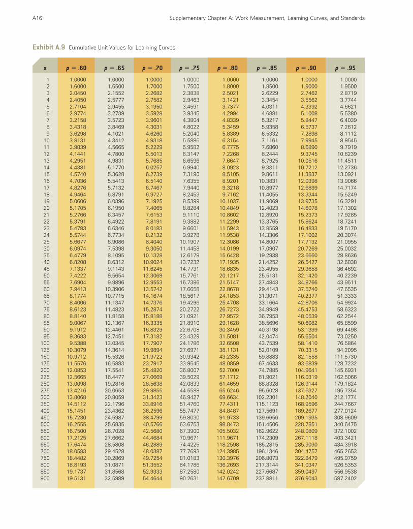
Values for learning-curve functions can be easily computed and summarizedthrough the use of tables. Exhibits A.8 and A.9 present unit values and cumulativevalues, respectively, for learning curves from 60 percent through 95 percent. Tofind the time to produce a specific unit, multiply the time for the first unit by theappropriate factor in Exhibit A.8. For the 90 percent learning-curve example pre-sented earlier, the time for the second unit is 3,500(0.9000) � 3,150. The time forthe third unit is 3,500(0.8462) � 2,961.7, and so on.

To find the time for a cumulative number of units, we can use Exhibit A.9.Thus, for a 90 percent learning curve, if the time for the first unit is 3,500, the timefor the first 25 units is 3,500(17.7132) � 61,996. Similarly, the time for the first100 units is 3,500(58.1410) � 203,494. The values in Exhibit A.7 were found us-ing this table.

A broader extension of the learning curve is the experience curve. The experi-

ence curve states that the cost of doing any repetitive task, work activity, or projectdecreases as the accumulated experience of doing the job increases. The terms im-provement curve, experience curve, and manufacturing progress function are oftenused to describe the learning phenomenon in the aggregate context. Marketing re-search, software design, developing engineering specifications for a water plant, ac-counting and financial auditing of the same client, implementing a softwareintegration project, and so on are examples of this broader view. The idea is thateach time experience doubles, costs decline by 10 percent to 30 percent. Costs mustalways be translated into constant dollars to eliminate the inflation effect. Of course,the learning or experience curve does not continue this dramatic decrease in timeand costs indefinitely, and at some point begins to flatten out.

Practical Issues in Using Learning CurvesThe following ten factors can affect the applicability of the learning or experiencecurve and/or the amount of learning that occurs. Good management judgment isrequired to recognize these factors and take appropriate action, including stoppingthe current learning-curve analysis, beginning a new learning-curve analysis, and/orusing other planning methods for the remainder of the work.

1. The learning curve does not usually apply to supervisory personnel, some skilledcraftspeople, or jobs that have nonrepetitive job tasks.

2. A change in the ratio of indirect labor or supervisory talent to direct labor canalter the rate of learning.

3. The institution of incentive systems, bonus plans, quality initiatives, empower-ment, and the like may increase learning.


Cumulative Units Cumulative Hours Required

25 61,99650 112,49775 159,164

100 203,494125 246,160150 287,545175 327,894200 367,374225 406,112

Exhibit A.7Cumulative Time Required UsingLearning Curves

The experience curve statesthat the cost of doing anyrepetitive task, work activity,or project decreases as theaccumulated experience ofdoing the job increases.


p .60 .65 .70 .75 .80 .85 .90 .95

x b .737 .621 .515 .415 .322 .234 .152 .074

1 1.0000 1.0000 1.0000 1.0000 1.0000 1.0000 1.0000 1.00002 0.6000 0.6500 0.7000 0.7500 0.8000 0.8500 0.9000 0.95003 0.4450 0.5052 0.5682 0.6338 0.7021 0.7729 0.8462 0.92194 0.3600 0.4225 0.4900 0.5625 0.6400 0.7225 0.8100 0.90255 0.3054 0.3678 0.4368 0.5127 0.5956 0.6857 0.7830 0.88776 0.2670 0.3284 0.3977 0.4754 0.5617 0.6570 0.7616 0.87587 0.2383 0.2984 0.3674 0.4459 0.5345 0.6337 0.7439 0.86598 0.2160 0.2746 0.3430 0.4219 0.5120 0.6141 0.7290 0.85749 0.1980 0.2552 0.3228 0.4017 0.4929 0.5974 0.7161 0.8499

10 0.1832 0.2391 0.3058 0.3846 0.4765 0.5828 0.7047 0.843311 0.1708 0.2253 0.2912 0.3696 0.4621 0.5699 0.6946 0.837412 0.1602 0.2135 0.2784 0.3565 0.4493 0.5584 0.6854 0.832013 0.1510 0.2031 0.2672 0.3449 0.4379 0.5480 0.6771 0.827114 0.1430 0.1940 0.2572 0.3344 0.4276 0.5386 0.6696 0.822615 0.1359 0.1858 0.2482 0.3250 0.4182 0.5300 0.6626 0.818416 0.1296 0.1785 0.2401 0.3164 0.4096 0.5220 0.6561 0.814517 0.1239 0.1719 0.2327 0.3085 0.4017 0.5146 0.6501 0.810918 0.1188 0.1659 0.2260 0.3013 0.3944 0.5078 0.6445 0.807419 0.1142 0.1604 0.2198 0.2946 0.3876 0.5014 0.6392 0.804220 0.1099 0.1554 0.2141 0.2884 0.3812 0.4954 0.6342 0.801221 0.1061 0.1507 0.2087 0.2826 0.3753 0.4898 0.6295 0.798322 0.1025 0.1465 0.2038 0.2772 0.3697 0.4844 0.6251 0.795523 0.0992 0.1425 0.1992 0.2722 0.3644 0.4794 0.6209 0.792924 0.0961 0.1387 0.1949 0.2674 0.3995 0.4747 0.6169 0.790425 0.0933 0.1353 0.1908 0.2629 0.3548 0.4701 0.6131 0.788030 0.0815 0.1208 0.1737 0.2437 0.3346 0.4505 0.5963 0.777535 0.0728 0.1097 0.1605 0.2286 0.3184 0.4345 0.5825 0.768740 0.0660 0.1010 0.1498 0.2163 0.3050 0.4211 0.5708 0.761145 0.0605 0.0939 0.1410 0.2060 0.2936 0.4096 0.5607 0.754550 0.0560 0.0879 0.1336 0.1972 0.2838 0.3996 0.5518 0.748655 0.0522 0.0829 0.1272 0.1895 0.2753 0.3908 0.5438 0.743460 0.0489 0.0785 0.1216 0.1828 0.2676 0.3829 0.5367 0.738665 0.0461 0.0747 0.1167 0.1768 0.2608 0.3758 0.5302 0.734270 0.0437 0.0713 0.1123 0.1715 0.2547 0.3693 0.5243 0.730275 0.0415 0.0683 0.1084 0.1666 0.2491 0.3634 0.5188 0.726580 0.0396 0.0657 0.1049 0.1622 0.2440 0.3579 0.5137 0.723185 0.0379 0.0632 0.1017 0.1582 0.2393 0.3529 0.5090 0.719890 0.0363 0.0610 0.0987 0.1545 0.2349 0.3482 0.5046 0.716895 0.0349 0.0590 0.0960 0.1511 0.2308 0.3438 0.5005 0.7139

100 0.0336 0.0572 0.0935 0.1479 0.2271 0.3397 0.4966 0.7112125 0.0285 0.0498 0.0834 0.1348 0.2113 0.3224 0.4800 0.6996150 0.0249 0.0444 0.0759 0.1250 0.1993 0.3089 0.4669 0.6902175 0.0222 0.0404 0.0701 0.1172 0.1896 0.2979 0.4561 0.6824200 0.0201 0.0371 0.0655 0.1109 0.1816 0.2887 0.4469 0.6757225 0.0185 0.0345 0.0616 0.1056 0.1749 0.2809 0.4390 0.6698250 0.0171 0.0323 0.0584 0.1011 0.1691 0.2740 0.4320 0.6646275 0.0159 0.0305 0.0556 0.0972 0.1639 0.2680 0.4258 0.6599300 0.0149 0.0289 0.0531 0.0937 0.1594 0.2625 0.4202 0.6557350 0.0133 0.0262 0.0491 0.0879 0.1517 0.2532 0.4105 0.6482400 0.0121 0.0241 0.0458 0.0832 0.1453 0.2454 0.4022 0.6419450 0.0111 0.0224 0.0431 0.0792 0.1399 0.2387 0.3951 0.6363500 0.0103 0.0210 0.0408 0.0758 0.1352 0.2329 0.3888 0.6314550 0.0096 0.0198 0.0389 0.0729 0.1312 0.2278 0.3832 0.6269600 0.0090 0.0188 0.0372 0.0703 0.1275 0.2232 0.3782 0.6229650 0.0085 0.0179 0.0357 0.0680 0.1243 0.2190 0.3736 0.6192700 0.0080 0.0171 0.0344 0.0659 0.1214 0.2152 0.3694 0.6158750 0.0076 0.0163 0.0332 0.0641 0.1187 0.2118 0.3656 0.6127800 0.0073 0.0157 0.0321 0.0624 0.1163 0.2086 0.3620 0.6098850 0.0069 0.0151 0.0311 0.0508 0.1140 0.2057 0.3587 0.6070900 0.0067 0.0146 0.0302 0.0594 0.1119 0.2029 0.3556 0.6045

Exhibit A.8Unit Values for Learning Curves


Exhibit A.9 Cumulative Unit Values for Learning Curves

x p � .60 p � .65 p � .70 p � .75 p � .80 p � .85 p � .90 p � .95

1 1.0000 1.0000 1.0000 1.0000 1.0000 1.0000 1.0000 1.00002 1.6000 1.6500 1.7000 1.7500 1.8000 1.8500 1.9000 1.95003 2.0450 2.1552 2.2682 2.3838 2.5021 2.6229 2.7462 2.87194 2.4050 2.5777 2.7582 2.9463 3.1421 3.3454 3.5562 3.77445 2.7104 2.9455 3.1950 3.4591 3.7377 4.0311 4.3392 4.66216 2.9774 3.2739 3.5928 3.9345 4.2994 4.6881 5.1008 5.53807 3.2158 3.5723 3.9601 4.3804 4.8339 5.3217 5.8447 6.40398 3.4318 3.8469 4.3031 4.8022 5.3459 5.9358 6.5737 7.26129 3.6298 4.1021 4.6260 5.2040 5.8389 6.5332 7.2898 8.1112

10 3.8131 4.3412 4.9318 5.5886 6.3154 7.1161 7.9945 8.954511 3.9839 4.5665 5.2229 5.9582 6.7775 7.6860 8.6890 9.791912 4.1441 4.7800 5.5013 6.3147 7.2268 8.2444 9.3745 10.623913 4.2951 4.9831 5.7685 6.6596 7.6647 8.7925 10.0516 11.451114 4.4381 5.1770 6.0257 6.9940 8.0923 9.3311 10.7212 12.273615 4.5740 5.3628 6.2739 7.3190 8.5105 9.8611 11.3837 13.092116 4.7036 5.5413 6.5140 7.6355 8.9201 10.3831 12.0398 13.906617 4.8276 5.7132 6.7467 7.9440 9.3218 10.8977 12.6899 14.717418 4.9464 5.8791 6.9727 8.2453 9.7162 11.4055 13.3344 15.524919 5.0606 6.0396 7.1925 8.5399 10.1037 11.9069 13.9735 16.329120 5.1705 6.1950 7.4065 8.8284 10.4849 12.4023 14.6078 17.130221 5.2766 6.3457 7.6153 9.1110 10.8602 12.8920 15.2373 17.928522 5.3791 6.4922 7.8191 9.3882 11.2299 13.3765 15.8624 18.724123 5.4783 6.6346 8.0183 9.6601 11.5943 13.8559 16.4833 19.517024 5.5744 6.7734 8.2132 9.9278 11.9538 14.3306 17.1002 20.307425 5.6677 6.9086 8.4040 10.1907 12.3086 14.8007 17.7132 21.095530 6.0974 7.5398 9.3050 11.4458 14.0199 17.0907 20.7269 25.003235 6.4779 8.1095 10.1328 12.6179 15.6428 19.2938 23.6660 28.863640 6.8208 8.6312 10.9024 13.7232 17.1935 21.4252 26.5427 32.683845 7.1337 9.1143 11.6245 14.7731 18.6835 23.4955 29.3658 36.469250 7.4222 9.5654 12.3069 15.7761 20.1217 25.5131 32.1420 40.223955 7.6904 9.9896 12.9553 16.7386 21.5147 27.4843 34.8766 43.951160 7.9413 10.3906 13.5742 17.6658 22.8678 29.4143 37.5740 47.653565 8.1774 10.7715 14.1674 18.5617 24.1853 31.3071 40.2377 51.333370 8.4006 11.1347 14.7376 19.4296 25.4708 33.1664 42.8706 54.992475 8.6123 11.4823 15.2874 20.2722 26.7273 34.9949 45.4753 58.632380 8.8140 11.8158 15.8188 21.0921 27.9572 36.7953 48.0539 62.254485 9.0067 12.1367 16.3335 21.8910 29.1628 38.5696 50.6082 65.859990 9.1912 12.4461 16.8329 22.6708 30.3459 40.3198 53.1399 69.449895 9.3683 12.7451 17.3182 23.4329 31.5081 42.0474 55.6504 73.0250

100 9.5388 13.0345 17.7907 24.1786 32.6508 43.7539 58.1410 76.5864125 10.3079 14.3614 19.9894 27.6971 38.1131 52.0109 70.3315 94.2095150 10.9712 15.5326 21.9722 30.9342 43.2335 59.8883 82.1558 111.5730175 11.5576 16.5883 23.7917 33.9545 48.0859 67.4633 93.6839 128.7232200 12.0853 17.5541 25.4820 36.8007 52.7000 74.7885 104.9641 145.6931225 12.5665 18.4477 27.0669 39.5029 57.1712 81.9021 116.0319 162.5066250 13.0098 19.2816 28.5638 42.0833 61.4659 88.8328 126.9144 179.1824275 13.4216 20.0653 29.9855 44.5588 65.6246 95.6028 137.6327 195.7354300 13.8068 20.8059 31.3423 46.9427 69.6634 102.2301 148.2040 212.1774350 14.5112 22.1796 33.8916 51.4760 77.4311 115.1123 168.9596 244.7667400 15.1451 23.4362 36.2596 55.7477 84.8487 127.5691 189.2677 277.0124450 15.7230 24.5987 38.4799 59.8030 91.9733 139.6656 209.1935 308.9609500 16.2555 25.6835 40.5766 63.6753 98.8473 151.4506 228.7851 340.6475550 16.7500 26.7028 42.5680 67.3900 105.5032 162.9622 248.0809 372.1002600 17.2125 27.6662 44.4684 70.9671 111.9671 174.2309 267.1118 403.3421650 17.6474 28.5808 46.2889 74.4225 118.2598 185.2815 285.9030 434.3918700 18.0583 29.4528 48.0387 77.7693 124.3985 196.1346 304.4757 465.2653750 18.4482 30.2869 49.7254 81.0183 130.3976 206.8073 322.8479 495.9759800 18.8193 31.0871 51.3552 84.1786 136.2693 217.3144 341.0347 526.5353850 19.1737 31.8568 52.9333 87.2580 142.0242 227.6687 359.0497 556.9538900 19.5131 32.5989 54.4644 90.2631 147.6709 237.8811 376.9043 587.2402

4. Changes in product design, raw material usage, technology, and/or the processmay significantly alter the learning curve.

5. Humans learn simple task(s) quickly and reach a limit on learning for the task(s),but for complex intellectual task(s) such as software programming, learning isless limited and may continue. The first type of learning is described with anexponential curve; the more complex learning is sometimes described by an S-shaped curve.

6. A contract phaseout may result in a lengthening of processing times for the lastunits produced, since employees want to prolong their income period.

7. The lack of proper maintenance of tools and equipment, the nonreplacement oftools, or the aging of equipment can have a negative impact on learning.

8. Keeping groups of employees together, such as highly specialized consultinggroups, reaps a productivity benefit but may stifle innovation and new experi-ences.

9. The transfer of employees may result in an interruption or a regression to anearlier stage of the learning curve or may necessitate a new learning curve.

10. Learning curves focus on direct labor and ignore indirect labor that also con-tributes to efficiency and effectiveness.


SOLVED PROBLEMS

SOLVED PROBLEM #1

Assume your first job out of school is as a branchmanager for a major bank. Your branch also has a back-office operation where bank packs of $300 are assem-bled for retail businesses. Each bank pack contains two$20 bills, ten $10 bills, twelve $5 bills, and one hun-dred $1 bills. Retail customers become upset when thesebank packs are not available since they usually pickthem up before their retail store opens. A continuousstopwatch study collected the information shown in thetable below. The policy of the bank is to use a 20 per-cent allowance factor for branch bank operations. (a)What is the normal and standard time for a bank pack?(b) How long would it take to pack 200 packs? Now

you must decide how many branch bank staff to assignto this work activity and when they will do the work.

Solution:

a. To determine the normal and standard times, notethat the continuous stopwatch study timed eachdenomination separately and the cumulative timesare shown across each row. The “Difference” rowsshow the individual times.

b. (200 bank packs)(31.426 minutes)/10 bank packs� (20)(31.426 minutes) � 628.5 minutes or 10.5 hours

Observation Cycles (cumulative, in minutes) Performance NormalWork Task 1 2 3 4 5 6 7 8 9 Average Rating Time

Count 2 $20s 0.11 0.15 0.36 0.5 0.65 0.78 0.89 1.02 1.22Difference 0.11 0.21 0.14 0.15 0.13 0.11 0.13 0.20 0.15 1.15 0.170Count 10 $10s 0.25 0.66 0.94 1.27 1.79 2.05 2.36 2.77 3.20Difference 0.25 0.28 0.33 0.52 0.26 0.31 0.41 0.43 0.35 0.95 0.331Count 12 $5s 0.37 0.79 0.93 1.44 1.91 2.30 2.88 3.61 4.22Difference 0.37 0.14 0.51 0.47 0.39 0.58 0.73 0.61 0.48 1.00 0.475Count 100 $1s 1.02 2.44 3.70 5.01 6.39 8.11 9.43 10.55 11.55Difference 1.02 1.26 1.31 1.38 1.72 1.32 1.12 1.00 1.27 1.10 1.393Place Bank Packs in Tray (once every ten cycles) � 2.50 1.00

Normal processing (run) time per bank pack � 2.369Normal time per ten bank packs with setup � 26.188

Standard time per bank pack � Normal time � (1 � Allowances) � 2.8426Standard time per ten bank packs with setup � 31.426


SOLVED PROBLEM #2

In a work-sampling study an administrative assistantwas found to be working 2,700 times in a total of 3,000observations made over a time span of 240 workinghours. The employee’s output was 1,800 forms. If a per-formance rating of 1.05 and an allowance of 15 per-cent are given, what is the standard output for this task?

Solution:

Effective number of hours worked � 2,700(240)/3,000� 216.

Output during this period � 1,800 forms.Actual time per form � 216(60)/1,800 � 7.2 minutes,

or 8.33 forms per hour.Normal time � Actual observed time � Performance

rating � 7.2(1.05) � 7.56 minutes.Standard time � 7.56(1.15) � 8.694 minutes per

form.Standard output � 60/8.694 � 6.9 forms per hour,

or 55 forms per 8-hour day.

SOLVED PROBLEM #3

A yacht manufacturer has been commissioned to buildfive sailboats for a Florida resort. The first boat took6,000 labor-hours to build. How many labor-hours willit take to complete the order, assuming that a 90 per-cent learning curve is applicable?

Solution:

Using a 90 percent learning curve, we have the timeslisted here:

Unit Time Required

1 6,0002 5,4003 5,0774 4,8605 4,698

Total 26,035 hours

Or, using Exhibit A.9, 6,000(4.3392) � 26,035 hours.

KEY TERMS AND CONCEPTS

Allowance factorExperience curveLearning curveNormal timeOperations activity chartPerformance rating factorPredetermined time standards

Regression methodSample-size computationsStandard timeTasks and work activitiesTime-study methodWork measurementWork-sampling method

QUESTIONS FOR REVIEW AND DISCUSSION

1. What is work measurement? How can it be used toimprove organizational performance?

2. Explain the concept of normal time. How can anoperations manager verify whether the time to per-form a task is indeed “normal”?

3. How does standard time differ from normal time?How are standard times used in operations man-agement?

4. Do you think the following jobs require standardtimes? Explain your reasoning.

a. Carpet installersb. Software programmersc. Cable T.V. installersd. Hotel maidse. Bank tellersf. Airline flight attendants


g. Dentistsh. Medical doctorsi. Restaurant reservationsj. Telephone call center representatives

5. Explain how regression analysis can be used to es-tablish standard times.

6. Select one of the jobs in Question 4 and describewhat data are needed to use regression analysis todevelop normal times.

7. What is time study? Describe the basic procedurefor conducting a time study.

8. How do predetermined time standards differ fromthose found through a stopwatch time study?

9. Why are work standards the subject of much de-bate? Do some research into arguments and issuesraised by unions to provide an additional basis foryour response.

10. If you have worked for an organization that usedtime standards, provide a short description of howit was used or affected your work. What were thepros and cons of the job and working under stan-dard times? Where the times accurate? How werethey determined?

11. Explain work sampling. Discuss some applicationsof work sampling in both manufacturing and ser-vice organizations.

12. Explain the concept of learning curves. Why are theyimportant in managing operations?

13. What types of jobs are best suited to the applicationof learning curves? How would you determine this?

14. What is the experience curve and how does it differfrom the traditional learning curve?

15. Discuss some practical issues that managers mustconsider in using learning curves.

PROBLEMS AND ACTIVITIES

1. What sample sizes should be used for these timestudies?a. There should be a .95 probability that the value

of the sample mean is within 2 minutes, giventhat the standard deviation is 4 minutes.

b. There should be a 90 percent chance that thesample mean has an error of 0.10 minutes orless when the variance is estimated as 0.50 min-utes.

2. Compute the number of observations required in awork-sampling study if the standard deviation is 0.2minute and there should be a 90 percent chance thatthe sample mean has an error of (a) 0.15 minute,(b) 0.10 minute, and (c) 0.005 minute.

3. In a work-sampling study, what sample size shouldbe used to provide 95 percent probability that the

processing time of a single order form has an errorof 0.05 minute? There is no estimate of the clericalstaff’s proportion of productive time.

4. Exhibit A.10 shows a partially completed time-studyworksheet. Determine the standard time for this op-eration.

5. Using a rating factor of 1.00, compute the normaltime for drilling a hole in a steel plate if these arethe observed times (in minutes):

0.24 0.25 0.29 0.24 0.270.25 0.245 0.19 0.20 0.23

6. Using a fatigue allowance of 20 percent, and giventhe following time-study data obtained by continu-ous time measurement, compute the standard time.

Table for Problem 6.

Cycle of ObservationActivity 1 2 3 4 5 Performance Rating

Get casting 0.21 2.31 4.41 6.45 8.59 0.95Fix into fixture 0.48 2.59 4.66 6.70 8.86 0.90Drilling operation 1.52 3.65 5.66 7.74 9.90 1.00Unload 1.73 3.83 5.91 7.96 10.10 0.95Inspect 1.98 4.09 6.15 8.21 10.30 0.80Replace 2.10 4.20 6.25 8.34 10.42 1.10


Exhibit A.10 Time Study Worksheet for Problem 4

Time Study ChartNormal

Work element 1 2 3 4 5 6 7 8 9 Sum Avg Rating time

ACumulative time .09 .12 .06 .11 .10 .09 .13 .12 .13

1.05Element time

BCumulative time .23 .28 .21 .20 .24 .22 .26 .25 .25

1.00Element time

CCumulative time .46 .49 .46 .44 .47 .47 .49 .46 .48

.90Element time

DCumulative time .61 .66 .62 .59 .69 .67 .67 .66 .70

.85Element time

ECumulative time .70 .74 .72 .68 .79 .80 .76 .78 .81

1.00Element time

FCumulative time 1.00 1.02 .98 .99 1.07 1.09 1.02 1.06 1.09

1.10Element time

Allowances: Personal 5% Standard Time __________Sum

Fatigue 5%Delay 5%

7. Provide the data missing from the following infor-mation. Time is in minutes.

Actual Normal Standard Performance FatigueTime Time Time Rating Allowance

10.6 _____ _____ 1.06 20%7.8 7.2 _____ _____ 15%6.5 _____ 7.98 1.05 _____2 _____ _____ 1.10 15%

8. A part-time employee who rolls out dough balls ata pizza restaurant was observed over a 40-hourperiod for a work-sampling study. During that time,she prepared 550 pieces of pizza dough. The ana-lyst made 50 observations and found the employeenot working four times. The overall performancerating was 1.10. The allowance for the job is 15 per-cent. Based on these data, what is the standard timein minutes for preparing pizza dough?

9. How many observations should be made in a work-sampling study to obtain an estimate within 10 per-cent of the proportion of time spent changing tools bya production worker with a 99 percent probability?

10. Operating at an 80 percent learning rate, the firstunit took 72 hours to produce. How long will the32nd unit take?

11. Linda Bryant recently started a small home-construction company. In an effort to foster highquality, rather than subcontracting individual work,she has formed teams of employees who are re-sponsible for the entire job. She has contracted witha developer to build 20 homes of similar type andsize. She has four teams of workers. The first homeswere built in an average of 145 days. How long willit take to complete the contract if an 85 percentlearning curve applies?

12. Suppose a manufacturer of copiers has concludedthat a 75 percent learning curve applies to the timea beginning service technician takes to install copymachines. If the time required to install the first copymachine is estimated to be 4 hours, what is an esti-mate of the time required by a new technician to in-stall the second and third copiers?

13. A manufacturer has committed to supply 16 unitsof a particular product in 4 months (that is, 16weeks) at a price of $30,000 each. The first unittook 1,000 hours to produce. Even though the sec-ond unit took only 750 hours to produce, the man-ufacturer is anxious to know:

a. if the delivery commitment of 16 weeks will bemet,

b. whether enough labor is available (currently 500hours are available per week),

c. whether or not the venture is profitable.

Apply learning-curve theory to each of those issues.Assume the material cost per unit equals $22,000;labor equals $10 per labor-hour, and overhead is$2,000 per week.


CASES

REHABILITATION HOSPITAL OF FLORIDA

A rehabilitation hospital in Florida is having troubleretaining physical therapists. The lack of an employeereward and recognition system and too high a work-load are the top two reasons for the therapists leaving.The hospital currently has no productivity measurementsystem, and compensation is not based on standardizedrequirements or performance. Out-of-date historicaldata have been used to estimate the time per patienttype each physical therapist should spend with eachpatient. These values are: head trauma patients—1.09hours/session, spinal cord injury—1.53 hours/session,and general rehabilitation—0.62 hour. No informationwas available on the patient mix.

Stopwatch-based time studies were performed foreach of the three patient categories with 24 therapists over

a 2-month period. The normal times were determinedto be as follows: head trauma—1.24 hours/session,spinal cord injury—2.03 hours/session, and generalrehabilitation—0.93 hour. The hospital decided to usethese revised normal times to plan its staffing levels andincentive system.

Explain the implications of the lack of a good pro-ductivity measurement system on the hospital’s opera-tions management activities. How might the time-studyinformation be used effectively? What other informa-tion would you want to know to conduct this time studybetter and possibly compute the benefits and costs ofusing the revised standard times?

THE STATE VERSUS JOHN BRACKET4

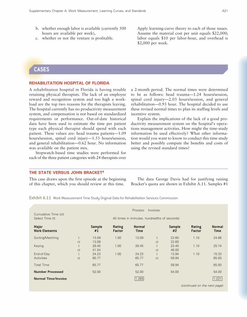
This case draws upon the first episode at the beginningof this chapter, which you should review at this time.

The data George Davis had for justifying raisingBracket’s quota are shown in Exhibit A.11. Samples #1

Exhibit A.11 Work Measurement Time Study Original Data for Rehabilitation Services Commission

Process: InvoicesCumulative Time (ct)Select Time (t) All times in (minutes. hundredths of seconds)

Major Sample Rating Normal Sample Rating NormalWork Elements #1 Factor Time #2 Factor Time

Sorting/Matching t 13.09 1.00 13.09 t 22.60 1.10 24.86ct 13.09 ct 22.60

Keying t 28.45 1.00 28.45 t 23.40 1.10 25.74ct 41.54 ct 46.00

End-of-Day t 24.23 1.00 24.23 t 13.94 1.10 15.33Activities ct 65.77 65.77 ct 59.94 65.93

Total Time 65.77 65.77 59.94 65.93

Number Processed 52.00 52.00 54.00 54.00

Normal Time/Invoice 1.265 1.221

(continued on the next page)


to #4 represent four different commission employeesdoing the same job as Bracket—processing commissioninvoices. These data result in an average normal timeper invoice of 1.0915 minutes [(1.265 � 1.221 � 1.003� 0.877)/4]. With an allowance factor of 20 percent,the standard time is 1.3098 (1.0915 � 1.2) minutes perinvoice, or 45.81 per hour. During a typical 7-hourworkday, an average employee could process 320.66invoices per day, assuming a 1-hour lunch break.

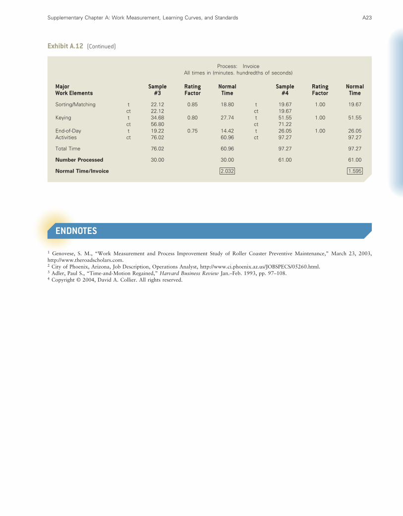
A similar study was performed for Bracket’s invoice-processing productivity; these results are shown in Ex-hibit A.12. These data result in an average normal timeper invoice of 1.722 minutes [(1.808 � 1.452 � 2.032

� 1.595)/4]. With an allowance factor of 20 percent,the standard time is 2.066 (1.722 � 1.2) minutes perinvoice, or 29.04 per hour. During a typical 7-hourworkday, Bracket could process 203.29 invoices perday, assuming a 1-hour lunch break.

a. Whose case is justified—Davis or Bracket? Explain.

b. What other issues should be considered?

c. Would you present these data in court? Why or whynot?

d. What are your final recommendations?

Exhibit A.11 (Continued)

Process: InvoicesAll times in (minutes. hundredths of seconds)



Keying t 14.26 1.10 15.69 t 5.55 1.20 6.66ct 22.70 ct 12.98


Total Time 29.17 32.09 28.50 34.20



Exhibit A.12 Work Measurement Time Study Original Data for John Bracket

Process: InvoiceCumulative Time (ct)Select Time (t) All times in (minutes. hundredths of seconds)



Keying t 23.92 0.80 19.14 t 27.86 0.90 25.07ct 49.50 ct 43.55


Total Time 56.50 45.20 52.51 46.47



(continued on the next page)


ENDNOTES

1 Genovese, S. M., “Work Measurement and Process Improvement Study of Roller Coaster Preventive Maintenance,” March 23, 2003,http://www.theroadscholars.com.2 City of Phoenix, Arizona, Job Description, Operations Analyst, http://www.ci.phoenix.az.us/JOBSPECS/05260.html.3 Adler, Paul S., “Time-and-Motion Regained,” Harvard Business Review Jan.–Feb. 1993, pp. 97–108.4 Copyright © 2004, David A. Collier. All rights reserved.

Exhibit A.12 (Continued)

Process: InvoiceAll times in (minutes. hundredths of seconds)



Keying t 34.68 0.80 27.74 t 51.55 1.00 51.55ct 56.80 ct 71.22


Total Time 76.02 60.96 97.27 97.27



Documents

SUPPLEMENTARY Work Measurement, Learning … Outline Work Measurement OM Spotlight: Work Measurement Activities in Roller Coaster Maintenance Time Study Methods OM Spotlight: Job Description—