Ann Oper ResDOI 10.1007/s10479-013-1522-1

Supply chain scheduling to minimize holding costswith outsourcing

Esaignani Selvarajah · Rui Zhang

© Springer Science+Business Media New York 2014

Abstract This paper addresses a scheduling problem in a flexible supply chain, in whichthe jobs can be either processed in house, or outsourced to a third-party supplier. The goalis to minimize the sum of holding and delivery costs. This problem is proved to be stronglyNP-hard. Consider two special cases, in which the jobs have identical processing times. Forthe problem with limited outsourcing budgets, a NP-hardness proof, a pseudo-polynomialalgorithm and a fully polynomial time approximation scheme are presented. For the problemwith unlimited outsourcing budgets, the problem is shown to be equivalent to the shortestpath problem, and therefore it is in class P . This shortest-path-problem solution approachis further shown to be applicable to a similar but more applicable problem, in which thenumber of deliveries is upper bounded.

Keywords Supply chain scheduling · Outsourcing · Inventory control · FPTAS ·Approximation algorithm · Shortest path problem

1 Introduction

Supply chain management has been one of the most important topics in manufacturingresearch. According to the survey paper (Thomas and Griffin 1996), over 11 % of theU.S. Gross National Product is spent on logistics. This underlines the need for researchdealing with supply chain problems on the operational level using deterministic models.Hall and Potts (2003) conduct exclusive studies on a series of supply chain schedulingproblems, where batch-delivery costs are considered as part of objectives. Similar topicsin this research area can be seen in the follow-up papers, (Chen and Vairaktarakis 2005;

This research was supported in part by NSERC Discovery Grant 1798-03.

E. Selvarajah · R. Zhang (B)Odette School of Business, University of Windsor, 401 Sunset Avenue, Windsor N9B 3P4, ON, Canadae-mail: zhangr6@mcmaster.ca

E. Selvarajahe-mail: selvare@uwindsor.ca

Ann Oper Res

Agnetis et al. 2006; Chen and Hall 2007; Wang and Cheng 2009). More supply chainscheduling problems with a variety of delivery options and their solution approaches arereviewed by Chen (2010).

Considering an in-house production system, a job’s completion time is defined as thetime when the job is ready to leave the system (or get delivered to customers). Let a jobbe in the system from time 0. Then, the job’s weighted completion time can be interpretedas its holding cost. Due to the fact that delivery costs are usually associated with transfer-ring jobs from production systems to customers, jobs are delivered in batches in order tosave delivery costs while making sure that the holding costs due to waiting for deliveries donot cancel the savings from batch-deliveries. Hall and Potts (2003) first introduced supplychain scheduling problems of minimizing the total weighted completion times (i.e., holdingcosts) and delivery costs on a single machine, which reflect the trade-off between inboundmanufacturing and outbound logistics scheduling. Selvarajah and Steiner (2009) and Sel-varajah et al. (2011) study similar problems, where jobs are available sequentially, obtaininga 1.5-approximation algorithm and a meta-genetic heuristic, respectively.

Over the last several decades, an increasing number of suppliers intend to coordinate withoutsourcing partners (or third-party suppliers), when they don’t have sufficient productioncapacity. For example, if a supplier cannot get some order (or job) done due to its limitedproduction capacity, the supplier may subcontract part of the job to a third-party supplierrather than expand its own production capacity. In this case, the supplier needs to processonly the un-subcontracted part of the job. In scheduling, this can be modeled by control-lable processing times. For more details in this topic, the readers are referred to the surveypaper (Shabtay and Steiner 2007). As an extreme case, a job’s processing time can be eitherreduced to zero (outsource the whole job to a third-party supplier), or kept as the origin (pro-cess the whole job in house). In scheduling, this is called scheduling with rejection. Engelset al. (2003) study single machine scheduling problems of minimizing the total weightedcompletion times with rejection. In the paper, they present a pseudo-polynomial algorithmand a fully polynomial time approximation scheme (FPTAS) for the problem.

Our problem is the batching version of the problem in Engels et al. (2003), in whichboth limited and unlimited outsourcing (or rejection) budgets are considered. The unlimited-budget setting simply reflects suppliers’ efforts to maximize profits (or minimize total costs).However, due to two major disadvantages of outsourcing: concerns of loss of control andissues with confidentiality and security, outsourcing budget might be limited or even set tozero. In private sectors, suppliers may not want to outsource any of their core competencies.In this case, if outsourcing has to be conducted, the budget is upper bounded. In publicsectors, it may be more restricted, e.g., by McKenna Long and Aldridge (2004), “(The) 2004Consolidated Appropriations Act contains a provision which limits federal contractors whowin outsourced (US) federal contracts from performing the work overseas”.

As a new emerging area, scheduling with outsourcing attracts more and more attentionsfrom scheduling researchers. Steiner and Zhang (2011) present a pseudo-polynomial algo-rithm and an FPTAS for the single machine scheduling problem of minimizing the totaltardiness, due-date-assignment and rejection costs. However, this paper does not includebatching or delivery costs. Qi (2008) study several scheduling measures with outsourcingand logistics coordination. In this paper, the outsourced jobs are required to be sent back tothe supplier, and delivered to customers together with the jobs processed in house. However,this paper has unlimited outsourcing budgets. Zhang et al. (2010) propose an NP-hardnessproof, a pseudo-polynomial and an approximation algorithm for the scheduling problem ofminimizing the makespan with limited outsourcing budgets. More models and results in thisresearch area can be found in the review paper (Shabtay et al. 2013).

Ann Oper Res

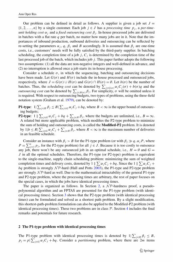
Our problem can be defined in detail as follows. A supplier is given a job set J ={1,2, . . . , n} by a single customer. Each job j ∈ J has a processing time pj , a per-time-unit holding cost αj and a fixed outsourcing cost βj . In-house processed jobs are deliveredin batches with a flat rate q per batch, no matter how many jobs are in it. Note that the im-portances of inbound production, outbound deliveries and outsourcing can be reflected byre-setting the parameters αj , q , βj and B accordingly. It is assumed that βj are one-timecosts, i.e., customers’ needs will be fully satisfied by the third-party supplier. In batchingscheduling, the completion time of a job j , Cj is determined by the completion time of thelast processed job of the batch, which includes job j . This paper further adopts the followingtwo assumptions: (1) all the data are non-negative integers and well-defined in advance, and(2) no interruption is allowed once a job starts its in-house processing.

Consider a schedule σ , in which the sequencing, batching and outsourcing decisionshave been made. Let G(σ) and H(σ) include the in-house processed and outsourced jobs,respectively, where J = G(σ) ∪ H(σ) and G(σ) ∩ H(σ) = ∅. Let b(σ ) be the number ofbatches. Thus, the scheduling cost can be denoted by

∑j∈G(σ) αjCj (σ ) + b(σ )q and the

outsourcing cost can be denoted by∑

j∈H(σ) βj . For simplicity, σ will be omitted unless itis required. With respect to outsourcing budgets, two types of problems, using the three-fieldnotation system (Graham et al. 1979), can be denoted by:

P1-type: 1|∑j∈H βj ≤ B|∑j∈G αjCj +bq , where B < ∞ is the upper bound of outsourc-ing budgets;

P2-type: 1 ‖ ∑j∈G αjCj + bq + ∑

j∈H βj , where the budgets are unlimited, i.e., B = ∞.A related but more applicable problem, which modifies the P2-type problem to minimizethe sum of holding and outsourcing costs, is called the Modified-P2 problem. It is denotedby 1|b ≤ R|∑j∈G αjCj + ∑

j∈H βj , where R < ∞ is the maximum number of deliveriesin an feasible schedule.

Consider an instance with βj > B for the P1-type problem (or with βj q,αjP , whereP = ∑n

j=1 pj , for the P2-type problem) for all j ∈ J . Because it is too costly to outsourceany job, there won’t be any outsourced job in an optimal schedule, i.e., H = ∅ and G =J in all the optimal schedules. Therefore, the P1-type (or P2-type) problem is equivalentto the single-machine, supply chain scheduling problem: minimizing the sum of weightedcompletion times and delivery costs, denoted by 1 ‖ ∑

αjCj + bq . Since the 1 ‖ ∑αjCj +

bq problem is strongly NP-hard (Hall and Potts 2003), the P1-type and P2-type problemare strongly NP-hard as well. Due to the mathematical intractability of the general P1-typeand P2-type problem, where the processing times are arbitrary, the rest of paper focuses onthe special cases, in which the jobs have identical processing times.

The paper is organized as follows. In Section 2, a NP-hardness proof, a pseudo-polynomial algorithm and an FPTAS are presented for the P1-type problem (with identi-cal processing times). Section 3 shows that the P2-type problem (with identical processingtimes) can be formulated and solved as a shortest path problem. By a slight modification,this shortest-path-problem formulation can also be applied to the Modified-P2 problem (withidentical processing times). These two problems are in class P . Section 4 includes the finalremarks and potentials for future research.

2 The P1-type problem with identical processing times

The P1-type problem with identical processing times is denoted by 1|∑j∈H βj ≤ B ,pj = p|∑j∈G αjCj + bq . Consider a partitioning problem, where there are 2m items

Ann Oper Res

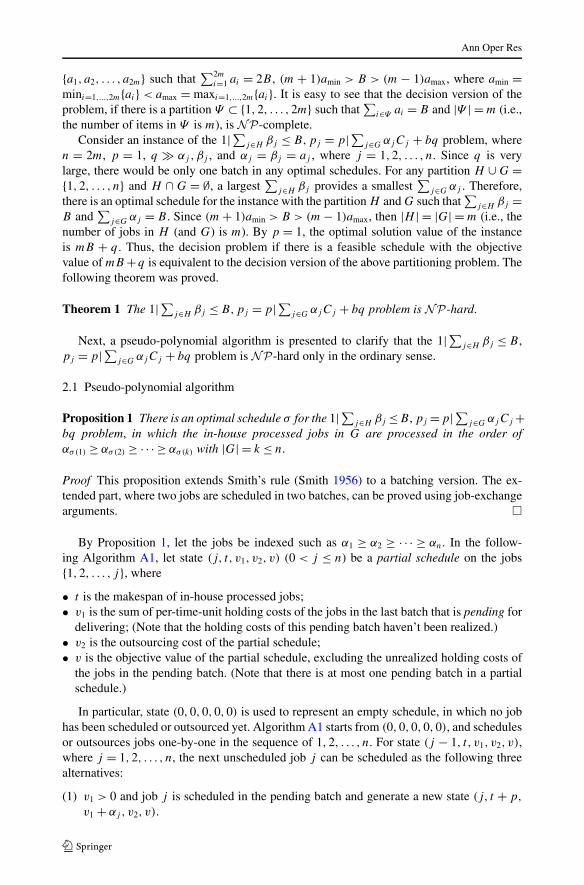
{a1, a2, . . . , a2m} such that∑2m

i=1 ai = 2B , (m + 1)amin > B > (m − 1)amax, where amin =mini=1,...,2m{ai} < amax = maxi=1,...,2m{ai}. It is easy to see that the decision version of theproblem, if there is a partition Ψ ⊂ {1,2, . . . ,2m} such that

∑i∈Ψ ai = B and |Ψ | = m (i.e.,

the number of items in Ψ is m), is NP-complete.Consider an instance of the 1|∑j∈H βj ≤ B,pj = p|∑j∈G αjCj + bq problem, where

n = 2m, p = 1, q αj ,βj , and αj = βj = aj , where j = 1,2, . . . , n. Since q is verylarge, there would be only one batch in any optimal schedules. For any partition H ∪ G ={1,2, . . . , n} and H ∩ G = ∅, a largest

∑j∈H βj provides a smallest

∑j∈G αj . Therefore,

there is an optimal schedule for the instance with the partition H and G such that∑

j∈H βj =B and

∑j∈G αj = B . Since (m + 1)amin > B > (m − 1)amax, then |H | = |G| = m (i.e., the

number of jobs in H (and G) is m). By p = 1, the optimal solution value of the instanceis mB + q . Thus, the decision problem if there is a feasible schedule with the objectivevalue of mB +q is equivalent to the decision version of the above partitioning problem. Thefollowing theorem was proved.

Theorem 1 The 1|∑j∈H βj ≤ B,pj = p|∑j∈G αjCj + bq problem is NP-hard.

Next, a pseudo-polynomial algorithm is presented to clarify that the 1|∑j∈H βj ≤ B ,pj = p|∑j∈G αjCj + bq problem is NP-hard only in the ordinary sense.

2.1 Pseudo-polynomial algorithm

Proposition 1 There is an optimal schedule σ for the 1|∑j∈H βj ≤B , pj =p|∑j∈G αjCj +bq problem, in which the in-house processed jobs in G are processed in the order ofασ(1) ≥ ασ(2) ≥ · · · ≥ ασ(k) with |G| = k ≤ n.

Proof This proposition extends Smith’s rule (Smith 1956) to a batching version. The ex-tended part, where two jobs are scheduled in two batches, can be proved using job-exchangearguments. �

By Proposition 1, let the jobs be indexed such as α1 ≥ α2 ≥ · · · ≥ αn. In the follow-ing Algorithm A1, let state (j, t, v1, v2, v) (0 < j ≤ n) be a partial schedule on the jobs{1,2, . . . , j}, where

• t is the makespan of in-house processed jobs;• v1 is the sum of per-time-unit holding costs of the jobs in the last batch that is pending for

delivering; (Note that the holding costs of this pending batch haven’t been realized.)• v2 is the outsourcing cost of the partial schedule;• v is the objective value of the partial schedule, excluding the unrealized holding costs of

the jobs in the pending batch. (Note that there is at most one pending batch in a partialschedule.)

In particular, state (0,0,0,0,0) is used to represent an empty schedule, in which no jobhas been scheduled or outsourced yet. Algorithm A1 starts from (0,0,0,0,0), and schedulesor outsources jobs one-by-one in the sequence of 1,2, . . . , n. For state (j − 1, t, v1, v2, v),where j = 1,2, . . . , n, the next unscheduled job j can be scheduled as the following threealternatives:

(1) v1 > 0 and job j is scheduled in the pending batch and generate a new state (j, t + p,

v1 + αj , v2, v).

Ann Oper Res

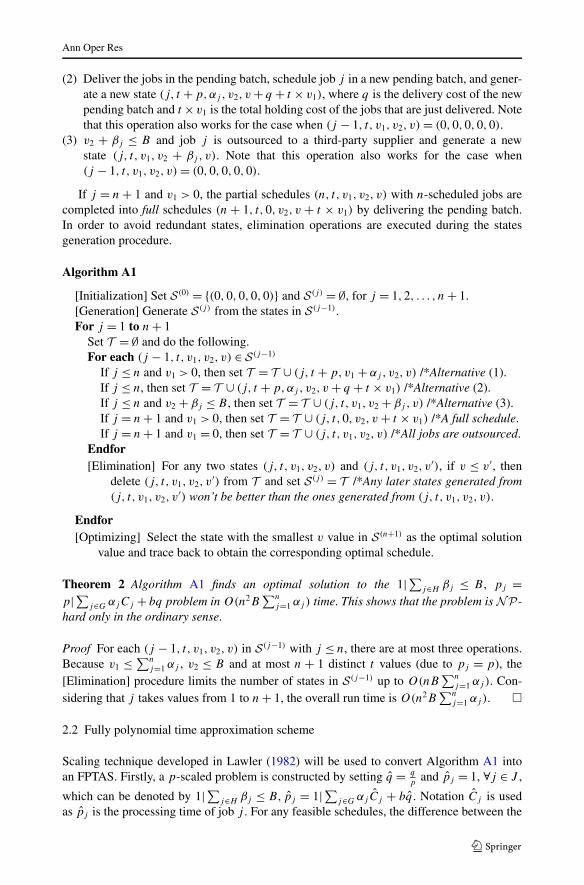
(2) Deliver the jobs in the pending batch, schedule job j in a new pending batch, and gener-ate a new state (j, t + p,αj , v2, v + q + t × v1), where q is the delivery cost of the newpending batch and t ×v1 is the total holding cost of the jobs that are just delivered. Notethat this operation also works for the case when (j − 1, t, v1, v2, v) = (0,0,0,0,0).

(3) v2 + βj ≤ B and job j is outsourced to a third-party supplier and generate a newstate (j, t, v1, v2 + βj , v). Note that this operation also works for the case when(j − 1, t, v1, v2, v) = (0,0,0,0,0).

If j = n + 1 and v1 > 0, the partial schedules (n, t, v1, v2, v) with n-scheduled jobs arecompleted into full schedules (n + 1, t,0, v2, v + t × v1) by delivering the pending batch.In order to avoid redundant states, elimination operations are executed during the statesgeneration procedure.

Algorithm A1

[Initialization] Set S(0) = {(0,0,0,0,0)} and S(j) = ∅, for j = 1,2, . . . , n + 1.[Generation] Generate S(j) from the states in S(j−1).For j = 1 to n + 1

Set T = ∅ and do the following.For each (j − 1, t, v1, v2, v) ∈ S(j−1)

If j ≤ n and v1 > 0, then set T = T ∪ (j, t + p,v1 + αj , v2, v) /*Alternative (1).If j ≤ n, then set T = T ∪ (j, t + p,αj , v2, v + q + t × v1) /*Alternative (2).If j ≤ n and v2 + βj ≤ B , then set T = T ∪ (j, t, v1, v2 + βj , v) /*Alternative (3).If j = n + 1 and v1 > 0, then set T = T ∪ (j, t,0, v2, v + t × v1) /*A full schedule.If j = n + 1 and v1 = 0, then set T = T ∪ (j, t, v1, v2, v) /*All jobs are outsourced.

Endfor[Elimination] For any two states (j, t, v1, v2, v) and (j, t, v1, v2, v

′), if v ≤ v′, thendelete (j, t, v1, v2, v

′) from T and set S(j) = T /*Any later states generated from(j, t, v1, v2, v

′) won’t be better than the ones generated from (j, t, v1, v2, v).

Endfor[Optimizing] Select the state with the smallest v value in S(n+1) as the optimal solution

value and trace back to obtain the corresponding optimal schedule.

Theorem 2 Algorithm A1 finds an optimal solution to the 1|∑j∈H βj ≤ B , pj =p|∑j∈G αjCj + bq problem in O(n2B

∑n

j=1 αj ) time. This shows that the problem is NP-hard only in the ordinary sense.

Proof For each (j − 1, t, v1, v2, v) in S(j−1) with j ≤ n, there are at most three operations.Because v1 ≤ ∑n

j=1 αj , v2 ≤ B and at most n + 1 distinct t values (due to pj = p), the[Elimination] procedure limits the number of states in S(j−1) up to O(nB

∑n

j=1 αj ). Con-sidering that j takes values from 1 to n + 1, the overall run time is O(n2B

∑n

j=1 αj ). �

2.2 Fully polynomial time approximation scheme

Scaling technique developed in Lawler (1982) will be used to convert Algorithm A1 intoan FPTAS. Firstly, a p-scaled problem is constructed by setting q = q

pand pj = 1, ∀j ∈ J ,

which can be denoted by 1|∑j∈H βj ≤ B, pj = 1|∑j∈G αj Cj + bq . Notation Cj is usedas pj is the processing time of job j . For any feasible schedules, the difference between the

Ann Oper Res

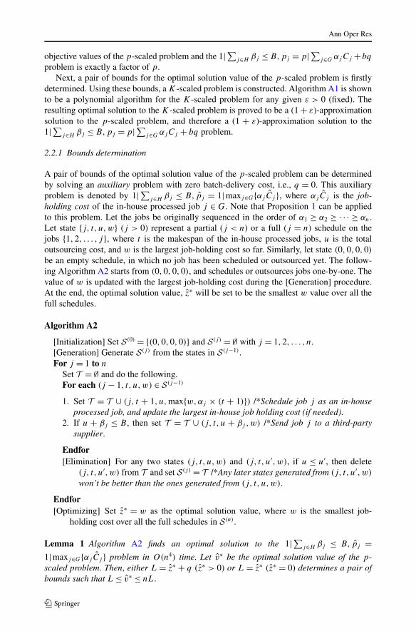
objective values of the p-scaled problem and the 1|∑j∈H βj ≤ B,pj = p|∑j∈G αjCj +bq

problem is exactly a factor of p.Next, a pair of bounds for the optimal solution value of the p-scaled problem is firstly

determined. Using these bounds, a K-scaled problem is constructed. Algorithm A1 is shownto be a polynomial algorithm for the K-scaled problem for any given ε > 0 (fixed). Theresulting optimal solution to the K-scaled problem is proved to be a (1 + ε)-approximationsolution to the p-scaled problem, and therefore a (1 + ε)-approximation solution to the1|∑j∈H βj ≤ B,pj = p|∑j∈G αjCj + bq problem.

2.2.1 Bounds determination

A pair of bounds of the optimal solution value of the p-scaled problem can be determinedby solving an auxiliary problem with zero batch-delivery cost, i.e., q = 0. This auxiliaryproblem is denoted by 1|∑j∈H βj ≤ B, pj = 1|maxj∈G{αj Cj }, where αj Cj is the job-holding cost of the in-house processed job j ∈ G. Note that Proposition 1 can be appliedto this problem. Let the jobs be originally sequenced in the order of α1 ≥ α2 ≥ · · · ≥ αn.Let state {j, t, u,w} (j > 0) represent a partial (j < n) or a full (j = n) schedule on thejobs {1,2, . . . , j}, where t is the makespan of the in-house processed jobs, u is the totaloutsourcing cost, and w is the largest job-holding cost so far. Similarly, let state (0,0,0,0)

be an empty schedule, in which no job has been scheduled or outsourced yet. The follow-ing Algorithm A2 starts from (0,0,0,0), and schedules or outsources jobs one-by-one. Thevalue of w is updated with the largest job-holding cost during the [Generation] procedure.At the end, the optimal solution value, z∗ will be set to be the smallest w value over all thefull schedules.

Algorithm A2

[Initialization] Set S(0) = {(0,0,0,0)} and S(j) = ∅ with j = 1,2, . . . , n.[Generation] Generate S(j) from the states in S(j−1).For j = 1 to n

Set T = ∅ and do the following.For each (j − 1, t, u,w) ∈ S(j−1)

1. Set T = T ∪ (j, t + 1, u,max{w,αj × (t + 1)}) /*Schedule job j as an in-houseprocessed job, and update the largest in-house job holding cost (if needed).

2. If u + βj ≤ B , then set T = T ∪ (j, t, u + βj ,w) /*Send job j to a third-partysupplier.

Endfor[Elimination] For any two states (j, t, u,w) and (j, t, u′,w), if u ≤ u′, then delete

(j, t, u′,w) from T and set S(j) = T /*Any later states generated from (j, t, u′,w)

won’t be better than the ones generated from (j, t, u,w).

Endfor[Optimizing] Set z∗ = w as the optimal solution value, where w is the smallest job-

holding cost over all the full schedules in S(n).

Lemma 1 Algorithm A2 finds an optimal solution to the 1|∑j∈H βj ≤ B, pj =1|maxj∈G{αj Cj } problem in O(n4) time. Let v∗ be the optimal solution value of the p-scaled problem. Then, either L = z∗ + q (z∗ > 0) or L = z∗ (z∗ = 0) determines a pair ofbounds such that L ≤ v∗ ≤ nL.

Ann Oper Res

Proof Because there are at most n distinct t values and n2 distinct w values, after the[Elimination] procedure the number of states in S(j−1) is at most n3. For each (j − 1,

t, u,w) ∈ S(j−1), there are at most two operations. Considering n iterations for j , the overallrun time is O(n4).

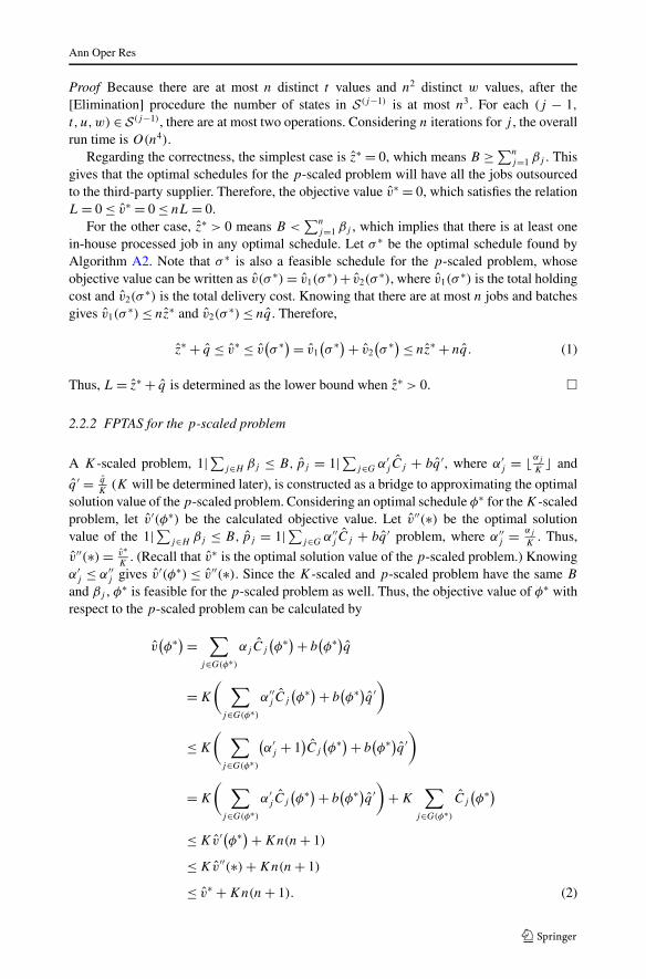
Regarding the correctness, the simplest case is z∗ = 0, which means B ≥ ∑n

j=1 βj . Thisgives that the optimal schedules for the p-scaled problem will have all the jobs outsourcedto the third-party supplier. Therefore, the objective value v∗ = 0, which satisfies the relationL = 0 ≤ v∗ = 0 ≤ nL = 0.

For the other case, z∗ > 0 means B <∑n

j=1 βj , which implies that there is at least onein-house processed job in any optimal schedule. Let σ ∗ be the optimal schedule found byAlgorithm A2. Note that σ ∗ is also a feasible schedule for the p-scaled problem, whoseobjective value can be written as v(σ ∗) = v1(σ

∗)+ v2(σ∗), where v1(σ

∗) is the total holdingcost and v2(σ

∗) is the total delivery cost. Knowing that there are at most n jobs and batchesgives v1(σ

∗) ≤ nz∗ and v2(σ∗) ≤ nq . Therefore,

z∗ + q ≤ v∗ ≤ v(σ ∗) = v1

(σ ∗) + v2

(σ ∗) ≤ nz∗ + nq. (1)

Thus, L = z∗ + q is determined as the lower bound when z∗ > 0. �

2.2.2 FPTAS for the p-scaled problem

A K-scaled problem, 1|∑j∈H βj ≤ B, pj = 1|∑j∈G α′j Cj + bq ′, where α′

j = � αj

K� and

q ′ = q

K(K will be determined later), is constructed as a bridge to approximating the optimal

solution value of the p-scaled problem. Considering an optimal schedule φ∗ for the K-scaledproblem, let v′(φ∗) be the calculated objective value. Let v′′(∗) be the optimal solutionvalue of the 1|∑j∈H βj ≤ B, pj = 1|∑j∈G α′′

j Cj + bq ′ problem, where α′′j = αj

K. Thus,

v′′(∗) = v∗K

. (Recall that v∗ is the optimal solution value of the p-scaled problem.) Knowingα′

j ≤ α′′j gives v′(φ∗) ≤ v′′(∗). Since the K-scaled and p-scaled problem have the same B

and βj , φ∗ is feasible for the p-scaled problem as well. Thus, the objective value of φ∗ withrespect to the p-scaled problem can be calculated by

v(φ∗) =

∑

j∈G(φ∗)

αj Cj

(φ∗) + b

(φ∗)q

= K

( ∑

j∈G(φ∗)

α′′j Cj

(φ∗) + b

(φ∗)q ′

)

≤ K

( ∑

j∈G(φ∗)

(α′

j + 1)Cj

(φ∗) + b

(φ∗)q ′

)

= K

( ∑

j∈G(φ∗)

α′j Cj

(φ∗) + b

(φ∗)q ′

)

+ K∑

j∈G(φ∗)

Cj

(φ∗)

≤ Kv′(φ∗) + Kn(n + 1)

≤ Kv′′(∗) + Kn(n + 1)

≤ v∗ + Kn(n + 1). (2)

Ann Oper Res

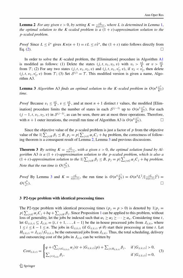
Lemma 2 For any given ε > 0, by setting K = εLn(n+1)

, where L is determined in Lemma 1,the optimal solution to the K-scaled problem is a (1 + ε)-approximation solution to thep-scaled problem.

Proof Since L ≤ v∗ gives Kn(n + 1) = εL ≤ εv∗, the (1 + ε) ratio follows directly fromEq. (2). �

In order to solve the K-scaled problem, the [Elimination] procedure in Algorithm A1is modified as follows: (1) Delete the states (j, t, v1, v2, v) with v1 > nL

Kor v > nL

K

from T ; (2) For any two states (j, t, v1, v2, v) and (j, t, v1, v′2, v), if v2 < v′

2, then delete(j, t, v1, v

′2, v) from T ; (3) Set S(j) = T . This modified version is given a name, Algo-

rithm A3.

Lemma 3 Algorithm A3 finds an optimal solution to the K-scaled problem in O(n4 L2

K2 )

time.

Proof Because v1 ≤ nLK

, v ≤ nLK

, and at most n + 1 distinct t values, the modified [Elim-

ination] procedure limits the number of states in each S(j−1) up to O(n3 L2

K2 ). For each(j − 1, t, v1, v2, v) in S(j−1), as can be seen, there are at most three operations. Therefore,with n + 1 outer iterations, the overall run time of Algorithm A3 is O(n4 L2

K2 ). �

Since the objective value of the p-scaled problem is just a factor of p from the objectivevalue of the 1|∑j∈H βj ≤ B,pj = p|∑j∈G αjCj + bq problem, the correctness of follow-ing theorem is a consequent result of Lemma 2, Lemma 3 and previous discussions.

Theorem 3 By setting K = εLn(n+1)

, with a given ε > 0, the optimal solution found by Al-gorithm A3 is a (1 + ε)-approximation solution to the p-scaled problem, which is also a(1 + ε)-approximation solution to the 1|∑j∈H βj ≤ B,pj = p|∑j∈G αjCj + bq problem.

Note that the run time is O(n8

ε2 ).

Proof By Lemma 3 and K = εLn(n+1)

, the run time is O(n4 L2

K2 ) = O(n4L2/[ εLn(n+1)

]2) =O(n8

ε2 ). �

3 P2-type problem with identical processing times

The P2-type problem with identical processing times (pj = p > 0) is denoted by 1|pj =p|∑j∈G αjCj +bq +∑

j∈H βj . Since Proposition 1 can be applied to this problem, withoutloss of generality, let the jobs be indexed such that α1 ≥ α2 ≥ · · · ≥ αn. Considering time t ,let G(i,k,t) ⊆ J(i,k) = {i, i + 1, . . . , k − 1} be the in-house processed jobs from J(i,k), where1 ≤ i ≤ k − 1 ≤ n. The jobs in G(i,k,t) (if G(i,k,t) �= ∅) start their processing at time t . LetH(i,k,t) = J(i,k)\G(i,k,t) be the outsourced jobs from J(i,k). Thus, the total scheduling, deliveryand outsourcing cost of the jobs in J(i,k) can be written by

Cost(i,k,t) =⎧⎨

⎩

q + (∑

j∈G(i,k,t)αj )(t + |G(i,k,t)|p) + ∑

j∈H(i,k,t)βj , if |G(i,k,t)| > 0,

∑j∈J(i,k)

βj , if |G(i,k,t)| = 0,(3)

Ann Oper Res

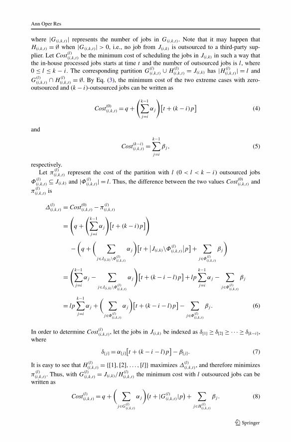
where |G(i,k,t)| represents the number of jobs in G(i,k,t). Note that it may happen thatH(i,k,t) = ∅ when |G(i,k,t)| > 0, i.e., no job from J(i,k) is outsourced to a third-party sup-plier. Let Cost(l)(i,k,t) be the minimum cost of scheduling the jobs in J(i,k) in such a way thatthe in-house processed jobs starts at time t and the number of outsourced jobs is l, where0 ≤ l ≤ k − i. The corresponding partition G

(l)

(i,k,t) ∪ H(l)

(i,k,t) = J(i,k) has |H(l)

(i,k,t)| = l and

G(l)

(i,k,t) ∩ H(l)

(i,k,t) = ∅. By Eq. (3), the minimum cost of the two extreme cases with zero-outsourced and (k − i)-outsourced jobs can be written as

Cost(0)

(i,k,t) = q +(

k−1∑

j=i

αj

)[t + (k − i)p

](4)

and

Cost(k−i)

(i,k,t) =k−1∑

j=i

βj , (5)

respectively.Let π

(l)

(i,k,t) represent the cost of the partition with l (0 < l < k − i) outsourced jobs

Φ(l)

(i,k,t) ⊆ J(i,k) and |Φ(l)

(i,k,t)| = l. Thus, the difference between the two values Cost(0)

(i,k,t) and

π(l)

(i,k,t) is

Δ(l)

(i,k,t) = Cost(0)

(i,k,t) − π(l)

(i,k,t)

=(

q +(

k−1∑

j=i

αj

)[t + (k − i)p

])

−(

q +( ∑

j∈J(i,k)\Φ(l)(i,k,t)

αj

)[t + ∣

∣J(i,k)\Φ(l)

(i,k,t)

∣∣p

] +∑

j∈Φ(l)(i,k,t)

βj

)

=(

k−1∑

j=i

αj −∑

j∈J(i,k)\Φ(l)(i,k,t)

αj

)[t + (k − i − l)p

] + lp

k−1∑

j=i

αj −∑

j∈Φ(l)(i,k,t)

βj

= lp

k−1∑

j=i

αj +( ∑

j∈Φ(l)(i,k,t)

αj

)[t + (k − i − l)p

] −∑

j∈Φ(l)(i,k,t)

βj . (6)

In order to determine Cost(l)(i,k,t), let the jobs in J(i,k) be indexed as δ[1] ≥ δ[2] ≥ · · · ≥ δ[k−i],where

δ[j ] = α[j ][t + (k − i − l)p

] − β[j ]. (7)

It is easy to see that H(l)

(i,k,t) = {[1], [2], . . . , [l]} maximizes Δ(l)

(i,k,t), and therefore minimizes

π(l)

(i,k,t). Thus, with G(l)

(i,k,t) = J(i,k)/H(l)

(i,k,t) the minimum cost with l outsourced jobs can bewritten as

Cost(l)(i,k,t) = q +( ∑

j∈G(l)(i,k,t)

αj

)(t + |G(l)

(i,k,t)|p) +

∑

j∈H(l)(i,k,t)

βj . (8)

Ann Oper Res

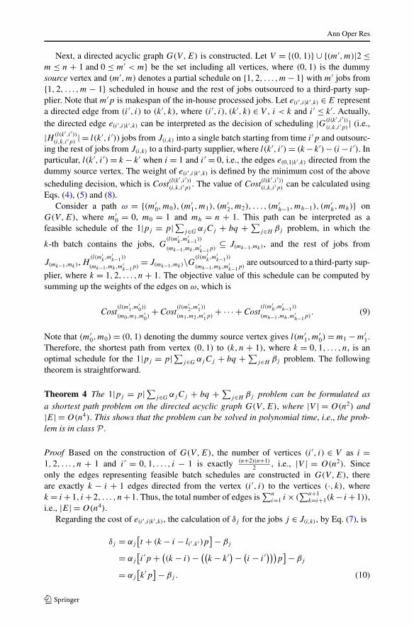
Next, a directed acyclic graph G(V,E) is constructed. Let V = {(0,1)} ∪ {(m′,m)|2 ≤m ≤ n + 1 and 0 ≤ m′ < m} be the set including all vertices, where (0,1) is the dummysource vertex and (m′,m) denotes a partial schedule on {1,2, . . . ,m − 1} with m′ jobs from{1,2, . . . ,m − 1} scheduled in house and the rest of jobs outsourced to a third-party sup-plier. Note that m′p is makespan of the in-house processed jobs. Let e(i′,i|k′,k) ∈ E representa directed edge from (i ′, i) to (k′, k), where (i ′, i), (k′, k) ∈ V , i < k and i ′ ≤ k′. Actually,the directed edge e(i′,i|k′,k) can be interpreted as the decision of scheduling |G(l(k′,i′))

(i,k,i′p)| (i.e.,

|H(l(k′,i′))(i,k,i′p)

| = l(k′, i ′)) jobs from J(i,k) into a single batch starting from time i ′p and outsourc-ing the rest of jobs from J(i,k) to a third-party supplier, where l(k′, i ′) = (k −k′)− (i − i ′). Inparticular, l(k′, i ′) = k − k′ when i = 1 and i ′ = 0, i.e., the edges e(0,1|k′,k) directed from thedummy source vertex. The weight of e(i′,i|k′,k) is defined by the minimum cost of the above

scheduling decision, which is Cost(l(k′,i′))

(i,k,i′p). The value of Cost(l(k

′,i′))(i,k,i′p)

can be calculated usingEqs. (4), (5) and (8).

Consider a path ω = {(m′0,m0), (m

′1,m1), (m

′2,m2), . . . , (m

′h−1,mh−1), (m

′h,mh)} on

G(V,E), where m′0 = 0, m0 = 1 and mh = n + 1. This path can be interpreted as a

feasible schedule of the 1|pj = p|∑j∈G αjCj + bq + ∑j∈H βj problem, in which the

k-th batch contains the jobs, G(l(m′

k,m′

k−1))

(mk−1,mk,m′k−1p)

⊆ J(mk−1,mk), and the rest of jobs from

J(mk−1,mk), H(l(m′

k,m′

k−1))

(mk−1,mk,m′k−1p)

= J(mk−1,mk)\G(l(m′k,m′

k−1))

(mk−1,mk,m′k−1p)

are outsourced to a third-party sup-

plier, where k = 1,2, . . . , n + 1. The objective value of this schedule can be computed bysumming up the weights of the edges on ω, which is

Cost(l(m′

1,m′0))

(m0,m1,m′0)

+ Cost(l(m′

2,m′1))

(m1,m2,m′1p)

+ · · · + Cost(l(m′

h,m′

h−1))

(mh−1,mh,m′h−1p)

. (9)

Note that (m′0,m0) = (0,1) denoting the dummy source vertex gives l(m′

1,m′0) = m1 − m′

1.Therefore, the shortest path from vertex (0,1) to (k, n + 1), where k = 0,1, . . . , n, is anoptimal schedule for the 1|pj = p|∑j∈G αjCj + bq + ∑

j∈H βj problem. The followingtheorem is straightforward.

Theorem 4 The 1|pj = p|∑j∈G αjCj + bq + ∑j∈H βj problem can be formulated as

a shortest path problem on the directed acyclic graph G(V,E), where |V | = O(n2) and|E| = O(n4). This shows that the problem can be solved in polynomial time, i.e., the prob-lem is in class P .

Proof Based on the construction of G(V,E), the number of vertices (i ′, i) ∈ V as i =1,2, . . . , n + 1 and i ′ = 0,1, . . . , i − 1 is exactly (n+2)(n+1)

2 , i.e., |V | = O(n2). Sinceonly the edges representing feasible batch schedules are constructed in G(V,E), thereare exactly k − i + 1 edges directed from the vertex (i ′, i) to the vertices (·, k), wherek = i +1, i +2, . . . , n+1. Thus, the total number of edges is

∑n

i=1 i × (∑n+1

k=i+1(k − i +1)),i.e., |E| = O(n4).

Regarding the cost of e(i′,i|k′,k), the calculation of δj for the jobs j ∈ J(i,k), by Eq. (7), is

δj = αj

[t + (k − i − li′,k′)p

] − βj

= αj

[i ′p + (

(k − i) − ((k − k′) − (

i − i ′)))p] − βj

= αj

[k′p

] − βj . (10)

Ann Oper Res

This implies that for each job j , there are n+1 possible δj values due to the n+1 selectionsof k′, i.e., k′ = 0,1, . . . , n. For each given k′, a sequence of the jobs in J(i,k) with the non-increasing order of δj can be easily determined by Eq. (10). Thus, by pre-determining then + 1 sequences for the n jobs, which can be done in O(n3 logn) time, the costs and theset of ordered jobs for the edges in E can be finally established. This demonstrates thatG(V,E) can be constructed in polynomial time, and therefore the 1|pj = p|∑j∈G αjCj +bq + ∑

j∈H βj problem is in class P . �

Next, the above shortest-path-problem formulation is modified to deal with the specialcase of the Modified-P2 problem with identical processing times, denoted by 1|pj = p,b ≤R|∑j∈G αjCj +∑

j∈H βj . Since the holding costs, outsourcing costs and batching decisionsconsidered in this special case are also considered by the 1|pj = p|∑j∈G αjCj + bq +∑

j∈H βj problem, the topology structure of G(V,E) can also used to formulate this specialcase. Because delivery costs are not included in the special case, q is removed from Eq. (8).With these edge costs, the modified G(V,E) is denoted by G(V ,E), which has the samenodes, edges and scheduling interpretations as G(V,E). Since the number of deliveries isupper bounded, the special case is to find a shortest path on G(V ,E) with R edges at most.This modified shortest path problem is a special case of the delay constrained least cost path(DCLC) problem (Cheng and Ansari 2003) with one-unit time delay on each edge. For thegeneral DCLC problem, Garey and Johnson (1979) proved the NP-hardness and Hassin(1992) presented a dynamic programming algorithm running in O(|E|T ) time, where T

is the upper bound of time delays. Since G(V ,E) has |E| = O(n4) and T = R ≤ n inO(|E|T ), the following theorem is proved.

Theorem 5 The 1|pj = p,b ≤ R|∑j∈G αjCj + ∑j∈H βj problem can be formulated as

a special case of DCLC problem on G(V ,E) with one-unit time delay on each edge,where |V | = O(n2) and |E| = O(n4). Using the dynamic programming algorithm in Has-sin (1992), this formulation can be solved in O(|E|R) = O(n5) time. This shows that thespecial case of Modified-P2 problem is in class P .

4 Conclusions

In this paper, the problem of minimizing the total holding and delivery costs with outsourc-ing was studied. Since the general problem is strongly NP-hard, two special cases withidentical processing times were investigated. The P1-type problem with limited outsourcingbudgets was shown to be NP-hard only in the ordinary sense by the presented NP-hardnessproof and pseudo-polynomial algorithm. The pseudo-polynomial algorithm was further con-verted into an FPTAS. By allowing unlimited outsourcing budgets, the P2-type problem wasformulated and solved as a shortest path problem. This showed that the P2-type problem isin class P .

Regarding the Modified-P2 problem, where the number of deliveries is upper-bounded,its special case with identical processing times was shown to be equivalent to the delayconstrained least cost path problem, where the time delay on each edge is one. Thus, thisspecial case can be solved in polynomial time and therefor in class P .

For future research, the Modified-P2 problem with arbitrary processing times is open tocomplexity studies and solution approaches. Knowing that the P1 and P2-type problems witharbitrary processing times are strongly NP-hard, heuristics or approximations are deserveresearchers’ efforts.

Ann Oper Res

References

Agnetis, A., Hall, N. G., & Pacciarelli, D. (2006). Supply chain scheduling: sequence coordination. DiscreteApplied Mathematics, 154(15), 2044–2063.

Chen, Z.-L. (2010). Integrated production and outbound distribution scheduling: review and extensions. Op-erations Research, 58(1), 130–148.

Chen, Z.-L., & Hall, N. G. (2007). Supply chain scheduling: conflict and cooperation in assembly systems.Operations Research, 55, 1072–1089.

Chen, Z.-L., & Vairaktarakis, G. L. (2005). Integrated scheduling of production and distribution operations.Management Science, 51, 614–628.

Cheng, G., & Ansari, N. (2003). A new heuristics for finding the delay constrained least cost path. IEEEGlobal Telecommunications Conference (GLOBECOM’03), 2003(7), 3711–3715.

Engels, D. W., Karger, D. R., Kolliopoulos, S. G., Sengupta, S., Uma, R. N., & Wein, J. (2003). Techniquesfor scheduling with rejection. Journal of Algorithms, 49(1), 175–191.

Garey, M. R., & Johnson, D. S. (1979). Computers and intractability: a guide to the theory of NP-completeness. New York: Freeman. 1979.

Graham, R. L., Lawler, E. L., Lenstra, J. K., & Rinnooy Kan, A. H. G. (1979). Optimization and approxima-tion in deterministic sequencing and scheduling: a survey. Annals of Discrete Mathematics, 4, 287–326.

Hall, N. G., & Potts, C. N. (2003). Supply chain scheduling, batching and delivery. Operations Research,51(4), 566–584.

Hassin, R. (1992). Approximation schemes for the restricted shortest path problem. Mathematics of Opera-tions Research, 17(1), 36–42.

Lawler, E. L. (1982). A fully polynomial time approximation scheme for the total tardiness problem. Opera-tions Research Letters, 1(6), 207–208.

McKenna Long & Aldridge LLP (2004). Recent budget provision limits offshoring of jobs under out-sourced federal contracts: legislation introduced. In Several states related to state procurements. www.mckennalong.com.

Qi, X. T. (2008). Coordinated logistics scheduling for in-house production and outsourcing. IEEE Transac-tions on Automation Science and Engineering, 5(1), 188–192.

Selvarajah, E., & Steiner, G. (2009). Approximation algorithms for the supplier’s supply chain schedulingproblem to minimize delivery and inventory holding costs. Operations Research, 57(2), 426–438.

Selvarajah, E., Steiner, G., & Zhang, R. (2011). Single machine batch scheduling with release times anddelivery costs. Journal of Scheduling. Online FirstTM. doi:10.1007/s10951-011-0255-8.

Shabtay, D., Gaspar, N., & Kaspi, M. (2013). A survey on offline scheduling with rejection. Journal ofScheduling, 16, 2–282.

Shabtay, D., & Steiner, G. (2007). A survey of scheduling with controllable processing times. Discrete Ap-plied Mathematics, 155(13), 1643–1666.

Smith, W. E. (1956). Various optimizers for single-stage production. Naval Research Logistics Quarterly, 3,59–66.

Steiner, G., & Zhang, R. (2011). Revised delivery-time quotation in scheduling with tardiness penalties.Operations Research, 59(6), 1504–1511.

Thomas, D. J., & Griffin, P. M. (1996). Coordinated supply chain management. European Journal of Opera-tional Research, 94, 1–15.

Wang, X. L., & Cheng, T. C. E. (2009). Production scheduling with supply and delivery considerations tominimize the makespan. European Journal of Operational Research, 194(3), 743–752.

Zhang, L. Q., Lu, L. F., & Yuan, J. J. (2010). Single-machine scheduling under the job rejection constraint.Theoretical Computer Science, 411(16–18), 1877–1882.