Surface Flow from Visual Cues - hal.inria.fr · Flot de surface à partir d’indices visuels ... Dans cette optique, ... and Kanade (1981) have been proposed

HAL Id: inria-00593206https://hal.inria.fr/inria-00593206v2

Submitted on 17 May 2011

HAL is a multi-disciplinary open accessarchive for the deposit and dissemination of sci-entific research documents, whether they are pub-lished or not. The documents may come fromteaching and research institutions in France orabroad, or from public or private research centers.

L’archive ouverte pluridisciplinaire HAL, estdestinée au dépôt et à la diffusion de documentsscientifiques de niveau recherche, publiés ou non,émanant des établissements d’enseignement et derecherche français ou étrangers, des laboratoirespublics ou privés.

Surface Flow from Visual CuesBenjamin Petit, Antoine Letouzey, Edmond Boyer

To cite this version:Benjamin Petit, Antoine Letouzey, Edmond Boyer. Surface Flow from Visual Cues. [Research Report]RR-7619, INRIA. 2011, pp.18. <inria-00593206v2>

https://hal.inria.fr/inria-00593206v2

https://hal.archives-ouvertes.fr

appor t de r ech er ch e

ISS

N02

49-6

399

ISR

NIN

RIA

/RR

--76

19--

FR+E

NG

Domaine 4

INSTITUT NATIONAL DE RECHERCHE EN INFORMATIQUE ET EN AUTOMATIQUE

Surface Flow from Visual Cues

Benjamin Petit — Antoine Letouzey — Edmond Boyer

N° 7619

May 2011

Centre de recherche INRIA Grenoble – Rhône-Alpes655, avenue de l’Europe, 38334 Montbonnot Saint Ismier

Téléphone : +33 4 76 61 52 00 — Télécopie +33 4 76 61 52 52

Surface Flow from Visual Cues

Benjamin Petit, Antoine Letouzey, Edmond Boyer

Domaine : Perception, cognition, interactionÉquipe-Projet Morpheo

Rapport de recherche n° 7619 — May 2011 — 18 pages

Abstract: In this paper we study the estimation of dense, instantaneous 3D motionfields over non-rigidly moving surface observed by multi-camera systems. The moti-vation arises from multi-camera applications that require motion information for arbi-trary subjects, in order to perform tasks such as surface tracking or segmentation. Tothis aim, we present a novel framework that allows to efficiently compute dense 3D dis-placement fields using low level visual cues and geometric constraints. The main con-tribution is a unified framework that combines flow constraints for small displacementswith temporal feature constraints for large displacements and fuses them over the sur-face using local rigidity constraints. The resulting linear optimization problem allowsfor variational solutions and fast implementations. Experiments conducted on syntheticand real data demonstrate the respective interests of flow and feature constraints as wellas their efficiency to provide robust surface motion cues when combined.

Key-words: Surface, flow, 3D motion

Flot de surface à partir d’indices visuelsRésumé : Dans ce papier nous nous intéressons à l’estimation des champs de dé-placement denses d’une surface non rigide, en mouvement, capturée par un systèmemulti-caméra. La motivation vient des applications multi-caméra qui nécessitent uneinformation de mouvement pour accomplir des tâches telles que le suivi de surface ou lasegmentation. Dans cette optique, nous présentons une approche nouvelle, qui permetde calculer efficacement un champ de déplacement 3D, en utilisant des informations vi-suelles de bas niveau et des contraintes géométriques. La contribution principale est laproposition d’un cadre unifié qui combine des contraintes de flot pour de petits déplace-ments et des correspondances temporelles éparses pour les déplacements importants.Ces deux types d’informations sont fusionnés sur la surface en utilisant une contraintede rigidité locale. Le problème se formule comme une optimisation linéaire permettantune implémentation rapide grâce à une approche variationelle. Les expérimentationsmenées sur des données synthétiques et réelles démontrent les intérêts respectifs duflot et des informations éparses, ainsi que leur efficacité conjointe pour calculer lesdéplacements d’une surface de manière robuste.

Mots-clés : Surface, flot, déplacements 3D

Surface Flow from Visual Cues 3

Contents1 Introduction 3

2 Related Work 4

3 Preliminaries and Definitions 5

4 Visual Constraints 64.1 Dense 2D Normal Flow . . . . . . . . . . . . . . . . . . . . . . . . . 74.2 Sparse 2D Features . . . . . . . . . . . . . . . . . . . . . . . . . . . 74.3 Sparse 3D Features . . . . . . . . . . . . . . . . . . . . . . . . . . . 8

5 Regularization 95.1 Deformation Model . . . . . . . . . . . . . . . . . . . . . . . . . . . 95.2 Energy Functional Minimization . . . . . . . . . . . . . . . . . . . . 105.3 Selection of Weights and 2-Pass Refinement . . . . . . . . . . . . . . 10

6 Evaluation 116.1 Quantitative Evaluation on Synthetic Data . . . . . . . . . . . . . . . 126.2 Comparison . . . . . . . . . . . . . . . . . . . . . . . . . . . . . . . 136.3 Experiments on Real Data . . . . . . . . . . . . . . . . . . . . . . . 14

7 Conclusion 14

1 IntroductionRecovering dense motion information is a fundamental intermediate step in the imageprocessing chain upon which higher level applications can be built, such as tracking orsegmentation. For that purpose, pixel observations in the image provide useful motioncues through temporal variations of the intensity function. In the monocular case thesevariations allow to recover a dense 2D motion field in the image: the optical flow. Theestimation of the optical flow has been a subject of interest in the vision community fordecades and numerous methods Barron et al. (1994); Horn and Schunck (1981); Lucasand Kanade (1981) have been proposed. In the multiocular case, the integration overdifferent viewpoints allow to consider 3D motions of points on the observed surfacesand to estimate dense 3D vector fields: the scene flow Neumann and Aloimonos (2002);Vedula et al. (2005). However, in both 2D and 3D cases, the motion information cannotbe determined independently at a point from intensity variations only and additionalconstraints between points must be introduced, smoothness for example. Moreover, asa result of finite difference approximations of derivatives, flow estimations are knownto be limited to small motions. While several approaches have been proposed in 2D tocope with these limitations Xu et al. (2010), less efforts have been devoted to the 3Dcase.

In this paper we study how to incorporate, in an efficient way, various constraintswhen estimating dense motion information over 3D surfaces from temporal variationsof the intensity function in several images. Our primary motivation is to provide robustmotion cues that can be directly used by an application, e.g. interactive applications, orthat can be fed into more advanced tasks such as surface tracking or segmentation, e.g.into rigid parts. The approach is however not limited to a specific scenario and applies

RR n° 7619


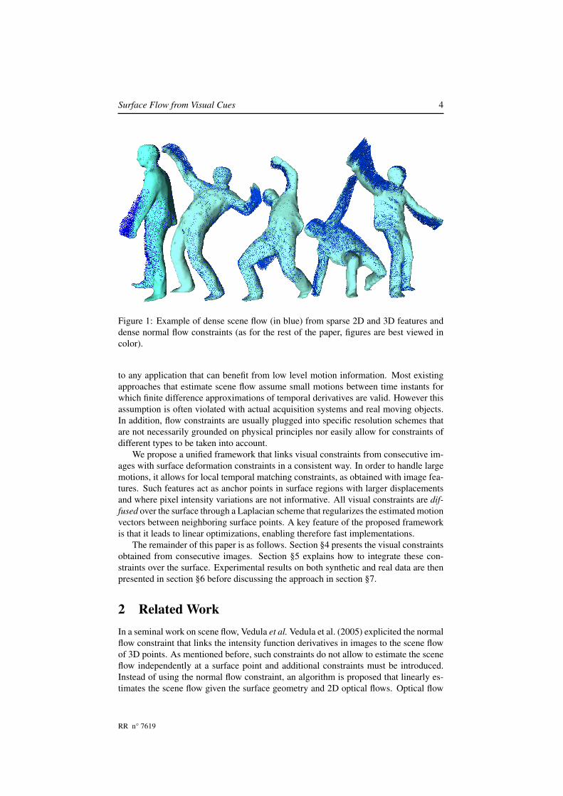
Figure 1: Example of dense scene flow (in blue) from sparse 2D and 3D features anddense normal flow constraints (as for the rest of the paper, figures are best viewed incolor).

to any application that can benefit from low level motion information. Most existingapproaches that estimate scene flow assume small motions between time instants forwhich finite difference approximations of temporal derivatives are valid. However thisassumption is often violated with actual acquisition systems and real moving objects.In addition, flow constraints are usually plugged into specific resolution schemes thatare not necessarily grounded on physical principles nor easily allow for constraints ofdifferent types to be taken into account.

We propose a unified framework that links visual constraints from consecutive im-ages with surface deformation constraints in a consistent way. In order to handle largemotions, it allows for local temporal matching constraints, as obtained with image fea-tures. Such features act as anchor points in surface regions with larger displacementsand where pixel intensity variations are not informative. All visual constraints are dif-fused over the surface through a Laplacian scheme that regularizes the estimated motionvectors between neighboring surface points. A key feature of the proposed frameworkis that it leads to linear optimizations, enabling therefore fast implementations.

The remainder of this paper is as follows. Section §4 presents the visual constraintsobtained from consecutive images. Section §5 explains how to integrate these con-straints over the surface. Experimental results on both synthetic and real data are thenpresented in section §6 before discussing the approach in section §7.

2 Related WorkIn a seminal work on scene flow, Vedula et al. Vedula et al. (2005) explicited the normalflow constraint that links the intensity function derivatives in images to the scene flowof 3D points. As mentioned before, such constraints do not allow to estimate the sceneflow independently at a surface point and additional constraints must be introduced.Instead of using the normal flow constraint, an algorithm is proposed that linearly es-timates the scene flow given the surface geometry and 2D optical flows. Optical flow

RR n° 7619


better constrains the scene flow than the normal flow, however their estimation is basedon smoothness assumptions that seldom hold in the image planes whereas they oftendo on surfaces.

In Neumann and Aloimonos (2002), Neumann and Aloimonos introduced an ele-gant subdivision surface model that allows to integrate normal flow constraints over thesurface with regularization constraints. Nevertheless, this global solution still assumessmall motions and can hardly deal with challenging datasets as used in this paper.

Another strategy is followed by Pons et al. Pons et al. (2005) who presented a vari-ational framework that optimizes a photo-consistency criterion instead of the normalflow constraints. The interest is that both spatial and temporal consistency can be en-forced but at the price of a computationally expensive optimization. In contrast, ourfocus is not on shape optimization but more on providing low level motion informationin an efficient way. Several works Isard and MacCormick (2006); Wedel et al. (2008);Zhang and Kambhamettu (2001) consider the case where the scene structure is de-scribed by stereo disparities and propose combined estimation of spatial disparity andtemporal 3D motion. We consider a different situation where the shape surface is given,e.g. a mesh obtained using a multi-view approach, thus allowing for a regularization ofthe motion field over a domain where smoothness assumptions hold.

It is worth also mentioning recent approaches on temporal surface tracking Cagniartet al. (2010); Naveed et al. (2008); Starck and Hilton (2007b); Varanasi et al. (2008) thatcan also provide velocity fields as a by-product of the matching between consecutiveframes. Our purpose is anyway different since our method does not make any assump-tion on the observed shape and only weak assumptions on the deformation model inthe form of local smoothness assumptions. It provides information at a lower level,instant motion, that can in turn be used as input data by a surface tracking or matchingapproach.

Our contributions with respect to the aforementioned approaches are twofold: (i)Following works on robust optical flow estimation Liu et al. (2008); Xu et al. (2010),we take advantage of robust initial displacement values as provided by image featurestracked over consecutive time instants. Such features allow for large surface motionswhile normal flow constraints better model small motions. (ii) A linear frameworkthat combines visual constraints with surface deformation constraints and allows foriterative resolutions (variational approach) as well as coarse to fine refinement.

3 Preliminaries and DefinitionsOur method deals with the output of any multi-camera system capable of producinga stream of non-rigidly moving surfaces, each independently reconstructed from a setof N calibrated views, using a 3D reconstruction technique such as Franco and Boyer(2008) or Furukawa and Ponce (2006).

The surface at time t is denoted St ⊂ R3 and associated with the set of imagesIt = It

c | c ∈ [1..N ]. A 3D point P on the surface is described by the 3D vector(x, y, z)T ∈ R3. Its projection in the image It

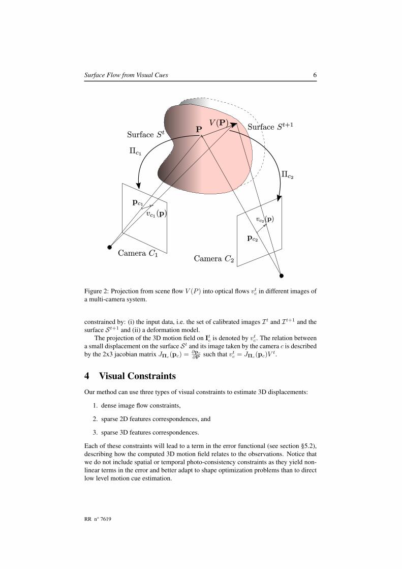
c is the 2D image point pc with coor-dinates (uc, vc)T ∈ R2 computed using the 3x4 projection matrix Πc : R3 7→ R2 ofcamera c (see figure 2). The 2D image region corresponding to the visibility of St inItc is denoted by Ωt

c = ΠcSt.Our method is looking for the 3D motion field of the surface between time t and

t + 1 described by V t : St 7→ R3 with V t(P) = dPdt ∀ P ∈ St. This motion field is

RR n° 7619


Figure 2: Projection from scene flow V (P ) into optical flows vtc in different images of

a multi-camera system.

constrained by: (i) the input data, i.e. the set of calibrated images It and It+1 and thesurface St+1 and (ii) a deformation model.

The projection of the 3D motion field on Itc is denoted by vt

c. The relation betweena small displacement on the surface St and its image taken by the camera c is describedby the 2x3 jacobian matrix JΠc

(pc) = ∂pc

∂P such that vtc = JΠc

(pc)V t.

4 Visual ConstraintsOur method can use three types of visual constraints to estimate 3D displacements:

1. dense image flow constraints,

2. sparse 2D features correspondences, and

3. sparse 3D features correspondences.

Each of these constraints will lead to a term in the error functional (see section §5.2),describing how the computed 3D motion field relates to the observations. Notice thatwe do not include spatial or temporal photo-consistency constraints as they yield non-linear terms in the error and better adapt to shape optimization problems than to directlow level motion cue estimation.

RR n° 7619


4.1 Dense 2D Normal FlowDense information on V t can be classically obtained using the 2D optical flow infor-mation available in the images. Indeed, assuming brightness constancy between pt+1

c

and ptc, projection of the same surface point on two consecutive frames, one can write

the Normal Flow Equation Barron et al. (1994) as:

∇Itc.v

tc +

dItc

dt= 0 ,

or ∇Itc.[JΠc

V t]

+dIt

c

dt= 0 ,

as expressed from 3D surface velocities Vedula et al. (2005);∇Itc is the spatial gradient

of the image intensity and dItc

dt is the temporal gradient of image intensity. We can thendefine an error term measuring the discrepancy between the computed 2D motion fieldvt

c and the normal flow constraints:

Eflow =N∑

c=1

∫Ωt

c

‖∇Itc.[JΠc

V t]

+dIt

c

dt‖2 dpc . (1)

This term is the most common among scene flow methods and well suited for smallimage displacements, but has important limitations: it only constrains the image dis-placements in the direction of the image gradient ∇It

c, or the normal component ofthe optical flow. This is the aperture problem in 2D that extends to 3D as will be dis-cussed in 5. Also, linearization based on the image gradient is typically invalid forlarge displacements.

4.2 Sparse 2D FeaturesIn some situations, e.g. slow motion or high frame rates, motion field recovery canrely on dense normal flow constraints alone. However, in a more general context, ad-ditional constraints must be considered. To this purpose, we propose the use of sparse2D correspondences between the set of images It and It+1 as 2D anchor points toguide the flow estimation. Such features are easily obtained using one of various pop-ular techniques, e.g. SIFT Lowe (2004). Importantly, we opt to match features amongsubsequent frames of the same camera and not between views: First, this eliminatesany need for inter-camera exposure and color calibration. More importantly, the matchand outlier rates between such images are substantially more favorable than for inter-camera matching. This is especially true for the challenging data targeted: general sub-jects with low-to-average textureness, object-centered setups exhibiting wide baselinesby nature. Any remaining outliers can thus be easily eliminated using a conservativematching threshold, as validated in our experiments.

We compute SIFT descriptors for It and It+1, then match features between Itc and

It+1c , with c ∈ [1..N ]. This yields a set of sparse 2D displacements vt

c,s for some 2Dpoints pc,s ∈ Ωt

c, those points form a subset of Ωtc called Ωt

c,s (see figure 3). Thefollowing error term measures the discrepancy between the computed 2D motion field

RR n° 7619


vtc and the sparse 2D displacements vt

c,s:

E2D =N∑

c=1

∑Ωt

c,s

‖vtc − vt

c,s‖2 , or

E2D =N∑

c=1

∑Ωt

c,s

‖JΠcV t − vt

c,s‖2 , (2)

where (2) is the linearization we use. Unlike the normal flow equation, this approxi-mation is still valid for moderate displacements as it doesn’t involve image gradients.

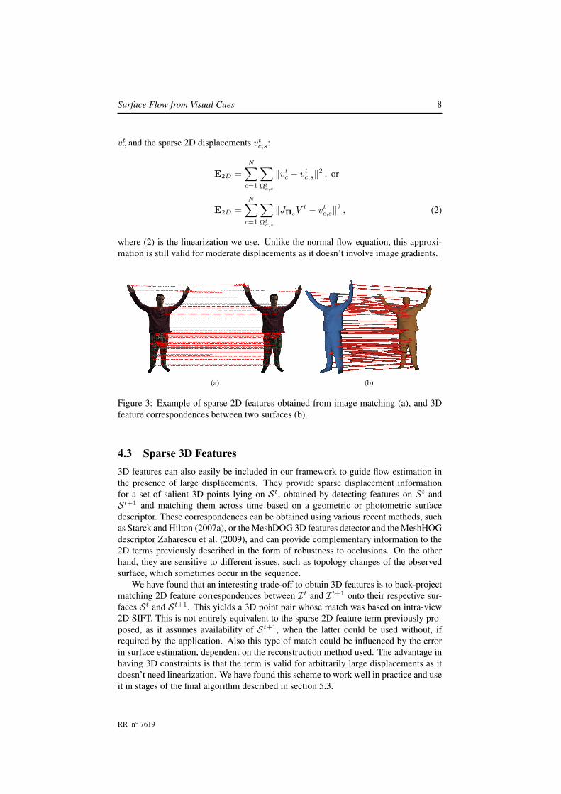
(a) (b)

Figure 3: Example of sparse 2D features obtained from image matching (a), and 3Dfeature correspondences between two surfaces (b).

4.3 Sparse 3D Features3D features can also easily be included in our framework to guide flow estimation inthe presence of large displacements. They provide sparse displacement informationfor a set of salient 3D points lying on St, obtained by detecting features on St andSt+1 and matching them across time based on a geometric or photometric surfacedescriptor. These correspondences can be obtained using various recent methods, suchas Starck and Hilton (2007a), or the MeshDOG 3D features detector and the MeshHOGdescriptor Zaharescu et al. (2009), and can provide complementary information to the2D terms previously described in the form of robustness to occlusions. On the otherhand, they are sensitive to different issues, such as topology changes of the observedsurface, which sometimes occur in the sequence.

We have found that an interesting trade-off to obtain 3D features is to back-projectmatching 2D feature correspondences between It and It+1 onto their respective sur-faces St and St+1. This yields a 3D point pair whose match was based on intra-view2D SIFT. This is not entirely equivalent to the sparse 2D feature term previously pro-posed, as it assumes availability of St+1, when the latter could be used without, ifrequired by the application. Also this type of match could be influenced by the errorin surface estimation, dependent on the reconstruction method used. The advantage inhaving 3D constraints is that the term is valid for arbitrarily large displacements as itdoesn’t need linearization. We have found this scheme to work well in practice and useit in stages of the final algorithm described in section 5.3.

RR n° 7619


Regardless of how they are obtained, let V tm be the displacements of the detected

feature points Pm ∈ St (see figure 3). These points form a discrete subset of St calledSt

m. Being measured directly as a 3D distance, the error between the computed 3D mo-tion field V t and the target 3D displacements V t

m can be written without linearization:

E3D =∑St

m

‖V t − V tm‖2 . (3)

5 RegularizationThe sparse set of 2D and 3D correspondences only constrains the displacement of thesurface for specific 3D points and for their re-projection on the images. To find adense motion field over the surface we need to propagate those constraints through aregularization term.

Furthermore, as mentioned earlier, dense 2D normal flow constraints do not pro-vide enough information to estimate 3D displacements. In fact it can be shown thatthe normal flow equations at different image projections of a 3D point P are linearlydependent, an can only solve 2 of the 3 dofs. Vedula et al. Vedula et al. (2005) men-tioned two regularization strategies to cope with this limitation. The regularization canbe performed in the image planes to estimate optical flows which provide then fullconstraints on the scene flow, or the regularization can be performed on the 3D surface.

Since we are given the 3D surface and that sparse constraints from 2D or 3D fea-tures need to be integrated, a natural choice in our context is to regularize in 3D. Inaddition regularization in the image space suffers from artifacts and incoherences re-sulting from depth discontinuities and occlusions that contradict the smoothness as-sumption whereas such assumption holds on the 3D surface.

5.1 Deformation ModelSmoothness assumptions on 3D displacements fields over a surface constrain the sur-face deformations locally. They thus define a deformation model of the surface, e.g.local rigidity. In 2D, numerous regularization schemes have been proposed for the op-tical flow estimation that fall into 2 main categories: local and global regularizations.They can be extended to 3D. For example, the 2D Lucas and Kanade method, whichuses a local spatial neighborhood, was applied in 3D by Devernay et al. Devernayet al. (2006). However, the associated deformation model of the surface has no realmeaning since deformation constraints only propagate locally, yielding inconsistenciesbetween neighborhoods. On the other hand, the global strategy introduced by Horn andSchunck Horn and Schunck (1981) is well suited to our context. Though less robust tonoise than local methods such as Lucas-Kanade, it allows sparse constraint propaga-tion over the whole surface. In addition the associated surface deformation model hasproved to be efficient in the computer graphics domain Sorkine and Alexa (2007).

The extension of Horn and Schunck deformation model to 3D points is describedby the following error function which enforce a local rigidity of the motion field:

Ed =∫

S

‖∇V ‖2dP . (4)

RR n° 7619


5.2 Energy Functional MinimizationWe find the best displacement that satisfies all the aforementioned constraints by min-imizing the following error functional:

arg minV

[λ2

3DE3D + λ22DE2D + λ2

flowEflow + λ2dEd

],

where the different λ coefficients are parameters that can be set to give more weight toa particular constraint.

This functional can be minimized by solving its associated Euler-Lagrange equa-tion:

NXc=1

»λ2

flow

»∇It

c.ˆJΠcV

t˜+dIt

c

dt

–+ λ2

2DδΩtc,sJΠc

ˆV t − V t

c,s

˜–+λ2

3DδStm

ˆV t − V t

m

˜+ λ2

d∇2V t = 0 ,

(5)

where δ is the Kronecker symbol, denoting that this constraint is only defined for 3Dpoints in St

m or Ωtc,s.

The discretized Euler-Lagrange equation for each 3D points P of the surface hasthe form:

APVP + bP −∆VP = 0 , (6)

where ∆ is the normalized Laplace-Beltrami operator over the surface.The combination of equation (6) for all 3D points P ∈ St creates a simple linear

system of the form: [LA

]V t +

[0b

]= 0 , (7)

where L is the Laplacian matrix as defined in Sorkine and Alexa (2007). This is asparse linear system which can be solved using a sparse solver such as Taucs.

Note that, interestingly, this formulation revisits the Laplacian mesh editing inan as-rigid-as-possible way of the computer graphics community Sorkine and Alexa(2007). While the deformation model is similar, the difference lies in the constraintused: anchor points in Sorkine and Alexa (2007) and visual constraints in our approach.In both cases, it is known that this deformation model does not handle explicitly ro-tations of the surface. Although this is an issue when deforming the surface under asmall number of constraints, as usual in graphic applications, the density of the normalflow constraints in our case help recovering rotations without the need for nonlinearoptimizations.

Equation (5) can also be solved iteratively using the Jacobi method applied to thislarge sparse system. In this case one could solve the linear system for each points inde-pendently and repeat the process iteratively using the updated solution of the neighbor-hood points. This variational approach allows as well for coarse to fine refinements.

5.3 Selection of Weights and 2-Pass RefinementIn equation (5), the parameters λ2D, λ3D, λflow and λd indicate the strengths of 2D and3D features, 2D normal flow constraints and the Laplacian respectively. High values ofthe parameters imply that the influence of each of the respective components is larger.

In our context, similarly to Xu et al. (2010) in 2D, we trust our 2D and 3D fea-tures to be robust even under wide displacements, while we know that the 2D flowconstraints are not reliable when the reprojected displacement is greater than a few

RR n° 7619


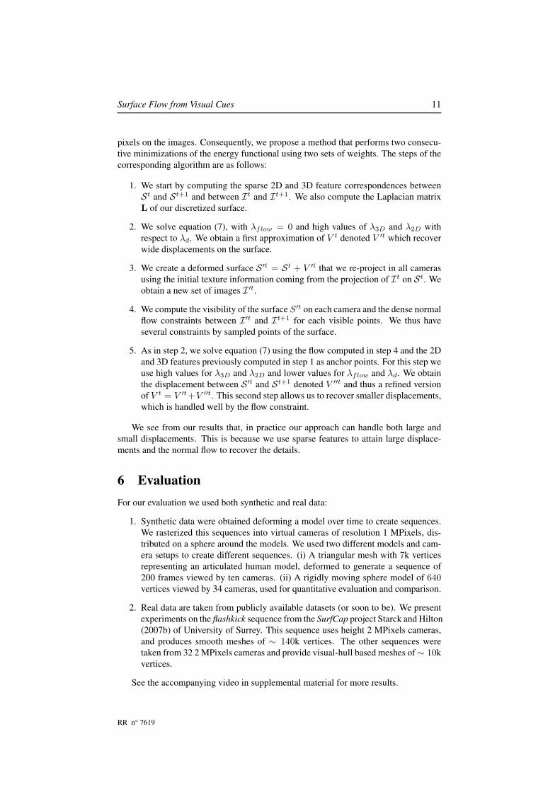
pixels on the images. Consequently, we propose a method that performs two consecu-tive minimizations of the energy functional using two sets of weights. The steps of thecorresponding algorithm are as follows:

1. We start by computing the sparse 2D and 3D feature correspondences betweenSt and St+1 and between It and It+1. We also compute the Laplacian matrixL of our discretized surface.

2. We solve equation (7), with λflow = 0 and high values of λ3D and λ2D withrespect to λd. We obtain a first approximation of V t denoted V ′t which recoverwide displacements on the surface.

3. We create a deformed surface S ′t = St + V ′t that we re-project in all camerasusing the initial texture information coming from the projection of It on St. Weobtain a new set of images I ′t.

4. We compute the visibility of the surface S′t on each camera and the dense normalflow constraints between I ′t and It+1 for each visible points. We thus haveseveral constraints by sampled points of the surface.

5. As in step 2, we solve equation (7) using the flow computed in step 4 and the 2Dand 3D features previously computed in step 1 as anchor points. For this step weuse high values for λ3D and λ2D and lower values for λflow and λd. We obtainthe displacement between S ′t and St+1 denoted V ′′t and thus a refined versionof V t = V ′t +V ′′t. This second step allows us to recover smaller displacements,which is handled well by the flow constraint.

We see from our results that, in practice our approach can handle both large andsmall displacements. This is because we use sparse features to attain large displace-ments and the normal flow to recover the details.

6 EvaluationFor our evaluation we used both synthetic and real data:

1. Synthetic data were obtained deforming a model over time to create sequences.We rasterized this sequences into virtual cameras of resolution 1 MPixels, dis-tributed on a sphere around the models. We used two different models and cam-era setups to create different sequences. (i) A triangular mesh with 7k verticesrepresenting an articulated human model, deformed to generate a sequence of200 frames viewed by ten cameras. (ii) A rigidly moving sphere model of 640vertices viewed by 34 cameras, used for quantitative evaluation and comparison.

2. Real data are taken from publicly available datasets (or soon to be). We presentexperiments on the flashkick sequence from the SurfCap project Starck and Hilton(2007b) of University of Surrey. This sequence uses height 2 MPixels cameras,and produces smooth meshes of ∼ 140k vertices. The other sequences weretaken from 32 2 MPixels cameras and provide visual-hull based meshes of∼ 10kvertices.

See the accompanying video in supplemental material for more results.

RR n° 7619


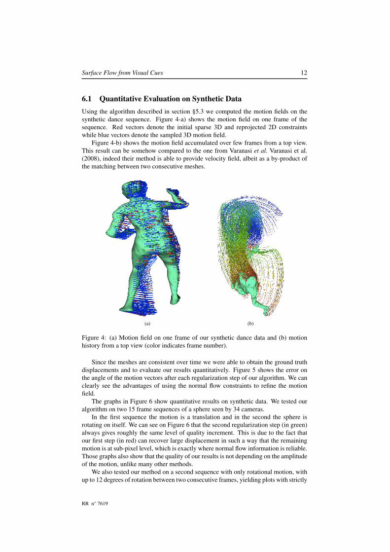
6.1 Quantitative Evaluation on Synthetic DataUsing the algorithm described in section §5.3 we computed the motion fields on thesynthetic dance sequence. Figure 4-a) shows the motion field on one frame of thesequence. Red vectors denote the initial sparse 3D and reprojected 2D constraintswhile blue vectors denote the sampled 3D motion field.

Figure 4-b) shows the motion field accumulated over few frames from a top view.This result can be somehow compared to the one from Varanasi et al. Varanasi et al.(2008), indeed their method is able to provide velocity field, albeit as a by-product ofthe matching between two consecutive meshes.

(a) (b)

Figure 4: (a) Motion field on one frame of our synthetic dance data and (b) motionhistory from a top view (color indicates frame number).

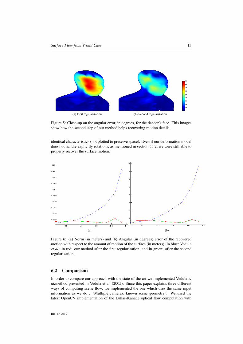
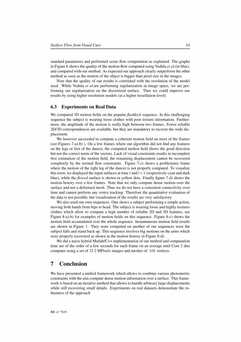
Since the meshes are consistent over time we were able to obtain the ground truthdisplacements and to evaluate our results quantitatively. Figure 5 shows the error onthe angle of the motion vectors after each regularization step of our algorithm. We canclearly see the advantages of using the normal flow constraints to refine the motionfield.

The graphs in Figure 6 show quantitative results on synthetic data. We tested ouralgorithm on two 15 frame sequences of a sphere seen by 34 cameras.

In the first sequence the motion is a translation and in the second the sphere isrotating on itself. We can see on Figure 6 that the second regularization step (in green)always gives roughly the same level of quality increment. This is due to the fact thatour first step (in red) can recover large displacement in such a way that the remainingmotion is at sub-pixel level, which is exactly where normal flow information is reliable.Those graphs also show that the quality of our results is not depending on the amplitudeof the motion, unlike many other methods.

We also tested our method on a second sequence with only rotational motion, withup to 12 degrees of rotation between two consecutive frames, yielding plots with strictly

RR n° 7619


(a) First regularization (b) Second regularization

Figure 5: Close-up on the angular error, in degrees, for the dancer’s face. This imagesshow how the second step of our method helps recovering motion details.

identical characteristics (not plotted to preserve space). Even if our deformation modeldoes not handle explicitly rotations, as mentioned in section §5.2, we were still able toproperly recover the surface motion.

(a) (b)

Figure 6: (a) Norm (in meters) and (b) Angular (in degrees) error of the recoveredmotion with respect to the amount of motion of the surface (in meters). In blue: Vedulaet al., in red: our method after the first regularization, and in green: after the secondregularization.

6.2 ComparisonIn order to compare our approach with the state of the art we implemented Vedula etal.method presented in Vedula et al. (2005). Since this paper explains three differentways of computing scene flow, we implemented the one which uses the same inputinformation as we do : "Multiple cameras, known scene geometry". We used thelatest OpenCV implementation of the Lukas-Kanade optical flow computation with

RR n° 7619


standard parameters and performed scene flow computation as explained. The graphsin Figure 6 shows the quality of the motion flow computed using Vedula et al.(in blue),and compared with our method. As expected our approach clearly outperform the othermethod as soon as the motion of the object is bigger than pixel size in the images.

Note that the quality of our results is correlated with the resolution of the modelused. While Vedula et al.are performing regularization in image space, we are per-forming our regularization on the discretized surface. Thus we could improve ourresults by using higher resolution models (at a higher tessellation level).

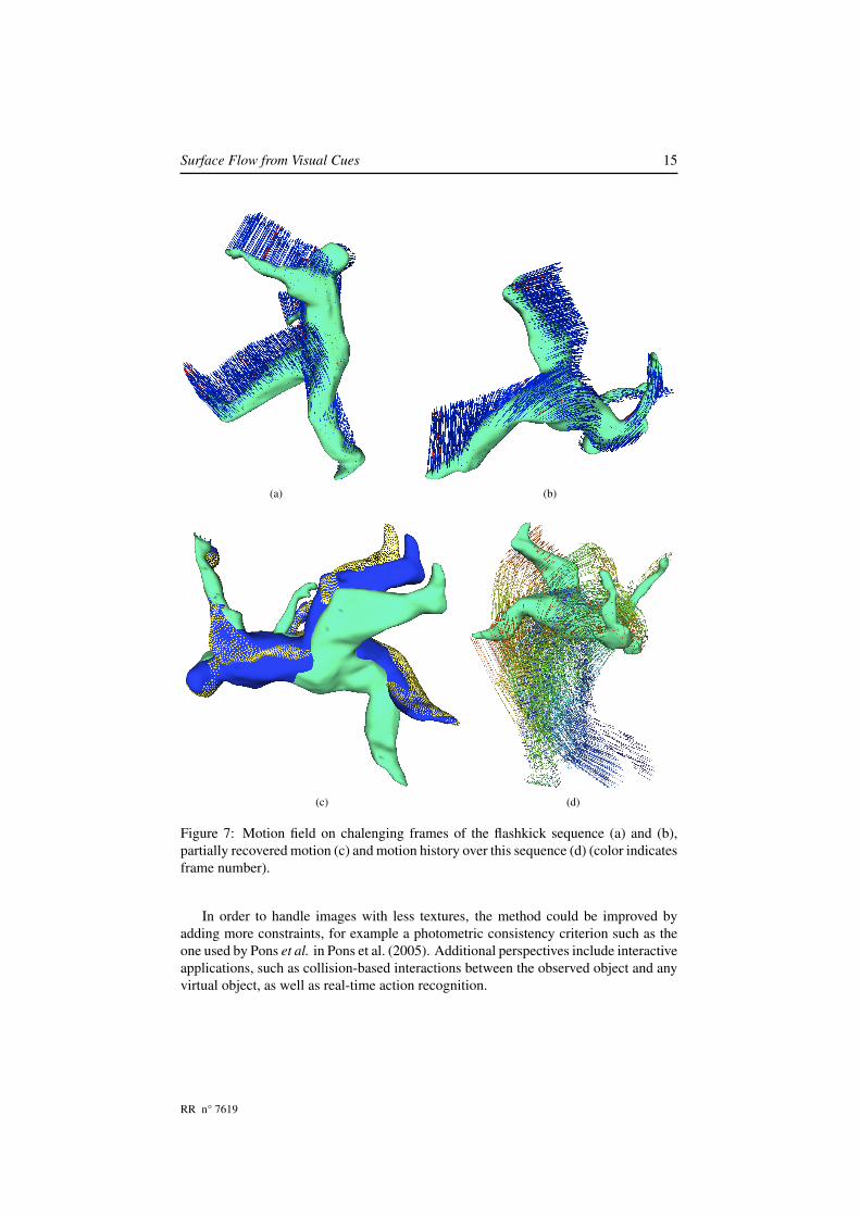
6.3 Experiments on Real DataWe computed 3D motion fields on the popular flashkick sequence. In this challengingsequence the subject is wearing loose clothes with poor texture information. Further-more, the amplitude of the motion is really high between two frames. Fewer reliable2D/3D correspondences are available, but they are mandatory to recover the wide dis-placement.

We however succeeded to compute a coherent motion field on most of the frames(see Figures 7-a)-b) ). On a few frames where our algorithm did not find any featureson the legs or feet of the dancer, the computed motion field shows the good directionbut not the correct norm of the vectors. Lack of visual constraints results in incompletefirst estimation of the motion field, the remaining displacement cannot be recoveredcompletely by the normal flow constraints. Figure 7-c) shows a problematic framewhere the motion of the right leg of the dancer is not properly computed. To visualizethis error, we displayed the input surfaces at time t and t+1 (respectively cyan and darkblue), while the flowed surface is shown in yellow dots. Finally figure 7-d) shows themotion history over a few frames. Note that we only compute dense motion over thesurface and not a deformed mesh. Thus we do not have a consistent connectivity overtime and cannot perform any vertex tracking. Therefore the quantitative evaluation ofthe data is not possible, but visualization of the results are very satisfactory.

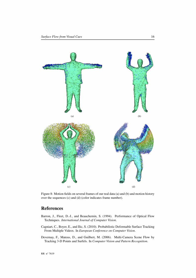
We also used our own sequences. One shows a subject performing a simple action,moving both hands from hips to head. The subject is wearing loose and highly texturesclothes which allow to compute a high number of reliable 2D and 3D features, seeFigure 8-a)-b) for examples of motion fields on this sequence. Figure 8-c) shows themotion field accumulated over the whole sequence. Instantaneous motion field resultsare shown in Figure 1. They were computed on another of our sequences were thesubject falls and stand back up. This sequence involves big motions on the arms whichwere properly recovered as shown in the motion history in Figure 8-d).

We did a naive hybrid Matlab/C++ implementation of our method and computationtime are of the order of a few seconds for each frame on an average intel Core 2 duocomputer using a set of 32 2 MPixels images and meshes of 10k vertices.

7 ConclusionWe have presented a unified framework which allows to combine various photometricconstraints with the aim compute dense motion information over a surface. This frame-work is based on an iterative method that allows to handle arbitrary large displacementswhile still recovering small details. Experiments on real datasets demonstrate the ro-bustness of the approach

RR n° 7619


(a) (b)

(c) (d)

Figure 7: Motion field on chalenging frames of the flashkick sequence (a) and (b),partially recovered motion (c) and motion history over this sequence (d) (color indicatesframe number).

In order to handle images with less textures, the method could be improved byadding more constraints, for example a photometric consistency criterion such as theone used by Pons et al. in Pons et al. (2005). Additional perspectives include interactiveapplications, such as collision-based interactions between the observed object and anyvirtual object, as well as real-time action recognition.

RR n° 7619


(a) (b)

(c) (d)

Figure 8: Motion fields on several frames of our real data (a) and (b) and motion historyover the sequences (c) and (d) (color indicates frame number).

ReferencesBarron, J., Fleet, D.-J., and Beauchemin, S. (1994). Performance of Optical Flow

Techniques. International Journal of Computer Vision.

Cagniart, C., Boyer, E., and Ilic, S. (2010). Probabilistic Deformable Surface TrackingFrom Multiple Videos. In European Conference on Computer Vision.

Devernay, F., Mateus, D., and Guilbert, M. (2006). Multi-Camera Scene Flow byTracking 3-D Points and Surfels. In Computer Vision and Pattern Recognition.

RR n° 7619


Franco, J.-S. and Boyer, E. (2008). Efficient Polyhedral Modeling from Silhouettes.IEEE Transactions on Pattern Analysis and Machine Intelligence.

Furukawa, Y. and Ponce, J. (2006). Carved Visual Hulls for Image-Based Modeling.In European Conference on Computer Vision.

Horn, B. and Schunck, B. (1981). Determining Optical Flow. Artificial Intelligence.

Isard, M. and MacCormick, J. (2006). Dense Motion and Disparity Estimation viaLoopy Belief Propagation. In Asian Conference on Computer Vision.

Liu, C., Yuen, J., Torralba, A., Sivic, J., and Freeman, W. (2008). SIFT Flow: DenseCorrespondence across Different Scenes. In European Conference on ComputerVision.

Lowe, D. (2004). Distinctive Image Features from Scale-invariant Keypoints. Interna-tional Journal of Computer Vision.

Lucas, B. and Kanade, T. (1981). An Iterative Image Registration Technique withan Application to Stereo Vision. In International Joint Conference on ArtificialIntelligence.

Naveed, A., Theobalt, C., Rossl, C., Thurn, S., and Seidel, H. (2008). Dense Corre-spondence Finding for Parametrization-free Animation Reconstruction from Video.In Computer Vision and Pattern Recognition.

Neumann, J. and Aloimonos, Y. (2002). Spatio-Temporal Stereo Using Multi-Resolution Subdivision Surfaces. International Journal of Computer Vision.

Pons, J.-P., Keriven, R., and Faugeras, O. (2005). Modelling Dynamic Scenes by Reg-istering Multi-View Image Sequences. In Computer Vision and Pattern Recognition.

Sorkine, O. and Alexa, M. (2007). As-Rigid-As-Possible Surface Modeling. In Euro-graphics Symposium on Geometry Processing.

Starck, J. and Hilton, A. (2007a). Correspondence Labeling for Wide-Timeframe Free-Form Surface Matching. In European Conference on Computer Vision.

Starck, J. and Hilton, A. (2007b). Surface Capture for Performance-Based Animation.IEEE Computer Graphics and Applications.

Varanasi, K., Zaharescu, A., Boyer, E., and Horaud, R. P. (2008). Temporal SurfaceTracking Using Mesh Evolution. In European Conference on Computer Vision.

Vedula, S., Baker, S., Rander, P., Collins, R., and Kanade, T. (2005). Three-Dimensional Scene Flow. IEEE Transactions on Pattern Analysis and Machine In-telligence.

Wedel, A., Rabe, C., Vaudrey, T., Brox, T., Franke, U., and Cremeres, D. (2008). Effi-cient Dense Scene Flow from Sparse or Dense Stereo Data. In European Conferenceon Computer Vision.

Xu, L., Jia, J., and Matsushita, Y. (2010). Motion Detail Preserving Optical FlowEstimation. In Computer Vision and Pattern Recognition.

RR n° 7619


Zaharescu, A., Boyer, E., Varanasi, K., and Horaud, R. P. (2009). Surface FeatureDetection and Description with Applications to Mesh Matching. In Computer Visionand Pattern Recognition.

Zhang, Y. and Kambhamettu, C. (2001). On 3D Scene Flow and Structure Estimation.In Computer Vision and Pattern Recognition.

RR n° 7619

Centre de recherche INRIA Grenoble – Rhône-Alpes655, avenue de l’Europe - 38334 Montbonnot Saint-Ismier (France)

Centre de recherche INRIA Bordeaux – Sud Ouest : Domaine Universitaire - 351, cours de la Libération - 33405 Talence CedexCentre de recherche INRIA Lille – Nord Europe : Parc Scientifique de la Haute Borne - 40, avenue Halley - 59650 Villeneuve d’Ascq

Centre de recherche INRIA Nancy – Grand Est : LORIA, Technopôle de Nancy-Brabois - Campus scientifique615, rue du Jardin Botanique - BP 101 - 54602 Villers-lès-Nancy Cedex

Centre de recherche INRIA Paris – Rocquencourt : Domaine de Voluceau - Rocquencourt - BP 105 - 78153 Le Chesnay CedexCentre de recherche INRIA Rennes – Bretagne Atlantique : IRISA, Campus universitaire de Beaulieu - 35042 Rennes Cedex

Centre de recherche INRIA Saclay – Île-de-France : Parc Orsay Université - ZAC des Vignes : 4, rue Jacques Monod - 91893 Orsay CedexCentre de recherche INRIA Sophia Antipolis – Méditerranée : 2004, route des Lucioles - BP 93 - 06902 Sophia Antipolis Cedex

ÉditeurINRIA - Domaine de Voluceau - Rocquencourt, BP 105 - 78153 Le Chesnay Cedex (France)

http://www.inria.frISSN 0249-6399

Documents

Surface Flow from Visual Cues - hal.inria.fr · Flot de surface à partir d’indices visuels ... Dans cette optique, ... and Kanade (1981) have been proposed