Embed Size (px)
Citation preview
HAL Id: inria-00277995https://hal.inria.fr/inria-00277995v2
Submitted on 14 May 2008
HAL is a multi-disciplinary open accessarchive for the deposit and dissemination of sci-entific research documents, whether they are pub-lished or not. The documents may come fromteaching and research institutions in France orabroad, or from public or private research centers.
L’archive ouverte pluridisciplinaire HAL, estdestinée au dépôt et à la diffusion de documentsscientifiques de niveau recherche, publiés ou non,émanant des établissements d’enseignement et derecherche français ou étrangers, des laboratoirespublics ou privés.
Computation Tree Regular Logic for Genetic RegulatoryNetworks
Radu Mateescu, Pedro Monteiro, Estelle Dumas, Hidde de Jong
To cite this version:Radu Mateescu, Pedro Monteiro, Estelle Dumas, Hidde de Jong. Computation Tree Regular Logic forGenetic Regulatory Networks. [Research Report] RR-6521, INRIA. 2008, pp.53. �inria-00277995v2�
appor t de r ech er ch e
ISS
N02
49-6
399
ISR
NIN
RIA
/RR
--65
21--
FR
+E
NG
Th„emes BIO et COM
INSTITUT NATIONAL DE RECHERCHE EN INFORMATIQUE ET EN AUTOMATIQUE
Computation Tree Regular Logic forGenetic Regulatory Networks
Radu Mateescu — Pedro T. Monteiro —
Estelle Dumas — Hidde de Jong
N° 6521
Mai 2008

Centre de recherche INRIA Grenoble – Rhône-AlpesInovallée, 655, avenue de l’Europe, Montbonnot, 38334 Saint Ismier Cedex (France)
Téléphone : +33 4 76 61 52 00 — Télécopie +33 4 76 61 52 52
Computation Tree Regular Logic for
Genetic Regulatory Networks
Radu Mateescu* , Pedro T. Monteiro** ,
Estelle Dumas*** , Hidde de Jong****
Themes BIO et COM — Systemes biologiques et Systemes communicants
Projets Ibis et Vasy
Rapport de recherche n° 6521 — Mai 2008 — 53 pages
Abstract: Model checking has proven to be a useful analysis technique not only for concur-rent systems, but also for the genetic regulatory networks (Grns) that govern the functioningof living cells. The applications of model checking in systems biology have revealed that tem-poral logics should be able to capture both branching-time and fairness properties (neededfor specifying multistability and oscillation properties, respectively). At the same time, theyshould have a user-friendly syntax easy to employ by non-experts. In this report, we defineComputation Tree Regular Logic (Ctrl), an extension of Ctl with regular expressions andfairness operators that attempts to match these criteria. Ctrl subsumes both Ctl andLtl, and has a reduced set of temporal operators indexed by regular expressions, inspiredfrom the modalities of Propositional Dynamic Logic (Pdl). We also develop a translationof Ctrl into Hennessy-Milner Logic with Recursion (HmlR), an equational variant of themodal µ-calculus. This has allowed us to obtain an on-the-fly model checker with diagnosticfor Ctrl by directly reusing the verification technology available in the Cadp toolbox. Weillustrate the application of the Ctrl model checker by analyzing the Grn controlling thecarbon starvation response of Escherichia coli.
Key-words: genetic regulatory networks, model checking, system biology, temporal logic,verification
* [email protected]** [email protected]
*** [email protected]**** [email protected]
Logique reguliere du temps arborescent
pour les reseaux de regulation genique
Resume : La verification par logique temporelle (model checking) s’est revelee comme etantune technique d’analyse utile non seulement pour les systemes concurrents, mais egalementpour les reseaux de regulation genique (Rrgs) qui gouvernent le fonctionnement des cel-lules vivantes. Les applications du model checking en biologie systemique ont souligne lefait que les logiques temporelles utilisees devraient capturer a la fois des aspects arbores-cents et d’equite (necessaires pour specifier des proprietes de multistabilite et respectivementd’oscillation), tout en ayant une syntaxe simple et intuitive, facile d’emploi pour les non-specialistes. Dans ce rapport, nous definissons Computation Tree Regular Logic (Ctrl),une extension de Ctl avec des expressions regulieres et des operateurs d’equite qui visea repondre a ces criteres. Ctrl subsume a la fois Ctl et Ltl, et possede un ensemblereduit d’operateurs temporels indexes par des expressions regulieres, inspires des modalitesde Propositional Dynamic Logic (Pdl). Nous definissons egalement une traduction de Ctrlvers la logique de Hennessy-Milner avec recursion (HmlR), une variante equationnelle duµ-calcul modal, qui a permis d’obtenir un evaluateur a la volee avec diagnostic pour Ctrl enreutilisant directement la technologie de verification disponible dans la boıte a outils Cadp.Nous illustrons l’application de l’evaluateur pour Ctrl avec l’exemple du Rrg controlantla reponse au manque de carbone chez Escherichia coli.
Mots-cles : reseaux de regulation genique, model checking, biologie systemique, logiquetemporelle, verification
Computation Tree Regular Logic for Genetic Regulatory Networks 3
1 Introduction
Explicit state verification has been mostly applied to the analysis of concurrent systems in en-gineering. Recently, however, biological regulatory networks have been recognized as specialcases of concurrent systems as well, which has opened the way for the application of formalverification technology in the emerging field of systems biology (see [29, 54] for reviews).The networks controlling cellular functions consist of genes, proteins, small molecules, andtheir mutual interactions. Most of these networks are large and complex, thus defying ourcapacity to understand how the dynamic behavior of the cell emerges from the structure ofinteractions. A large number of mathematical formalisms have been proposed to describethese networks [23], giving rise to models that can be directly or indirectly mapped to Kripkestructures.
The representation of the dynamics of biological regulatory networks by means of Kripkestructures enables the application of formal verification techniques to the analysis of proper-ties of the networks. In particular, such properties can be formulated as queries in temporallogic, and verified by means of model checking algorithms on the Kripke structures. Exam-ples of the kind of properties that biologists are interested in include the following:� Is the basal glycerol production level combined with rapid closure of Fps1 sufficient to
explain an initial glycerol accumulation after osmotic shock? [43]� Once a cell has executed Start, does it slip back into G1 phase and repeat Start?Or rather, must it execute a Finish to return to G1? [19].� Does Shc phosphorylation exhibit a relative acceleration with decreasing Egf concen-tration and show a decline over time? [56]
Several applications of model checking exists in the bioinformatics and systems biology lit-erature [3, 6, 10, 13, 16, 17, 30]. In our previous work [8, 10], we have developed GeneticNetwork Analyzer (Gna), a tool for the qualitative simulation of genetic regulatory networks,and connected it to state-of-the-art model checkers like NuSmv [20] and Cadp [33].
All of the above approaches express the properties of interest in classical temporal logics likeCtl [21] and Ltl [48]. The application to actual biological systems brought a few propertiesof the network dynamics to the fore that are not easily expressed in these logics. For in-stance, questions about multistability are important in the analysis of biological regulatorynetworks [59], but difficult (or impossible) to express in Ltl. Ctl is capable of dealingwith branching time, important for multistability and other properties of non-deterministicmodels. However, it does not do a good job when faced with questions about cycles in aKripke structure. Such cycles may correspond to sustained or damped oscillations in the con-centration of molecular species, underlying cellular rhythms [19, 47]. Ctl is not expressiveenough to specify the occurrence of oscillations of indefinite length, a special kind of fairnessproperty [10]. An obvious solution would be to consider Ctl∗ [26] or the propositional µ-calculus [44], both of which subsume Ctl and Ltl; however, these powerful branching-timelogics are complex to understand and use by non-experts. More generally, it is not easy
RR n° 6521
4 Mateescu, Monteiro, Dumas & de Jong
to express observations in temporal logic. Often these take the form of patterns of eventscorresponding to variations of system parameters (protein concentrations, their derivatives,etc.), which can be compared with the model predictions and thus help validate the model.Observations are conveniently and concisely formulated in terms of regular expressions, butthese are not provided by standard temporal logics such as Ctl and Ltl.
In this report, we aim at providing a temporal specification language that allows expressingproperties of biological interest and strikes a suitable compromise between expressive power,user-friendliness, and complexity of model checking. In order to achieve this objective, wepropose a specification language named Ctrl (Computation Tree Regular Logic), which ex-tends Ctl with regular expressions and fairness operators. Ctrl is more expressive thanprevious extensions of Ctl with regular expressions, such as Rctl [12] and RegCtl [14],whilst having a simpler syntax due to a different choice of primitive temporal operators,inspired from dynamic logics like Pdl [28]. Ctrl also subsumes Ctl, Ltl, and Pdl-∆ [57]allowing in particular the concise expression of bistability and oscillation properties. Al-though Ctrl was primarily designed for describing properties of regulatory networks insystem biology, it also enables a succinct formulation of typical safety, liveness, and fairnessproperties useful for the verification of concurrent systems in other domains.
As regards the evaluation of Ctrl formulas on Kripke structures, we attempt to avoid theeffort of building a model checker from scratch by reusing as much as possible existing verifi-cation technology. We adopt as verification engine Cadp [33], a state-of-the-art verificationtoolbox for concurrent asynchronous systems that provides, among other functionalities, on-the-fly model checking and diagnostic generation for µ-calculus formulas on labeled transitionsystems (Ltss). In order to reuse this technology, we have to move from the state-based set-ting (Ctrl and Kripke structures) to the action-based setting (µ-calculus and Ltss). Thetranslation from Kripke structures to Ltss is done in the standard way [21], simply by mi-grating information from states to transition labels without changing the structure of themodel, i.e., keeping the same states and transition relations. The translation from Ctrl toan action-based logic is carried out by considering as target language HmlR [46], an alter-native equational representation of the modal µ-calculus which is also accepted as input bythe Evaluator 3.6 [51] model checker of Cadp. HmlR yields a more succinct translationthan plain µ-calculus due to the possibility of factoring out common subformulas using fixedpoint equations. Moreover, the equational representation of HmlR is closer to the booleanequation systems (Bess) used as intermediate formalism by the verification engine, namelythe Cæsar Solve [50] generic library for local Bes resolution. Once the translator fromCtrl to HmlR is available, its connection with Evaluator 3.6 results in the immediateavailability of an on-the-fly model checker equipped with full diagnostic features (generationof examples and counterexamples).
The Ctrl model checking procedure obtained in this way has a linear-time complexityw.r.t. the size of the formula and the Kripke structure for a significant part of the logic.This part notably subsumes Pdl-∆ and allows the multistability and oscillation propertiesto be captured. The inevitability operator of Ctrl and its infinitary version (inevitablelooping) has an exponential worst-case complexity w.r.t. the size of its regular subformula;this complexity becomes linear, however, when the regular subformula is “deterministic” in
INRIA
Computation Tree Regular Logic for Genetic Regulatory Networks 5
a way similar to finite automata. In practice, the usage of Ctrl and the model checkerreveals that properties of biological interest can be expressed and verified efficiently. Weillustrate this on the analysis of a model of the regulatory network (Grn) controlling thecarbon starvation response of E. coli.
Report outline. Section 2 defines the syntax and semantics of Ctrl and discusses itsexpressiveness w.r.t. existing widely-used logics. Section 2.4 defines the regular equationsystems (Ress), an intermediate equational form into which Ctrl formulas will be trans-lated. Sections 3.1 and 3.2 present the translations from Ctrl to Ress and then to modalequation systems (Mess). Section 4 formulates the model checking of a Mes on a Kripkestructure as the resolution of a boolean equation system (Bes). We show how this is per-formed on-the-fly using specialized algorithms and indicate the complexity of the modelchecking procedure. Section 5 describes the implementation of the Ctrl model checker inconnection with Cadp and illustrates its application on the example of E. coli . Section 6provides some concluding remarks and directions for future work. Appendix A contains theproofs of the translation phases from Ctrl to Mess.
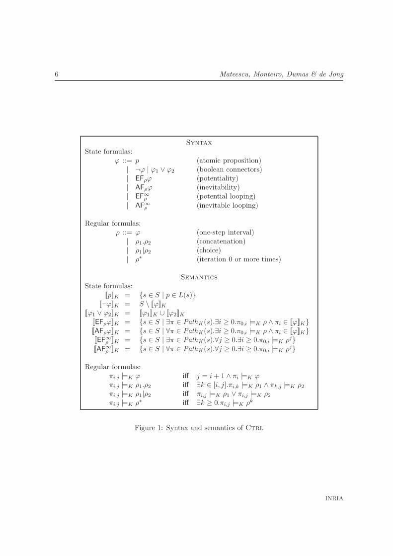
2 Syntax and Semantics
2.1 Computation Tree Regular Logic
Ctrl is interpreted on Kripke structures, which provide a natural formal description ofconcurrent systems, including biological regulatory networks. A Kripke structure is a tupleK = 〈S,P,L, T, s0〉, where: S is the set of states; P is a set of atomic propositions (predicatesover states); L : S → 2P is the state labeling (each state s is associated with the atomicpropositions satisfied by s); T ⊆ S × S is the transition relation; and s0 ∈ S is the initialstate. Transitions (s1, s2) ∈ T are also noted s1 →T s2 (the subscript T is omitted if it isclear from the context). The transition relation T is assumed to be total, i.e., for each states1 ∈ S, there exists a transition s1 →T s2. A path π = s0s1 . . . sk . . . is an infinite sequenceof states such that si →T si+1 for every i ≥ 0. The i-th state of a path π is noted πi. Theinterval going from the i-th state of a path π to the j-th state of π inclusively (where i ≤ j)is noted πi,j. An interval π0,i is called prefix of π. For each state s ∈ S, Path(s) denotesthe set of all paths going out of s, i.e., the paths π such that π0 = s. In the sequel, weassume the existence of a Kripke structure K = 〈S,P,L, T, s0〉, on which all formulas willbe interpreted.
The syntax and semantics of Ctrl are defined in Figure 1. The logic contains two kinds ofentities: state formulas (noted ϕ) and regular formulas (noted ρ), which characterize prop-erties of states and intervals, respectively. State formulas are built from atomic propositionsp ∈ P by using standard boolean operators and the EF, AF, EF∞, AF∞ temporal operatorsindexed by regular formulas ρ. Regular formulas are built from state formulas by usingstandard regular expression operators.
RR n° 6521
6 Mateescu, Monteiro, Dumas & de Jong
SyntaxState formulas:
ϕ ::= p (atomic proposition)| ¬ϕ | ϕ1 ∨ ϕ2 (boolean connectors)| EFρϕ (potentiality)| AFρϕ (inevitability)| EF∞
ρ (potential looping)
| AF∞ρ (inevitable looping)
Regular formulas:ρ ::= ϕ (one-step interval)
| ρ1.ρ2 (concatenation)| ρ1|ρ2 (choice)| ρ∗ (iteration 0 or more times)
SemanticsState formulas:
[[p]]K = {s ∈ S | p ∈ L(s)}[[¬ϕ]]K = S \ [[ϕ]]K
[[ϕ1 ∨ ϕ2]]K = [[ϕ1]]K ∪ [[ϕ2]]K[[EFρϕ]]K = {s ∈ S | ∃π ∈ PathK(s).∃i ≥ 0.π0,i |=K ρ ∧ πi ∈ [[ϕ]]K}[[AFρϕ]]K = {s ∈ S | ∀π ∈ PathK(s).∃i ≥ 0.π0,i |=K ρ ∧ πi ∈ [[ϕ]]K}[[EF∞
ρ ]]K = {s ∈ S | ∃π ∈ PathK(s).∀j ≥ 0.∃i ≥ 0.π0,i |=K ρj}[[AF∞
ρ ]]K = {s ∈ S | ∀π ∈ PathK(s).∀j ≥ 0.∃i ≥ 0.π0,i |=K ρj}
Regular formulas:πi,j |=K ϕ iff j = i+ 1 ∧ πi |=K ϕπi,j |=K ρ1.ρ2 iff ∃k ∈ [i, j].πi,k |=K ρ1 ∧ πk,j |=K ρ2
πi,j |=K ρ1|ρ2 iff πi,j |=K ρ1 ∨ πi,j |=K ρ2
πi,j |=K ρ∗ iff ∃k ≥ 0.πi,j |=K ρk
Figure 1: Syntax and semantics of Ctrl
INRIA
Computation Tree Regular Logic for Genetic Regulatory Networks 7
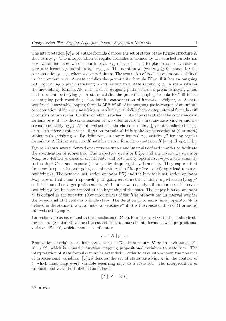
The interpretation [[ϕ]]K of a state formula denotes the set of states of the Kripke structure Kthat satisfy ϕ. The interpretation of regular formulas is defined by the satisfaction relation|=K , which indicates whether an interval πi,j of a path in a Kripke structure K satisfiesa regular formula ρ (notation πi,j |=K ρ). The notation ρj (where j ≥ 0) stands for theconcatenation ρ . . . ρ, where ρ occurs j times. The semantics of boolean operators is definedin the standard way. A state satisfies the potentiality formula EFρϕ iff it has an outgoingpath containing a prefix satisfying ρ and leading to a state satisfying ϕ. A state satisfiesthe inevitability formula AFρϕ iff all of its outgoing paths contain a prefix satisfying ρ andlead to a state satisfying ϕ. A state satisfies the potential looping formula EF∞
ρ iff it hasan outgoing path consisting of an infinite concatenation of intervals satisfying ρ. A statesatisfies the inevitable looping formula AF∞
ρ iff all of its outgoing paths consist of an infiniteconcatenation of intervals satisfying ρ. An interval satisfies the one-step interval formula ϕ iffit consists of two states, the first of which satisfies ϕ. An interval satisfies the concatenationformula ρ1.ρ2 if it is the concatenation of two subintervals, the first one satisfying ρ1 and thesecond one satisfying ρ2. An interval satisfies the choice formula ρ1|ρ2 iff it satisfies either ρ1,or ρ2. An interval satisfies the iteration formula ρ∗ iff it is the concatenation of (0 or more)subintervals satisfying ρ. By definition, an empty interval πi,i satisfies ρ0 for any regularformula ρ. A Kripke structure K satisfies a state formula ϕ (notation K |= ϕ) iff s0 ∈ [[ϕ]]K .
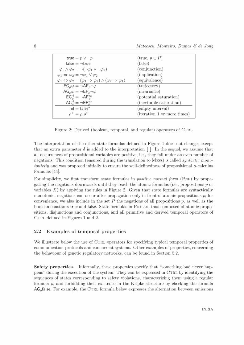
Figure 2 shows several derived operators on states and intervals defined in order to facilitatethe specification of properties. The trajectory operator EGρϕ and the invariance operatorAGρϕ are defined as duals of inevitability and potentiality operators, respectively, similarlyto the their Ctl counterparts (obtained by dropping the ρ formulas). They express thatfor some (resp. each) path going out of a state, all of its prefixes satisfying ρ lead to statessatisfying ϕ. The potential saturation operator EG⊣
ρ and the inevitable saturation operator
AG⊣ρ express that some (resp. each) path going out of a state contains a prefix satisfying ρ∗
such that no other larger prefix satisfies ρ∗; in other words, only a finite number of intervalssatisfying ρ can be concatenated at the beginning of the path. The empty interval operatornil is defined as the iteration (0 or more times) of the false proposition; an interval satisfiesthe formula nil iff it contains a single state. The iteration (1 or more times) operator ‘+’ isdefined in the standard way; an interval satisfies ρ+ iff it is the concatenation of (1 or more)intervals satisfying ρ.
For technical reasons related to the translation of Ctrl formulas to Mess in the model check-ing process (Section 3), we need to extend the grammar of state formulas with propositionalvariables X ∈ X , which denote sets of states:
ϕ ::= X | p | . . .
Propositional variables are interpreted w.r.t. a Kripke structure K by an environment δ :X → 2S , which is a partial function mapping propositional variables to state sets. Theinterpretation of state formulas must be extended in order to take into account the presenceof propositional variables: [[ϕ]]Kδ denotes the set of states satisfying ϕ in the context ofδ, which must map every variable occurring in ϕ to a state set. The interpretation ofpropositional variables is defined as follows:
[[X]]Kδ = δ(X)
RR n° 6521
8 Mateescu, Monteiro, Dumas & de Jong
true = p ∨ ¬p (true, p ∈ P )false = ¬true (false)
ϕ1 ∧ ϕ2 = ¬(¬ϕ1 ∨ ¬ϕ2) (conjunction)ϕ1 ⇒ ϕ2 = ¬ϕ1 ∨ ϕ2 (implication)ϕ1 ⇔ ϕ2 = (ϕ1 ⇒ ϕ2) ∧ (ϕ2 ⇒ ϕ1) (equivalence)
EGρϕ = ¬AFρ¬ϕ (trajectory)AGρϕ = ¬EFρ¬ϕ (invariance)EG⊣
ρ = ¬AF∞ρ (potential saturation)
AG⊣ρ = ¬EF∞
ρ (inevitable saturation)
nil = false∗ (empty interval)
ρ+ = ρ.ρ∗ (iteration 1 or more times)
Figure 2: Derived (boolean, temporal, and regular) operators of Ctrl
The interpretation of the other state formulas defined in Figure 1 does not change, exceptthat an extra parameter δ is added to the interpretation [[ ]]. In the sequel, we assume thatall occurrences of propositional variables are positive, i.e., they fall under an even number ofnegations. This condition (ensured during the translation to Mess) is called syntactic mono-tonicity and was proposed initially to ensure the well-definedness of propositional µ-calculusformulas [44].
For simplicity, we first transform state formulas in positive normal form (Pnf) by propa-gating the negations downwards until they reach the atomic formulas (i.e., propositions p orvariables X) by applying the rules in Figure 2. Given that state formulas are syntacticallymonotonic, negations can occur after propagation only in front of atomic propositions p; forconvenience, we also include in the set P the negations of all propositions p, as well as theboolean constants true and false. State formulas in Pnf are thus composed of atomic propo-sitions, disjunctions and conjunctions, and all primitive and derived temporal operators ofCtrl defined in Figures 1 and 2.
2.2 Examples of temporal properties
We illustrate below the use of Ctrl operators for specifying typical temporal properties ofcommunication protocols and concurrent systems. Other examples of properties, concerningthe behaviour of genetic regulatory networks, can be found in Section 5.2.
Safety properties. Informally, these properties specify that “something bad never hap-pens” during the execution of the system. They can be expressed in Ctrl by identifying thesequences of states corresponding to safety violations, characterizing them using a regularformula ρ, and forbidding their existence in the Kripke structure by checking the formulaAGρfalse. For example, the Ctrl formula below expresses the alternation between emissions
INRIA
Computation Tree Regular Logic for Genetic Regulatory Networks 9
and receptions of messages in a communication protocol that behaves as a one-slot buffer:
AG((nil | (true∗.rcv)).(¬snd )∗.rcv) | (true∗.snd .(¬rcv)∗.snd)false
where the atomic propositions snd and rcv indicate the emission and reception of a message,respectively. The first alternative in the regular subformula above forbids the occurrence ofa reception before the first message was emitted and also the occurrence of two consecutivereceptions without an emission in between. The second alternative requires that a receptionmust occur between every two consecutive emissions.
This property can also be specified in Ctl using 5 temporal operators:
¬E[¬snd U rcv ] ∧ AG(rcv ⇒ ¬E[¬snd U rcv ]) ∧ AG(snd ⇒ ¬E[¬rcv U snd ])
where AG ϕ = ¬E[true U ¬ϕ] is the invariance operator of Ctl.
Liveness properties. Informally, these properties specify that “something good even-tually happens” during the execution of the system. They can be expressed in Ctrl bycapturing the desirable sequences of states, characterizing them using a regular formula ρ,and expressing their potential or inevitable presence in the Kripke structure by means ofthe EFρ and AFρ operators, respectively. For instance, the Ctrl property below states thatevery time a message is emitted, then it will be eventually received after a finite number oftransmission errors:
AGtrue∗.sndAF(true∗.err)∗.rcv true
This property cannot be specified in Ctl because of the presence of two nested ∗ operatorsin the regular subformula of the AF operator.
Fairness properties. Informally, these properties specify the progression of all the con-current processes present in the system, which may be competing for the access to sharedresources. In Ctrl, fairness properties can be expressed by identifying the infinite executionsequences denoting the starvation of a certain process, characterizing them using the EF∞
ρ
operator, and forbidding their presence in the Kripke structure. The Ctrl formula belowspecifies that after a process has requested the access to a shared resource, it cannot beindefinitely preempted in getting access to the resource by another process:
¬EFtrue∗.req1EF
∞(¬get1)∗.req2.(¬get1)∗.get2
where the atomic propositions req i and get i denote the request and the access of process ito the resource, respectively. An equivalent formulation of this property can be rewrittenby propagating the negation through the temporal operators using the dualities shown inFigure 2:
AGtrue∗.req1AG
⊣(¬get1)
∗.req2.(¬get1)∗.get2
This property cannot be expressed in Ctl because it involves the repetition of alternatingreq2 and get2, but can be expressed in Ltl using 5 temporal operators:
G(req1 ⇒ ((get1 R ¬req2) ∨ (¬get1 U ((req2 ∧ (get1 R ¬get2)) ∨ (get2 ∧ (get1 R ¬req2))))))
where ϕ1 R ϕ2 = ¬(¬ϕ1 U ¬ϕ2) is the release operator of Ltl.
RR n° 6521
10 Mateescu, Monteiro, Dumas & de Jong
2.3 Expressiveness
Ctrl is a natural extension of Ctl [21], whose main temporal operators can be describedusing the EF and AF operators of Ctrl as follows:
E[ϕ1 U ϕ2] = EFϕ∗
1ϕ2 A[ϕ1 U ϕ2] = AFϕ∗
1ϕ2
The until operator U of Ctl is not primitive in Ctrl; this is a difference w.r.t. otherextensions of Ctl, such as Rctl [12] and RegCtl [14], which keep the U operator primitiveas in the original logic.
Ctrl also subsumes Ltl [48], because the potential looping operator EF∞ is able to capturethe acceptance condition of Buchi automata. Assuming that the atomic proposition p char-acterizes the accepting states in a Buchi automaton (represented as a Kripke structure), theformula below expresses the existence of an infinite sequence passing infinitely often throughan accepting state:
EF∞true∗.p.true+
The + operator is necessary in order to avoid empty sequences consisting of a single statesatisfying p. Of course, the EF∞ operator does not allow a direct translation of the Ltloperators, but may serve as an intermediate form for model checking Ltl formulas; in thisrespect, this operator is similar to the “never claims” used for specifying properties in theearly versions of the Spin model checker [37].
Thus, Ctrl subsumes both Ctl and Ltl. This subsumption is strict, since these twologics are uncomparable w.r.t. their expressive power (i.e., each one can describe propertiesunexpressible in the other one) [21]. In fact, the Ctrl fragment containing the booleanconnectors and the temporal operators EF and EF∞ can be seen as a state-based variant ofPdl-∆ [57], which has been shown to be more expressive than Ctl∗ [62].
As regards other existing extensions of Ctl with regular operators, Ctrl subsumes RegCtl,whose U operator indexed by a regular formula can be expressed using the EF operator ofCtrl as follows:
E[ϕ1 Uρ ϕ2] = EFρ & ϕ∗
1ϕ2
The & operator stands for the intersection of regular formulas; although this operator is notpresent in Ctrl, its occurrence above can be expanded in terms of the regular operatorsavailable in Ctrl by applying the rules below:
ϕ′ & ϕ∗ = ϕ′ & ϕ (ρ1.ρ2) & ϕ∗ = (ρ1 & ϕ∗).(ρ2 & ϕ∗)(ρ1|ρ2) & ϕ∗ = (ρ1 & ϕ∗)|(ρ2 & ϕ∗) (ρ1
∗) & ϕ∗ = (ρ1 & ϕ∗)∗
The subsumption of RegCtl is strict because the U operator of RegCtl cannot describe aninfinite concatenation of intervals satisfying a regular formula ρ, which is specified in Ctrlusing the EF∞
ρ operator. In [14] it is shown that RegCtl is more expressive than Rctl [12],the extension of Ctl with regular expressions underlying the Sugar [11] specification lan-guage; consequently, Ctrl also subsumes Rctl.
INRIA
Computation Tree Regular Logic for Genetic Regulatory Networks 11
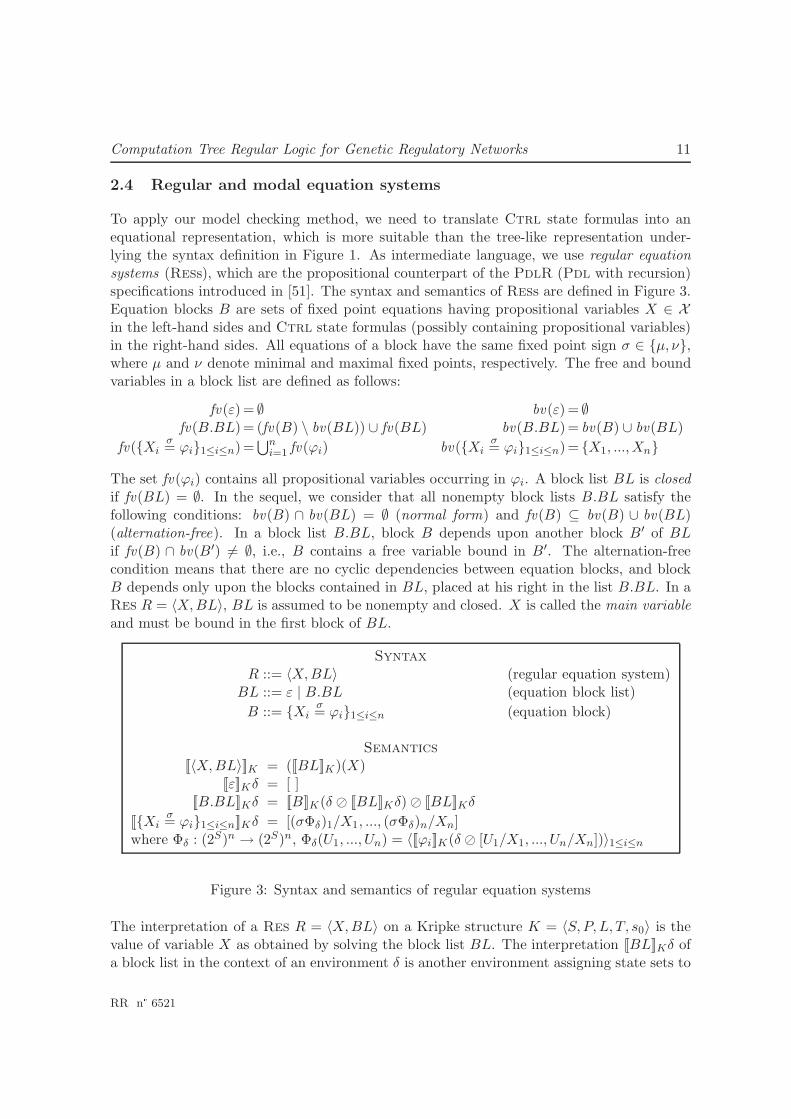
2.4 Regular and modal equation systems
To apply our model checking method, we need to translate Ctrl state formulas into anequational representation, which is more suitable than the tree-like representation under-lying the syntax definition in Figure 1. As intermediate language, we use regular equationsystems (Ress), which are the propositional counterpart of the PdlR (Pdl with recursion)specifications introduced in [51]. The syntax and semantics of Ress are defined in Figure 3.Equation blocks B are sets of fixed point equations having propositional variables X ∈ Xin the left-hand sides and Ctrl state formulas (possibly containing propositional variables)in the right-hand sides. All equations of a block have the same fixed point sign σ ∈ {µ, ν},where µ and ν denote minimal and maximal fixed points, respectively. The free and boundvariables in a block list are defined as follows:
fv(ε) = ∅ bv(ε) = ∅fv(B.BL)= (fv(B) \ bv(BL)) ∪ fv(BL) bv(B.BL)= bv(B) ∪ bv(BL)
fv({Xiσ= ϕi}1≤i≤n)=
⋃ni=1 fv(ϕi) bv({Xi
σ= ϕi}1≤i≤n)= {X1, ...,Xn}
The set fv(ϕi) contains all propositional variables occurring in ϕi. A block list BL is closedif fv(BL) = ∅. In the sequel, we consider that all nonempty block lists B.BL satisfy thefollowing conditions: bv(B) ∩ bv(BL) = ∅ (normal form) and fv(B) ⊆ bv(B) ∪ bv(BL)(alternation-free). In a block list B.BL, block B depends upon another block B′ of BLif fv(B) ∩ bv(B′) 6= ∅, i.e., B contains a free variable bound in B′. The alternation-freecondition means that there are no cyclic dependencies between equation blocks, and blockB depends only upon the blocks contained in BL, placed at his right in the list B.BL. In aRes R = 〈X,BL〉, BL is assumed to be nonempty and closed. X is called the main variableand must be bound in the first block of BL.
SyntaxR ::= 〈X,BL〉 (regular equation system)
BL ::= ε | B.BL (equation block list)
B ::= {Xiσ= ϕi}1≤i≤n (equation block)
Semantics[[〈X,BL〉]]K = ([[BL]]K)(X)
[[ε]]Kδ = [ ][[B.BL]]Kδ = [[B]]K(δ ⊘ [[BL]]Kδ) ⊘ [[BL]]Kδ
[[{Xiσ= ϕi}1≤i≤n]]Kδ = [(σΦδ)1/X1, ..., (σΦδ)n/Xn]
where Φδ : (2S)n → (2S)n, Φδ(U1, ..., Un) = 〈[[ϕi]]K(δ ⊘ [U1/X1, ..., Un/Xn])〉1≤i≤n
Figure 3: Syntax and semantics of regular equation systems
The interpretation of a Res R = 〈X,BL〉 on a Kripke structure K = 〈S,P,L, T, s0〉 is thevalue of variable X as obtained by solving the block list BL. The interpretation [[BL]]Kδ ofa block list in the context of an environment δ is another environment assigning state sets to
RR n° 6521
12 Mateescu, Monteiro, Dumas & de Jong
all variables bound in BL. Since the blocks of BL depend upon each other from left to right,the interpretation of BL can be defined inductively, by solving the blocks from right to left.The notation δ ⊘ [U1/X1, ..., Un/Xn] stands for the extension of δ with [U1/X1, ..., Un/Xn],i.e., an environment identical to δ except for variables X1, ...,Xn, which are mapped to thestate sets U1, ..., Un, respectively. The empty environment is noted [ ]. The interpretation ofan equation block B is the environment mapping the variables bound in B to the state setsgiven by the corresponding fixed point of the functional associated to the block. When BL isclosed, the δ environment is omitted. The state formulas in the right-hand sides of equationsare assumed to be syntactically monotonic, which according to Tarski’s theorem [58] ensuresthe well-definedness of the functionals associated to blocks.
A modal equation system (Mes) M = 〈X,BL〉 is a Res where all Ctrl temporal operatorsoccurring in the right-hand sides of equations contain only atomic regular formulas, i.e.,without any regular operator (‘.’, ‘|’, ‘∗’). Mess are the propositional counterpart of theHmlR (Hml with recursion) specifications, proposed in [46] as an equivalent equationaldefinition of the modal µ-calculus. In our setting, Mess are suitable as target language fortranslating Ctrl formulas, since they are sufficiently close to the boolean equation systemsused to represent the model checking problem.
3 Translation from CTRL to modal equation systems
The translation of a Ctrl state formula ϕ into a Mes involves two steps: first the formulais translated into a Res, and then the Res is transformed to a Mes. These two steps arepurely syntactic, i.e., they do not depend upon the Kripke structure on which the formulasand the equation systems are interpreted.
3.1 Translation to regular equation systems
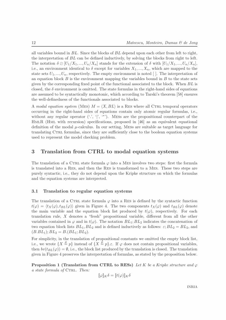
The translation of a Ctrl state formula ϕ into a Res is defined by the syntactic functiont(ϕ) = 〈tX(ϕ), tBL(ϕ)〉 given in Figure 4. The two components tX(ϕ) and tBL(ϕ) denotethe main variable and the equation block list produced by t(ϕ), respectively. For eachtranslation rule, X denotes a “fresh” propositional variable, different from all the othervariables contained in ϕ and in t(ϕ). The notation BL1;BL2 indicates the concatenation oftwo equation block lists BL1, BL2 and is defined inductively as follows: ε;BL2 = BL2, and(B.BL1);BL2 = B.(BL1;BL2).
For simplicity, in the translation of propositional constants we omitted the empty block list,i.e., we wrote {X
µ= p} instead of {X
µ= p}.ε. If ϕ does not contain propositional variables,
then bv(tBL(ϕ)) = ∅, i.e., the block list produced by the translation is closed. The translationgiven in Figure 4 preserves the interpretation of formulas, as stated by the proposition below.
Proposition 1 (Translation from CTRL to RESs) Let K be a Kripke structure and ϕa state formula of Ctrl. Then:
[[ϕ]]Kδ = [[t(ϕ)]]Kδ
INRIA
Computation Tree Regular Logic for Genetic Regulatory Networks 13
for any propositional environment δ.
t(p) = 〈X, {Xµ= p}〉
t(ϕ1 ∨ ϕ2) = 〈X, {Xµ= tX(ϕ1) ∨ tX(ϕ2)}.(tBL(ϕ1); tBL(ϕ2))〉
t(ϕ1 ∧ ϕ2) = 〈X, {Xµ= tX(ϕ1) ∧ tX(ϕ2)}.(tBL(ϕ1); tBL(ϕ2))〉
t(EFρϕ) = 〈X, {Xµ= EFρtX(ϕ)}.tBL(ϕ)〉
t(AFρϕ) = 〈X, {Xµ= AFρtX(ϕ)}.tBL(ϕ)〉
t(EGρϕ) = 〈X, {Xν= EGρtX(ϕ)}.tBL(ϕ)〉
t(AGρϕ) = 〈X, {Xν= AGρtX(ϕ)}.tBL(ϕ)〉
t(EF∞ρ ) = 〈X, {X
ν= EFρX}〉
t(AF∞ρ ) = 〈X, {X
ν= AFρX}〉
t(EG⊣ρ ) = 〈X, {X
µ= EGρX}〉
t(AG⊣ρ ) = 〈X, {X
µ= AGρX}〉
Figure 4: Translation of Ctrl formulas into Ress
To illustrate the translation of Ctrl formulas into Ress, we consider a branching-timeproperty of biological interest, called bistability property [59, 25], which specifies that afteran initial state, two different equilibrium states can be potentially reached. This propertycan be expressed in Ctrl by the following formula:
AGtrue∗.init(EFtrue∗eql1 ∧ EFtrue∗eql2)
where the atomic propositions init , eql1, and eql2 denote the initial state and the two equi-librium states, respectively. By applying the translation defined in Figure 4 to this formula,we obtain the Res below:
〈X, {Xν= AGtrue∗.initY }.{Y
µ= Z1 ∧ Z2}.
{Z1µ= EFtrue∗U1}.{U1
µ= eql1}.{Z2
µ= EFtrue∗U2}.{U2
µ= eql2}.ε〉
The occurrence of the ‘;’ operator produced by the translation of EFtrue∗eql1 ∧ EFtrue∗eql2was expanded in terms of the ‘.’ operator using the definition of ‘;’.
The size (number of variables and operators) of the Res t(ϕ) produced by the translationis linear in the size (number of operators) of the formula ϕ, because every rule given inFigure 4 creates, for each operator present in ϕ, one block containing a single equation withone operator in its right-hand side.
For simplicity, the translation of a state formula ϕ given in Figure 4 does not take care of thestate subformulas ψ that may occur inside the regular formulas ρ. However, these subformu-las must also be translated into Ress in order to be evaluated on a Kripke structureK duringthe model checking procedure. This is done by applying the translation recursively on everysubformula ψ of a regular formula ρ, yielding an additional Res t(ψ) = 〈tX(ψ), tBL(ψ)〉.
RR n° 6521
14 Mateescu, Monteiro, Dumas & de Jong
In practice, the block list tBL(ψ) of each additional Res t(ψ) is concatenated to the blocklist tBL(ϕ) of the Res t(ϕ), and the main variable tX(ψ) replaces the occurrence of thecorresponding subformula ψ, as illustrated by the formula below:
EF(AGtrue∗p)∗q
whose translation yields the following Res:
〈X, {Xµ= EFY ∗Z}.{Z
µ= q}.{Y
ν= AGtrue∗U}.{U
ν= p}.ε〉
However, in order to simplify notations, we can exploit the fact that the Ress produced bytranslating the subformulas ψ are closed, and hence their main variables can be evaluatedindependently from the Res t(ϕ). This allows to safely replace each subformula ψ by a“fresh” atomic proposition pψ, whose interpretation on K is obtained by evaluating the
main variable tX(ψ) of the Res t(ψ). On the example above, the Res becomes 〈X, {Xµ=
EFr∗Z}.{Zµ= q}.ε〉, where r has the same interpretation as the variable Y of the additional
Res 〈Y, {Yν= AGtrue∗U}.{U
ν= p}.ε〉. Therefore, in the sequel we will restrict ourselves to
Ress in which the regular formulas occurring in the right-hand sides of equations are builtonly upon atomic propositions.
3.2 Translation to modal equation systems
Let B = {Xiσ= ϕi}1≤i≤n be an equation block. An equation block {Xn
σ= ψn, Yj
σ= ψj}n<j≤m
is suitable for the substitution of equation Xnσ= ϕn if fv(ψn) ∪
⋃mj=n+1 fv(ψj) = fv(ϕn) and
⋃ni=1 fv(ϕi) ∩ {Yn+1, ..., Ym} = ∅. The notation {Xi
σ= ϕi}1≤i≤n[Xn
σ= ϕn := Xn
σ= ψn, Yj
σ=
ψj}n<j≤m] represents the syntactic substitution of the equation Xnσ= ϕn by the equations
{Xnσ= ψn, Yj
σ= ψj}n<j≤m in B. This definition of substitution, which allows to replace
only the last equation of a block, is general enough: since all equations of a block have thesame fixed point sign, their order does not influence the values of the variables defined inthe block, and therefore any equation of the block can be substituted by bringing it in thelast position.
The translation of the Res equation blocks into Mess is performed by repeatedly applyingvarious transformations on the equation block, most of them being substitutions of equations.
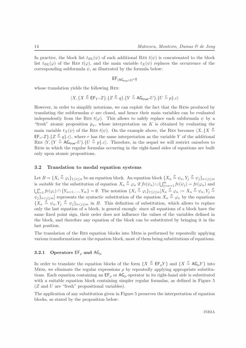
3.2.1 Operators EFρ and AGρ
In order to translate the equation blocks of the form {Xµ= EFρY } and {X
ν= AGρY } into
Mess, we eliminate the regular expressions ρ by repeatedly applying appropriate substitu-tions. Each equation containing an EFρ or AGρ operator in its right-hand side is substitutedwith a suitable equation block containing simpler regular formulas, as defined in Figure 5(Z and U are “fresh” propositional variables).
The application of any substitution given in Figure 5 preserves the interpretation of equationblocks, as stated by the proposition below:
INRIA
Computation Tree Regular Logic for Genetic Regulatory Networks 15
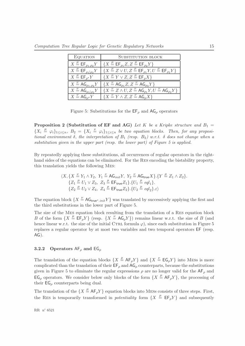
Equation Substitution block
Xµ= EFρ1.ρ2Y {X
µ= EFρ1Z,Z
µ= EFρ2Y }
Xµ= EFρ1|ρ2Y {X
µ= Z ∨ U,Z
µ= EFρ1Y,U
µ= EFρ2Y }
Xµ= EFρ∗Y {X
µ= Y ∨ Z,Z
µ= EFρX}
Xν= AGρ1.ρ2Y {X
ν= AGρ1Z,Z
ν= AGρ2Y }
Xν= AGρ1|ρ2Y {X
ν= Z ∧ U,Z
ν= AGρ1Y,U
ν= AGρ2Y }
Xν= AGρ∗Y {X
ν= Y ∧ Z,Z
ν= AGρX}
Figure 5: Substitutions for the EFρ and AGρ operators
Proposition 2 (Substitution of EF and AG) Let K be a Kripke structure and B1 =
{Xiµ= ϕi}1≤i≤n, B2 = {Xi
ν= ϕi}1≤i≤n be two equation blocks. Then, for any proposi-
tional environment δ, the interpretation of B1 (resp. B2) w.r.t. δ does not change when asubstitution given in the upper part (resp. the lower part) of Figure 5 is applied.
By repeatedly applying these substitutions, all occurrences of regular operators in the right-hand sides of the equations can be eliminated. For the Res encoding the bistability property,this translation yields the following Mes:
〈X, {Xν= Y1 ∧ Y2, Y1
ν= AGinitY, Y2
ν= AGtrueX}.{Y
µ= Z1 ∧ Z2}.
{Z1µ= U1 ∨ Z3, Z3
µ= EFtrueZ1}.{U1
µ= eql1}.
{Z2µ= U2 ∨ Z4, Z4
µ= EFtrueZ2}.{U2
µ= eql2}.ε〉
The equation block {Xν= AGtrue∗.initY } was translated by successively applying the first and
the third substitutions in the lower part of Figure 5.
The size of the Mes equation block resulting from the translation of a Res equation blockB of the form {X
µ= EFρY } (resp. {X
ν= AGρY }) remains linear w.r.t. the size of B (and
hence linear w.r.t. the size of the initial Ctrl formula ϕ), since each substitution in Figure 5replaces a regular operator by at most two variables and two temporal operators EF (resp.AG).
3.2.2 Operators AFρ and EGρ
The translation of the equation blocks {Xµ= AFρY } and {X
ν= EGρY } into Mess is more
complicated than the translation of their EFρ and AGρ counterparts, because the substitutionsgiven in Figure 5 to eliminate the regular expressions ρ are no longer valid for the AFρ and
EGρ operators. We consider below only blocks of the form {Xµ= AFρY }, the processing of
their EGρ counterparts being dual.
The translation of the {Xµ= AFρY } equation blocks into Mess consists of three steps. First,
the Res is temporarily transformed in potentiality form {Xµ= EFρY } and subsequently
RR n° 6521
16 Mateescu, Monteiro, Dumas & de Jong
translated into a potentiality Mes by eliminating the regular expression ρ using the substi-tutions given in Section 3.2.1. Then, the resulting Mes is transformed in guarded form, byeliminating all unguarded (i.e., not preceded by a temporal operator) occurrences of vari-ables in the right-hand sides of equations. Finally, the guarded Mes is determinized, byreplacing all occurrences of EF operators in the right-hand sides of equations by appropriateoccurrences of AF operators in order to retrieve the interpretation of the initial equationblock {X
µ= AFρY }.
We will illustrate each step of the translation on the following example of equation block:
{Xµ= AF(q|p∗)∗.(qr∗).(p∗|q∗)Y }.
Translation to potentiality form
The difficulty of translating an equation block {Xµ= AFρY } into a Mes stems from the
fact that all transition sequences going out of a state have to satisfy ρ before reaching astate satisfying Y , whereas the substitutions in Figure 5 allow to eliminate ρ on individualsequences only. To avoid this difficulty, we switch temporarily to the potentiality form{X
µ= EFρY }, we eliminate ρ by applying the substitutions, and we continue working with
the resulting potentiality Mes, which characterizes the existence of individual sequencessatisfying ρ. The size of this Mes is linear w.r.t. the size of the initial block {X
µ= AFρY },
as stated in Section 3.2.1. Figure 6 shows the potentiality Mes obtained from the equationblock considered above by switching to potentiality form and applying the substitutions inFigure 5 (all equations have the sign µ, which was omitted for simplicity).
X = EF(q|p∗)∗Z1 X = Z3 ∨ Z1 X = Z3 ∨ Z1
Z3 = EFq|p∗X Z3 = Z4 ∨ Z5 Z3 = Z4 ∨ Z5
Z5 = EFqX Z5 = EFqXZ4 = EFp∗X Z4 = Z6 ∨X Z4 = Z6 ∨X
Z6 = EFpZ4 Z6 = EFpZ4
Z1 = EFqr∗Z2 Z1 = EFqZ7 Z1 = EFqZ7
Z7 = EFr∗Z2 Z7 = Z8 ∨ Z2 Z7 = Z8 ∨ Z2
Z8 = EFrZ7 Z8 = EFrZ7
Z2 = EFp∗|q∗Y Z2 = Z9 ∨ Z10 Z2 = Z9 ∨ Z10
Z9 = EFp∗Y Z9 = Z11 ∨ Y Z9 = Z11 ∨ YZ11 = EFpZ9 Z11 = EFpZ9
Z10 = EFq∗Y Z10 = Z12 ∨ Y Z10 = Z12 ∨ YZ12 = EFqZ10 Z12 = EFqZ10
Figure 6: Translation of {Xµ= AF(q|p∗)∗.(qr∗).(p∗|q∗)Y } to a potentiality Mes
The right-hand sides of the equations of the potentiality Mes may contain unguarded oc-currences of propositional variables (i.e., not preceded by any EF operator), such as variable
INRIA
Computation Tree Regular Logic for Genetic Regulatory Networks 17
Z1 in the equation X = Z3 ∨ Z1. These occurrences will be eliminated in the next step ofthe translation.
Translation to guarded form
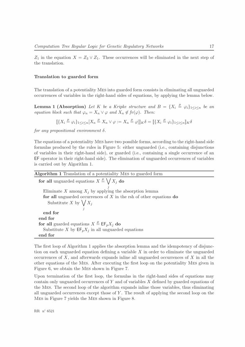
The translation of a potentiality Mes into guarded form consists in eliminating all unguardedoccurrences of variables in the right-hand sides of equations, by applying the lemma below.
Lemma 1 (Absorption) Let K be a Kripke structure and B = {Xiµ= ϕi}1≤i≤n be an
equation block such that ϕn = Xn ∨ ϕ and Xn 6∈ fv(ϕ). Then:
[[{Xiµ= ϕi}1≤i≤n[Xn
µ= Xn ∨ ϕ := Xn
µ= ϕ]]]Kδ = [[{Xi
µ= ϕi}1≤i≤n]]Kδ
for any propositional environment δ.
The equations of a potentiality Mes have two possible forms, according to the right-hand sideformulas produced by the rules in Figure 5: either unguarded (i.e., containing disjunctionsof variables in their right-hand side), or guarded (i.e., containing a single occurrence of anEF operator in their right-hand side). The elimination of unguarded occurrences of variablesis carried out by Algorithm 1.
Algorithm 1 Translation of a potentiality Mes to guarded form
for all unguarded equations Xµ=∨
j
Xj do
Eliminate X among Xj by applying the absorption lemmafor all unguarded occurrences of X in the rsh of other equations do
Substitute X by∨
j
Xj
end forend forfor all guarded equations X
µ= EFpXj do
Substitute X by EFpXj in all unguarded equationsend for
The first loop of Algorithm 1 applies the absorption lemma and the idempotency of disjunc-tion on each unguarded equation defining a variable X in order to eliminate the unguardedoccurrences of X, and afterwards expands inline all unguarded occurrences of X in all theother equations of the Mes. After executing the first loop on the potentiality Mes given inFigure 6, we obtain the Mes shown in Figure 7.
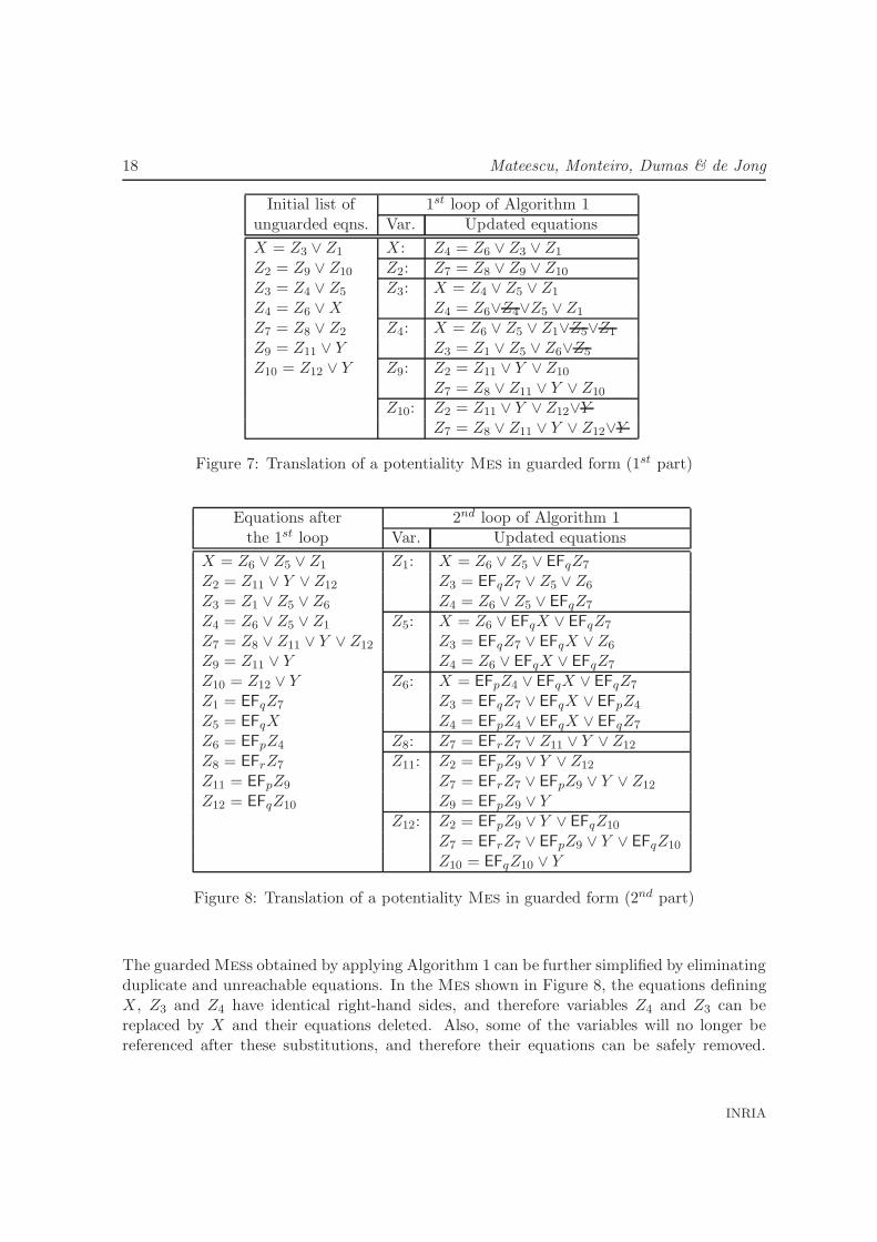
Upon termination of the first loop, the formulas in the right-hand sides of equations maycontain only unguarded occurrences of Y and of variables X defined by guarded equations ofthe Mes. The second loop of the algorithm expands inline those variables, thus eliminatingall unguarded occurrences except those of Y . The result of applying the second loop on theMes in Figure 7 yields the Mes shown in Figure 8.
RR n° 6521
18 Mateescu, Monteiro, Dumas & de Jong
Initial list of 1st loop of Algorithm 1unguarded eqns. Var. Updated equations
X = Z3 ∨ Z1 X: Z4 = Z6 ∨ Z3 ∨ Z1
Z2 = Z9 ∨ Z10 Z2: Z7 = Z8 ∨ Z9 ∨ Z10
Z3 = Z4 ∨ Z5 Z3: X = Z4 ∨ Z5 ∨ Z1
Z4 = Z6 ∨X Z4 = Z6∨Z4∨Z5 ∨ Z1
Z7 = Z8 ∨ Z2 Z4: X = Z6 ∨ Z5 ∨ Z1∨Z5∨Z1
Z9 = Z11 ∨ Y Z3 = Z1 ∨ Z5 ∨ Z6∨Z5
Z10 = Z12 ∨ Y Z9: Z2 = Z11 ∨ Y ∨ Z10
Z7 = Z8 ∨ Z11 ∨ Y ∨ Z10
Z10: Z2 = Z11 ∨ Y ∨ Z12∨YZ7 = Z8 ∨ Z11 ∨ Y ∨ Z12∨Y
Figure 7: Translation of a potentiality Mes in guarded form (1st part)
Equations after 2nd loop of Algorithm 1the 1st loop Var. Updated equations
X = Z6 ∨ Z5 ∨ Z1 Z1: X = Z6 ∨ Z5 ∨ EFqZ7
Z2 = Z11 ∨ Y ∨ Z12 Z3 = EFqZ7 ∨ Z5 ∨ Z6
Z3 = Z1 ∨ Z5 ∨ Z6 Z4 = Z6 ∨ Z5 ∨ EFqZ7
Z4 = Z6 ∨ Z5 ∨ Z1 Z5: X = Z6 ∨ EFqX ∨ EFqZ7
Z7 = Z8 ∨ Z11 ∨ Y ∨ Z12 Z3 = EFqZ7 ∨ EFqX ∨ Z6
Z9 = Z11 ∨ Y Z4 = Z6 ∨ EFqX ∨ EFqZ7
Z10 = Z12 ∨ Y Z6: X = EFpZ4 ∨ EFqX ∨ EFqZ7
Z1 = EFqZ7 Z3 = EFqZ7 ∨ EFqX ∨ EFpZ4
Z5 = EFqX Z4 = EFpZ4 ∨ EFqX ∨ EFqZ7
Z6 = EFpZ4 Z8: Z7 = EFrZ7 ∨ Z11 ∨ Y ∨ Z12
Z8 = EFrZ7 Z11: Z2 = EFpZ9 ∨ Y ∨ Z12
Z11 = EFpZ9 Z7 = EFrZ7 ∨ EFpZ9 ∨ Y ∨ Z12
Z12 = EFqZ10 Z9 = EFpZ9 ∨ YZ12: Z2 = EFpZ9 ∨ Y ∨ EFqZ10
Z7 = EFrZ7 ∨ EFpZ9 ∨ Y ∨ EFqZ10
Z10 = EFqZ10 ∨ Y
Figure 8: Translation of a potentiality Mes in guarded form (2nd part)
The guarded Mess obtained by applying Algorithm 1 can be further simplified by eliminatingduplicate and unreachable equations. In the Mes shown in Figure 8, the equations definingX, Z3 and Z4 have identical right-hand sides, and therefore variables Z4 and Z3 can bereplaced by X and their equations deleted. Also, some of the variables will no longer bereferenced after these substitutions, and therefore their equations can be safely removed.
INRIA
Computation Tree Regular Logic for Genetic Regulatory Networks 19
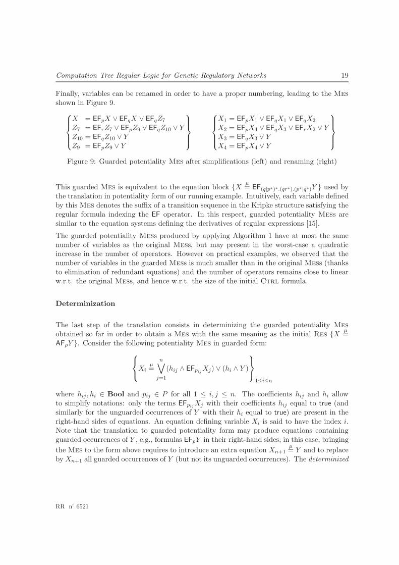
Finally, variables can be renamed in order to have a proper numbering, leading to the Messhown in Figure 9.
X = EFpX ∨ EFqX ∨ EFqZ7
Z7 = EFrZ7 ∨ EFpZ9 ∨ EFqZ10 ∨ YZ10 = EFqZ10 ∨ YZ9 = EFpZ9 ∨ Y
X1 = EFpX1 ∨ EFqX1 ∨ EFqX2
X2 = EFpX4 ∨ EFqX3 ∨ EFrX2 ∨ YX3 = EFqX3 ∨ YX4 = EFpX4 ∨ Y
Figure 9: Guarded potentiality Mes after simplifications (left) and renaming (right)
This guarded Mes is equivalent to the equation block {Xµ= EF(q|p∗)∗.(qr∗).(p∗|q∗)Y } used by
the translation in potentiality form of our running example. Intuitively, each variable definedby this Mes denotes the suffix of a transition sequence in the Kripke structure satisfying theregular formula indexing the EF operator. In this respect, guarded potentiality Mess aresimilar to the equation systems defining the derivatives of regular expressions [15].
The guarded potentiality Mess produced by applying Algorithm 1 have at most the samenumber of variables as the original Mess, but may present in the worst-case a quadraticincrease in the number of operators. However on practical examples, we observed that thenumber of variables in the guarded Mess is much smaller than in the original Mess (thanksto elimination of redundant equations) and the number of operators remains close to linearw.r.t. the original Mess, and hence w.r.t. the size of the initial Ctrl formula.
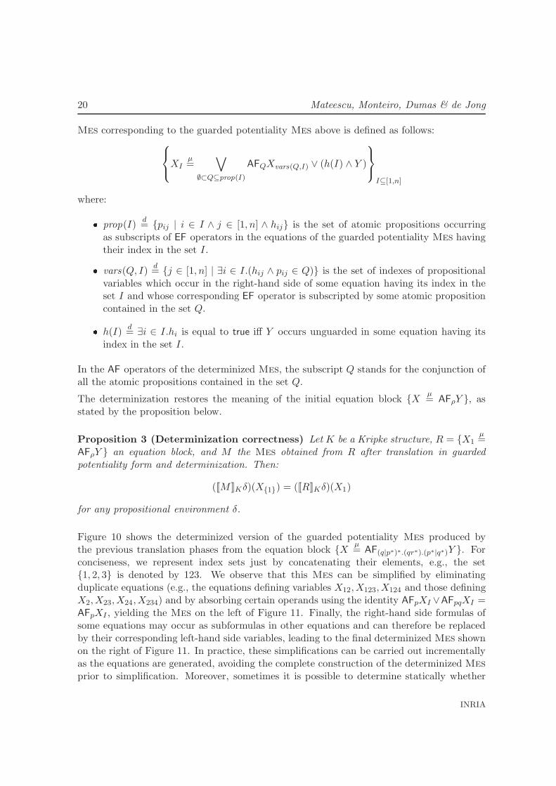
Determinization
The last step of the translation consists in determinizing the guarded potentiality Mesobtained so far in order to obtain a Mes with the same meaning as the initial Res {X
µ=
AFρY }. Consider the following potentiality Mes in guarded form:
Xiµ=
n∨
j=1
(hij ∧ EFpijXj) ∨ (hi ∧ Y )
1≤i≤n
where hij , hi ∈ Bool and pij ∈ P for all 1 ≤ i, j ≤ n. The coefficients hij and hi allowto simplify notations: only the terms EFpij
Xj with their coefficients hij equal to true (andsimilarly for the unguarded occurrences of Y with their hi equal to true) are present in theright-hand sides of equations. An equation defining variable Xi is said to have the index i.Note that the translation to guarded potentiality form may produce equations containingguarded occurrences of Y , e.g., formulas EFpY in their right-hand sides; in this case, bringing
the Mes to the form above requires to introduce an extra equation Xn+1µ= Y and to replace
by Xn+1 all guarded occurrences of Y (but not its unguarded occurrences). The determinized
RR n° 6521
20 Mateescu, Monteiro, Dumas & de Jong
Mes corresponding to the guarded potentiality Mes above is defined as follows:
XIµ=
∨
∅⊂Q⊆prop(I)
AFQXvars(Q,I) ∨ (h(I) ∧ Y )
I⊆[1,n]
where:� prop(I)d= {pij | i ∈ I ∧ j ∈ [1, n] ∧ hij} is the set of atomic propositions occurring
as subscripts of EF operators in the equations of the guarded potentiality Mes havingtheir index in the set I.� vars(Q, I)
d= {j ∈ [1, n] | ∃i ∈ I.(hij ∧ pij ∈ Q)} is the set of indexes of propositional
variables which occur in the right-hand side of some equation having its index in theset I and whose corresponding EF operator is subscripted by some atomic propositioncontained in the set Q.� h(I)
d= ∃i ∈ I.hi is equal to true iff Y occurs unguarded in some equation having its
index in the set I.
In the AF operators of the determinized Mes, the subscript Q stands for the conjunction ofall the atomic propositions contained in the set Q.
The determinization restores the meaning of the initial equation block {Xµ= AFρY }, as
stated by the proposition below.
Proposition 3 (Determinization correctness) Let K be a Kripke structure, R = {X1µ=
AFρY } an equation block, and M the Mes obtained from R after translation in guardedpotentiality form and determinization. Then:
([[M ]]Kδ)(X{1}) = ([[R]]Kδ)(X1)
for any propositional environment δ.
Figure 10 shows the determinized version of the guarded potentiality Mes produced bythe previous translation phases from the equation block {X
µ= AF(q|p∗)∗.(qr∗).(p∗|q∗)Y }. For
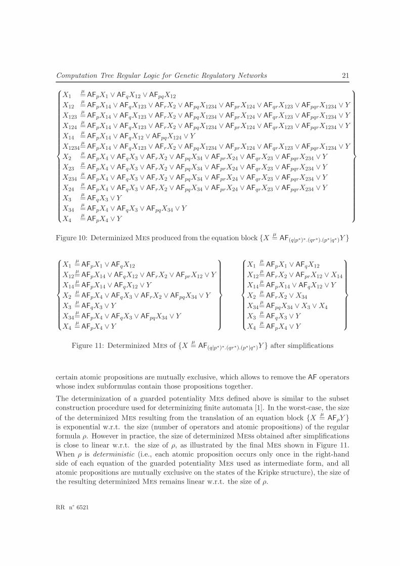
conciseness, we represent index sets just by concatenating their elements, e.g., the set{1, 2, 3} is denoted by 123. We observe that this Mes can be simplified by eliminatingduplicate equations (e.g., the equations defining variables X12,X123,X124 and those definingX2,X23,X24,X234) and by absorbing certain operands using the identity AFpXI ∨AFpqXI =AFpXI , yielding the Mes on the left of Figure 11. Finally, the right-hand side formulas ofsome equations may occur as subformulas in other equations and can therefore be replacedby their corresponding left-hand side variables, leading to the final determinized Mes shownon the right of Figure 11. In practice, these simplifications can be carried out incrementallyas the equations are generated, avoiding the complete construction of the determinized Mesprior to simplification. Moreover, sometimes it is possible to determine statically whether
INRIA
Computation Tree Regular Logic for Genetic Regulatory Networks 21
X1µ= AFpX1 ∨ AFqX12 ∨ AFpqX12
X12µ= AFpX14 ∨ AFqX123 ∨ AFrX2 ∨ AFpqX1234 ∨ AFprX124 ∨ AFqrX123 ∨ AFpqrX1234 ∨ Y
X123µ= AFpX14 ∨ AFqX123 ∨ AFrX2 ∨ AFpqX1234 ∨ AFprX124 ∨ AFqrX123 ∨ AFpqrX1234 ∨ Y
X124µ= AFpX14 ∨ AFqX123 ∨ AFrX2 ∨ AFpqX1234 ∨ AFprX124 ∨ AFqrX123 ∨ AFpqrX1234 ∨ Y
X14µ= AFpX14 ∨ AFqX12 ∨ AFpqX124 ∨ Y
X1234µ= AFpX14 ∨ AFqX123 ∨ AFrX2 ∨ AFpqX1234 ∨ AFprX124 ∨ AFqrX123 ∨ AFpqrX1234 ∨ Y
X2µ= AFpX4 ∨ AFqX3 ∨ AFrX2 ∨ AFpqX34 ∨ AFprX24 ∨ AFqrX23 ∨ AFpqrX234 ∨ Y
X23µ= AFpX4 ∨ AFqX3 ∨ AFrX2 ∨ AFpqX34 ∨ AFprX24 ∨ AFqrX23 ∨ AFpqrX234 ∨ Y
X234µ= AFpX4 ∨ AFqX3 ∨ AFrX2 ∨ AFpqX34 ∨ AFprX24 ∨ AFqrX23 ∨ AFpqrX234 ∨ Y
X24µ= AFpX4 ∨ AFqX3 ∨ AFrX2 ∨ AFpqX34 ∨ AFprX24 ∨ AFqrX23 ∨ AFpqrX234 ∨ Y
X3µ= AFqX3 ∨ Y
X34µ= AFpX4 ∨ AFqX3 ∨ AFpqX34 ∨ Y
X4µ= AFpX4 ∨ Y
Figure 10: Determinized Mes produced from the equation block {Xµ= AF(q|p∗)∗.(qr∗).(p∗|q∗)Y }
X1µ= AFpX1 ∨ AFqX12
X12µ= AFpX14 ∨ AFqX12 ∨ AFrX2 ∨ AFprX12 ∨ Y
X14µ= AFpX14 ∨ AFqX12 ∨ Y
X2µ= AFpX4 ∨ AFqX3 ∨ AFrX2 ∨ AFpqX34 ∨ Y
X3µ= AFqX3 ∨ Y
X34µ= AFpX4 ∨ AFqX3 ∨ AFpqX34 ∨ Y
X4µ= AFpX4 ∨ Y
X1µ= AFpX1 ∨ AFqX12
X12µ= AFrX2 ∨ AFprX12 ∨X14
X14µ= AFpX14 ∨ AFqX12 ∨ Y
X2µ= AFrX2 ∨X34
X34µ= AFpqX34 ∨X3 ∨X4
X3µ= AFqX3 ∨ Y
X4µ= AFpX4 ∨ Y
Figure 11: Determinized Mes of {Xµ= AF(q|p∗)∗.(qr∗).(p∗|q∗)Y } after simplifications
certain atomic propositions are mutually exclusive, which allows to remove the AF operatorswhose index subformulas contain those propositions together.
The determinization of a guarded potentiality Mes defined above is similar to the subsetconstruction procedure used for determinizing finite automata [1]. In the worst-case, the size
of the determinized Mes resulting from the translation of an equation block {Xµ= AFρY }
is exponential w.r.t. the size (number of operators and atomic propositions) of the regularformula ρ. However in practice, the size of determinized Mess obtained after simplificationsis close to linear w.r.t. the size of ρ, as illustrated by the final Mes shown in Figure 11.When ρ is deterministic (i.e., each atomic proposition occurs only once in the right-handside of each equation of the guarded potentiality Mes used as intermediate form, and allatomic propositions are mutually exclusive on the states of the Kripke structure), the size ofthe resulting determinized Mes remains linear w.r.t. the size of ρ.
RR n° 6521
22 Mateescu, Monteiro, Dumas & de Jong
3.2.3 Operators EF∞ρ , AF∞
ρ , EG⊣ρ , and AG⊣
ρ
According to the rules given in Fig 4, the EF∞ρ and AF∞
ρ operators are translated into equation
blocks of the form {Xν= EFρX} and {X
ν= AFρX}, respectively. The interpretation of these
equation blocks is given by νΦe and νΦa, where the functionals Φe,Φa : 2S → 2S are definedas follows:
Φe(U) = [[EFρX]]K [U/X] = ([[{X1µ= EFρX}]]K [U/X])(X1)
Φa(U) = [[AFρX]]K [U/X] = ([[{X1µ= AFρX}]]K [U/X])(X1).
The evaluation of the EF∞ρ and AF∞
ρ operators requires to compute the maximal fixed pointsof the functionals Φe and Φa, which are defined in turn as the minimal fixed points of thefunctionals associated to the Ress Re = {X1
µ= EFρX} and Ra = {X1
µ= AFρX}. Therefore,
these operators belong to Lµ2, the µ-calculus fragment of alternation depth 2 [27], whichallows one level of mutual recursion between minimal and maximal fixed points1. Thecomplexity of checking Lµ2 formulas on a Kripke structure K is in general quadratic inthe size of K; however, we can exploit the particular structure of Re and Ra in order todevise linear-time on-the-fly model checking algorithms for the EF∞
ρ operator and (when ρis deterministic) for the AF∞
ρ operator, as shown in Section 4.
The operators EG⊣ρ and AG⊣
ρ are handled dually w.r.t. AF∞ρ and EF∞
ρ , respectively.
4 On-the-fly model checking
Given a Kripke structure K = 〈S,P,L, T, s0〉 and a Ctrl state formula ϕ, the on-the-flymodel checking problem consists in determining whether the initial state s0 of K satisfiesϕ by exploring the transition relation T in a forward manner starting at s0. Our objectiveis to reuse the on-the-fly model checking technology already available in the setting of theMcl property specification language [52, 51], an extension of Lµ1 with various constructs,among which the regular expressions and fairness operators of Pdl-∆. Mcl is interpretedon labeled transition systems (Ltss) modeling the behaviour of concurrent programs writ-ten in action-based specification languages, such as process algebras. The model checkingprocedure of Mcl relies upon a translation to the alternation-free fragment of HmlR, whichis an equivalent equational representation of Lµ1. The on-the-fly model checking problemof a HmlR specification on an Lts is subsequently rephrased as the local resolution of analternation-free boolean equation system (Bes), which is carried out using specialized linear-time algorithms [50]. Therefore, in order to reuse this technology it is necessary to switchfrom Kripke structures to Ltss and to translate Ctrl formulas into HmlR specifications.
Kripke structures are converted into Ltss in the classical way [21], i.e., for each state s, theatomic propositions holding at s in the Kripke structure are migrated to the actions labelingthe transitions going out of s in the Lts. Formally, the Lts corresponding to a Kripke
1The EF∞
ρ and AF∞
ρ operators belong strictly to Lµ2 only when ρ contains iteration operators; otherwise,they belong to Lµ1, the µ-calculus fragment of alternation depth 1, which has a linear-time model checkingcomplexity [22].
INRIA
Computation Tree Regular Logic for Genetic Regulatory Networks 23
structure is defined as 〈S, 2P , {(s1, L(s1), s2) ∈ S × 2P × S | s1 →T s2}, s0〉, where 2P is theset of actions (sets of atomic propositions). This translation is succinct, i.e., every state andtransition of the Kripke structure is mapped to a state and a transition of the Lts. It is alsosuitable for on-the-fly verification because it can be carried out during a forward traversalof the transition relation. As regards the translation of Ctrl state formulas to HmlR, webriefly explain below how this is done for each temporal operator.
4.1 Operators EFρ, AFρ, EGρ, and AGρ
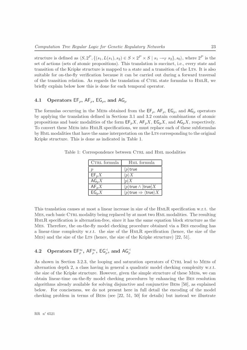
The formulas occurring in the Mess obtained from the EFρ, AFρ, EGρ, and AGρ operatorsby applying the translation defined in Sections 3.1 and 3.2 contain combinations of atomicpropositions and basic modalities of the form EFpX, AFpX, EGpX, and AGpX, respectively.To convert these Mess into HmlR specifications, we must replace each of these subformulasby Hml modalities that have the same interpretation on the Lts corresponding to the originalKripke structure. This is done as indicated in Table 1.
Table 1: Correspondence between Ctrl and Hml modalities
Ctrl formula Hml formula
p 〈p〉true
EFpX 〈p〉X
AGpX [p]X
AFpX 〈p〉true ∧ [true]X
EGpX 〈p〉true ⇒ 〈true〉X
This translation causes at most a linear increase in size of the HmlR specification w.r.t. theMes, each basic Ctrl modality being replaced by at most two Hml modalities. The resultingHmlR specification is alternation-free, since it has the same equation block structure as theMes. Therefore, the on-the-fly model checking procedure obtained via a Bes encoding hasa linear-time complexity w.r.t. the size of the HmlR specification (hence, the size of theMes) and the size of the Lts (hence, the size of the Kripke structure) [22, 51].
4.2 Operators EF∞ρ , AF∞
ρ , EG⊣ρ , and AG⊣
ρ
As shown in Section 3.2.3, the looping and saturation operators of Ctrl lead to Mess ofalternation depth 2, a class having in general a quadratic model checking complexity w.r.t.the size of the Kripke structure. However, given the simple structure of these Mess, we canobtain linear-time on-the-fly model checking procedures by enhancing the Bes resolutionalgorithms already available for solving disjunctive and conjunctive Bess [50], as explainedbelow. For conciseness, we do not present here in full detail the encoding of the modelchecking problem in terms of Bess (see [22, 51, 50] for details) but instead we illustrate
RR n° 6521
24 Mateescu, Monteiro, Dumas & de Jong
it on examples. We consider only the looping operators EF∞ρ and the AF∞
ρ operators, the
saturation operators AG⊣ρ and EG⊣
ρ being handled dually.
4.2.1 Operator EF∞ρ
The EF∞ρ operator yields a Res of the form {X
ν= EFρX}. To evaluate this Res on a Kripke
structure (or equivalently, the corresponding HmlR specification on the Lts derived fromthe Kripke structure), we abusively switch its sign to µ and take care to preserve its originalmeaning during the resolution of the Bes encoding the model checking problem. The Mesobtained after applying the translation given in Section 3.2.1 contains only disjunctions andEF operators, which yield diamond modalities in the HmlR specification. Therefore, the Besencoding the model checking problem is disjunctive, and could be solved using the algorithmA4 proposed in [50].
If the EF∞ρ formula is false, the solution of the {X
µ= EFρX} is also false, since by switching
the sign from ν to µ we obtain an equation block with a “smaller” interpretation. If EF∞ρ is
true, the Kripke structure contains an infinite sequence made of subsequences satisfying ρ,which must end with a cycle because the set of states is finite. The model checking algorithmmust therefore detect the presence of such cycles and record that all the states occurring onthem satisfy EF∞
ρ . This cycle detection can be performed by the A4cyc algorithm proposedin [52], which is an extended version of the A4 algorithm dedicated to disjunctive Bess.
Formula:
p q
q
10 2 3
4
X22
Ks:
Mes:
EF∞true∗.p.true∗.q
X0µ= X1
X1µ= EFpX2 ∨ EFtrueX1
X2µ= EFqX0 ∨ EFtrueX2
Bes: Xij = sj |= Xi X00
X10
X11
X24X23
X01 X21
X04
X13
X12
X14
Figure 12: Evaluation of a EF∞ formula using the A4cyc algorithm
Figure 12 illustrates the execution of A4cyc for checking a EF∞ρ formula on a Kripke structure.
For simplicity, we show the verification by considering directly the Res and the Kripkestructure instead of the corresponding HmlR specification and Lts. The verification problemis reformulated as the resolution of a Bes in which a variable Xij is true iff the state si of theKripke structure satisfies the propositional variable Xj of the Res. The Bes is represented
INRIA
Computation Tree Regular Logic for Genetic Regulatory Networks 25
by means of its associated boolean graph [2], which gives a more intuitive representation of thedependencies between boolean variables. The variable X0 of the Res was defined initially bythe equationX0
µ= EFρX0 and therefore it plays a special role: every sequence of dependencies
in the boolean graph relating two variables X0j denotes a sequence of transitions matchingρ in the Kripke structure. Algorithm A4cyc marks all variables X0j and searches for cyclescontaining a marked variable: if such a cycle exists, then an infinite sequence satisfying ρexists in the Kripke structure and the formula is true. In the example shown on Figure 12,the boolean graph associated to the disjunctive Bes contains a cycle (surrounded by thedashed line) going through the marked variable X01, meaning that the property holds onthe Kripke structure.
The A4cyc algorithm has a linear time complexity w.r.t. the size of the boolean graph [52],which makes the complexity of evaluating an EF∞
ρ formula linear w.r.t. the size of ρ and ofthe Kripke structure.
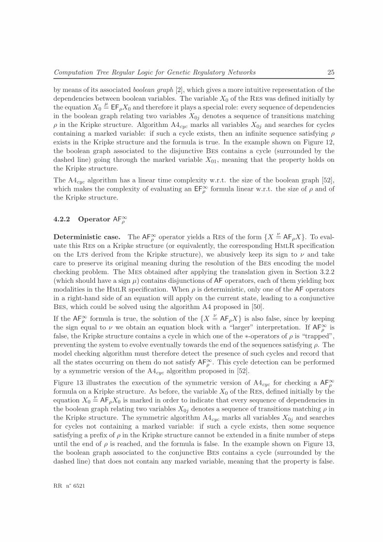
4.2.2 Operator AF∞ρ
Deterministic case. The AF∞ρ operator yields a Res of the form {X
ν= AFρX}. To eval-
uate this Res on a Kripke structure (or equivalently, the corresponding HmlR specificationon the Lts derived from the Kripke structure), we abusively keep its sign to ν and takecare to preserve its original meaning during the resolution of the Bes encoding the modelchecking problem. The Mes obtained after applying the translation given in Section 3.2.2(which should have a sign µ) contains disjunctions of AF operators, each of them yielding boxmodalities in the HmlR specification. When ρ is deterministic, only one of the AF operatorsin a right-hand side of an equation will apply on the current state, leading to a conjunctiveBes, which could be solved using the algorithm A4 proposed in [50].
If the AF∞ρ formula is true, the solution of the {X
ν= AFρX} is also false, since by keeping
the sign equal to ν we obtain an equation block with a “larger” interpretation. If AF∞ρ is
false, the Kripke structure contains a cycle in which one of the ∗-operators of ρ is “trapped”,preventing the system to evolve eventually towards the end of the sequences satisfying ρ. Themodel checking algorithm must therefore detect the presence of such cycles and record thatall the states occurring on them do not satisfy AF∞
ρ . This cycle detection can be performedby a symmetric version of the A4cyc algorithm proposed in [52].
Figure 13 illustrates the execution of the symmetric version of A4cyc for checking a AF∞ρ
formula on a Kripke structure. As before, the variable X0 of the Res, defined initially by theequation X0
ν= AFρX0 is marked in order to indicate that every sequence of dependencies in
the boolean graph relating two variables X0j denotes a sequence of transitions matching ρ inthe Kripke structure. The symmetric algorithm A4cyc marks all variables X0j and searchesfor cycles not containing a marked variable: if such a cycle exists, then some sequencesatisfying a prefix of ρ in the Kripke structure cannot be extended in a finite number of stepsuntil the end of ρ is reached, and the formula is false. In the example shown on Figure 13,the boolean graph associated to the conjunctive Bes contains a cycle (surrounded by thedashed line) that does not contain any marked variable, meaning that the property is false.
RR n° 6521
26 Mateescu, Monteiro, Dumas & de Jong
Formula:
p r
r
10 2 3
4
p q
X00
X10
X11
X12 X14
X13 X01
Ks:
Mes:
AF∞(p|q)∗.r
{
X0ν= X1
X1ν= AFpX1 ∨ AFqX1 ∨ AFrX0
}
Bes: Xij = sj |= Xi
Figure 13: Evaluation of a AF∞ deterministic formula using the symmetric A4cyc algorithm
The symmetric A4cyc algorithm has a linear time complexity w.r.t. the size of the booleangraph [52], which makes the complexity of evaluating a deterministic AF∞
ρ formula linearw.r.t. the size of ρ and of the Kripke structure.
Nondeterministic case. When ρ is nondeterministic, the Bes resulting from the transla-tion above has a general shape, i.e., the right-hand sides of its equations contain both ∨ and∧ connectors. In this case, one can apply the on-the-fly resolution algorithms dedicated toBess of alternation depth 2 [61]. These algorithms have a worst-case comlexity quadratic inthe size of the Bes, which yields a quadratic complexity w.r.t. the size of the Mes producedby translating AFρX and the size of the Kripke structure.
4.3 Complexity
The complexity of the model checking procedure presented in Sections 3, 4.1, and 4.2 issummarized in Table 2. The EFρ and EF∞
ρ operators, together with their respective duals
AGρ and AG⊣ρ , are evaluated in linear-time w.r.t. the size of the formula and the size of
the Kripke structure. Moreover, the evaluation of these operators has a memory complexityO(|ρ| · |S|), meaning that only the states (and not the transitions) of the Kripke structure arestored; this is a consequence of using the memory-efficient Bes resolution algorithms A4 [50]and A4cyc [52] dedicated to disjunctive and conjunctive Bess. This fragment of Ctrl is thestate-based counterpart of Pdl-∆ [57], which is more expressive than Ctl∗ [26]. Of course,this does not yield a linear-time model checking procedure for Ctl∗ (nor for its fragmentLtl), because the translation from Ctl∗ to Pdl-∆ is not succinct [62]. The advantage of thelinear-time model checking procedure for the EF∞
ρ potential looping operator (obtained dueto the Bes resolution algorithm A4cyc [52]) is to allow an efficient detection of complex cyclesin the Kripke structure, which describe oscillation properties [17]. The EF∞
ρ operator is also
INRIA
Computation Tree Regular Logic for Genetic Regulatory Networks 27
useful for characterizing fairness properties in concurrent systems, such as the existence ofcomplex unfair executions in resource locking protocols [5].
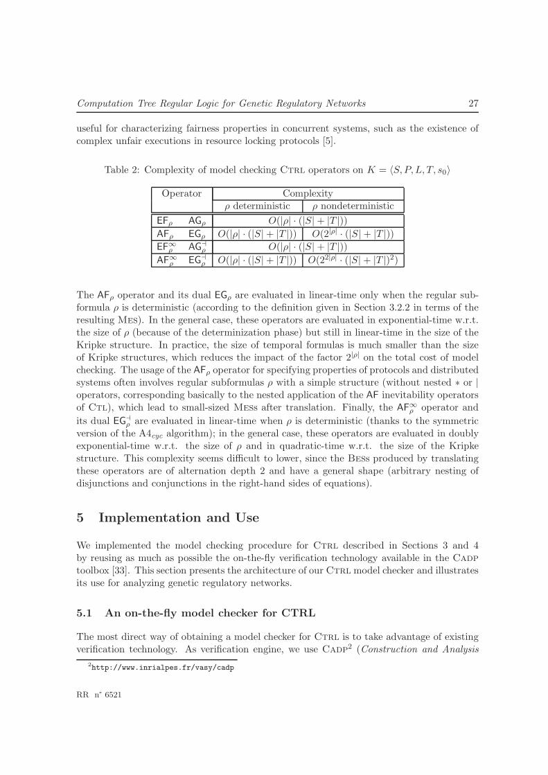
Table 2: Complexity of model checking Ctrl operators on K = 〈S,P,L, T, s0〉
Operator Complexityρ deterministic ρ nondeterministic
EFρ AGρ O(|ρ| · (|S| + |T |))
AFρ EGρ O(|ρ| · (|S| + |T |)) O(2|ρ| · (|S| + |T |))EF∞
ρ AG⊣ρ O(|ρ| · (|S| + |T |))
AF∞ρ EG⊣
ρ O(|ρ| · (|S| + |T |)) O(22|ρ| · (|S| + |T |)2)
The AFρ operator and its dual EGρ are evaluated in linear-time only when the regular sub-formula ρ is deterministic (according to the definition given in Section 3.2.2 in terms of theresulting Mes). In the general case, these operators are evaluated in exponential-time w.r.t.the size of ρ (because of the determinization phase) but still in linear-time in the size of theKripke structure. In practice, the size of temporal formulas is much smaller than the sizeof Kripke structures, which reduces the impact of the factor 2|ρ| on the total cost of modelchecking. The usage of the AFρ operator for specifying properties of protocols and distributedsystems often involves regular subformulas ρ with a simple structure (without nested ∗ or |operators, corresponding basically to the nested application of the AF inevitability operatorsof Ctl), which lead to small-sized Mess after translation. Finally, the AF∞
ρ operator and
its dual EG⊣ρ are evaluated in linear-time when ρ is deterministic (thanks to the symmetric
version of the A4cyc algorithm); in the general case, these operators are evaluated in doublyexponential-time w.r.t. the size of ρ and in quadratic-time w.r.t. the size of the Kripkestructure. This complexity seems difficult to lower, since the Bess produced by translatingthese operators are of alternation depth 2 and have a general shape (arbitrary nesting ofdisjunctions and conjunctions in the right-hand sides of equations).
5 Implementation and Use
We implemented the model checking procedure for Ctrl described in Sections 3 and 4by reusing as much as possible the on-the-fly verification technology available in the Cadptoolbox [33]. This section presents the architecture of our Ctrl model checker and illustratesits use for analyzing genetic regulatory networks.
5.1 An on-the-fly model checker for CTRL
The most direct way of obtaining a model checker for Ctrl is to take advantage of existingverification technology. As verification engine, we use Cadp2 (Construction and Analysis
2http://www.inrialpes.fr/vasy/cadp
RR n° 6521
28 Mateescu, Monteiro, Dumas & de Jong
of Distributed Processes) [33], a state-of-the-art verification toolbox for concurrent asyn-chronous systems. Cadp offers a wide range of functionalities assisting the user throughoutthe design process: compilation and rapid prototyping, random execution, interactive andguided simulation, model checking and equivalence checking, test generation, and perfor-mance evaluation. The toolbox accepts as input process algebraic descriptions in Lotos [39]or Chp [49], as well as networks of communicating automata in the Exp language [45].
The tools of Cadp operate on labeled transition systems (Ltss), which are represented eitherexplicitly (by their list of transitions) as compact binary files encoded in the Bcg (BinaryCoded Graphs) format, or implicitly (by their successor function) as C programs compli-ant with the Open/Cæsar interface [31]. Cadp contains the on-the-fly model checkerEvaluator [51], which evaluates regular alternation-free µ-calculus (Lµreg
1 ) formulas onimplicit Ltss. The tool works by translating the verification problem in terms of the localresolution of a Bes, which is done using the algorithms available in the generic Cæsar Solvelibrary [50]. Evaluator 3.6 uses HmlR as intermediate language: Lµreg
1 formulas aretranslated into HmlR specifications, whose evaluation on implicit Ltss can be straightfor-wardly encoded as a local Bes resolution. The tool generates full diagnostics (examplesand counterexamples) illustrating the truth value of the formulas, and is also equipped withmacro-definition mechanisms allowing the creation of reusable libraries of derived temporaloperators.
(.aut.bcg.c)
(.aut .bcg)
(.ctrl)
(.blk)
(.mcl)
ρex
pan
sion
Abusi
veρ
expan
sion
Tra
nsl
atio
n
Tra
nsl
atio
ngu
arded
form
Det
erm
iniz
atio
n
On-the-flyresolution
Res Mes
Mes Mes Mes
Lµreg1
HmlR
Bes
answer
Lts
Lts
Res
Ctrl
EFρ/AGρ
AFρ/EGρ
Ctrl translation
Cadp Evaluator
Expan
sion
Figure 14: Ctrl translator and its connection to the Evaluator model checker of Cadp
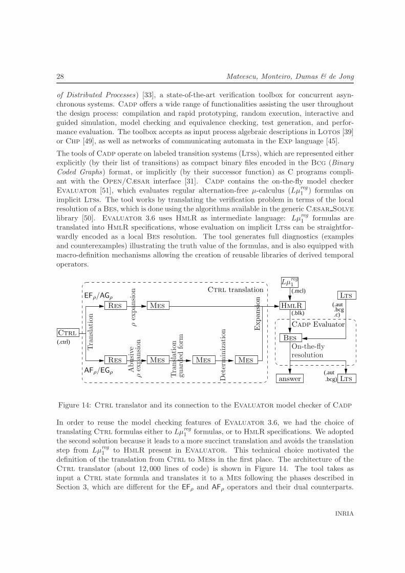
In order to reuse the model checking features of Evaluator 3.6, we had the choice oftranslating Ctrl formulas either to Lµreg
1 formulas, or to HmlR specifications. We adoptedthe second solution because it leads to a more succinct translation and avoids the translationstep from Lµreg
1 to HmlR present in Evaluator. This technical choice motivated thedefinition of the translation from Ctrl to Mess in the first place. The architecture of theCtrl translator (about 12, 000 lines of code) is shown in Figure 14. The tool takes asinput a Ctrl state formula and translates it to a Mes following the phases described inSection 3, which are different for the EFρ and AFρ operators and their dual counterparts.
INRIA
Computation Tree Regular Logic for Genetic Regulatory Networks 29
The Mes obtained is then converted into a HmlR specification by expanding the basicCtrl temporal operators in terms of Hml modalities as shown in Section 4.1. The resultingHmlR specification is directly given as input to Evaluator 3.6, together with the Ltscorresponding to the Kripke structure.
The translator from Ctrl to HmlR has been completely implemented, using the compilerconstruction technology based upon the Syntax3 system and the Lotos-Nt [34] languageproposed in [32], which was successfully used for developing several tools of Cadp.
5.2 Verification of genetic regulatory networks
Ctrl has been used for the analysis of so-called genetic regulatory networks (Grns), whichconsist of genes, proteins, small molecules and their mutual interactions that together controldifferent functions of the cell. In order to better understand how a specific dynamic behavioremerges from these interactions, and the role of each component in the network, a widevariety of mathematical formalisms are available. The description of the dynamics of Grnsby means of these formalisms results in qualitative or quantitative, discrete or continuous,stochastic or deterministic models [23].
Despite the enormous amount of information accumulated on the components and interac-tions of Grns, numerical values for the kinetic parameters and the molecular concentrationsare usually absent. As a consequence, the above-mentioned models of Grns are difficultto apply in practice. This has motivated the use of a special class of piecewise-linear (Pl)differential equation models, originally introduced by [35]. The Pl models provide a coarse-grained picture of the dynamics of Grns. They associate a protein concentration variableto each of the genes in the network, and capture the switch-like character of gene regula-tion by means of step functions that change their value at a threshold concentration of theproteins. The advantage of using the Pl models is that the qualitative dynamics of the high-dimensional systems are relatively straightforward to analyze, using inequality constraintson the parameters rather than exact numerical values [9, 24].
In [9] it is shown how discrete abstractions can be used to convert the continuous dynamics ofthe Pl systems into state transition graphs that are formally equivalent to Kripke structures.The states of the graph correspond to hyperrectangular regions in the concentration space,while the transitions arise from trajectories that enter one region from another. The atomicpropositions describe, among other things, the concentration bounds defining a region andthe trend of the variables inside the region (increasing, decreasing, or steady). The generationof the state transition graph from the Pl model has been implemented in the computer toolGna (Genetic Network Analyzer) [10]. Gna is able to export the graph to standard modelcheckers like NuSmv [20] and Cadp [33] in order to use formal verification techniques.
We analyse here properties of the carbon starvation response network in E. coli, using aPl model proposed in [55] (Figure 15). The dynamics of the system are described by 6coupled Pl differential equations, and 48 inequality constraints on the parameter values.We focus on one particular situation, a nutrient upshift after a period of starvation, leading
3Syntax is a trademark of INRIA.
RR n° 6521
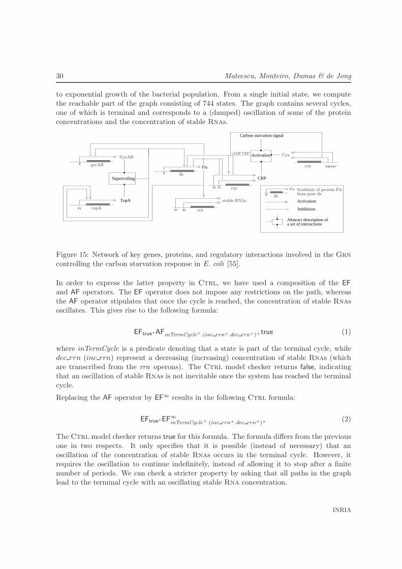
30 Mateescu, Monteiro, Dumas & de Jong
to exponential growth of the bacterial population. From a single initial state, we computethe reachable part of the graph consisting of 744 states. The graph contains several cycles,one of which is terminal and corresponds to a (damped) oscillation of some of the proteinconcentrations and the concentration of stable Rnas.
Activation
P1/P1’
CRP
PFis
P
P1 P2
P1 P2
TopA
P2
P1
Supercoiling
Activation
Abstract description ofa set of interactions
Inhibition
P
Carbon starvation signal
Synthesis of protein Fisfrom gene fis
GyrAB
gyrAB
topA
crp
cya
stable RNAs
cAMP·CRP Cya
rrn
fis
Fis
fis
Figure 15: Network of key genes, proteins, and regulatory interactions involved in the Grncontrolling the carbon starvation response in E. coli [55].
In order to express the latter property in Ctrl, we have used a composition of the EF
and AF operators. The EF operator does not impose any restrictions on the path, whereasthe AF operator stipulates that once the cycle is reached, the concentration of stable Rnasoscillates. This gives rise to the following formula:
EFtrue∗AFinTermCycle+.(inc rrn+.dec rrn+)+true (1)
where inTermCycle is a predicate denoting that a state is part of the terminal cycle, whiledec rrn (inc rrn) represent a decreasing (increasing) concentration of stable Rnas (whichare transcribed from the rrn operons). The Ctrl model checker returns false, indicatingthat an oscillation of stable Rnas is not inevitable once the system has reached the terminalcycle.
Replacing the AF operator by EF∞ results in the following Ctrl formula:
EFtrue∗EF∞inTermCycle+.(inc rrn+.dec rrn+)+
(2)
The Ctrl model checker returns true for this formula. The formula differs from the previousone in two respects. It only specifies that it is possible (instead of necessary) that anoscillation of the concentration of stable Rnas occurs in the terminal cycle. However, itrequires the oscillation to continue indefinitely, instead of allowing it to stop after a finitenumber of periods. We can check a stricter property by asking that all paths in the graphlead to the terminal cycle with an oscillating stable Rna concentration.
INRIA
Computation Tree Regular Logic for Genetic Regulatory Networks 31
AGtrue∗EF∞inTermCycle+.(inc rrn+.dec rrn+)+
(3)
Formula 3 is false, confirming that some paths do not end up in this cycle. However, we canimpose a path restriction on the AG operator, to force the model checker to consider onlysome of the paths:
AGtrue∗.inc F is+.dec Crp+.inTermCycleEF∞inTermCycle+.(inc rrn+.dec rrn+)+
(4)
The Ctrl model checker returns true for formula 4, proving that all paths satisfying therestriction of an increase of the Fis concentration and a decrease of the Crp concentration,reach the terminal cycle where the concentration of stable Rnas continues to oscillate.
The use of regular expressions in the above Ctrl formulas clearly demonstrates the con-venience of being able to characterize a sequence of events. Due to the nested iterationoperators present in the regular formulas, the Ctrl formulas cannot be expressed usingstandard temporal logics such as Ctl or Ltl. In addition, the EF∞
ρ operator enables a natu-ral formulation of infinite repetitions of sequences defined by ρ, such as those correspondingto oscillations in the E. coli example.
6 Conclusions and Future Work
Applications of model checking in system biology have demonstrated its usefulness for un-derstanding the dynamic behaviour of regulatory networks in living cells, but also outlinedcertain limitations in expressiveness and user-friendliness. Our work aims at alleviating theselimitations in order to promote the practical usage of model checking in the bioinformaticsand systems biology communities. The temporal logic Ctrl that we proposed, an extensionof Ctl with regular expressions and fairness operators, allows a natural and concise de-scription of typical properties of biological interest, such as the presence of multistability oroscillations in the concentrations of molecular species. We were able to obtain an on-the-flymodel checker for Ctrl by defining and implementing a translation from Ctrl to HmlR,and by reusing the verification and diagnostic generation features of the Evaluator 3.6model checker of Cadp. This modular architecture allowed us to reduce the developmenteffort and to take advantage of existing, robust model checking technology.
The extension of classical temporal logics with regular language constructs in order to in-crease their expressiveness and user-friendliness is a long-standing line of research. One ofthe first proposals in this direction was Etl [63], an extension of Ltl with regular gram-mars, which is strictly more expressive than Ltl while still having the same complexity ofevaluation on Kripke structures. Another manner of increasing expressiveness is to enhancetemporal operators with automata on infinite sequences; this was attempted for Ctl∗ [60]and Ctl [36]. Despite their expressive power, these extensions are difficult to implementand use in practice because of their complex syntax.
RR n° 6521
32 Mateescu, Monteiro, Dumas & de Jong
A more user-friendly approach, which led to successful implementations, is to index tempo-ral operators by regular expressions instead of automata. ForSpec [4] and Eagle [7] areextensions of Ltl with regular expressions and data handling mechanisms, dedicated respec-tively to hardware and runtime verification. Rctl [12] is an extension of Ctl with regularexpressions, which served subsequently as the basis of the Sugar [11] and Psl [38] speci-fication languages used for hardware verification. RegCtl [14] is another extension of Ctlwith regular expressions, more expressive than Rctl, obtained by indexing the Until oper-ator of Ctl with regular expressions. Our proposal is in line with these latter approaches,but focuses on the translation of Ctrl to the modal µ-calculus, which among other thingsallows us to reuse the on-the-fly verification technology available for the latter formalism.This contrasts with the model checking approaches proposed for the other extensions of Ctl,which are most of the time based on automata.
In this report, we have employed Ctrl for the verification of dynamic properties of Grnsmodeled by piecewise-linear differential equations. The continuous dynamics of these modelscan be converted into discrete state transition graphs that are formally equivalent to Kripkestructures. The computer tool Gna is able to generate the state transition graphs and exportthem as Kripke structures to Cadp. This allows the use of Cadp for verifying properties ofthe network expressed in Ctrl, as illustrated on the carbon starvation network in E. coli.
The application of Ctrl in systems biology and bioinformatics is not restricted to the classof models considered in this paper though. Ctrl is interpreted on Kripke structures, whichprovide a general description of dynamical systems that implicitly or explicitly underlie manyof the existing discrete formalisms used for the modeling of regulatory networks in the cell,such as Boolean networks and their generalizations, Petri nets, and process algebras [18, 29].In addition, other types of continuous models of regulatory networks, by defining appropriatediscrete abstractions, can possibly be mapped to Kripke structures as well. As a consequence,Ctrl can be combined with many of the other approaches proposed for the application offormal verification tools to biological regulatory networks [3, 6, 10, 13, 16, 17, 30].
We plan to continue our work on several directions. First, we will extend theCæsar Solve [50] library of Cadp with resolution algorithms handling Bess of alterna-tion depth 2 [61] in order to obtain an on-the-fly evaluation of the AF∞
ρ operator when theregular formula ρ is nondeterministic. Second, the translation from Ctrl to HmlR can beoptimized by adding static analysis features on the Gna atomic propositions in order toreduce the size of the HmlR specifications produced. Third, a distributed version of theCtrl model checker can be obtained by coupling it with the distributed Bes resolutionalgorithms proposed in [40, 41]. Fourth, we will develop tools to help non-expert users inapplying formal verification to the analysis of biological regulatory networks [53].
Acknowledgements
This research was funded by the Ec-Moan project no. 043235 of the Fp6-Nest-Path-ComEuropean program. Pedro T. Monteiro is also supported by the Fct program (PhD grantSfrh/Bd/32965/2006). Estelle Dumas is grateful to David Champelovier, Hubert Garavel,
INRIA
Computation Tree Regular Logic for Genetic Regulatory Networks 33
Romain Lacroix, and Michel Page for their valuable assistance in developing the translatorfrom Ctrl to HmlR.
References
[1] A. V. Aho, R. Sethi, and J. D. Ullman. Compilers: Principles, Techniques and Tools.Addison-Wesley, 1986.
[2] H. R. Andersen. Model checking and boolean graphs. Theoretical Computer Science,126(1):3–30, April 1994.
[3] M. Antoniotti, A. Policriti, N. Ugel, and B. Mishra. Model building and model checkingfor biochemical processes. Cell Biochemistry and Biophysics, 38(3):271–286, 2003.
[4] R. Armoni, L. Fix, A. Flaisher, R. Gerth, B. Ginsburg, T. Kanza, A. Landver, S. Mador-Haim, E. Singerman, A. Tiemeyer, M. Y. Vardi, and Y. Zbar. The ForSpec temporallogic: A new temporal property-specification language. In Joost-Pieter Katoen andPerdita Stevens, editors, Proceedings of the 8th International Conference on Tools andAlgorithms for the Construction and Analysis of Systems TACAS’02 (Grenoble, France),volume 2280 of Lecture Notes in Computer Science, pages 296–211. Springer Verlag,April 2002.
[5] T. Arts, C. Benac Earle, and J. Derrick. Development of a verified Erlang programfor resource locking. Springer International Journal on Software Tools for TechnologyTransfer (STTT), 5(2–3):205–220, March 2004.
[6] J. Barnat, L. Brim, I. Cerna, S. Drazan, and D. Safranek. Parallel model checking large-scale genetic regulatory networks with DiVinE. In From Biology to Concurrency andBack, FBTC 2007, volume 194 of Electronic Notes in Theoretical Computer Science,2008.
[7] H. Barringer, A. Goldberg, K. Havelund, and K. Sen. Rule-based runtime verification. InBernhard Steffen and Giorgio Levi, editors, Proceedings of the 5th International Confer-ence on Verification, Model Checking, and Abstract Interpretation VMCAI’04 (Venice,Italy), volume 2937 of Lecture Notes in Computer Science, pages 44–57. Springer Verlag,January 2004.
[8] G. Batt, D. Bergamini, H. de Jong, H. Gavarel, and R. Mateescu. Model checking geneticregulatory networks using GNA and CADP. In S. Graf and L. Mounier, editors, EleventhInternational SPIN Workshop on Model Checking of Software, SPIN 2004, volume 2989of Lecture Notes in Computer Science, pages 158–163, Berlin, 2004. Springer-Verlag.
[9] G. Batt, H. de Jong, M. Page, and J. Geiselmann. Symbolic reachability analysis ofgenetic regulatory networks using discrete abstractions. Automatica, 44(4):982–989,2008.
RR n° 6521
34 Mateescu, Monteiro, Dumas & de Jong
[10] G. Batt, D. Ropers, H. de Jong, J. Geiselmann, R. Mateescu, M. Page, and D. Schnei-der. Validation of qualitative models of genetic regulatory networks by model check-ing: Analysis of the nutritional stress response in Escherichia coli. Bioinformatics,21(Suppl 1):i19–i28, 2005.
[11] I. Beer, S. Ben-David, C. Eisner, D. Fisman, A. Gringauze, and Y. Rodeh. The temporallogic Sugar. In Gerard Berry, Hubert Comon, and Alain Finkel, editors, Proceedings ofthe 13th International Conference on Computer Aided Verification CAV’2001 (Paris,France), volume 2102 of Lecture Notes in Computer Science, pages 363–367. SpringerVerlag, July 2001.
[12] I. Beer, S. Ben-David, and A. Landver. On-the-fly model checking of RCTL formulas. InAlan Hu and Moshe Y. Vardi, editors, Proceedings of the 10th International Conferenceon Computer Aided Verification CAV’98 (Vancouver, BC, Canada), volume 1427 ofLecture Notes in Computer Science, pages 184–194. Springer Verlag, June 1998.
[13] G. Bernot, J.-P. Comet, A. Richard, and J. Guespin. Application of formal methods tobiological regulatory networks: Extending Thomas’ asynchronous logical approach withtemporal logic. Journal of Theoretical Biology, 229(3):339–348, 2004.
[14] T. Brazdil and I. Cerna. Model checking of RegCTL. Computers and Artificial Intelli-gence, 25(1), 2006.
[15] J. A. Brzozowski. Derivatives of regular expressions. J. ACM, 11(4):481–494, 1964.
[16] M. Calder, V. Vyshemirsky, D. Gilbert, and R. Orton. Analysis of signalling pathwaysusing the PRISM model checker. In G. Plotkin, editor, Computational Methods inSystems Biology, CMSB-05, pages 79–90, Edinburgh, Scotland, 2005.
[17] N. Chabrier-Rivier, M. Chiaverini, V. Danos, F. Fages, and V. Schachter. Modeling andquerying biomolecular interaction networks. Theoretical Computer Science, 325(1):25–44, 2004.
[18] C. Chaouiya. Petri net modelling of biological networks. Briefings in Bioinformatics,8(4):210–219, 2007.
[19] K.C. Chen, L. Calzone, A. Csikasz-Nagy, F.R. Cross, B. Novak, and J.J. Tyson. Inte-grative analysis of cell cycle control in budding yeast. Molecular Biology of the Cell,15(8):3841–3862, 2004.
[20] A. Cimatti, E. Clarke, F. Giunchiglia, and M. Roveri. NuSMV: a new symbolic modelchecker. Springer International Journal on Software Tools for Technology Transfer(STTT), 2(4):410–425, April 2000.
[21] E. Clarke, O. Grumberg, and D. Peled. Model Checking. MIT Press, 2000.
[22] R. Cleaveland and B. Steffen. A linear-time model-checking algorithm for thealternation-free modal mu-calculus. Formal Methods in System Design, 2(2):121–147,April 1993.
INRIA
Computation Tree Regular Logic for Genetic Regulatory Networks 35
[23] H. de Jong. Modeling and simulation of genetic regulatory systems: A literature review.Journal of Computational Biology, 9(1):67–103, 2002.
[24] H. de Jong, J.-L. Gouze, C. Hernandez, M. Page, T. Sari, and J. Geiselmann. Qualitativesimulation of genetic regulatory networks using piecewise-linear models. Bulletin ofMathematical Biology, 66(2):301–340, 2004.
[25] D. Dubnau and R. Losick. Bistability in bacteria. Molecular Microbiology, 61(3):564–572, 2006.
[26] E. A. Emerson and J. Y. Halpern. “Sometimes” and “not never” revisited: On branchingversus linear time. In Proceedings of the 10th Annual ACM Symposium on Principles ofProgramming Languages POPL’83 (Austin, Texas), pages 127–140, January 1983. Alsoappeared in Journal of ACM, 33(1):151-178, 1986.
[27] E. Allen Emerson and C-L. Lei. Efficient model checking in fragments of the propo-sitional mu-calculus. In Proceedings of the 1st International Symposium on Logic inComputer Science LICS’86, pages 267–278, 1986.
[28] M. J. Fischer and R. E. Ladner. Propositional dynamic logic of regular programs.Journal of Computer and System Sciences, 18(2):194–211, September 1979.
[29] J. Fisher and T.A. Henzinger. Executable cell biology. Nature Biotechnology,25(11):1239–1250, 2007.
[30] J. Fisher, N. Piterman, A. Hajnal, and T.A. Henzinger. Predictive modeling of signalingcrosstalk during C. elegans vulval development. PLoS Computational Biology, 3(5):e92,2007.
[31] H. Garavel. OPEN/CÆSAR: An open software architecture for verification, simulation,and testing. In Bernhard Steffen, editor, Proceedings of the First International Confer-ence on Tools and Algorithms for the Construction and Analysis of Systems TACAS’98(Lisbon, Portugal), volume 1384 of Lecture Notes in Computer Science, pages 68–84,Berlin, March 1998. Springer Verlag. Full version available as INRIA Research Re-port RR-3352.
[32] H. Garavel, F. Lang, and R. Mateescu. Compiler construction using LOTOS NT. InNigel Horspool, editor, Proceedings of the 11th International Conference on CompilerConstruction CC’2002 (Grenoble, France), volume 2304 of Lecture Notes in ComputerScience, pages 9–13. Springer Verlag, April 2002.
[33] H. Garavel, F. Lang, R. Mateescu, and W. Serwe. CADP 2006: A toolbox for theconstruction and analysis of distributed processes. In Werner Damm and Holger Her-manns, editors, Proceedings of the 19th International Conference on Computer AidedVerification CAV’2007 (Berlin, Germany), volume 4590 of Lecture Notes in ComputerScience, pages 158–163. Springer Verlag, July 2007.
RR n° 6521
36 Mateescu, Monteiro, Dumas & de Jong
[34] H. Garavel and M. Sighireanu. Towards a second generation of formal description tech-niques – rationale for the design of E-LOTOS. In Jan-Friso Groote, Bas Luttik, and Josvan Wamel, editors, Proceedings of the 3rd International Workshop on Formal Meth-ods for Industrial Critical Systems FMICS’98 (Amsterdam, The Netherlands), pages187–230, 1998.
[35] L. Glass and S.A. Kauffman. The logical analysis of continuous non-linear biochemicalcontrol networks. Journal of Theoretical Biology, 39(1):103–129, 1973.
[36] K. Hamaguchi, H. Hiraishi, and S. Yajima. Branching time regular temporal logicfor model checking with linear time complexity. In E. M. Clarke and R. P. Kurshan,editors, Proceedings of the 2nd International Conference on Computer Aided VerificationCAV’90 (New Brunswick, New Jersey, USA), volume 531 of Lecture Notes in ComputerScience, pages 253–262, Berlin, June 1990. Springer Verlag.
[37] G. Holzmann. The SPIN Model Checker – Primer and Reference Manual. Addison-Wesley, 2003.
[38] IEEE. PSL: Property specification language. Standard P1850, IEEE Computer Society,2004.
[39] ISO/IEC. LOTOS — a formal description technique based on the temporal ordering ofobservational behaviour. International Standard 8807, International Organization forStandardization — Information Processing Systems — Open Systems Interconnection,Geneve, September 1989.
[40] C. Joubert and R. Mateescu. Distributed local resolution of boolean equation systems.In Francisco Tirado and Manuel Prieto, editors, Proceedings of the 13th EuromicroConference on Parallel, Distributed and Network-Based Processing PDP’2005 (Lugano,Switzerland). IEEE Computer Society, 2005.
[41] C. Joubert and R. Mateescu. Distributed on-the-fly model checking and test case gen-eration. In Antti Valmari, editor, Proceedings of the 13th International SPIN Workshopon Model Checking of Software SPIN’2006 (Vienna, Austria), volume 3925 of LectureNotes in Computer Science, pages 126–145. Springer Verlag, March–April 2006.
[42] S. C. Kleene. Introduction to Metamathematics. North-Holland, 1952.
[43] E. Klipp, B. Nordlander, R. Kruger, P. Gennemark, and S. Hohmann. Integrative modelof the response of yeast to osmotic shock. Nature Biotechnology, 23(8):975–982, 2005.
[44] D. Kozen. Results on the propositional µ-calculus. Theoretical Computer Science,27:333–354, 1983.
[45] F. Lang. EXP.OPEN 2.0: A flexible tool integrating partial order, compositional, andon-the-fly verification methods. In Jaco van de Pol, Judi Romijn, and Graeme Smith,editors, Proceedings of the 5th International Conference on Integrated Formal MethodsIFM’2005 (Eindhoven, The Netherlands), volume 3771 of Lecture Notes in ComputerScience. Springer Verlag, 2005.
INRIA
Computation Tree Regular Logic for Genetic Regulatory Networks 37
[46] K. G. Larsen. Proof systems for Hennessy-Milner logic with recursion. In Proceedings ofthe 13th Colloquium on Trees in Algebra and Programming CAAP’88 (Nancy, France),volume 299 of Lecture Notes in Computer Science, pages 215–230, Berlin, March 1988.Springer Verlag.
[47] J.-C. Leloup and A. Goldbeter. Toward a detailed computational model for the mam-malian circadian clock. Proceedings of the National Academy of Sciences of the USA,100(12):7051–7056, 2003.
[48] Z. Manna and A. Pnueli. The Temporal Logic of Reactive and Concurrent Systems,volume I: Specification. Springer Verlag, 1992.
[49] A. J. Martin. Compiling communicating processes into delay-insensitive VLSI circuits.Distributed Computing, 1(4):226–234, 1986.
[50] R. Mateescu. CÆSAR SOLVE: A generic library for on-the-fly resolution of alternation-free boolean equation systems. Springer International Journal on Software Tools forTechnology Transfer (STTT), 8(1):37–56, February 2006. Full version available as IN-RIA Research Report RR-5948, July 2006.
[51] R. Mateescu and M. Sighireanu. Efficient on-the-fly model-checking for regularalternation-free mu-calculus. Science of Computer Programming, 46(3):255–281, March2003.
[52] R. Mateescu and D. Thivolle. A model checking language for concurrent value-passingsystems. In Proceedings of the 15th International Symposium on Formal Methods FM’08(Turku, Finland), 2008.
[53] P.T. Monteiro, D. Ropers, R. Mateescu, A.T. Freitas, and H. de Jong. Temporal logicpatterns for querying dynamic models of cellular interaction networks. Bioinformatics,2008. In press.
[54] A. Regev and E. Shapiro. Cells as computation. Nature, 419(6905):343, 2002.
[55] D. Ropers, H. de Jong, M. Page, D. Schneider, and J. Geiselmann. Qualitative simula-tion of the carbon starvation response in Escherichia coli. Biosystems, 84(2):124–152,2006.
[56] B. Schoeberl, C. Eichler-Jonsson, E.-D. Gilles, and G. Mller. Computational modelingof the dynamics of the MAP kinase cascade activated by surface and internalized EGFreceptors. Nature Biotechnology, 20(4):370–375, 2002.
[57] R. Streett. Propositional dynamic logic of looping and converse. Information andControl, 1982.
[58] A. Tarski. A lattice-theoretical fixpoint theorem and its applications. Pacific Journalof Mathematics, 5, 1955.
RR n° 6521
38 Mateescu, Monteiro, Dumas & de Jong
[59] R. Thomas, D. Thieffry, and M. Kaufman. Dynamical behaviour of biological regulatorynetworks: I. Biological role of feedback loops and practical use of the concept of theloop-characteristic state. Bulletin of Mathematical Biology, 57(2):247–276, 1995.
[60] W. Thomas. Computation Tree Logic and regular ω-languages, volume 354 of LectureNotes in Computer Science, pages 690–713. 1989.
[61] B. Vergauwen and J. Lewi. Efficient local correctness checking for single and alternatingboolean equation systems. In S. Abiteboul and E. Shamir, editors, Proceedings of the21st ICALP (Vienna), volume 820 of Lecture Notes in Computer Science, pages 304–315, Berlin, July 1994. Springer Verlag.
[62] P. Wolper. A translation from full branching time temporal logic to one letter proposi-tional dynamic logic with looping, 1982. Unpublished manuscript.
[63] P. Wolper. Temporal logic can be more expressive. Information and Control, 56(1/2):72–99, January-February 1983.
A Proofs of the translation
A.1 Translation from CTRL to RESs
A few additional definitions and lemmas are required in order to prove Proposition 1.Given a propositional environment δ = [U1/X1, ..., Un/Xn], its support is defined assupp(δ) = {X1, ...,Xn}, i.e., the set of variables that are mapped by δ to state sets. Itis straightforward to show that, for environments with disjoint supports, the ⊘ operator isassociative, commutative, and has the empty environment [ ] as neutral element. Moreover,supp([[B]]Kδ) = bv(B) and supp([[BL]]Kδ) = bv(BL) for any Kripke structure K, equationblock B, equation block list BL, and environment δ.
Lemma 2 Let K be a Kripke structure, B an equation block, and δ1, δ2 two propositionalenvironments such that supp(δ1) ∩ supp(δ2) = ∅ and fv(B) ⊆ supp(δ1). Then:
[[B]]K(δ1 ⊘ δ2) = [[B]]Kδ1.
Proof Let B = {Xiσ= ϕi}1≤i≤n be an equation block and δ1, δ2 two propositional environ-
ments as stated in the hypothesis. The semantics of B in the context of an environment δ isdetermined by the associated functional Φδ : (2S)n → (2S)n defined as follows:
Φδ(U1, ..., Un) = 〈[[ϕi]]K((δ1 ⊘ δ2) ⊘ [U1/X1, ..., Un/Xn])〉1≤i≤n
To prove the lemma, we show that the two functionals Φ(δ1⊘δ2) and Φδ1 are identical, i.e.,[[ϕ]]K((δ1 ⊘ δ2)⊘ [U1/X1, ..., Un/Xn]) = [[ϕ]]K(δ1 ⊘ [U1/X1, ..., Un/Xn]) for any formula ϕ andany U1, ..., Un ⊆ S. We proceed by structural induction on ϕ.
INRIA
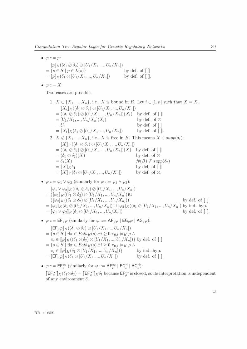
Computation Tree Regular Logic for Genetic Regulatory Networks 39� ϕ ::= p:
[[p]]K((δ1 ⊘ δ2) ⊘ [U1/X1, ..., Un/Xn])= {s ∈ S | p ∈ L(s)} by def. of [[ ]]= [[p]]K(δ1 ⊘ [U1/X1, ..., Un/Xn]) by def. of [[ ]].� ϕ ::= X:
Two cases are possible.
1. X ∈ {X1, ...,Xn}, i.e., X is bound in B. Let i ∈ [1, n] such that X = Xi.
[[Xi]]K((δ1 ⊘ δ2) ⊘ [U1/X1, ..., Un/Xn])= ((δ1 ⊘ δ2) ⊘ [U1/X1, ..., Un/Xn])(Xi) by def. of [[ ]]= [U1/X1, ..., Un/Xn](Xi) by def. of ⊘= Ui by def. of [ ]= [[Xi]]K(δ1 ⊘ [U1/X1, ..., Un/Xn]) by def. of [[ ]].
2. X 6∈ {X1, ...,Xn}, i.e., X is free in B. This means X ∈ supp(δ1).
[[X]]K((δ1 ⊘ δ2) ⊘ [U1/X1, ..., Un/Xn])= ((δ1 ⊘ δ2) ⊘ [U1/X1, ..., Un/Xn])(X) by def. of [[ ]]= (δ1 ⊘ δ2)(X) by def. of ⊘= δ1(X) fv(B) 6⊆ supp(δ2)= [[X]]Kδ1 by def. of [[ ]]= [[X]]K(δ1 ⊘ [U1/X1, ..., Un/Xn]) by def. of ⊘.� ϕ ::= ϕ1 ∨ ϕ2 (similarly for ϕ ::= ϕ1 ∧ ϕ2):
[[ϕ1 ∨ ϕ2]]K((δ1 ⊘ δ2) ⊘ [U1/X1, ..., Un/Xn])= ([[ϕ1]]K((δ1 ⊘ δ2) ⊘ [U1/X1, ..., Un/Xn]))∪
([[ϕ2]]K((δ1 ⊘ δ2) ⊘ [U1/X1, ..., Un/Xn])) by def. of [[ ]]= [[ϕ1]]K(δ1 ⊘ [U1/X1, ..., Un/Xn]) ∪ [[ϕ2]]K((δ1 ⊘ [U1/X1, ..., Un/Xn]) by ind. hyp.= [[ϕ1 ∨ ϕ2]]K(δ1 ⊘ [U1/X1, ..., Un/Xn]) by def. of [[ ]].� ϕ ::= EFρϕ (similarly for ϕ ::= AFρϕ | EGρϕ | AGρϕ):
[[EFρϕ]]K((δ1 ⊘ δ2) ⊘ [U1/X1, ..., Un/Xn])= {s ∈ S | ∃π ∈ PathK(s).∃i ≥ 0.π0,i |=K ρ ∧πi ∈ [[ϕ]]K((δ1 ⊘ δ2) ⊘ [U1/X1, ..., Un/Xn])} by def. of [[ ]]
= {s ∈ S | ∃π ∈ PathK(s).∃i ≥ 0.π0,i |=K ρ ∧πi ∈ [[ϕ]]K(δ1 ⊘ [U1/X1, ..., Un/Xn])} by ind. hyp.
= [[EFρϕ]]K(δ1 ⊘ [U1/X1, ..., Un/Xn]) by def. of [[ ]].� ϕ ::= EF∞ρ (similarly for ϕ ::= AF∞
ρ | EG⊣ρ | AG⊣
ρ ):
[[EF∞ρ ]]K(δ1⊘δ2) = [[EF∞
ρ ]]Kδ1 because EF∞ρ is closed, so its interpretation is independent
of any environment δ.
2
RR n° 6521
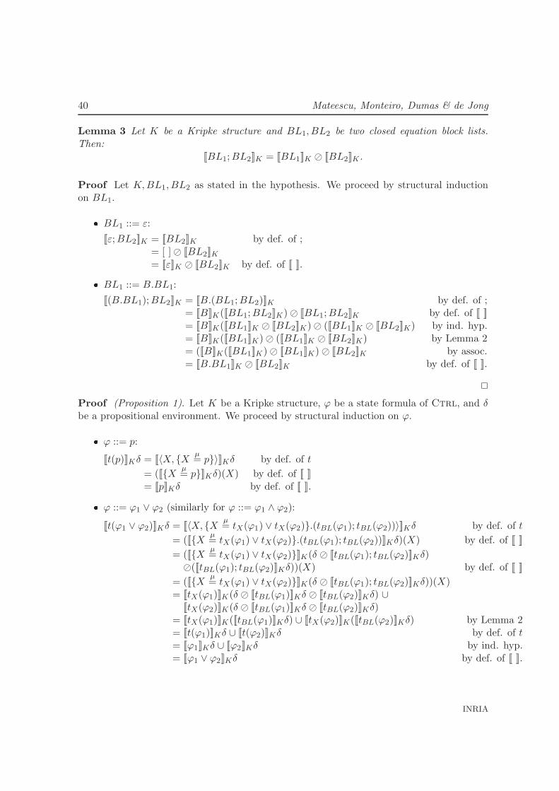
40 Mateescu, Monteiro, Dumas & de Jong
Lemma 3 Let K be a Kripke structure and BL1, BL2 be two closed equation block lists.Then:
[[BL1;BL2]]K = [[BL1]]K ⊘ [[BL2]]K .
Proof Let K,BL1, BL2 as stated in the hypothesis. We proceed by structural inductionon BL1.� BL1 ::= ε:
[[ε;BL2]]K = [[BL2]]K by def. of ;= [ ] ⊘ [[BL2]]K= [[ε]]K ⊘ [[BL2]]K by def. of [[ ]].� BL1 ::= B.BL1:
[[(B.BL1);BL2]]K = [[B.(BL1;BL2)]]K by def. of ;= [[B]]K([[BL1;BL2]]K) ⊘ [[BL1;BL2]]K by def. of [[ ]]= [[B]]K([[BL1]]K ⊘ [[BL2]]K) ⊘ ([[BL1]]K ⊘ [[BL2]]K) by ind. hyp.= [[B]]K([[BL1]]K) ⊘ ([[BL1]]K ⊘ [[BL2]]K) by Lemma 2= ([[B]]K([[BL1]]K) ⊘ [[BL1]]K) ⊘ [[BL2]]K by assoc.= [[B.BL1]]K ⊘ [[BL2]]K by def. of [[ ]].
2
Proof (Proposition 1). Let K be a Kripke structure, ϕ be a state formula of Ctrl, and δbe a propositional environment. We proceed by structural induction on ϕ.� ϕ ::= p:
[[t(p)]]Kδ = [[〈X, {Xµ= p}〉]]Kδ by def. of t
= ([[{Xµ= p}]]Kδ)(X) by def. of [[ ]]
= [[p]]Kδ by def. of [[ ]].� ϕ ::= ϕ1 ∨ ϕ2 (similarly for ϕ ::= ϕ1 ∧ ϕ2):
[[t(ϕ1 ∨ ϕ2)]]Kδ = [[〈X, {Xµ= tX(ϕ1) ∨ tX(ϕ2)}.(tBL(ϕ1); tBL(ϕ2))〉]]Kδ by def. of t
= ([[{Xµ= tX(ϕ1) ∨ tX(ϕ2)}.(tBL(ϕ1); tBL(ϕ2))]]Kδ)(X) by def. of [[ ]]
= ([[{Xµ= tX(ϕ1) ∨ tX(ϕ2)}]]K(δ ⊘ [[tBL(ϕ1); tBL(ϕ2)]]Kδ)
⊘([[tBL(ϕ1); tBL(ϕ2)]]Kδ))(X) by def. of [[ ]]
= ([[{Xµ= tX(ϕ1) ∨ tX(ϕ2)}]]K(δ ⊘ [[tBL(ϕ1); tBL(ϕ2)]]Kδ))(X)
= [[tX(ϕ1)]]K(δ ⊘ [[tBL(ϕ1)]]Kδ ⊘ [[tBL(ϕ2)]]Kδ) ∪[[tX(ϕ2)]]K(δ ⊘ [[tBL(ϕ1)]]Kδ ⊘ [[tBL(ϕ2)]]Kδ)
= [[tX(ϕ1)]]K([[tBL(ϕ1)]]Kδ) ∪ [[tX(ϕ2)]]K([[tBL(ϕ2)]]Kδ) by Lemma 2= [[t(ϕ1)]]Kδ ∪ [[t(ϕ2)]]Kδ by def. of t= [[ϕ1]]Kδ ∪ [[ϕ2]]Kδ by ind. hyp.= [[ϕ1 ∨ ϕ2]]Kδ by def. of [[ ]].
INRIA
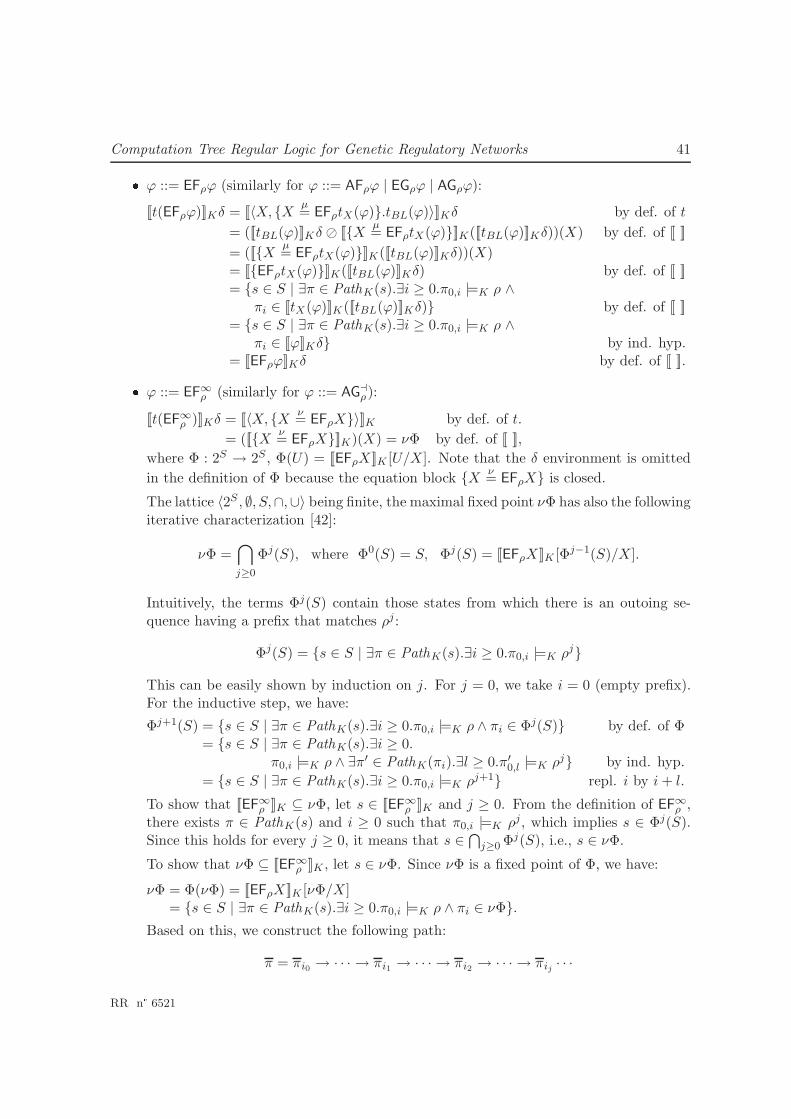
Computation Tree Regular Logic for Genetic Regulatory Networks 41� ϕ ::= EFρϕ (similarly for ϕ ::= AFρϕ | EGρϕ | AGρϕ):
[[t(EFρϕ)]]Kδ = [[〈X, {Xµ= EFρtX(ϕ)}.tBL(ϕ)〉]]Kδ by def. of t
= ([[tBL(ϕ)]]Kδ ⊘ [[{Xµ= EFρtX(ϕ)}]]K([[tBL(ϕ)]]Kδ))(X) by def. of [[ ]]
= ([[{Xµ= EFρtX(ϕ)}]]K([[tBL(ϕ)]]Kδ))(X)
= [[{EFρtX(ϕ)}]]K([[tBL(ϕ)]]Kδ) by def. of [[ ]]= {s ∈ S | ∃π ∈ PathK(s).∃i ≥ 0.π0,i |=K ρ ∧
πi ∈ [[tX(ϕ)]]K([[tBL(ϕ)]]Kδ)} by def. of [[ ]]= {s ∈ S | ∃π ∈ PathK(s).∃i ≥ 0.π0,i |=K ρ ∧
πi ∈ [[ϕ]]Kδ} by ind. hyp.= [[EFρϕ]]Kδ by def. of [[ ]].� ϕ ::= EF∞
ρ (similarly for ϕ ::= AG⊣ρ ):
[[t(EF∞ρ )]]Kδ = [[〈X, {X
ν= EFρX}〉]]K by def. of t.
= ([[{Xν= EFρX}]]K)(X) = νΦ by def. of [[ ]],
where Φ : 2S → 2S , Φ(U) = [[EFρX]]K [U/X]. Note that the δ environment is omitted
in the definition of Φ because the equation block {Xν= EFρX} is closed.
The lattice 〈2S , ∅, S,∩,∪〉 being finite, the maximal fixed point νΦ has also the followingiterative characterization [42]:
νΦ =⋂
j≥0
Φj(S), where Φ0(S) = S, Φj(S) = [[EFρX]]K [Φj−1(S)/X].
Intuitively, the terms Φj(S) contain those states from which there is an outoing se-quence having a prefix that matches ρj :
Φj(S) = {s ∈ S | ∃π ∈ PathK(s).∃i ≥ 0.π0,i |=K ρj}
This can be easily shown by induction on j. For j = 0, we take i = 0 (empty prefix).For the inductive step, we have:
Φj+1(S) = {s ∈ S | ∃π ∈ PathK(s).∃i ≥ 0.π0,i |=K ρ ∧ πi ∈ Φj(S)} by def. of Φ= {s ∈ S | ∃π ∈ PathK(s).∃i ≥ 0.
π0,i |=K ρ ∧ ∃π′ ∈ PathK(πi).∃l ≥ 0.π′0,l |=K ρj} by ind. hyp.
= {s ∈ S | ∃π ∈ PathK(s).∃i ≥ 0.π0,i |=K ρj+1} repl. i by i+ l.
To show that [[EF∞ρ ]]K ⊆ νΦ, let s ∈ [[EF∞
ρ ]]K and j ≥ 0. From the definition of EF∞ρ ,
there exists π ∈ PathK(s) and i ≥ 0 such that π0,i |=K ρj, which implies s ∈ Φj(S).Since this holds for every j ≥ 0, it means that s ∈
⋂
j≥0 Φj(S), i.e., s ∈ νΦ.
To show that νΦ ⊆ [[EF∞ρ ]]K , let s ∈ νΦ. Since νΦ is a fixed point of Φ, we have:
νΦ = Φ(νΦ) = [[EFρX]]K [νΦ/X]= {s ∈ S | ∃π ∈ PathK(s).∃i ≥ 0.π0,i |=K ρ ∧ πi ∈ νΦ}.
Based on this, we construct the following path:
π = πi0 → · · · → πi1 → · · · → πi2 → · · · → πij · · ·
RR n° 6521
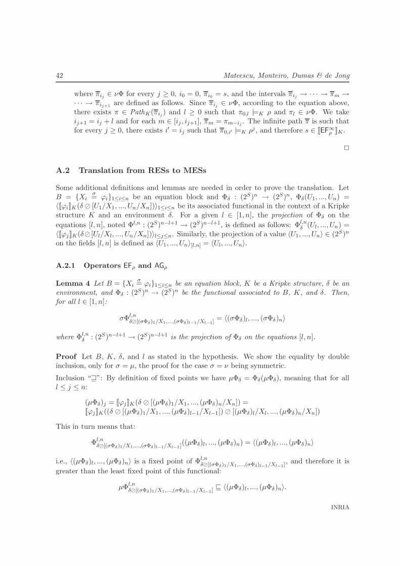
42 Mateescu, Monteiro, Dumas & de Jong
where πij ∈ νΦ for every j ≥ 0, i0 = 0, πi0 = s, and the intervals πij → · · · → πm →· · · → πij+1
are defined as follows. Since πij ∈ νΦ, according to the equation above,there exists π ∈ PathK(πij) and l ≥ 0 such that π0,l |=K ρ and πl ∈ νΦ. We takeij+1 = ij + l and for each m ∈ [ij , ij+1], πm = πm−ij . The infinite path π is such thatfor every j ≥ 0, there exists i′ = ij such that π0,i′ |=K ρj , and therefore s ∈ [[EF∞
ρ ]]K .
2
A.2 Translation from RESs to MESs
Some additional definitions and lemmas are needed in order to prove the translation. LetB = {Xi
σ= ϕi}1≤i≤n be an equation block and Φδ : (2S)n → (2S)n, Φδ(U1, ..., Un) =
〈[[ϕi]]K(δ⊘ [U1/X1, ..., Un/Xn])〉1≤i≤n be its associated functional in the context of a Kripkestructure K and an environment δ. For a given l ∈ [1, n], the projection of Φδ on the
equations [l, n], noted Φl,n : (2S)n−l+1 → (2S)n−l+1, is defined as follows: Φl,nδ (Ul, ..., Un) =
〈[[ϕj ]]K(δ⊘ [Ul/Xl, ..., Un/Xn])〉l≤j≤n. Similarly, the projection of a value 〈U1, ..., Un〉 ∈ (2S)n
on the fields [l, n] is defined as 〈U1, ..., Un〉[l,n] = 〈Ul, ..., Un〉.
A.2.1 Operators EFρ and AGρ
Lemma 4 Let B = {Xiσ= ϕi}1≤i≤n be an equation block, K be a Kripke structure, δ be an
environment, and Φδ : (2S)n → (2S)n be the functional associated to B, K, and δ. Then,for all l ∈ [1, n]:
σΦl,nδ⊘[(σΦδ)1/X1,...,(σΦδ)l−1/Xl−1]
= 〈(σΦδ)l, ..., (σΦδ)n〉
where Φl,nδ : (2S)n−l+1 → (2S)n−l+1 is the projection of Φδ on the equations [l, n].
Proof Let B, K, δ, and l as stated in the hypothesis. We show the equality by doubleinclusion, only for σ = µ, the proof for the case σ = ν being symmetric.
Inclusion “⊒”: By definition of fixed points we have µΦδ = Φδ(µΦδ), meaning that for alll ≤ j ≤ n:
(µΦδ)j = [[ϕj ]]K(δ ⊘ [(µΦδ)1/X1, ..., (µΦδ)n/Xn]) =[[ϕj ]]K((δ ⊘ [(µΦδ)1/X1, ..., (µΦδ)l−1/Xl−1]) ⊘ [(µΦδ)l/Xl, ..., (µΦδ)n/Xn])
This in turn means that:
Φl,nδ⊘[(σΦδ)1/X1,...,(σΦδ)l−1/Xl−1]((µΦδ)l, ..., (µΦδ)n) = 〈(µΦδ)l, ..., (µΦδ)n〉
i.e., 〈(µΦδ)l, ..., (µΦδ)n〉 is a fixed point of Φl,nδ⊘[(σΦδ)1/X1,...,(σΦδ)l−1/Xl−1], and therefore it is
greater than the least fixed point of this functional:
µΦl,nδ⊘[(σΦδ)1/X1,...,(σΦδ)l−1/Xl−1] ⊑ 〈(µΦδ)l, ..., (µΦδ)n〉.
INRIA
Computation Tree Regular Logic for Genetic Regulatory Networks 43
Inclusion “⊒”: We use the iterative characterization [42] of µΦδ on the finite lattice〈2S
n, ∅, Sn,⊓,⊔〉 (the operations ⊓ and ⊔ are the pairwise extensions of ∩ and ∪):
µΦδ =⋃
k≥0
Φkδ (∅
n), where Φ0δ(∅
n) = ∅n, Φk+1δ (∅n) = Φδ(Φ
kδ (∅
n)).
We show, by induction on k, that (Φkδ (∅
n))[l,n] ⊑ µΦl,nδ⊘[(σΦδ)1/X1,...,(σΦδ)l−1/Xl−1].
Base step. (Φ0δ(∅
n))[l,n] = (∅n)[l,n] = ∅n−l+1 ⊑ µΦl,nδ⊘[(σΦδ)1/X1,...,(σΦδ)l−1/Xl−1].
Inductive step. We have:(Φk+1
δ (∅n))[l,n] = (Φδ(Φkδ (∅
n)))[l,n]
= 〈[[ϕj ]]K(δ ⊘ [(Φkδ (∅
n))1/X1, ..., (Φkδ (∅
n))n/Xn])〉l≤j≤n by def. of Φ= 〈[[ϕj ]]K((δ ⊘ [(Φk
δ (∅n))1/X1, ..., (Φ
kδ (∅
n))l−1/Xl−1]) ⊘[(Φk
δ (∅n))l/Xl, ..., (Φ
kδ (∅
n))n/Xn])〉l≤j≤n⊑ 〈[[ϕj ]]K((δ ⊘ [(µΦδ)1/X1, ..., (µΦδ)l−1/Xl−1]) ⊘
[(Φkδ (∅
n))l/Xl, ..., (Φkδ (∅
n))n/Xn])〉l≤j≤n by monotonicity
= Φl,nδ⊘[(µΦδ)1/X1,...,(µΦδ)l−1/Xl−1]
((Φkδ (∅
n))l, ..., (Φkδ (∅
n))n) by def. of Φl,n
= Φl,nδ⊘[(µΦδ)1/X1,...,(µΦδ)l−1/Xl−1]((Φ
kδ (∅
n))[l,n])
⊑ Φl,nδ⊘[(µΦδ)1/X1,...,(µΦδ)l−1/Xl−1](µΦl,n
δ⊘[(σΦδ)1/X1,...,(σΦδ)l−1/Xl−1]) by ind. hyp.
= µΦl,nδ⊘[(σΦδ)1/X1,...,(σΦδ)l−1/Xl−1] by def. of µ.
Thus, (µΦδ)[l,n] = (⋃
k≥0 Φkδ (∅
n))[l,n] =⋃
k≥0(Φkδ (∅
n))[l,n] ⊑ µΦl,nδ⊘[(σΦδ)1/X1,...,(σΦδ)l−1/Xl−1],
which concludes the proof. 2
The following lemma allows to replace an equation of a block by a set of equations, providedthat the interpretation of the variable in the left-hand side of the equation remains unchangedin the original and the substituting block w.r.t. all environments.
Lemma 5 (Substitution) Let B = {Xiσ= ϕi}1≤i≤n be an equation block, and let {Xn
σ=
ψn, Yjσ= ψj}n<j≤m be another block suitable for the substitution of the equation Xn
σ= ϕn
such that ([[{Xnσ= ϕn}]]Kδ)(Xn) = ([[{Xn
σ= ψn, Yj
σ= ψj}n<j≤m]]Kδ)(Xn) for any Kripke
structure K and environment δ. Then:
([[{Xiσ= ϕi}1≤i≤n[Xn
σ= ϕn := Xn
σ= ψn, Yj
σ= ψj ]n<j≤m]]Kδ)(Xi) = ([[{Xi
σ= ϕi}1≤i≤n]]Kδ)(Xi)
for all i ∈ [1, n] and for any K, δ.
Proof We show the lemma for σ = µ, the proof for the case σ = ν being symmetric. LetΦ1,mδ : (2S)m → (2S)m be the functional associated to the substituted equation block, defined
as follows:
Φ1,mδ (U1, ..., Un,Wn+1, ...,Wn) =
〈[[ϕi]]K(δ ⊘ [U1/X1, ..., Un/Xn,Wn+1/Yn+1, ...,Wm/Ym]),[[ψj ]]K(δ ⊘ [U1/X1, ..., Un/Xn,Wn+1/Yn+1, ...,Wm/Ym])〉1≤i<n,n≤j≤m
We first show that 〈(µΦ1,mδ )1, ..., (µΦ1,m
δ )n〉 is a fixed point of the functional Φδ as-
sociated to B and δ. From the definition of µΦ1,mδ , it follows that [[ϕi]]K(δ ⊘
RR n° 6521
44 Mateescu, Monteiro, Dumas & de Jong
[(µΦ1,mδ )1/X1, ..., (µΦ1,m
δ )n/Xn, (µΦ1,mδ )n+1/Yn+1, ..., (µΦ1,m
δ )m/Ym]) = (µΦ1,mδ )i for all i ∈
[1, n − 1]. The suitability condition⋃ni=1 fv(ϕi) ∩ {Yn+1, ..., Ym} = ∅ implies that all
formulas ϕi for i ∈ [1, n − 1] depend only upon X1, ...,Xn and therefore [[ϕi]]K(δ ⊘[(µΦ1,m
δ )1/X1, ..., (µΦ1,mδ )n/Xn]) = (µΦ1,m
δ )i. To show that this equality also holds for i = n,we apply Lemma 4 for l = n on the substituted block and we obtain:
µΦn,m
δ⊘[(µΦ1,mδ
)1/X1,...,(µΦ1,mδ
)n−1/Xn−1]= 〈(µΦ1,m
δ )n, ..., (µΦ1,mδ )m〉
where Φn,mδ : (2S)m−n+1 → (2S)m−n+1 is the projection of Φ1,m
δ on the equations [n,m].
From the hypothesis of the lemma and the definition of the interpretation [[{Xnσ= ψn, Yj
σ=
ψj}n<j≤m]]Kδ, this implies:
([[{Xnσ= ϕn}]]K(δ ⊘ [(µΦ1,m
δ )1/X1, ..., (µΦ1,mδ )n−1/Xn−1]))(Xn) = (µΦ1,m
δ )n
or, according to the definition of [[{Xnσ= ϕn}]]Kδ:
µΦnδ⊘[(µΦ1,m
δ )1/X1,...,(µΦ1,mδ )n−1/Xn−1]
= (µΦ1,mδ )n
where Φnδ : 2S → 2S , Φn
δ (U) = [[ϕn]]K(δ ⊘ [U/Xn]). Since (µΦ1,mδ )n is by definition a fixed
point of Φnδ⊘[(µΦ1,m
δ)1/X1,...,(µΦ1,m
δ)n−1/Xn−1]
, this means:
([[ϕn]]K((δ ⊘ [(µΦ1,mδ )1/X1, ..., (µΦ1,m
δ )n−1/Xn−1]) ⊘ [(µΦ1,mδ )n/Xn]))((µΦ1,m
δ )n) = (µΦ1,mδ )n
i.e.,([[ϕn]]K(δ ⊘ [(µΦ1,m
δ )1/X1, ..., (µΦ1,mδ )n/Xn]))((µΦ1,m
δ )n) = (µΦ1,mδ )n.
Therefore, 〈(µΦ1,mδ )i〉1≤i≤n is a fixed point of Φδ.
It remains to show that this is indeed the minimal fixed point of Φδ. Since the lattice〈2S
m, ∅, Sm,⊓,⊔〉 is finite (the operations ⊓ and ⊔ being the pairwise extensions of ∩ and
∪), the minimal fixed point µΦ1,mδ also has an iterative characterization [42]:
µΦ1,mδ =
⋃
k≥0
(Φ1,mδ )k(∅m), where (Φ1,m
δ )0(∅m) = ∅m, (Φ1,mδ )k+1(∅m) = Φ1,m
δ ((Φ1,mδ )k(∅m)).
We show, by induction on k, that ((Φ1,mδ )k(∅m))i ⊆ (µΦδ)i for all i ∈ [1, n] and k ≥ 0. Let
i ∈ [1, n].Base step. ((Φ1,m
δ )0(∅m))i = ∅ ⊆ (µΦδ)i.Inductive step. For i ∈ [1, n − 1], we have:
((Φ1,mδ )k+1(∅m))i = (Φ1,m
δ ((Φ1,mδ )k(∅m)))i
= [[ϕi]]K(δ ⊘ [((Φ1,mδ )k(∅m))1/X1, ..., ((Φ
1,mδ )k(∅m))m/Ym]) by def. of [[ ]]
= [[ϕi]]K(δ ⊘ [((Φ1,mδ )k(∅m))1/X1, ..., ((Φ
1,mδ )k(∅m))n/Xn]) by suitability
⊆ [[ϕi]]K(δ ⊘ [(µΦδ)1/X1, ..., (µΦδ)n/Xn]) by ind. hyp.= (µΦδ)i by def. of µΦδ.
For i = n, we have:
INRIA
Computation Tree Regular Logic for Genetic Regulatory Networks 45
((Φ1,mδ )k+1(∅m))n = [[ψn]]K(δ ⊘ [((Φ1,m
δ )k(∅m))1/X1, ..., ((Φ1,mδ )k(∅m))m/Ym])
⊆ [[ψn]]K(δ ⊘ [((Φ1,mδ )k(∅m))1/X1, ..., ((Φ
1,mδ )k(∅m))n−1/Xn−1,
(µΦ1,mδ )n/Xn, ..., (µΦ1,m
δ )m/Ym]) by def. µΦ1,mδ
= ([[{Xnµ= ψn, Yj
µ= ψj}n<j≤m]]K
(δ ⊘ [((Φ1,mδ )k(∅m))1/X1, ..., ((Φ
1,mδ )k(∅m))n−1/Xn−1]))(Xn) by def. of [[ ]]
= ([[Xnµ= ϕn]]K
(δ ⊘ [((Φ1,mδ )k(∅m))1/X1, ..., ((Φ
1,mδ )k(∅m))n−1/Xn−1]))(Xn) by hyp.
= µΦnδ⊘[((Φ1,m
δ )k(∅m))1/X1,...,((Φ1,mδ )k(∅m))n−1/Xn−1]
by def. of [[ ]]
⊆ µΦnδ⊘[(µΦδ)1/X1,...,(µΦδ)n−1/Xn−1] by ind. hyp.
= (µΦδ)n by Lemma 4.
The last application of Lemma 4 above considers the block B = {Xiσ= ϕi}1≤i≤n and takes
l = n. This concludes the proof that 〈(µΦ1,mδ )i〉1≤i≤n is the least fixed point of Φδ. 2
Lemma 5 allows to prove the correctness of a substitution by focusing only on the equationsinvolved in the substitution, as illustrated in the proof below.
Proof (Proposition 2). Let K be a Kripke structure, B1 = {Xiµ= ϕi}1≤i≤n and B2 =
{Xiν= ϕi}1≤i≤n two equation blocks, and δ a propositional environment as stated in the
hypothesis. We show the proposition only for blocks of type B1 and the substitutions in theupper part of Figure 5, the other cases being dual.� Substitution X
µ= EFρ1.ρ2Y := X
µ= EFρ1Z,Z
µ= EFρ2Y . It is sufficient to show that
this substitution satisfies the condition in the hypothesis of Lemma 5:
([[{Xµ= EFρ1.ρ2Y }]]Kδ)(X) = ([[{X
µ= EFρ1Z,Z
µ= EFρ2Y }]]Kδ)(X).
By applying the definition of [[ ]] and simple properties about substitution of variablesin a Res, we obtain:
([[{Xµ= EFρ1.ρ2Y }]]Kδ)(X)
= [[EFρ1.ρ2Y ]]Kδ= {s ∈ S | ∃π ∈ PathK(s).∃i ≥ 0.π0,i |=K ρ1.ρ2 ∧ πi ∈ [[Y ]]K}= {s ∈ S | ∃π ∈ PathK(s).∃i ≥ 0.∃k ∈ [0, i].π0,k |=K ρ1 ∧ πk,i |=K ρ2 ∧ πi ∈ [[Y ]]K}= {s ∈ S | ∃π ∈ PathK(s).∃k ≥ 0.π0,k |=K ρ1 ∧ ∃i ≥ k.πk,i |=K ρ2 ∧ πi ∈ [[Y ]]K}= {s ∈ S | ∃π ∈ PathK(s).∃k ≥ 0.π0,k |=K ρ1 ∧ ∃π′ ∈ PathK(πk).∃i ≥ k.
π′k,i |=K ρ2 ∧ π′i ∈ [[Y ]]K}
= {s ∈ S | ∃π ∈ PathK(s).∃k ≥ 0.π0,k |=K ρ ∧ πk ∈ [[EFρ2Y ]]K}= [[EFρ1EFρ2Y ]]Kδ
= ([[{Xµ= EFρ1EFρ2Y }]]Kδ)(X)
= ([[{Xµ= EFρ1Z,Z
µ= EFρ2Y }]]Kδ)(X).
RR n° 6521
46 Mateescu, Monteiro, Dumas & de Jong� Substitution Xµ= EFρ1|ρ2Y := X
µ= Z ∨ U,Z
µ= EFρ1Y,U
µ= EFρ2Y . As above, it is
sufficient to show that:
([[{Xµ= EFρ1|ρ2Y }]]Kδ)(X) = ([[{X
µ= Z ∨ U,Z
µ= EFρ1Y,U
µ= EFρ2Y }]]Kδ)(X).
By applying the definition of [[ ]] and simple properties about substitution of variablesin a Res, we obtain:
([[{Xµ= EFρ1|ρ2Y }]]Kδ)(X)
= [[EFρ1|ρ2Y ]]Kδ
= {s ∈ S | ∃π ∈ PathK(s).∃i ≥ 0.π0,i |=K ρ1|ρ2 ∧ πi ∈ [[Y ]]Kδ}= {s ∈ S | ∃π ∈ PathK(s).∃i ≥ 0.(π0,i |=K ρ1 ∨ π0,i |=K ρ2) ∧ πi ∈ [[Y ]]Kδ}= {s ∈ S | ∃π ∈ PathK(s).∃i ≥ 0.((π0,i |=K ρ1 ∧ πi ∈ [[Y ]]Kδ) ∨
(π0,i |=K ρ2 ∧ πi ∈ [[Y ]]Kδ))}= {s ∈ S | ∃π ∈ PathK(s).∃i ≥ 0.π0,i |=K ρ1 ∧ πi ∈ [[Y ]]Kδ ∨
∃π ∈ PathK(s).∃i ≥ 0.π0,i |=K ρ2 ∧ πi ∈ [[Y ]]Kδ}= [[EFρ1Y ∨ EFρ2Y ]]Kδ
= ([[{Xµ= EFρ1Y ∨ EFρ2Y }]]Kδ)(X)
= ([[{Xµ= Z ∨ U,Z
µ= EFρ1Y,U
µ= EFρ2Y }]]Kδ)(X).� Substitution X
µ= EFρ∗Y := X
µ= Y ∨ Z,Z
µ= EFρX. As above, it is sufficient to show
that:([[{X
µ= EFρ∗Y }]]Kδ)(X) = ([[{X
µ= Y ∨ Z,Z
µ= EFρX}]]Kδ)(X).
Let A = ([[{Xµ= EFρ∗Y }]]Kδ)(X). We have:
([[{Xµ= EFρ∗Y }]]Kδ)(X) = by def. of [[ ]]
[[EFρ∗Y ]]Kδ ={s ∈ S | ∃π ∈ PathK(s).∃i ≥ 0.π0,i |=K ρ∗ ∧ πi ∈ [[Y ]]Kδ} ={s ∈ S | ∃π ∈ PathK(s).∃i ≥ 0.∃k ≥ 0.π0,i |=K ρk ∧ πi ∈ δ(Y )}.
Let B = ([[{Xµ= Y ∨ Z,Z
µ= EFρX}]]Kδ)(X). We have:
([[{Xµ= Y ∨ Z,Z
µ= EFρX}]]Kδ)(X) = by subst. on Y
([[{Xµ= Y ∨ EFρX}]]Kδ)(X) = µΦδ
where the functional Φδ : 2S → 2S is defined as follows:
Φδ(U) = [[Y ∨ EFρX]]K(δ ⊘ [U/X])= [[Y ]]K(δ ⊘ [U/X]) ∪ [[EFρX]]K(δ ⊘ [U/X])= δ(Y ) ∪ [[EFρX]]K [U/X].
The lattice 〈2S , ∅, S,∩,∪〉 being finite, the minimal fixed point µΦδ has also the fol-lowing iterative characterization [42]:
µΦδ =⋃
k≥0
Φk(∅), where Φ0(∅) = ∅, Φk+1(∅) = δ(Y ) ∪ [[EFρX]]K [Φk(∅)/X].
INRIA
Computation Tree Regular Logic for Genetic Regulatory Networks 47
Intuitively, Φk+1(∅) contains those states having an outgoing sequence that matchesρj for some j ∈ [0, k] and leads to a state in δ(Y ):
Φk+1(∅) = {s ∈ S | ∃π ∈ PathK(s).∃i ≥ 0.∃j ∈ [0, k].π0,i |=K ρj ∧ πi ∈ δ(Y )}.
This statement can be easily shown by induction on k.Base step.Φ1(∅) = δ(Y ) ∪ [[EFρX]]K [Φ0(∅)/X]
= δ(Y ) ∪ [[EFρX]]K [∅/X]= δ(Y )= {s ∈ S | ∃π ∈ PathK(s).π0,0 |=K ρ0 ∧ π0 ∈ δ(Y )} by choosing i, j = 0.
Inductive step.Φk+2(∅) = Φ(Φk+1(∅)) by def. of Φ
= δ(Y ) ∪ {s ∈ S | ∃π ∈ PathK(s).∃i ≥ 0.π0,i |=K ρ ∧ πi ∈ Φk+1(∅)} by ind. hyp.
= δ(Y ) ∪ {s ∈ S | ∃π ∈ PathK(s).∃i ≥ 0.π0,i |=K ρ ∧∃π′ ∈ PathK(πi).∃i
′ ≥ 0.∃j ∈ [0, k].π′0,i′ |=K ρj ∧ π′i′ ∈ δ(Y )}
= δ(Y ) ∪ {s ∈ S | ∃π ∈ PathK(s).∃i ≥ 0.∃j ∈ [0, k].π0,i |=K ρj+1 ∧ πi ∈ δ(Y )} repl. i by i+ i′
= δ(Y ) ∪ {s ∈ S | ∃π ∈ PathK(s).∃i ≥ 0.∃j ∈ [1, k + 1].π0,i |=K ρj ∧ πi ∈ δ(Y )}
= {s ∈ S | ∃π ∈ PathK(s).∃i ≥ 0.∃j ∈ [0, k + 1].π0,i |=K ρj ∧ πi ∈ δ(Y )}.
From the above statement, we obtain:
B =⋃
k≥0 Φk(∅) = Φ0(∅) ∪⋃
k≥0 Φk+1(∅) =⋃
k≥0 Φk+1(∅)
=⋃
k≥0{s ∈ S | ∃π ∈ PathK(s).∃i ≥ 0.∃j ∈ [0, k].π0,i |=K ρj ∧ πi ∈ δ(Y )}
= {s ∈ S | ∃k ≥ 0.∃π ∈ PathK(s).∃i ≥ 0.∃j ∈ [0, k].π0,i |=K ρj ∧ πi ∈ δ(Y )}= {s ∈ S | ∃π ∈ PathK(s).∃i ≥ 0.∃k ≥ 0.∃j ∈ [0, k].π0,i |=K ρj ∧ πi ∈ δ(Y )}= {s ∈ S | ∃π ∈ PathK(s).∃i ≥ 0.∃k ≥ 0.π0,i |=K ρk ∧ πi ∈ δ(Y )} choose j = k= A.
2
A.2.2 Operators AFρ and EGρ
Translation to guarded form
Proof (Lemma 1). Let K be a Kripke structure, B = {Xiµ= ϕi}1≤i≤n be an equation block
and δ a propositional environment as stated in the hypothesis. It is sufficient to show thatthe absorption substitution satisfies the condition in the hypothesis of Lemma 5:
([[{Xµ= X ∨ ϕ}]]Kδ)(X) = ([[{X
µ= ϕ}]]Kδ)(X)
RR n° 6521
48 Mateescu, Monteiro, Dumas & de Jong
which amounts to show, applying the definition of [[ ]], that:
µΦδ = [[ϕ]]Kδ
where the functional Φδ : 2S → 2S is defined as Φδ(U) = [[X ∨ϕ]]K(δ⊘ [U/X]) = U ∪ [[ϕ]]Kδ.The lattice 〈2S , ∅, S,∩,∪〉 being finite, the minimal fixed point µΦδ has also the followingiterative characterization [42]:
µΦδ =⋃
k≥0
Φk(∅), where Φ0δ(∅) = ∅, Φk+1
δ (∅) = Φkδ (∅) ∪ [[ϕ]]Kδ.
To obtain the desired equality, it is therefore sufficient to show that Φk+1δ (∅) = [[ϕ]]Kδ for
every k ≥ 0. We proceed by induction on k.
Base step: Φ1δ(∅) = Φ0
δ(∅) ∪ [[ϕ]]Kδ = [[ϕ]]Kδ.
Inductive step:
Φk+1δ (∅) = Φk
δ (∅) ∪ [[ϕ]]Kδ by def.= [[ϕ]]Kδ ∪ [[ϕ]]Kδ by ind. hyp.= [[ϕ]]Kδ.
2
Determinization
Several definitions and lemmas are needed in order to prove Proposition 3. Consider a Kripkestructure K and the following potentiality Res:
Xiµ=
n∨
j=1
(hij ∧ EFρijXj) ∨ (hi ∧ Y )
1≤i≤n
(∗)
where hij , hi ∈ Bool and ρij are regular formulas for all 1 ≤ i, j ≤ n. Unguarded occurrencesof variables Xj in the right-hand sides of the equations are obtained by taking ρij = nil.Ress of the form (∗) are encountered throughout the translation from a potentiality Res
to its guarded form. For instance, a potentiality Res {X1µ= EFρY } can be rewritten as
{X1µ= EFρX2,X2
µ= Y }, which is in the form above by considering n = 2, h11 = false,
h12 = true, ρ12 = ρ, h1 = false, h21 = h22 = false, and h2 = true. Similarly, a guardedpotentiality Res is a particular case of form (∗) in which all regular formulas ρij are simplyatomic propositions pij.
To each propositional variable Xi of the potentiality Res (∗) and environment δ is associateda path predicate Pδ,i : PathK → Bool characterizing the paths denoted by Xi in the contextof δ. These path predicates are defined by the following equation system:
Pδ,i(π)µ=
n∨
j=1
(
hij ∧ ∃lij ≥ 0.π0,lij |= ρij ∧ Pδ,j(πlij ,∞))
∨ (hi ∧ π0 ∈ δ(Y ))
1≤i≤n
INRIA
Computation Tree Regular Logic for Genetic Regulatory Networks 49
where πlij ,∞ denotes the suffix of path π starting at the state of index lij .
The translation from a potentiality Mes {X1µ= EFρY } to its guarded form preserves the
path predicate associated to the main variable X1, as shown by the lemma below.
Lemma 6 Let K be a Kripke structure, R = {X1µ= EFρY } be an equation block, M be
its corresponding guarded potentiality Mes in the form (∗), and Pδ,i be its associated pathpredicates. Then:
Pδ,1(π) = ∃l ≥ 0.π0,l |= ρ ∧ πl ∈ δ(Y )
for any π ∈ PathK and any propositional environment δ.
Proof Let K be a Kripke structure and δ be a propositional environment. Let the equationblock R = {X1
µ= EFρX2,X2
µ= Y } in form (∗). Its associated path predicates are defined as
follows:Pδ,1(π) = ∃l12 ≥ 0.π0,l12 |= ρ12 ∧ Pδ,2(πl12,∞)Pδ,2(π) = π0 ∈ δ(Y )
where π ∈ PathK . After appropriate renamings, we obtain the desired equality:
Pδ,1(π) = ∃l ≥ 0.π0,l |= ρ ∧ πl ∈ δ(Y ).
It remains to show that this equality also holds along the translation of R into guardedform. This translation consists of two phases: elimination of the regular operators presentin ρ (Proposition 2) and elimination of unguarded occurrences of variables (Lemma 1).The substitutions performed in both phases preserve the path predicates associated to thevariables defined by the substituted equations. This can be shown using similar argumentsas in Proposition 2 and Lemma 1; we show below the path predicate preservation only forthe first rule in Proposition 2, leaving the other ones as exercises for the interested reader.
This rule transforms the Res R = {Xµ= EFρ1.ρ2Y } into the Res R′ = {X
µ= EFρ1Z,Z
µ=
EFρ2Y }. The predicate P ′δ,1 associated to X1 in R′ is defined as follows:
P ′δ,1(π) = ∃l ≥ 0.π0,l |= ρ1 ∧ P
′δ,2(πl,∞) by def. of P ′
δ,1
= ∃l ≥ 0.π0,l |= ρ1 ∧ ∃l′ ≥ 0.πl,l+l′ |= ρ2 ∧ πl+l′ ∈ δ(Y ) by def. of P ′δ,2
= ∃l ≥ 0.∃l′ ≥ 0.π0,l |= ρ1 ∧ πl,l+l′ |= ρ2 ∧ πl+l′ ∈ δ(Y )= ∃k ≥ 0.∃j ≥ 0.π0,j |= ρ1 ∧ πj,k |= ρ2 ∧ πk ∈ δ(Y ) by taking k = l + l′ and j = l= ∃k ≥ 0.∃j ≥ 0.π0,j |= ρ1 ∧ πj,k |= ρ2 ∧ πk ∈ δ(Y ) by def. of ρ1.ρ2
which coincides with the definition of Pδ,1 in R. Thus, the path predicate Pδ,1 associated toX1 in R remains unchanged during the translation of R into guarded form, which shows thedesired equality. 2
The relation between the path predicates associated to a guarded potentiality Mes and theinterpretation of the corresponding determinized Mes is given by the lemma below.
RR n° 6521
50 Mateescu, Monteiro, Dumas & de Jong
Lemma 7 Let K be a Kripke structure, M be a guarded potentiality Mes in the form (∗),and Pδ,i be its associated path predicates. The determinized Mes corresponding to M isdefined as in Section 3.2.2. Then:
([[{
XIµ=∨
∅⊂Q⊆prop(I) AFQXvars(Q,I) ∨ (h(I) ∧ Y )}
I⊆[1,n]
]]
Kδ)
(XJ )
={s ∈ S | ∀π ∈ PathK(s).∃j ∈ J.Pδ,j(π)}
for any index set J ⊆ [1, n] and any propositional environment δ.
Proof Let K, M , δ, and Pδ,i as stated in the hypothesis. The functional Φδ : (2S)2n−1
→
(2S)2n−1
associated to the determinized Mes corresponding to M is defined as follows:
Φδ(〈UJ 〉J⊆[1,n]) =⟨[[
∨
∅⊂Q⊆prop(I) AFQXvars(Q,I) ∨ (h(I) ∧ Y )]]
K(δ ⊘ [UJ/XJ ]J⊆[1,n])
⟩
I⊆[1,n]
The interpretation of the determinized Mes is equal to µΦδ. Let U = 〈{s ∈ S | ∀π ∈PathK(s).∃j ∈ J.Pδ,j(π)}〉J⊆[1,n]. We must show that µΦδ = U , which we split into a doubleinclusion.
Inclusion ⊆. By Tarski’s theorem [58], showing that µΦδ ⊆ U amounts to show thatΦδ(U) ⊆ U . We have:
Φδ(U) =⟨ [[
∨
∅⊂Q⊆prop(I) AFQXvars(Q,I) ∨ (h(I) ∧ Y )]]
K
(δ ⊘ [{s ∈ S | ∀π ∈ PathK(s).∃j ∈ J.Pδ,j(π)}/XJ ]J⊆[1,n])⟩
I⊆[1,n]
Let I ⊆ [1, n] and s ∈ (Φδ(U))I . By using the definition of Φδ and the interpretation ofAF, and doing a simple first order reasoning, this is equivalent to the disjunction of the twoconditions below:
(a) ∃∅ ⊂ Q ⊆ prop(I).(s |= Q ∧ ∀π ∈ PathK(s).∃j ∈ vars(Q, I).Pδ,j(π1,∞))(b) h(I) ∧ s ∈ δ(Y ).
We must show that s ∈ UI , i.e., that ∀π ∈ Path(s).∃i ∈ I.Pδ,i(π). By applying the definitionof path predicates, this expands as follows:
∀π ∈ Path(s).∃i ∈ I.(∃j ∈ [1, n].(hij ∧ s |= pij ∧ Pδ,j(π1,∞)) ∨ (hi ∧ s ∈ δ(Y )))
which is equivalent to the disjunction of the two conditions below:
(a’) ∀π ∈ Path(s).∃j ∈ [1, n].(∃i ∈ I.(hij ∧ s |= pij) ∧ Pδ,j(π1,∞))(b’) ∃i ∈ I.hi ∧ s ∈ δ(Y ).
Two cases are possible, depending on the fact that (a) or (b) holds.
INRIA
Computation Tree Regular Logic for Genetic Regulatory Networks 51
Case (a). Let Q ⊆ prop(I) such that s ∈ Q and for all π ∈ PathK(s) there exists j ∈vars(Q, I) such that Pδ,j(π1,∞). Let π ∈ PathK(s). From condition (a), we can choosej ∈ vars(Q, I) such that Pδ,j(π1,∞). Based on the definition of vars(Q, I), we canchoose i ∈ I such that pij ∈ Q and hij = true. Since s |= Q and pij ∈ Q, it followsthat s |= pij (recall from Section 3.2.2 that Q stands for the conjunction of all atomicpropositions that it contains). This implies condition (a’).
Case (b). Assume that h(I) = true and s ∈ δ(Y ). From the definition of h(I), it followsthat we can choose i ∈ I such that hi = true. This implies condition (b’).
Inclusion ⊇. The equation system defining the path predicates associated to M is definedas follows:
{
Pδ,j(π)µ=
n∨
k=1
(hjk ∧ π0 |= pjk ∧ Pδ,k(π1,∞)) ∨ (hj ∧ π0 ∈ δ(Y ))
}
1≤j≤n
For simplicity, we assume that all predicates occurring in the right-hand sides of equationsare defined by some other equations of the system; this corresponds to the fact that Mdoes not have free propositional variables excepting Y , whose interpretation is given by theenvironment δ. The functional Πδ : (PathK → Bool)n → (PathK → Bool)n associated tothis system is defined below:
Πδ(P1, ..., Pn) =
⟨
λπ.
(
n∨
k=1
(hjk ∧ π0 |= pjk ∧ Pk(π1,∞)) ∨ (hj ∧ π0 ∈ δ(Y ))
)⟩
1≤j≤n
It is straightforward to check that the functional Πδ is continuous on the lattice 〈(PathK →Bool)n, (λπ.false)n, (λπ.true)n,⊓,⊔〉, where ⊔ and ⊓ are the pointwise extensions of disjunc-tion and conjunction operations on path predicates. Therefore, its minimal fixed point µΠδ,which gives the interpretation of the equation system, has the following iterative character-ization [42]:
µΠδ =⊔
k≥0
Πkδ ((λπ.false)
n), Π0δ((λπ.false)
n) = (λπ.false)n.
We note 〈P kδ,j〉1≤j≤n = Πkδ ((λπ.false)
n). From the iterative characterization of µΠδ and thedefinition of ⊔, we have:
Pδ,j(π) =
⊔
k≥0
〈P kδ,j〉1≤j≤n
(π) = ∃k ≥ 0.P kδ,j(π).
To obtain the desired inclusion, we use the following statement:
∀k ≥ 0.
(
⟨
{s ∈ S | ∀π ∈ PathK(s).∃j ∈ J.P kδ,j(π)}⟩
J⊆[1,n]⊆ µΦδ
)
(∗∗)
RR n° 6521
52 Mateescu, Monteiro, Dumas & de Jong
To show that U ⊆ µΦδ, let J ⊆ [1, n] and let s ∈ UJ , which means that for all π ∈ PathK(s),there exists j ∈ J such that Pδ,j(π). The definition of Pδ,j(π) above ensures that we can findk ≥ 0 such that P kδ,j(π). By applying (∗∗) for that k, we obtain s ∈ (µΦδ)J , which impliesin turn the desired inclusion U ⊆ µΦδ.
It remains to show the (∗∗) statement. We proceed by induction on k.
Base step.⟨
{s ∈ S | ∀π ∈ PathK(s).∃j ∈ J.P 0δ,j(π)}
⟩
J⊆[1,n]= by def. Π0
δ((λπ.false)n)
〈{s ∈ S | ∀π ∈ PathK(s).∃j ∈ J.false}〉J⊆[1,n] = 〈∅〉J⊆[1,n] ⊆ µΦδ.
Inductive step. Let Uk = 〈{s ∈ S | ∀π ∈ PathK(s).∃j ∈ J.P kδ,j(π)}〉J⊆[1,n]. We show below
that Uk+1 ⊆ Φδ(Uk), which together with the inductive hypothesis and the definition of
minimal fixed points implies Uk+1 ⊆ Φδ(Uk) ⊆ Φδ(µΦδ) = µΦδ, i.e., the desired inequality.
Let J ⊆ [1, n] and let s ∈ (Uk+1)J , which means that for every π ∈ PathK(s) there existsj ∈ J such that P k+1
δ,j (π). From the definition of Πδ and P kδ,j, we have:
P k+1δ,j (π) =
n∨
l=1
(hjl ∧ π0 |= pjl ∧ Pkδ,l(π1,∞)) ∨ (hj ∧ π0 ∈ δ(Y )).
By expanding this equality and doing a simple first order reasoning, the conditions abovecan be rewritten as the disjunction of the two conditions below:
(c) ∀π ∈ PathK(s).∃l ∈ [1, n].(∃j ∈ J.(hjl ∧ s |= pjl) ∧ Pkδ,l(π1,∞))
(d) ∃j ∈ J.hj ∧ s ∈ δ(Y ).
Let s ∈ (Φδ(Uk))J . From the definition of Φδ, this is equivalent to:
s ∈[[
∨
∅⊂Q⊆prop(J) AFQXvars(Q,J) ∨ (h(J) ∧ Y )]]
K(δ ⊘ [(Uk)L/XL]L⊆[1,n])
Using the definition of Uk and the interpretation of AF, and doing a simple first orderreasoning, this is equivalent to the disjunction of the two conditions below:
(c’) ∃∅ ⊂ Q ⊆ prop(J).(s |= Q ∧ ∀π ∈ PathK(s).∃l ∈ vars(Q,J).P kδ,l(π1,∞))
(d’) h(J) ∧ s ∈ δ(Y ).
Two cases are possible, depending on the fact that (c) or (d) holds.
Case (c). Let the set of atomic propositions Q be defined as follows:
Q =⋃
π∈PathK(s)
{pjl | j ∈ J ∧ l ∈ [1, n] ∧ s |= pjl}
Condition (c) guarantees that Q is not empty and the definition of prop(J) impliesthat Q ⊆ prop(J). Since s |= pjl for every pjl ∈ Q, it follows that s |= Q (recall
INRIA
Computation Tree Regular Logic for Genetic Regulatory Networks 53
from Section 3.2.2 that Q stands for the conjunction of all atomic propositions thatit contains). Let π ∈ PathK(s). From condition (c), we can find l ∈ [1, n] and j ∈ Jsuch that hjl and s |= pjl and Pδ,j(π1,∞). Since pjl ∈ Q by definition of Q, from thedefinition of vars(Q,J) it follows that l ∈ vars(Q,J). This implies condition (c’).
Case (d). Let j ∈ J such that hj = true. From the definition of h(J), it follows thath(J) = true. Since s ∈ δ(Y ) from condition (d), this implies condition (d’).
This concludes the proof of the lemma. 2
We are finally ready to prove Proposition 3.
Proof (Proposition 3).
Let K be a Kripke structure, δ be a propositional environment, R = {X1µ= AFρY } an
equation block. Let Pδ,i be the path predicates associated to the guarded potentiality Mesobtained by translating R, and let M be the Mes further obtained after determinization.
We have:
([[M ]]Kδ)(X{1}) = by Lemma 7
{s ∈ S | ∀π ∈ PathK(s).Pδ,1(π)} = by Lemma 6{s ∈ S | ∀π ∈ PathK(s).∃l ≥ 0.π0,l |= ρ ∧ πl ∈ δ(Y )} = by def. of AFρY and [[ ]]
([[{X1µ= AFρY }]]Kδ)(X1).
2
RR n° 6521

Centre de recherche INRIA Grenoble – Rhône-AlpesInovallée, 655, avenue de l’Europe, Montbonnot - 38334 Saint Ismier Cedex (France)
Centre de recherche INRIA Futurs : Parc Club Orsay Université - ZAC des Vignes, 4, rue Jacques Monod - Bât. G - 91893 Orsay Cedex (France)Centre de recherche INRIA Nancy – Grand Est : 615, rue du Jardin Botanique - 54600 Villers-lès-Nancy (France)
Centre de recherche INRIA Rennes – Bretagne Atlantique : Campus universitaire de Beaulieu - 35042 Rennes Cedex (France)Centre de recherche INRIA Paris – Rocquencourt : Domaine de Voluceau - Rocquencourt - BP 105 - 78153 Le Chesnay Cedex (France)
Centre de recherche INRIA Sophia Antipolis – Méditerranée :2004, route des Lucioles - BP 93 - 06902 Sophia Antipolis (France)
ÉditeurINRIA - Domaine de Voluceau - Rocquencourt, BP 105 - 78153 Le Chesnay Cedex (France)http://www.inria.fr
ISSN 0249-6399