Surface Nuclear Magnetic Resonance for direct assessment ... · Surface Nuclear Magnetic Resonance for direct assessment of ... The principle of nuclear magnetic resonance, ... generate

237

Bollettino di Geofisica teorica ed applicata Vol. 44, n. 3-4, pp. 237-252; sep.-dec. 2003

Surface Nuclear Magnetic Resonance for direct assessment of groundwater

U. Yaramanci

Technical University of Berlin, Department of Applied Geophysics, Berlin, Germany

(Received, July 16, 2002; accepted December 27, 2002)

Abstract - The principle of nuclear magnetic resonance, well known in physics, physical chemistry as well as in medicine, has now successfully adapted to measurements at the Earth’s surface to assess the existence of groundwater and aquifer parameters. This new geophysical technique of Surface Nuclear Magnetic Resonance (SNMR) in the last 10 years or so has already passed the experimental stage to become a valuable tool in hydrogeophysical investigations. Function, results, interpretation, advantages and drawbacks of the method are reviewed in this paper, showing the current state of art and developments. Basically, in SNMR the response of excited hydrogen protons is measured in terms of relaxation strength and time yielding the water content and pore sizes of the subsurface. The hydrogen protons of water, being magnetic dipoles of spinning charges, are excited with magnetic fields at Larmor frequency using large loops and different pulse moments. Subsequently, the protons relax their precession around the Earth’s field and their magnetic field is measured with the same loop. A comprehensive example of SNMR is presented with measurements conducted at the site of Nauen near Berlin. The site has Quaternary aquifers with differing layering of sand and till. The results are very satisfying as aquifers down to 50 m depth can be identified quite reliably, the water content is estimated with a high degree of accuracy and relaxation times allowed us to derive hydraulic conductivities. Supplementary measurements with geoelectrics and radar are made possible to confirm the information achieved with SNMR as well as a joint multimethod approach to aquifer assessment.

1. Introduction

Hydrogeological systems and hydrological processes are quite complex. There are still some phenomena which are not well understood and not even properly described or observed.

Corresponding author: U. Yaramanci, Technical University of Berlin, Department of Applied Geophysics, Ackerstr. 71-76, 13355 Berlin, Germany. Phone: +49 3031472599, fax: +49 3031472597; e-mail: [email protected] © 2003 OGS

238

Boll. Geof. Teor. Appl., 44, 237-252 Yaramanci

As for the study of any complex system, there is a great need and demand for the improvement of technology for investigations. Very often these improvements are on the measuring and processing of currently used methods. This includes collection of more data in a more accurate, faster and cheaper way. Along with the improvements of computers in speed and storage also processing of data gets faster and, in particular, new algorithms can be applied. These kinds of improvements are the result of continuous efforts to develop technology in hardware and software. Besides these improvements there is a need for better access to some properties of hydrosystems which allow an improved understanding and thus an improved description and prediction of the behaviour of these systems.

On the contrary to the almost continuous improvements of existing technology, very rarely will a completely new technology or approach emerge in geophysics which is different from existing ones. In the following, one such new technology will be presented which has just passed the experimental stage, to become a promising and valuable complementary tool to investigate hydrosystems. For the first time Surface Nuclear Magnetic Resonance (SNMR) allows us to detect and assess water directly through surface measurements only. This gives quantitative information of mobile water content as well as pore structure parameters leading to hydraulic conductivities.

The SNMR method is a fairly new technique in geophysics which directly investigates the existence, amount and production of ground water, by measurements at the surface. The first high-precision observations of nuclear magnetic resonance (NMR) signals from hydrogen nuclei were made in the Forties. This technique has found wide application in chemistry, physics, tomographic imaging in medicine, as well as in geophysics. Meanwhile, it is a standard investigation technology used in rock cores and in boreholes (Kenyon, 1992). The first ideas of making use of NMR in groundwater exploration from the ground surface were developed as early as the 1960s, but only in the 1980s was the actual equipment designed and put into operation for surface geophysical exploration (Semenov et al., 1988; Legchenko et al., 1990). Extensive surveys and testing have been conducted in different geological conditions particularly in sandy aquifers, but also in clayey formations as well as in fractured limestone and at special test sites (Schirov et al., 1991; Goldman et al., 1994; Lieblich et al., 1994; Legchenko et al., 1995; Beauce et al., 1996; Yaramanci et al., 1999, 2002; Meju et al., 2002; Supper et al., 2002; Vouillamoz et al., 2002) revealing the power of the method as well as the shortcomings which need to be improved.

2. Basic principles of SNMR

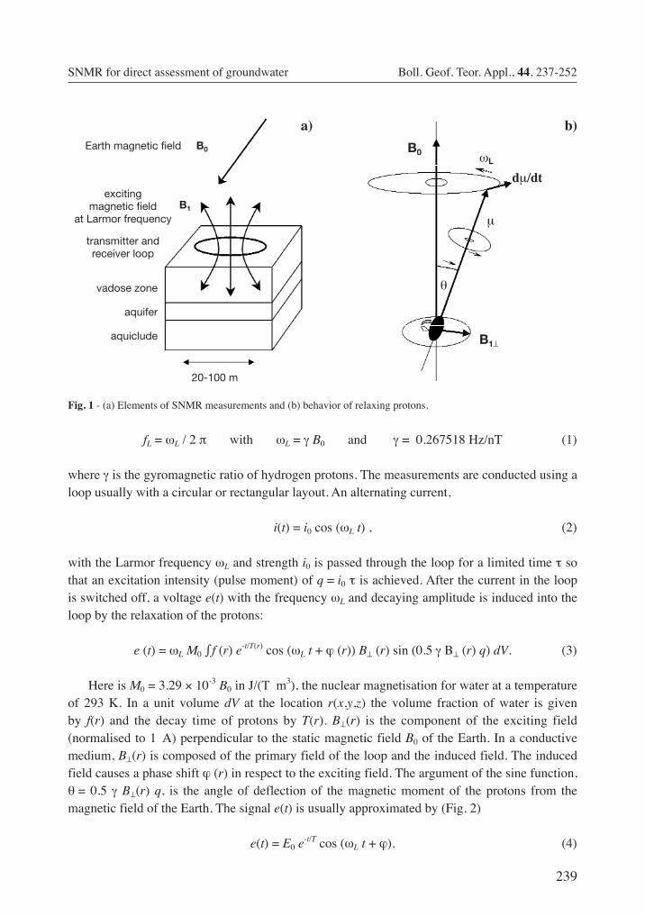
The protons of the hydrogen atoms in water molecules have a magnetic moment μ. They can be described in terms of a spinning charged particle. Generally μ is aligned to the local magnetic field B0 of the Earth. When another magnetic field B1 is applied, the axis of the spinning protons are deflected, owing to the torque applied (Fig. 1). Hereby only the component of B1 perpendicular to the static field B0 acts as the torque force. When B1 is removed, the protons generate a relaxation magnetic field as they become realigned along B0 while precessing around B0 with the Larmor frequency

239

SNMR for direct assessment of groundwater Boll. Geof. Teor. Appl., 44, 237-252

fL = ωL / 2 π with ωL = γ B0 and γ = 0.267518 Hz/nT (1)

where γ is the gyromagnetic ratio of hydrogen protons. The measurements are conducted using a loop usually with a circular or rectangular layout. An alternating current,

i(t) = i0 cos (ωL t) , (2)

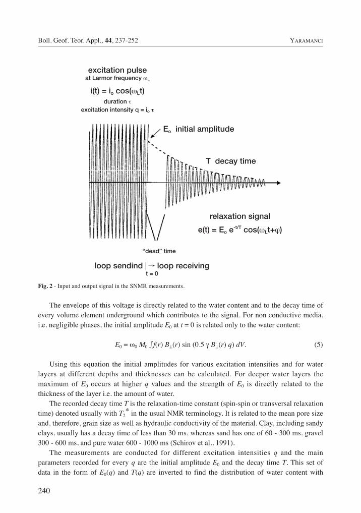
with the Larmor frequency ωL and strength i0 is passed through the loop for a limited time τ so that an excitation intensity (pulse moment) of q.=.i0 τ is achieved. After the current in the loop is switched off, a voltage e(t) with the frequency ωL and decaying amplitude is induced into the loop by the relaxation of the protons:

e (t) = ωL M0 ∫ f (r) e-t/T(r) cos (ωL t + ϕ (r)) B⊥ (r) sin (0.5 γ B⊥ (r) q) dV. (3)

Here is M0.=.3.29.×.10-3 B0 in J/(T m3), the nuclear magnetisation for water at a temperature of 293 K. In a unit volume dV at the location r(x,y,z) the volume fraction of water is given by f(r) and the decay time of protons by T(r). B⊥(r) is the component of the exciting field (normalised to 1 A) perpendicular to the static magnetic field B0 of the Earth. In a conductive medium, B⊥(r) is composed of the primary field of the loop and the induced field. The induced field causes a phase shift ϕ.(r) in respect to the exciting field. The argument of the sine function, θ.= 0.5 γ B⊥(r) q, is the angle of deflection of the magnetic moment of the protons from the magnetic field of the Earth. The signal e(t) is usually approximated by (Fig. 2)

e(t) = E0 e-t/T cos (ωL t + ϕ). (4)

Fig. 1 - (a) Elements of SNMR measurements and (b) behavior of relaxing protons.

a) b)Earth magnetic field B0

excitingmagnetic field

at Larmor frequency

transmitter andreceiver loop

vadose zone

aquifer

aquiclude

20-100 m

B1

B0

B1⊥

ωL

dμ/dt

μ

θ

240


The envelope of this voltage is directly related to the water content and to the decay time of every volume element underground which contributes to the signal. For non conductive media, i.e. negligible phases, the initial amplitude E0 at t.=.0 is related only to the water content:

E0 = ω0 M0 ∫ f(r) B⊥(r) sin (0.5 γ B⊥(r) q) dV. (5)

Using this equation the initial amplitudes for various excitation intensities and for water layers at different depths and thicknesses can be calculated. For deeper water layers the maximum of E0 occurs at higher q values and the strength of E0 is directly related to the thickness of the layer i.e. the amount of water.

The recorded decay time T is the relaxation-time constant (spin-spin or transversal relaxation time) denoted usually with T2

* in the usual NMR terminology. It is related to the mean pore size and, therefore, grain size as well as hydraulic conductivity of the material. Clay, including sandy clays, usually has a decay time of less than 30 ms, whereas sand has one of 60 - 300 ms, gravel 300 - 600 ms, and pure water 600 - 1000 ms (Schirov et al., 1991).

The measurements are conducted for different excitation intensities q and the main parameters recorded for every q are the initial amplitude E0 and the decay time T. This set of data in the form of E0(q) and T(q) are inverted to find the distribution of water content with

Fig. 2 - Input and output signal in the SNMR measurements.

excitation pulseat Larmor frequency ωL

i(t) = io cos(ωLt)duration τ

excitation intensity q = io τ

relaxation signal

e(t) = Eo e-t/T cos(ωLt+ϕ)

loop sendind → loop receivingt = 0

“dead” time

Eo initial amplitude

T decay time

241


depth f(z) and of decay time with depth T(z). Thereby, Eq. (3) is the basis of the inversion which is used in the form modified for models having horizontal layering. Two or three dimensional inversion and suitable measurement approaches for this are not available yet but are currently being investigated. The usual inversion scheme used in SNMR is based on a least square solution with a regularisation (Legchenko and Shushakov, 1998). Lately new inversion schemes are developed which use model optimisation with Simulated Annealing and allow more flexibility in designing the layer thicknesses imposed on inversion even with free layer thicknesses to be optimised (Mohnke and Yaramanci, 1999, 2002).

3. Investigations at the site Nauen

The geology of the Nauen site is quite typical of large areas in northern Germany. It is built up of Quaternary sediments which emerged in the last glacial period (Weichsel) and overlying Tertiary clays. In the actual area of investigation, these sediments consist mainly of fluvial sands bordered by glacial till. The topography is characterised by flat hills underlaid by till and plains comprising glacial fluvial sands and gravels. In the test area there is an unconfined shallow aquifer consisting of fine to medium sands underlaid by an aquiclude of marly and clayey glacial till. North of the site, the glacial till approaches the surface in a nearly E-W strike. For this reason all the main profiles were chosen N-S.

3.1. SNMR measurements

The SNMR soundings were measured at 5 locations, 25 m apart from each other, on the main profile using eight shaped loop antennas with 50 m in diameter. The antenna’s main axis was directed E-W, parallel to the strike. The simple circular or square loop, as used for an earlier single sounding, could not be used because of the high noise, generated by an electrical railway which was operating some 5 km away. The eight shaped loop allowed us to increase the signal-to-noise ratio very effectively, almost ten times compared to simple loops. Therefore, moderate stacking rates of 32 were quite sufficient. 16 to 24 different excitation intensity (q) levels were used. The frequencies have been around 2082 Hz, corresponding to the total intensity of the local Earth magnetic field of about 48900 nT, very stable within ±.0.5 Hz for all excitation intensities. Measurements were conducted with the NUMIS system (NUMIS, 1996). The processing and inversion of the data were made with the standard inversion software provided with this system (Legchenko and Shushakov, 1998).

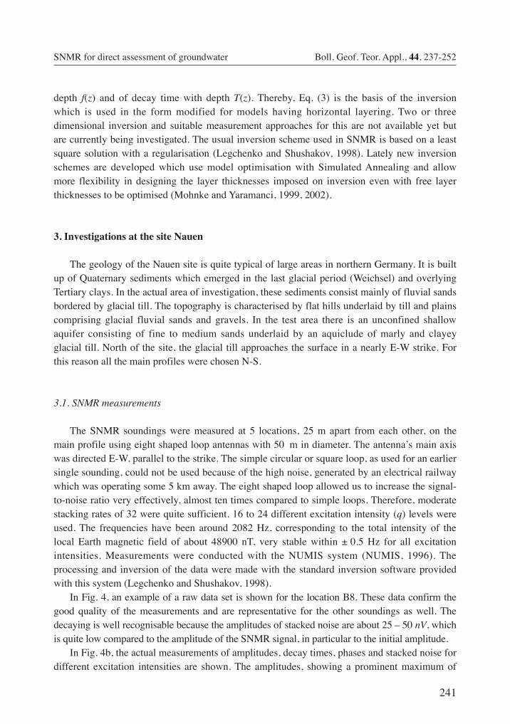
In Fig. 4, an example of a raw data set is shown for the location B8. These data confirm the good quality of the measurements and are representative for the other soundings as well. The decaying is well recognisable because the amplitudes of stacked noise are about 25.–.50 nV, which is quite low compared to the amplitude of the SNMR signal, in particular to the initial amplitude.

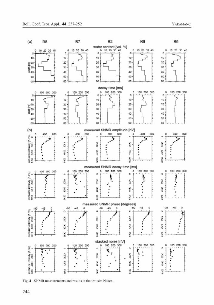
In Fig. 4b, the actual measurements of amplitudes, decay times, phases and stacked noise for different excitation intensities are shown. The amplitudes, showing a prominent maximum of

242


Fig. 3 - Example of a SNMR data set in the location B8 at the test site Nauen. Time axes are in ms. Envelopes of in-phase and out-phase components, X(t) and Y(t), are measured to yield the amplitude E(t).=.(X(t)2+Y(t)2)1/2 and phase ϕ(t).=.arctan (Y(t)/X(t)). The parameters used for the inversion are E0.=.E(t=0) and the decay time T, determined by an exponential fitting of e-t/T to E(t). The actual phase of the signal is ϕ0.=.ϕ (t=0).

243


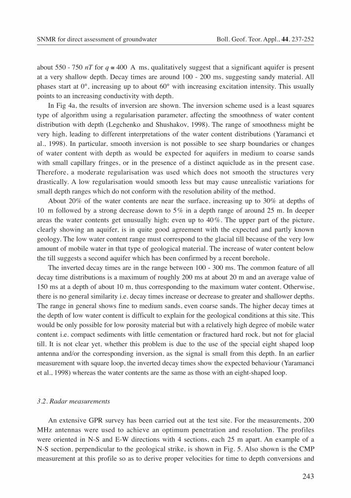
about 550.-.750 nT for q.≅.400 A ms, qualitatively suggest that a significant aquifer is present at a very shallow depth. Decay times are around 100 - 200 ms, suggesting sandy material. All phases start at 0°, increasing up to about 60° with increasing excitation intensity. This usually points to an increasing conductivity with depth.

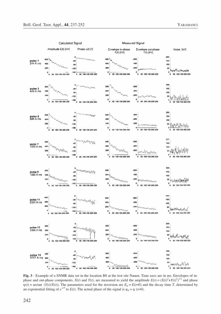
In Fig 4a, the results of inversion are shown. The inversion scheme used is a least squares type of algorithm using a regularisation parameter, affecting the smoothness of water content distribution with depth (Legchenko and Shushakov, 1998). The range of smoothness might be very high, leading to different interpretations of the water content distributions (Yaramanci et al., 1998). In particular, smooth inversion is not possible to see sharp boundaries or changes of water content with depth as would be expected for aquifers in medium to coarse sands with small capillary fringes, or in the presence of a distinct aquiclude as in the present case. Therefore, a moderate regularisation was used which does not smooth the structures very drastically. A low regularisation would smooth less but may cause unrealistic variations for small depth ranges which do not conform with the resolution ability of the method.

About 20% of the water contents are near the surface, increasing up to 30% at depths of 10 m followed by a strong decrease down to 5.% in a depth range of around 25 m. In deeper areas the water contents get unusually high; even up to 40.%. The upper part of the picture, clearly showing an aquifer, is in quite good agreement with the expected and partly known geology. The low water content range must correspond to the glacial till because of the very low amount of mobile water in that type of geological material. The increase of water content below the till suggests a second aquifer which has been confirmed by a recent borehole.

The inverted decay times are in the range between 100 - 300 ms. The common feature of all decay time distributions is a maximum of roughly 200 ms at about 20 m and an average value of 150 ms at a depth of about 10 m, thus corresponding to the maximum water content. Otherwise, there is no general similarity i.e. decay times increase or decrease to greater and shallower depths. The range in general shows fine to medium sands, even coarse sands. The higher decay times at the depth of low water content is difficult to explain for the geological conditions at this site. This would be only possible for low porosity material but with a relatively high degree of mobile water content i.e. compact sediments with little cementation or fractured hard rock, but not for glacial till. It is not clear yet, whether this problem is due to the use of the special eight shaped loop antenna and/or the corresponding inversion, as the signal is small from this depth. In an earlier measurement with square loop, the inverted decay times show the expected behaviour (Yaramanci et al., 1998) whereas the water contents are the same as those with an eight-shaped loop.

3.2. Radar measurements

An extensive GPR survey has been carried out at the test site. For the measurements, 200 MHz antennas were used to achieve an optimum penetration and resolution. The profiles were oriented in N-S and E-W directions with 4 sections, each 25 m apart. An example of a N-S section, perpendicular to the geological strike, is shown in Fig. 5. Also shown is the CMP measurement at this profile so as to derive proper velocities for time to depth conversions and

244


Fig. 4 - SNMR measurements and results at the test site Nauen.

245


rock physical considerations. The GPR can be used to map a water table by radar reflection if there is a sharp discontinuity and not a large transition zone due to the capillary fringe. Usually, the aquifer will not be penetrated properly to give reflections from its bottom due to the high absorption, i.e. energy loss in the aquifer. In Nauen, both favourable situations are met, in other words there is a sharp water table, due to the high hydraulic conductivity of the sand and therefore a good reflection and there is low electrical conductivity of water and therefore good bottom reflections, i.e. reflections from the top of the glacial till.

According to GPR measurements, the water table is at about a 2.-.3 m depth, depending on the slowly varying topography. The bottom of the aquifer, i.e. the top of glacial till, is about 15 m to the south and gradually comes up to the surface in a northern direction. North of this, below the top of till, there is no radar signal due to high absorption.

3.3. Geoelectric measurements

The clear indication of a 2-dimensional structure in GPR measurements was the reason for performing 2D-geoelectric measurement in order to get more detailed information about the resistivity structures.

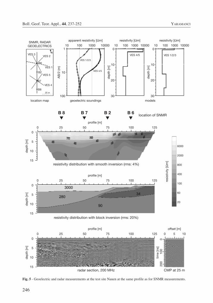
Different geoelectrical sections were measured with various lengths and electrode spacings. The result of the measurement, at the same profile as for radar measurements where a Wenner array with an electrode spacing of 2 m was used, is shown in Fig. 5. The result of a standard smooth inversion (Loke and Barker, 1996) shows well-recognisable structures of high resistivities at shallow ranges in the south, corresponding to the vadose zone, and below that, medium resistivities, corresponding to the aquifer and glacial till. To the north, these low resistivity layers come up to the surface and the values of resistivity get even lower.

Meanwhile, the classical inversion of geoelectric pseudosections, imposing a smoothness on the resistivities, has some drawbacks in the case of well-defined structures with sharp resistivity contrasts (Olayinka and Yaramanci, 2000). Not only the boundaries of the structures are blurred, but also the resistivities are far from true values. In cases like Nauen, where sharp boundaries occur, block inversion may be used (Fig. 5). With this kind of inversion, distinct resistivities are found for individual blocks, i.e. formations. The resistivities found are: 3000 Ωm for the vadose zone, 280 Ωm for the aquifer and 90 Ωm for the glacial till. These values are in very good agreement with those known from other geoelectrical surveys at Quaternary aquifers in the Berlin region. The unusually low resistivity of 34 Ωm for shallow ranges within the glacial till in the northern part of the profile shows an internal structure, probably reflecting higher clay content.

4. Estimation of water content

The water content for the aquifer indicated by SNMR is about 25-30.% (Fig. 4). That corresponds to the mobile (free) water in the pores. This is an average value for at least 3 locations to the south - B8, B7 and B2. Although the sharp boundary of water table is not well determined by the SNMR inversion used, the vadose zone with a mean water content of

246


Fig. 5 - Geoelectric and radar measurements at the test site Nauen at the same profile as for SNMR measurements.

SNMR, RADARGEOELECTRICS

location map

1

10

100

0

10

20

30

0

10

20

30geoelectric soundings models

dep

th [m

]

dep

th [m

]

AB

/2 (m

)

apparent resistivity [Ωm]

10 100 1000 10000

resistivity [Ωm]

10 100 1000 10000

resistivity [Ωm]

10 100 1000 10000

B 8▼

B 7▼

B 2▼

B 6▼

location of SNMR

profile [m]

resistivity distribution with smooth inversion (rms: 4%)

resistivity distribution with block inversion (rms: 20%)

radar section, 200 MHz CMP at 25 m

dep

th [m

]

0 25 50 75 100 125

profile [m]

resi

stiv

ity [Ω

m]

0 25 50 75 100 125

profile [m] offset [m]

0 25 50 75 100 125 0 5 10

0

5

10

15

dep

th [m

]

0

5

10

15

dep

th [m

]

0

5

10

15

time

[ns]

6000

2000

800

400

100

60

20

200

100

0

VES 3

B6

B2

B7

B8

VES 4

VES 5

VES 1

VES 2VES 1/2/3

VES 4/5

VES 4/5 VES 1/2/3

25 m

247


10- 20.% is distinguishable to some degree here. This water corresponds to the seeping water which needs some time to reach the aquifer. Below the aquifer a material with some 5-10.% water content is shown, which should be the glacial till. This, in fact, is in agreement with free water contents which can still be accommodated in the glacial till. The higher water contents found for deeper regions, suggesting a second aquifer, are confirmed by a borehole now.

4.1. Estimation of water content from radar measurements

The estimation of water content with GPR is quite straightforward and widely used (Greaves et al., 1996; Hubbard et al., 1997; Dannowski and Yaramanci, 1999). The dielectric permittivity of the rock can be determined by the velocity of electromagnetic waves measured with radar using

ε = (c/v)2 (6)

with c the velocity of electromagnetic waves in the air. To estimate water contents from radar data, the usual CRIM relation (Mavko et al., 1998) has been used. According to this formula the dielectric permittivity of the rock is related to the properties of the rock components by

√—ε = (1 – φ) √—

εm + Sφ √—εw + (1 – S) φ √—

εa (7)

with ε dielectric permittivity of rock, φ porosity, S degree of saturation, εw dielectric permittivity of water = 80, εm dielectric permittivity of matrix ≈ 4.5, εa dielectric permittivity of air = 1. The porosity is defined as φ.=.Vp/V and the degree of saturation as S.=.Vw/Vp, with V, Vp and Vw being the volumes of the rock, pores and the water respectively. The water content G.=.Vw/V is then given by

G = S φ. (8)

In the case of (full) saturation, i.e. S.=.1, Eq. (7) turns out to be

√—ε = (1 – φ) √—

εm + φ √—εw (9)

and the water content is equal to porosity, G.=.φ. The porosity determined using Eq. (9) is then used in Eq. (7), to estimate the water content in the vadose zone with the dielectric permittivity of the vadose zone.

4.2. Estimation of water content from geoelectric measurements

In order to interpret the resistivity and its local variations, the physical cause of resistivity and the influencing factors must be well understood. A model widely used for a variety of rocks is the well known Archie (1942) equation. The general model of rock conductivity σ is

248


described by two conductivities in a parallel circuit and therefore in addition (Gueguen and Palciauskas, 1994; Mavko et al., 1998)

σ = σv + σq. (10)

σv is the volume conductivity caused by the ionic conductivity of the free electrolyte in the pores and σq the capacitive interlayer conductivity due to adsorbed water at the internal surface of the pores. The conductivity σq is, in contrast to σv, strongly frequency dependent, being very small for zero frequency and becoming large with increasing frequency. For rocks with a large internal surface, for example containing a great portion of clay, σq might be very high and it is therefore called the “clay term”.

For aquifers in more sandy formations and at low frequencies σv is much larger than σq, so that σ.≅.σv. Going back to the more familiar expression in terms of resistivity, with ρ.=.1/σ, the ohmic resistivity of rock is

ρ.=.ρw φ-m S-n = F I (11)

where ρw is the resistivity of water, φ the porosity, m the Archie exponent (or cementation factor), S the degree of saturation, n the saturation exponent. The actual dependence of the resistivity on the pores is expressed with the formation factor F.=.φ-m and saturation index I.=.S-n. For a saturated rock (i.e. S.=.1) the resistivity in Eq. (11) becomes

ρo = ρw φ-m (12)

where the index o stands for (fully) saturated rock. This is the well known Archie (1942) equation, which is widely used, particularly to interpret the resistivity of well logs.

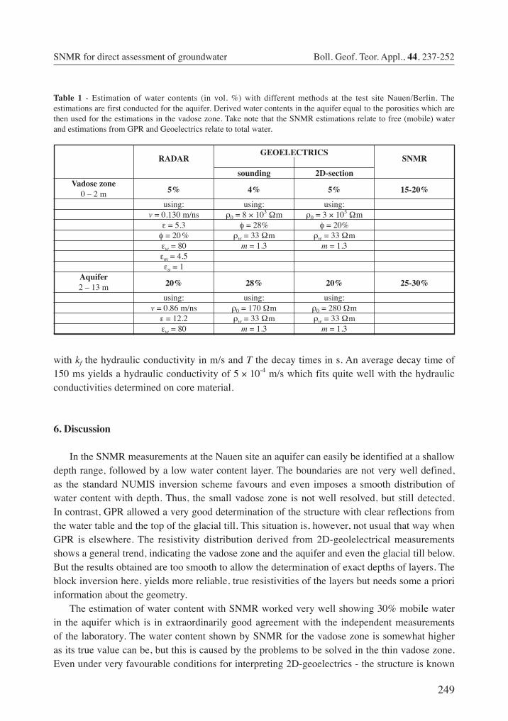
Eq. (12) is used first, to estimate the water content in the aquifer and the porosity determined hereby is then used for the estimation of porosity in the vadose zone. Very often it can be assumed that m.–.n.≅.0 and consequently Sm-n.≅.1. Even though the effect of S is not that high, but it should not be neglected a priori, particularly in cases when values for m and n are available. The parameters used for the estimation of porosity and water content at the test site Nauen and the corresponding results are shown in Table 1.

5. Estimation of hydraulic conductivities from SNMR

In order to obtain hydraulic conductivities from SNMR measurements, the empirical relationship between decay time and average grain size observed in many SNMR surveys (Schirov et al., 1991) can be used. Combining this with the relationship between grain size and hydraulic conductivity often used in hydrogeology (Hölting, 1992) leads to a simple estimation of hydraulic conductivity as proposed by Yaramanci et al., (1999):

kf ≈ T 4. (13)

249


with kf the hydraulic conductivity in m/s and T the decay times in s. An average decay time of 150 ms yields a hydraulic conductivity of 5.×.10-4 m/s which fits quite well with the hydraulic conductivities determined on core material.

6. Discussion

In the SNMR measurements at the Nauen site an aquifer can easily be identified at a shallow depth range, followed by a low water content layer. The boundaries are not very well defined, as the standard NUMIS inversion scheme favours and even imposes a smooth distribution of water content with depth. Thus, the small vadose zone is not well resolved, but still detected. In contrast, GPR allowed a very good determination of the structure with clear reflections from the water table and the top of the glacial till. This situation is, however, not usual that way when GPR is elsewhere. The resistivity distribution derived from 2D-geolelectrical measurements shows a general trend, indicating the vadose zone and the aquifer and even the glacial till below. But the results obtained are too smooth to allow the determination of exact depths of layers. The block inversion here, yields more reliable, true resistivities of the layers but needs some a priori information about the geometry.

The estimation of water content with SNMR worked very well showing 30% mobile water in the aquifer which is in extraordinarily good agreement with the independent measurements of the laboratory. The water content shown by SNMR for the vadose zone is somewhat higher as its true value can be, but this is caused by the problems to be solved in the thin vadose zone. Even under very favourable conditions for interpreting 2D-geoelectrics - the structure is known

RADAR

GEOELECTRICS SNMR

sounding 2D-section Vadose zone

5% 4% 5% 15-20%

0 – 2 m using: using: using: v = 0.130 m/ns ρ0 = 8 × 103 Ωm ρ0 = 3 × 103 Ωm ε = 5.3 φ = 28% φ = 20% φ = 20.% ρw = 33 Ωm ρw = 33 Ωm εw = 80 m = 1.3 m = 1.3 εm = 4.5 εa = 1 Aquifer

20% 28% 20% 25-30%

2 – 13 m using: using: using: v = 0.86 m/ns ρ0 = 170 Ωm ρ0 = 280 Ωm ε = 12.2 ρw = 33 Ωm ρw = 33 Ωm εw = 80 m = 1.3 m = 1.3

Table 1 - Estimation of water contents (in vol. %) with different methods at the test site Nauen/Berlin. The estimations are first conducted for the aquifer. Derived water contents in the aquifer equal to the porosities which are then used for the estimations in the vadose zone. Take note that the SNMR estimations relate to free (mobile) water and estimations from GPR and Geoelectrics relate to total water.

250


from GPR and used in geoelectric inversion, thus producing more reliable resistivities - the estimated water contents are far from reality. The result from geoelectric sounding seems good but it is not real, since the side effects probably have a large influence on it.

7. Conclusions and developments

The SNMR method has just passed the experimental stage and become a powerful tool for groundwater exploration and aquifer characterisation. Some further improvements are still necessary and currently underway. The greatest current concern is the effect of resistivities and their inclusion in the analysis and inversion. This is due to the fact that the exciting field will be modified and polarised considerably by the presence of conductive structures. Similar earlier considerations (Shushakov and Legchenko, 1992; Shushakov, 1996) led to an appropriate theoretical description and numerical handling of this problem (Valla and Legchenko, 2002; Weichmann et al., 2002). In fact, the incorporation of resistivities allows the modelling of the phases reliably (Braun et al., 2002) which is not only useful for understanding the phases measured but also the basis for a successful inversion of phases to yield the resistivity information directly from SNMR measurements.

Generally in the analysis of the SNMR the relaxation is assumed to be monoexponential. Even if individual layers were monoexponential in decaying, the integration results in a multiexponential decay in the measured signal. The most comprehensive way to take this into account to consider a decay time spectra in the data as well as in the inversion (Mohnke et al., 2001). This gives the pore size distribution which is a piece of new information and allows improved estimation of hydraulic conductivities. The estimation of water content will also be significantly improved as the initial amplitudes are much better determined using the decay spectra approach.

Currently SNMR is carried out with a 1-D working scheme. However, the errors might be very large by neglecting the 2-D or even 3-D geometry of the structures (Warsa et al., 2002) which have to be considered in the analysis and inversion in the future. Measurement layouts are to be modified to meet the multi-D conditions, which is easier to accomplish for nonconductive structures. In multi-D structures, the actual difficulty is the numerical incorporation of the electromagnetic modelling for the exciting field.

As in any geophysical measurement, the SNMR inversion also plays a key role by interpreting the data. The limits of inversion together with the imposed conditions, in terms of geometrical boundary conditions, and the differences in the basic physical model, may lead to considerable differences. The inversion of SNMR data may be ambiguous, since not only different regularisations in the inversion impose a certain degree of smoothness upon the distribution of water content (Legchenko and Shushakov, 1998; Yaramanci et al., 1998; Mohnke and Yaramanci, 1999) but also the number of layers and the size of layers forced on the inversion may considerably affect the results. The rms-error is not necessarily a sufficient measure for assessing the quality of the fit of a model to the observed data. The most recent research suggests that a layer modelling with free boundaries avoids the problems

251


associated with regularisation and takes into account the blocky character of the structure where appropriate (Mohnke and Yaramanci, 2002).

Further improvement in the inversion can be achieved for geoelectrical measurements and they can be incorporated into a joint inversion with SNMR. Examples of joint inversion of SNMR with Vertical Electrical Sounding show a considerable improvement in the detectability and geometry of the aquifers. Joint inversion allows also, the separation of mobile and adhesive water (Hertrich and Yaramanci, 2002) through appropriate petrophysical models.

At sites where no information is available in advance, SNMR should always be carried out along with geoelectrical methods, i.e. direct current geoelectric, electromagnetics and even GPR. This will help to decrease ambiguity in the results and also allow hydrogeological parameters to be estimated (Yaramanci et al., 2002). Despite all the difficulties, the quality of geophysical exploration for groundwater and aquifer properties will have an increased degree of reliability by using SNMR as a direct indicator of water and soil properties.

The importance of the SNMR method lies in its ability to detect water directly and by allowing reliable estimation of mobile water content and hydraulic conductivity. In this respect, it is unique, since all other geophysical methods yield estimates, if ever, indirectly via resistivity, induced polarisation, dielectric permittivity or seismic velocity. Using SNMR in combination with other geophysical methods not only allows direct assessment but is complementary to the information yielded by other geophysical methods.

References

Archie G.E., 1942: The electrical resistivity as an aid in determining some reservoir characteristics. Trans. Americ. Inst. Mineral. Met. and Petr. Eng. 146, 54-62.

Beauce A., Bernard J., Legchenko A. and Valla P.; 1996: Une nouvelle méthode géophysique pour les études hydrogéologiques: l’application de la résonance magnétique nucléaire. Hydrogéologie 1, 71-77.

Braun M., Hertrich M. and Yaramanci U.; 2002: Modeling of phases in Surface NMR. Proceedings of 8th European Meeting on Environmental and Engineering Geophysics, EEGS-ES.

Dannowski G. and Yaramanci U.; 1999: Estimation of water content and porosity using combined radar and geoelectrical measurements. European Journal of Environmental and Engineering Geophysics, Vol. 4, 71-85.

Goldman M., Rabinovich B., Rabinovich M., Gilad D., Gev I. and Schirov M.; 1994: Application of the integrated NMR-TDEM method in groundwater exploration in Israel. Journal of Applied Geophysics 31, 27-52.

Greaves R.J., Lesmes D.P., Lee J.M. and Toksöz M.N.; 1996: Velocity variations and water content estimated from multi-offset, ground penetrating radar. Geophysics 61, 683-695.

Gueguen Y. and Paliciauskas V.; 1994: Physics of Rocks. Princeton University Press, Princeton.

Hertrich M. and Yaramanci U.; 2002: Joint inversion of Surface Nuclear Magnetic Resonance and Vertical Electrical Sounding. Journal of Applied Geophysics 50, 179-191.

Hölting B.; 1992: Hydrogeologie. Enke Verlag, Stuttgart.

Hubbard S.S., Peterson J.E., Jr. Majer E.L., Zawislanski P.T., Wiliams K.H., Roberts J. and Wobber F.; 1997: Estimation of permeable pathways and water content using tomographic radar data. The Leading Edge 16, no. 11, 1623-1628.

Kenyon W.E.; 1992: Nuclear magnetic resonance as a petrophysical measurement. Int. Journal of Radiat. Appl. Instrum, Part E, Nuclear Geophysics 6, No. 2, 153-171.

252


Legchenko A.V., Semenov A.G. and Schirov M.D.; 1990: A device for measurement of subsurface water saturated layers parameters (in Russian). USSR Patent 1540515.

Legchenko A.V. and Shushakov O.A.; 1998: Inversion of surface NMR data. Geophysics 63, 75-84.Legchenko A.V., Shushakov O.A., Perrin J.A. and Portselan A.A.; 1995: Noninvasive NMR study of subsurface

aquifers in France. Proceedings of 65th Annual Meeting of Society of Exploration Geophysicists, 365-367.Lieblich D.A., Legchenko A., Haeni F.P. and Portselan A.A.; 1994: Surface nuclear magnetic resonance experiments

to detect subsurface water at Haddam Meadows, Connecticut. Proceedings of the Symposium on the Application of Geophysics to Engineering and Environmental Problems, Boston, 2, 717-736.

Loke M.H. and Barker R.D.; 1996: Rapid least-squares inversion of apparent resistivity pseudosections by a quasi-Newton method. Geophysical Prospecting, 44, 131-152.

Mavko G., Mukreji T. and Dvorkin J.; 1998: The Rock Physics Handbook. Cambridge University Press, Cambridge.Meju M.A., Denton P. and Fenning P.; 2002: Surface NMR sounding and inversion to detect groundwater in key

aquifers in England: comparisons with VES-TEM methods. Journal of Applied Geophysics 50, 95-111.Mohnke O. and Yaramanci U.; 1999: A new inversion scheme for surface NMR amplitudes using simulated annealing.

Proceedings of 60th Conference of European Association of Geoscientists and Engineers, 2-27.Mohnke O. and Yaramanci U.; 2002: Smooth and block inversion of surface NMR amplitudes and decay times using

simulated annealing. Journal of Applied Geophysics 50, 163-177.Mohnke O., Braun M. and Yaramanci U.; 2001: Inversion of decay time spectra from Surface-NMR data. Proceedings

of 7th European Meeting on Environmental and Engineering Geophysics, EEGS-ES.NUMIS; 1996: Manual of NUMIS system for Proton Magnetic Resonance. IRIS Instruments. Olayinka A.I. and Yaramanci U.; 2000: Use of block inversion in the 2-D interpretation of apparent resistivity data

and its comparison with smooth inversion. Journal of Applied Geophysics 45, 63-81. Schirov M., Legchenko A. and Creer G.; 1991: A new direct non-invasive groundwater detection technology for

Australia. Exploration Geophysics 22, 333-338.Semenov A.G., Burshtein A.I., Pusep A.Y. and Schirov M.D.; 1988: A device for measurement of underground

mineral parameters (in Russian). USSR Patent 1079063.Shushakov O.A.; 1996: Groundwater NMR in conductive water. Geophysics 61, 998-1006.Shushakov O.A. and Legchenko A.V.; 1992: Calculation of the proton magnetic resonance signal from groundwater

considering the electroconductivity of the medium (in Russian). Russian Acad. of Sci., Inst. of Chem. Kinetics and Combustion, Novosibirsk, issue 36, 1-26.

Supper R., Jochum B., Hübl G., Römer A. and Arndt R.; 2002: SNMR test measurements in Austria. Journal of Applied Geophysics 50, 113-121.

Valla P. and Legchenko A.; 2002: One-dimensional modelling for proton magnetic resonance sounding measurements over an electrically conductive medium. Journal of Applied Geophysics 50, 217-229.

Vouillamoz J.-M., Descloitres M., Bernard J., Fourcassier P. and Romagny L.; 2002: Application of integrated magnetic resonance sounding and resistivity methods for borehole implementation - A case study in Cambodia. Journal of Applied Geophysics 50, 67-81.

Warsa W., Mohnke O. and Yaramanci U.; 2002: 3-D modelling of Surface-NMR amplitudes and decay times. In: Water Resources and Environment Resaerch, ICWRER 2002, Eigenverlag des Forums für Abfallwirtschaft und Altlasten e.V., Dresden, 209-212.

Weichman P.B., Lun D.R., Ritzwoller M.H. and Lavely E.M.; 2002: Study of surface nuclear magnetic resonance inverse problems. Journal of Applied Geophysics 50, 129-147.

Yaramanci U., Lange G. and Knödel K.; 1998: Effects of regularisation in the inversion of Surface NMR measurements. Proceedings of 60th Conference of European Association of Geoscientists & Engineers, 10-18.

Yaramanci U., Lange G. and Hertrich M.; 2002: Aquifer characterisation using Surface NMR jointly with other geophysical techniques at the Nauen/Berlin test site. Journal of Applied Geophysics 50, 47-65.

Yaramanci U., Lange G. and Knödel K.; 1999: Surface NMR within a geophysical study of an aquifer at Haldensleben (Germany). Geophysical Prospecting 47, 923-943.

Documents

Surface Nuclear Magnetic Resonance for direct assessment ... · Surface Nuclear Magnetic Resonance for direct assessment of ... The principle of nuclear magnetic resonance, ... generate