SURGE: Continuous Detection of Bursty RegionsOver

a Stream of Spatial ObjectsKaiyu Feng1,2, Tao Guo2, Gao Cong2, Sourav S. Bhowmick2, Shuai Ma3

1 LILY, Interdisciplinary Graduate School. Nanyang Technological University, Singapore2 School of Computer Science and Engineering, Nanyang Technological University, Singapore

3 SKLSDE, Beihang University, China{kfeng002@e., tguo001@e., gaocong@, assourav@}ntu.edu.sg, mashuai@buaa.edu.cn

Abstract—With the proliferation of mobile devices andlocation-based services, continuous generation of massive volumeof streaming spatial objects (i.e., geo-tagged data) opens upnew opportunities to address real-world problems by analyzingthem. In this paper, we present a novel continuous bursty regiondetection (SURGE) problem that aims to continuously detect abursty region of a given size in a specified geographical areafrom a stream of spatial objects. Specifically, a bursty regionshows maximum spike in the number of spatial objects in agiven time window. The SURGE problem is useful in addressingseveral real-world challenges such as surge pricing problem inonline transportation and disease outbreak detection. To solvethe problem, we propose an exact solution and two approximatesolutions, and the approximation ratio is 1−α

4in terms of the

burst score, where α is a parameter to control the burst score.We further extend these solutions to support detection of top-kbursty regions. Extensive experiments with real-world data areconducted to demonstrate the efficiency and effectiveness of oursolutions.

I. INTRODUCTION

People often share geo-tagged messages through manysocial services like Twitter and Facebook. Each geo-taggeddata is associated with a timestamp, a geo-location, and a setof attributes (e.g., tweet content). In this paper, we refer tothem as spatial objects. With the proliferation of GPS-enabledmobile devices and location-based services, the amount ofsuch spatial objects (e.g., geo-tagged tweets and trip requestsusing Uber) is growing at an explosive rate. Their real-time nature coupled with multi-faceted information and rapidarrival rate in a streaming manner open up new opportunitiesto address real-world problems. For example, consider thefollowing problems.

Example 1: The world regularly faces the challenge of tack-ling a variety of virus epidemics such as SARS, MERS, Dengue,and Ebola. Most recently, the outbreak of mosquito-borneZika virus started in Brazil in 2015. Hence, the Center forDisease Control and Prevention needs to continuously monitordifferent areas for possible Zika outbreak and issue alerts topeople who are traveling to or living in regions affected byZika. Since early detection of such outbreak is paramount,how can we identify potential Zika-affected region(s) in realtime?

Fig. 1: Motivating example.

One strategy to address this issue is to continuously monitorgeo-tagged tweets (i.e., spatial objects) coming out of aspecific area (e.g., Florida) and detect regions where thereare sudden bursts in tweets related to Zika (e.g., containingZika-related keywords) in real time. Observe that these “burstyregions” are dynamic in nature. However, it is computationallychallenging to continuously monitor massive streams of spatialobjects and detect bursty regions in real time. �

Example 2: Online transportation network companies suchas Uber, Lyft, and Didi Dache have disrupted the traditionaltransportation model and have gained tremendous popularityamong consumers1. Consumers can submit a trip requestthrough their mobile apps. If a nearby driver accepts therequest, he will pickup the consumer.

Although this disruptive model has benefited many driversand consumers, the latter may have to wait for a long time fora car when the number of car requests significantly surpassesthe supply of nearby drivers. Clearly, it is beneficial to bothpassengers and drivers if we can notify idle drivers in realtime whenever there is a sudden burst in consumer demandin areas of interest to them. An additional benefit to thedrivers is that the trip fare may be increased due to the “surgepricing” policy 2 where the companies may increase a tripprice significantly when demand is high. For instance, considerFigure 1, which shows the trip requests in two time windows[t1, t2] and [t2, t3]. Suppose a driver is only interested in the

1In 2017, Uber is available in over 81 countries and 570 cities worldwide.2 For example, the price increased 10X on new year’s

eve in 2016 in the United States (www.geekwire.com/2016/customers-complain-uber-prices-surge-near-10x-new-years-eve/)

arX

iv:1

709.

0928

7v2

[cs

.DB

] 2

8 Se

p 20

17

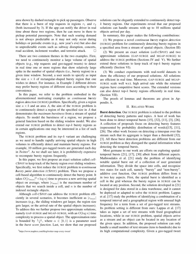
area shown by dashed rectangle to pick up passengers. Observethat there is a burst of trip requests in regions r1 and r2(both increased by 3). If the app can notify the driver in realtime about these two regions, then he can move in there topickup potential passengers. Note that such soaring demandis not always predictable as it may not only occur duringholidays or periodic events (e.g., new year’s eve) but also dueto unpredictable events such as subway disruption, concerts,road accident, inclement weather, and terrorist attack. �

There are two common themes in the two examples. First,we need to continuously monitor a large volume of spatialobjects (e.g., trip requests and geo-tagged tweets) to detectin real time one or more regions that show relatively largespike in the number of spatial objects (i.e., bursty region) in agiven time window. Second, a user needs to specify as inputthe size a × b of rectangular-shaped bursty region that onewishes to detect. For instance, in Example 2 different driversmay prefer bursty regions of different sizes according to theirconvenience.

In this paper, we refer to the problem embodied in theaforementioned motivating examples as continuous burstyregion detection (SURGE) problem. Specifically, given a regionsize a × b and an area A, the aim of the SURGE problem isto continuously detect a region of the specified size in A thatdemonstrates the maximum burstiness from a stream of spatialobjects. To model the burstiness of a region, we propose ageneral function based on the sliding window model. We alsoextend our SURGE problem to detect top-k bursty regions asin certain applications one may be interested in a list of suchregions.

The SURGE problem and its top-k variant are challengingas we need to handle rapidly arriving spatial objects in highvolumes to efficiently detect and maintain bursty regions. Forexample, 10 million geo-tagged tweets are generated each dayin Twitter3. As we shall see later, it is prohibitively expensiveto recompute bursty regions frequently.

In this paper, we first propose an exact solution called cell-CSPOT to keep track of the bursty region over sliding windows.Specifically, we first reduce the SURGE problem to continuousbursty point detection (CSPOT) problem. Then we propose acell-based algorithm to continuously detect the bursty point. Ittakes O(|cmax|2+log n) time to process a new arriving spatialobject on average, where |cmax| is the maximum number ofobjects that we search inside a cell, and n is the number ofindexed rectangle objects.

Although cell-CSPOT can address the SURGE problem effi-ciently in several scenarios, it becomes inefficient as |cmax|increases (e.g., the sliding windows get larger, the region sizegets larger, or the arrival rate of the spatial objects increases).To address this we further propose two approximate solutions,namely GAP-SURGE and MGAP-SURGE, with an O(log n) timecomplexity to process a spatial object. The approximation ratiois bounded by 1−α

4 , where α ∈ [0, 1) is a parameter usedin the burst score function. Last, we show that our proposed

3https://www.mapbox.com/blog/twitter-map-every-tweet/

solutions can be elegantly extended to continuously detect top-k bursty regions. Our experiments reveal that our proposedsolutions can handle streams with up to 10 millions spatialobjects arrived per day.

In summary, this paper makes the following contributions:(1) We propose a novel continuous bursty region detection

(SURGE) problem for continuously detecting bursty regions ina specified area from a stream of spatial objects. (Section III)

(2) We present an exact solution (cell-CSPOT) and twoapproximate solutions (GAP-SURGE and MGAP-SURGE) toaddress the SURGE problem (Sections IV and V). We furtherextend these solutions to keep track of top-k bursty regionsefficiently (Section VI).

(3) We conduct experiments with real-world datasets toshow the efficiency of our proposed solutions. All solutionsare efficient in real time. Moreover, GAP-SURGE and MGAP-SURGE scale well w.r.t. high arrival rate while the returnedregions have competitive burst scores. The extended versionscan also detect top-k bursty regions efficiently in real time.(Section VII).

The proofs of lemmas and theorems are given in Ap-pendix A.

II. RELATED WORK

Burst detection. Our SURGE problem is related to the problemof detecting bursty patterns and topics. A host of work hasbeen done to detect temporal bursts [15], [32], [11], [3], [26].A collection of proposals focus on detecting bursty features(represented by probability distribution of words)[15], [11],[26]. The other work focuses on detecting a timespan over thestream such that its aggregate is larger than a threshold [32],[3]. All these burst detection problems are different from ourSURGE problem as they disregard the spatial information whendetecting the temporal bursts.

Most germane to our work are efforts on exploring spatial-temporal bursts [21], [17], [30] albeit from different aspects.Mathioudakis et al. [21] study the problem of identifyingnotable spatial burst out of a collection of user generatedinformation. They divide the space into cells, and recognizetwo states for each cell, namely “bursty” and “non-bursty”.additive cost function. Our SURGE problem differs from itin two key aspects. First, the spatial burst is identified as acell in the grid whereas the bursty region in SURGE can belocated at any position. Second, the solution developed in [21]is designed for data stored in a data warehouse, and it cannotbe deployed or adapted to solve the SURGE problem. Lappaset al. [17] study the problem of identifying a combination of atemporal interval and a geographical region with unusual highfrequency for a term from a set of geo-tagged text streams.Its problem setting is different from ours: Lappas et al. [17]takes as input a set of text streams with fixed geographicallocations, while in our SURGE problem, spatial objects arriveas a stream and an object can be located in any location ofthe given space. In addition, the proposed solution can onlyhandle a small number of text streams (tens to hundreds) due toits high computational complexity. Given a geo-tagged tweet

stream, Zhang et al. [30] aim to continuously detect real-timelocal event. Specifically, a local event is defined as a clusterof tweets that are semantically coherent and geographicallyclose. For each keyword in a tweet, its burstiness is a linearcombination of its temporal burstiness and its spatial burstinesswith a balance parammeter η. The spatiotemporal burstinessof a cluster of tweets is the aggregation of the burstiness ofall the keywords in the cluster. Our problem differs from it inthe following aspects. First, the bursty event is identified as acluster of geo-tagged tweets, while our SURGE problem aimsto detecting a spatial region. Second, the proposed frameworkis built over geo-textual stream. The textual content serves asan important feature in their system. Our SURGE is applicableto any kind of spatial stream.

Dense region search. Our problem is also related to denseregion search over moving objects [14], [23]. Given a setof moving objects, whose positions are modeled as linearfunctions in Euclidean space, the dense region search problemaims to find all dense regions at query time t. Jensen et al.[14] constraint dense regions to be non-overlapping square-shaped regions of given size, whose density is larger than auser-specified threshold. Ni et al. [23] propose a new definitionof dense regions, which may have arbitrary shape and size. Inthe dense region search problem, the positions of the movingobjects are modeled as linear functions. Thus the positionof each moving object can be computed at any time. Incontrast, in the SURGE problem, the number of the newly-arriving spatial objects and their positions are unknown apriori. Moreover, the density function is different from ourburst score function, requiring different techniques to computethe burst score of a given region.

Region search. Our problem is also related to the regionsearch problem. A class of studies aims to find a region ofa given size such that the aggregation score of the region ismaximized[22], [7], [25], [10]. Given a set of spatial objects,the max-enclosing rectangle (MER) problem [22] aims tofind the position of a rectangle of a given size a × b suchthat the rectangle encloses the maximum number of spatialobjects. This problem is systematically investigated as themaximizing range sum (MaxRS) problem [7], [25]. Feng etal.[10] further study a generalized problem of the MaxRSproblem, in which the aggregate score function is defined bysubmodular monotone functions, which include sum. Liu etal. [19] study the problem of finding subject oriented top-khot regions, which can be considerd as a top-k version of theMaxRS problem. Cao et al.[4] study the problem of finding asubgraph of a given size with the maximum aggregation scorefrom a road network. All these aforementioned region searchproblems focus on static data. Moreover, the idea of invokingthe approach designed for the region search problem whenevera object enters or leaves the sliding windows is prohibitivelyexpensive (We will elaborate on this in Section IV-C).

Our work is closely related to the recent efforts on contin-uous MaxRS problem [2], [13]. Amagata et al. [2] proposethe problem of monitoring the MaxRS region over spatial

data streams. Specifically, given a stream of weighted spatialobjects, the continuous MaxRS problem aims to monitor thelocation of a rectangle of a size a× b such that the sum of theweights of the objects covered by the rectangle is maximized.In the proposed algorithm, a grid is imposed over the space,whose granularity is independent from the size of the queryrectangle. For each spatial object in the stream, they generate arectangle of a size a× b whose center is located at the spatialobject. The generated rectangle is mapped to the cells withwhich it overlaps. For each cell, they maintain a graph whereeach node in the graph is a rectangle mapped to this cell, andtwo nodes are connected by a directed edge if they overlapwith each other. The graph is used to handle the updates of thestream. For each rectangle in the cell, they maintain an upperbound to determine when to invoke the sweep-line algorithm[22] to find the most overlapped region inside the rectangle.With the maintained upper bounds, they use a branch-and-bound algorithm to reduce the search space. The difference ofthe SURGE problem from the continuous MaxRS problem isthat the burst score of the SURGE problem is defined over twoconsecutive sliding windows, and spatial objects in differentwindows contribute differently to the burst score. Thoughtheir solution cannot be directly applied to solve the SURGEproblem, we can adapt their solution with some modificationsfor the SURGE problem. The details of the modification arereported in Appendix J. One issue of this solution is that theyneed to maintain a graph for each cell with a space cost ofO(n2), where n is the number of rectangle objects that aremapped to the cell. When the number of objects mapped to acell is large, the space cost could be extremely high. We willshow in Section VII-B that our proposed solutions outperformthe aG2 algorithm for the SURGE problem. Hussain et al. [13]investigates the MaxRS problem on the trajectories of movingobjects. Given the trajectories of a set of moving points, theyaim to maintain the result of the MaxRS problem at any timeinstant. Its problem setting is different from ours: it takes asinput the trajectories of a set of fixed number moving objects,while in our problem, the number of spatial objects in thesliding windows may vary with time and the positions of thenew arrived objects are unknown a priori.

Data stream management. Our work is also related to datastream management. There has been a long stream of workon various aspects of data streams since the last decade.Some examples are stream clustering [1], [24], stream joinprocessing [9], and stream summarization [8]. Since most ofthese studies focus on general data streams, we only reviewthe work that involves spatial information. Given a stream ofspatial-textual objects, [28] aims to estimate the cardinality ofa spatial keyword query on objects seen so far. A host of workhas also been done to study content-based publish/subscribesystems [27], [6], [12], [18], [5], [29] over spatial objectstreams. In these systems, streaming published items aredelivered to the users with matching interests. However, noneof these studies consider the problem of detecting burstyregions.

Spatial outlier detection. Lastly, our work is also related tospatial outlier detection [20], [31], [16]. Lu et al. [20], [16] in-vestigate the spatial outlier detection problem over point data.Specifically, given a set of weighted spatial points, the spatialoutlier detection problem aims to identify top m points suchthat their weight is greatly different from the average weightof its k nearest neighbors. Zhao et al.[31] further investigateregion outliers detection over meteorological data. All theseaforementioned problems focus on static data. Moreover, theoutliers are selected from the data points in the spatial outlierdetection problem. In contrast, the location of the bursty regionin our SURGE problem can be located at any position in thespace. In addition, the spatial outlier detection problems usea totally different function to evaluate how much a data pointis different from its neighbors. Due to these differences, theirproposed solutions cannot be adapted to address the SURGEproblem.

III. PROBLEM STATEMENT

We formally define the ContinuouS BUrsty ReGionDEtection (SURGE) problem. We begin by defining someterminology.

A. Terminology

A spatial object is represented with a triple o = 〈w, ρ, tc〉,where w is the weight of o, ρ is a location point with latitudeand longitude, and tc is the creation time of object o. In thispaper, we consider a stream of spatial objects. For example,geo-tagged tweets in Twitter can be viewed as a stream ofspatial objects arriving in the order of creation time. Theweight of a tweet could be the relevance of its textual contentto a set of query keywords. The car requests in Uber can alsobe viewed as a stream of spatial objects arriving in the orderof calling time. In this case, the weight could be the passengernumber or travel fare.

We next introduce two consecutive time-based sliding win-dows, namely current and past windows. Given a window size|W |, the current window, denoted by Wc is a time periodof length |W | that stretches back to a time point t − |W |from present time t. The past window, denoted by Wp is atime period of length |W | that stretches back to a time pointt− 2|W | from the time point t− |W |.

Given a region r and a sliding window W , let O(r,W ) bethe set of spatial objects which is created in W and located inregion r, i.e., O(r,W ) = {o|o.ρ ∈ r∧o.tc ∈W}. Let f(r,W )be the summation of weights of objects in O(r,W ) normalizedby W ’s length, i.e., f(r,W ) =

∑o∈O(r,W ) o.w

|W | , which is thescore of a region r w.r.t. the sliding time window W .

Note that in this paper, for the sake of simplicity, we assumethe current window and the past window have the same length|W |. However, our proposed solution is equally applicablewhen the two sliding windows have different lengths.

B. Burst Score

Intuitively, the burst score of a region r reflects the variationin the spatial objects in r in recent period. This motivates us todesign the burst score based on the current and past windows.

We first discuss the intuition in designing the burst scoreusing Example 2. In this scenario, Uber drivers are interestedin regions in which they have a higher chance to pick upa passenger. Obviously, a driver is more likely to find apassenger in a region that contains a large number of requestsin the current window, which represents the significance of theregion. On the other hand, if a region suddenly experiences asurge of requests, which represents the burstiness of the region,then it is highly likely that existing drivers in that regionmay not be able to fulfill this sudden increase in demand.Consequently, a driver will have a higher chance to find apassenger there.

Thus, we consider the following two factors in our burstscore: (a) The score of the region w.r.t. the current window,i.e. f(r,Wc), which measures the significance, and (b) theincrease in the score of the region between the current windowand the past window, i.e., max(f(r,Wc)−f(r,Wp), 0), whichmeasures the burstiness. Note that we use the max functionto guarantee that the increase in the score between the currentand past windows is always non-negative since we are onlyinterested in increase in the score.

We now formally define the burst score as follows.Definition 1: Burst Score. Given a region r, we define its

burst score S(r) as:

S(r) = αmax(f(r,Wc)− f(r,Wp), 0) + (1− α)f(r,Wc),(1)

where α ∈ [0, 1) is a parameter that balances the significanceand the burstiness.

C. Continuous Bursty Region Detection(SURGE) Problem

We are now ready to formally define the SURGE problem.Definition 2: Continuous Bursty Region Detection

(SURGE) Problem. Consider a stream of spatial objects O.Let q = 〈A, a × b, |W |〉 be a SURGE query where A is apreferred area, a × b is the size of the query rectangle, and|W | is the length of the current and past windows. Given sucha query q, the aim of the SURGE problem is to continuouslydetect the position of the region r of size a × b in A withthe maximum burst score. The region r is referred to as thebursty region.

IV. AN EXACT SOLUTION

The SURGE problem is challenging to address due to thefollowing reasons. First, given a snapshot of the stream, weare required to locate the bursty region in the preferred areaA. Intuitively, this bursty region can be located at any pointand it is prohibitively expensive to check the region locatedat every point, which is infinite. Second, whenever a spatialobject enters or leaves the sliding windows, the burst score ofany region which encloses this object will change. This impliesthat the location of the bursty region may change as well andwe need to recompute the new bursty region. With the higharrival rate of the stream, it demands an efficient strategy toupdate the bursty region.

o1

o2

o3

g1

g2

g3p

Fig. 2: Reduce to cSPOT problem

In this section, we present a solution to address theSURGE problem. We first introduce the continuous bursty pointdetection (CSPOT) problem in Section IV-A. We show that byreducing the SURGE problem to the CSPOT problem, for anysnapshot of the stream, we convert the challenge of selectinga point from infinite points in the preferred area A to selectinga bursty point from O(n2) disjoint regions. To addressthe second challenge, we present a cell-based algorithm tocontinuously update the bursty point in Section IV-C.

A. The cSPOT Problem

We next define the CSPOT problem and present how toreduce the SURGE problem to the CSPOT problem. Firstly,we introduce some terminology that will be used to define theCSPOT problem.

Definition 3: Rectangle Object. A rectangle object, de-noted with a triple g = 〈w, ρ, tc〉, is a rectangle of size a× b,where g.w is its weight, g.ρ is the location of its left-bottomcorner, and g.tc is the creation time of g.

Given the stream of spatial objects O, each spatial object oin O can be mapped to a rectangle object g by using o as theleft-bottom corner, i.e., g.w = o.w, g.ρ = o.ρ, and g.tc = o.tc.Let G denote the stream of rectangle objects that are mappedfrom O. Let G(p,W ) be the set of rectangle objects whichcovers point p and is created in window W , i.e., G(p,W ) ={g|g.tc ∈W ∧ p ∈ g ∧ g ∈ G}.

Next, we define the burst score of a point by followingthe definition of burst score of a region in Section III . With aslight abuse of notation, we continue to use f(p,W ) and S(p)to denote the score of a point p w.r.t. the window W , and theburst score of p, respectively.

Definition 4: Burst Score of a Point. Consider a stream ofrectangle objects G. The burst score S(p) of point p is definedas

S(p) = αmax(f(p,Wc)− f(p,Wp), 0) + (1− α)f(r,Wc)

where Wc and Wp are the current and past windows, andfor a sliding window W , score f(p,W ) is the summationof weights of rectangle objects in G(p,W ), i.e., f(p,W ) =∑

g∈G(p,W ) g.w

|W | , which is the score of a point p w.r.t. the slidingtime window W .

We are now ready to formally define the CSPOT problem.Definition 5: cSPOT Problem. Consider a stream of rect-

angle objects G, a parameter α, as well as the current windowWc and past window Wp. The Continuous Bursty PointDetection (CSPOT) problem aims to keep track of a point p inthe space, such that its burst score S(p) is maximized. A pointp with the maximum score is referred to as bursty point.

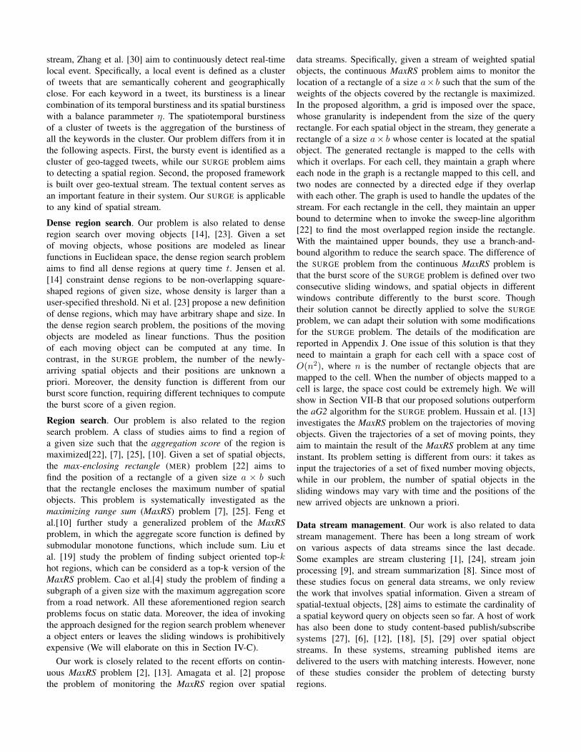
In order to reduce the SURGE problem to the CSPOTproblem, for each spatial object o in the SURGE problem, if o isin the preferred area A, i.e., o.ρ ∈ A, we generate a rectangleobject g of size a×b with o as the left-bottom corner such thato.tc = g.tc and g.ρ = o.ρ. We illustrate this reduction withthe example in Figure 2. Assume that o1, . . . , o3 are all in A.For each spatial object oi, i ∈ [1, 3], a corresponding rectangleobject gi is generated. We next show the relationship betweenthe bursty region and the bursty point of the correspondingSURGE and CSPOT problem.

Theorem 1: Let pm be a bursty point for the reduced CSPOTproblem given a snapshot. The rectangular region rm of sizea×b whose top-right corner is located at pm is a bursty regionfor the original SURGE problem for the snapshot.

Note that the reduction is inspired by the idea of trans-forming the max-enclosing rectangle problem to the rectangleintersection problem [22]. The rectangle intersection problemaims to find the most overlapped area given a set of rectangles.Since our problem has a different burst score function, thetechniques designed for the rectangle intersection problemcannot be utilized to search for the bursty point at a snapshot.

We address the SURGE problem by solving the correspond-ing CSPOT problem. Observe that in the CSPOT problem, theedges of the rectangle objects divide the space into manydisjoint regions. Consider the example in Figure 2. The shadedarea is one of the disjoint region which is the overlap of g1,g2, and g3. All points in a disjoint area are covered by thesame set of rectangles. Thus they have the same burst score.Next we present a theorem which justifies the reason behindthe reduction.

Theorem 2: Given a snapshot of the stream of rectangleobjects in the CSPOT problem, there are at most O(n2) disjointregions, where n is the number of rectangle objects in windowsWc and Wp.[22].

Since all points in a disjoint region have the same burstscore, Theorem 2 tells us that we only need to consider O(n2)disjoint regions, which addresses the first challenge of theSURGE problem, i.e., locating the bursty region from infinitepossible locations.

Example 3: Consider a snapshot of the stream shown inFigure 2. Assume that o1, o2 and o3 are three spatial objects inthe current window Wc in the SURGE problem, and oi.w = 1for i ∈ [1, 3]. According to the reduction process, g1, g2 and g3are three rectangle objects in the current window in the CSPOTproblem, and gi.w = 1 for i ∈ [1, 3]. Assume that |Wc| = 1.The shaded area is the intersection of g1, g2 and g3. Thus,any point p in the shade area has the maximum burst score,i.e., S(p) = 3. The point p in the figure is a bursty point atthe given snapshot. The solid line rectangle, whose top-rightcorner lies in p, is the bursty region as it encloses three spatialobjects and its burst score is 3. �

We next present an exact solution to address the CSPOTproblem efficiently. Specifically, given the stream of rectangleobjects, we use a grid to divide the space into cells, andmaintain the upper bounds of burst score for the points in each

Algorithm 1: SL-CSPOT AlgorithmInput: A set of rectangle objects GOutput: A bursty point p

1 p = null;2 while sweep-line meets an horizontal edge of a rectangle g do3 Ii, . . . , Ij ← the intervals covered by g;4 for interval I ∈ {Ii, . . . , Ij} do5 Update I.fc, I.fp and I.S;6 if I.S > S(p) then7 p← a point beneath I , and between the

sweep-line and next horizontal edge;8 return p;

cell. Several optimization techniques are proposed to avoidredundant recomputation. If the upper bound of any cell islarger than the score of the current bursty point, we invokea sweep-line based algorithm to search the cell to update thelocation of the bursty point.

In the rest of this section, we first introduce the sweep-line based algorithm, which finds the bursty point given aset of rectangle objects ( Section IV-B). Then we presentthe cell-based lazy update strategy, which determines whetherwe should invoke the sweep-line algorithm to recompute thebursty point (Section IV-C).

B. Detecting Bursty Point on a Snapshot

To address the first challenge, i.e., detecting the bursty pointgiven a snapshot of the stream, we propose a sweep-line basedalgorithm called SL-CSPOT in this subsection.

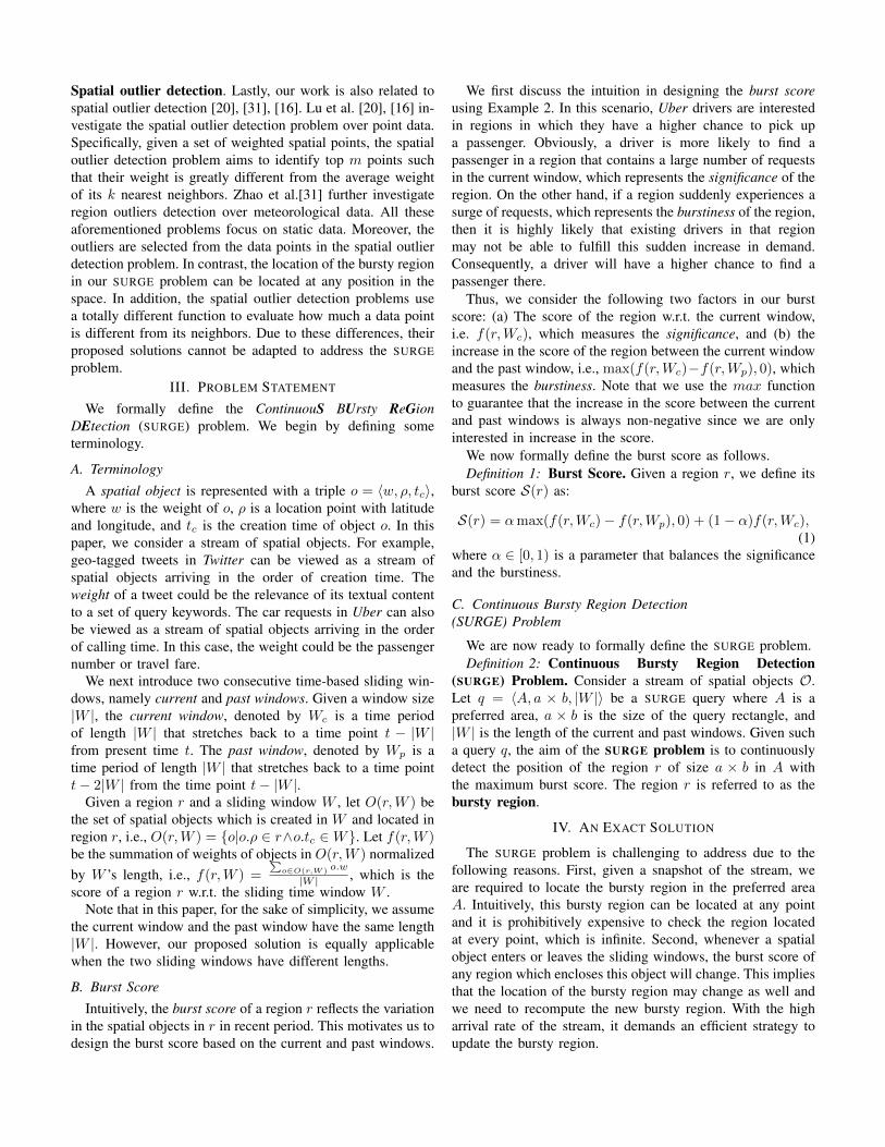
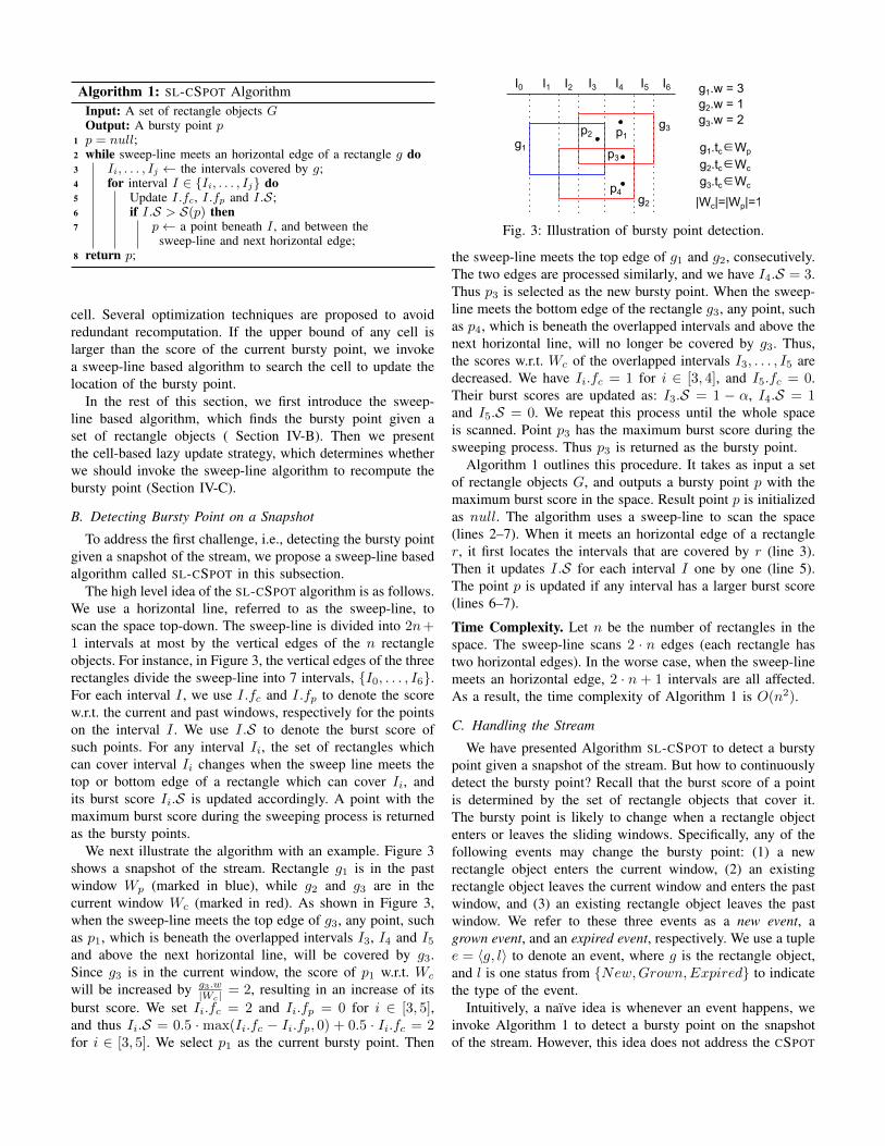
The high level idea of the SL-CSPOT algorithm is as follows.We use a horizontal line, referred to as the sweep-line, toscan the space top-down. The sweep-line is divided into 2n+1 intervals at most by the vertical edges of the n rectangleobjects. For instance, in Figure 3, the vertical edges of the threerectangles divide the sweep-line into 7 intervals, {I0, . . . , I6}.For each interval I , we use I.fc and I.fp to denote the scorew.r.t. the current and past windows, respectively for the pointson the interval I . We use I.S to denote the burst score ofsuch points. For any interval Ii, the set of rectangles whichcan cover interval Ii changes when the sweep line meets thetop or bottom edge of a rectangle which can cover Ii, andits burst score Ii.S is updated accordingly. A point with themaximum burst score during the sweeping process is returnedas the bursty points.

We next illustrate the algorithm with an example. Figure 3shows a snapshot of the stream. Rectangle g1 is in the pastwindow Wp (marked in blue), while g2 and g3 are in thecurrent window Wc (marked in red). As shown in Figure 3,when the sweep-line meets the top edge of g3, any point, suchas p1, which is beneath the overlapped intervals I3, I4 and I5and above the next horizontal line, will be covered by g3.Since g3 is in the current window, the score of p1 w.r.t. Wc

will be increased by g3.w|Wc| = 2, resulting in an increase of its

burst score. We set Ii.fc = 2 and Ii.fp = 0 for i ∈ [3, 5],and thus Ii.S = 0.5 ·max(Ii.fc − Ii.fp, 0) + 0.5 · Ii.fc = 2for i ∈ [3, 5]. We select p1 as the current bursty point. Then

g1

g2

g3

I0 I1 I2 I3 I4 I5 I6 g1.w = 3

g2.w = 1

g3.w = 2

|Wc|=|Wp|=1

p1p2

p3

p4

g1.tc∈Wp

g2.tc∈Wc

g3.tc∈Wc

Fig. 3: Illustration of bursty point detection.

the sweep-line meets the top edge of g1 and g2, consecutively.The two edges are processed similarly, and we have I4.S = 3.Thus p3 is selected as the new bursty point. When the sweep-line meets the bottom edge of the rectangle g3, any point, suchas p4, which is beneath the overlapped intervals and above thenext horizontal line, will no longer be covered by g3. Thus,the scores w.r.t. Wc of the overlapped intervals I3, . . . , I5 aredecreased. We have Ii.fc = 1 for i ∈ [3, 4], and I5.fc = 0.Their burst scores are updated as: I3.S = 1 − α, I4.S = 1and I5.S = 0. We repeat this process until the whole spaceis scanned. Point p3 has the maximum burst score during thesweeping process. Thus p3 is returned as the bursty point.

Algorithm 1 outlines this procedure. It takes as input a setof rectangle objects G, and outputs a bursty point p with themaximum burst score in the space. Result point p is initializedas null. The algorithm uses a sweep-line to scan the space(lines 2–7). When it meets an horizontal edge of a rectangler, it first locates the intervals that are covered by r (line 3).Then it updates I.S for each interval I one by one (line 5).The point p is updated if any interval has a larger burst score(lines 6–7).

Time Complexity. Let n be the number of rectangles in thespace. The sweep-line scans 2 · n edges (each rectangle hastwo horizontal edges). In the worse case, when the sweep-linemeets an horizontal edge, 2 · n + 1 intervals are all affected.As a result, the time complexity of Algorithm 1 is O(n2).

C. Handling the Stream

We have presented Algorithm SL-CSPOT to detect a burstypoint given a snapshot of the stream. But how to continuouslydetect the bursty point? Recall that the burst score of a pointis determined by the set of rectangle objects that cover it.The bursty point is likely to change when a rectangle objectenters or leaves the sliding windows. Specifically, any of thefollowing events may change the bursty point: (1) a newrectangle object enters the current window, (2) an existingrectangle object leaves the current window and enters the pastwindow, and (3) an existing rectangle object leaves the pastwindow. We refer to these three events as a new event, agrown event, and an expired event, respectively. We use a tuplee = 〈g, l〉 to denote an event, where g is the rectangle object,and l is one status from {New,Grown,Expired} to indicatethe type of the event.

Intuitively, a naı̈ve idea is whenever an event happens, weinvoke Algorithm 1 to detect a bursty point on the snapshotof the stream. However, this idea does not address the CSPOT

Algorithm 2: Cell-CSPOT AlgorithmInput: An event e = 〈g, l〉Output: A bursty point

1 Cg ← cells that are overlapped with g;2 for c ∈ Cg do3 Update U(c) using Eqn 2, 3, and status of c.p using

Lemma 4;4 c← argmaxU(c);5 while c.p is invalid do6 c.p← SL-CSPOT(c);7 Ud(c) = S(c.p);8 c← argmaxU(c);9 return c.p

problem efficiently. First, it is not necessary to search thewhole space. When an event happens, it only affects theburst score of the points inside the rectangle object of theevent. Second, frequent recomputation of the bursty point iscomputationally expensive. To address the two issues, we nextpresent a cell-based algorithm called Cell-CSPOT.

1) Cell-based Lazy Update: An event only affects the burstscores of the points inside the rectangle of the event. Thislocality property motivates us to divide the space into cells,and develop approaches to handle the cells that are affectedby an event. We first define the grid that we use as follows.

Definition 6: Grid and Cell. We consider a grid as a setof vertical and horizontal lines defined by x = i · b, y = i · afor all integers i ∈ [−∞,+∞]. For each cell c, we maintain alist of rectangle objects which overlap with the cell over thetwo sliding time windows Wc and Wp, denoted by c.G.

We have the following lemma based on obvious observa-tions.

Lemma 1: A rectangle object of size a× b overlaps with atmost four cells of the grid in Definition 6.

For each cell in the grid, we maintain a burst score upperbound for the points inside the cell (to be discussed inSection IV-C2). When an event happens, the correspondingrectangle can only affect at most four cells. Instead of search-ing the affected cells immediately after an event happens, wepropose a lazy update strategy by utilizing the maintainedupper bound: Whenever an event happens, we first updatethe upper bounds of the affected cells. Then, we invokeAlgorithm 1 to search the cells iteratively in the descendingorder of their upper bounds. In each iteration, we alwayssearch the cell with the maximum upper bound. We terminatethe process when there is no upper bound larger than thecurrent maximum burst score. Hence, when an event happens,if the upper bounds of the affected cells are less than thecurrent maximum burst score, these cells will not be searched.Thus the lazy update strategy significantly reduces the numberof times that Algorithm 1 is invoked to search affected cells.

In addition, to reuse the result of Algorithm 1 from previousiterations, we record the point returned by Algorithm 1 foreach cell which is called candidate point. The status of eachcandidate point is either valid or invalid. If the candidate pointof a cell is guaranteed to have the maximum burst score in

the cell, its status is valid. On the other hand, the status is setto invalid if it is unknown whether the candidate point has themaximum burst score. We do not need to invoke Algorithm 1to search a cell if its candidate point is valid. By exploitingthe candidate points, we can further avoid searching in somecells (discussed in SectionIV-C3).

Algorithm 2 presents an overview of our algorithm calledCell-CSPOT (cell-based CSPOT). It takes as input an event e =〈g, l〉, and reports a bursty point in the space. The algorithmfirst locates the set Cg of cells that overlap with g (line 1).Then for each cell c in Cg , it updates its upper bound basedon Equations 2, and 3 (to be introduced in Section IV-C2),and determine the status of the candidate point c.p based onLemma 4 (to be introduced in Section IV-C3) (line 3). Thenit accesses the cells in descending order of their upper boundsU(c) iteratively (lines 4–8). In each iteration, if the candidatepoint c.p is invalid, we invoke Algorithm 1 to search the celland update c.p (line 6) and the upper bound (line 7). Otherwisec.p is valid, and this indicates that c.p has the maximum burstscore in cell c and c has the maximum burst score as there is nocell whose upper bound is larger than the current maximumburst score. Therefore we terminate the process and reportpoint c.p as the result.

Time Complexity. According to Lemma 1, at most four cellsare affected by an event rectangle g. Thus, it takes O(1) timeto update the upper bounds and candidate points. A cell willnot be searched unless it is overlapped with a rectangle object.Thus, O(1) cells are searched in processing a rectangle object.In our implementation, we use a heap to maintain the cellsbased on their upper bounds. Let |cmax| be the maximumnumber of rectangle objects in a cell. Let n be the number ofrectangle objects created in Wc and Wp. It takes O(log n) timeto get the cell c and O(|cmax|2) time to search the cell. Puttingthese together, the complexity of Algorithm 2 is O(|cmax|2 +log n).Space Complexity. Each rectangle object is stored in at mostfour cells. Thus, the space cost of Algorithm 2 is O(n).

2) Upper Bound Estimation: Next, we present the detailsabout estimating the upper bound for a cell.

Static Upper Bound. We first consider a simple strategy toestimate an upper bound for a cell. According to the definitionof the burst score, rectangle objects in the current windowhave a positive impact on the burst score, while the rectangleobjects in the past window have a non-positive impact. Hence,we can estimate an upper bound burst score for a cell by onlyutilizing the objects in the current window. We refer to thisupper bound as static upper bound.

Definition 7: Static Upper Bound. For a cell c, its staticupper bound is computed as follows:

Us(c) =∑

g∈c.G∧g.tc∈Wc

g.w

|Wc|(2)

where c.G is a set of rectangle objects overlapped with c.Next, we show the correctness of the static upper bound.

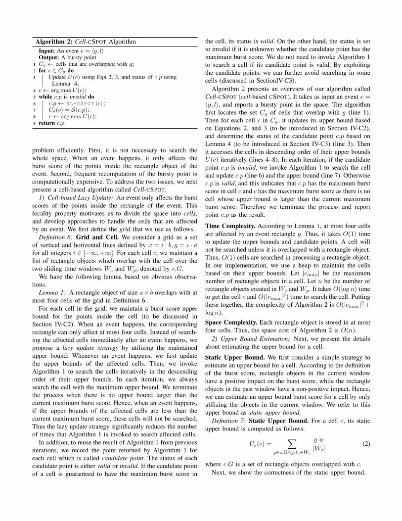
cell c

g1g2

g3

p1

Fig. 4: Cell upper bound.

Lemma 2: For any point p in a cell c, we have S(p) ≤Us(c).

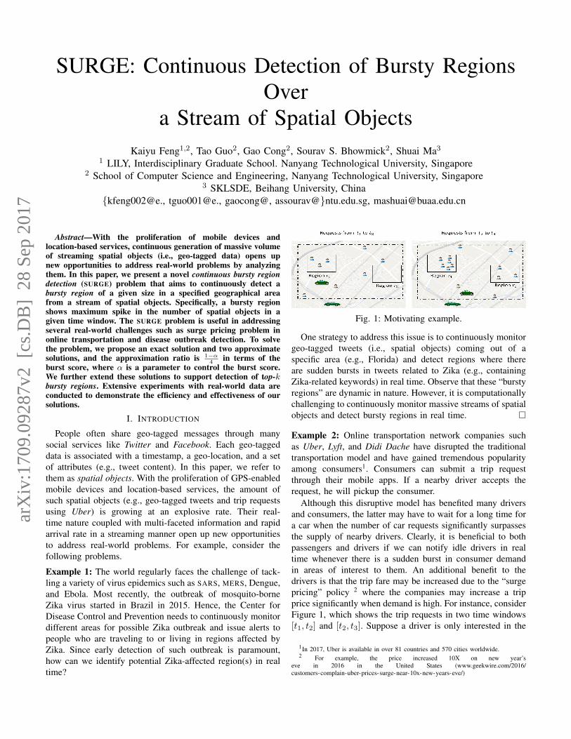
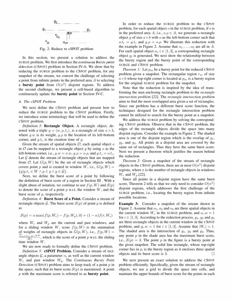
Example 4: Consider the example shown in Figure 4. Thesolid-line rectangle is a cell in the grid. After event e1 happens,there are three new rectangle objects overlapped with the cellc. The static upper bound of cell c is Us(c) = 3. �

Dynamic Upper Bound. Next, instead of just using objects inthe current window, we introduce another way to estimate theupper bound by using both the event and information from theprevious computation. Specifically, when an event happens, wedynamically update the upper bound computed from previousupper bound. We refer to such upper bound as dynamic upperbound.

Let pm be the point with the maximum burst score in cellc at a snapshot i when event ei arrives. Apparently S(pm)is an upper bound burst score for cell c at snapshot i. Thus,whenever we search a cell c with Algorithm 1 on a snapshot i,the dynamic upper bound U id(c) can be set as U id(c) = S(pm).

Let U id(c) be the upper bound of cell c on snapshot i whenevent ei arrives, and U i+1

d (c) be the upper bound when ei+1

arrives. Let g be the corresponding rectangle object of ei+1,i.e., ei+1 = 〈g, l〉. Then we have

U i+1d (c) =

U id(c) + g.w

|Wc| ei+1.l is New,

U id(c) ei+1.l is Grown,U id(c) + α g.w

|Wp| ei+1.l is Expired(3)

We next show the correctness of the dynamic upper boundwith the following lemma.

Lemma 3: Consider a cell c. For any point p in c, we haveS(p) ≤ Ud(c) after e happens.

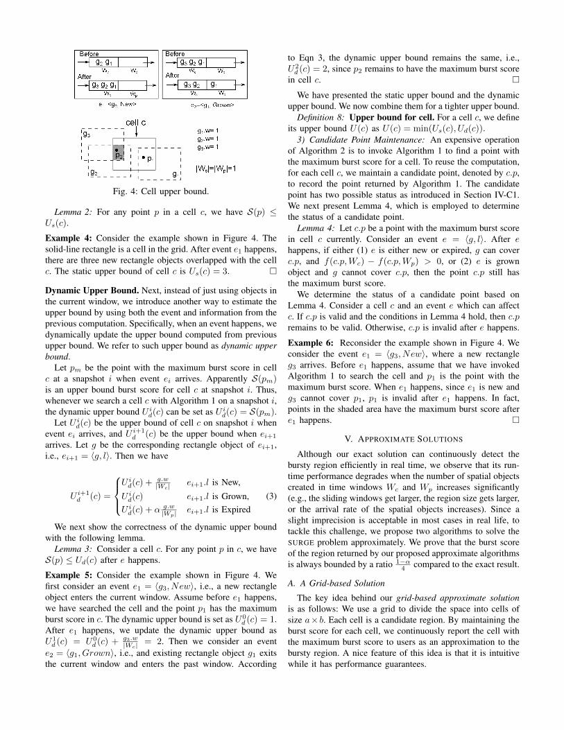
Example 5: Consider the example shown in Figure 4. Wefirst consider an event e1 = 〈g3, New〉, i.e., a new rectangleobject enters the current window. Assume before e1 happens,we have searched the cell and the point p1 has the maximumburst score in c. The dynamic upper bound is set as U0

d (c) = 1.After e1 happens, we update the dynamic upper bound asU1d (c) = U0

d (c) + g3.w|Wc| = 2. Then we consider an event

e2 = 〈g1, Grown〉, i.e., and existing rectangle object g1 exitsthe current window and enters the past window. According

to Eqn 3, the dynamic upper bound remains the same, i.e.,U2d (c) = 2, since p2 remains to have the maximum burst score

in cell c. �

We have presented the static upper bound and the dynamicupper bound. We now combine them for a tighter upper bound.

Definition 8: Upper bound for cell. For a cell c, we defineits upper bound U(c) as U(c) = min(Us(c), Ud(c)).

3) Candidate Point Maintenance: An expensive operationof Algorithm 2 is to invoke Algorithm 1 to find a point withthe maximum burst score for a cell. To reuse the computation,for each cell c, we maintain a candidate point, denoted by c.p,to record the point returned by Algorithm 1. The candidatepoint has two possible status as introduced in Section IV-C1.We next present Lemma 4, which is employed to determinethe status of a candidate point.

Lemma 4: Let c.p be a point with the maximum burst scorein cell c currently. Consider an event e = 〈g, l〉. After ehappens, if either (1) e is either new or expired, g can coverc.p, and f(c.p,Wc) − f(c.p,Wp) > 0, or (2) e is grownobject and g cannot cover c.p, then the point c.p still hasthe maximum burst score.

We determine the status of a candidate point based onLemma 4. Consider a cell c and an event e which can affectc. If c.p is valid and the conditions in Lemma 4 hold, then c.premains to be valid. Otherwise, c.p is invalid after e happens.

Example 6: Reconsider the example shown in Figure 4. Weconsider the event e1 = 〈g3, New〉, where a new rectangleg3 arrives. Before e1 happens, assume that we have invokedAlgorithm 1 to search the cell and p1 is the point with themaximum burst score. When e1 happens, since e1 is new andg3 cannot cover p1, p1 is invalid after e1 happens. In fact,points in the shaded area have the maximum burst score aftere1 happens. �

V. APPROXIMATE SOLUTIONS

Although our exact solution can continuously detect thebursty region efficiently in real time, we observe that its run-time performance degrades when the number of spatial objectscreated in time windows Wc and Wp increases significantly(e.g., the sliding windows get larger, the region size gets larger,or the arrival rate of the spatial objects increases). Since aslight imprecision is acceptable in most cases in real life, totackle this challenge, we propose two algorithms to solve theSURGE problem approximately. We prove that the burst scoreof the region returned by our proposed approximate algorithmsis always bounded by a ratio 1−α

4 compared to the exact result.

A. A Grid-based Solution

The key idea behind our grid-based approximate solutionis as follows: We use a grid to divide the space into cells ofsize a× b. Each cell is a candidate region. By maintaining theburst score for each cell, we continuously report the cell withthe maximum burst score to users as an approximation to thebursty region. A nice feature of this idea is that it is intuitivewhile it has performance guarantees.

Algorithm 3: GAP-SURGE AlgorithmInput: An event e = 〈o, l〉Output: A cell c

1 ci,j ← the cell o lies in;2 if e is new then ci,j .fc+ = o.w

|Wc| ;3 else if e is grown then ci,j .fc− = o.w

|Wc| , ci,j .fp+ = o.w|Wp| ;

4 else ci,j .fp− = o.w|Wc| ;

5 ci,j .S = max(ci,j .fc − ci,j .fp, 0) + ci.j .fc;6 c← argmax c.S;7 return c

Algorithm 3 outlines our proposed algorithm called GAP-SURGE (Grid-based APproximate SURGE). Here we abuse thenotation e = 〈o, l〉 to denote an event of spatial object o entersor leaves the sliding windows. It first locates the cell that thespatial object o lies in (line 1). The burst score of the cell c isupdated accordingly (lines 2–5). The cell with the maximumburst score is returned as an approximate result (line 6).

Before we show that the region returned by Algorithm 3has a burst score with an approximation guarantee, we presentsome interesting properties of the burst score function.

Lemma 5: For any two region r1 and r2, r1 ⊆ r2, we haveS(r2) ≥ (1− α)S(r1).

Lemma 6: Let r1, r2 be two non-overlapping regions. Wehave S(r1) + S(r2) ≥ S(r1 ∪ r2).

Now we are ready to prove the approximate ratio ofAlgorithm 3.

Theorem 3: Given a snapshot of the stream, let r be theregion returned by Algorithm 3, and ropt be the bursty regionreturned by our exact solution. We have S(r) ≥ 1−α

4 S(ropt).Lemma 7: The approximation ratio is tight.

Time Complexity. In Algorithm 3, it takes constant time tolocate the cell and update the burst score. In our implemen-tation, we use a heap to maintain all cells according to theirburst scores. Let n be the number of spatial objects created inWc and Wp. Since there are O(n) non-empty cells, it takesO(log n) time to report the cell with the maximum burst score.

B. A Multi-Grid-Based Solution

The burst score of the region returned by Algorithm 3 ishighly dependent on the position of the grid. In this subsection,we adopt multiple grids to further improve the result quality.

In the grid-based solution, we use a grid defined by lines

Grid 1: x = i · b, y = i · a

for all integers i ∈ [−∞,+∞]. By shifting the grid, wegenerate three additional grids for all integers i ∈ [−∞,+∞]:

Grid 2: x = 0.5b+ i · b, y = i · a,Grid 3: x = b+ i · b, y = 0.5a+ i · a,Grid 4: x = 0.5b+ i · b, y = 0.5a+ i · a,

The multi-grid-based solution (called the MGAP-SURGEalgorithm) invokes Algorithm 3 four times by using the fourdifferent grids. Among the four returned regions, the one withthe maximum burst score is returned to users. The pseudocode

of the MGAP-SURGE algorithm is reported in Algorithm 5 inAppendix I.

Theorem 4: The approximate ratio of the MGAP-SURGEalgorithm is 1−α

4 .Time Complexity. MGAP-SURGE invokes Algorithm 3 fourtimes, and its complexity is O(log n), where n is the numberof spatial objects created in Wc and Wp.

VI. TOP-K BURSTY REGION DETECTION

Recall that in Example 1, it is paramount to monitor regionswith outbreak of diseases. Intuitively, monitoring only the mostbursty region is not sufficient. In fact, it is reasonable to beinterested in a small list of such bursty regions. Specifically,given the size of a region, we need to continuously monitorthe top-k regions of the given size with highest burst scores.In this section, we present how we can elegantly extend ourproposed solutions to continuously detect top-k regions withhighest burst scores. We begin by formally defining the top-kbursty regions.

A. Definition

Although at first glance it may seem that it is easy to definetop-k bursty regions, in reality it is tricky. First of all, are thetop-k regions allowed to overlap? It may seem that detectingk non-overlapping regions is a good choice. However, thenon-overlapping requirement may lead us to overlooking somehighly bursty regions. Hence, it is beneficial to allow the top-kbursty regions to be overlapping instead of disjoint in nature.

Next, how do we define the burst scores for two overlappedregions? For example, if a spatial object lies at the intersectionof two overlapping regions, which region’s burst score shouldit contribute to? A naı̈ve idea is to consider it in both regions.However, this may result in k regions that are highly similarto one another. To resolve this issue, we ensure that a spatialobject contributes only to the burst score of at most one region.

The aforementioned considerations lead us to a greedystrategy for defining the top-k bursty regions. Specifically,given the first i bursty regions, the (i+1)-th bursty region is theregion with maximum burst score in the space but excludingall spatial objects that are already covered by the first i burstyregions.

Definition 9: Top-k Bursty Regions. Given k rectangularregions r1, . . . , rk such that each has a size of a× b, we sayr1, . . . , rk are the top-k bursty regions if and only if for anyregion r of size a×b, we have S(ri\r[1,i−1]) ≥ S(r\r[1,i−1])for i ∈ [1, k], where r[1,i−1] is union of regions r1, . . . , ri−1.

In order to address the top-k bursty regions problem, wereduce the top-k bursty regions problem to k CSPOT problemsfollowing the reduction in Section IV-A. The (i+1)-th CSPOTproblem aims to detect the (i + 1)-th bursty point from thespace that excludes the set of rectangles that cover the top-ibursty points.

Observe that Definition 9 essentially paves the way to agreedy approach for selecting top-k bursty regions. Wheneveran event happens, we can first detect a region with themaximum burst score by invoking Algorithm 1. Then we

remove the spatial objects covered by the region. After that,we detect a region with the maximum burst score over theremaining objects. We repeat this process until k regions areselected.

However, the naı̈ve strategy is inefficient as there are toomany redundant computations, i.e., it is possible that we searcha cell in all the k reduced CSPOT problems. To address thek CSPOT problems efficiently, we want to share the commoncomputations among the k CSPOT problems.

B. Extension of the Exact Solution

In the extension of our exact solution, for each cell c, wemaintain k upper bounds and k candidate points in orderto solve the k CSPOT problems by following the idea ofAlgorithm 2. For each CSPOT problem, we adopt the lazyupdate strategy to access the cells in descending order of theirupper bounds. If the candidate point of the top cell is not valid,we search the cell by invoking Algorithm 1.

We develop two ideas of sharing computation among thek CSPOT problems. Firstly, if a rectangle object can coverthe i-th bursty point, it will not be considered in the CSPOTproblems with order higher than i. For the extension, wemaintain a level, denoted by g.lvl, for each rectangle objectg. To select the i-th bursty point in response to a new event,we consider the set of rectangles G[i : k] whose levels are nosmaller than i, i.e., G[i : k] = {g|g.lvl ≥ i}. When the i-thbursty point is selected, the levels of all the rectangles thatcover the i-th bursty point are set as i, and these rectangleswill not be considered by the CSPOT problems with a higherorder than i. Meanwhile, if a rectangle covers the old i-thbursty point, but not the new i-th point, its level is reset to kso that it will be considered in all the k CSPOT problems.

Secondly, if no rectangle in a cell covers any of the kdetected bursty points, all the rectangles in the cell will beconsidered in all k CSPOT problems. Thus, the upper boundsand the candidate points w.r.t. the k CSPOT problems forthe cell are the same. That is, once the upper bound andthe candidate point for the cell are computed for one CSPOTproblem, we do not need to recompute them again for otherCSPOT problems.

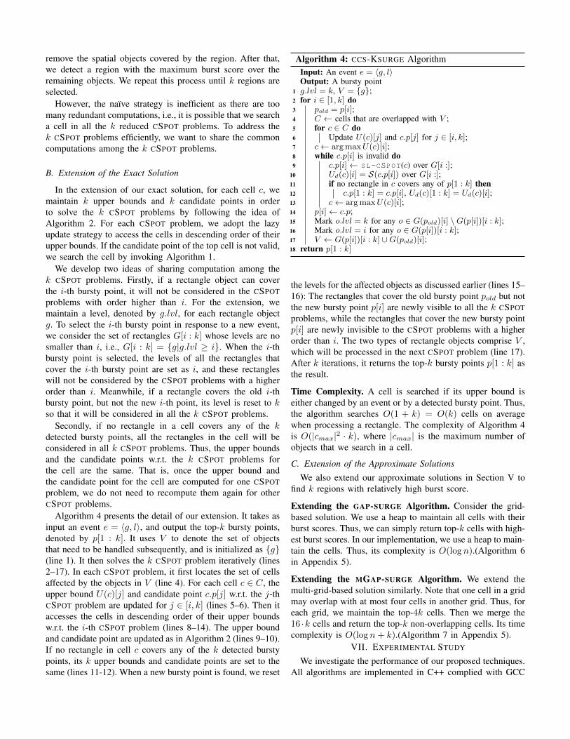
Algorithm 4 presents the detail of our extension. It takes asinput an event e = 〈g, l〉, and output the top-k bursty points,denoted by p[1 : k]. It uses V to denote the set of objectsthat need to be handled subsequently, and is initialized as {g}(line 1). It then solves the k CSPOT problem iteratively (lines2–17). In each CSPOT problem, it first locates the set of cellsaffected by the objects in V (line 4). For each cell c ∈ C, theupper bound U(c)[j] and candidate point c.p[j] w.r.t. the j-thCSPOT problem are updated for j ∈ [i, k] (lines 5–6). Then itaccesses the cells in descending order of their upper boundsw.r.t. the i-th CSPOT problem (lines 8–14). The upper boundand candidate point are updated as in Algorithm 2 (lines 9–10).If no rectangle in cell c covers any of the k detected burstypoints, its k upper bounds and candidate points are set to thesame (lines 11-12). When a new bursty point is found, we reset

Algorithm 4: CCS-KSURGE AlgorithmInput: An event e = 〈g, l〉Output: A bursty point

1 g.lvl = k, V = {g};2 for i ∈ [1, k] do3 pold = p[i];4 C ← cells that are overlapped with V ;5 for c ∈ C do6 Update U(c)[j] and c.p[j] for j ∈ [i, k];7 c← argmaxU(c)[i];8 while c.p[i] is invalid do9 c.p[i]← SL-CSPOT(c) over G[i :];

10 Ud(c)[i] = S(c.p[i]) over G[i :];11 if no rectangle in c covers any of p[1 : k] then12 c.p[1 : k] = c.p[i], Ud(c)[1 : k] = Ud(c)[i];13 c← argmaxU(c)[i];14 p[i]← c.p;15 Mark o.lvl = k for any o ∈ G(pold)[i] \G(p[i])[i : k];16 Mark o.lvl = i for any o ∈ G(p[i])[i : k];17 V ← G(p[i])[i : k] ∪G(pold)[i];18 return p[1 : k]

the levels for the affected objects as discussed earlier (lines 15–16): The rectangles that cover the old bursty point pold but notthe new bursty point p[i] are newly visible to all the k CSPOTproblems, while the rectangles that cover the new bursty pointp[i] are newly invisible to the CSPOT problems with a higherorder than i. The two types of rectangle objects comprise V ,which will be processed in the next CSPOT problem (line 17).After k iterations, it returns the top-k bursty points p[1 : k] asthe result.

Time Complexity. A cell is searched if its upper bound iseither changed by an event or by a detected bursty point. Thus,the algorithm searches O(1 + k) = O(k) cells on averagewhen processing a rectangle. The complexity of Algorithm 4is O(|cmax|2 · k), where |cmax| is the maximum number ofobjects that we search in a cell.

C. Extension of the Approximate Solutions

We also extend our approximate solutions in Section V tofind k regions with relatively high burst score.

Extending the GAP-SURGE Algorithm. Consider the grid-based solution. We use a heap to maintain all cells with theirburst scores. Thus, we can simply return top-k cells with high-est burst scores. In our implementation, we use a heap to main-tain the cells. Thus, its complexity is O(log n).(Algorithm 6in Appendix 5).

Extending the MGAP-SURGE Algorithm. We extend themulti-grid-based solution similarly. Note that one cell in a gridmay overlap with at most four cells in another grid. Thus, foreach grid, we maintain the top-4k cells. Then we merge the16 ·k cells and return the top-k non-overlapping cells. Its timecomplexity is O(log n+ k).(Algorithm 7 in Appendix 5).

VII. EXPERIMENTAL STUDY

We investigate the performance of our proposed techniques.All algorithms are implemented in C++ complied with GCC

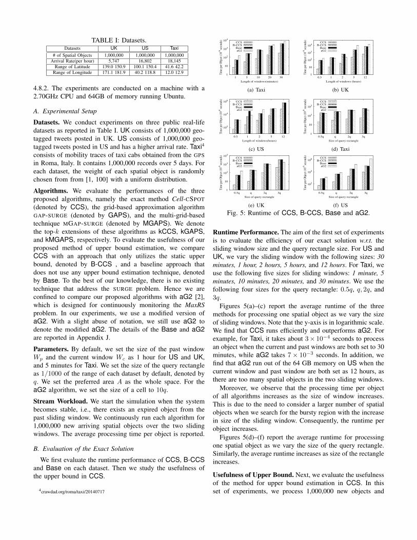
TABLE I: Datasets.Datasets UK US Taxi

# of Spatial Objects 1,000,000 1,000,000 1,000,000Arrival Rate(per hour) 5,747 16,802 18,145

Range of Latitude 139.0 150.9 100.1 150.4 41.6 42.2Range of Longitude 171.1 181.9 40.2 118.8 12.0 12.9

4.8.2. The experiments are conducted on a machine with a2.70GHz CPU and 64GB of memory running Ubuntu.

A. Experimental Setup

Datasets. We conduct experiments on three public real-lifedatasets as reported in Table I. UK consists of 1,000,000 geo-tagged tweets posted in UK. US consists of 1,000,000 geo-tagged tweets posted in US and has a higher arrival rate. Taxi4

consists of mobility traces of taxi cabs obtained from the GPSin Roma, Italy. It contains 1,000,000 records over 5 days. Foreach dataset, the weight of each spatial object is randomlychosen from from [1, 100] with a uniform distribution.

Algorithms. We evaluate the performances of the threeproposed algorithms, namely the exact method Cell-CSPOT(denoted by CCS), the grid-based approximation algorithmGAP-SURGE (denoted by GAPS), and the multi-grid-basedtechnique MGAP-SURGE (denoted by MGAPS). We denotethe top-k extensions of these algorithms as kCCS, kGAPS,and kMGAPS, respectively. To evaluate the usefulness of ourproposed method of upper bound estimation, we compareCCS with an approach that only utilizes the static upperbound, denoted by B-CCS , and a baseline approach thatdoes not use any upper bound estimation technique, denotedby Base. To the best of our knowledge, there is no existingtechnique that address the SURGE problem. Hence we areconfined to compare our proposed algorithms with aG2 [2],which is designed for continuously monitoring the MaxRSproblem. In our experiments, we use a modified version ofaG2. With a slight abuse of notation, we still use aG2 todenote the modified aG2. The details of the Base and aG2are reported in Appendix J.

Parameters. By default, we set the size of the past windowWp and the current window Wc as 1 hour for US and UK,and 5 minutes for Taxi. We set the size of the query rectangleas 1/1000 of the range of each dataset by default, denoted byq. We set the preferred area A as the whole space. For theaG2 algorithm, we set the size of a cell to 10q.

Stream Workload. We start the simulation when the systembecomes stable, i.e., there exists an expired object from thepast sliding window. We continuously run each algorithm for1,000,000 new arriving spatial objects over the two slidingwindows. The average processing time per object is reported.

B. Evaluation of the Exact Solution

We first evaluate the runtime performance of CCS, B-CCSand Base on each dataset. Then we study the usefulness ofthe upper bound in CCS.

4crawdad.org/roma/taxi/20140717

1

10

102

103

104

1 5 10 20 30

Tim

e pe

r O

bjec

t (1

0-6 s

econ

ds)

Length of windows(minutes)

CCSB-CCS

BaseaG2

(a) Taxi

1

10

102

103

104

0.5 1 2 5 12

Tim

e pe

r O

bjec

t (1

0-6 s

econ

ds)

Length of windows (hours)

CCSB-CCS

BaseaG2

(b) UK

102

104

106

0.5 1 2 5 12

Tim

e pe

r O

bjec

t (1

0-6 s

econ

ds)

Length of windows(hours)

CCSB-CCS

BaseaG2

(c) US

1

10

102

103

0.5q q 2q 3q

Tim

e pe

r O

bjec

t (1

0-6 s

econ

ds)

Size of query rectangle

CCSB-CCS

BaseaG2

(d) Taxi

1

10

102

103

104

0.5q q 2q 3q

Tim

e pe

r O

bjec

t (1

0-6 s

econ

ds)

Size of query rectangle

CCSB-CCS

BaseaG2

(e) UK

102

104

106

0.5q q 2q 3q

Tim

e pe

r O

bjec

t (1

0-6 s

econ

ds)

Size of query rectangle

CCSB-CCS

BaseaG2

(f) USFig. 5: Runtime of CCS, B-CCS, Base and aG2.

Runtime Performance. The aim of the first set of experimentsis to evaluate the efficiency of our exact solution w.r.t. thesliding window size and the query rectangle size. For US andUK, we vary the sliding window with the following sizes: 30minutes, 1 hour, 2 hours, 5 hours, and 12 hours. For Taxi, weuse the following five sizes for sliding windows: 1 minute, 5minutes, 10 minutes, 20 minutes, and 30 minutes. We use thefollowing four sizes for the query rectangle: 0.5q, q, 2q, and3q.

Figures 5(a)–(c) report the average runtime of the threemethods for processing one spatial object as we vary the sizeof sliding windows. Note that the y-axis is in logarithmic scale.We find that CCS runs efficiently and outperforms aG2. Forexample, for Taxi, it takes about 3× 10−4 seconds to processan object when the current and past windows are both set to 30minutes, while aG2 takes 7× 10−3 seconds. In addition, wefind that aG2 run out of the 64 GB memory on US when thecurrent window and past window are both set as 12 hours, asthere are too many spatial objects in the two sliding windows.

Moreover, we observe that the processing time per objectof all algorithms increases as the size of window increases.This is due to the need to consider a larger number of spatialobjects when we search for the bursty region with the increasein size of the sliding window. Consequently, the runtime perobject increases.

Figures 5(d)–(f) report the average runtime for processingone spatial object as we vary the size of the query rectangle.Similarly, the average runtime increases as size of the rectangleincreases.

Usefulness of Upper Bound. Next, we evaluate the usefulnessof the method for upper bound estimation in CCS. In thisset of experiments, we process 1,000,000 new objects and

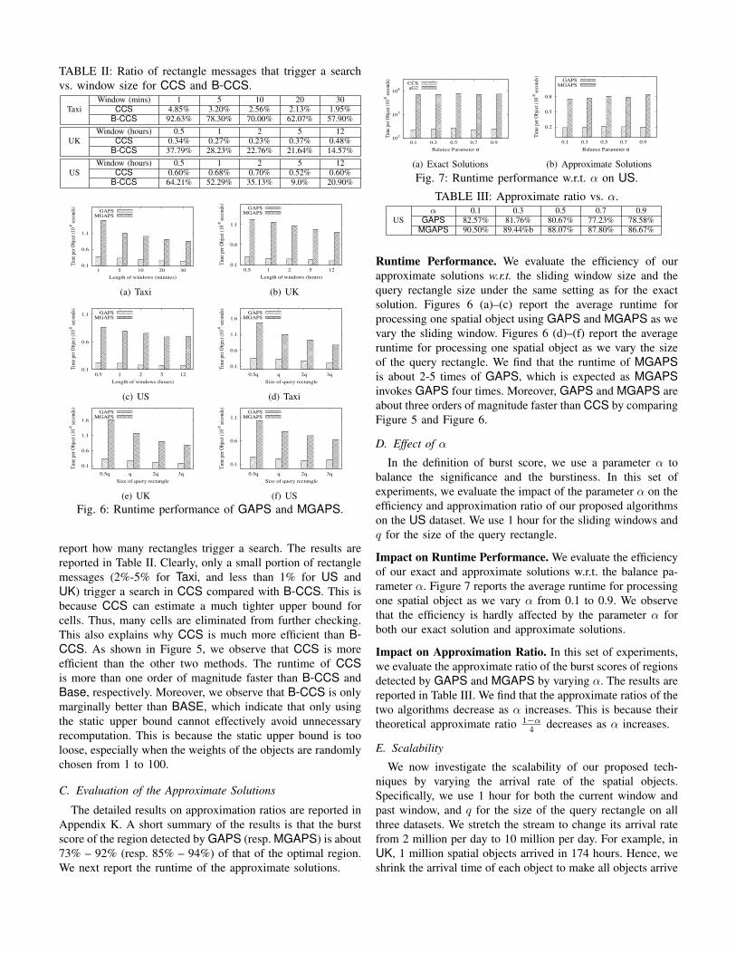
TABLE II: Ratio of rectangle messages that trigger a searchvs. window size for CCS and B-CCS.

TaxiWindow (mins) 1 5 10 20 30

CCS 4.85% 3.20% 2.56% 2.13% 1.95%B-CCS 92.63% 78.30% 70.00% 62.07% 57.90%

UKWindow (hours) 0.5 1 2 5 12

CCS 0.34% 0.27% 0.23% 0.37% 0.48%B-CCS 37.79% 28.23% 22.76% 21.64% 14.57%

USWindow (hours) 0.5 1 2 5 12

CCS 0.60% 0.68% 0.70% 0.52% 0.60%B-CCS 64.21% 52.29% 35.13% 9.0% 20.90%

0.1

0.6

1.1

1 5 10 20 30

Tim

e pe

r O

bjec

t (10

-6 s

econ

ds)

Length of windows (minutes)

GAPSMGAPS

(a) Taxi

0.1

0.6

1.1

0.5 1 2 5 12

Tim

e pe

r O

bjec

t (1

0-6 s

econ

ds)

Length of windows (hours)

GAPSMGAPS

(b) UK

0.1

0.6

1.1

0.5 1 2 5 12

Tim

e pe

r O

bjec

t (1

0-6 s

econ

ds)

Length of windows (hours)

GAPSMGAPS

(c) US

0.1

0.6

1.1

1.6

0.5q q 2q 3q

Tim

e pe

r O

bjec

t (1

0-6 s

econ

ds)

Size of query rectangle

GAPSMGAPS

(d) Taxi

0.1

0.6

1.1

1.6

0.5q q 2q 3q

Tim

e pe

r O

bjec

t (1

0-6 s

econ

ds)

Size of query rectangle

GAPSMGAPS

(e) UK

0.1

0.6

1.1

0.5q q 2q 3q

Tim

e pe

r O

bjec

t (1

0-6 s

econ

ds)

Size of query rectangle

GAPSMGAPS

(f) USFig. 6: Runtime performance of GAPS and MGAPS.

report how many rectangles trigger a search. The results arereported in Table II. Clearly, only a small portion of rectanglemessages (2%-5% for Taxi, and less than 1% for US andUK) trigger a search in CCS compared with B-CCS. This isbecause CCS can estimate a much tighter upper bound forcells. Thus, many cells are eliminated from further checking.This also explains why CCS is much more efficient than B-CCS. As shown in Figure 5, we observe that CCS is moreefficient than the other two methods. The runtime of CCSis more than one order of magnitude faster than B-CCS andBase, respectively. Moreover, we observe that B-CCS is onlymarginally better than BASE, which indicate that only usingthe static upper bound cannot effectively avoid unnecessaryrecomputation. This is because the static upper bound is tooloose, especially when the weights of the objects are randomlychosen from 1 to 100.

C. Evaluation of the Approximate Solutions

The detailed results on approximation ratios are reported inAppendix K. A short summary of the results is that the burstscore of the region detected by GAPS (resp. MGAPS) is about73% – 92% (resp. 85% – 94%) of that of the optimal region.We next report the runtime of the approximate solutions.

102

103

104

0.1 0.3 0.5 0.7 0.9

Tim

e pe

r O

bjec

t (10

-6 s

econ

ds)

Balance Parameter α

CCSaG2

(a) Exact Solutions

0.2

0.5

0.8

0.1 0.3 0.5 0.7 0.9

Tim

e pe

r O

bjec

t (1

0-6 s

econ

ds)

Balance Parameter α

GAPSMGAPS

(b) Approximate Solutions

Fig. 7: Runtime performance w.r.t. α on US.

TABLE III: Approximate ratio vs. α.

USα 0.1 0.3 0.5 0.7 0.9

GAPS 82.57% 81.76% 80.67% 77.23% 78.58%MGAPS 90.50% 89.44%b 88.07% 87.80% 86.67%

Runtime Performance. We evaluate the efficiency of ourapproximate solutions w.r.t. the sliding window size and thequery rectangle size under the same setting as for the exactsolution. Figures 6 (a)–(c) report the average runtime forprocessing one spatial object using GAPS and MGAPS as wevary the sliding window. Figures 6 (d)–(f) report the averageruntime for processing one spatial object as we vary the sizeof the query rectangle. We find that the runtime of MGAPSis about 2-5 times of GAPS, which is expected as MGAPSinvokes GAPS four times. Moreover, GAPS and MGAPS areabout three orders of magnitude faster than CCS by comparingFigure 5 and Figure 6.

D. Effect of α

In the definition of burst score, we use a parameter α tobalance the significance and the burstiness. In this set ofexperiments, we evaluate the impact of the parameter α on theefficiency and approximation ratio of our proposed algorithmson the US dataset. We use 1 hour for the sliding windows andq for the size of the query rectangle.

Impact on Runtime Performance. We evaluate the efficiencyof our exact and approximate solutions w.r.t. the balance pa-rameter α. Figure 7 reports the average runtime for processingone spatial object as we vary α from 0.1 to 0.9. We observethat the efficiency is hardly affected by the parameter α forboth our exact solution and approximate solutions.

Impact on Approximation Ratio. In this set of experiments,we evaluate the approximate ratio of the burst scores of regionsdetected by GAPS and MGAPS by varying α. The results arereported in Table III. We find that the approximate ratios of thetwo algorithms decrease as α increases. This is because theirtheoretical approximate ratio 1−α

4 decreases as α increases.

E. Scalability

We now investigate the scalability of our proposed tech-niques by varying the arrival rate of the spatial objects.Specifically, we use 1 hour for both the current window andpast window, and q for the size of the query rectangle on allthree datasets. We stretch the stream to change its arrival ratefrom 2 million per day to 10 million per day. For example, inUK, 1 million spatial objects arrived in 174 hours. Hence, weshrink the arrival time of each object to make all objects arrive

102

103

104

105

2 4 6 8 10

Run

tim

e fo

r pr

oces

sing

(se

cond

s)

Arrival Rate (million per day)

UKUS

Taxi

(a) CCS

0.1

0.2

0.3

2 4 6 8 10

Run

tim

e fo

r pr

oces

sing

(se

cond

s)

Arrival Rate (million per day)

TaxiUSUK

(b) GAPSFig. 8: Scalability study.

10-1

10

103

105

5 10 20 30 60

Tim

e pe

r O

bjec

t (1

0-6 s

econ

ds)

Length of Sliding Window (Minute)

kGAPSkMGAPS

kCCS

(a) Taxi

10-1

10

103

105

0.5 1 2 12 24

Tim

e pe

r O

bjec

t (1

0-6 s

econ

ds)

Length of Sliding Window (Hours)

kGAPSkMGAPS

kCCS

(b) UK

10-1

10

103

105

0.5 1 2 12 24

Tim

e pe

r O

bjec

t (1

0-6 s

econ

ds)

Length of Sliding Window (Hours)

kGAPSkMGAPS

kCCSNaive

(c) US

10

40

70

100

3 5 7 9

Tim

e pe

r O

bjec

t (1

0-3se

cond

s)

k

UKTaxi

US

(d) kCCS

0.4

0.5

0.6

3 5 7 9

Tim

e pe

r O

bjec

t (1

0-6se

cond

s)

k

USTaxiUK

(e) kGAPS

10

20

30

40

3 5 7 9

Tim

e pe

r O

bjec

t (1

0-6se

cond

s)

k

USUK

Taxi

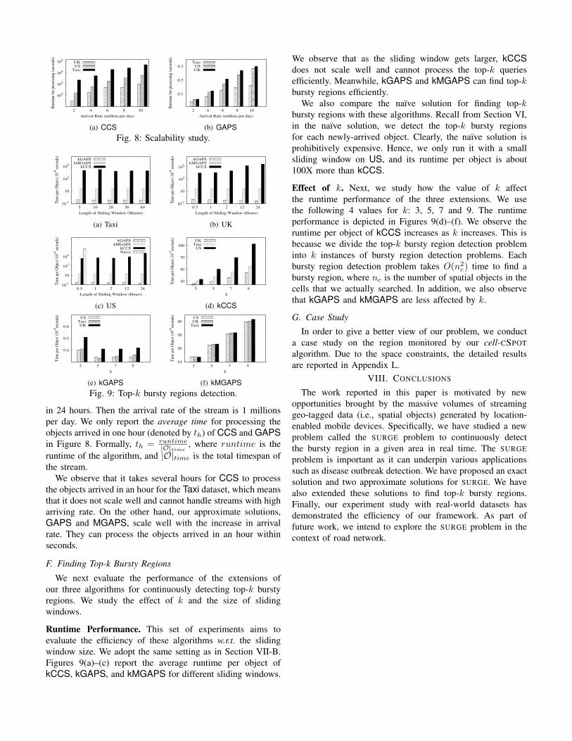
(f) kMGAPSFig. 9: Top-k bursty regions detection.

in 24 hours. Then the arrival rate of the stream is 1 millionsper day. We only report the average time for processing theobjects arrived in one hour (denoted by th) of CCS and GAPSin Figure 8. Formally, th = runtime

|O|time, where runtime is the

runtime of the algorithm, and |O|time is the total timespan ofthe stream.

We observe that it takes several hours for CCS to processthe objects arrived in an hour for the Taxi dataset, which meansthat it does not scale well and cannot handle streams with higharriving rate. On the other hand, our approximate solutions,GAPS and MGAPS, scale well with the increase in arrivalrate. They can process the objects arrived in an hour withinseconds.

F. Finding Top-k Bursty Regions

We next evaluate the performance of the extensions ofour three algorithms for continuously detecting top-k burstyregions. We study the effect of k and the size of slidingwindows.

Runtime Performance. This set of experiments aims toevaluate the efficiency of these algorithms w.r.t. the slidingwindow size. We adopt the same setting as in Section VII-B.Figures 9(a)–(c) report the average runtime per object ofkCCS, kGAPS, and kMGAPS for different sliding windows.

We observe that as the sliding window gets larger, kCCSdoes not scale well and cannot process the top-k queriesefficiently. Meanwhile, kGAPS and kMGAPS can find top-kbursty regions efficiently.

We also compare the naı̈ve solution for finding top-kbursty regions with these algorithms. Recall from Section VI,in the naı̈ve solution, we detect the top-k bursty regionsfor each newly-arrived object. Clearly, the naı̈ve solution isprohibitively expensive. Hence, we only run it with a smallsliding window on US, and its runtime per object is about100X more than kCCS.

Effect of k. Next, we study how the value of k affectthe runtime performance of the three extensions. We usethe following 4 values for k: 3, 5, 7 and 9. The runtimeperformance is depicted in Figures 9(d)–(f). We observe theruntime per object of kCCS increases as k increases. This isbecause we divide the top-k bursty region detection probleminto k instances of bursty region detection problems. Eachbursty region detection problem takes O(n2c) time to find abursty region, where nc is the number of spatial objects in thecells that we actually searched. In addition, we also observethat kGAPS and kMGAPS are less affected by k.

G. Case Study

In order to give a better view of our problem, we conducta case study on the region monitored by our cell-CSPOTalgorithm. Due to the space constraints, the detailed resultsare reported in Appendix L.

VIII. CONCLUSIONS

The work reported in this paper is motivated by newopportunities brought by the massive volumes of streaminggeo-tagged data (i.e., spatial objects) generated by location-enabled mobile devices. Specifically, we have studied a newproblem called the SURGE problem to continuously detectthe bursty region in a given area in real time. The SURGEproblem is important as it can underpin various applicationssuch as disease outbreak detection. We have proposed an exactsolution and two approximate solutions for SURGE. We havealso extended these solutions to find top-k bursty regions.Finally, our experiment study with real-world datasets hasdemonstrated the efficiency of our framework. As part offuture work, we intend to explore the SURGE problem in thecontext of road network.

REFERENCES

[1] C. C. Aggarwal, J. Han, J. Wang, and P. S. Yu. A frameworkfor clustering evolving data streams. In Proceedings of the VLDBEndowment, pages 81–92. VLDB Endowment, 2003.

[2] D. Amagata and T. Hara. Monitoring maxrs in spatial data streams. InEDBT, pages 317–328, 2016.

[3] A. Bulut and A. K. Singh. A unified framework for monitoring datastreams in real time. In International Conference on Data Engineering,pages 44–55. IEEE, 2005.

[4] X. Cao, G. Cong, C. S. Jensen, and M. L. Yiu. Retrieving regionsof interest for user exploration. Proceedings of the VLDB Endowment,7(9):733–744, 2014.

[5] L. Chen, G. Cong, and X. Cao. An efficient query indexing mechanismfor filtering geo-textual data. In Proceedings of the SIGMOD, pages749–760. ACM, 2013.

[6] L. Chen, G. Cong, X. Cao, and K.-L. Tan. Temporal spatial-keyword top-k publish/subscribe. In International Conference on Data Engineering,pages 255–266. IEEE, 2015.

[7] D.-W. Choi, C.-W. Chung, and Y. Tao. A scalable algorithm formaximizing range sum in spatial databases. Proceedings of the VLDBEndowment, 5(11):1088–1099, 2012.

[8] G. Cormode and S. Muthukrishnan. An improved data stream summary:the count-min sketch and its applications. Journal of Algorithms,55(1):58–75, 2005.

[9] A. Das, J. Gehrke, and M. Riedewald. Approximate join processingover data streams. In Proceedings of the SIGMOD. ACM, 2003.

[10] K. Feng, G. Cong, S. S. Bhowmick, W.-C. Peng, and C. Miao.Towards best region search for data exploration. In Proceedings of theInternational Conference on Management of Data, pages 1055–1070.ACM, 2016.

[11] G. P. C. Fung, J. X. Yu, P. S. Yu, and H. Lu. Parameter free bursty eventsdetection in text streams. In Proceedings of the VLDB Endowment, pages181–192. VLDB Endowment, 2005.

[12] H. Hu, Y. Liu, G. Li, J. Feng, and K.-L. Tan. A location-aware pub-lish/subscribe framework for parameterized spatio-textual subscriptions.In International Conference on Data Engineering, pages 711–722. IEEE,2015.

[13] M. M.-u. Hussain, G. Trajcevski, K. A. Islam, and M. E. Ali. Towardsefficient maintenance of continuous maxrs query for trajectories. InEDBT, 2017.

[14] C. S. Jensen, D. Lin, B. C. Ooi, and R. Zhang. Effective density querieson continuouslymoving objects. In International Conference on DataEngineering, pages 71–71. IEEE, 2006.

[15] J. Kleinberg. Bursty and hierarchical structure in streams. Data Miningand Knowledge Discovery, 7(4):373–397, 2003.

[16] Y. Kou, C.-T. Lu, and D. Chen. Spatial weighted outlier detection. InProceedings of the 2006 SIAM international conference on data mining,pages 614–618. SIAM, 2006.

[17] T. Lappas, M. R. Vieira, D. Gunopulos, and V. J. Tsotras. Onthe spatiotemporal burstiness of terms. Proceedings of the VLDBEndowment, 5(9):836–847, 2012.

[18] G. Li, Y. Wang, T. Wang, and J. Feng. Location-aware publish/subscribe.In Proceedings of the SIGKDD. ACM, 2013.

[19] J. Liu, G. Yu, and H. Sun. Subject-oriented top-k hot region queries inspatial dataset. In Proceedings of the Conference on Information andKnowledge Management, pages 2409–2412, 2011.

[20] C.-T. Lu, D. Chen, and Y. Kou. Algorithms for spatial outlier detection.In International Conference on Data Mining, pages 597–600. IEEE,2003.

[21] M. Mathioudakis, N. Bansal, and N. Koudas. Identifying, attributingand describing spatial bursts. Proceedings of the VLDB Endowment,3(1-2):1091–1102, 2010.

[22] S. C. Nandy and B. B. Bhattacharya. A unified algorithm for find-ing maximum and minimum object enclosing rectangles and cuboids.Computers & Mathematics with Applications, 29(8):45–61, 1995.

[23] J. Ni and C. V. Ravishankar. Pointwise-dense region queries in spatio-temporal databases. In International Conference on Data Engineering,pages 1066–1075. IEEE, 2007.

[24] L. O’callaghan, N. Mishra, A. Meyerson, S. Guha, and R. Motwani.Streaming-data algorithms for high-quality clustering. In InternationalConference on Data Engineering, 2002.

[25] Y. Tao, X. Hu, D.-W. Choi, and C.-W. Chung. Approximate maxrs inspatial databases. Proceedings of the VLDB Endowment, 6(13):1546–1557, 2013.

[26] X. Wang, C. Zhai, X. Hu, and R. Sproat. Mining correlated bursty topicpatterns from coordinated text streams. In Proceedings of the 13th ACMSIGKDD, pages 784–793. ACM, 2007.

[27] X. Wang, Y. Zhang, W. Zhang, X. Lin, and Z. Huang. Skype: top-kspatial-keyword publish/subscribe over sliding window. Proceedings ofthe VLDB Endowment, 9(7):588–599, 2016.

[28] X. Wang, Y. Zhang, W. Zhang, X. Lin, and W. Wang. Selectivityestimation on streaming spatio-textual data using local correlations.Proceedings of the VLDB Endowment, 8(2):101–112, 2014.

[29] X. Wang, Y. Zhang, W. Zhang, X. Lin, and W. Wang. Ap-tree: Efficientlysupport continuous spatial-keyword queries over stream. In 2015 IEEE31st International Conference on Data Engineering, pages 1107–1118.IEEE, 2015.

[30] C. Zhang, G. Zhou, Q. Yuan, H. Zhuang, Y. Zheng, L. M. Kaplan,S. Wang, and J. Han. Geoburst: Real-time local event detection in geo-tagged tweet streams. In Proceedings of the International conferenceon Research and Development in Information Retrieval, pages 513–522,2016.

[31] J. Zhao, C.-T. Lu, and Y. Kou. Detecting region outliers in meteorolog-ical data. In Proceedings of the 11th ACM international symposium onAdvances in geographic information systems, pages 49–55. ACM, 2003.

[32] Y. Zhu and D. Shasha. Efficient elastic burst detection in data streams.In Proceedings of the ninth ACM SIGKDD. ACM, 2003.

APPENDIX

A. Proof for Theorem 1

Proof: Let p be any point in the CSPOT problem, and rbe the rectangular region of size a× b whose top-right corneris located at p. A spatial object o is in r iff the correspondingrectangle object g can cover p. Since the corresponding o andg have the same creation time and weight, we can derive thatf(r,Wc) = f(p,Wc), f(r,Wp) = f(p,Wp), and thus r andp have the same burst score. As a result, if the point pm hasthe maximum burst score in the CSPOT problem, then rm alsohas the maximum burst score in the SURGE problem.

B. Proof for Lemma 2

Proof: We have

S(p) = αmax(f(p,Wc)− f(p,Wp), 0) + (1− α)f(p,Wc)

≤ αf(p,Wc) + (1− α)f(p,Wc) = f(p,Wc) = Us(c)

C. Proof for Lemma 3

Proof: Let ∆S(p), ∆f(p,W ) be the increase of S(p)and f(p,W ) after e happens, respectively. We discuss thefollowing three cases.Case 1: e is new. For any point p that is covered by g, itscurrent score is increased by ∆f(p,Wc) = g.w

|Wc| . We have∆S(p) ≤ ∆f(p,Wc) = g.w

|Wc| .Case 2: e is grown. For any point p that is covered by g, itscurrent score is decreased, i.e., ∆f(p,Wc) = − g.w

|Wc| , and itspast score is increased, i.e., ∆f(p,Wp) = g.w

|Wp| . Thus, we caneasily get ∆S(p) ≤ 0.Case 3: e is expired. For any point p covered by g,its current score is not affected, and its past score is de-creased, i.e., ∆f(p,Wp) = − g.w

|Wp| . Thus, we have ∆S(p) ≤α(−∆f(p,Wp)) = α g.w

|Wp| .Since ∆S(p) ≤ ∆Ud(c), we still have S(p) ≤ Ud(c).

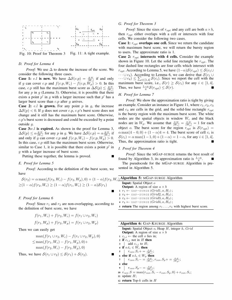
Fig. 10: Proof for Theorem 3 Fig. 11: A tight example.

D. Proof for Lemma 4

Proof: We use ∆ to denote the increase of the score. Weconsider the following three cases.Case 1: e.l is new. We have ∆S(c.p) = g.w

|Wc| if and onlyif g can cover c.p and f(c.p,Wc) − f(c.p,Wp) > 0. In thiscase, c.p still has the maximum burst score as ∆S(p) ≤ g.w

|Wc|for any p in g (Lemma 3). Otherwise, it is possible that thereexists a point p′ in g with a larger increase such that p′ has alarger burst score than c.p after g arrives.Case 2: e.l is grown. For any point p in g, the increase∆S(p) < 0. If g does not cover c.p, c.p’s burst score does notchange and it still has the maximum burst score. Otherwise,c.p’s burst score is decreased and could be exceeded by a pointoutside g.Case 3:e.l is expired. As shown in the proof for Lemma 3,∆S(p) ≤ α g.w

|Wc| for any p in g. We have ∆S(c.p) = α g.w|Wc| if

and only if g can cover c.p and f(c.p,Wc)− f(c.p,Wp) > 0.In this case, c.p still has the maximum burst score. Otherwise,similar to Case 1, it is possible that there exists a point p′ ing with a larger increase of burst score.

Putting these together, the lemma is proved.

E. Proof for Lemma 5

Proof: According to the definition of the burst score, wehave

S(r2) = αmax(f(r2,Wc)− f(r2,Wp), 0) + (1− α)f(r2,Wc)

≥(1− α)f(r2,Wc) ≥ (1− α)f(r1,Wc) ≥ (1− α)S(r1)

F. Proof for Lemma 6

Proof: Since r1 and r2 are non-overlapping, according tothe definition of burst score, we have

f(r1,Wc) + f(r2,Wc) = f(r1 ∪ r2,Wc)

f(r1,Wp) + f(r2,Wp) = f(r1 ∪ r2,Wp)

Then we can easily get

max(f(r1 ∪ r2,Wc)− f(r1 ∪ r2,Wp), 0)

≤max(f(r1,Wc)− f(r1,Wp), 0)+

max(f(r2,Wc)− f(r2,Wp), 0)

Thus, we have S(r1 ∪ r2) ≤ S(r1) + S(r2).

G. Proof for Theorem 3

Proof: Since the sizes of ropt and any cell are both a×b,then ropt either overlaps with a cell or intersects with fourcells. We consider the following two cases.Case 1: ropt overlaps one cell. Since we return the candidatewith maximum burst score, we will return the bursty regionto users. The approximate ratio is 1.Case 2: ropt intersects with 4 cells. Consider the exampleshown in Figure 10. Let the solid line rectangle be ropt. Thefour dashed line rectangles are four cells which intersect withropt. According to Lemma 5, we have (1−α)S(ropt) ≤ S(c1∪· · · ∪ c4). According to Lemma 6, we can derive that S(c1 ∪· · · ∪ c4) ≤

∑i∈[1,4] S(ci). Since we report the cell with the

maximum burst score, i.e., S(r) ≥ S(ci) for any i ∈ [1, 4].Thus, we have 1−α

4 S(ropt) ≤ S(r).

H. Proof for Lemma 7

Proof: We show the approximation ratio is tight by givingan example. Consider an instance in Figure 11, where c1, c2, c3and c4 are cells in the grid, and the solid-line rectangle roptis the bursty region with the maximum burst score. The whitenodes are the spatial objects in window Wc and the blacknodes are in Wp. We assume that o.w

|Wc| = o.w|Wp| = 1 for each

object o. The burst score for the region ropt is S(ropt) =αmax(4− 0, 0) + (1− α)4 = 4. The burst score of cell ci isS(ci) = αmax(1−1, 0) + (1−α) = 1−α, for any i ∈ [1, 4].Thus, the approximation ratio is tight.

I. Proof for Theorem 4

Proof: Since the MGAP-SURGE returns the best result offound by Algorithm 3, its approximation ratio is 1−α

4 .The pseudocode for the MGAP-SURGE Algorithm is pre-

sented in Algorithm 5.

Algorithm 5: MGAP-SURGE AlgorithmInput: Spatial Object oOutput: A region of size a× b

1 r1 ← GAP-SURGE(Grid1, o,H1);2 r2 ← GAP-SURGE(Grid2, o,H2);3 r3 ← GAP-SURGE(Grid3, o,H3);4 r4 ← GAP-SURGE(Grid4, o,H4);5 return The region among r1 . . . , r4 with highest burst score.

Algorithm 6: GAP-KSURGE AlgorithmInput: Spatial Object o, Heap H , integer k, GridOutput: A region of size a× b

1 ci,j ← the cell o lies in;2 if ci,j not in H then3 add ci,j to H;4 if o.tc ∈Wc then5 rcan.Sc+ = o.ρ

|Wc| ;6 else if o.tc ∈Wp then7 rcan.Sc− = o.ρ

|Wc| , rcan.Sp+ = o.ρ|Wp| ;

8 else9 rcan.Sp− = o.ρ

|Wp| ;10 rcan.S = max(rcan.Sc − rcan.Sp, 0) + rcan.Sc;11 update H;12 return Top-k cells in H

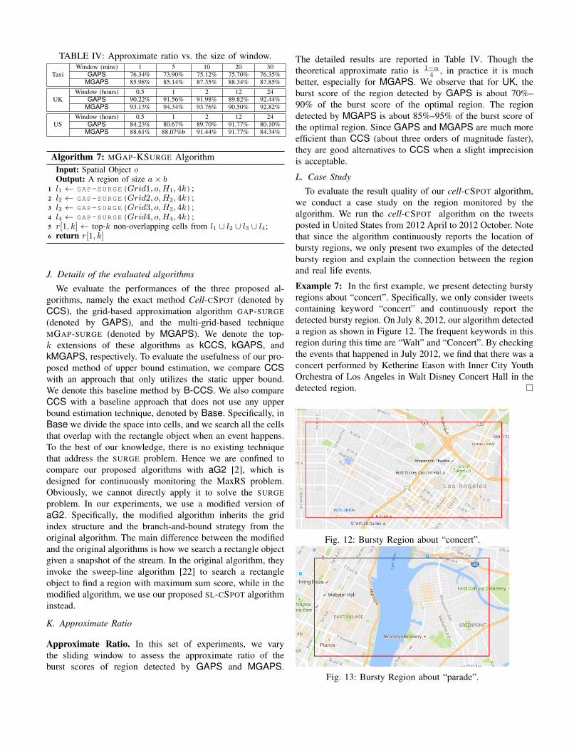
TABLE IV: Approximate ratio vs. the size of window.

TaxiWindow (mins) 1 5 10 20 30

GAPS 76.34% 73.90% 75.12% 75.70% 76.35%MGAPS 85.98% 85.14% 87.35% 88.34% 87.85%

UKWindow (hours) 0.5 1 2 12 24

GAPS 90.22% 91.56% 91.98% 89.82% 92.44%MGAPS 93.13% 94.34% 93.76% 90.50% 92.82%

USWindow (hours) 0.5 1 2 12 24

GAPS 84.23% 80.67% 89.70% 91.77% 80.10%MGAPS 88.61% 88.07%b 91.44% 91.77% 84.34%

Algorithm 7: MGAP-KSURGE AlgorithmInput: Spatial Object oOutput: A region of size a× b

1 l1 ← GAP-SURGE(Grid1, o,H1, 4k);2 l2 ← GAP-SURGE(Grid2, o,H2, 4k);3 l3 ← GAP-SURGE(Grid3, o,H3, 4k);4 l4 ← GAP-SURGE(Grid4, o,H4, 4k);5 r[1, k]← top-k non-overlapping cells from l1 ∪ l2 ∪ l3 ∪ l4;6 return r[1, k]

J. Details of the evaluated algorithms

We evaluate the performances of the three proposed al-gorithms, namely the exact method Cell-CSPOT (denoted byCCS), the grid-based approximation algorithm GAP-SURGE(denoted by GAPS), and the multi-grid-based techniqueMGAP-SURGE (denoted by MGAPS). We denote the top-k extensions of these algorithms as kCCS, kGAPS, andkMGAPS, respectively. To evaluate the usefulness of our pro-posed method of upper bound estimation, we compare CCSwith an approach that only utilizes the static upper bound.We denote this baseline method by B-CCS. We also compareCCS with a baseline approach that does not use any upperbound estimation technique, denoted by Base. Specifically, inBase we divide the space into cells, and we search all the cellsthat overlap with the rectangle object when an event happens.To the best of our knowledge, there is no existing techniquethat address the SURGE problem. Hence we are confined tocompare our proposed algorithms with aG2 [2], which isdesigned for continuously monitoring the MaxRS problem.Obviously, we cannot directly apply it to solve the SURGEproblem. In our experiments, we use a modified version ofaG2. Specifically, the modified algorithm inherits the gridindex structure and the branch-and-bound strategy from theoriginal algorithm. The main difference between the modifiedand the original algorithms is how we search a rectangle objectgiven a snapshot of the stream. In the original algorithm, theyinvoke the sweep-line algorithm [22] to search a rectangleobject to find a region with maximum sum score, while in themodified algorithm, we use our proposed SL-CSPOT algorithminstead.

K. Approximate Ratio

Approximate Ratio. In this set of experiments, we varythe sliding window to assess the approximate ratio of theburst scores of region detected by GAPS and MGAPS.

The detailed results are reported in Table IV. Though thetheoretical approximate ratio is 1−α

4 , in practice it is muchbetter, especially for MGAPS. We observe that for UK, theburst score of the region detected by GAPS is about 70%–90% of the burst score of the optimal region. The regiondetected by MGAPS is about 85%–95% of the burst score ofthe optimal region. Since GAPS and MGAPS are much moreefficient than CCS (about three orders of magnitude faster),they are good alternatives to CCS when a slight imprecisionis acceptable.

L. Case Study

To evaluate the result quality of our cell-CSPOT algorithm,we conduct a case study on the region monitored by thealgorithm. We run the cell-CSPOT algorithm on the tweetsposted in United States from 2012 April to 2012 October. Notethat since the algorithm continuously reports the location ofbursty regions, we only present two examples of the detectedbursty region and explain the connection between the regionand real life events.

Example 7: In the first example, we present detecting burstyregions about “concert”. Specifically, we only consider tweetscontaining keyword “concert” and continuously report thedetected bursty region. On July 8, 2012, our algorithm detecteda region as shown in Figure 12. The frequent keywords in thisregion during this time are “Walt” and “Concert”. By checkingthe events that happened in July 2012, we find that there was aconcert performed by Ketherine Eason with Inner City YouthOrchestra of Los Angeles in Walt Disney Concert Hall in thedetected region. �

Fig. 12: Bursty Region about “concert”.

Fig. 13: Bursty Region about “parade”.

Example 8: In the second example, we present detectingbursty regions about “parade”. On May 19, 2012, our algo-rithm detected a region as shown in Figure 13. The frequentkeywords in this region are “annual”, “dance”, and “parade”.

By checking the events that happened in May 2012, we noticedthat the dance parade is an annual parade and festival in NewYork. Specifically, in 2012 the parade took over BroadwayStreet on May 19th. �