Electronic copy available at: http://ssrn.com/abstract=2627354

Surprised by the Gambler’s and Hot Hand Fallacies? A Truth inthe Law of Small Numbers

Joshua B. Miller and Adam Sanjurjo ∗†‡

September 24, 2015

Abstract

We find a subtle but substantial bias in a standard measure of the conditional dependenceof present outcomes on streaks of past outcomes in sequential data. The mechanism is a form ofselection bias, which leads the empirical probability (i.e. relative frequency) to underestimatethe true probability of a given outcome, when conditioning on prior outcomes of the same kind.The biased measure has been used prominently in the literature that investigates incorrect beliefsin sequential decision making—most notably the Gambler’s Fallacy and the Hot Hand Fallacy.Upon correcting for the bias, the conclusions of some prominent studies in the literature arereversed. The bias also provides a structural explanation of why the belief in the law of smallnumbers persists, as repeated experience with finite sequences can only reinforce these beliefs,on average.

JEL Classification Numbers: C12; C14; C18;C19; C91; D03; G02.Keywords: Law of Small Numbers; Alternation Bias; Negative Recency Bias; Gambler’s Fal-

lacy; Hot Hand Fallacy; Hot Hand Effect; Sequential Decision Making; Sequential Data; SelectionBias; Finite Sample Bias; Small Sample Bias.

∗Miller: Department of Decision Sciences and IGIER, Bocconi University, Sanjurjo: Fundamentos del Analisis Economico,Universidad de Alicante. Financial support from the Department of Decision Sciences at Bocconi University, and the SpanishMinistry of Economics and Competitiveness under project ECO2012-34928 is gratefully acknowledged.†Both authors contributed equally, with names listed in alphabetical order.‡This draft has benefitted from helpful comments and suggestions, for which we would like to thank David

Arathorn, Maya Bar-Hillel, Gary Charness, Vincent Crawford, Martin Dufwenberg, Andrew Gelman, Daniel Gold-stein, Daniel Houser, Daniel Kahan, Daniel Kahneman, Mark Machina, Justin Rao, Yosef Rinott, Aldo Rustichiniand Daniel Stone. We would also like to thank the many seminar participants at Microsoft Research, George MasonUniversity, the Choice Lab at NHH Norway, USC, UCSD’s Rady School of Management, Chapman University, aswell as conference participants at the 11th World Congress of The Econometric Society, The 30th Annual Congress ofthe European Economic Association, and the 14th TIBER Symposium on Psychology and Economics. All mistakesand omissions remain our own.

1

Electronic copy available at: http://ssrn.com/abstract=2627354

We shall encounter theoretical conclusions which not only are unexpected but actually

come as a shock to intuition and common sense. They will reveal that commonly accepted

notions concerning chance fluctuations are without foundation and that the implications

of the law of large numbers are widely misconstrued. (Feller 1968)

1 Introduction

Jack takes a coin from his pocket and decides that he will flip it 4 times in a row, writing down

the outcome of each flip on a scrap of paper. After he is done flipping, he will look at the flips that

immediately followed an outcome of heads, and compute the relative frequency of heads on those

flips. Because the coin is fair, Jack of course expects this empirical probability of heads to be equal

to the true probability of flipping a heads: 0.5. Shockingly, Jack is wrong. If he were to sample one

million fair coins and flip each coin 4 times, observing the conditional relative frequency for each

coin, on average the relative frequency would be approximately 0.4.

We demonstrate that in a finite sequence generated by i.i.d. Bernoulli trials with probability of

success p, the relative frequency of success on those trials that immediately follow a streak of one,

or more, consecutive successes is expected to be strictly less than p, i.e. the empirical probability

of success on such trials is a biased estimator of the true conditional probability of success. While,

in general, the bias does decrease as the sequence gets longer, for a range of sequence (and streak)

lengths often used in empirical work it remains substantial, and increases in streak length.

This result has considerable implications for the study of decision making in any environment

that involves sequential data. For one, it provides a structural explanation for the persistence

of one of the most well-documented, and robust, systematic errors in beliefs regarding sequential

data—that people have an alternation bias (also known as negative recency bias; see Bar-Hillel and

Wagenaar [1991]; Nickerson [2002]; Oskarsson, Boven, McClelland, and Hastie [2009]) —by which

they believe, for example, that when observing multiple flips of a fair coin, an outcome of heads is

more likely to be followed by a tails than by another heads, as well as the closely related gambler’s

fallacy (see Bar-Hillel and Wagenaar (1991); Rabin (2002)), in which this alternation bias increases

with the length of the streak of heads. Accordingly, the result is consistent with the types of

subjective inference that have been conjectured in behavioral models of the law of small numbers,

2

as in Rabin (2002); Rabin and Vayanos (2010). Further, the result shows that data in the hot hand

fallacy literature (see Gilovich, Vallone, and Tversky [1985] and Miller and Sanjurjo [2014, 2015])

has been systematically misinterpreted by researchers; for those trials that immediately follow a

streak of successes, observing that the relative frequency of success is equal to the overall base rate

of success, is in fact evidence in favor of the hot hand, rather than evidence against it. Tying these

two implications together, it becomes clear why the inability of the gambler to detect the fallacy of

his belief in alternation has an exact parallel with the researcher’s inability to detect his mistake

when concluding that experts’ belief in the hot hand is a fallacy.

In addition, the result may have implications for evaluation and compensation systems. That

a coin is expected to exhibit an alternation “bias” in finite sequences implies that the outcome of a

flip can be successfully “predicted” in finite sequences at a rate better than that of chance (if one

is free to choose when to predict). As a stylized example, suppose that each day a stock index goes

either up or down, according to a random walk in which the probability of going up is, say, 0.6.

A financial analyst who can predict the next day’s performance on the days she chooses to, and

whose predictions are evaluated in terms of how her success rate on predictions in a given month

compares to that of chance, can expect to outperform this benchmark by using any of a number of

different decision rules. For instance, she can simply predict “up” immediately following down days,

or increase her expected relative performance even further by predicting “up” only immediately

following longer streaks of consecutive down days.1

Intuitively, it seems impossible that in a sequence of fair coin flips, we are expected to observe

tails more often than heads on those flips that have been randomly “assigned” to immediately

follow a heads. While this intuition is appealing, it ignores the sequential structure of the data,

and thus overlooks that there is a selection bias towards observing tails when forming the group of

flips that immediately follow a heads.2 In order to see the intuition behind this selection bias, it is

1Similarly, it is easy to construct betting games that act as money pumps. For example, we can offer the followinglottery at a $5 ticket price: a fair coin will be flipped 4 times. if the relative frequency of heads on those flips thatimmediately follow a heads is greater than 0.5 then the ticket pays $10; if the relative frequency is less than 0.5 thenthe ticket pays $0; if the relative frequency is exactly equal to 0.5, or if no flip is immediately preceded by a heads,then a new sequence of 4 flips is generated. While, intuitively, it seems like the expected payout of this ticket is $0,it is actually $-0.71 (see Table 1). Curiously, this betting game would appear relatively more attractive to someonewho believes in the independence of coin flips, as compared to someone with Gambler’s Fallacy beliefs.

2The intuition also ignores that while the variable that assigns a flip to immediately follow a heads is random, itsoutcome is also included in the calculation of the relative frequency. This implies that the relative frequency is notindependent of which flips are assigned to follow a heads, e.g. for 10 flips of a fair coin if we let GH = {2, 4, 5, 8, 10}be the group of flips that immediately follow a heads, then we know that the first 9 flips of the sequence must be

3

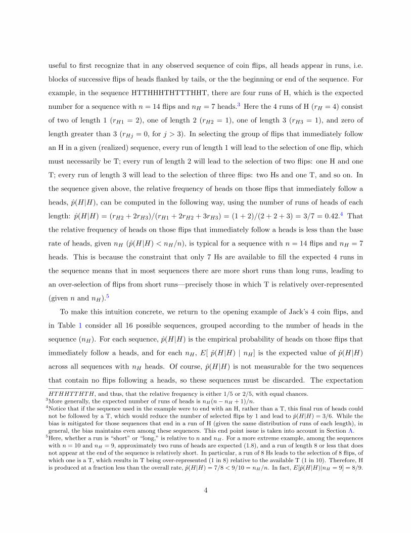
useful to first recognize that in any observed sequence of coin flips, all heads appear in runs, i.e.

blocks of successive flips of heads flanked by tails, or the the beginning or end of the sequence. For

example, in the sequence HTTHHHTHTTTHHT, there are four runs of H, which is the expected

number for a sequence with n = 14 flips and nH = 7 heads.3 Here the 4 runs of H (rH = 4) consist

of two of length 1 (rH1 = 2), one of length 2 (rH2 = 1), one of length 3 (rH3 = 1), and zero of

length greater than 3 (rHj = 0, for j > 3). In selecting the group of flips that immediately follow

an H in a given (realized) sequence, every run of length 1 will lead to the selection of one flip, which

must necessarily be T; every run of length 2 will lead to the selection of two flips: one H and one

T; every run of length 3 will lead to the selection of three flips: two Hs and one T, and so on. In

the sequence given above, the relative frequency of heads on those flips that immediately follow a

heads, p(H|H), can be computed in the following way, using the number of runs of heads of each

length: p(H|H) = (rH2 + 2rH3)/(rH1 + 2rH2 + 3rH3) = (1 + 2)/(2 + 2 + 3) = 3/7 = 0.42.4 That

the relative frequency of heads on those flips that immediately follow a heads is less than the base

rate of heads, given nH (p(H|H) < nH/n), is typical for a sequence with n = 14 flips and nH = 7

heads. This is because the constraint that only 7 Hs are available to fill the expected 4 runs in

the sequence means that in most sequences there are more short runs than long runs, leading to

an over-selection of flips from short runs—precisely those in which T is relatively over-represented

(given n and nH).5

To make this intuition concrete, we return to the opening example of Jack’s 4 coin flips, and

in Table 1 consider all 16 possible sequences, grouped according to the number of heads in the

sequence (nH). For each sequence, p(H|H) is the empirical probability of heads on those flips that

immediately follow a heads, and for each nH , E[ p(H|H) | nH ] is the expected value of p(H|H)

across all sequences with nH heads. Of course, p(H|H) is not measurable for the two sequences

that contain no flips following a heads, so these sequences must be discarded. The expectation

HTHHTTHTH, and thus, that the relative frequency is either 1/5 or 2/5, with equal chances.3More generally, the expected number of runs of heads is nH(n− nH + 1)/n.4Notice that if the sequence used in the example were to end with an H, rather than a T, this final run of heads couldnot be followed by a T, which would reduce the number of selected flips by 1 and lead to p(H|H) = 3/6. While thebias is mitigated for those sequences that end in a run of H (given the same distribution of runs of each length), ingeneral, the bias maintains even among these sequences. This end point issue is taken into account in Section A.

5Here, whether a run is “short” or “long,” is relative to n and nH . For a more extreme example, among the sequenceswith n = 10 and nH = 9, approximately two runs of heads are expected (1.8), and a run of length 8 or less that doesnot appear at the end of the sequence is relatively short. In particular, a run of 8 Hs leads to the selection of 8 flips, ofwhich one is a T, which results in T being over-represented (1 in 8) relative to the available T (1 in 10). Therefore, His produced at a fraction less than the overall rate, p(H|H) = 7/8 < 9/10 = nH/n. In fact, E[p(H|H)|nH = 9] = 8/9.

4

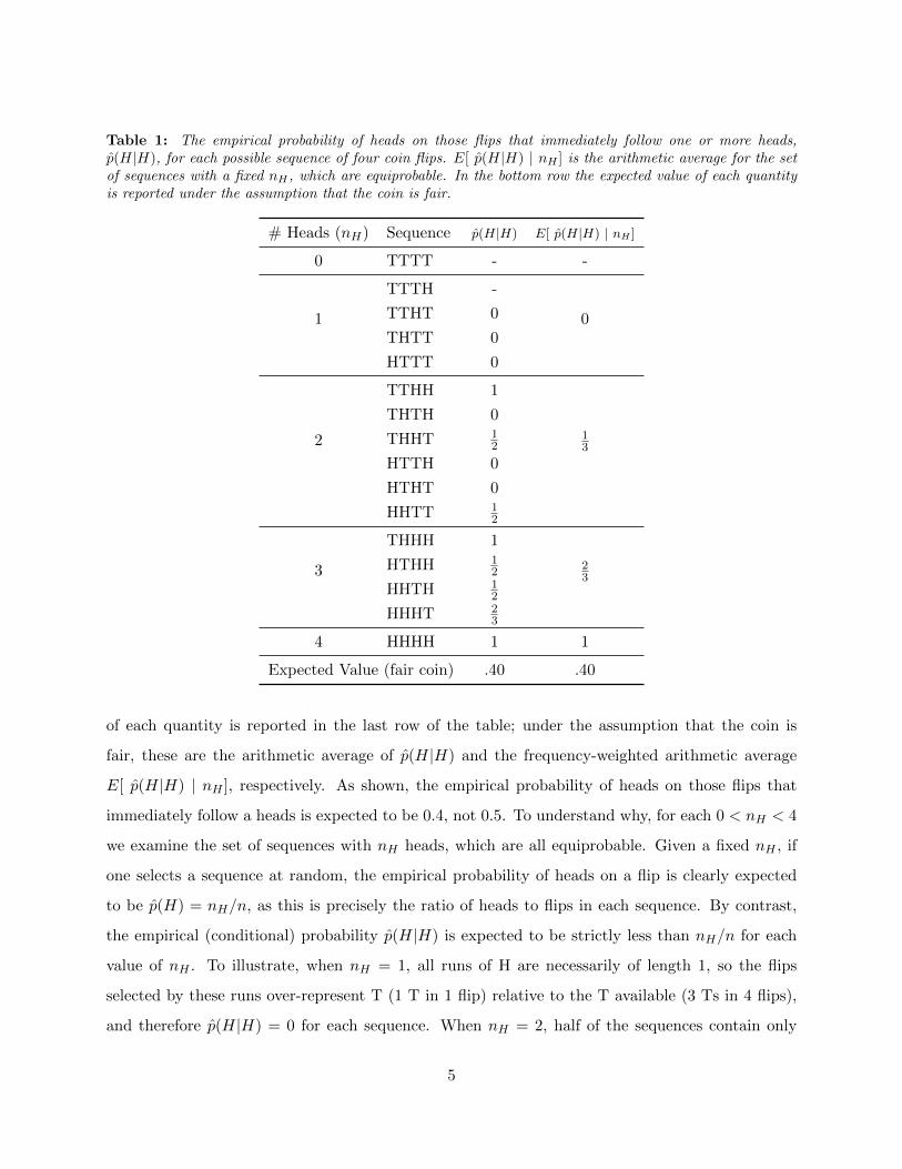
Table 1: The empirical probability of heads on those flips that immediately follow one or more heads,p(H|H), for each possible sequence of four coin flips. E[ p(H|H) | nH ] is the arithmetic average for the setof sequences with a fixed nH , which are equiprobable. In the bottom row the expected value of each quantityis reported under the assumption that the coin is fair.

# Heads (nH) Sequence p(H|H) E[ p(H|H) | nH ]

0 TTTT - -

1

TTTH -

0TTHT 0

THTT 0

HTTT 0

2

TTHH 1

13

THTH 0

THHT 12

HTTH 0

HTHT 0

HHTT 12

3

THHH 1

23

HTHH 12

HHTH 12

HHHT 23

4 HHHH 1 1

Expected Value (fair coin) .40 .40

of each quantity is reported in the last row of the table; under the assumption that the coin is

fair, these are the arithmetic average of p(H|H) and the frequency-weighted arithmetic average

E[ p(H|H) | nH ], respectively. As shown, the empirical probability of heads on those flips that

immediately follow a heads is expected to be 0.4, not 0.5. To understand why, for each 0 < nH < 4

we examine the set of sequences with nH heads, which are all equiprobable. Given a fixed nH , if

one selects a sequence at random, the empirical probability of heads on a flip is clearly expected

to be p(H) = nH/n, as this is precisely the ratio of heads to flips in each sequence. By contrast,

the empirical (conditional) probability p(H|H) is expected to be strictly less than nH/n for each

value of nH . To illustrate, when nH = 1, all runs of H are necessarily of length 1, so the flips

selected by these runs over-represent T (1 T in 1 flip) relative to the T available (3 Ts in 4 flips),

and therefore p(H|H) = 0 for each sequence. When nH = 2, half of the sequences contain only

5

runs of H of length 1, and the other half contain only runs of H of length 2. Therefore, the flips

selected by these runs either over-represent T (1 T in 1 flip), or equally represent T (1 T in 2 flips),

relative to the T available (2 Ts in 4 flips), which, on average, leads to a bias towards selecting

flips that over-represent T. When nH = 3, runs of H are of length 1,2, or 3, thus the flips taken

from any of these runs over-represent T (at least 1 T in 3 flips) relative to the T available (1

T in 4 flips).6 These facts reflect the constraint that the total number of Hs in runs of H must

equal nH (∑nH

i=1 irHi = nH) places on the joint distribution of runs of each length ((rHi)nHi=1), and

imply that for each nH , E[p(H|H)|nH ] = nH−1n−1 , which also happens to be the familiar formula for

sampling without replacement. When considering the empirical probability of a heads on those flips

that immediately follow a streak of k or more heads, p(H|kH) (see Section 2), the constraint that∑nHi=1 irHi = nH places on the joint distribution of run lengths greater than k leads to a downward

bias that is even more severe for E[p(H|kH)|nH ].7

The law of large numbers would seem to imply that as the number of coins that Jack samples

increases, the average empirical probability of heads would approach the true probability. The key

to why this is not the case, and to why the bias remains, is that it is not the flip that is treated

as the unit of analysis, but rather the sequence of flips from each coin. In particular, if Jack were

willing to assume that each sequence had been generated by the same coin, and were to compute

the empirical probability by instead pooling together all of those flips that immediately follow a

heads, regardless of which coin produced them, then the bias would converge to zero as the number

of coins approaches infinity. Therefore, in treating the sequence as the unit of analysis, the average

empirical probability across coins amounts to an unweighted average that does not account for

the number of flips that immediately follow a heads in each sequence, and thus leads the data to

appear consistent with the gambler’s fallacy.8 The implications for learning are stark: to the extent

6In order to ease exposition, this discussion ignores that sequences can also end with a run of heads. Nevertheless, whathappens at the end points of sequences is not the source of the bias. In fact, if one were to calculate p(H|H) in a circularway, so that the first position were to follow the fourth, the bias would be even more severe (E[p(H|H)] = 0.38).

7To give an idea of why E[p(H|kH)|nH ] < E[p(H|H)|nH ] for k > 1, first note that each run of length j < k leads tothe selection of 0 flips, and each run of length j ≥ k leads to the selection of j − k+ 1 flips, with j − k Hs and one T.Because nH is fixed, when k increases from 1 there are fewer possible run lengths that are greater than k, and eachyields a selection of flips that is balanced relatively more towards T. In the extreme, when k = nH , there are no runslonger than k, and only a single flip is selected in each sequence with nH heads, which yields E[p(H|kH)|nH ] = 0.

8Given this, the direction of the bias can be understood by examining Table 1; the sequences that have more flipsof heads tend to have a higher relative frequency of repetition. Thus, these higher relative frequency sequences are“underweighted” when taking the average of the relative frequencies across all (here, equiprobable) sequences, whichresults in an average that indicates alternation.

6

that decision makers update their beliefs regarding sequential dependence with the (unweighted)

empirical probabilities that they observe in finite length sequences, they can never unlearn a belief

in the gambler’s fallacy.9,10

That the bias emerges when the empirical conditional probability—the estimator of conditional

probability—is computed for finite sequences, suggests a connection to the well-known finite sample

bias of the least squares estimator of autocorrelation in time series data (Stambaugh 1986; Yule

1926). Indeed, we find that this connection is more than suggestive: by letting x ∈ {0, 1}n be

a sequence of iid Bernoulli(p) trials, and P(xi = 1|xi−1 = · · · = xi−k = 1) the probability of a

success in trial i, one can see that conditional on a success streak of length k (or more) on the

immediately preceding k trials, the least squares estimator for the coefficients in the associated

linear probability model, xi = β0 + β11[xi−1=···=xi−k=1](i), happens to be the conditional relative

frequency p(xi = 1|xi−1 = · · · = xi−k = 1). Therefore, the explicit formula for the bias that we

find below can be applied directly to the coefficients of the associated linear probability model

(see Appendix D). Furthermore, the bias in the associated statistical test can be corrected with

an appropriate form of re-sampling, analogous to what has been done in the study of time series

data (Nelson and Kim 1993), but in this case using permutation test procedures (see Miller and

Sanjurjo [2014] for details).11

In Section 2 (and Appendix B), we derive an explicit formula for the empirical probability of

success on trails that immediately follow a streak of success, for any probability of success p, any

streak length k, and any sample size n. While this formula does not appear, in general, to admit

a closed form representation, for the special case of streaks of length k = 1 (as in the example

9For a full discussion see Section 3.10When learning is deliberate, rather than intuitive, this result also holds if empirical probabilities are instead repre-

sented as natural frequencies (e.g. 3 in 4, rather than .75), under the assumption that people neglect sample size (seeKahneman and Tversky (1972), and Benjamin, Rabin, and Raymond (2014)).

11In a comment on this paper, Rinott and Bar-Hillel (2015) assert that the work of Bai (1975) (and references therein)demonstrate that the bias in the conditional relative frequency follows directly from known results on the bias ofMaximum Likelihood estimators of transition probabilities in Markov chains, as independent Bernoulli trials can berepresented by a Markov chain with each state defined by the sequence of outcomes in the previous k trials. Whileit is true that the MLE of the corresponding transition matrix is biased, the cited theorems do not apply in this casebecause they require that transition probabilities in different rows of the transition matrix not be functions of eachother, and not be equal to zero, a requirement which does not hold in the corresponding transition matrix. Instead,an unbiased estimator of each transition probability will exist, and will be a function of the unconditional relativefrequency. Rinott and Bar-Hillel (2015) also provide a novel alternative proof for the case of k = 1 that providesreasoning which suggests sampling-without-replacement as the mechanism behind the bias. This reasoning does notextend to the case of k > 1, due to the combinatorial nature of the problem. For an intuition why sampling-without-replacement reasoning does not fully explain the bias, see Appendix C.

7

above) one is provided. For k larger than one, we use analogous reasoning to compute the expected

empirical probability for sequences with lengths relevant for empirical work, using results on the

sampling distribution developed in Appendix B.

Section 3 begins by detailing how the result provides a structural explanation of the persistence

of both alternation bias, and gambler’s fallacy beliefs. In addition, results are reported from a

simple survey that we conducted in order to gauge whether the degree of alternation bias that

has typically been observed from experimental subjects in previous studies is roughly consistent

with subjects’ experience with finite sequences outside of the laboratory. Then we discuss how

the result reveals an incorrect assumption made in the analyses of the most prominent hot hand

fallacy studies, and outline how to correct for the bias in statistical testing. Once corrected for, the

previous findings are reversed.

2 Result

We find an explicit formula for the expected conditional relative frequency of a success in a finite

sequence of i.i.d. Bernoulli trials with any probability of success p, any sequence length n, and

when conditioning on streaks of successes of any length k. Further, we quantify the bias for a range

of n and k relevant for empirical work. In this section, for the simplest case of k = 1, we present a

closed form representation of this formula. To ease exposition, the statement and proofs of results

for k larger than one are treated in Appendix B.

2.1 Expected Bias

Let X1, . . . , Xn be a sequence of n i.i.d Bernoulli trials with probability of success p := P(Xi = 1).

Let the sequence x = (x1, ..., xn) ∈ {0, 1}n be the realization of the n trials, N1(x) :=∑n

i=1 xi the

number of ones, and N0(x) := n−N1(x) the number of zeros, with their respective realizations n1

and n0. We begin with two definitions.

Definition 1 For x ∈ {0, 1}n, n1 ≥ 0, and k = 1, . . . , n1, the set of k/1-streak successors I1k(x)

is the subset of trials that immediately succeed a streak of ones of length k or more, i.e.

I1k(x) := {i ∈ {k + 1, . . . , n} : xi−1 = · · · = xi−k = 1}

8

The k/1-streak momentum statistic P1k(x) is the relative frequency of 1, for the subset of trials

that are k/1-streak successors, i.e.

Definition 2 For x ∈ {0, 1}n, if the set of k/1-streak successors satisfies I1k(x) 6= ∅, then the

k/1-streak momentum statistic is defined as:

P1k(x) :=

∑i∈I1k xi

|I1k(x)|

otherwise it is not defined

Thus, the momentum statistic measures the success rate on the subset of trials that immediately

succeed a streak of success(es). Now, let P1k be the derived random variable with support {p1k ∈

[0, 1] : p1k = P1k(x) for x ∈ {0, 1}n, I1k(x) 6= ∅}, and distribution determined by the Bernoulli

trials. Then the expected value of P1k is equal to the expected value of P1k(x) across all sequences

x for which P1k(x) is defined, and can be represented as follows:

E[P1k] = E[P1k(x)

∣∣∣ I1k(x) 6= ∅]

= Cn∑

n1=k

∑{x: N1(x)=n1

I1k(x)6=∅}

pn1(1− p)n−n1P1k(x)

= Cn∑

n1=k

pn1(1− p)n−n1

[(n

n1

)− U1k(n, n1)

]· E[P1k(x)

∣∣∣ I1k(x) 6= ∅, N1(x) = n1

]= C

n∑n1=k

pn1(1− p)n−n1

[(n

n1

)− U1k(n, n1)

]· E[P1k|N1 = n1] (1)

where U1k(n, n1) := |{x ∈ {0, 1}n : N1(x) = n1 & I1k(x) = ∅}| is the number of sequences for which

P1k(x) is undefined and C is the constant that normalizes the total probability to 1.12 The distri-

bution of P1k|N1 derived from x has support {p1k ∈ [0, 1] : p1k = P1k(x) for x ∈ {0, 1}n, I1k(x) =

∅, and N1(x) = n1} for all k ≥ 1 and n1 ≥ 1. In Appendix B we determine this distribution for

all k > 1. Here we consider the case of k = 1, and compute the expected value directly. First we

establish the main lemma.

12More precisely, C := 1/(

1−∑nn1=k

U1k(n, n1)pn1(1− p)n−n1

). Note that U1k =

(nn1

)when n1 < k, and U1k = 0

when n1 > (k − 1)(n− n1) + k. Also, for n1 = k, P1k(x) = 0 for all admissible x.

9

Lemma 3 For n > 1 and n1 = 1, . . . , n

E[P11|N1 = n1] =n1 − 1

n− 1(2)

Proof: See Appendix A.

The quantity E[P11(x)

∣∣∣ I1k(x) = ∅, N1(x) = n1

]can, in principle, be computed directly

by calculating P11(x) for each sequence of length n1, and then averaging across these sequences,

but the number of sequences is typically too large to perform the complete enumeration needed.13

The key to the argument is to reduce the dimensionality of the problem by identifying the set of

sequences over which P11(x) is constant (this same argument can be extended to find the conditional

expectation of P1k(x) for k > 1 in Appendix B). As discussed in Section 1, we observe that each

run of length j that does not appear at the end of the sequence contributes j trial observations to

the computation of P11(x), of which j − 1 are 1s, therefore:

P11(x) =

∑n1j=2(j − 1)R1j(x)∑n1j=1 jR1j(x)− xn

=n1 −R1(x)

n1 − xn

where R1j(x) is the number of runs of ones of length j, and R1(x) is the total number of runs of

ones.14 For all sequences with R1(x) = r1, P11(x) is (i) constant and equal to (n1 − r1)/n1 for

all those sequences that terminate with a zero, and (ii) constant and equal to (n1 − r1)/(n1 − 1)

for all those sequences that terminate with a one. The distribution of r1 in each of these cases

can be found by way of combinatorial argument, and the expectation computed directly, yielding

Equation 2.

This result is quantitatively identical to the formula one would get for the probability of success,

conditional on n1 successes and n0 = n − n1 failures, if one were to first remove one success from

an unordered set of n trials with n1 successes, and then draw one of the remaining n− 1 trials at

random, without replacement. Sampling-without-replacement reasoning can be used to provide an

13For example, with n = 100 and n1 = 50, there are 100!/(50!50!) > 1029 distinguishable sequences, which is greaterthan the nearly 1024 microseconds since the “big bang.”

14More precisely, R1j(x) := |{i ∈ {1, . . . , n} :∏i`=i−j+1 x` = 1 and, if i < n, then xi+1 = 0 and, if i > j, then xi−j =

0}|. R1(x) := |{i ∈ {1, . . . , n} : xi = 1 and, if i < n, then xi+1 = 0}|.

10

alternate proof of Lemma 3 (see Appendix A), but this reasoning does not extend to the case of

k > 1.15

Given (2), Equation 1 can now be simplified, with E[P11] expressed in terms of only n and p

Theorem 4 For p > 0

E[P11] =

[p− 1−(1−p)n

n

]nn−1

1− (1− p)n − p(1− p)n−1(3)

Proof: See Appendix A.

In the following subsection we plot E[P11] as a function of n, for several values of p, and we also

plot E[P1k] for k > 1.

In Section 3.2 we compare the relative frequency of success for k/1-streak successor trials (rep-

etitions) to the relative frequency of success for k/0-streak successor trials (alternations), which

requires explicit consideration of the expected difference between these conditional relative fre-

quencies. We now consider the case in which k = 1 (for k > 1 see Appendix B), and find the

difference to be independent of p. Before stating the theorem, we first define P0k to be the relative

frequency of a 0 for k/0-streak successor trials, i.e.

P0k(x) :=

∑i∈I0k 1− xi|I0k(x)|

where P0k is the derived distribution. We find that for k = 1, the expected difference between the

relative frequency of success for k/1-streak successor trials, and the relative frequency of success

for k/0-streak successor trials, D1 := P11 − (1− P01), depends only on n.16

Theorem 5 Letting D1 := P11 − (1− P01), then for any 0 < p < 1 and n > 2, we have:

E[D1] = − 1

n− 1

Proof: See Appendix A

15For an intuition why the sampling without replacement reasoning that worked when k = 1 does not extend to k > 1,see Appendix C.

16This independence from p does not extend to the case of k > 1; see Section 2.2, and Appendix B.2.

11

0 20 40 60 80 1000.1

0.2

0.3

0.4

0.5

0.6

0.7

0.8

n

E[P

1k]

k = 1

k = 2

k = 3

k = 4

k = 5

p = .75

p = .5

p = .25

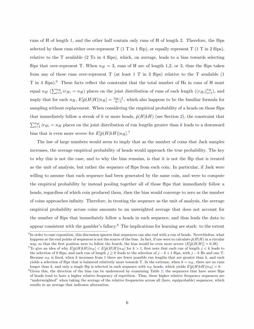
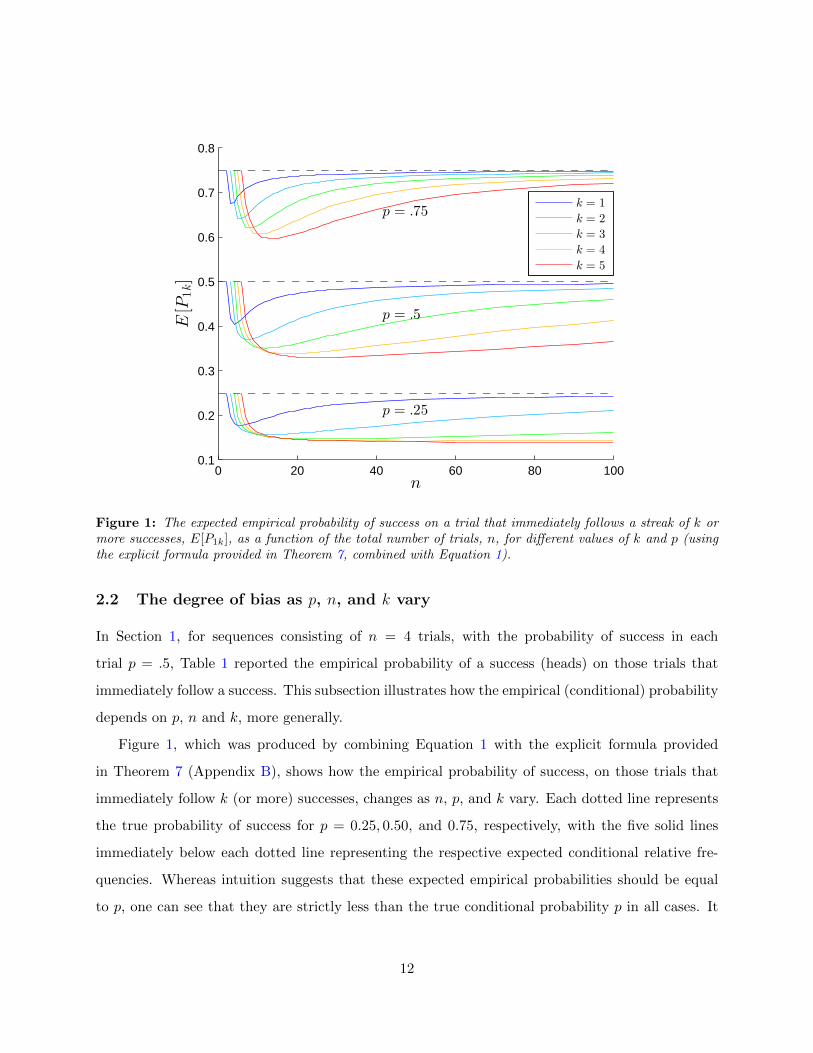
Figure 1: The expected empirical probability of success on a trial that immediately follows a streak of k ormore successes, E[P1k], as a function of the total number of trials, n, for different values of k and p (usingthe explicit formula provided in Theorem 7, combined with Equation 1).

2.2 The degree of bias as p, n, and k vary

In Section 1, for sequences consisting of n = 4 trials, with the probability of success in each

trial p = .5, Table 1 reported the empirical probability of a success (heads) on those trials that

immediately follow a success. This subsection illustrates how the empirical (conditional) probability

depends on p, n and k, more generally.

Figure 1, which was produced by combining Equation 1 with the explicit formula provided

in Theorem 7 (Appendix B), shows how the empirical probability of success, on those trials that

immediately follow k (or more) successes, changes as n, p, and k vary. Each dotted line represents

the true probability of success for p = 0.25, 0.50, and 0.75, respectively, with the five solid lines

immediately below each dotted line representing the respective expected conditional relative fre-

quencies. Whereas intuition suggests that these expected empirical probabilities should be equal

to p, one can see that they are strictly less than the true conditional probability p in all cases. It

12

0 20 40 60 80 100−0.5

−0.45

−0.4

−0.35

−0.3

−0.25

−0.2

−0.15

−0.1

−0.05

0

n

E[D

k]

0 < p < 1p = .5p = .25, .75p = .5p = .25, .75k = 1

k = 2k = 3

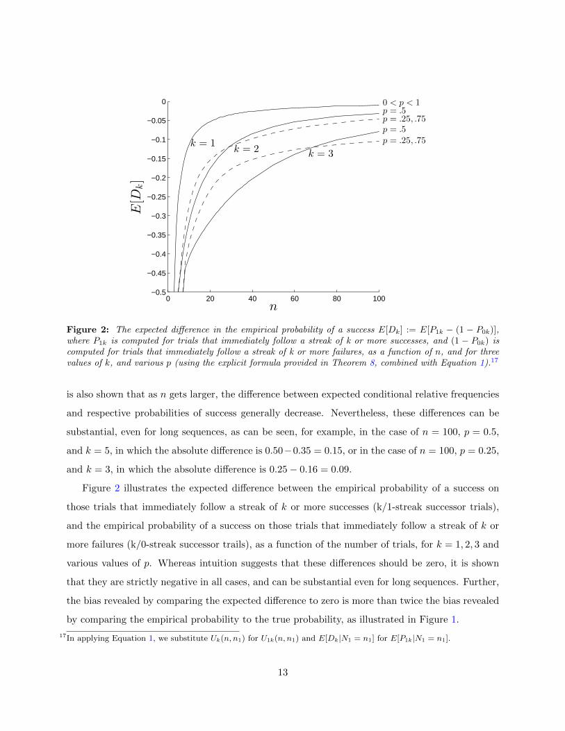
Figure 2: The expected difference in the empirical probability of a success E[Dk] := E[P1k − (1 − P0k)],where P1k is computed for trials that immediately follow a streak of k or more successes, and (1 − P0k) iscomputed for trials that immediately follow a streak of k or more failures, as a function of n, and for threevalues of k, and various p (using the explicit formula provided in Theorem 8, combined with Equation 1).17

is also shown that as n gets larger, the difference between expected conditional relative frequencies

and respective probabilities of success generally decrease. Nevertheless, these differences can be

substantial, even for long sequences, as can be seen, for example, in the case of n = 100, p = 0.5,

and k = 5, in which the absolute difference is 0.50−0.35 = 0.15, or in the case of n = 100, p = 0.25,

and k = 3, in which the absolute difference is 0.25− 0.16 = 0.09.

Figure 2 illustrates the expected difference between the empirical probability of a success on

those trials that immediately follow a streak of k or more successes (k/1-streak successor trials),

and the empirical probability of a success on those trials that immediately follow a streak of k or

more failures (k/0-streak successor trails), as a function of the number of trials, for k = 1, 2, 3 and

various values of p. Whereas intuition suggests that these differences should be zero, it is shown

that they are strictly negative in all cases, and can be substantial even for long sequences. Further,

the bias revealed by comparing the expected difference to zero is more than twice the bias revealed

by comparing the empirical probability to the true probability, as illustrated in Figure 1.

17In applying Equation 1, we substitute Uk(n, n1) for U1k(n, n1) and E[Dk|N1 = n1] for E[P1k|N1 = n1].

13

3 Applications to the Gambler’s and Hot Hand Fallacies

Inferring serial dependence of any order from sequential data is an important feature of decision

making in a variety of important economic domains, and has been studied in financial markets,18

sports wagering,19 casino gambling,20 and lotteries.21 The most controlled studies of decision

making based on sequential data have occurred in a large body of laboratory experiments (for

surveys, see Bar-Hillel and Wagenaar [1991], Nickerson [2002], Rabin [2002], and Oskarsson et al.

[2009]; for a discussion of work in the economics literature, see Miller and Sanjurjo [2014]).

First, we explain how the result from Section 2 provides a structural explanation for the persis-

tence of alternation bias and gambler’s fallacy beliefs. Then we conduct a simple survey to check

whether peoples’ experience outside of the laboratory is consistent with the degrees of alternation

bias and gambler’s fallacy that they exhibit within the laboratory. Lastly, we explain how the

result reveals a common error in the statistical analyses of the most prominent hot hand fallacy

studies (including the original), which when corrected for, reverses what is arguably the strongest

evidence that belief in the hot hand is a “cognitive illusion.” In particular, what had previously

been considered nearly conclusive evidence of a lack of hot hand performance, was instead strong

evidence of hot hand performance all along.

3.1 Alternation Bias and Gambler’s Fallacy

Why, if the gambler’s fallacy is truly fallacious, does it persist? Why is it not corrected

as a consequence of experience with random events? (Nickerson 2002)

A classic result in the literature on the human perception of randomly generated sequential

data is that people believe outcomes alternate more than they actually do, e.g. for a fair coin,

after observing a flip of a tails, people believe that the next flip is more likely to produce a heads

than a tails (Bar-Hillel and Wagenaar 1991; Nickerson 2002; Oskarsson et al. 2009; Rabin 2002).22

18Barberis and Thaler (2003); De Bondt (1993); De Long, Shleifer, Summers, and Waldmann (1991); Kahneman andRiepe (1998); Loh and Warachka (2012); Malkiel (2011); Rabin and Vayanos (2010)

19Arkes (2011); Avery and Chevalier (1999); Brown and Sauer (1993); Camerer (1989); Durham, Hertzel, and Martin(2005); Lee and Smith (2002); Paul and Weinbach (2005); Sinkey and Logan (2013)

20Croson and Sundali (2005); Narayanan and Manchanda (2012); Smith, Levere, and Kurtzman (2009); Sundali andCroson (2006); Xu and Harvey (2014)

21Galbo-Jørgensen, Suetens, and Tyran (2015); Guryan and Kearney (2008); Yuan, Sun, and Siu (2014)22This alternation bias is also sometimes referred to as negative recency bias.

14

Further, as a streak of identical outcomes increases in length, people also tend to think that the

alternation rate on the outcome that follows becomes even larger, which is known as the gambler’s

fallacy (Bar-Hillel and Wagenaar 1991).23

The result presented in Section 2 provides a structural explanation for the persistence of both

of these systematic errors in beliefs. Independent of how these beliefs arise, to the extent that

decision makers update their beliefs regarding sequential dependence with the relative frequencies

that they observe in finite length sequences, no amount of exposure to these sequences can make

a belief in the gambler’s fallacy go away. The reason why is that for any sequence length n, even

as the number of sequences observed goes to infinity, the expected rate of alternation of a given

outcome is strictly larger than the (un)conditional probability of the outcome, and this expected

rate of alternation generally grows larger when conditioning on streaks of preceding outcomes of

increasing length (see Figure 1, Section 2). Thus, experience can, in a sense, train people to have

gambler’s fallacy beliefs.24

A possible solution to the problem is that rather than observing more sequences of size n, one

could instead observe longer sequences; as n goes to infinity the difference between the conditional

relative frequency of, say, a success, and the underlying conditional probability of a success, disap-

pear. Nevertheless, this possibility may be unlikely to fix the problem, for the following reasons:

(1) these differences only go away when n is extremely large relative to the lengths of sequences

that people are likely to typically observe (as can be seen in Figure 1 and the survey results be-

low), (2) even if one were to observe sufficiently long sequences of outcomes, memory and attention

limitations may not allow them to consider more than relatively short subsequences (Bar-Hillel

and Wagenaar 1991; Cowan 2001; Miller 1956; Nickerson 2002), thus effectively converting the long

sequence into many shorter sub-sequences in which expected differences will again be relatively

23The following discussion presumes that a decision maker keeps track of the alternation rate of a particular outcome(e.g for heads, 1− p(H|H)), which is reasonable for many applications. For flips of a fair coin there may be no needto discriminate between an alternation after a flip of heads and an alternation after a flip of tails. In this case, theoverall alternation rate, (# alternations for streaks of length 1 )/(number of flips−1), is expected to be .5. It is easyto demonstrate that the alternation rate computed for any streak of length k > 1 is expected to be greater than .5(the explicit formula can be derived using an argument identical to that used in Theorem 8).

24One can imagine a decision maker who believes that θ = P(Xi = 1|Xi−1 = 1) is fixed and has a prior µ(θ) with support[0, 1]. The decision maker attends to trials that immediately follow one (or more) success I ′ := {i ∈ {2, . . . , n} :

Xi−1 = 1}, i.e. the decision maker observes the sequence Y|I′| = (Yi)|I′|i=1 = (Xι−1(i))

|I′|i=1, where ι : I ′ → {1, . . . , |I ′|},

with ι(i) = |{j ∈ I ′ : j ≤ i}|. Whenever |I ′| > 0, the posterior distribution becomes p(θ|Y|I′|) = θ∑

i Yi(1 −θ)|I

′|−∑

i Yiµ(θ)/∫θ′ θ′∑

i Yi(1− θ′)|I′|−

∑i Yiµ(θ′). If X1, . . . , Xn are iid Bernoulli(p), then with repeated exposure to

sequences of length n, µ(θ) will approach point mass on the value in Equation 3, which is less than p.

15

large.25

Another possibility is that people become able to interpret observed relative frequencies in such

a way as to make the difference between the underlying probability and expected conditional relative

frequencies small. The way of doing this, as explained briefly in Section 1, is to count the number

of observations that were used in computing the conditional relative frequency for each sequence,

and then use these as weights in a weighted average of the conditional relative frequencies across

sequences. Doing so will make the difference minimal. Nevertheless, this requires relatively more

effort, and memory capacity, and at the same time does not intuitively seem to yield any benefit

relative to the simpler and more natural approach of taking the standard (unweighted) average

relative frequency across sequences. A simpler, and equivalent, correction, is that a person could

instead pool observations from all sequences and compute the conditional relative frequency in the

new “composite” sample. While simple in theory, this seems unlikely to occur in practice due to

similar arguments, such as the immense demands on memory and attention that it would require,

combined with the apparent suitability of the more natural, and simpler, alternative approach.

Thus, one might conclude that because people are effectively only exposed to finite sequences of

outcomes, the natural learning environment is “wicked,” in the sense that it does not allow people

to calibrate to the true conditional probabilities with experience alone (Hogarth 2010).

Another example of how experience may not be helpful in ridding of alternation bias and

gambler’s fallacy beliefs is that gambling, in games such as roulette, places no pressure on these

beliefs to go away. In particular, while people can learn via reinforcement that gambling is not

profitable, they cannot learn via reinforcement that it is disadvantageous to believe in excessive

alternation, or in streak-effects, as the expected return is the same for all choices (Croson and

Sundali 2005; Rabin 2002).

Thus, while it seems unlikely that experience alone will make alternation bias and gambler’s

fallacy beliefs disappear, studies have shown that people can learn to perceive randomness correctly

25The idea that limitations in memory capacity may lead people to rely on finite samples has been investigated inKareev (2000). Interestingly, in earlier work Kareev (1992) notes that while the expected overall alternation ratefor streaks of length k = 1 is equal to 0.5 (when not distinguishing between a preceding heads or tails), people’sexperience can be made to be consistent with an alternation rate that is greater than 0.5 if the set of observablesequences that they are exposed to is restricted to those that are subjectively “typical” (e.g. those with an overallsuccess rate close to 0.5). In fact, for streaks of length k > 1, this restriction is not necessary, as the expected overallalternation rate across all sequences is greater than 0.5 (the explicit formula that demonstrates this can be derivedusing an argument identical to that used in Theorem 8).

16

in experimental environments, when given proper feedback and incentives (Budescu and Rapoport

1994; Lopes and Oden 1987; Neuringer 1986; Rapoport and Budescu 1992). However, to the extent

that such conditions are not satisfied in real world settings, and people adapt to the natural statistics

in their environment (Atick 1992; Simoncelli and Olshausen 2001), we suspect that the structural

limitation to learning, which arises from the fact that sequences are of finite length, may ensure

that some degree of alternation bias and gambler’s fallacy persist, particularly among amateurs

with little incentive to eradicate such beliefs.

It is worth noting that in light of the result presented in Section 2, behavioral models of the

belief in the law of small numbers (e.g. Rabin [2002]; Rabin and Vayanos [2010]), in which

the subjective probability of alternation exceeds the true probability, and grows as streak lengths

increase, not only qualitatively describe behavioral patterns, but also happen to be consistent with

the properties of a statistic that is natural to use in environments with sequential data—the relative

frequency of success on those outcomes that immediately follow a salient streak of successes.

Survey

A stylized fact about experimental subjects’ perceptions of sequential dependence is that, on aver-

age, they believe that random processes, such as a fair coin, alternate at a rate of roughly 0.6, rather

than 0.5 (Bar-Hillel and Wagenaar 1991; Nickerson 2002; Oskarsson et al. 2009; Rabin 2002). This

expected alternation rate, of course, corresponds precisely with the conditional alternation rate re-

ported for coin flip sequences of length four in Table 1. If it were the case that peoples’ experience

with finite sequences, either by observation or by generation, tended to involve sequences this short,

then this could provide a structural explanation of why the alternation bias and gambler’s fallacy

have persisted at the observed magnitudes.

In order to get a sense of what people might expect alternation rates to be, based on their

experience with binary outcomes outside of the laboratory, we conduct a simple survey, which is

designed to elicit the typical number of sequential outcomes that people observe when repeatedly

flipping a coin, as well as their perceptions of expected conditional probabilities, based on recent

outcomes. We recruited 649 subjects to participate in a survey in which they could be paid up to

25 Euros to answer the following questions as best as possible26: (1) what is the largest number

26The exact email invitation to the survey was as follows. “This is a special message regarding an online survey thatpays up to 25 Euros for 3 minutes of your time. If you complete this survey (link) by 02:00 on Friday 05-June

17

of successive coin flips that they have observed in one sitting (2) what is the average number of

sequential coin flips that they have observed (3) given that they observe a fair coin land heads one

(two; three) consecutive times, what do they feel the chances are that the next flip will be heads

(tails).27,28

The subjects were recruited from Bocconi University in Milan. All subjects responded to each

of the three questions. We observe that the median of the maximum number of sequential coin flips

that a subject has seen is 6, and the median of the average number of coin flips is 4. As mentioned

previously, given the result presented in Section 2, for sequences of 4 flips of a fair coin, the true

expected conditional alternation rate is 0.6 (as illustrated in Table 1 of Section 1), precisely in line

with the average magnitude of alternation bias observed in laboratory experiments.29 This result

suggests that experience outside of the laboratory may have a meaningful effect on the behavior

observed inside the laboratory.

For the third question, which regarded perceptions of sequential dependence, subjects were

randomly assigned into one of two treatments. Subjects in the first treatment were asked about

the probability of a heads immediately following a streak of heads (repetition), while subjects in

the second were asked about the probability of a tails immediately following a streak of heads

(alternation). Table 2 shows subjects’ responses for streaks of one, two, and three heads. One

Milan time and the Thursday June 4th evening drawing of the California Lottery Pick 3 matches the final 3 digits ofyour student ID, you will be paid 25 dollars. For details on the Pick 3, see: http://www.calottery.com/play/draw-games/daily-3/winning-numbers for detail.”

27The subjects were provided a visual introduction to heads and tails for a 1 Euro coin. Then, the two questionspertaining to sequence length were asked in random order: (1) Please think of all the times in which you haveobserved a coin being flipped, whether it was flipped by you, or by somebody else. To the best that you can recall,what is the maximum number of coin flips that you have ever observed in one sitting?, (2) Please think of all thetimes in which you have observed a coin being flipped, whether it was flipped by you, or by somebody else. Acrossall of the times you have observed coin flips, to the best that you can recall, how many times was the coin flipped,on average?

28The three questions pertaining to perceived probability were always presented at the end, in order, with each subjectassigned either to a treatment in which they were asked for the probability of heads (repetition), or the probabilityof tails (alternation). The precise language used was: (3) (a) Imagine that you flip a coin you know to be a fair coin,that is, for which heads and tails have an equal chance. First, imagine that you flip the coin one time, and observea heads. On your second flip, according to your intuition, what do you feel is the chance of flipping a heads (T2:tails) (in percentage terms 0-100)? (b) Second, imagine that you flip the coin two times, and observe two heads ina row. On your third flip, according to your intuition, what do you feel is the chance of flipping a heads (T2: tails)(in percentage terms 0-100)? (c) Third, imagine that you flip the coin three times, and observe three heads in a row.On your fourth flip, according to your intuition, what do you feel is the chance of flipping a heads (T2: tails) (inpercentage terms 0-100)?

29In addition, peoples’ maximum working memory capacity has been found to be around four (not seven), in a meta-analysis of the literature in Cowan (2001), which could translate into sequences longer than four essentially beingtreated as multiple sequences of around four.

18

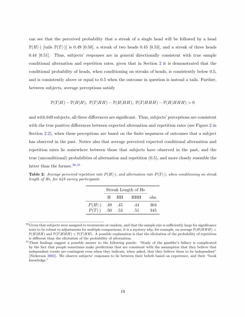
can see that the perceived probability that a streak of a single head will be followed by a head

P(H|·) [tails P(T |·)] is 0.49 [0.50], a streak of two heads 0.45 [0.53], and a streak of three heads

0.44 [0.51]. Thus, subjects’ responses are in general directionally consistent with true sample

conditional alternation and repetition rates, given that in Section 2 it is demonstrated that the

conditional probability of heads, when conditioning on streaks of heads, is consistently below 0.5,

and is consistently above or equal to 0.5 when the outcome in question is instead a tails. Further,

between subjects, average perceptions satisfy

P(T |H)− P(H|H), P(T |HH)− P(H|HH), P(T |HHH)− P(H|HHH) > 0

and with 649 subjects, all three differences are significant. Thus, subjects’ perceptions are consistent

with the true positive differences between expected alternation and repetition rates (see Figure 2 in

Section 2.2), when these perceptions are based on the finite sequences of outcomes that a subject

has observed in the past. Notice also that average perceived expected conditional alternation and

repetition rates lie somewhere between those that subjects have observed in the past, and the

true (unconditional) probabilities of alternation and repetition (0.5), and more closely resemble the

latter than the former.30,31

Table 2: Average perceived repetition rate P (H|·), and alternation rate P (T |·), when conditioning on streaklength of Hs, for 649 survey participants

Streak Length of Hs

H HH HHH obs.

P (H|·) .49 .45 .44 304P (T |·) .50 .53 .51 345

30Given that subjects were assigned to treatments at random, and that the sample size is sufficiently large for significancetests to be robust to adjustments for multiple comparisons, it is a mystery why, for example, on average P(H|HHH) <P(H|HH) and P(T |HHH) < P(T |HH). A possible explanation is that the elicitation of the probability of repetitionis different than the elicitation of the probability of alternation.

31These findings suggest a possible answer to the following puzzle: “Study of the gambler’s fallacy is complicatedby the fact that people sometimes make predictions that are consistent with the assumption that they believe thatindependent events are contingent even when they indicate, when asked, that they believe them to be independent”(Nickerson 2002). We observe subjects’ responses to lie between their beliefs based on experience, and their “bookknowledge.”

19

3.2 The Hot Hand Fallacy

This account explains both the formation and maintenance of the erroneous belief in

the hot hand: if random sequences are perceived as streak shooting, then no amount

of exposure to such sequences will convince the player, the coach, or the fan that the

sequences are in fact random.” (Gilovich et al. 1985)

The hot hand fallacy typically refers to the mistaken belief that success tends to follow success

(hot hand), when in fact observed successes are consistent with the typical fluctuations of a chance

process. The original evidence of the fallacy was provided by the seminal paper of Gilovich et al.

(1985), in which the authors found that basketball players’ beliefs that a player has “a better chance

of making a shot after having just made his last two or three shots than he does after having just

missed his last two or three shots” were not supported by the analysis of shooting data. Because

these players were experts who, despite the evidence, continued to make high-stakes decisions

based on their mistaken beliefs, the hot hand fallacy came to be characterized as a “massive and

widespread cognitive illusion” (Kahneman 2011).32 The strength of the original results has had a

large influence on empirical and theoretical work in areas related to decision making with sequential

data, both in economics and psychology.

In the Gilovich et al. (1985) study, and the other studies in basketball that follow, player

performance records – patterns in hits (successes) and misses (failures) – are checked to see if they

“differ from sequences of heads and tails produced by [weighted] coin tosses”(Gilovich et al. 1985).

The standard measure of hot hand effect size in these studies is to compare the empirical probability

of a hit on those shots that immediately follow a streak of hits to the empirical probability of a

hit on those shots that immediately follow a streak of misses, where a streak is typically defined

as a shot taken after 3, 4, 5, . . . hits in a row (Avugos, Bar-Eli, Ritov, and Sher 2013; Gilovich

et al. 1985; Koehler and Conley 2003).33 This comparison appears to be a sound one: if a player

32The fallacy view has been the consensus in the economics literature on sequential decision making, and the existenceof the fallacy itself has been highlighted in the general discourse as a salient example of how statistical analysis canreveal the flaws of expert intuition (e.g. see (Davidson 2013)).

33While defining the cutoff for a streak in this way agrees with the “rule of three” for human perception of streaks(Carlson and Shu 2007), when working with data, the choice of the cutoff involves a trade-off. The larger the cutoff k,the higher the probability that the player is actually hot on those shots that immediately follow these streaks, whichreduces measurement error. On the other hand, as k gets larger, fewer shots are available, which leads to a smallersample size and reduced statistical power (and a higher bias in the empirical probability). See Miller and Sanjurjo(2014) for a more thorough discussion, which explicitly considers a number of plausible hot hand models.

20

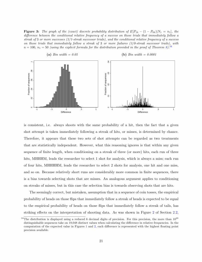
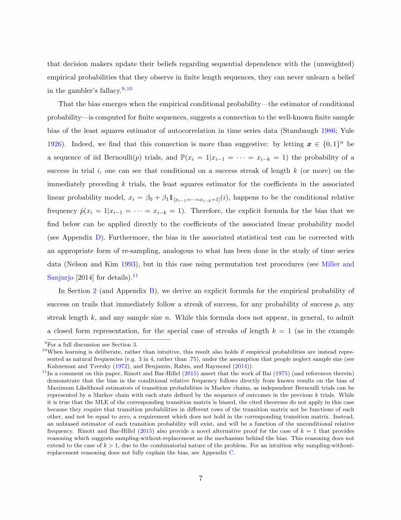
Figure 3: The graph of the (exact) discrete probability distribution of E[P1k − (1 − P0k)|N1 = n1], thedifference between the conditional relative frequency of a success on those trials that immediately follow astreak of 3 or more successes (3/1-streak successor trials), and the conditional relative frequency of a successon those trials that immediately follow a streak of 3 or more failures (3/0-streak successor trails), withn = 100, n1 = 50 (using the explicit formula for the distribution provided in the proof of Theorem 8).34

(a) Bin width = 0.05

0.0

2.0

4.0

6.0

8.1

Fra

ctio

n of

seq

uenc

es

-1 -.5 0 .5 1

Difference

(b) Bin width = 0.0001

0.0

1.0

2.0

3.0

4

Fra

ctio

n of

seq

uenc

es

-1 -.5 0 .5 1

Difference

is consistent, i.e. always shoots with the same probability of a hit, then the fact that a given

shot attempt is taken immediately following a streak of hits, or misses, is determined by chance.

Therefore, it appears that these two sets of shot attempts can be regarded as two treatments

that are statistically independent. However, what this reasoning ignores is that within any given

sequence of finite length, when conditioning on a streak of three (or more) hits, each run of three

hits, MHHHM, leads the researcher to select 1 shot for analysis, which is always a miss; each run

of four hits, MHHHHM, leads the researcher to select 2 shots for analysis, one hit and one miss,

and so on. Because relatively short runs are considerably more common in finite sequences, there

is a bias towards selecting shots that are misses. An analogous argument applies to conditioning

on streaks of misses, but in this case the selection bias is towards observing shots that are hits.

The seemingly correct, but mistaken, assumption that in a sequence of coin tosses, the empirical

probability of heads on those flips that immediately follow a streak of heads is expected to be equal

to the empirical probability of heads on those flips that immediately follow a streak of tails, has

striking effects on the interpretation of shooting data. As was shown in Figure 2 of Section 2.2,

34The distribution is displayed using a reduced 6 decimal digits of precision. For this precision, the more than 1029

distinguishable sequences take on 19,048 distinct values when calculating the difference in relative frequencies. In thecomputation of the expected value in Figures 1 and 2, each difference is represented with the highest floating pointprecision available.

21

the bias in this comparison between conditional relative frequencies is more than double that of

the comparison of either conditional relative frequency to the true probability (under the Bernoulli

assumption). If players were to shoot with a fixed hit rate (the null Bernoulli assumption), then,

given the parameters of the original study, one should in fact expect the difference in these relative

frequencies to be −0.08, rather than 0. Moreover, the distribution of the differences will have a

pronounced negative skew. In Figure 3 we present the exact distribution of the difference between

these conditional relative frequencies (for two different bin sizes), following Theorem 8 of Appendix

B. The distribution is generated using the target parameters of the original study: sequences of

length n = 100, n1 = 50 hits, and streaks of length k = 3 or more. As can be seen, the distribution

has a pronounced negative skew, with 63 percent of observations less than 0 (median = -.06).

The effects of this bias can be seen in Table 3, which reproduces data from Table 4 of Gilovich

et al. (1985). The table presents shooting performance records for each of the 14 male and 12 female

Cornell University basketball players who participated in the controlled shooting experiment of the

original hot hand study (Gilovich et al. 1985). One can see the number of shots taken, overall

field goal percentage, relative frequency of a hit on those shots that immediately follow a streak

of three (or more) hits, p(hit|3 hits), relative frequency of a hit on those shots that immediately

follow a streak of three (or more) misses, p(hit|3 misses), and the expected difference between these

quantities. Under the incorrect assumption that these conditional relative frequencies are expected

to be equal to each player’s overall field goal percentage, it indeed appears as if there is little to

no evidence of hot hand shooting. Likewise, under the incorrect assumption that the difference

between these two conditional relative frequencies is expected to be zero, the difference of +0.03

may seem like directional evidence of a slight hot hand, but it is not statistically significant.35

The last column corrects for the incorrect assumption by subtracting from each player’s observed

difference the actual expected difference under the null hypothesis that the player shoots with a

constant probability of a hit, given his/her overall field goal percentage (see the end of the section

for more on the bias correction). Once this bias correction is made, one can see that 19 of the

25 players directionally exhibit hot hand shooting, and that the average difference in shooting

35A common criticism of the original study, as well as subsequent studies, is that they are under-powered, thus evensubstantial differences are not registered as significant (see Miller and Sanjurjo (2014) for a power analysis, and acomplete discussion of the previous literature).

22

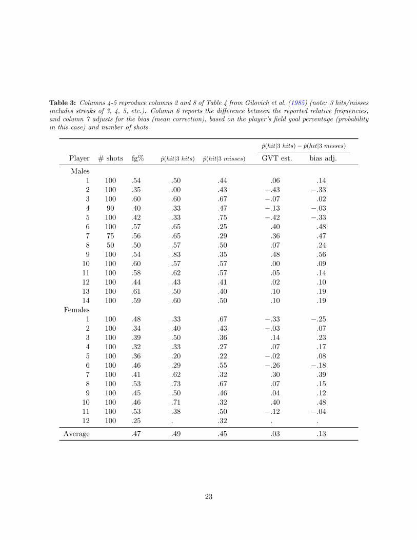
Table 3: Columns 4-5 reproduce columns 2 and 8 of Table 4 from Gilovich et al. (1985) (note: 3 hits/missesincludes streaks of 3, 4, 5, etc.). Column 6 reports the difference between the reported relative frequencies,and column 7 adjusts for the bias (mean correction), based on the player’s field goal percentage (probabilityin this case) and number of shots.

p(hit|3 hits)− p(hit|3 misses)

Player # shots fg% p(hit|3 hits) p(hit|3 misses) GVT est. bias adj.

Males1 100 .54 .50 .44 .06 .142 100 .35 .00 .43 −.43 −.333 100 .60 .60 .67 −.07 .024 90 .40 .33 .47 −.13 −.035 100 .42 .33 .75 −.42 −.336 100 .57 .65 .25 .40 .487 75 .56 .65 .29 .36 .478 50 .50 .57 .50 .07 .249 100 .54 .83 .35 .48 .56

10 100 .60 .57 .57 .00 .0911 100 .58 .62 .57 .05 .1412 100 .44 .43 .41 .02 .1013 100 .61 .50 .40 .10 .1914 100 .59 .60 .50 .10 .19

Females1 100 .48 .33 .67 −.33 −.252 100 .34 .40 .43 −.03 .073 100 .39 .50 .36 .14 .234 100 .32 .33 .27 .07 .175 100 .36 .20 .22 −.02 .086 100 .46 .29 .55 −.26 −.187 100 .41 .62 .32 .30 .398 100 .53 .73 .67 .07 .159 100 .45 .50 .46 .04 .12

10 100 .46 .71 .32 .40 .4811 100 .53 .38 .50 −.12 −.0412 100 .25 . .32 . .

Average .47 .49 .45 .03 .13

23

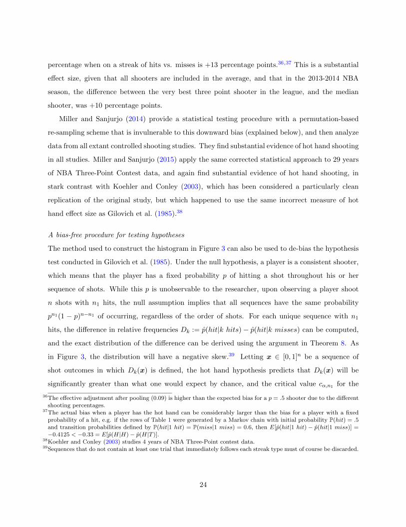
percentage when on a streak of hits vs. misses is +13 percentage points.36,37 This is a substantial

effect size, given that all shooters are included in the average, and that in the 2013-2014 NBA

season, the difference between the very best three point shooter in the league, and the median

shooter, was +10 percentage points.

Miller and Sanjurjo (2014) provide a statistical testing procedure with a permutation-based

re-sampling scheme that is invulnerable to this downward bias (explained below), and then analyze

data from all extant controlled shooting studies. They find substantial evidence of hot hand shooting

in all studies. Miller and Sanjurjo (2015) apply the same corrected statistical approach to 29 years

of NBA Three-Point Contest data, and again find substantial evidence of hot hand shooting, in

stark contrast with Koehler and Conley (2003), which has been considered a particularly clean

replication of the original study, but which happened to use the same incorrect measure of hot

hand effect size as Gilovich et al. (1985).38

A bias-free procedure for testing hypotheses

The method used to construct the histogram in Figure 3 can also be used to de-bias the hypothesis

test conducted in Gilovich et al. (1985). Under the null hypothesis, a player is a consistent shooter,

which means that the player has a fixed probability p of hitting a shot throughout his or her

sequence of shots. While this p is unobservable to the researcher, upon observing a player shoot

n shots with n1 hits, the null assumption implies that all sequences have the same probability

pn1(1 − p)n−n1 of occurring, regardless of the order of shots. For each unique sequence with n1

hits, the difference in relative frequencies Dk := p(hit|k hits)− p(hit|k misses) can be computed,

and the exact distribution of the difference can be derived using the argument in Theorem 8. As

in Figure 3, the distribution will have a negative skew.39 Letting x ∈ [0, 1]n be a sequence of

shot outcomes in which Dk(x) is defined, the hot hand hypothesis predicts that Dk(x) will be

significantly greater than what one would expect by chance, and the critical value cα,n1 for the

36The effective adjustment after pooling (0.09) is higher than the expected bias for a p = .5 shooter due to the differentshooting percentages.

37The actual bias when a player has the hot hand can be considerably larger than the bias for a player with a fixedprobability of a hit, e.g. if the rows of Table 1 were generated by a Markov chain with initial probability P(hit) = .5and transition probabilities defined by P(hit|1 hit) = P(miss|1 miss) = 0.6, then E[p(hit|1 hit) − p(hit|1 miss)] =−0.4125 < −0.33 = E[p(H|H)− p(H|T )].

38Koehler and Conley (2003) studies 4 years of NBA Three-Point contest data.39Sequences that do not contain at least one trial that immediately follows each streak type must of course be discarded.

24

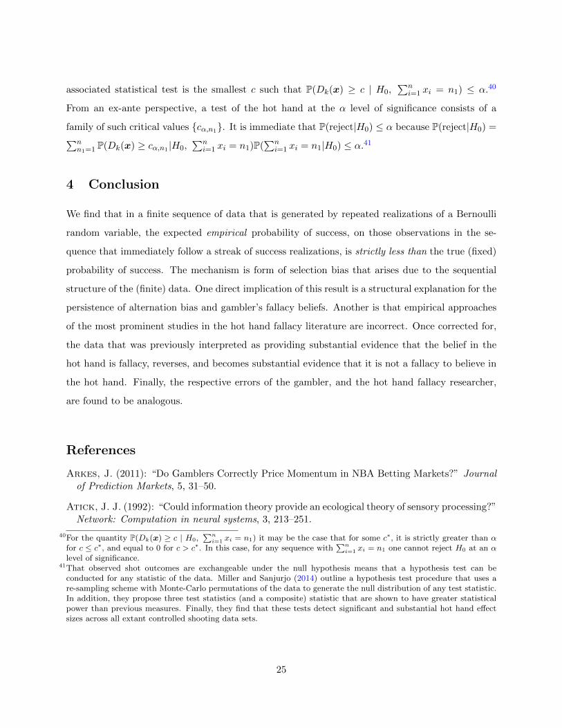
associated statistical test is the smallest c such that P(Dk(x) ≥ c | H0,∑n

i=1 xi = n1) ≤ α.40

From an ex-ante perspective, a test of the hot hand at the α level of significance consists of a

family of such critical values {cα,n1}. It is immediate that P(reject|H0) ≤ α because P(reject|H0) =∑nn1=1 P(Dk(x) ≥ cα,n1 |H0,

∑ni=1 xi = n1)P(

∑ni=1 xi = n1|H0) ≤ α.41

4 Conclusion

We find that in a finite sequence of data that is generated by repeated realizations of a Bernoulli

random variable, the expected empirical probability of success, on those observations in the se-

quence that immediately follow a streak of success realizations, is strictly less than the true (fixed)

probability of success. The mechanism is form of selection bias that arises due to the sequential

structure of the (finite) data. One direct implication of this result is a structural explanation for the

persistence of alternation bias and gambler’s fallacy beliefs. Another is that empirical approaches

of the most prominent studies in the hot hand fallacy literature are incorrect. Once corrected for,

the data that was previously interpreted as providing substantial evidence that the belief in the

hot hand is fallacy, reverses, and becomes substantial evidence that it is not a fallacy to believe in

the hot hand. Finally, the respective errors of the gambler, and the hot hand fallacy researcher,

are found to be analogous.

References

Arkes, J. (2011): “Do Gamblers Correctly Price Momentum in NBA Betting Markets?” Journalof Prediction Markets, 5, 31–50.

Atick, J. J. (1992): “Could information theory provide an ecological theory of sensory processing?”Network: Computation in neural systems, 3, 213–251.

40For the quantity P(Dk(x) ≥ c | H0,∑ni=1 xi = n1) it may be the case that for some c∗, it is strictly greater than α

for c ≤ c∗, and equal to 0 for c > c∗. In this case, for any sequence with∑ni=1 xi = n1 one cannot reject H0 at an α

level of significance.41That observed shot outcomes are exchangeable under the null hypothesis means that a hypothesis test can be

conducted for any statistic of the data. Miller and Sanjurjo (2014) outline a hypothesis test procedure that uses are-sampling scheme with Monte-Carlo permutations of the data to generate the null distribution of any test statistic.In addition, they propose three test statistics (and a composite) statistic that are shown to have greater statisticalpower than previous measures. Finally, they find that these tests detect significant and substantial hot hand effectsizes across all extant controlled shooting data sets.

25

Avery, C. and J. Chevalier (1999): “Identifying Investor Sentiment from Price Paths: TheCase of Football Betting,” Journal of Business, 72, 493–521.

Avugos, S., M. Bar-Eli, I. Ritov, and E. Sher (2013): “The elusive reality of efficacy perfor-mance cycles in basketball shooting: analysis of players performance under invariant conditions,”International Journal of Sport and Exercise Psychology, 11, 184–202.

Bai, D. S. (1975): “Efficient Estimation of Transition Probabilities in a Markov Chain,” TheAnnals of Statistics, 3, 1305–1317.

Bar-Hillel, M. and W. A. Wagenaar (1991): “The perception of randomness,” Advances inApplied Mathematics, 12, 428–454.

Barberis, N. and R. Thaler (2003): “A survey of behavioral finance,” Handbook of the Eco-nomics of Finance, 1, 1053–1128.

Benjamin, D. J., M. Rabin, and C. Raymond (2014): “A Model of Non-Belief in the Law ofLarge Numbers,” Working Paper.

Brown, W. A. and R. D. Sauer (1993): “Does the Basketball Market Believe in the Hot Hand?Comment,” American Economic Review, 83, 1377–1386.

Budescu, D. V. and A. Rapoport (1994): “Subjective randomization in one-and two-persongames,” Journal of Behavioral Decision Making, 7, 261–278.

Camerer, C. F. (1989): “Does the Basketball Market Believe in the ’Hot Hand,’?” AmericanEconomic Review, 79, 1257–1261.

Carlson, K. A. and S. B. Shu (2007): “The rule of three: how the third event signals theemergence of a streak,” Organizational Behavior and Human Decision Processes, 104, 113–121.

Cowan, N. (2001): “The magical number 4 in short-term memory: A reconsideration of mentalstorage capacity,” Behavioral and Brain Sciences, 24, 87–114.

Croson, R. and J. Sundali (2005): “The Gamblers Fallacy and the Hot Hand: Empirical Datafrom Casinos,” Journal of Risk and Uncertainty, 30, 195–209.

Davidson, A. (2013): “Boom, Bust or What?” New York Times.

De Bondt, W. P. (1993): “Betting on trends: Intuitive forecasts of financial risk and return,”International Journal of Forecasting, 9, 355–371.

De Long, J. B., A. Shleifer, L. H. Summers, and R. J. Waldmann (1991): “The Survivalof Noise Traders In Financial-markets,” Journal of Business, 64, 1–19.

Durham, G. R., M. G. Hertzel, and J. S. Martin (2005): “The Market Impact of Trendsand Sequences in Performance: New Evidence,” Journal of Finance, 60, 2551–2569.

Feller, W. (1968): An Introduction to Probability Theory and Its Applications, New York: JohnWiley & Sons.

26

Galbo-Jørgensen, C. B., S. Suetens, and J.-R. Tyran (2015): “Predicting Lotto NumbersA natural experiment on the gamblers fallacy and the hot hand fallacy,” Journal of the EuropeanEconomic Association, forthcoming, working Paper.

Gilovich, T., R. Vallone, and A. Tversky (1985): “The Hot Hand in Basketball: On theMisperception of Random Sequences,” Cognitive Psychology, 17, 295–314.

Guryan, J. and M. S. Kearney (2008): “Gambling at Lucky Stores: Empirical Evidence fromState Lottery Sales,” American Economic Review, 98, 458–473.

Hogarth, R. M. (2010): “Intuition: A Challenge for Psychological Research on Decision Making,”Psychological Inquiry, 21, 338–353.

Kahneman, D. (2011): Thinking, Fast and Slow, Farrar, Straus and Giroux.

Kahneman, D. and M. W. Riepe (1998): “Aspects of Investor Psychology: Beliefs, preferences,and biases investment advisors should know about,” Journal of Portfolio Management, 24, 1–21.

Kahneman, D. and A. Tversky (1972): “Subjective Probability: A Judgement of Representa-tiveness,” Cognitive Psychology, 3, 430–454.

Kareev, Y. (1992): “Not that bad after all: Generation of random sequences.” Journal of Exper-imental Psychology: Human Perception and Performance, 18, 1189–1194.

——— (2000): “Seven (indeed, plus or minus two) and the detection of correlations.” PsychologicalReview, 107, 397–402.

Koehler, J. J. and C. A. Conley (2003): “The “hot hand” myth in professional basketball,”Journal of Sport and Exercise Psychology, 25, 253–259.

Lee, M. and G. Smith (2002): “Regression to the mean and football wagers,” Journal of Behav-ioral Decision Making, 15, 329–342.

Loh, R. K. and M. Warachka (2012): “Streaks in Earnings Surprises and the Cross-Section ofStock Returns,” Management Science, 58, 1305–1321.

Lopes, L. L. and G. C. Oden (1987): “Distinguishing between random and nonrandom events,”Journal of Experimental Psychology: Learning, Memory, and Cognition, 13, 392–400.

Malkiel, B. G. (2011): A random walk down Wall Street: the time-tested strategy for sucessfulinvesting, New York: W. W. Norton & Company.

Miller, G. A. (1956): “The magical number seven, plus or minus two: Some limits on our capacityfor processing information.” Psychological Review, 63, 81–97.

Miller, J. B. and A. Sanjurjo (2014): “A Cold Shower for the Hot Hand Fallacy,” WorkingPaper.

——— (2015): “Is the Belief in the Hot Hand a Fallacy in the NBA Three Point Shootout?”Working Paper.

27

Narayanan, S. and P. Manchanda (2012): “An empirical analysis of individual level casinogambling behavior,” Quantitative Marketing and Economics, 10, 27–62.

Nelson, C. R. and M. J. Kim (1993): “Predictable Stock Returns: The Role of Small SampleBias,” Journal of Finance, 48, 641–661.

Neuringer, A. (1986): “Can people behave “randomly?”: The role of feedback.” Journal ofExperimental Psychology: General, 115, 62.

Nickerson, R. S. (2002): “The production and perception of randomness,” Psychological Review,109, 350–357.

Oskarsson, A. T., L. V. Boven, G. H. McClelland, and R. Hastie (2009): “What’s next?Judging sequences of binary events,” Psychological Bulletin, 135, 262–385.

Paul, R. J. and A. P. Weinbach (2005): “Bettor Misperceptions in the NBA: The Overbettingof Large Favorites and the ‘Hot Hand’,” Journal of Sports Economics, 6, 390–400.

Rabin, M. (2002): “Inference by Believers in the Law of Small Numbers,” Quarterly Journal ofEconomics, 117, 775–816.

Rabin, M. and D. Vayanos (2010): “The Gamblers and Hot-Hand Fallacies: Theory and Appli-cations,” Review of Economic Studies, 77, 730–778.

Rapoport, A. and D. V. Budescu (1992): “Generation of random series in two-person strictlycompetitive games.” Journal of Experimental Psychology: General, 121, 352–.

Rinott, Y. and M. Bar-Hillel (2015): “Comments on a ’Hot Hand’ Paper by Miller and San-jurjo,” Federmann Center For The Study Of Rationality, The Hebrew University Of Jerusalem.Discussion Paper # 688 (August 11).

Riordan, J. (1958): An Introduction to Combinatorial Analysis, New York: John Wiley & Sons.

Simoncelli, E. P. and B. A. Olshausen (2001): “Natural Image Statistics And Neural Repre-sentation,” Annual Review of Neuroscience, 24, 1193–1216.

Sinkey, M. and T. Logan (2013): “Does the Hot Hand Drive the Market?” Eastern EconomicJournal, Advance online publication, doi:10.1057/eej.2013.33.

Smith, G., M. Levere, and R. Kurtzman (2009): “Poker Player Behavior After Big Wins andBig Losses,” Management Science, 55, 1547–1555.

Stambaugh, R. F. (1986): “Bias in Regressions with lagged Stochastic Regressors,” WorkingPaper No. 156.

——— (1999): “Predictive regressions,” Journal of Financial Economics, 54, 375–421.

Sundali, J. and R. Croson (2006): “Biases in casino betting: The hot and the gamblers fallacy,”Judgement and Decision Making, 1, 1–12.

Xu, J. and N. Harvey (2014): “Carry on winning: The gambler’s fallacy creates hot hand effectsin online gambling,” Cognition, 131, 173 – 180.

28

Yuan, J., G.-Z. Sun, and R. Siu (2014): “The Lure of Illusory Luck: How Much Are PeopleWilling to Pay for Random Shocks,” Journal of Economic Behavior & Organization, forthcoming.

Yule, G. U. (1926): “Why do we Sometimes get Nonsense-Correlations between Time-Series?–AStudy in Sampling and the Nature of Time-Series,” Journal of the Royal Statistical Society, 89,1–63.

29

A Appendix: Section 2 Proofs

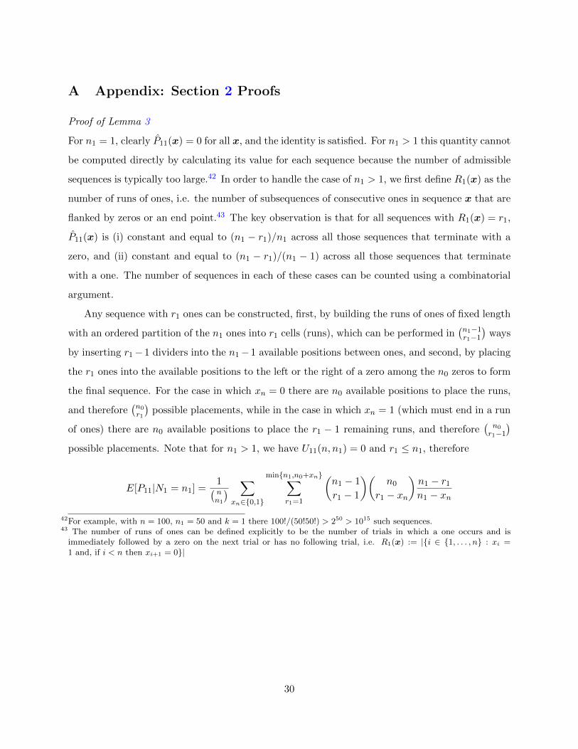
Proof of Lemma 3

For n1 = 1, clearly P11(x) = 0 for all x, and the identity is satisfied. For n1 > 1 this quantity cannot

be computed directly by calculating its value for each sequence because the number of admissible

sequences is typically too large.42 In order to handle the case of n1 > 1, we first define R1(x) as the

number of runs of ones, i.e. the number of subsequences of consecutive ones in sequence x that are

flanked by zeros or an end point.43 The key observation is that for all sequences with R1(x) = r1,

P11(x) is (i) constant and equal to (n1 − r1)/n1 across all those sequences that terminate with a

zero, and (ii) constant and equal to (n1 − r1)/(n1 − 1) across all those sequences that terminate

with a one. The number of sequences in each of these cases can be counted using a combinatorial

argument.

Any sequence with r1 ones can be constructed, first, by building the runs of ones of fixed length

with an ordered partition of the n1 ones into r1 cells (runs), which can be performed in(n1−1r1−1

)ways

by inserting r1−1 dividers into the n1−1 available positions between ones, and second, by placing

the r1 ones into the available positions to the left or the right of a zero among the n0 zeros to form

the final sequence. For the case in which xn = 0 there are n0 available positions to place the runs,

and therefore(n0

r1

)possible placements, while in the case in which xn = 1 (which must end in a run

of ones) there are n0 available positions to place the r1 − 1 remaining runs, and therefore(n0

r1−1

)possible placements. Note that for n1 > 1, we have U11(n, n1) = 0 and r1 ≤ n1, therefore

E[P11|N1 = n1] =1(nn1

) ∑xn∈{0,1}

min{n1,n0+xn}∑r1=1

(n1 − 1

r1 − 1

)(n0

r1 − xn

)n1 − r1

n1 − xn

42For example, with n = 100, n1 = 50 and k = 1 there 100!/(50!50!) > 250 > 1015 such sequences.43 The number of runs of ones can be defined explicitly to be the number of trials in which a one occurs and is

immediately followed by a zero on the next trial or has no following trial, i.e. R1(x) := |{i ∈ {1, . . . , n} : xi =1 and, if i < n then xi+1 = 0}|

30

For the case in which xn = 0, the inner sum satisfies:

min{n1,n0}∑r1=1

(n1 − 1

r1 − 1

)(n0

r1

)n1 − r1

n1=

min{n1,n0}∑r1=1

(n1 − 1

r1 − 1

)(n0

r1

)(1− r1

n1

)

=

(n− 1

n0 − 1

)− 1

n1

min{n1,n0}∑r1=1

(n1 − 1

r1 − 1

)(n0

r1

)r1

=

(n− 1

n0 − 1

)− n0

n1

min{n1,n0}∑r1=1

(n1 − 1

r1 − 1

)(n0 − 1

r1 − 1

)

=

(n− 1

n0 − 1

)− n0

n1

min{n1−1,n0−1}∑x=0

(n1 − 1

x

)(n0 − 1

x

)=

(n− 1

n0 − 1

)− n0

n1

(n− 2

n1 − 1

)

The left term of the second line follows because it is the total number of sequences that can be

formed in the first n − 1 positions with n0 − 1 zeros and n1 = n − n0 ones. The final line follows

from an application of Vandermonde’s convolution.44

For the case in which xn = 1, the inner sum can be reduced using similar arguments:

44 Vandermonde’s convolution is given as

min{r−m,n}∑k=max{−m,n−s}

(r

m+ k

)(s

n− k

)=

(r + s

m+ n

)

from which one can derive the following identity, which we apply

min{`−m,s−n}∑k=max{−m,−n}

(`

m+ k

)(s

n+ k

)=

min{`−m,s−n}∑k=max{−m,−n}

(s

n+ k

)(`

(`−m)− k

)=

(`+ s

`−m+ n

)

31

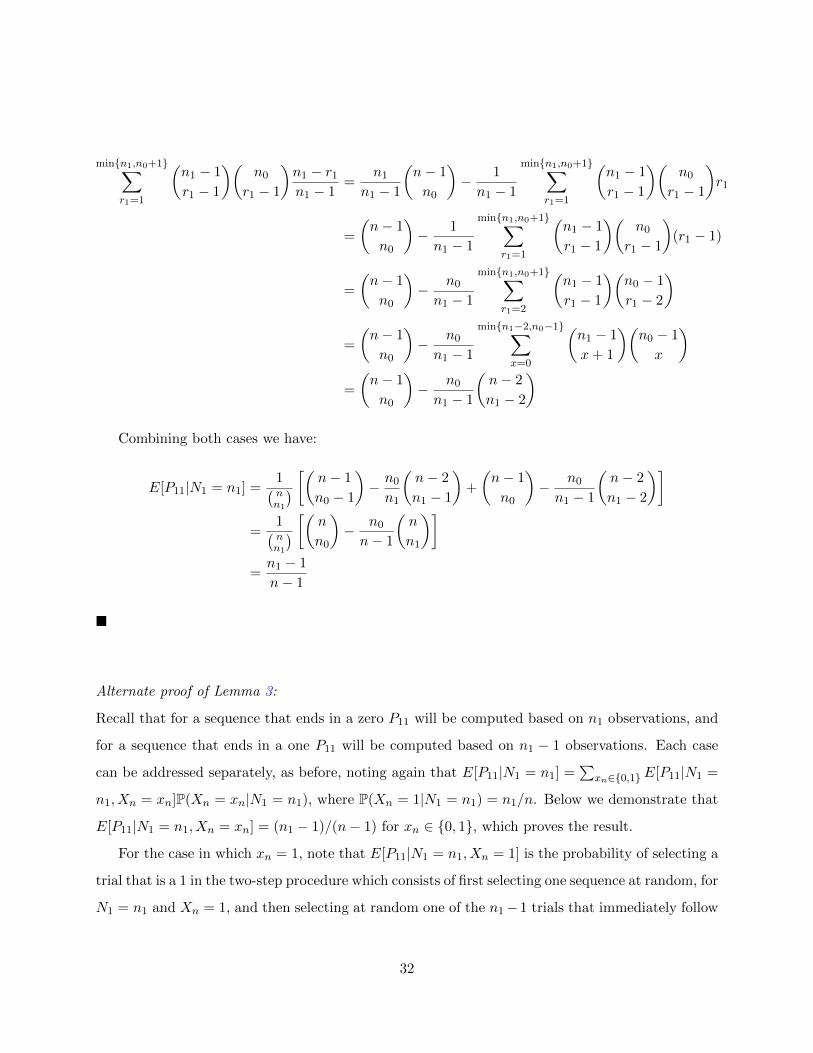
min{n1,n0+1}∑r1=1

(n1 − 1

r1 − 1

)(n0

r1 − 1

)n1 − r1

n1 − 1=

n1

n1 − 1

(n− 1

n0

)− 1

n1 − 1

min{n1,n0+1}∑r1=1

(n1 − 1

r1 − 1

)(n0

r1 − 1

)r1

=

(n− 1

n0

)− 1

n1 − 1

min{n1,n0+1}∑r1=1

(n1 − 1

r1 − 1

)(n0

r1 − 1

)(r1 − 1)

=

(n− 1

n0

)− n0

n1 − 1

min{n1,n0+1}∑r1=2

(n1 − 1

r1 − 1

)(n0 − 1

r1 − 2

)

=

(n− 1

n0

)− n0

n1 − 1

min{n1−2,n0−1}∑x=0

(n1 − 1

x+ 1

)(n0 − 1

x

)=

(n− 1

n0

)− n0

n1 − 1

(n− 2

n1 − 2

)

Combining both cases we have:

E[P11|N1 = n1] =1(nn1

) [( n− 1

n0 − 1

)− n0

n1

(n− 2

n1 − 1

)+

(n− 1

n0

)− n0

n1 − 1

(n− 2

n1 − 2

)]=

1(nn1

) [( nn0

)− n0

n− 1

(n

n1

)]=n1 − 1

n− 1

�

Alternate proof of Lemma 3:

Recall that for a sequence that ends in a zero P11 will be computed based on n1 observations, and

for a sequence that ends in a one P11 will be computed based on n1 − 1 observations. Each case

can be addressed separately, as before, noting again that E[P11|N1 = n1] =∑

xn∈{0,1}E[P11|N1 =

n1, Xn = xn]P(Xn = xn|N1 = n1), where P(Xn = 1|N1 = n1) = n1/n. Below we demonstrate that

E[P11|N1 = n1, Xn = xn] = (n1 − 1)/(n− 1) for xn ∈ {0, 1}, which proves the result.

For the case in which xn = 1, note that E[P11|N1 = n1, Xn = 1] is the probability of selecting a

trial that is a 1 in the two-step procedure which consists of first selecting one sequence at random, for

N1 = n1 and Xn = 1, and then selecting at random one of the n1−1 trials that immediately follow

32

a 1, and observing the outcome. Because each sequence with N1 = n1 and Xn = 1 contributes the

same number of trial observations (n1 − 1) to the computation of P11, this procedure is equivalent

to selecting one trial at random from the(n−1n1−1

)(n1 − 1) trials that immediately follow a 1 (across

all sequences with N1 = n1 and Xn = 1). It is equiprobable that the selected trial be located in any

of the positions from 2 to n. If the trial is located in one of the positions from 2 to n−1, then there

are n1−2 1s available (having removed the 1s from the selected trial and the end point) among the

n− 2 trials available, and therefore the probability that the trial is a 1 is equal to (n1− 2)/(n− 2).

On the other hand, if the trial is located in position n, then the trial must be a 1. Therefore

E[P11|N1 = n1, Xn = 1] = (n− 2)[(n1 − 2)/(n− 2)][1/(n− 1)] + 1/(n− 1) = (n1 − 1)/(n− 1).

For the case in which xn = 0, analogous to the previous argument, E[P11|N1 = n1, Xn = 0]

is the probability of selecting a trial that is a 1 in the procedure of selecting one trial at ran-

dom from the(n−1n1

)n1 trials that immediately follow a 1 (across all sequences with N1 = n1

and Xn = 0). As before, it is equiprobable that the selected trial be located in any of the po-

sitions from 2 to n. If the trial is located in one of the positions from 2 to n − 1, then there

are n1 − 1 1s available (having removed the 1 from the selected trial) among the n − 2 tri-

als available, and therefore the probability that the trial is a 1 is equal to (n1 − 1)/(n − 2).

On the other hand, if the trial is located in position n, then the trial must be a 0. Therefore

E[P11|N1 = n1, Xn = 0] = (n−2)[(n1−1)/(n−2)][1/(n−1)] = (n1−1)/(n−1) = (n1−1)/(n−1).

�

Proof of Lemma 4

The full derivation of Equation 3 is as follows.

E[P11] = Cn∑

n1=1

pn1(1− p)n−n1

[(n

n1

)− U11(n, n1)

]· E[P11|N1 = n1]

=

∑nn1=2

(nn1

)pn1(1− p)n−n1 n1−1

n−1

1− (1− p)n − p(1− p)n−1

=1

n−1

[(np− np(1− p)n−1

)−(1− (1− p)n − np(1− p)n−1

)]1− (1− p)n − p(1− p)n−1

=

[p− 1−(1−p)n

n

]nn−1

1− (1− p)n − p(1− p)n−1

33

where the second line follows because U11(n, n1) = 0 for n1 > 1 and C = 1/[1−(1−p)n−p(1−p)n−1].

Clearly E[P11] < p.

�

Proof of Lemma 5

We show that for n > 2 and n1 = 1, . . . , n− 1,

E[D1|N1 = n1] = − 1

n− 1

If 1 < n1 < n− 1 then D1 = P11 − (1− P01) is defined for all sequences. Therefore, by linearity of

the expectation, and Lemma 3, we have:

E[D1|N1 = n1] =E[P11|N1 = n1]− E[(1− P01|N1 = n1]

=n1 − 1

n− 1−(

1− n0 − 1

n− 1

)=− 1

n− 1

If n1 = 1 then there are n− 1 possible sequences in which D1 is defined (i.e. with 1 not in the final

position). For the sequence in which 1 is in the first position, D1 = 0. For the other n−2 sequences,

D1 = −1/(n− 2). Therefore, E[D1|N1 = 1] = −1/(n− 1). The argument for n1 = n− 1 is analo-

gous, with D1 undefined for the sequence in which there is a 0 in the last position, equal to 0 for

the sequence in which there is 0 in the first position, and equal to −1/(n−2) for all other sequences.

That the conditional expectation is independent of N1 implies that E[D1] is independent of p,

and we have the result.

�

34

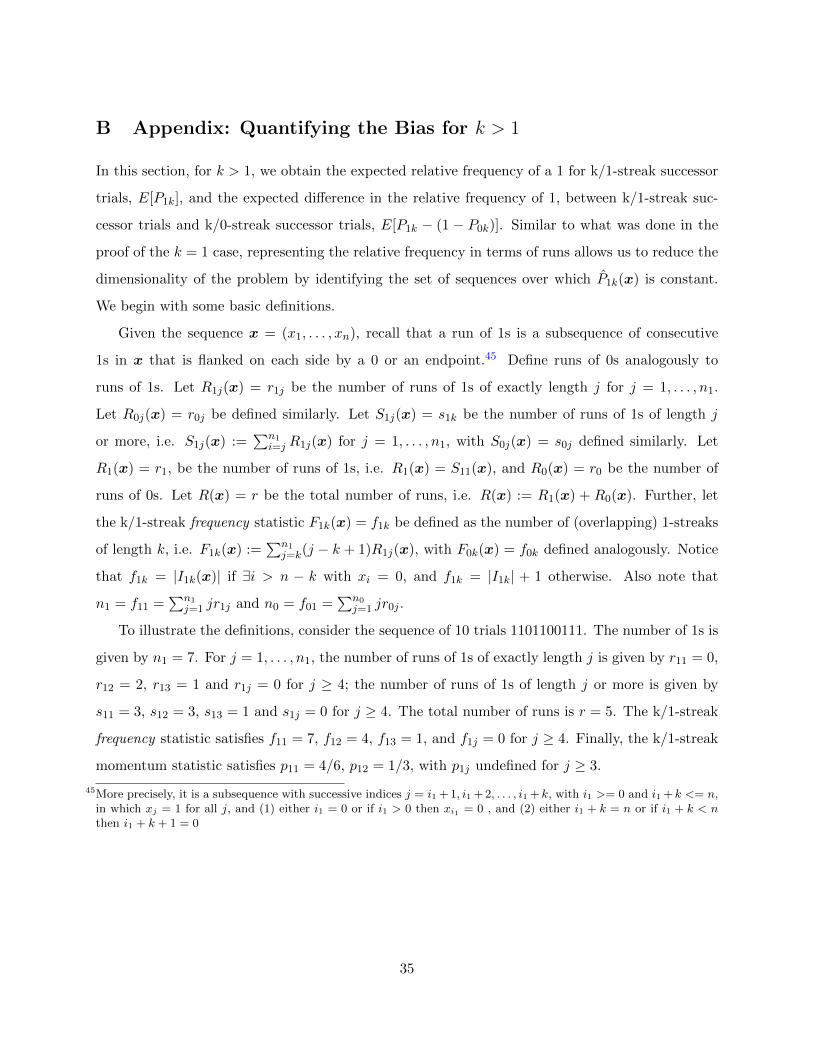
B Appendix: Quantifying the Bias for k > 1

In this section, for k > 1, we obtain the expected relative frequency of a 1 for k/1-streak successor

trials, E[P1k], and the expected difference in the relative frequency of 1, between k/1-streak suc-

cessor trials and k/0-streak successor trials, E[P1k − (1 − P0k)]. Similar to what was done in the

proof of the k = 1 case, representing the relative frequency in terms of runs allows us to reduce the

dimensionality of the problem by identifying the set of sequences over which P1k(x) is constant.

We begin with some basic definitions.

Given the sequence x = (x1, . . . , xn), recall that a run of 1s is a subsequence of consecutive

1s in x that is flanked on each side by a 0 or an endpoint.45 Define runs of 0s analogously to

runs of 1s. Let R1j(x) = r1j be the number of runs of 1s of exactly length j for j = 1, . . . , n1.

Let R0j(x) = r0j be defined similarly. Let S1j(x) = s1k be the number of runs of 1s of length j

or more, i.e. S1j(x) :=∑n1

i=j R1j(x) for j = 1, . . . , n1, with S0j(x) = s0j defined similarly. Let

R1(x) = r1, be the number of runs of 1s, i.e. R1(x) = S11(x), and R0(x) = r0 be the number of

runs of 0s. Let R(x) = r be the total number of runs, i.e. R(x) := R1(x) + R0(x). Further, let

the k/1-streak frequency statistic F1k(x) = f1k be defined as the number of (overlapping) 1-streaks

of length k, i.e. F1k(x) :=∑n1

j=k(j − k + 1)R1j(x), with F0k(x) = f0k defined analogously. Notice

that f1k = |I1k(x)| if ∃i > n − k with xi = 0, and f1k = |I1k| + 1 otherwise. Also note that

n1 = f11 =∑n1

j=1 jr1j and n0 = f01 =∑n0

j=1 jr0j .

To illustrate the definitions, consider the sequence of 10 trials 1101100111. The number of 1s is

given by n1 = 7. For j = 1, . . . , n1, the number of runs of 1s of exactly length j is given by r11 = 0,

r12 = 2, r13 = 1 and r1j = 0 for j ≥ 4; the number of runs of 1s of length j or more is given by

s11 = 3, s12 = 3, s13 = 1 and s1j = 0 for j ≥ 4. The total number of runs is r = 5. The k/1-streak

frequency statistic satisfies f11 = 7, f12 = 4, f13 = 1, and f1j = 0 for j ≥ 4. Finally, the k/1-streak

momentum statistic satisfies p11 = 4/6, p12 = 1/3, with p1j undefined for j ≥ 3.

45More precisely, it is a subsequence with successive indices j = i1 + 1, i1 + 2, . . . , i1 +k, with i1 >= 0 and i1 +k <= n,in which xj = 1 for all j, and (1) either i1 = 0 or if i1 > 0 then xi1 = 0 , and (2) either i1 + k = n or if i1 + k < nthen i1 + k + 1 = 0

35

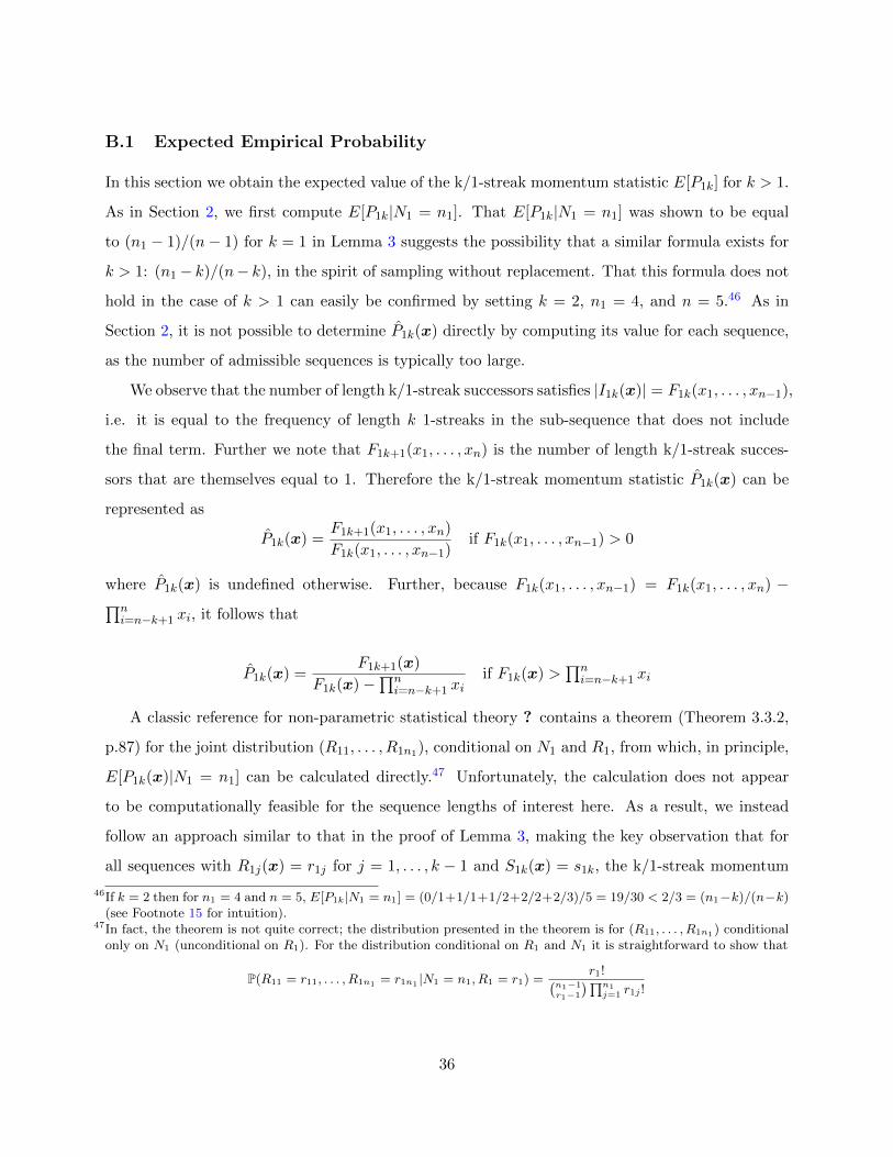
B.1 Expected Empirical Probability

In this section we obtain the expected value of the k/1-streak momentum statistic E[P1k] for k > 1.

As in Section 2, we first compute E[P1k|N1 = n1]. That E[P1k|N1 = n1] was shown to be equal

to (n1 − 1)/(n− 1) for k = 1 in Lemma 3 suggests the possibility that a similar formula exists for

k > 1: (n1− k)/(n− k), in the spirit of sampling without replacement. That this formula does not

hold in the case of k > 1 can easily be confirmed by setting k = 2, n1 = 4, and n = 5.46 As in

Section 2, it is not possible to determine P1k(x) directly by computing its value for each sequence,

as the number of admissible sequences is typically too large.

We observe that the number of length k/1-streak successors satisfies |I1k(x)| = F1k(x1, . . . , xn−1),

i.e. it is equal to the frequency of length k 1-streaks in the sub-sequence that does not include

the final term. Further we note that F1k+1(x1, . . . , xn) is the number of length k/1-streak succes-

sors that are themselves equal to 1. Therefore the k/1-streak momentum statistic P1k(x) can be

represented as

P1k(x) =F1k+1(x1, . . . , xn)

F1k(x1, . . . , xn−1)if F1k(x1, . . . , xn−1) > 0

where P1k(x) is undefined otherwise. Further, because F1k(x1, . . . , xn−1) = F1k(x1, . . . , xn) −∏ni=n−k+1 xi, it follows that

P1k(x) =F1k+1(x)

F1k(x)−∏ni=n−k+1 xi

if F1k(x) >∏ni=n−k+1 xi

A classic reference for non-parametric statistical theory ? contains a theorem (Theorem 3.3.2,

p.87) for the joint distribution (R11, . . . , R1n1), conditional on N1 and R1, from which, in principle,

E[P1k(x)|N1 = n1] can be calculated directly.47 Unfortunately, the calculation does not appear

to be computationally feasible for the sequence lengths of interest here. As a result, we instead

follow an approach similar to that in the proof of Lemma 3, making the key observation that for

all sequences with R1j(x) = r1j for j = 1, . . . , k − 1 and S1k(x) = s1k, the k/1-streak momentum

46If k = 2 then for n1 = 4 and n = 5, E[P1k|N1 = n1] = (0/1+1/1+1/2+2/2+2/3)/5 = 19/30 < 2/3 = (n1−k)/(n−k)(see Footnote 15 for intuition).

47In fact, the theorem is not quite correct; the distribution presented in the theorem is for (R11, . . . , R1n1) conditionalonly on N1 (unconditional on R1). For the distribution conditional on R1 and N1 it is straightforward to show that

P(R11 = r11, . . . , R1n1 = r1n1 |N1 = n1, R1 = r1) =r1!(

n1−1r1−1

)∏n1j=1 r1j !

36

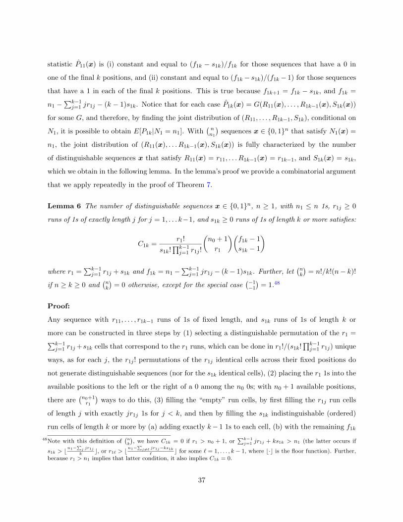
statistic P11(x) is (i) constant and equal to (f1k − s1k)/f1k for those sequences that have a 0 in

one of the final k positions, and (ii) constant and equal to (f1k − s1k)/(f1k − 1) for those sequences

that have a 1 in each of the final k positions. This is true because f1k+1 = f1k − s1k, and f1k =

n1 −∑k−1

j=1 jr1j − (k − 1)s1k. Notice that for each case P1k(x) = G(R11(x), . . . , R1k−1(x), S1k(x))

for some G, and therefore, by finding the joint distribution of (R11, . . . , R1k−1, S1k), conditional on

N1, it is possible to obtain E[P1k|N1 = n1]. With(nn1

)sequences x ∈ {0, 1}n that satisfy N1(x) =

n1, the joint distribution of (R11(x), . . . R1k−1(x), S1k(x)) is fully characterized by the number

of distinguishable sequences x that satisfy R11(x) = r11, . . . R1k−1(x) = r1k−1, and S1k(x) = s1k,

which we obtain in the following lemma. In the lemma’s proof we provide a combinatorial argument

that we apply repeatedly in the proof of Theorem 7.

Lemma 6 The number of distinguishable sequences x ∈ {0, 1}n, n ≥ 1, with n1 ≤ n 1s, r1j ≥ 0

runs of 1s of exactly length j for j = 1, . . . k−1, and s1k ≥ 0 runs of 1s of length k or more satisfies:

C1k =r1!

s1k!∏k−1j=1 r1j !

(n0 + 1

r1

)(f1k − 1

s1k − 1

)

where r1 =∑k−1

j=1 r1j + s1k and f1k = n1 −∑k−1

j=1 jr1j − (k− 1)s1k. Further, let(nk

)= n!/k!(n− k)!

if n ≥ k ≥ 0 and(nk

)= 0 otherwise, except for the special case

(−1−1

)= 1.48

Proof:

Any sequence with r11, . . . , r1k−1 runs of 1s of fixed length, and s1k runs of 1s of length k or

more can be constructed in three steps by (1) selecting a distinguishable permutation of the r1 =∑k−1j=1 r1j +s1k cells that correspond to the r1 runs, which can be done in r1!/(s1k!

∏k−1j=1 r1j) unique

ways, as for each j, the r1j ! permutations of the r1j identical cells across their fixed positions do

not generate distinguishable sequences (nor for the s1k identical cells), (2) placing the r1 1s into the

available positions to the left or the right of a 0 among the n0 0s; with n0 + 1 available positions,

there are(n0+1r1

)ways to do this, (3) filling the “empty” run cells, by first filling the r1j run cells

of length j with exactly jr1j 1s for j < k, and then by filling the s1k indistinguishable (ordered)

run cells of length k or more by (a) adding exactly k− 1 1s to each cell, (b) with the remaining f1k

48Note with this definition of(nk

), we have C1k = 0 if r1 > n0 + 1, or

∑k−1j=1 jr1j + ks1k > n1 (the latter occurs if

s1k > bn1−

∑j jr1j

kc, or r1` > b

n1−∑

j 6=` jr1j−ks1k`

c for some ` = 1, . . . , k − 1, where b·c is the floor function). Further,because r1 > n1 implies that latter condition, it also implies C1k = 0.

37

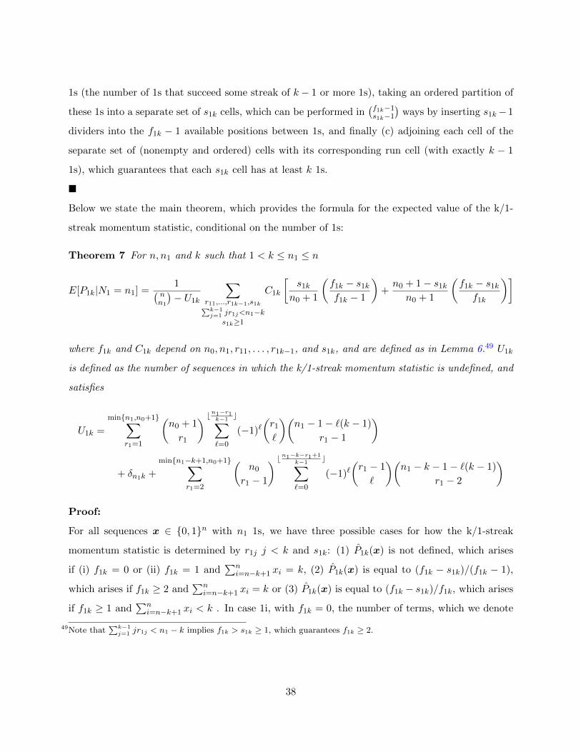
1s (the number of 1s that succeed some streak of k − 1 or more 1s), taking an ordered partition of

these 1s into a separate set of s1k cells, which can be performed in(f1k−1s1k−1

)ways by inserting s1k−1

dividers into the f1k − 1 available positions between 1s, and finally (c) adjoining each cell of the

separate set of (nonempty and ordered) cells with its corresponding run cell (with exactly k − 1

1s), which guarantees that each s1k cell has at least k 1s.

�

Below we state the main theorem, which provides the formula for the expected value of the k/1-

streak momentum statistic, conditional on the number of 1s:

Theorem 7 For n, n1 and k such that 1 < k ≤ n1 ≤ n

E[P1k|N1 = n1] =1(

nn1

)− U1k

∑r11,...,r1k−1,s1k∑k−1j=1 jr1j<n1−k

s1k≥1

C1k

[s1k

n0 + 1

(f1k − s1k

f1k − 1

)+n0 + 1− s1k

n0 + 1

(f1k − s1k

f1k

)]

where f1k and C1k depend on n0, n1, r11, . . . , r1k−1, and s1k, and are defined as in Lemma 6.49 U1k

is defined as the number of sequences in which the k/1-streak momentum statistic is undefined, and

satisfies

U1k =

min{n1,n0+1}∑r1=1

(n0 + 1

r1

) bn1−r1k−1c∑

`=0

(−1)`(r1

`

)(n1 − 1− `(k − 1)

r1 − 1

)

+ δn1k +

min{n1−k+1,n0+1}∑r1=2

(n0

r1 − 1

) bn1−k−r1+1k−1

c∑`=0

(−1)`(r1 − 1

`

)(n1 − k − 1− `(k − 1)

r1 − 2

)

Proof:

For all sequences x ∈ {0, 1}n with n1 1s, we have three possible cases for how the k/1-streak

momentum statistic is determined by r1j j < k and s1k: (1) P1k(x) is not defined, which arises

if (i) f1k = 0 or (ii) f1k = 1 and∑n

i=n−k+1 xi = k, (2) P1k(x) is equal to (f1k − s1k)/(f1k − 1),

which arises if f1k ≥ 2 and∑n

i=n−k+1 xi = k or (3) P1k(x) is equal to (f1k − s1k)/f1k, which arises

if f1k ≥ 1 and∑n

i=n−k+1 xi < k . In case 1i, with f1k = 0, the number of terms, which we denote

49Note that∑k−1j=1 jr1j < n1 − k implies f1k > s1k ≥ 1, which guarantees f1k ≥ 2.

38

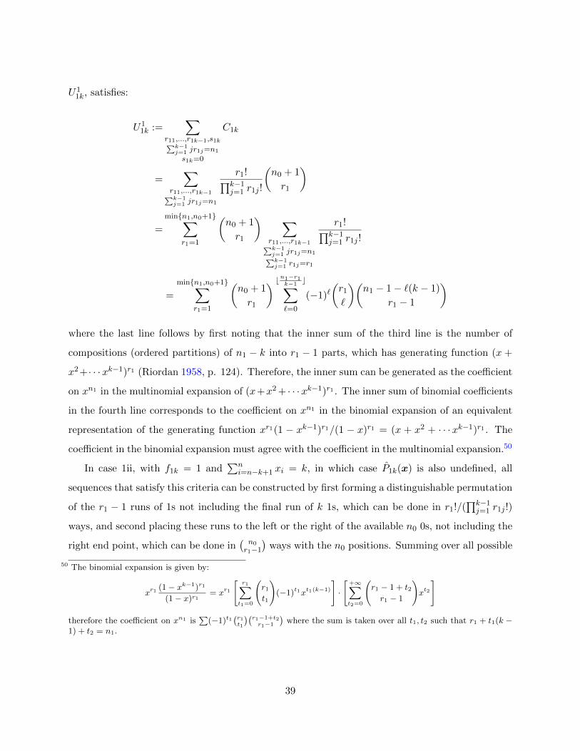
U11k, satisfies:

U11k :=

∑r11,...,r1k−1,s1k∑k−1

j=1 jr1j=n1

s1k=0

C1k

=∑

r11,...,r1k−1∑k−1j=1 jr1j=n1

r1!∏k−1j=1 r1j !

(n0 + 1

r1

)

=

min{n1,n0+1}∑r1=1

(n0 + 1

r1

) ∑r11,...,r1k−1∑k−1j=1 jr1j=n1∑k−1j=1 r1j=r1

r1!∏k−1j=1 r1j !

=

min{n1,n0+1}∑r1=1

(n0 + 1

r1

) bn1−r1k−1c∑

`=0

(−1)`(r1

`

)(n1 − 1− `(k − 1)

r1 − 1

)

where the last line follows by first noting that the inner sum of the third line is the number of

compositions (ordered partitions) of n1 − k into r1 − 1 parts, which has generating function (x +

x2+· · ·xk−1)r1 (Riordan 1958, p. 124). Therefore, the inner sum can be generated as the coefficient

on xn1 in the multinomial expansion of (x+x2 + · · ·xk−1)r1 . The inner sum of binomial coefficients

in the fourth line corresponds to the coefficient on xn1 in the binomial expansion of an equivalent

representation of the generating function xr1(1 − xk−1)r1/(1 − x)r1 = (x + x2 + · · ·xk−1)r1 . The

coefficient in the binomial expansion must agree with the coefficient in the multinomial expansion.50

In case 1ii, with f1k = 1 and∑n

i=n−k+1 xi = k, in which case P1k(x) is also undefined, all

sequences that satisfy this criteria can be constructed by first forming a distinguishable permutation

of the r1 − 1 runs of 1s not including the final run of k 1s, which can be done in r1!/(∏k−1j=1 r1j !)

ways, and second placing these runs to the left or the right of the available n0 0s, not including the

right end point, which can be done in(n0

r1−1

)ways with the n0 positions. Summing over all possible

50 The binomial expansion is given by:

xr1(1− xk−1)r1

(1− x)r1= xr1

[r1∑t1=0

(r1t1

)(−1)t1xt1(k−1)

]·

[+∞∑t2=0

(r1 − 1 + t2r1 − 1

)xt2

]

therefore the coefficient on xn1 is∑

(−1)t1(r1t1

)(r1−1+t2r1−1

)where the sum is taken over all t1, t2 such that r1 + t1(k −

1) + t2 = n1.

39

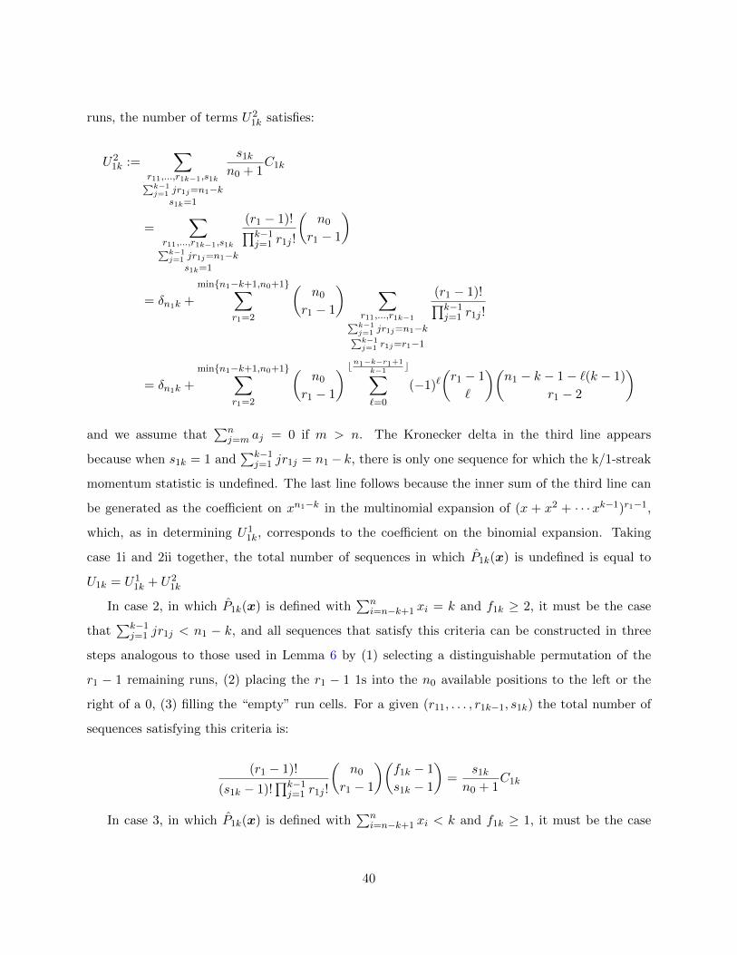
runs, the number of terms U21k satisfies:

U21k :=

∑r11,...,r1k−1,s1k∑k−1j=1 jr1j=n1−k

s1k=1

s1k

n0 + 1C1k

=∑

r11,...,r1k−1,s1k∑k−1j=1 jr1j=n1−k

s1k=1

(r1 − 1)!∏k−1j=1 r1j !

(n0

r1 − 1

)

= δn1k +

min{n1−k+1,n0+1}∑r1=2

(n0

r1 − 1

) ∑r11,...,r1k−1∑k−1j=1 jr1j=n1−k∑k−1j=1 r1j=r1−1

(r1 − 1)!∏k−1j=1 r1j !

= δn1k +

min{n1−k+1,n0+1}∑r1=2

(n0

r1 − 1

) bn1−k−r1+1k−1

c∑`=0

(−1)`(r1 − 1

`

)(n1 − k − 1− `(k − 1)

r1 − 2

)

and we assume that∑n

j=m aj = 0 if m > n. The Kronecker delta in the third line appears

because when s1k = 1 and∑k−1

j=1 jr1j = n1− k, there is only one sequence for which the k/1-streak

momentum statistic is undefined. The last line follows because the inner sum of the third line can

be generated as the coefficient on xn1−k in the multinomial expansion of (x + x2 + · · ·xk−1)r1−1,

which, as in determining U11k, corresponds to the coefficient on the binomial expansion. Taking

case 1i and 2ii together, the total number of sequences in which P1k(x) is undefined is equal to

U1k = U11k + U2

1k

In case 2, in which P1k(x) is defined with∑n

i=n−k+1 xi = k and f1k ≥ 2, it must be the case

that∑k−1

j=1 jr1j < n1 − k, and all sequences that satisfy this criteria can be constructed in three

steps analogous to those used in Lemma 6 by (1) selecting a distinguishable permutation of the

r1 − 1 remaining runs, (2) placing the r1 − 1 1s into the n0 available positions to the left or the

right of a 0, (3) filling the “empty” run cells. For a given (r11, . . . , r1k−1, s1k) the total number of

sequences satisfying this criteria is:

(r1 − 1)!

(s1k − 1)!∏k−1j=1 r1j !

(n0

r1 − 1

)(f1k − 1

s1k − 1

)=

s1k

n0 + 1C1k

In case 3, in which P1k(x) is defined with∑n

i=n−k+1 xi < k and f1k ≥ 1, it must be the case

40

that∑k−1

j=1 jr1j ≤ n1 − k, as before all sequences that satisfy this criteria can be constructed in

three steps as before, and we consider two subcases, sequences that terminate in a 1 (i.e. a run of

1s of length less than k) and sequences that terminate in a 0 (i.e. a run of 0s). For those sequence

that terminate in a 1, for a given (r11, . . . , r1k−1, s1k) the total number of sequences satisfying this

criteria is: (r1!

s1k!∏k−1j=1 r1j !

− (r1 − 1)!

(s1k − 1)!∏k−1j=1 r1j !

)(n0

r1 − 1

)(f1k − 1

s1k − 1

)=r1 − s1k

n0 + 1C1k

with (r1 − 1)!/((s1k − 1)!∏k−1j=1 r1j !) being the number of sequences that terminate in a run of 1s

of length k or more. For those sequences that terminate in a 0, for a given (r11, . . . , r1k−1, s1k) the

total number of sequences satisfying this criteria is:

r1!

s1k!∏k−1j=1 r1j !

(n0

r1

)(f1k − 1

s1k − 1

)=n0 + 1− r1

n0 + 1C1k

therefore, the sum of the k/1-streak momentum statistic across all sequences for which it is defined

satisfies:

E[P1k|N1 = n1]

[(n

n1

)− U1k

]=

∑r11,...,r1k−1,s1k∑k−1j=1 jr1j<n1−k

s1k≥1

C1ks1k

n0 + 1

f1k − s1k

f1k − 1

+∑

r11,...,r1k−1,s1k∑k−1j=1 jr1j≤n1−k

s1k≥1

C1kr1 − s1k

n0 + 1

f1k − s1k

f1k

+∑

r11,...,r1k−1,s1k∑k−1j=1 jr1j≤n1−k

s1k≥1

C1kn0 + 1− r1

n0 + 1

f1k − s1k

f1k

and this reduces to the formula in the theorem because the final two terms can be combined, and

then can be summed over only runs that satisfy∑k−1

j=1 jr1j < n1−k, and finally combined with the

first term (because f1k − s1k = 0 if∑k−1

j=1 jr1j = n1 − k).51

51While the first term has the closed form representation∑C1k

s1kn0+1

f1k−s1kf1k−1

=(n1−1k

)/(n−1k

), this does not appear to

be so for the other terms. E[P1k|N1 = n1] cannot have a closed form representation in any case, as the term U1k

does not allow one.

41

�

B.2 Expected Difference in Proportions

The exact formula for the expected difference between the relative frequency of 1 for k/1-streak

successor trials and the relative frequency of 1 for k/0-streak successor trials can be obtained with

an approach similar to that of the previous section. The difference satisfies Dk := P1k − (1− P0k),

and there are three categories of sequences for which Dk is defined: (1) a sequence that ends in

a run of 0s of length k or more, with f0k ≥ 2 and f1k ≥ 1, and the difference equal to D1k =

(f1k − s1k)/f1k − (s0k − 1)/(f0k − 1), (2) a sequence that ends in a run of 1s of length k or more,

with f0k ≥ 1 and f1k ≥ 2, and the difference equal to D2k := (f1k − s1k)/(f1k − 1) − s0k/f0k, (3)

a sequence that ends in a run of 0s of length k − 1, or less, or a run of 1s of length k − 1, or less,

with f0k ≥ 1 and f1k ≥ 1, and the difference equal to D3k := (f1k− s1k)/f1k− s0k/f0k. For all other

sequences the difference is undefined.

Theorem 8 For n, n1, n0 and k such that n0 + n1 = n, and 1 < k ≤ n0, n1 ≤ n, the expected

difference in the relative frequency of 1 for k/1-streak successors and the relative frequency of 1 for

42

k/0-streak successors, Dk := P1k − (1− P0k), satisfies

E[Dk | N1 = n1] =1(

nn1

)− Uk

∑

r01,...,r0k−1,s0kr11,...,r1k−1,s1k∑k−1

j=1 jr0j<n0−k,s0k≥1∑k−1j=1 jr1j≤n1−k,s1k≥1

r0≥r1

Ck

[s0k

r0D1k +

r0 − s0k

r0D3k

]

+∑

r01,...,r0k−1,s0kr11,...,r1k−1,s1k∑k−1

j=1 jr0j≤n0−k,s0k≥1∑k−1j=1 jr1j<n1−k,s1k≥1

r1≥r0

Ck

[s1k

r1D2k +

r1 − s1k

r1D3k

]

where D1k = (f1k − s1k)/f1k − (s0k − 1)/(f0k − 1), D2

k := (f1k − s1k)/(f1k − 1) − s0k/f0k, D3k :=

(f1k − s1k)/f1k − s0k/f0k, and

Ck :=r0!

s0k!∏k−1i=1 r0i!

r1!

s1k!∏k−1i=1 r1i!

(f0k − 1

s0k − 1

)(f1k − 1

s1k − 1

)

and Uk (see expression ∗ on page 47) is the number of sequences in which there are either no

k/1-streak successors, or no k/0-streak successors.

Proof:

Note that for the case in which |r1− r0| = 1, Ck is the number of sequences with N1 = n1 in which

the number of runs of 0s, and runs of 1s satisfy run profile (r01, . . . , r0k−1, s0k; r11, . . . , r1k−1, s1k);

for the cases in which r1 = r0, Ck is equal to half the number of these sequences (because each

sequence can end with a run of 1s, or a run of 0s). The combinatorial proof of this formula, which

we omit, is similar to the one used in the proof of Lemma 6.

43

The sum total of the differences, across all sequences for which the difference is defined and

N1 = n1 is

E[Dk | N1 = n1] ·[(

n

n1

)− Uk

]=

∑r01,...,r0k−1,s0kr11,...,r1k−1,s1k∑k−1

j=1 jr0j<n0−k,s0k≥1∑k−1j=1 jr1j≤n1−k,s1k≥1

r0≥r1

s0k

r0CkD

1k +

∑r01,...,r0k−1,s0kr11,...,r1k−1,s1k∑k−1

j=1 jr0j≤n0−k,s0k≥1∑k−1j=1 jr1j<n1−k,s1k≥1

r1≥r0

s1k

r1CkD

2k

+∑

r01,...,r0k−1,s0kr11,...,r1k−1,s1k∑k−1

j=1 jr0j≤n0−k,s0k≥1∑k−1j=1 jr1j≤n1−k,s1k≥1

r0≥r1

r0 − s0k

r0CkD

3k +

∑r01,...,r0k−1,s0kr11,...,r1k−1,s1k∑k−1

j=1 jr0j≤n0−k,s0k≥1∑k−1j=1 jr1j≤n1−k,s1k≥1

r1≥r0

r1 − s1k

r1CkD

3k

where the first sum relates to those sequences that end in a run of 0s of length k or more (whence

r0 ≥ r1, the multiplier s0k/r0 and∑k−1

j=1 jr0j < n0−k);52 the second sum relates to those sequences

that end in a run of 1s of length k or more (whence r1 ≥ r0, the multiplier s1k/r1 and∑k−1

j=1 jr1j <

n1−k); the third sum relates to those sequences that end on a run of 0s of length k-1 or less (whence

r0 ≥ r1, the multiplier (r0 − s0k)/r0) and∑k−1

j=1 jr0j < n0 − k);53 and the fourth sum relates to

those sequences that end on a run of 1s of length k − 1 or less (whence r1 ≥ r0, the multiplier

(r1 − s1k)/r1) and∑k−1

j=1 jr1j < n1 − k). These four terms can be combined into the following two

52Note∑k−1j=1 jr0j < n0 − k ⇐⇒ f0k ≥ 2.

53The multiplier (r0 − s0k)/r0 arises because the number of distinguishable permutations of the 0 runs that end witha run of length k − 1 or less is equal to the total number of distinguishable permutations of the 0 runs minus thenumber of distinguishable permutations of the 0 runs that end in a run of length k or more, i.e.

r0!

s0k!∏k−1i=1 r0i!

− (r0 − 1)!

(s0k − 1)!∏k−1i=1 r0i!

=r0 − s0kr0

r0!

s0k!∏k−1i=1 r0i!

44

terms:

E[Dk | N1 = n1] ·[(

n

n1

)− Uk

]=

∑r01,...,r0k−1,s0kr11,...,r1k−1,s1k∑k−1

j=1 jr0j<n0−k,s0k≥1∑k−1j=1 jr1j≤n1−k,s1k≥1

r0≥r1

Ck

[s0k

r0D1k +

r0 − s0k

r0D3k

]

+∑

r01,...,r0k−1,s0kr11,...,r1k−1,s1k∑k−1

j=1 jr0j≤n0−k,s0k≥1∑k−1j=1 jr1j<n1−k,s1k≥1

r1≥r0

Ck

[s1k

r1D2k +

r1 − s1k

r1D3k

]

which can readily be implemented numerically for the finite sequences considered here.54 The total

number of sequences for which the difference is undefined, Uk, can be counted in a way that is

analogous to what was done in the proof of Theorem 7, by using an application of the inclusion-

exclusion principle:

Uk :=∑

r11,...,r1k−1,s1k∑k−1j=1 jr1j=n1

s1k=0

C1k +∑

r11,...,r1k−1,s1k∑k−1j=1 jr1j=n1−k

s1k=1

s1k

n0 + 1C1k +

∑r01,...,r0k−1,s0k∑k−1

j=1 jr0j=n1

s0k=0

C0k +∑

r01,...,r0k−1,s0k∑k−1j=1 jr0j=n1−k

s0k=1

s0k

n1 + 1C0k

−∑

r01,...,r0k−1,s0kr11,...,r1k−1,s1k∑k−1j=1 jr0j=n0,s0k=0∑k−1j=1 jr1j=n1,s1k=0

|r0−r1|≤1

(2 · 1{r1=r0} + 1{|r1−r0|=1}

)Ck

−∑

r01,...,r0k−1,s0kr11,...,r1k−1,s1k∑k−1

j=1 jr0j=n0−k,s0k=1∑k−1j=1 jr1j=n1,s1k=0

r0≥r1

s0k

r0Ck −

∑r01,...,r0k−1,s0kr11,...,r1k−1,s1k∑k−1j=1 jr0j=n0,s0k=0∑k−1

j=1 jr1j=n1−k,s1k=1

r1≥r0

s1k

r1Ck

54In the numerical implementation one can consider three sums r0 = r1 + 1, r1 = r0 + 1, and for the case of r1 = r0the sums can be combined.

45

where C0k is a function of r01, . . . , r0k−1, s0k;n0, n1 and defined analogously to C1k. We can simplify

the above expression by first noting that the third term, which corresponds to those sequences in

which there are no k/1-streak successors and no k/0-streak successors, can be reduced to a sum of

binomial coefficients:

∑r01,...,r0k−1,s0kr11,...,r1k−1,s1k∑k−1j=1 jr0j=n0,s0k=0∑k−1j=1 jr1j=n1,s1k=0

|r0−r1|≤1

(2 · 1{r1=r0} + 1{|r1−r0|=1}

)Ck

=∑

r01,...,r0k−1,s0kr11,...,r1k−1,s1k∑k−1j=1 jr0j=n0,s0k=0∑k−1j=1 jr1j=n1,s1k=0

|r0−r1|≤1

(2 · 1{r1=r0} + 1{|r1−r0|=1}

) r0!

s0k!∏k−1i=1 r0i!

r1!

s1k!∏k−1i=1 r1i!

=∑

r01,...,r0k−1r11,...,r1k−1∑k−1j=1 jr0j=n0∑k−1j=1 jr1j=n1

|r0−r1|≤1

(2 · 1{r1=r0} + 1{|r1−r0|=1}

) r0!∏k−1i=1 r0i!

r1!∏k−1i=1 r1i!

=

min{n1,n0+1}∑r1=1

min{r1+1,n0}∑r0=max{r1−1,1}

(2 · 1{r1=r0} + 1{|r1−r0|=1}

) ∑r01,...,r0k−1r11,...,r1k−1∑k−1j=1 jr0j=n0∑k−1j=1 jr1j=n1∑k−1j=1 r0j=r0∑k−1j=1 r1j=r1

r0!∏k−1i=1 r0i!

r1!∏k−1i=1 r1i!

=

min{n1,n0+1}∑r1=1

min{r1+1,n0}∑r0=max{r1−1,1}

(2 · 1{r1=r0} + 1{|r1−r0|=1}

) ∑r01,...,r0k−1∑k−1j=1 jr0j=n0∑k−1j=1 r0j=r0

r0!∏k−1i=1 r0i!

∑r11,...,r1k−1∑k−1j=1 jr1j=n1∑k−1j=1 r1j=r1

r1!∏k−1i=1 r1i!

=

min{n1,n0+1}∑r1=1

min{r1+1,n0}∑r0=max{r1−1,1}

(2 · 1{r1=r0} + 1{|r1−r0|=1}

) bn0−r0k−1c∑

`0=0

(−1)`0(r0

`0

)(n0 − 1− `0(k − 1)

r0 − 1

)

×bn1−r1k−1

c∑`1=0

(−1)`1(r1

`1

)(n1 − 1− `1(k − 1)

r1 − 1

)

46

For the final two negative terms in the formula for Uk, we can apply a similar argument in order to

represent them as a sum of binomial coefficients. For the first four positive terms we can use the

argument provided in Theorem 7 to represent them as sums of binomial coefficients, and therefore

Uk reduces to a sum of binomial coefficients:

Uk =

min{n1,n0+1}∑r1=1

(n0 + 1

r1

) bn1−r1k−1c∑

`=0

(−1)`(r1

`

)(n1 − 1− `(k − 1)

r1 − 1

)(*)

+ δn1k +

min{n1−k+1,n0+1}∑r1=2

(n0

r1 − 1

) bn1−k−r1+1k−1

c∑`=0

(−1)`(r1 − 1

`

)(n1 − k − 1− `(k − 1)

r1 − 2

)

+

min{n0,n1+1}∑r0=1

(n1 + 1

r0

) bn0−r0k−1c∑

`=0

(−1)`(r0

`

)(n0 − 1− `(k − 1)

r0 − 1

)

+ δn0k +

min{n0−k+1,n1+1}∑r0=2

(n1

r0 − 1

) bn0−k−r0+1k−1

c∑`=0

(−1)`(r0 − 1

`

)(n0 − k − 1− `(k − 1)

r0 − 2

)

−

min{n1,n0+1}∑r1=1

min{r1+1,n0}∑r0=max{r1−1,1}

(2 · 1{r1=r0} + 1{|r1−r0|=1}

)×

×bn0−r0k−1

c∑`0=0

(−1)`0(r0

`0

)(n0 − 1− `0(k − 1)

r0 − 1

) bn1−r1k−1c∑

`1=0

(−1)`1(r1

`1

)(n1 − 1− `1(k − 1)

r1 − 1

)−

δn0k +

min{n0−k+1,n1+1}∑r0=2

min{r0,n1}∑r1=max{r0−1,1}

bn0−k−r0+1k−1

c∑`0=0

(−1)`0(r0 − 1

`0

)(n0 − k − 1− `0(k − 1)

r0 − 2

)×

×bn1−r1k−1

c∑`1=0

(−1)`1(r1

`1

)(n1 − 1− `1(k − 1)

r1 − 1

)−

δn1k +

min{n1−k+1,n0+1}∑r1=2

min{r1,n0}∑r0=max{r1−1,1}

bn1−k−r1+1k−1

c∑`1=0

(−1)`1(r1 − 1

`1

)(n1 − k − 1− `1(k − 1)

r1 − 2

)×

×bn0−r0k−1

c∑`0=0

(−1)`0(r0

`0

)(n0 − 1− `0(k − 1)

r0 − 1

)

47

�

C Appendix: Why it often is the case that E[P1k|N1 = n1] <n1−kn−k .

For an intuition why the sampling without replacement reasoning that worked when k = 1 does

not extend to k > 1, we first note that E[P1k|N1 = n1] is given by:

E[P1k(x)|N1(x) = n1] = E

[ ∑n1j=k(j − k)R1j(x)∑n1

j=k(j − k + 1)R1j(x)−∏ni=n−k+1 xi

∣∣∣∣∣N1(x) = n1

](†)

(as in Appendix B), where, for simplicity, we assume that n1 > (k − 1)n0 + k (to avoid the

possibility of missing observations). This formula can be operationalized as the probability of

observing a 1 in the following two-step procedure, which we call “Procedure A”: (1) selecting, at

random, one of the equiprobable(nn1

)sequences, and (2) from that sequence, selecting, at random,

one of the trials that immediately follows a streak of k or more 1s (this procedure is analogous to

that discussed in the alternate proof of Lemma 3). We now explain why the probability generated

by this procedure is typically strictly less than n1−kn−k . First, imagine (counterfactually) that for each

sequence x = (x1, . . . , xn) that satisfies N1(x) = n1, we have R1i(x) = E[R1i(x)|N1(x) = n1] for

i = 1, . . . n1, i.e. the joint profile of run lengths is constant across sequences, and the number of runs

of each length is equal to its expected value, conditional on n1 successes (assuming divisibility).

Further, assume that∏ni=n−k+1 xi = E[

∏ni=n−k+1 xi|N1(x) = n1], i.e. replace, with its expected

value, the variable that equals one when a single trial must be removed from the denominator

(because the sequence ends in a run of 1s of length j ≥ k, leaving the final trial in the run without

a successor). In this counterfactual case, we will see below that † can now be operationalized as the

probability of observing a 1 in the simpler “Procedure B”: selecting a trial at random (uniformly)

from the pooled set of trials that (a) appear in one of the(nn1

)sequences with n1 successes and (b)

immediately follow k or more 1s. To see this, first note that because each sequence has the same

joint profile of run lengths, the right hand side in the equation † becomes the left hand side in the

48

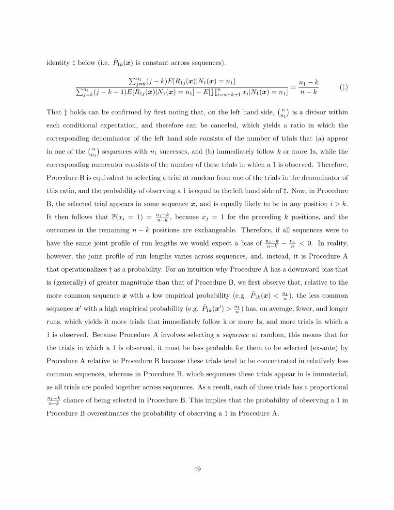
identity ‡ below (i.e. P1k(x) is constant across sequences).

∑n1j=k(j − k)E[R1j(x)|N1(x) = n1]∑n1

j=k(j − k + 1)E[R1j(x)|N1(x) = n1]− E[∏ni=n−k+1 xi|N1(x) = n1]

=n1 − kn− k

(‡)

That ‡ holds can be confirmed by first noting that, on the left hand side,(nn1

)is a divisor within

each conditional expectation, and therefore can be canceled, which yields a ratio in which the

corresponding denominator of the left hand side consists of the number of trials that (a) appear

in one of the(nn1

)sequences with n1 successes, and (b) immediately follow k or more 1s, while the

corresponding numerator consists of the number of these trials in which a 1 is observed. Therefore,

Procedure B is equivalent to selecting a trial at random from one of the trials in the denominator of

this ratio, and the probability of observing a 1 is equal to the left hand side of ‡. Now, in Procedure

B, the selected trial appears in some sequence x, and is equally likely to be in any position i > k.

It then follows that P(xi = 1) = n1−kn−k , because xj = 1 for the preceding k positions, and the

outcomes in the remaining n − k positions are exchangeable. Therefore, if all sequences were to

have the same joint profile of run lengths we would expect a bias of n1−kn−k −

n1n < 0. In reality,

however, the joint profile of run lengths varies across sequences, and, instead, it is Procedure A

that operationalizes † as a probability. For an intuition why Procedure A has a downward bias that

is (generally) of greater magnitude than that of Procedure B, we first observe that, relative to the

more common sequence x with a low empirical probability (e.g. P1k(x) < n1n ), the less common

sequence x′ with a high empirical probability (e.g. P1k(x′) > n1

n ) has, on average, fewer, and longer

runs, which yields it more trials that immediately follow k or more 1s, and more trials in which a

1 is observed. Because Procedure A involves selecting a sequence at random, this means that for

the trials in which a 1 is observed, it must be less probable for them to be selected (ex-ante) by

Procedure A relative to Procedure B because these trials tend to be concentrated in relatively less

common sequences, whereas in Procedure B, which sequences these trials appear in is immaterial,

as all trials are pooled together across sequences. As a result, each of these trials has a proportional

n1−kn−k chance of being selected in Procedure B. This implies that the probability of observing a 1 in

Procedure B overestimates the probability of observing a 1 in Procedure A.

49

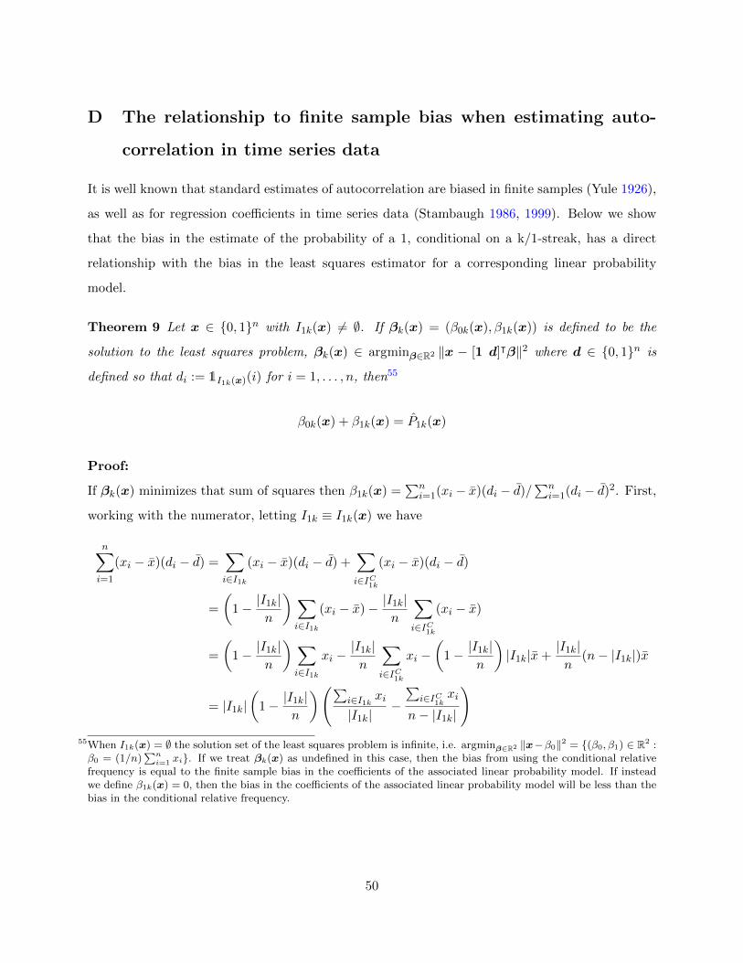
D The relationship to finite sample bias when estimating auto-

correlation in time series data

It is well known that standard estimates of autocorrelation are biased in finite samples (Yule 1926),

as well as for regression coefficients in time series data (Stambaugh 1986, 1999). Below we show

that the bias in the estimate of the probability of a 1, conditional on a k/1-streak, has a direct

relationship with the bias in the least squares estimator for a corresponding linear probability

model.

Theorem 9 Let x ∈ {0, 1}n with I1k(x) 6= ∅. If βk(x) = (β0k(x), β1k(x)) is defined to be the

solution to the least squares problem, βk(x) ∈ argminβ∈R2 ‖x − [1 d]ᵀβ‖2 where d ∈ {0, 1}n is

defined so that di := 1I1k(x)(i) for i = 1, . . . , n, then55

β0k(x) + β1k(x) = P1k(x)

Proof:

If βk(x) minimizes that sum of squares then β1k(x) =∑n

i=1(xi − x)(di − d)/∑n

i=1(di − d)2. First,

working with the numerator, letting I1k ≡ I1k(x) we have

n∑i=1

(xi − x)(di − d) =∑i∈I1k

(xi − x)(di − d) +∑i∈IC1k

(xi − x)(di − d)

=

(1− |I1k|

n

) ∑i∈I1k

(xi − x)− |I1k|n

∑i∈IC1k

(xi − x)

=

(1− |I1k|

n

) ∑i∈I1k

xi −|I1k|n

∑i∈IC1k

xi −(

1− |I1k|n

)|I1k|x+

|I1k|n

(n− |I1k|)x

= |I1k|(

1− |I1k|n

)(∑i∈I1k xi

|I1k|−∑

i∈IC1kxi

n− |I1k|

)55When I1k(x) = ∅ the solution set of the least squares problem is infinite, i.e. argminβ∈R2 ‖x−β0‖2 = {(β0, β1) ∈ R2 :β0 = (1/n)

∑ni=1 xi}. If we treat βk(x) as undefined in this case, then the bias from using the conditional relative

frequency is equal to the finite sample bias in the coefficients of the associated linear probability model. If insteadwe define β1k(x) = 0, then the bias in the coefficients of the associated linear probability model will be less than thebias in the conditional relative frequency.

50

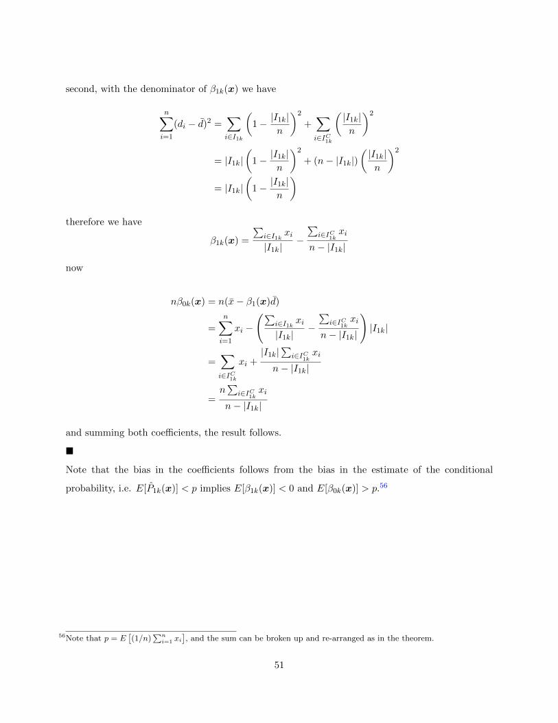
second, with the denominator of β1k(x) we have

n∑i=1

(di − d)2 =∑i∈I1k

(1− |I1k|

n

)2

+∑i∈IC1k

(|I1k|n

)2

= |I1k|(

1− |I1k|n

)2

+ (n− |I1k|)(|I1k|n

)2

= |I1k|(

1− |I1k|n

)

therefore we have

β1k(x) =

∑i∈I1k xi

|I1k|−∑

i∈IC1kxi

n− |I1k|

now

nβ0k(x) = n(x− β1(x)d)

=n∑i=1

xi −

(∑i∈I1k xi

|I1k|−∑

i∈IC1kxi

n− |I1k|

)|I1k|

=∑i∈IC1k

xi +|I1k|

∑i∈IC1k

xi

n− |I1k|

=n∑

i∈IC1kxi

n− |I1k|

and summing both coefficients, the result follows.

�

Note that the bias in the coefficients follows from the bias in the estimate of the conditional

probability, i.e. E[P1k(x)] < p implies E[β1k(x)] < 0 and E[β0k(x)] > p.56

56Note that p = E[(1/n)

∑ni=1 xi

], and the sum can be broken up and re-arranged as in the theorem.

51