Embed Size (px)
Citation preview
Review of Economic Studies (2010) 77, 730–778 0034-6527/10/00411011$02.00© 2009 The Review of Economic Studies Limited doi: 10.1111/j.1467-937X.2009.00582.x
The Gambler’s and Hot-HandFallacies: Theory and
ApplicationsMATTHEW RABIN
University of California, Berkeley
and
DIMITRI VAYANOSLondon School of Economics, CEPR and NBER
First version received September 2007; final version accepted May 2009 (Eds.)
We develop a model of the gambler’s fallacy—the mistaken belief that random sequences shouldexhibit systematic reversals. We show that an individual who holds this belief and observes a sequenceof signals can exaggerate the magnitude of changes in an underlying state but underestimate theirduration. When the state is constant, and so signals are i.i.d., the individual can predict that longstreaks of similar signals will continue—a hot-hand fallacy. When signals are serially correlated, theindividual typically under-reacts to short streaks, over-reacts to longer ones, and under-reacts to verylong ones. Our model has implications for a number of puzzles in finance, e.g. the active-fund andfund-flow puzzles, and the presence of momentum and reversal in asset returns.
1. INTRODUCTION
Many people fall under the spell of the “gambler’s fallacy”, expecting outcomes in randomsequences to exhibit systematic reversals. When observing flips of a fair coin, for example,people believe that a streak of heads makes it more likely that the next flip will be a tail. Thegambler’s fallacy is commonly interpreted as deriving from a fallacious belief in the “law ofsmall numbers” or “local representativeness”: people believe that a small sample should resem-ble closely the underlying population, and hence believe that heads and tails should balanceeven in small samples. On the other hand, people also sometimes predict that random sequenceswill exhibit excessive persistence rather than reversals. While basketball fans believe that play-ers have “hot hands”, being more likely than average to make the next shot when currently ona hot streak, several studies have shown that no perceptible streaks justify such beliefs.1
At first blush, the hot-hand fallacy appears to directly contradict the gambler’s fallacybecause it involves belief in excessive persistence rather than reversals. Several researchers
1. The representativeness bias is perhaps the most commonly explored bias in judgement research. Section 2reviews evidence on the gambler’s fallacy, and a more extensive review can be found in Rabin (2002). For evidenceon the hot-hand fallacy, see, for example, Gilovich, Vallone and Tversky (1985) and Tversky and Gilovich (1989a,b).See also Camerer (1989) who shows that betting markets for basketball games exhibit a small hot-hand bias.
730
RABIN & VAYANOS THE GAMBLER’S AND HOT-HAND FALLACIES 731
have, however, suggested that the two fallacies might be related, with the hot-hand fallacyarising as a consequence of the gambler’s fallacy.2 Suppose that an investor prone to the gam-bler’s fallacy observes the performance of a mutual fund, which can depend on the manager’sability and luck. Convinced that luck should reverse, the investor underestimates the likelihoodthat a manager of average ability will exhibit a streak of above- or below-average performances.Following good or bad streaks, therefore, the investor over-infers that the current manager isabove or below average, and so in turn predicts continuation of unusual performances.
This paper develops a model to examine the link between the gambler’s fallacy and thehot-hand fallacy, as well as the broader implications of the fallacies for people’s predictions andactions in economic and financial settings. In our model, an individual observes a sequenceof signals that depend on an unobservable underlying state. We show that because of thegambler’s fallacy, the individual is prone to exaggerate the magnitude of changes in the state,but underestimate their duration. We characterize the individual’s predictions following streaksof similar signals, and determine when a hot-hand fallacy can arise. Our model has implicationsfor a number of puzzles in finance, e.g. the active-fund and fund-flow puzzles, and the presenceof momentum and reversal in asset returns.
While providing extensive motivation and elaboration in Section 2, we now present themodel itself in full. An agent observes a sequence of signals whose probability distributiondepends on an underlying state. The signal st in period t = 1, 2, . . . is
st = θ t + εt , (1)
where θ t is the state and εt an i.i.d. normal shock with mean zero and variance σ 2ε > 0. The
state evolves according to the auto-regressive process
θ t = ρθt−1 + (1 − ρ)(μ + ηt ), (2)
where ρ ∈ [0, 1] is the persistence parameter, μ the long-run mean, and ηt an i.i.d. normalshock with mean zero, variance σ 2
η, and independent of εt . As an example that we shall returnto often, consider a mutual fund run by a team of managers. We interpret the signal as thefund’s return, the state as the managers’ average ability, and the shock εt as the managers’luck. Assuming that the ability of any given manager is constant over time, we interpret 1 − ρ
as the rate of managerial turnover, and σ 2η as the dispersion in ability across managers.3
We model the gambler’s fallacy as the mistaken belief that the sequence {εt }t≥1 is not i.i.d.,but rather exhibits reversals: according to the agent,
εt = ωt − αρ
∞∑k=0
δkρεt−1−k, (3)
where the sequence {ωt }t≥1 is i.i.d. normal with mean zero and variance σ 2ω, and (αρ, δρ) are
parameters in [0, 1) that can depend on ρ.4 Consistent with the gambler’s fallacy, the agent
2. See, for example, Camerer (1989) and Rabin (2002). The causal link between the gambler’s fallacy andthe hot-hand fallacy is a common intuition in psychology. Some suggestive evidence comes from an experiment byEdwards (1961), in which subjects observe a very long binary series and are given no information about the generatingprocess. Subjects seem, by the evolution of their predictions over time, to come to believe in a hot hand. Since theactual generating process is independent and identically distributed (i.i.d.), this is suggestive that a source of the hothand is the perception of too many long streaks.
3. Alternatively, we can assume that a fraction 1 − ρ of existing managers get a new ability “draw” in anygiven period. Ability could be time-varying if, for example, managers’ expertise is best suited to specific marketconditions. We use the managerial-turnover interpretation because it is easier for exposition.
4. We set εt = 0 for t ≤ 0, so that all terms in the infinite sum are well defined.
© 2009 The Review of Economic Studies Limited
732 REVIEW OF ECONOMIC STUDIES
believes that high realizations of εt ′ in period t ′ < t make a low realization more likely inperiod t . The parameter αρ measures the strength of the effect, while δρ measures the relativeinfluence of realizations in the recent and more distant past. We mainly focus on the case where(αρ, δρ) depend linearly on ρ, i.e. (αρ, δρ) = (αρ, δρ) for α, δ ∈ [0, 1). Section 2 motivateslinearity based on the assumption that people expect reversals only when all outcomes in arandom sequence are drawn from the same distribution, e.g. the performances of a fund managerwhose ability is constant over time. This assumption rules out belief in mean reversion acrossdistributions; e.g. a good performance by one manager does not make another manager duefor a bad performance next period. If managers turn over frequently (ρ is small) therefore, thegambler’s fallacy has a small effect, consistent with the linear specification. Section 2 discussesalternative specifications for (αρ, δρ) and the link with the evidence. Appendix A shows thatthe agent’s error patterns in predicting the signals are very similar across specifications.
Section 3 examines how the agent uses the sequence of past signals to make inferencesabout the underlying parameters and to predict future signals. We assume that the agent infersas a fully rational Bayesian and fully understands the structure of his environment, except fora mistaken and dogmatic belief that α > 0. From observing the signals, the agent learns aboutthe underlying state θ t , and possibly about the parameters of his model (σ 2
η, ρ, σ 2ω, μ) if these
are unknown.5
In the benchmark case where the agent is certain about all model parameters, his inferencecan be treated using standard tools of recursive (Kalman) filtering, where the gambler’s fallacyessentially expands the state vector to include not only the state θ t but also a statistic of pastluck realizations. If instead the agent is uncertain about parameters, recursive filtering can beused to evaluate the likelihood of signals conditional on parameters. An appropriate version ofthe law of large numbers (LLN) implies that after observing many signals, the agent convergeswith probability 1 to parameter values that maximize a limit likelihood. While the likelihoodfor α = 0 is maximized for limit posteriors corresponding to the true parameter values, theagent’s abiding belief that α > 0 leads him generally to false limit posteriors. Identifying whenand how these limit beliefs are wrong is the crux of our analysis.6
Section 4 considers the case where signals are i.i.d. because σ 2η = 0.7 If the agent is initially
uncertain about parameters and does not rule out any possible value, then he converges to thebelief that ρ = 0. Under this belief, he predicts the signals correctly as i.i.d., despite thegambler’s fallacy. The intuition is that he views each signal as drawn from a new distribution;
5. When learning about model parameters, the agent is limited to models satisfying equations (1) and (2). Sincethe true model belongs to that set, considering models outside the set does not change the limit outcome of rationallearning. An agent prone to the gambler’s fallacy, however, might be able to predict the signals more accurately usingan incorrect model, as the two forms of error might offset each other. Characterizing the incorrect model that theagent converges to is central to our analysis, but we restrict such a model to satisfy equations (1) and (2). A modelnot satisfying equations (1) and (2) can help the agent make better predictions when signals are serially correlated.See footnote 24.
6. Our analysis has similarities to model mis-specification in econometrics. Consider, for example, the classicomitted-variables problem, where the true model is Y = α + β1X1 + β2X2 + ε but an econometrician estimatesY = α + β1X1 + ε. The omission of the variable X2 can be interpreted as a dogmatic belief that β2 = 0. When thisbelief is incorrect because β2 �= 0, the econometrician’s estimate of β1 is biased and inconsistent (e.g. Greene, 2008,Ch. 7). Mis-specification in econometric models typically arises because the true model is more complicated thanthe econometrician’s model. In our setting the agent’s model is the more complicated because it assumes negativecorrelation where there is none.
7. When σ 2η = 0, the shocks ηt are equal to zero, and therefore equation (2) implies that in steady state θ t is
constant.
© 2009 The Review of Economic Studies Limited
RABIN & VAYANOS THE GAMBLER’S AND HOT-HAND FALLACIES 733
e.g. new managers run the fund in each period. Therefore, his belief that any given manager’sperformance exhibits mean reversion has no effect.
We next assume that the agent knows on prior grounds that ρ > 0; e.g. is aware that man-agers stay in the fund for more than one period. Ironically, the agent’s correct belief ρ > 0can lead him astray. This is because he cannot converge to the belief ρ = 0, which, whileincorrect, enables him to predict the signals correctly. Instead, he converges to the smallestvalue of ρ to which he gives positive probability. He also converges to a positive value ofσ 2
η, believing falsely that managers differ in ability, so that (given turnover) there is variationover time in average ability. This belief helps him to explain the incidence of streaks despitethe gambler’s fallacy: a streak of high returns, for example, can be readily explained throughthe belief that good managers might have joined the fund recently. Of course, the agent thinksthat the streak might also have been due to luck, and expects a reversal. We show that theexpectation of a reversal dominates for short streaks, but because reversals that do not happenmake the agent more confident the managers have changed, he expects long streaks to continue.Thus, predictions following long streaks exhibit a hot-hand fallacy.8
Section 5 relaxes the assumption that σ 2η = 0, to consider the case where signals are seri-
ally correlated. As in the i.i.d. case, the agent underestimates ρ and overestimates the variance(1 − ρ)2σ 2
η of the shocks to the state. He does not converge, however, all the way to ρ = 0because he must account for the signals’ serial correlation. Because he views shocks to thestate as overly large in magnitude, he treats signals as very informative, and tends to over-react to streaks. For very long streaks, however, there is under-reaction because the agent’sunderestimation of ρ means that he views the information learned from the signals as overlyshort-lived. Under-reaction also tends to occur following short streaks because of the basicgambler’s fallacy intuition.
In summary, Sections 4 and 5 confirm the oft-conjectured link from the gambler’s to thehot-hand fallacy, and generate novel predictions which can be tested in experimental or fieldsettings. We summarize the predictions at the end of Section 5.
We conclude this paper in Section 6 by exploring finance applications. One applicationconcerns the belief in financial expertise. Suppose that returns on traded assets are i.i.d., andwhile the agent does not rule out that expected returns are constant, he is confident that anyshocks to expected returns should last for more than one period (ρ > 0). He then ends upbelieving that returns are predictable on the basis of past history, and exaggerates the valueof financial experts if he believes that the experts’ advantage derives from observing marketinformation. This could help explain the active-fund puzzle, namely why people invest inactively managed funds in spite of the evidence that these funds underperform their passivelymanaged counterparts. In a related application we show that the agent not only exaggerates thevalue added by active managers but also believes that this value varies over time. This couldhelp explain the fund-flow puzzle, namely that flows into mutual funds are positively correlatedwith the funds’ lagged returns, and yet lagged returns do not appear to predict future returns.Our model could also speak to other finance puzzles, such as the presence of momentum andreversals in asset returns and the value premium.
Our work is related to Rabin’s (2002) model of the law of small numbers. In Rabin, anagent draws balls from an urn with replacement but believes that replacement occurs only everyodd period. Thus, the agent overestimates the probability that the ball drawn in an even period
8. We are implicitly defining the hot-hand fallacy as a belief in the continuation of streaks. An alternativeand closely related definition involves the agent’s assessed auto-correlation of the signals. See footnote 22 and thepreceding text.
© 2009 The Review of Economic Studies Limited
734 REVIEW OF ECONOMIC STUDIES
is of a different colour than the one drawn in the previous period. Because of replacement,the composition of the urn remains constant over time. Thus, the underlying state is constant,which corresponds to ρ = 1 in our model. We instead allow ρ to take any value in [0, 1)
and show that the agent’s inferences about ρ significantly affect his predictions of the signals.Additionally, because ρ < 1, we can study inference in a stochastic steady state and conduct atrue dynamic analysis of the hot-hand fallacy (showing how the effects of good and bad streaksalternate over time). Because of the steady state and the normal-linear structure, our modelis more tractable than Rabin’s. In particular, we characterize fully predictions after streaksof signals, while Rabin can do so only with numerical examples and for short streaks. Thefinance applications in Section 6 illustrate further our model’s tractability and applicability,while also leading to novel insights such as the link between the gambler’s fallacy and beliefin outperformance of active funds.
Our work is also related to the theory of momentum and reversals of Barberis, Shleifer andVishny (1998). In BSV, investors do not realize that innovations to a company’s earnings arei.i.d. Rather, they believe them to be drawn either from a regime with excess reversals or fromone with excess streaks. If the reversal regime is the more common, the stock price under-reacts to short streaks because investors expect a reversal. The price over-reacts, however, tolonger streaks because investors interpret them as sign of a switch to the streak regime. Thiscan generate short-run momentum and long-run reversals in stock returns, consistent with theempirical evidence, surveyed in BSV. It can also generate a value premium because stockswith long positive (negative) streaks become overvalued (undervalued) relative to earningsand yield low (high) expected returns. Our model has similar implications because in i.i.d.settings the agent can expect short streaks to reverse and long streaks to continue. But whilethe implications are similar, our approach is different. BSV provide a psychological foundationfor their assumptions by appealing to a combination of biases: the conservatism bias for thereversal regime and the representativeness bias for the streak regime. Our model, by contrast,not only derives such biases from the single underlying bias of the gambler’s fallacy, but indoing so provides predictions as to which biases are likely to appear in different informationalsettings.9
2. MOTIVATION FOR THE MODEL
Our model is fully described by equations (1) to (3) presented in the Introduction. In thissection, we motivate the model by drawing the connection with the experimental evidence onthe gambler’s fallacy. A difficulty with using this evidence is that most experiments concernsequences that are binary and i.i.d., such as coin flips. Our goal, by contrast, is to explorethe implications of the gambler’s fallacy in richer settings. In particular, we need to considernon-i.i.d. settings since the hot-hand fallacy involves a belief that the world is non-i.i.d. Theexperimental evidence gives little direct guidance on how the gambler’s fallacy would mani-fest itself in non-binary, non-i.i.d. settings. In this section, however, we argue that our modelrepresents a natural extrapolation of the gambler’s fallacy “logic” to such settings. Of course,any such extrapolation has an element of speculativeness. But, if nothing else, our specificationof the gambler’s fallacy in the new settings can be viewed as a working hypothesis about the
9. Even in settings where error patterns in our model resemble those in BSV, there are important differences.For example, the agent’s expectation of a reversal can increase with streak length for short streaks, while in BSV itunambiguously decreases (as it does in Rabin (2002) because the expectation of a reversal lasts for only one period).This increasing pattern is a key finding of an experimental study by Asparouhova, Hertzel and Lemmon (2008). Seealso Bloomfield and Hales (2002).
© 2009 The Review of Economic Studies Limited
RABIN & VAYANOS THE GAMBLER’S AND HOT-HAND FALLACIES 735
broader empirical nature of the phenomenon that both highlights features of the phenomenonthat seem to matter and generates testable predictions for experimental and field research.
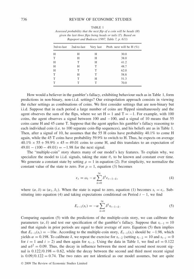
Experiments documenting the gambler’s fallacy are mainly of three types: production tasks,where subjects are asked to produce sequences that look to them like random sequences of coinflips; recognition tasks, where subjects are asked to identify which sequences look like coinflips; and prediction tasks, where subjects are asked to predict the next outcome in coin-flipsequences. In all types of experiments, the typical subject identifies a switching (i.e. reversal)rate greater than 50% to be indicative of random coin flips.10 The most carefully reported datafor our purposes comes from the production-task study of Rapoport and Budescu (1997). Usingtheir Table 7, we estimate in Table 1 the subjects’ assessed probability that the next flip of acoin will be heads given the last three flips.11
According to Table 1, the average effect of changing the most recent flip from heads (H) totails (T) is to raise the probability that the next flip will be H from 40.1 (= 30%+38%+41.2%+51.3%
4 )to 59.9%, i.e. an increase of 19.8%. This corresponds well to the general stylized fact in theliterature that subjects tend to view randomness in coin-flip sequences as corresponding to aswitching rate of 60% rather than 50%. Table 1 also shows that the effect of the gambler’sfallacy is not limited to the most recent flip. For example, the average effect of changing thesecond most recent flip from H to T is to raise the probability of H from 43.9 to 56.1%, i.e.an increase of 12.2%. The average effect of changing the third most recent flip from H to Tis to raise the probability of H from 45.5 to 54.5%, i.e. an increase of 9%.
10. See Bar-Hillel and Wagenaar (1991) for a review of the literature, and Rapoport and Budescu (1992, 1997)and Budescu and Rapoport (1994) for more recent studies. The experimental evidence has some shortcomings. Forexample, most prediction-task studies report the fraction of subjects predicting a switch but not the subjects’ assessedprobability of a switch. Thus, it could be that the vast majority of subjects predict a switch, and yet their assessedprobability is only marginally larger than 50%. Even worse, the probability could be exactly 50%, since under thatprobability subjects are indifferent as to their prediction.
Some prediction-task studies attempt to measure assessed probabilities more accurately. For example, Gold andHester (2008) find evidence in support of the gambler’s fallacy in settings where subjects are given a choice betweena sure payoff and a random payoff contingent on a specific coin outcome. Supporting evidence also comes fromsettings outside the laboratory. For example, Clotfelter and Cook (1993) and Terrell (1994) study pari-mutuel lotteries,where the winnings from a number are shared among all people betting on that number. They find that people avoidsystematically to bet on numbers that won recently. This is a strict mistake because the numbers with the fewest betsare those with the largest expected winnings. See also Metzger (1984), Terrell and Farmer (1996), and Terrell (1998)for evidence from horse and dog races, and Croson and Sundali (2005) for evidence from casino betting.
11. Rapoport and Budescu report relative frequencies of short sequences of heads (H) and tails (T) within thelarger sequences (of 150 elements) produced by the subjects. We consider frequencies of four-element sequences, andaverage the two “observed” columns. The first four lines of Table 1 are derived as follows:
Line 1 = f (HHHH)
f (HHHH) + f (HHHT),
Line 2 = f (THHH)
f (THHH) + f (HTTH),
Line 3 = f (HTHH)
f (HTHH) + f (HTHT),
Line 4 = f (HHTH)
f (HHTH) + f (HHTT).
(The denominator in Line 2 involves HTTH rather than the equivalent sequence THHT, derived by reversing H andT, because Rapoport and Budescu group equivalent sequences together.) The last four lines of Table 1 are simplytransformations of the first four lines, derived by reversing H and T. While our estimates are derived from relativefrequencies, we believe that they are good measures of subjects’ assessed probabilities. For example, a subject believingthat HHH should be followed by H with 30% probability could be choosing H after HHH 30% of the time whenconstructing a random sequence.
© 2009 The Review of Economic Studies Limited
736 REVIEW OF ECONOMIC STUDIES
TABLE 1Assessed probability that the next flip of a coin will be heads (H)
given the last three flips being heads or tails (T). Based onRapoport and Budescu (1997, Table 7, p. 613)
3rd-to-last 2nd-to-last Very last Prob. next will be H (%)
H H H 30.0T H H 38.0H T H 41.2H H T 48.7H T T 62.0T H T 58.8T T H 51.3T T T 70.0
How would a believer in the gambler’s fallacy, exhibiting behaviour such as in Table 1, formpredictions in non-binary, non-i.i.d. settings? Our extrapolation approach consists in viewingthe richer settings as combinations of coins. We first consider settings that are non-binary buti.i.d. Suppose that in each period a large number of coins are flipped simultaneously and theagent observes the sum of the flips, where we set H = 1 and T = −1. For example, with 100coins, the agent observes a signal between 100 and −100, and a signal of 10 means that 55coins came H and 45 came T. Suppose that the agent applies his gambler’s fallacy reasoning toeach individual coin (i.e. to 100 separate coin-flip sequences), and his beliefs are as in Table 1.Then, after a signal of 10, he assumes that the 55 H coins have probability 40.1% to come Hagain, while the 45 T coins have probability 59.9% to switch to H. Thus, he expects on average40.1% × 55 + 59.9% × 45 = 49.01 coins to come H, and this translates to an expectation of49.01 − (100 − 49.01) = −1.98 for the next signal.
The “multiple-coin” story shares many of our model’s key features. To explain why, wespecialize the model to i.i.d. signals, taking the state θ t to be known and constant over time.We generate a constant state by setting ρ = 1 in equation (2). For simplicity, we normalize theconstant value of the state to zero. For ρ = 1, equation (3) becomes
εt = ωt − α
∞∑k=0
δkεt−1−k, (4)
where (α, δ) ≡ (α1, δ1). When the state is equal to zero, equation (1) becomes st = εt . Sub-stituting into equation (4) and taking expectations conditional on Period t − 1, we find
Et−1(st ) = −α
∞∑k=0
δkst−1−k. (5)
Comparing equation (5) with the predictions of the multiple-coin story, we can calibrate theparameters (α, δ) and test our specification of the gambler’s fallacy. Suppose that st−1 = 10and that signals in prior periods are equal to their average of zero. Equation (5) then impliesthat Et−1(st ) = −10α. According to the multiple-coin story, Et−1(st ) should be −1.98, whichyields α = 0.198. To calibrate δ, we repeat the exercise for st−2 (setting st−2 = 10 and st−i = 0for i = 1 and i > 2) and then again for st−3. Using the data in Table 1, we find αδ = 0.122and αδ2 = 0.09. Thus, the decay in influence between the most and second most recent sig-nal is 0.122/0.198 = 0.62, while the decay between the second and third most recent signalis 0.09/0.122 = 0.74. The two rates are not identical as our model assumes, but are quite
© 2009 The Review of Economic Studies Limited
RABIN & VAYANOS THE GAMBLER’S AND HOT-HAND FALLACIES 737
close. Thus, our geometric-decay specification seems reasonable, and we can take α = 0.2 andδ = 0.7 as a plausible calibration. Motivated by the evidence, we impose from now on therestriction δ > α, which simplifies our analysis.
Several other features of our specification deserve comment. One is normality: since ωt
is normal, equation (4) implies that the distribution of st = εt conditional on period t − 1 isnormal. The multiple-coin story also generates approximate normality if we take the number ofcoins to be large. A second feature is linearity: if we double st−1 in equation (5), holding othersignals to zero, then Et−1(st ) doubles. The multiple-coin story shares this feature: a signal of20 means that 60 coins came H and 40 came T, and this doubles the expectation of the nextsignal. A third feature is additivity: according to equation (5), the effect of each signal onEt−1(st ) is independent of the other signals. Table 1 generates some support for additivity. Forexample, changing the most recent flip from H to T increases the probability of H by 20.8%when the second and third most recent flips are identical (HH or TT) and by 18.7% when theydiffer (HT or TH). Thus, in this experiment the effect of the most recent flip depends onlyweakly on prior flips.
We next extend our approach to non-i.i.d. settings. Suppose that the signal the agent isobserving in each period is the sum of a large number of independent coin flips, but wherecoins differ in their probabilities of H and T, and are replaced over time randomly by newcoins. Signals are thus serially correlated: they tend to be high at times when the replacementprocess brings many new coins biased towards H, and vice versa. If the agent applies hisgambler’s fallacy reasoning to each individual coin, then this will generate a gambler’s fallacyfor the signals. The strength of the latter fallacy will depend on the extent to which the agentbelieves in mean reversion across coins: if a coin comes H, does this make its replacement coinmore likely to come T? For example, in the extreme case where the agent does not believein mean reversion across coins and each coin is replaced after one period, the agent will notexhibit the gambler’s fallacy for the signals.
There seems to be relatively little evidence on the extent to which people believe in meanreversion across random devices (e.g. coins). Because the evidence suggests that belief in meanreversion is moderated but not eliminated when moving across devices, we consider the twoextreme cases both where it is eliminated and where it is not moderated.12 In the next twoparagraphs we show that in the former case the gambler’s fallacy for the signals takes theform of equation (3), with (αρ, δρ) linear functions of ρ. We use this linear specification inSections 3–6. In Appendix A we study the latter case, where (αρ, δρ) are independent of ρ.The agent’s error patterns in predicting the signals are very similar across the two cases.13
To derive the linear specification, we shift from coins to normal distributions. Consider amutual fund that consists of a continuum with mass one of managers, and suppose that a randomfraction 1 − ρ of managers are replaced by new ones in each period. Suppose that the fund’s
12. Evidence that people believe in mean reversion across random devices comes from horse and dog races.Metzger (1994) shows that people bet on the favourite horse significantly less when the favourites have won theprevious two races (even though the horses themselves are different animals). Terrell and Farmer (1996) and Terrell(1998) show that people are less likely to bet on repeat winners by post position: if, e.g. the dog in post-position 3won a race, the (different) dog in post-position 3 in the next race is significantly underbet. Gold and Hester (2008)find that belief in mean reversion is moderated when moving across random devices. They conduct experiments wheresubjects are told the recent flips of a coin, and are given a choice with payoffs contingent on the next flip of thesame or of a new coin. Subjects’ choices reveal a strong prediction of reversal for the old coin, but a much weakerprediction for the new coin.
13. One could envision alternative specifications for (αρ, δρ). For example, αρ could be assumed decreasingin ρ, i.e. if the agent believes that the state is less persistent, he expects more reversals conditional on the state.Appendix A extends some of our results to a general class of specifications.
© 2009 The Review of Economic Studies Limited
738 REVIEW OF ECONOMIC STUDIES
return st is an average of returns attributable to each manager, and a manager’s return is the sumof ability and luck, both normally distributed. Ability is constant over time for a given manager,while luck is i.i.d. Thus, a manager’s returns are i.i.d. conditional on ability, and the managercan be viewed as a “coin” with the probability of H and T corresponding to ability. To ensurethat aggregate variables are stochastic despite the continuum assumption, we assume that abilityand luck are identical within the cohort of managers who enter the fund in a given period.14
We next show that if the agent applies his gambler’s fallacy reasoning to each manager,per our specification in equation (4) for ρ = 1, and rules out mean reversion across managers,then this generates a gambler’s fallacy for fund returns, per our specification in equation (3)with (αρ, δρ) = (αρ, δρ). Denoting by εt,t ′ the luck in period t of the cohort entering in periodt ′ ≤ t , we can write equation (4) for a manager in that cohort as
εt,t ′ = ωt,t ′ − α
∞∑k=0
δkεt−1−k,t ′, (6)
where {ωt,t ′ }t≥t ′≥0 is an i.i.d. sequence and εt ′′,t ′ ≡ 0 for t ′′ < t ′. To aggregate equation (6) forthe fund, we note that in period t the average luck εt of all managers is
εt = (1 − ρ)∑t ′≤t
ρt−t ′εt,t ′ , (7)
since (1 − ρ)ρt−t ′ managers from the cohort entering in period t ′ are still in the fund. Com-bining equations (6) and (7) and setting ωt ≡ (1 − ρ)
∑t ′≤t ρt−t ′ωt,t ′ , we find equation (3)
with (αρ, δρ) = (αρ, δρ). Since (αρ, δρ) are linear in ρ, the gambler’s fallacy is weaker thelarger the managerial turnover is. Intuitively, with large turnover, the agent’s belief that a givenmanager’s performance should average out over multiple periods has little effect.
We close this section by highlighting an additional aspect of our model: the gambler’sfallacy applies to the sequence {εt }t≥1 that generates the signals given the state, but not to thesequence {ηt }t≥1 that generates the state. For example, the agent expects that a mutual fundmanager who overperforms in one period is more likely to underperform in the next. He does notexpect, however, that if high-ability managers join the fund in one period, low-ability managersare more likely to follow. We rule out the latter form of the gambler’s fallacy mainly for simplic-ity. In Appendix B we show that our model and solution method generalize to the case where theagent believes that the sequence {ηt }t≥1 exhibits reversals, and our main results carry through.
3. INFERENCE—GENERAL RESULTS
In this section we formulate the agent’s inference problem, and establish some general resultsthat serve as the basis for the more specific results of Sections 4–6. The inference problemconsists in using the signals to learn about the underlying state θ t and possibly about theparameters of the model. The agent’s model is characterized by the variance (1 − ρ)2σ 2
η of theshocks to the state, the persistence ρ, the variance σ 2
ω of the shocks affecting the signal noise,the long-run mean μ, and the parameters (α, δ) of the gambler’s fallacy. We assume that theagent does not question his belief in the gambler’s fallacy, i.e. has a dogmatic point prior on
14. The intuition behind the example would be the same, but more plausible, with a single manager in eachperiod who is replaced by a new one with Poisson probability 1 − ρ. We assume a continuum because this preservesnormality. The assumption that all managers in a cohort have the same ability and luck can be motivated in referenceto the single-manager setting.
© 2009 The Review of Economic Studies Limited
RABIN & VAYANOS THE GAMBLER’S AND HOT-HAND FALLACIES 739
(α, δ). He can, however, learn about the other parameters. From now on, we reserve the notation(σ 2
η, ρ, σ 2ω, μ) for the true parameter values, and denote generic values by (σ 2
η, ρ, σ 2ω, μ). Thus,
the agent can learn about the parameter vector p ≡ (σ 2η, ρ, σ 2
ω, μ).
3.1. No parameter uncertainty
We start with the case where the agent is certain that the parameter vector takes a specificvalue p. This case is relatively simple and serves as an input for the parameter-uncertaintycase. The agent’s inference problem can be formulated as one of recursive (Kalman) filtering.Recursive filtering is a technique for solving inference problems where (i) inference concerns a“state vector” evolving according to a stochastic process, (ii) a noisy signal of the state vectoris observed in each period, and (iii) the stochastic structure is linear and normal. Because ofnormality, the agent’s posterior distribution is fully characterized by its mean and variance,and the output of recursive filtering consists of these quantities.15
To formulate the recursive-filtering problem, we must define the state vector, the equationaccording to which the state vector evolves, and the equation linking the state vector to thesignal. The state vector must include not only the state θ t , but also some measure of the pastrealizations of luck since according to the agent luck reverses predictably. It turns out that allpast luck realizations can be condensed into a one-dimensional statistic. This statistic can beappended to the state θ t , and therefore, recursive filtering can be used even in the presence ofthe gambler’s fallacy. We define the state vector as
xt ≡ [θ t − μ, εδ
t
]′,
where the statistic of past luck realizations is
εδt ≡
∞∑k=0
δkρεt−k,
and v′ denotes the transpose of the vector v. Equations (2) and (3) imply that the state vectorevolves according to
xt = Axt−1 + wt, (8)
where
A ≡[ρ 00 δρ − αρ
]
and
wt ≡ [(1 − ρ)ηt , ωt ]′.
Equations (1)–(3) imply that the signal is related to the state vector through
st = μ + Cxt−1 + vt , (9)
15. For textbooks on recursive filtering see, for example, Anderson and Moore (1979) and Balakrishnan (1987).We are using the somewhat cumbersome term “state vector” because we are reserving the term “state” for θ t , and thetwo concepts differ in our model.
© 2009 The Review of Economic Studies Limited

740 REVIEW OF ECONOMIC STUDIES
where
C ≡ [ρ,−αρ]
and vt ≡ (1 − ρ)ηt + ωt . To start the recursion, we must specify the agent’s prior beliefs forthe initial state x0. We denote the mean and variance of θ0 by θ0 and σ 2
θ,0, respectively. Sinceεt = 0 for t ≤ 0, the mean and variance of εδ
0 are zero. Proposition 1 determines the agent’sbeliefs about the state in period t , conditional on the history of signals Ht ≡ {st ′ }t ′=1,...,t up tothat period.
Proposition 1. Conditional on Ht , xt is normal with mean xt (p) given recursively by
xt (p) = Axt−1(p) + Gt
[st − μ − Cxt−1(p)
], x0(p) = [θ0 − μ, 0]′, (10)
and covariance matrix �t given recursively by
�t = A�t−1A′ −
(C�t−1C
′ + V)
Gt G′t + W , �0 =
[σ 2
θ,0 00 0
], (11)
where
Gt ≡ 1
C�t−1C ′ + V
(A�t−1C
′ + U)
, (12)
V ≡ E(v2t ), W ≡ E(wtw
′t ), U ≡ E(vtwt ), and E is the agent’s expectation operator.
The agent’s conditional mean evolves according to equation (10). This equation is derivedby regressing the state vector xt on the signal st , conditional on the history of signals Ht−1
up to period t − 1. The conditional mean xt (p) coming out of this regression is the sum oftwo terms. The first term, Axt−1(p), is the mean of xt conditional on Ht−1. The second termreflects learning in period t , and is the product of a regression coefficient Gt times the agent’s“surprise” in period t , defined as the difference between st and its mean conditional on Ht−1.The coefficient Gt is equal to the ratio of the covariance between st and xt over the variance ofst , where both moments are evaluated conditional on Ht−1. The agent’s conditional varianceof the state vector evolves according to equation (11). Because of normality, this equation doesnot depend on the history of signals, and therefore conditional variances and covariances aredeterministic. The history of signals affects only conditional means, but we do not make thisdependence explicit for notational simplicity. Proposition 2 shows that when t goes to ∞, theconditional variance converges to a limit that is independent of the initial value �0.
Proposition 2. Limt→∞�t = �, where � is the unique solution in the set of positivematrices of
� = A�A′ − 1
C�C ′ + V
(A�C ′ + U
)(A�C ′ + U
)′ + W . (13)
Proposition 2 implies that there is convergence to a steady state where the conditionalvariance �t is equal to the constant �, the regression coefficient Gt is equal to the constant
G ≡ 1
C�C ′ + V
(A�C ′ + U
), (14)
and the conditional mean of the state vector xt evolves according to a linear equation withconstant coefficients. This steady state plays an important role in our analysis: it is also the
© 2009 The Review of Economic Studies Limited
RABIN & VAYANOS THE GAMBLER’S AND HOT-HAND FALLACIES 741
limit in the case of parameter uncertainty because the agent eventually becomes certain aboutthe parameter values.
3.2. Parameter uncertainty
We next allow the agent to be uncertain about the parameters of his model. Parameteruncertainty is a natural assumption in many settings. For example, the agent might be uncertainabout the extent to which fund managers differ in ability (σ 2
η) or turn over (ρ).Because parameter uncertainty eliminates the normality that is necessary for recursive
filtering, the agent’s inference problem threatens to be less tractable. Recursive filtering can,however, be used as part of a two-stage procedure. In a first stage, we fix each model parameterto a given value and compute the likelihood of a history of signals conditional on these values.Because the conditional probability distribution is normal, the likelihood can be computed usingthe recursive-filtering formulas of Section 3.1. In a second stage, we combine the likelihoodwith the agent’s prior beliefs, through Bayes’ law, and determine the agent’s posteriors on theparameters. We show, in particular, that the agent’s posteriors in the limit when t goes to ∞can be derived by maximizing a limit likelihood over all possible parameter values.
We describe the agent’s prior beliefs over parameter vectors by a probability measure π0
and denote by P the closed support of π0.16 As we show below, π0 affects the agent’s limitposteriors only through P . To avoid technicalities, we assume from now on that the agent rulesout values of ρ in a small neighbourhood of 1. That is, there exists ρ ∈ (ρ, 1) such that ρ ≤ ρ
for all (σ 2η, ρ, σ 2
ω, μ) ∈ P .The likelihood function Lt(Ht |p) associated to a parameter vector p and history Ht =
{st ′ }t ′=1,...,t is the probability density of observing the signals conditional on p. From Bayes’law, this density is
Lt(Ht |p) = Lt(s1 · · · st |p) =t∏
t ′=1
t ′(st ′ |s1 · · · st ′−1, p) =t∏
t ′=1
t ′(st ′ |Ht ′−1, p),
where t (st |Ht−1, p) denotes the density of st conditional on p and Ht−1. The latter densitycan be computed using the recursive-filtering formulas of Section 3.1. Indeed, Proposition 1shows that conditional on p and Ht−1, xt−1 is normal. Since st is a linear function of xt−1, it isalso normal with a mean and variance that we denote by st (p) and σ 2
s,t (p), respectively. Thus:
t (st |Ht−1, p) = 1√2πσ 2
s,t (p)
exp
(− [st − st (p)]2
2σ 2s,t (p)
),
and
Lt(Ht |p) = 1√(2π)t
∏tt ′=1 σ 2
s,t ′(p)
exp
(−
t∑t ′=1
[st ′ − st ′(p)]2
2σ 2s,t ′(p)
). (15)
The agent’s posterior beliefs over parameter vectors can be derived from his prior beliefsand the likelihood through Bayes’ law. To determine posteriors in the limit when t goes to ∞,we need to determine the asymptotic behaviour of the likelihood function Lt(Ht |p). Intuitively,
16. The closed support of π0 is the intersection of all closed sets C such that π0(C) = 1. Any neighbourhoodB of an element of the closed support satisfies π0(B) > 0 (Billingsley, 1986, 12.9, p. 181).
© 2009 The Review of Economic Studies Limited
742 REVIEW OF ECONOMIC STUDIES
this behaviour depends on how well the agent can fit the data (i.e. the history of signals) usingthe model corresponding to p. To evaluate the fit of a model, we consider the true modelaccording to which the data are generated. The true model is characterized by α = 0 and thetrue parameters p ≡ (σ 2
η, ρ, σ 2ω, μ). We denote by st and σ 2
s,t , respectively, the true mean andvariance of st conditional on Ht−1, and by E the true expectation operator.
Theorem 1.
limt→∞
log Lt(Ht |p)
t= −1
2
(log[2πσ 2
s (p)]+ σ 2
s + e(p)
σ 2s (p)
)≡ F(p) (16)
almost surely, where
σ 2s (p) ≡ lim
t→∞ σ 2s,t (p),
σ 2s ≡ lim
t→∞ σ 2s,t ,
e(p) ≡ limt→∞ E
[st (p) − st
]2.
Theorem 1 implies that the likelihood function is asymptotically equal to
Lt(Ht |p) ∼ exp[tF (p)
],
thus growing exponentially at the rate F(p). Note that F(p) does not depend on thespecific history Ht of signals, and is thus deterministic. That the likelihood function becomesdeterministic for large t follows from the LLN, which is the main result that we need toprove the theorem. The appropriate large-numbers law in our setting is one applying to non-independent and non-identically distributed random variables. Non-independence is becausethe expected values st (p) and st involve the entire history of past signals, and non-identicaldistributions are because the steady state is not reached within any finite time.
The growth rate F(p) can be interpreted as the fit of the model corresponding to p.Lemma 1 shows that when t goes to ∞, the agent gives weight only to values of p thatmaximize F(p) over P .
Lemma 1. The set m(P ) ≡ argmaxp∈P F (p) is non-empty. When t goes to ∞, and foralmost all histories, the posterior measure πt converges weakly to a measure giving weight onlyto m(P ).
Lemma 2 characterizes the solution to the fit-maximization problem under Assumption 1.
Assumption 1. The set P satisfies the cone property
(σ 2η, ρ, σ 2
ω, μ) ∈ P ⇒ (λσ 2η, ρ, λσ 2
ω, μ) ∈ P, ∀λ > 0.
Lemma 2. Under Assumption 1, p ∈ m(P ) if and only if
• e(p) = minp′∈P e(p′) ≡ e(P )
• σ 2s (p) = σ 2
s + e(p).
© 2009 The Review of Economic Studies Limited
RABIN & VAYANOS THE GAMBLER’S AND HOT-HAND FALLACIES 743
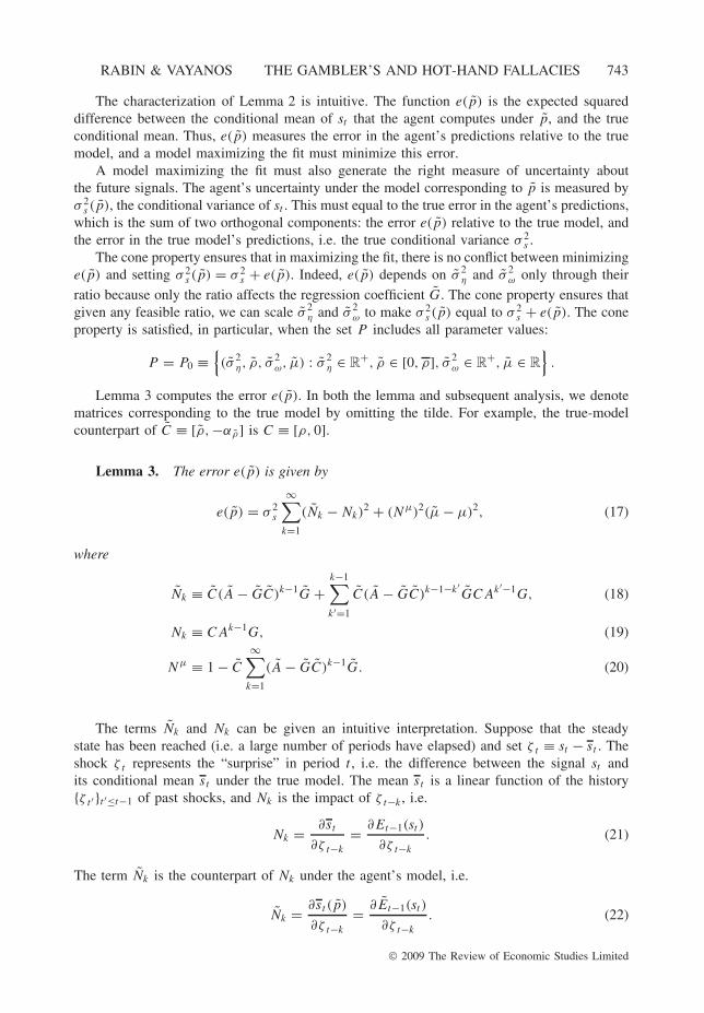
The characterization of Lemma 2 is intuitive. The function e(p) is the expected squareddifference between the conditional mean of st that the agent computes under p, and the trueconditional mean. Thus, e(p) measures the error in the agent’s predictions relative to the truemodel, and a model maximizing the fit must minimize this error.
A model maximizing the fit must also generate the right measure of uncertainty aboutthe future signals. The agent’s uncertainty under the model corresponding to p is measured byσ 2
s (p), the conditional variance of st . This must equal to the true error in the agent’s predictions,which is the sum of two orthogonal components: the error e(p) relative to the true model, andthe error in the true model’s predictions, i.e. the true conditional variance σ 2
s .The cone property ensures that in maximizing the fit, there is no conflict between minimizing
e(p) and setting σ 2s (p) = σ 2
s + e(p). Indeed, e(p) depends on σ 2η and σ 2
ω only through their
ratio because only the ratio affects the regression coefficient G. The cone property ensures thatgiven any feasible ratio, we can scale σ 2
η and σ 2ω to make σ 2
s (p) equal to σ 2s + e(p). The cone
property is satisfied, in particular, when the set P includes all parameter values:
P = P0 ≡{(σ 2
η, ρ, σ 2ω, μ) : σ 2
η ∈ R+, ρ ∈ [0, ρ], σ 2
ω ∈ R+, μ ∈ R
}.
Lemma 3 computes the error e(p). In both the lemma and subsequent analysis, we denotematrices corresponding to the true model by omitting the tilde. For example, the true-modelcounterpart of C ≡ [ρ,−αρ] is C ≡ [ρ, 0].
Lemma 3. The error e(p) is given by
e(p) = σ 2s
∞∑k=1
(Nk − Nk)2 + (Nμ)2(μ − μ)2, (17)
where
Nk ≡ C(A − GC)k−1G +k−1∑k′=1
C(A − GC)k−1−k′GCAk′−1G, (18)
Nk ≡ CAk−1G, (19)
Nμ ≡ 1 − C
∞∑k=1
(A − GC)k−1G. (20)
The terms Nk and Nk can be given an intuitive interpretation. Suppose that the steadystate has been reached (i.e. a large number of periods have elapsed) and set ζ t ≡ st − st . Theshock ζ t represents the “surprise” in period t , i.e. the difference between the signal st andits conditional mean st under the true model. The mean st is a linear function of the history{ζ t ′ }t ′≤t−1 of past shocks, and Nk is the impact of ζ t−k , i.e.
Nk = ∂st
∂ζ t−k
= ∂Et−1(st )
∂ζ t−k
. (21)
The term Nk is the counterpart of Nk under the agent’s model, i.e.
Nk = ∂st (p)
∂ζ t−k
= ∂Et−1(st )
∂ζ t−k
. (22)
© 2009 The Review of Economic Studies Limited
744 REVIEW OF ECONOMIC STUDIES
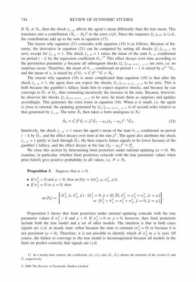
If Nk �= Nk , then the shock ζ t−k affects the agent’s mean differently than the true mean. Thistranslates into a contribution (Nk − Nk)
2 to the error e(p). Since the sequence {ζ t }t∈Z is i.i.d.,the contributions add up to the sum in equation (17).
The reason why equation (21) coincides with equation (19) is as follows. Because of lin-earity, the derivative in equation (21) can be computed by setting all shocks {ζ t ′ }t ′≤t−1 tozero, except for ζ t−k = 1. The shock ζ t−k = 1 raises the mean of the state θ t−k conditionalon period t − k by the regression coefficient G1.17 This effect decays over time according tothe persistence parameter ρ because all subsequent shocks {ζ t ′ }t ′=t−k+1,...,t−1 are zero, i.e. nosurprises occur. Therefore, the mean of θ t−1 conditional on period t − 1 is raised by ρk−1G1,and the mean of st is raised by ρkG1 = CAk−1G = Nk .
The reason why equation (18) is more complicated than equation (19) is that after theshock ζ t−k = 1, the agent does not expect the shocks {ζ t ′ }t ′=t−k+1,...,t−1 to be zero. This isboth because the gambler’s fallacy leads him to expect negative shocks, and because he canconverge to G1 �= G1, thus estimating incorrectly the increase in the state. Because, however,he observes the shocks {ζ t ′ }t ′=t−k+1,...,t−1 to be zero, he treats them as surprises and updatesaccordingly. This generates the extra terms in equation (18). When α is small, i.e. the agentis close to rational, the updating generated by {ζ t ′ }t ′=t−k+1,...,t−1 is of second order relative tothat generated by ζ t−k. The term Nk then takes a form analogous to Nk:
Nk ≈ CAkG = ρkG1 − αρ(δρ − αρ)k−1G2. (23)
Intuitively, the shock ζ t−k = 1 raises the agent’s mean of the state θ t−k conditional on periodt − k by G1, and the effect decays over time at the rate ρk. The agent also attributes the shockζ t−k = 1 partly to luck through G2. He then expects future signals to be lower because of thegambler’s fallacy, and the effect decays at the rate (δρ − αρ)k ≈ δk
ρ.
We close this section by determining limit posteriors under rational updating (α = 0). Weexamine, in particular, whether limit posteriors coincide with the true parameter values whenprior beliefs give positive probability to all values, i.e. P = P0.
Proposition 3. Suppose that α = 0.
• If σ 2η > 0 and ρ > 0, then m(P0) = {(σ 2
η, ρ, σ 2ω, μ)}.
• If σ 2η = 0 or ρ = 0, then
m(P0) ={
(σ 2η, ρ, σ 2
ω, μ) : [σ 2η = 0, ρ ∈ [0, ρ], σ 2
ω = σ 2η + σ 2
ω, μ = μ]or [σ 2
η + σ 2ω = σ 2
η + σ 2ω, ρ = 0, μ = μ]
}.
Proposition 3 shows that limit posteriors under rational updating coincide with the trueparameter values if σ 2
η > 0 and ρ > 0. If σ 2η = 0 or ρ = 0, however, then limit posteriors
include both the true model and a set of other models. The intuition is that in both casessignals are i.i.d. in steady state: either because the state is constant (σ 2
η = 0) or because it isnot persistent (ρ = 0). Therefore, it is not possible to identify which of σ 2
η or ρ is zero. Ofcourse, the failure to converge to the true model is inconsequential because all models in thelimit set predict correctly that signals are i.i.d.
17. In a steady-state context, the coefficients (G1,G2) and (G1, G2) denote the elements of the vectors G andG, respectively.
© 2009 The Review of Economic Studies Limited
RABIN & VAYANOS THE GAMBLER’S AND HOT-HAND FALLACIES 745
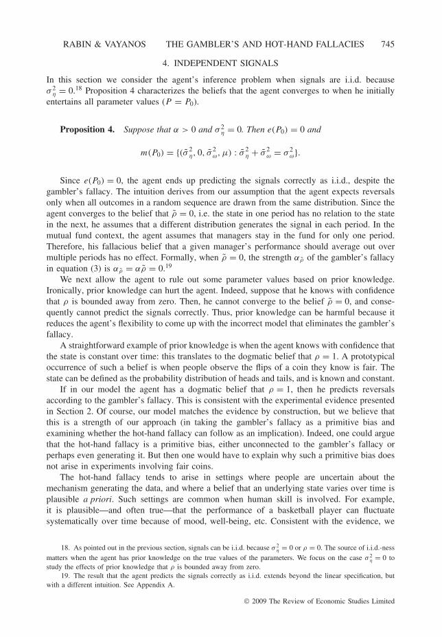
4. INDEPENDENT SIGNALS
In this section we consider the agent’s inference problem when signals are i.i.d. becauseσ 2
η = 0.18 Proposition 4 characterizes the beliefs that the agent converges to when he initiallyentertains all parameter values (P = P0).
Proposition 4. Suppose that α > 0 and σ 2η = 0. Then e(P0) = 0 and
m(P0) = {(σ 2η, 0, σ 2
ω, μ) : σ 2η + σ 2
ω = σ 2ω}.
Since e(P0) = 0, the agent ends up predicting the signals correctly as i.i.d., despite thegambler’s fallacy. The intuition derives from our assumption that the agent expects reversalsonly when all outcomes in a random sequence are drawn from the same distribution. Since theagent converges to the belief that ρ = 0, i.e. the state in one period has no relation to the statein the next, he assumes that a different distribution generates the signal in each period. In themutual fund context, the agent assumes that managers stay in the fund for only one period.Therefore, his fallacious belief that a given manager’s performance should average out overmultiple periods has no effect. Formally, when ρ = 0, the strength αρ of the gambler’s fallacyin equation (3) is αρ = αρ = 0.19
We next allow the agent to rule out some parameter values based on prior knowledge.Ironically, prior knowledge can hurt the agent. Indeed, suppose that he knows with confidencethat ρ is bounded away from zero. Then, he cannot converge to the belief ρ = 0, and conse-quently cannot predict the signals correctly. Thus, prior knowledge can be harmful because itreduces the agent’s flexibility to come up with the incorrect model that eliminates the gambler’sfallacy.
A straightforward example of prior knowledge is when the agent knows with confidence thatthe state is constant over time: this translates to the dogmatic belief that ρ = 1. A prototypicaloccurrence of such a belief is when people observe the flips of a coin they know is fair. Thestate can be defined as the probability distribution of heads and tails, and is known and constant.
If in our model the agent has a dogmatic belief that ρ = 1, then he predicts reversalsaccording to the gambler’s fallacy. This is consistent with the experimental evidence presentedin Section 2. Of course, our model matches the evidence by construction, but we believe thatthis is a strength of our approach (in taking the gambler’s fallacy as a primitive bias andexamining whether the hot-hand fallacy can follow as an implication). Indeed, one could arguethat the hot-hand fallacy is a primitive bias, either unconnected to the gambler’s fallacy orperhaps even generating it. But then one would have to explain why such a primitive bias doesnot arise in experiments involving fair coins.
The hot-hand fallacy tends to arise in settings where people are uncertain about themechanism generating the data, and where a belief that an underlying state varies over time isplausible a priori. Such settings are common when human skill is involved. For example,it is plausible—and often true—that the performance of a basketball player can fluctuatesystematically over time because of mood, well-being, etc. Consistent with the evidence, we
18. As pointed out in the previous section, signals can be i.i.d. because σ 2η = 0 or ρ = 0. The source of i.i.d.-ness
matters when the agent has prior knowledge on the true values of the parameters. We focus on the case σ 2η = 0 to
study the effects of prior knowledge that ρ is bounded away from zero.19. The result that the agent predicts the signals correctly as i.i.d. extends beyond the linear specification, but
with a different intuition. See Appendix A.
© 2009 The Review of Economic Studies Limited
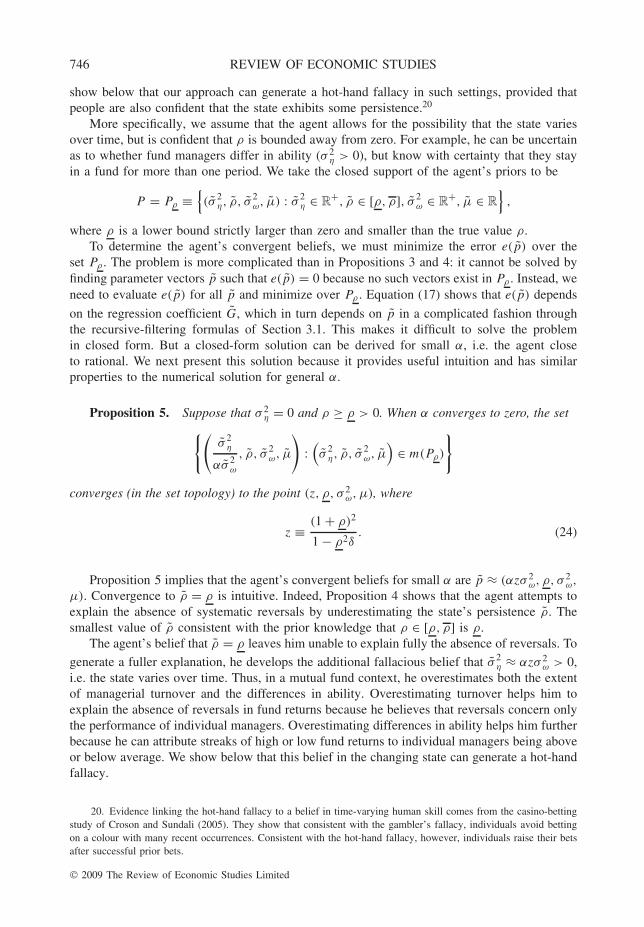
746 REVIEW OF ECONOMIC STUDIES
show below that our approach can generate a hot-hand fallacy in such settings, provided thatpeople are also confident that the state exhibits some persistence.20
More specifically, we assume that the agent allows for the possibility that the state variesover time, but is confident that ρ is bounded away from zero. For example, he can be uncertainas to whether fund managers differ in ability (σ 2
η > 0), but know with certainty that they stayin a fund for more than one period. We take the closed support of the agent’s priors to be
P = Pρ ≡{(σ
2η, ρ, σ
2ω, μ) : σ
2η ∈ R
+, ρ ∈ [ρ, ρ], σ2ω ∈ R
+, μ ∈ R
},
where ρ is a lower bound strictly larger than zero and smaller than the true value ρ.To determine the agent’s convergent beliefs, we must minimize the error e(p) over the
set Pρ . The problem is more complicated than in Propositions 3 and 4: it cannot be solved byfinding parameter vectors p such that e(p) = 0 because no such vectors exist in Pρ . Instead, weneed to evaluate e(p) for all p and minimize over Pρ . Equation (17) shows that e(p) depends
on the regression coefficient G, which in turn depends on p in a complicated fashion throughthe recursive-filtering formulas of Section 3.1. This makes it difficult to solve the problemin closed form. But a closed-form solution can be derived for small α, i.e. the agent closeto rational. We next present this solution because it provides useful intuition and has similarproperties to the numerical solution for general α.
Proposition 5. Suppose that σ 2η = 0 and ρ ≥ ρ > 0. When α converges to zero, the set{(
σ 2η
ασ 2ω
, ρ, σ 2ω, μ
):(σ 2
η, ρ, σ 2ω, μ
)∈ m(Pρ)
}
converges (in the set topology) to the point (z, ρ, σ 2ω, μ), where
z ≡ (1 + ρ)2
1 − ρ2δ. (24)
Proposition 5 implies that the agent’s convergent beliefs for small α are p ≈ (αzσ 2ω, ρ, σ 2
ω,
μ). Convergence to ρ = ρ is intuitive. Indeed, Proposition 4 shows that the agent attempts toexplain the absence of systematic reversals by underestimating the state’s persistence ρ. Thesmallest value of ρ consistent with the prior knowledge that ρ ∈ [ρ, ρ] is ρ.
The agent’s belief that ρ = ρ leaves him unable to explain fully the absence of reversals. To
generate a fuller explanation, he develops the additional fallacious belief that σ 2η ≈ αzσ 2
ω > 0,i.e. the state varies over time. Thus, in a mutual fund context, he overestimates both the extentof managerial turnover and the differences in ability. Overestimating turnover helps him toexplain the absence of reversals in fund returns because he believes that reversals concern onlythe performance of individual managers. Overestimating differences in ability helps him furtherbecause he can attribute streaks of high or low fund returns to individual managers being aboveor below average. We show below that this belief in the changing state can generate a hot-handfallacy.
20. Evidence linking the hot-hand fallacy to a belief in time-varying human skill comes from the casino-bettingstudy of Croson and Sundali (2005). They show that consistent with the gambler’s fallacy, individuals avoid bettingon a colour with many recent occurrences. Consistent with the hot-hand fallacy, however, individuals raise their betsafter successful prior bets.
© 2009 The Review of Economic Studies Limited
RABIN & VAYANOS THE GAMBLER’S AND HOT-HAND FALLACIES 747
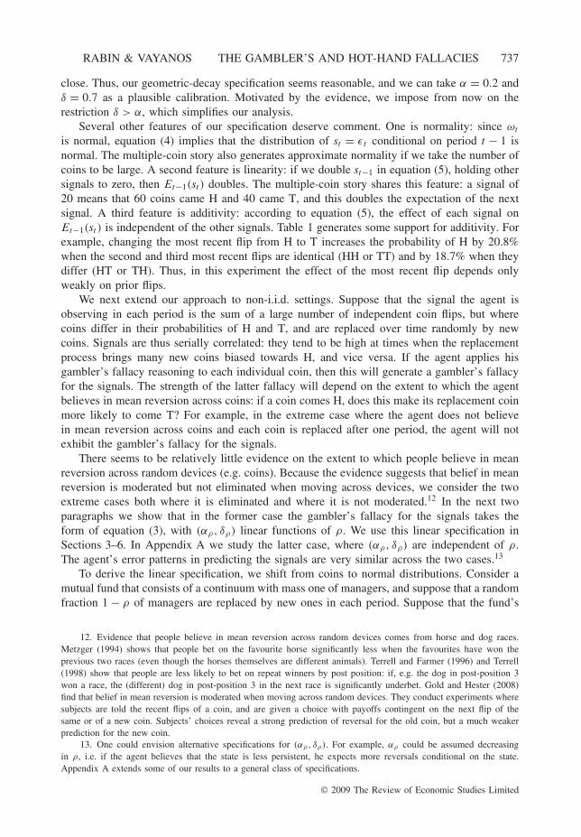
05101520
Ñk
Changing state
Gambler's fallacy
k
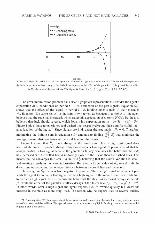
Figure 1Effect of a signal in period t − k on the agent’s expectation Et−1(st ), as a function of k. The dotted line represents
the belief that the state has changed, the dashed line represents the effect of the gambler’s fallacy, and the solid line
is Nk , the sum of the two effects. The figure is drawn for (σ 2η/σ
2ω, ρ, α, δ) = (0, 0.6, 0.2, 0.7)
The error-minimization problem has a useful graphical representation. Consider the agent’sexpectation of st conditional on period t − 1 as a function of the past signals. Equation (22)shows that the effect of the signal in period t − k, holding other signals to their mean, isNk . Equation (23) expresses Nk as the sum of two terms. Subsequent to a high st−k , the agentbelieves that the state has increased, which raises his expectation of st (term ρkG1). But he alsobelieves that luck should reverse, which lowers his expectation (term −αρ(δρ − αρ)k−1G2).Figure 1 plots these terms (dotted and dashed line, respectively) and their sum Nk (solid line),as a function of the lag k.21 Since signals are i.i.d. under the true model, Nk = 0. Therefore,
minimizing the infinite sum in equation (17) amounts to finding( σ 2
η
σ 2ω
, ρ)
that minimize the
average squared distance between the solid line and the x-axis.Figure 1 shows that Nk is not always of the same sign. Thus, a high past signal does
not lead the agent to predict always a high or always a low signal. Suppose instead that healways predicts a low signal because the gambler’s fallacy dominates the belief that the statehas increased (i.e. the dotted line is uniformly closer to the x-axis than the dashed line). Thismeans that he converges to a small value of σ 2
η, believing that the state’s variation is small,
and treating signals as not very informative. But then, a larger value of σ 2η would shift the
dotted line up, reducing the average distance between the solid line and the x-axis.The change in Nk’s sign is from negative to positive. Thus, a high signal in the recent past
leads the agent to predict a low signal, while a high signal in the more distant past leads himto predict a high signal. This is because the belief that the state has increased decays at the rateρk , while the effect of the gambler’s fallacy decays at the faster rate (δρ − αρ)k = ρk(δ − α)k.In other words, after a high signal the agent expects luck to reverse quickly but views theincrease in the state as more long-lived. The reason why he expects luck to reverse quickly
21. Since equation (23) holds approximately, up to second-order terms in α, the solid line is only an approximatesum of the dotted and dashed lines. The approximation error is, however, negligible for the parameter values for whichFigures 1 and 2 are drawn.
© 2009 The Review of Economic Studies Limited
748 REVIEW OF ECONOMIC STUDIES
relative to the state is that he views luck as specific to a given state (e.g. a given fundmanager).
We next draw the implications of our results for the hot-hand fallacy. To define the hot-handfallacy in our model, we consider a streak of identical signals between periods t − k and t − 1,and evaluate its impact on the agent’s expectation of st . Viewing the expectation Et−1(st ) asa function of the history of past signals, the impact is
�k ≡k∑
k′=1
∂Et−1(st )
∂st−k′.
If �k > 0, then the agent expects a streak of k high signals to be followed by a high signal,and vice versa, for a streak of k low signals. This means that the agent expects streaks tocontinue and conforms to the hot-hand fallacy.22
Proposition 6. Suppose that α is small, σ 2η = 0, ρ ≥ ρ > 0, and the agent considers
parameter values in the set Pρ . Then, in steady state, �k is negative for k = 1 and becomespositive as k increases.
Proposition 6 shows that the hot-hand fallacy arises after long streaks while the gambler’sfallacy arises after short streaks. This is consistent with Figure 1 because the effect of a streakis the sum of the effects Nk of each signal in the streak. Since Nk is negative for small k, theagent predicts a low signal following a short streak. But as streak length increases, the positivevalues of Nk overtake the negative values, generating a positive cumulative effect.
Propositions 5 and 6 make use of the closed-form solutions derived for small α. For generalα, the fit-maximization problem can be solved through a simple numerical algorithm and theresults confirm the closed-form solutions: the agent converges to σ 2
η > 0, ρ = ρ, and μ = μ,and his predictions after streaks are as in Proposition 6.23
5. SERIALLY CORRELATED SIGNALS
In this section we relax the assumption that σ 2η = 0, to consider the case where signals are
serially correlated. Serial correlation requires that the state varies over time (σ 2η > 0) and is
persistent (ρ > 0). To highlight the new effects relative to the i.i.d. case, we assume that theagent has no prior knowledge on parameter values.
Recall that with i.i.d. signals and no prior knowledge, the agent predicts correctly becausehe converges to the belief that ρ = 0, i.e. the state in one period has no relation to the state inthe next. When signals are serially correlated, the belief ρ = 0 obviously generates incorrectpredictions. But predictions are also incorrect under a belief ρ > 0 because the gambler’s
22. Our definition of the hot-hand fallacy is specific to streak length, i.e. the agent might conform to the fallacyfor streaks of length k but not k′ �= k. An alternative and closely related definition can be given in terms of the agent’sassessed auto-correlation of the signals. Denote by �k the correlation that the agent assesses between signals k periodsapart. This correlation is closely related to the effect of the signal st−k on the agent’s expectation of st , with the twobeing identical up to second-order terms when α is small. (The proof is available upon request.) Therefore, under theconditions of Proposition 6, the cumulative auto-correlation
∑kk′=1 �k is negative for k = 1 and becomes positive as
k increases. The hot-hand fallacy for lag k can be defined as∑k
k′=1 �k > 0.23. The result that σ 2
η > 0 can be shown analytically. The proof is available upon request.
© 2009 The Review of Economic Studies Limited
RABIN & VAYANOS THE GAMBLER’S AND HOT-HAND FALLACIES 749
fallacy then takes effect. Therefore, there is no parameter vector p ∈ P0 achieving zeroerror e(p).24
We solve the error-minimization problem in closed form for small α and compare with thenumerical solution for general α. In addition to α, we take σ 2
η to be small, meaning that signalsare close to i.i.d. We set ν ≡ σ 2
η/(ασ 2ω) and assume that α and σ 2
η converge to zero holding ν
constant. The case where σ 2η remains constant while α converges to zero can be derived as a
limit for ν = ∞.
Proposition 7. Suppose that ρ > 0. When α and σ 2η converge to zero, holding ν constant,
the set {(σ 2
η
ασ 2ω
, ρ, σ 2ω, μ
):(σ 2
η, ρ, σ 2ω, μ
)∈ m(P0)
}
converges (in the set topology) to the point (z, r, σ 2ω, μ), where
z ≡ νρ(1 − ρ)(1 + r)2
r(1 + ρ)(1 − ρr)+ (1 + r)2
1 − r2δ(25)
and r solves
νρ(1 − ρ)(ρ − r)
(1 + ρ)(1 − ρr)2H1(r) = r2(1 − δ)
(1 − r2δ)2H2(r), (26)
for
H1(r) ≡ νρ(1 − ρ)
(1 + ρ)(1 − ρr)+ r(1 − δ)
[2 − ρr(1 + δ) − r2δ + ρ2r4δ2
](1 − r2δ)2(1 − ρrδ)2
,
H2(r) ≡ νρ(1 − ρ)
(1 + ρ)(1 − ρr)+ r(1 − δ)
(2 − r2δ2 − r4δ3
)(1 − r2δ)(1 − r2δ2)2
.
Because H1(r) and H2(r) are positive, equation (26) implies that r ∈ (0, ρ). Thus, theagent converges to a persistence parameter ρ = r that is between zero and the true value ρ.As in Section 4, the agent underestimates ρ in his attempt to explain the absence of systematicreversals. But he does not converge all the way to ρ = 0 because he must explain the signals’serial correlation. Consistent with intuition, ρ is close to zero when the gambler’s fallacy isstrong relative to the serial correlation (ν small), and is close to ρ in the opposite case.
Consider next the agent’s estimate (1 − ρ)2σ 2η of the variance of the shocks to the state.
Section 4 shows that when σ 2η = 0, the agent can develop the fallacious belief that σ 2
η > 0
24. The proof of this result is available upon request. While models satisfying equations (1) and (2) cannotpredict the signals correctly, models outside that set could. For example, when (αρ, δρ) are independent of ρ, correctpredictions are possible under a model where the state is the sum of two auto-regressive processes: one with persistenceρ1 = ρ, matching the true persistence, and one with persistence ρ2 = δ − α ≡ δ1 − α1, offsetting the gambler’s fallacyeffect. Such a model would not generate correct predictions when (αρ, δρ) are linear in ρ because gambler’s fallacyeffects would decay at the two distinct rates δρi
− αρi= ρi (δ − α) for i = 1, 2. Predictions might be correct, however,
under more complicated models. Our focus is not as much to derive these models, but to characterize the agent’s errorpatterns when inference is limited to a simple class of models that includes the true model.
© 2009 The Review of Economic Studies Limited
750 REVIEW OF ECONOMIC STUDIES
as a way to counteract the effect of the gambler’s fallacy. When σ 2η is positive, we find the
analogous result that the agent overestimates (1 − ρ)2σ 2η. Indeed, he converges to
(1 − ρ)2σ2η ≈ (1 − r)2αzσ 2
ω = (1 − r)2z
(1 − ρ)2ν(1 − ρ)2σ 2
η,
which is larger than (1 − ρ)2σ 2η because of equation (25) and r < ρ. Note that (1 − r)2z is
decreasing in r . Thus, the agent overestimates the variance of the shocks to the state partly asa way to compensate for underestimating the state’s persistence ρ.
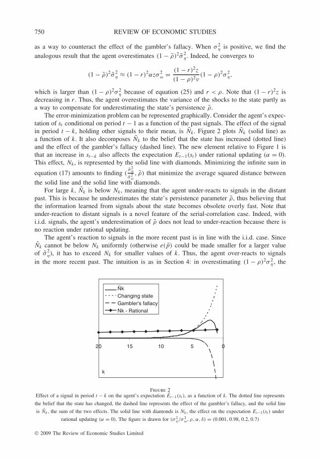
The error-minimization problem can be represented graphically. Consider the agent’s expec-tation of st conditional on period t − 1 as a function of the past signals. The effect of the signalin period t − k, holding other signals to their mean, is Nk . Figure 2 plots Nk (solid line) asa function of k. It also decomposes Nk to the belief that the state has increased (dotted line)and the effect of the gambler’s fallacy (dashed line). The new element relative to Figure 1 isthat an increase in st−k also affects the expectation Et−1(st ) under rational updating (α = 0).This effect, Nk , is represented by the solid line with diamonds. Minimizing the infinite sum in
equation (17) amounts to finding (σ 2
η
σ 2ω
, ρ) that minimize the average squared distance between
the solid line and the solid line with diamonds.For large k, Nk is below Nk , meaning that the agent under-reacts to signals in the distant
past. This is because he underestimates the state’s persistence parameter ρ, thus believing thatthe information learned from signals about the state becomes obsolete overly fast. Note thatunder-reaction to distant signals is a novel feature of the serial-correlation case. Indeed, withi.i.d. signals, the agent’s underestimation of ρ does not lead to under-reaction because there isno reaction under rational updating.
The agent’s reaction to signals in the more recent past is in line with the i.i.d. case. SinceNk cannot be below Nk uniformly (otherwise e(p) could be made smaller for a larger valueof σ 2
η), it has to exceed Nk for smaller values of k. Thus, the agent over-reacts to signalsin the more recent past. The intuition is as in Section 4: in overestimating (1 − ρ)2σ 2
η, the
05101520
ÑkChanging stateGambler's fallacyNk - Rational
k
Figure 2Effect of a signal in period t − k on the agent’s expectation Et−1(st ), as a function of k. The dotted line represents
the belief that the state has changed, the dashed line represents the effect of the gambler’s fallacy, and the solid line
is Nk , the sum of the two effects. The solid line with diamonds is Nk , the effect on the expectation Et−1(st ) under
rational updating (α = 0). The figure is drawn for (σ 2η/σ
2ω, ρ, α, δ) = (0.001, 0.98, 0.2, 0.7)
© 2009 The Review of Economic Studies Limited
RABIN & VAYANOS THE GAMBLER’S AND HOT-HAND FALLACIES 751
agent exaggerates the signals’ informativeness about the state. Finally, the agent under-reactsto signals in the very recent past because of the gambler’s fallacy.
We next draw the implications of our results for predictions after streaks. We consider astreak of identical signals between periods t − k and t − 1, and evaluate its impact on theagent’s expectation of st , and on the expectation under rational updating. The impact for theagent is �k, and that under rational updating is
�k ≡k∑
k′=1
∂Et−1(st )
∂st−k′.
If �k > �k , then the agent expects a streak of k high signals to be followed by a higher signalthan under rational updating, and vice versa for a streak of k low signals. This means that theagent over-reacts to streaks.
Proposition 8. Suppose that α and σ 2η are small, ρ > 0, and the agent has no prior
knowledge (P = P0). Then, in steady state �k − �k is negative for k = 1, becomes positive ask increases, and then becomes negative again.
Proposition 8 shows that the agent under-reacts to short streaks, over-reacts to longerstreaks, and under-reacts to very long streaks. The under-reaction to short streaks is because ofthe gambler’s fallacy. Longer streaks generate over-reaction because the agent overestimatesthe signals’ informativeness about the state. But he also underestimates the state’s persistence,thus under-reacting to very long streaks.
The numerical results for general α confirm most of the closed-form results. The onlyexception is that Nk − Nk can change sign only once, from positive to negative. Under-reactionthen occurs only to very long streaks. This tends to happen when the agent underestimates thestate’s persistence significantly (because α is large relative to σ 2
η). As a way to compensate for
his error, he overestimates (1 − ρ)2σ 2η significantly, viewing signals as very informative about
the state. Even very short streaks can then lead him to believe that the change in the state islarge and dominates the effect of the gambler’s fallacy.
We conclude this section by summarizing the main predictions of the model. Thesepredictions could be tested in controlled experimental settings or in field settings. Prediction 1follows from our specification of the gambler’s fallacy.
Prediction 1 When individuals observe i.i.d. signals and are told this information, theyexpect reversals after streaks of any length. The effect is stronger for longer streaks.
Predictions 2 and 3 follow from the results of Sections 4 and 5. Both predictions requireindividuals to observe long sequences of signals so that they can learn sufficiently about thesignal-generating mechanism.
Prediction 2 Suppose that individuals observe i.i.d. signals, but are not told this informa-tion, and do not exclude on prior grounds the possibility that the underlying distribution mightbe changing over time. Then, a belief in continuation of streaks can arise. Such a belief shouldbe observed following long streaks, while belief in reversals should be observed following shortstreaks. Both beliefs should be weaker if individuals believe on prior grounds that the underlyingdistribution might be changing frequently.
Prediction 3 Suppose that individuals observe serially correlated signals. Then, relative tothe rational benchmark, they over-react to long streaks, but under-react to very long streaksand possibly to short ones as well.
© 2009 The Review of Economic Studies Limited
752 REVIEW OF ECONOMIC STUDIES
6. FINANCE APPLICATIONS
In this section we explore the implications of our model for financial decisions. Our goalis to show that the gambler’s fallacy can have a wide range of implications, and that ournormal-linear model is a useful tool for pursuing them.
6.1. Active investing
A prominent puzzle in finance is why people invest in actively managed funds in spite of theevidence that these funds underperform their passively managed counterparts. This puzzle hasbeen documented by academics and practitioners, and has been the subject of two presidentialaddresses to the American Finance Association (Gruber, 1996; French, 2008). Gruber (1996)finds that the average active fund underperforms its passive counterpart by 35–164 basis points(bps, hundredths of a percent) per year. French (2008) estimates that the average investor wouldsave 67 bps per year by switching to a passive fund. Yet, despite this evidence, passive fundsrepresent only a small minority of mutual fund assets.25
Our model can help explain the active-fund puzzle. We interpret the signal as the return ona traded asset (e.g. a stock), and the state as the expected return. Suppose that expected returnsare constant because σ 2
η = 0, and so returns are i.i.d. Suppose also that an investor prone to thegambler’s fallacy is uncertain about whether expected returns are constant, but is confident thatif expected returns do vary, they are serially correlated (ρ > 0). Section 4 then implies that theinvestor ends up believing in return predictability. The investor would therefore be willing topay for information on past returns, while such information has no value under rational updating.
Turning to the active-fund puzzle, suppose that the investor is unwilling to continuouslymonitor asset returns, but believes that market experts observe this information. Then, hewould be willing to pay for experts’ opinions or for mutual funds operated by the experts.The investor would thus be paying for active funds in a world where returns are i.i.d. andactive funds have no advantage over passive funds. In summary, the gambler’s fallacy canhelp explain the active-fund puzzle because it can generate an incorrect and confident beliefthat active managers add value.26,27
We illustrate our explanation with a simple asset-market model, to which we return inSection 6.2. Suppose that there are N stocks, and the return on stock n = 1, . . . , N in periodt is snt . The return on each stock is generated by equations (1) and (2). The parameter σ 2
η
is equal to zero for all stocks, meaning that returns are i.i.d. over time. All stocks have the
25. Gruber (1996) finds that the average active fund investing in stocks underperforms the market by 65–194bps per year, where the variation in estimates is due to different methods of risk adjustment. He compares theseestimates to an expense ratio of 30 bps for passive funds. French (2008) aggregates the costs of active strategies overall stock market participants (mutual funds, hedge funds, institutional asset management, etc.) and finds that they are79 bps, while the costs of passive strategies are 12 bps. Bogle (2005) reports that passive funds represent one-seventhof mutual fund equity assets as of 2004.
26. Our explanation of the active-fund puzzle relies not on the gambler’s fallacy per se, but on the more generalnotion that people recognize deterministic patterns in random data. We are not aware of models of false patternrecognition that pursue the themes in this section.
27. Identifying the value added by active managers with their ability to observe past returns can be criticized onthe grounds that past returns can be observed at low cost. Costs can, however, be large when there is a large numberof assets, as in the model that we consider next. Stepping slightly outside of the model, suppose that the investor isconfident that random data exhibit deterministic patterns, but does not know what the exact patterns are. (In our modelthis would mean that the investor is confident that signals are predictable, but does not know the model parameters.)Then, the value added by active managers would derive not only from their ability to observe past returns, but alsofrom their knowledge of the patterns.
© 2009 The Review of Economic Studies Limited
RABIN & VAYANOS THE GAMBLER’S AND HOT-HAND FALLACIES 753
same expected return μ and variance σ 2ε , and are independent of each other. An active-fund
manager chooses an all-stock portfolio in each period by maximizing expected return subject toa tracking-error constraint. This constraint requires that the standard deviation of the manager’sreturn relative to the equally weighted portfolio of all stocks does not exceed a bound T E.Constraints of this form are common in asset management (e.g. Roll, 1992). We denote byst ≡ ∑N
n=1 snt /N the return on the equally weighted portfolio of all stocks.The investor starts with the prior knowledge that the persistence parameter associated to
each stock exceeds a bound ρ > 0. He observes a long history of stock returns that endsin the distant past. This leads him to the limit posteriors on model parameters derived inSection 4. The investor does not observe recent returns. He assumes, however, that the managerhas observed the entire return history, has learned about model parameters in the same wayas him, and interprets recent returns in light of these estimates. We denote by E and Var ,respectively, the manager’s expectation and variance operators, as assessed by the investor.The variance Vart−1(snt ) is independent of t in steady state, and independent of n becausestocks are symmetric. We denote it by Var1.
The investor is aware of the manager’s objective and constraints. He assumes that in periodt the manager chooses portfolio weights {wnt }n=1,...,N to maximize the expected return
Et−1
(N∑
n=1
wntsnt
)(27)
subject to the tracking error constraint
Vart−1
(N∑
n=1
wntsnt − st
)≤ TE2, (28)
and the constraint that weights sum to 1,∑N
n=1 wnt = 1.
Lemma 4. The manager’s maximum expected return, as assessed by the investor, is
Et−1(st ) + TE√Var1
√√√√ N∑n=1
[Et−1(snt ) − Et−1(st )
]2. (29)
According to the investor, the manager’s expected return exceeds that of a passive fundholding the equally weighted portfolio of all stocks. The manager adds value because ofher information, as reflected in the cross-sectional dispersion of return forecasts. When thedispersion is large, the manager can achieve high expected return because her portfolio differssignificantly from equal weights. The investor believes that the manager’s forecasts shouldexhibit dispersion because the return on each stock is predictable on the basis of the stock’spast history.
6.2. Fund flows
Closely related to the active-fund puzzle is a puzzle concerning fund flows. Flows into mutualfunds are strongly positively correlated with the funds’ lagged returns (e.g. Chevalier andEllison, 1997; Sirri and Tufano, 1998), and yet lagged returns do not appear to be strong
© 2009 The Review of Economic Studies Limited
754 REVIEW OF ECONOMIC STUDIES
predictors of future returns (e.g. Carhart, 1997).28 Ideally, the fund-flow and active-fund puzzlesshould be addressed together within a unified setting: explaining flows into active funds raisesthe question why people invest in these funds in the first place.
To study fund flows, we extend the asset-market model of Section 6.1, allowing the investorto allocate wealth over an active and a passive fund. The passive fund holds the equallyweighted portfolio of all stocks and generates return st . The active fund’s return is st + γt . Ina first step, we model the excess return γt in reduced form, without reference to the analysisof Section 6.1: we assume that γt is generated by equations (1) and (2) for values of (σ 2
η, σ2ε)
denoted by (σ 2ηγ, σ
2εγ), γt is i.i.d. because σ 2
ηγ = 0, and γt is independent of st . Under theseassumptions, the investor’s beliefs about γt can be derived as in Section 4. In a second step,we use the analysis of Section 6.1 to justify some of the assumed properties of γt , and moreimportantly to derive additional properties.
We modify slightly the model of Section 6.1 by replacing the single infinitely lived investorwith a sequence of generations. Each generation consists of one investor, who invests over oneperiod and observes all past information. This simplifies the portfolio problem, rendering itmyopic, while the inference problem remains as with a single investor.
Investors observe the history of returns of the active and the passive fund. Their portfolioallocation decision, derived below, depends on their beliefs about the excess return γt of theactive fund. Investors believe that γt is generated by equations (1) and (2), is independent of st ,and its persistence parameter exceeds a bound ρ
γ> 0. After observing a long history of fund
returns, investors converge to the limit posteriors on model parameters derived in Section 4.The investor entering the market in period t starts with wealth W , and derives utility over
final wealth Wt . To keep with the normal-linear structure, we take utility to be exponentialwith coefficient of absolute risk aversion a. The investor chooses portfolio weight wt in theactive fund to maximize the expected utility
−Et−1 exp(−aWt )
subject to the budget constraint
Wt = W[(1 − wt )(1 + st ) + wt (1 + st + γt )
]= W
[(1 + st ) + wtγt
].
Because of normality and exponential utility, the problem is mean-variance. Independencebetween st and γt implies that the solution is
wt = Et−1(γt )
aW Var1γ
,
where Var1γ ≡ Vart−1(γt ) and Var denotes the variance assessed by the investor. (The varianceVart−1(γt ) is independent of t in steady state.) The optimal investment in the active fund is alinear increasing function of the investor’s expectation of the fund’s excess return γt . The net
28. Similar findings exist for hedge funds. See, for example, Ding et al. (2008) and Fung et al. (2008). Berkand Green (2004) propose a rational explanation for the fund-flow puzzle. They assume that ability differs acrossmanagers and can be inferred from fund returns. Able managers perform well and receive inflows, but because ofdecreasing returns to managing a large fund, their performance drops to that of average managers. Their model doesnot explain the active-fund puzzle, nor does it fully address the origin of decreasing returns.
© 2009 The Review of Economic Studies Limited
RABIN & VAYANOS THE GAMBLER’S AND HOT-HAND FALLACIES 755
flow into the active fund in period t + 1 is the change in investment between periods t andt + 1:
Ft+1 ≡ W wt+1 − W wt = Et (γt+1) − Et−1(γt )
aVar1γ
. (30)
Lemma 5 determines the covariance between returns and subsequent flows.
Lemma 5. The covariance between the excess return of the active fund in period t andthe net flow into the fund during periods t + 1 through t + k for k ≥ 1 is
Cov
(γt ,
k∑k′=1
Ft+k′
)= σ 2
εγNk
aVar1γ
. (31)
where Nk is defined by equation (22), with γt replacing st .
Recall from Section 4 (e.g. Figure 1) that Nk is negative for small k and becomes positiveas k increases. Hence, returns are negatively correlated with subsequent flows when flows aremeasured over a short horizon, and are positively correlated over a long horizon. The negativecorrelation is inconsistent with the evidence on the fund-flow puzzle. It arises because investorsattribute high returns partly to luck, and expecting luck to reverse, they reduce their investmentin the fund. Investors also develop a fallacious belief that high returns indicate high managerialability, and this tends to generate positive performance–flow correlation, consistent with theevidence. But the correlation cannot be positive over all horizons because the belief in abilityarises to offset but not to overtake the gambler’s fallacy.
We next use the analysis of Section 6.1 to derive properties of the active fund’s excessreturn γt . Consider first properties under the true model. Since the returns on all stocks areidentical and constant over time, all active portfolios achieve zero excess return. The manageris thus indifferent over portfolios, and we assume that he selects one meeting the tracking-errorconstraint [equation (28)] with equality.29 Therefore, conditional on past history, γt is normalwith mean zero and variance σ 2
εγ = TE2. Since the mean and variance do not depend on pasthistory, γt is i.i.d. Moreover, γt is uncorrelated with st because
Covt−1(γt , st ) = Covt−1
(N∑
n=1
wntsnt − st , st
)= σ 2
ε
(∑Nn=1 wn,t
N− 1
N
)= 0,
where the second step follows because stocks are symmetric and returns are uncorrelated.Consider next properties of γt as assessed by the investor. Since the investor believes that the
active manager adds value, γt has positive mean. Moreover, this mean varies over time and isserially correlated. Indeed, recall from Lemma 4 that the active fund’s expected excess return,as assessed by the investor, is increasing in the cross-sectional dispersion of the manager’sreturn forecasts. This cross-sectional dispersion varies over time and is serially correlated: it issmall, for example, when stocks have similar return histories since these histories are used togenerate the forecasts.
29. We assume that the manager is rational and operates under the true model. The manager has a strict preferencefor a portfolio meeting equation (28) with equality if returns are arbitrarily close to i.i.d.
© 2009 The Review of Economic Studies Limited
756 REVIEW OF ECONOMIC STUDIES
Time variation in the mean of γt implies that the value added by the manager is time-varying, i.e. σ 2
ηγ > 0. Section 4 derives belief in time-varying managerial ability as a posteriorto which the investor converges after observing a long history of fund returns. This sectionshows instead that such a belief can arise without observation of fund returns, and as aconsequence of the investor’s belief in the power of active management. This belief can actas a prior when the investor observes fund returns, and can lead to inferences different than inSection 4. Indeed, suppose that the investor believes on prior grounds that σ 2
ηγ exceeds a boundσ 2
ηγ > 0. If the convergent posterior in the absence of this prior knowledge is smaller than σ 2ηγ,
then prior knowledge implies convergence to σ 2ηγ instead. As a consequence, the fallacious
belief that high returns indicate high managerial ability becomes stronger and could generatepositive performance–flow correlation over any horizon, consistent with the fund-flow puzzle.
A problem with our analysis is that when stock returns are normal (as in Section 6.1), fundreturns, as assessed by the investor, are non-normal. This is because the mean of γt depends onthe cross-sectional dispersion of stock return forecasts, which is always positive and thus non-normal. Despite this limitation, we believe that the main point is robust: a fallacious belief thatactive managers add value gives rise naturally to a belief that the added value varies over time,in a way that can help explain the fund-flow puzzle. Belief in time variation could arise throughthe cross-sectional dispersion of the manager’s return forecasts. Alternatively, it could arisebecause of an assumed dispersion in ability across managers, e.g. only some managers collectinformation on past returns and make good forecasts according to the investor. Neither of thetwo mechanisms would generate time variation under the true model because past returns donot forecast future returns. Put differently, a rational investor who knows that active managersdo not add value would also rule out the possibility that the added value varies over time.
We illustrate our analysis with a numerical example. We assume that the investor observesfund returns once a year. We set ρ
γ= 0.6, i.e. at least 60% of managerial ability carries over
to the next year. We set the tracking error TE = 5%. We follow the calibration of Section 2and set the parameters of the gambler’s fallacy α = 0.2 and δ = 0.7. Section 4 then impliesthat in the absence of prior knowledge on σηγ, the investor converges to σ ηγ = 3.66%. He thusbelieves that managers performing one standard deviation above average beat those performingone standard deviation below by 7.32% per year.
Can prior knowledge lead to the belief that σηγ exceeds σ ηγ? Suppose, for example, thatthere are two types of managers: those collecting information on past returns and those who donot. A manager collecting no information achieves zero expected excess return. To derive theexpected excess return, as assessed by the investor, of a manager collecting information, wemake the following assumptions. There are N = 50 stocks, and the manager observes stockreturns and makes trades once a month. We set ρ = 0.8, i.e. at least 80% of a shock to astock’s expected return carries over to the next month. For large N , the expected excess returnin Lemma 4 becomes approximately
TE√Var1
√NVar
[Et−1(snt )
]. (32)
The ratio√
Var[Et−1(snt )]/Var1 is 9.97%, meaning that the cross-sectional dispersion of themanager’s return forecasts is 9.97% of her estimate of the standard deviation of each stock.Since we are evaluating returns at a monthly frequency, we set TE = 5%/
√12. Substituting
into equation (32), we find that the manager’s expected excess return is 0.77% per month, i.e.9.23% per year. Assuming that managers of the two types are equally likely, this translates toa standard deviation in managerial ability of 4.62% per year. This is larger than σ ηγ = 3.66%.
© 2009 The Review of Economic Studies Limited
RABIN & VAYANOS THE GAMBLER’S AND HOT-HAND FALLACIES 757
Adding the prior knowledge that σηγ ≥ 4.62% to the analysis of Section 4 yields a positiveperformance–flow correlation over any horizon, consistent with the fund-flow puzzle.
While flows in the numerical example respond positively to returns over any horizon, theresponse is strongest over intermediate horizons. This reflects the pattern derived in Section 4(e.g. Figure 1), with the difference that the Nk-curve is positive even for small k. Of course,the delayed reaction of flows to returns could arise for reasons other than the gambler’s fallacy,e.g. costs of adjustment.
6.3. Equilibrium
Sections 6.1 and 6.2 take stock returns as given. A comprehensive analysis of the generalequilibrium effects that would arise if investors prone to the gambler’s fallacy constitute alarge fraction of the market is beyond the scope of this paper. Nonetheless, some implicationscan be sketched.
Suppose that investors observe a stock’s i.i.d. normal dividends. Suppose, as in Section 6.2,that investors form a sequence of generations, each investing over one period and maximizingexponential utility. Suppose finally that investors are uncertain about whether expecteddividends are constant, but are confident that if expected dividends do vary, they are seriallycorrelated (ρ > 0). If investors are rational, they would learn that dividends are i.i.d., andequilibrium returns would also be i.i.d.30 If, instead, investors are prone to the gambler’sfallacy, returns would exhibit short-run momentum and long-run reversal. Intuitively, sinceinvestors expect a short streak of high dividends to reverse, the stock price under-reacts to thestreak. Therefore, a high return is, on average, followed by a high return, implying short-runmomentum. Since, instead, investors expect a long streak of high dividends to continue, thestock price over-reacts to the streak. Therefore, a sequence of high returns is, on average,followed by a low return, implying long-run reversal and a value effect. These results aresimilar to Barberis, Shleifer and Vishny (1998), although the mechanism is different.
A second application concerns trading volume. Suppose that all investors are subject tothe gambler’s fallacy, but observe different subsets of the return history. Then, they wouldform different forecasts for future dividends. If, in addition, prices are not fully revealing (e.g.because of noise trading), then investors would trade because of the different forecasts. Nosuch trading would occur under rational updating, and therefore the gambler’s fallacy wouldgenerate excessive trading.
APPENDIX A. ALTERNATIVE SPECIFICATIONS FOR (αρ, δρ)
Consider first the case where signals are i.i.d. because σ 2η = 0, and the agent initially entertains all parameter
values. Under the constant specification, where (αρ, δρ) are independent of ρ and equal to (α, δ) ≡ (α1, δ1),Proposition 4 is replaced by
Proposition A1. Suppose that α > 0 and σ 2η = 0. Then e(P0) = 0, and m(P0) consists of the two elements
p1 ≡(
α(1 − δ2 + δα)
δ(1 − δ + α)2σ 2
ω, δ − α,δ − α
δσ 2
ω, μ
)and
p2 ≡ (σ 2ω, 0, 0, μ).
30. Proofs of all results in this section are available upon request.
© 2009 The Review of Economic Studies Limited
758 REVIEW OF ECONOMIC STUDIES
As in Proposition 4, the agent ends up predicting the signals correctly as i.i.d., despite the gambler’s fallacy.Correct predictions can be made using either of two models. Under model p1, the agent believes that the state θ t variesover time and is persistent. The state’s persistence parameter ρ is equal to the decay rate δ − α > 0 of the gambler’sfallacy effect. (Decay rates are derived in (23).) This ensures that the agent’s updating on the state can exactly offsethis belief that luck should reverse. Under model p2, the agent attributes all variation in the signal to the state, andsince the gambler’s fallacy applies only to the sequence {εt }t≥1, it has no effect.
Proposition 4 can be extended to a broader class of specifications. Suppose that the function ρ ∈ [0, 1] → δρ − αρ
crosses the 45-degree line at a single point ρ ∈ [0, 1). Then, the agent ends up predicting the signals correctly as i.i.d.,i.e. e(P0) = 0, and m(P0) consists of the element p2 of Proposition A1 and an element p1 for which ρ = ρ. Underthe linear specification, ρ = 0, and under the constant specification, ρ = δ − α.
Consider next the case where the agent is confident that ρ is bounded away from zero, and the closed support ofhis priors is P = Pρ . Under the constant specification, Proposition 6 is replaced by:
Proposition A2. Suppose that α is small, σ 2η = 0, ρ ≥ ρ > δ, and the agent considers parameter values in the
set Pρ . Then, in steady state �k is negative for k = 1 and becomes positive as k increases.
As in Proposition 6, the hot-hand fallacy arises after long streaks of signals while the gambler’s fallacy arisesafter short streaks. Note that Proposition A2 requires the additional condition ρ > δ. If instead ρ < δ, then the agentpredicts the signals correctly as i.i.d. Indeed, because ρ < δ − α for small α, model p1 of Proposition A1 belongs toPρ (provided that ρ is close to one so that ρ > δ), and therefore, e(Pρ) = 0 and m(Pρ) = {p1}. Proposition A2 canbe extended to the broader class of specifications defined above, with the condition ρ > δ replaced by ρ > ρ.
Consider finally the case where signals are serially correlated. Under the constant specification, Proposition 8 isreplaced by:
Proposition A3. Suppose that α and σ 2η are small, ρ /∈ {0, δ}, the agent has no prior knowledge (P = P0), and
one of the following is met
2ρ
1 + ρ2> δ, (A1)
ν2ρ4(1 − ρ)(1 − δ2)
(1 + ρ)3> 1. (A2)
Then, in steady state �k − �k is negative for k = 1, becomes positive as k increases, and then becomes negative again.
As in Proposition 8, the agent under-reacts to short streaks, over-reacts to longer streaks, and under-reacts to very
long streaks. Proposition A3 is, in a sense, stronger than Proposition 8 because it derives the under/over/under-reaction
pattern regardless of whether ρ is larger or smaller than δ. (The relevant comparison in Proposition 8 is between ρ
and zero.) The agent converges to a value ρ between ρ and δ. When ρ > δ, the under-reaction to very long streaks
is because the agent underestimates the state’s persistence. When instead ρ < δ, the agent overestimates the state’s
persistence, and the under-reaction to very long streaks is due to the large memory parameter δ of the gambler’s
fallacy. Conditions (A1) and (A2) ensure that when α and σ 2η are small, in which case the agent converges to a model
predicting signals close to i.i.d., it is σ 2η rather than ρ that is small. A small-ρ model predicts signals close to i.i.d.
for the same reason as model p2 of Proposition A1: because variation in the signal is mostly attributed to the state.
Appendix B shows that when the gambler’s fallacy applies to both {εt }t≥1 and {ηt }t≥1, a model similar to p1 becomes
the unique element of m(P0) in the setting of Proposition A1, and conditions (A1) and (A2) are not needed in the
setting of Proposition A3.
APPENDIX B. GAMBLER’S FALLACY FOR THE STATE
Our model and solution method can be extended to the case where the gambler’s fallacy applies to both thesequence {εt }t≥1 that generates the signals given the state, and the sequence {ηt }t≥1 that generates the state. Suppose
© 2009 The Review of Economic Studies Limited

RABIN & VAYANOS THE GAMBLER’S AND HOT-HAND FALLACIES 759
that according to the agent,
ηt = ζ t − α
∞∑k=0
δkηt−1−k, (B1)
where the sequence {ζ t }t≥1 is i.i.d. normal with mean zero and variance σ 2ζ . To formulate the recursive-filtering
problem, we expand the state vector to
xt ≡ [θ t − μ, εδ
t , ηδt
]′,
where
ηδt ≡
∞∑k=0
δkηt−k.
We also set
A ≡⎡⎣ ρ 0 −(1 − ρ)α
0 δρ − αρ 00 0 δ − α
⎤⎦ ,
wt ≡ [(1 − ρ)ζ t , ωt , ζ t ]′,
C ≡ [ρ,−αρ,−(1 − ρ)α],
vt ≡ (1 − ρ)ζ t + ωt , and p ≡ (σ 2ζ , ρ, σ 2
ω, μ). Under these definitions, the analysis of the agent’s inference in Section 3carries through identical.
When signals are i.i.d. because σ 2η = 0, and the agent initially entertains all parameter values, his limit posteriors
are as follows:
Proposition B1. Suppose that α > 0 and σ 2η = 0. If (αρ, δρ) = (αρ, δρ), then e(P0) = 0 and
m(P0) = {(0, 0, σ 2ω, μ)}.
If (αρ, δρ) = (α, δ), then e(P0) = 0 and
m(P0) ={(
α(1 − δ2 + δα)
δ(1 − δ)2σ 2
ω, δ,δ − α
δσ 2
ω, μ
)}.
Under both the linear and the constant specification, the agent ends up predicting the signals correctly as i.i.d.Therefore, the main result of Propositions 4 and A1 extends to the case where the gambler’s fallacy applies to both{εt }t≥1 and {ηt }t≥1. The set of models that yield correct predictions, however, becomes a singleton. The only modelunder the linear specification is one in which the state is constant, and the only model under the constant specificationis one similar to model p1 of Proposition A1.
When the agent is confident that ρ is bounded away from zero, he ends up believing that σ 2η > 0. When, in
addition, α is small, so is σ 2η. Therefore, the effects of the gambler’s fallacy for {ηt }t≥1 are small relative to {εt }t≥1,
and the analysis is the same as when the gambler’s fallacy applies only to {εt }t≥1. In particular, the agent’s predictionsafter streaks are as in Propositions 6 and A2.
Consider finally the case where signals are serially correlated. When α and σ 2η are small, the agent converges
to a model where σ 2η is small. (Unlike with Proposition A3, Conditions (A1) and (A2) are not needed to rule out
the small-ρ model.) Therefore, the effects of the gambler’s fallacy for {ηt }t≥1 are small relative to {εt }t≥1, and theanalysis is the same as when the gambler’s fallacy applies only to {εt }t≥1. In particular, the agent’s predictions afterstreaks are as in Propositions 8 and A3.
© 2009 The Review of Economic Studies Limited

760 REVIEW OF ECONOMIC STUDIES
APPENDIX C. PROOFS
Proof of Proposition 1. Our formulation of the recursive-filtering problem is as in standard textbooks. Forexample, equations (8) and (9) follow from (4.1.1) and (4.1.4) in Balakrishnan (1987) if xn+1 is replaced by xt , xn
by xt−1, An by A, Un by 0, Nsn by wt , vn by st − μ, Cn by C, and N0
n by vt . Equation (10) follows from (4.6.14), ifthe latter is written for n + 1 instead of n, and xn+1 is replaced by xt , xn by xt−1, and AKn + Qn by Gt . That Gt
so defined is given by equation (12) follows from (4.1.29) and (4.6.12) if Hn−1 is replaced by �t−1, GnG′n by V ,
and Jn by U . Equation (11) follows from (4.6.18) if the latter is written for n + 1 instead of n, Pn is substituted from(4.1.30), and FnF
′n is replaced by W . ‖
Proof of Proposition 2. It suffices to show (Balakrishnan, pp. 182–184) that the eigenvalues of A − U V −1C
have modulus smaller than 1. This matrix is⎡⎢⎢⎣
σ2ω
(1−ρ)2 σ2η+σ2
ωρ
(1−ρ)2 σ2η
(1−ρ)2 σ2η+σ2
ωαρ
− σ2ω
(1−ρ)2 σ2η+σ2
ωρ δρ − (1−ρ)2 σ2
η
(1−ρ)2 σ2η+σ2
ωαρ
⎤⎥⎥⎦ .
The characteristic polynomial is
λ2 − λ
[σ 2
ω
(1 − ρ)2σ 2η + σ 2
ω
ρ + δρ − (1 − ρ)2σ 2η
(1 − ρ)2σ 2η + σ 2
ω
αρ
]+ σ 2
ω
(1 − ρ)2σ 2η + σ 2
ω
ρδρ
≡ λ2 − λb + c
Suppose that the roots λ1, λ2 of this polynomial are real, in which case λ1 + λ2 = b and λ1λ2 = c. Since c > 0, λ1
and λ2 have the same sign. If λ1 and λ2 are negative, they are both greater than −1, since b > −1 from αρ < 1 andρ, δρ ≥ 0. If λ1 and λ2 are positive, then at least one is smaller than 1, since b < 2 from ρ, δρ < 1 and αρ ≥ 0. Butsince the characteristic polynomial for λ = 1 takes the value
(1 − δρ)
[1 − σ 2
ω
(1 − ρ)2σ 2η + σ 2
ω
ρ
]+ (1 − ρ)2σ 2
η
(1 − ρ)2σ 2η + σ 2
ω
αρ > 0,
both λ1 and λ2 are smaller than 1. Suppose instead that λ1, λ2 are complex. In that case, they are conjugates and themodulus of each is
√c < 1. ‖
Lemma C1 determines st , the true mean of st conditional on Ht−1, and st (p), the mean that the agent computesunder the parameter vector p. To state the lemma, we set ζ t ≡ st − st , Dt ≡ A − Gt C, D ≡ A − GC, and
Jt,t ′ ≡{∏t
k=t ′ Dk for t ′ = 1, . . . , t ,
I for t ′ > t .
For simplicity, we set the initial condition x0 = 0.
Lemma C1. The true mean st is given by
st = μ +t−1∑t ′=1
CAt−t ′−1Gt ′ζ t ′ (C1)
and the agent’s mean st (p) by
st (p) = μ +t−1∑t ′=1
CMt,t ′ζ t ′ + CMμt (μ − μ), (C2)
where
Mt,t ′ ≡ Jt−1,t ′+1Gt ′ +t−1∑
k=t ′+1
Jt−1,k+1GkCAk−t ′−1Gt ′ ,
Mμt ≡
t−1∑t ′=1
Jt−1,t ′+1Gt ′ .
© 2009 The Review of Economic Studies Limited

RABIN & VAYANOS THE GAMBLER’S AND HOT-HAND FALLACIES 761
Proof. Consider the recursive-filtering problem under the true model, and denote by xt the true mean of xt .Equation (9) implies that
st = μ + Cxt−1. (C3)
Equation (10) then implies that
xt = Axt−1 + Gt(st − st ) = Axt−1 + Gtζ t .
Iterating between t − 1 and zero, we find
xt−1 =t−1∑t ′=1
At−t ′−1Gt ′ζ t ′ . (C4)
Plugging into equation (C3), we find equation (C1).Consider next the agent’s recursive-filtering problem under p. Equation (10) implies that
xt (p) = (A − Gt C)xt−1(p) + Gt (st − μ).
Iterating between t − 1 and zero, we find
xt−1(p) =t−1∑t ′=1
Jt−1,t ′+1Gt ′ (st ′ − μ) (C5)
=t−1∑t ′=1
Jt−1,t ′+1Gt ′ (ζ t ′ + μ − μ + Cxt ′−1),
where the second step follows from st ′ = ζ t ′ + st ′ and equation (C3). Substituting xt ′−1 from equation (C4), andgrouping terms, we find
xt−1(p) =t−1∑t ′=1
Mt,t ′ζ t ′ + Mμt (μ − μ). (C6)
Combining this with
st (p) = μ + Cxt−1(p) (C7)
(which follows from equation (9)), we find equation (C2). ‖We next prove Lemma 3. While this Lemma is stated after Theorem 1 and Lemmas 1 and 2, its proof does not
rely on these results.
Proof of Lemma 3. Lemma C1 implies that
st (p) − st =t−1∑t ′=1
et,t ′ζ t ′ + Nμt (μ − μ), (C8)
where
et,t ′ ≡ CMt,t ′ − CAt−t ′−1Gt ′ ,
Nμt ≡ 1 − CM
μt .
Therefore,
[st (p) − st ]2 =
t−1∑t ′,t ′′=1
et,t ′et,t ′′ζ t ′ζ t ′′ + (Nμt )2(μ − μ)2 + 2
t−1∑t ′=1
et,t ′Nμt ζ t ′ (μ − μ). (C9)
© 2009 The Review of Economic Studies Limited

762 REVIEW OF ECONOMIC STUDIES
Since the sequence {ζ t ′ }t ′=1,...,t−1 is independent under the true measure and mean-zero, we have
E[st (p) − st
]2 =t−1∑t ′=1
e2t,t ′σ
2s,t ′ + (N
μt )2(μ − μ)2. (C10)
We first determine the limit of∑t−1
t ′=1 e2t,t ′σ
2s,t ′ when t goes to ∞. Defining the double sequence {φk,t }k,t≥1 by
φk,t ≡{
e2t,t−kσ
2s,t−k for k = 1, . . . , t − 1,
0 for k > t − 1,,
we have
t−1∑t ′=1
e2t,t ′σ
2s,t ′ =
t−1∑k=1
e2t,t−kσ
2s,t−k =
∞∑k=1
φk,t .
The definitions of et,t ′ and Mt,t ′ imply that
et,t−k = CJt−1,t−k+1Gt−k +k−1∑k′=1
CJt−1,t−k+k′+1Gt−k+k′CAk′−1Gt−k − CAk−1Gt−k. (C11)
Equation (9) applied to the recursive-filtering problem under the true model implies that
σ 2s,t = C�t−1C
′ + V.
When t goes to ∞, Gt goes to G, Gt to G, �t to �, and Jt,t−k to Dk+1. Therefore,
limt→∞ et,t−k = CDk−1G +
k−1∑k′=1
CDk−1−k′ GCAk′−1G − CAk−1G = Nk − Nk ≡ ek,
limt→∞ σ 2
s,t−k = C�C ′ + V = C�C ′ + (1 − ρ)2σ 2η + σ 2
ω = σ 2s , (C12)
implying that
limt→∞ φk,t = e2
kσ2s .
The dominated convergence theorem will imply that
limt→∞
∞∑k=1
φk,t =∞∑
k=1
limt→∞ φk,t = σ 2
s
∞∑k=1
e2k , (C13)
if there exists a sequence {φk}k≥1 such that∑∞
k=1 φk < ∞ and |φk,t | ≤ φk for all k, t ≥ 1. To construct such asequence, we note that the eigenvalues of A have modulus smaller than 1, and so do the eigenvalues of D ≡ A − GC
(Balakrishnan, Theorem 4.2.3, p. 111). Denoting by a < 1 a number exceeding the maximum of the moduli, we canconstruct a dominating sequence {φk}k≥1 decaying geometrically at the rate a2k .
We next determine the limit of Nμt . Defining the double sequence {χk,t }k,t≥1 by
χk,t ≡{
Jt−1,t−k+1Gt−k for k = 1, . . . , t − 1,
0 for k > t − 1,
we have
Nμt = 1 − C
t−1∑k=1
Jt−1,t−k+1Gt−k = 1 − C
∞∑k=1
χk,t .
© 2009 The Review of Economic Studies Limited
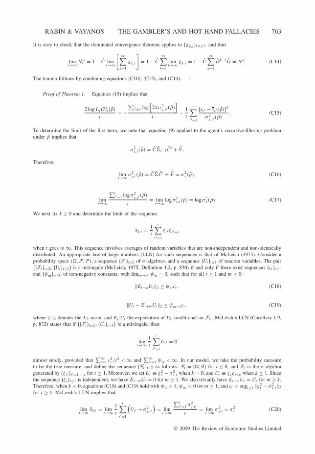
RABIN & VAYANOS THE GAMBLER’S AND HOT-HAND FALLACIES 763
It is easy to check that the dominated convergence theorem applies to {χk,t }k,t≥1, and thus
limt→∞ N
μt = 1 − C lim
t→∞
[ ∞∑k=1
χk,t
]= 1 − C
∞∑k=1
limt→∞ χk,t = 1 − C
∞∑k=1
Dk−1G = Nμ. (C14)
The lemma follows by combining equations (C10), (C13), and (C14). ‖
Proof of Theorem 1. Equation (15) implies that
2 log Lt(Ht |p)
t= −
∑tt ′=1 log
[2πσ 2
s,t ′ (p)]
t− 1
t
t∑t ′=1
[st ′ − st ′ (p)]2
σ 2s,t ′ (p)
. (C15)
To determine the limit of the first term, we note that equation (9) applied to the agent’s recursive-filtering problemunder p implies that
σ 2s,t (p) = C�t−1C
′ + V .
Therefore,
limt→∞ σ 2
s,t (p) = C�C ′ + V = σ 2s (p), (C16)
limt→∞
∑tt ′=1 log σ 2
s,t ′ (p)
t= lim
t→∞ log σ 2s,t (p) = log σ 2
s (p). (C17)
We next fix k ≥ 0 and determine the limit of the sequence
Sk,t ≡ 1
t
t∑t ′=1
ζ t ′ζ t ′+k
when t goes to ∞. This sequence involves averages of random variables that are non-independent and non-identicallydistributed. An appropriate law of large numbers (LLN) for such sequences is that of McLeish (1975). Consider aprobability space (�,F, P ), a sequence {Ft }t∈Z of σ -algebras, and a sequence {Ut }t≥1 of random variables. The pair({Ft }t∈Z, {Ut }t≥1
)is a mixingale (McLeish, 1975, Definition 1.2, p. 830) if and only if there exist sequences {ct }t≥1
and {ψm}m≥0 of non-negative constants, with limm→∞ ψm = 0, such that for all t ≥ 1 and m ≥ 0:
‖Et−mUt‖2 ≤ ψmct , (C18)
‖Ut − Et+mUt‖2 ≤ ψm+1ct , (C19)
where ‖.‖2 denotes the L2 norm, and Et ′Ut the expectation of Ut conditional on Ft ′ . McLeish’s LLN (Corollary 1.9,p. 832) states that if
({Ft }t∈Z, {Ut }t≥1)
is a mixingale, then
limt→∞
1
t
t∑t ′=1
Ut ′ = 0
almost surely, provided that∑∞
t=1 c2t /t2 < ∞ and
∑∞m=1 ψm < ∞. In our model, we take the probability measure
to be the true measure, and define the sequence {Ft }t∈Z as follows: Ft = {�,∅} for t ≤ 0, and Ft is the σ -algebragenerated by {ζ t ′ }t ′=1,...,t for t ≥ 1. Moreover, we set Ut ≡ ζ 2
t − σ 2s,t when k = 0, and Ut ≡ ζ t ζ t+k when k ≥ 1. Since
the sequence {ζ t }t≥1 is independent, we have Et−mUt = 0 for m ≥ 1. We also trivially have Et+mUt = Ut for m ≥ k.Therefore, when k = 0, equations (C18) and (C19) hold with ψ0 = 1, ψm = 0 for m ≥ 1, and ct = supt≥1 ‖ζ 2
t − σ 2s,t‖2
for t ≥ 1. McLeish’s LLN implies that
limt→∞ S0,t = lim
t→∞1
t
t∑t ′=1
(Ut ′ + σ 2
s,t ′)
= limt→∞
∑tt ′=1 σ 2
s,t ′t
= limt→∞ σ 2
s,t = σ 2s (C20)
© 2009 The Review of Economic Studies Limited

764 REVIEW OF ECONOMIC STUDIES
almost surely. When k ≥ 1, equations (C18) and (C19) hold with ψm = 1 for m = 0, . . . , k − 1, ψm = 0 for m ≥ k,and ct = supt≥1 ‖ζ t‖2
2 for t ≥ 1. McLeish’s LLN implies that
limt→∞ Sk,t = lim
t→∞1
t
t∑t ′=1
Ut ′ = 0 (C21)
almost surely. Finally, a straightforward application of McLeish’s LLN to the sequence Ut ≡ ζ t implies that
limt→∞
1
t
t∑t ′=1
ζ t ′ = 0 (C22)
almost surely. Since N is countable, we can assume that equations (C20), (C21) for all k ≥ 1, and equation (C22),hold in the same measure-one set. In what follows, we consider histories in that set.To determine the limit of the second term in equation (C15), we write it as
1
t
t∑t ′=1
ζ 2t ′
σ 2s,t ′ (p)︸ ︷︷ ︸
Xt
− 2
t
t∑t ′=1
ζ t ′ [st ′ (p) − st ′ ]σ 2
s,t ′ (p)︸ ︷︷ ︸Yt
+ 1
t
t∑t ′=1
[st ′ (p) − st ′ ]2
σ 2s,t ′ (p)︸ ︷︷ ︸
Zt
.
Since limt→∞ σ 2s,t (p) = σ 2
s (p), we have
limt→∞ Xt = 1
σ 2s (p)
limt→∞
1
t
t∑t ′=1
ζ 2t ′ = 1
σ 2s (p)
limt→∞ S0,t = σ 2
s
σ 2s (p)
. (C23)
Using equation (C8), we can write Yt as
Yt = 2∞∑
k=1
ψk,t + 2
t
t∑t ′=1
Nμ
t ′σ 2
s,t ′ (p)ζ t ′ (μ − μ),
where the double sequence {ψk,t }k,t≥1 is defined by
ψk,t ≡⎧⎨⎩
1t
∑tt ′=k+1
et ′,t ′−k
σ2s,t ′ (p)
ζ t ′ζ t ′−k for k = 1, . . . , t − 1,
0 for k > t − 1.
Since limt→∞ et,t−k = ek and limt→∞ Nμt = Nμ, we have
limt→∞ ψk,t = ek
σ 2s (p)
limt→∞
1
t
t∑t ′=k+1
ζ t ′ζ t ′−k = ek
σ 2s (p)
limt→∞ Sk,t = 0,
limt→∞
1
t
t∑t ′=1
Nμ
t ′σ 2
s,t ′ (p)ζ t ′ (μ − μ) = Nμ
σ 2s (p)
(μ − μ) limt→∞
1
t
t∑t ′=1
ζ t ′ = 0.
The dominated convergence theorem will imply that
limt→∞ Yt = 2 lim
t→∞
∞∑k=1
ψk,t = 2∞∑
k=1
limt→∞ ψk,t = 0 (C24)
if there exists a sequence {ψk}k≥1 such that∑∞
k=1 ψk < ∞ and |ψk,t | ≤ ψk for all k, t ≥ 1. Such a sequence can beconstructed by the same argument as for φk,t (Lemma 3) since∣∣∣∣∣∣
1
t
t∑t ′=k+1
ζ t ′ζ t ′−k
∣∣∣∣∣∣ ≤ 1
t
t∑t ′=k+1
∣∣ζ t ′∣∣ ∣∣ζ t ′−k
∣∣ ≤√√√√ 1
t
t∑t ′=k+1
ζ 2t ′
√√√√ 1
t
t∑t ′=k+1
ζ 2t ′−k
≤ supt≥1
S0,t < ∞,
where the last inequality holds because the sequence S0,t is convergent.
© 2009 The Review of Economic Studies Limited

RABIN & VAYANOS THE GAMBLER’S AND HOT-HAND FALLACIES 765
Using similar arguments as for Yt , we find
limt→∞ Zt = σ 2
s
σ 2s (p)
∞∑k=1
e2k + (Nμ)2
σ 2s (p)
(μ − μ)2 = e(p)
σ 2s (p)
. (C25)
The theorem follows from equations (C15), (C17), (C23), (C24), and (C25). ‖
Proof of Lemma 1. We first show that the set m(P ) is non-empty. Equation (C16) implies that when σ 2η or σ 2
ω
go to ∞, σ 2s (p) goes to ∞ and F(p) goes to −∞. Therefore, we can restrict the maximization of F(p) to bounded
values of (σ 2η, σ 2
ω). Equation (20) implies that
Nμ = 1 − C(I − D)−1G = 1 − C(I − A + GC)−1G.
Replacing A and C by their values, and denoting the components of G by G1 and G2, we find
Nμ = 1 − C(I − A + GC)−1G = (1 − ρ)(1 − δρ + αρ)
[1 − ρ(1 − G1)](1 − δρ + αρ) − αρ(1 − ρ)G2. (C26)
Since αρ, δρ ∈ [0, 1) and ρ ∈ [0, ρ], Nμ �= 0. Therefore, when |μ| goes to ∞, Lemma 3 implies that e(p) goes to∞ and F(p) goes to −∞. This means that we can restrict the maximization of F(p) to bounded values of μ, andthus to a compact subset of P . We can also assume that F(p) is continuous in that subset since the only point ofdiscontinuity is for σ 2
s (p) = 0, in which case F(p) = −∞. Therefore, F(p) has a maximum and the set m(P ) isnon-empty.
To show that the measure πt converges weakly to a measure giving weight only to m(P ), it suffices to showthat for all closed sets S having zero intersection with m(P ), πt (S) goes to zero (Billingsley, 1986, Theorem 29.1, p.390). The maximum FS of F(p) over S is the same as in a compact subset of S and is thus smaller than the value ofF(p) in m(P ). Consider a compact neighbourhood B of a point in m(P ) such that the minimum FB of F(p) over B
exceeds FS . Consider also two constants (F1, F2) such that FB > F2 > F1 > FS . For large enough t ,
minp∈B
log Lt(Ht |p)
t> F2. (C27)
Indeed, if equation (C27) does not hold, there exists a convergent sequence {pt }t≥1 in B such that
log Lt (Ht |pt )
t≤ F2.
Denoting the limit of this sequence by p ∈ B, Theorem 1 implies that F(p) ≤ F2, a contradiction. (Theorem 1concerns the convergence of the likelihood for a given p, but extending the argument to a convergent sequence{pt }t≥1 is straightforward.) Likewise, we can show that for large enough t ,
maxp∈S
log Lt(Ht |p)
t< F1. (C28)
Bayes’ law, equation (C27), and equation (C28) imply that for large enough t ,
πt (S) = Eπ0
[Lt(Ht |p)1{p∈S}
]Eπ0
[Lt(Ht |p)
] <Eπ0
[Lt (Ht |p)1{p∈S}
]Eπ0
[Lt(Ht |p)1{p∈B}
] <exp(tF1)π0(S)
exp(tF2)π0(B).
Since F2 > F1, πt (S) goes to zero when t goes to ∞. ‖
Proof of Lemma 2. Consider p ∈ P such that e(p) = e(P ) and σ 2s (p) = σ 2
s + e(p). We will show thatF(p) ≥ F(p) for any p = (σ
2η, ρ, σ
2ω, μ) ∈ P . Denote by � and G the steady-state variance and regression coefficient
for the recursive-filtering problem under p, and by �λ and Gλ those under pλ ≡ (λσ2η, ρ, λσ
2ω, μ) for λ > 0. It is
easy to check that λ� solves equation (13) for pλ. Since this equation has a unique solution, �λ = λ�. Equation (12)then implies that Gλ = G, and equations (17) and (C16) imply that e(pλ) = e(p) and σ 2
s (pλ) = λσ 2s (p). Therefore,
F(pλ) = − 1
2
[log[2πλσ 2
s (p)]+ σ 2
s + e(p)
λσ 2s (p)
]. (C29)
© 2009 The Review of Economic Studies Limited

766 REVIEW OF ECONOMIC STUDIES
Since this function is maximized for
λ∗ = σ 2s + e(p)
σ 2s (p)
,
we have
F(p) ≤ F(pλ∗ ) = − 1
2
[log[2π[σ 2
s + e(p)]]+ 1
] ≤ − 1
2
[log[2π[σ 2
s + e(p)]]+ 1
] = F(p).
The proof of the converse is along the same lines. ‖Lemma C2 determines when a model can predict the signals equally well as the true model.
Lemma C2. The error e(p) is zero if and only if
• CAk−1G = CAk−1G for all k ≥ 1
• μ = μ.
Proof. From Lemma 3 and Nμ �= 0, it suffices to show that {ek}k≥1 = 0 is equivalent to CAk−1G = CAk−1G
for all k ≥ 1. Setting ak ≡ CAk−1G − CAk−1G and
bk ≡ Dk−1G +k−1∑k′=1
Dk−1−k′ GCAk′−1G − Ak−1G,
we have ek = Cbk + ak for k ≥ 1. Simple algebra shows that
bk = Dbk−1 − Gak−1.
Iterating between k and 1, and using the initial condition b1 = 0, we find
bk = −k−1∑k′=1
Dk−1−k′ Gak′ .
Therefore,
ek = −k−1∑k′=1
CDk−1−k′ Gak′ + ak. (C30)
Equation (C30) implies that {ek}k≥1 = 0 if and only if {ak}k≥1 = 0. ‖
Proof of Proposition 3. Under rational updating, it is possible to achieve minimum error e(P0) = 0 by usingthe vector of true parameters p. Since e(P0) = 0, Lemmas 2 and C2 imply that p ∈ m(P0) if and only if (i)CAk−1G = CAk−1G for all k ≥ 1, (ii) μ = μ, and (iii) σ 2
s (p) = σ 2s . Since α = 0, we can write Condition (i) as
ρkG1 = ρkG1. (C31)
We can also write element (1,1) of equation (13) as
�11 =[ρ2�11 + (1 − ρ)2σ 2
η
]σ 2
ω
ρ2�11 + (1 − ρ)2σ 2η + σ 2
ω
, (C32)
�11 =[ρ2�11 + (1 − ρ)2σ 2
η
]σ 2
ω
ρ2�11 + (1 − ρ)2σ 2η + σ 2
ω
, (C33)
and the first element of equation (14) as
G1 = ρ2�11 + (1 − ρ)2σ 2η
ρ2�11 + (1 − ρ)2σ 2η + σ 2
ω
, (C34)
G1 = ρ2�11 + (1 − ρ)2σ 2η
ρ2�11 + (1 − ρ)2σ 2η + σ 2
ω
, (C35)
© 2009 The Review of Economic Studies Limited

RABIN & VAYANOS THE GAMBLER’S AND HOT-HAND FALLACIES 767
where the first equation in each case is for p and the second for p. Using equations (C12) and (C16), we can writeCondition (iii) as
ρ2�11 + (1 − ρ)2σ 2η + σ 2
ω = ρ2�11 + (1 − ρ)2σ 2η + σ 2
ω. (C36)
Suppose that ρσ 2η > 0, and consider p that satisfies Conditions (i)–(iii). Equation (C35) implies that G1 > 0.
Since equation (C31) must hold for all k ≥ 1, we have ρ = ρ and G1 = G1. We next write equations (C32)–(C35)in terms of the normalized variables s2
η ≡ σ 2η/σ
2ω, S11 ≡ �11/σ
2ω , s2
η ≡ σ 2η/σ
2ω, and S11 ≡ �11/σ
2ω. Equations (C32)
and (C33) imply that S11 = g(s2η) and S11 = g(s2
η) for the same function g. Equations (C34), (C35), and G1 = G1
then imply that s2η = s2
η , and equation (C36) implies that σ 2ω = σ 2
ω. Thus, p = p.Suppose next that ρσ 2
η = 0, and consider p that satisfies Conditions (i)–(iii). If ρ = 0, equation (C31) implies that
ρkG1 = 0, and equation (C36) that ρ2�11 + (1 − ρ)2σ 2η + σ 2
ω = σ 2η + σ 2
ω. If σ 2η = 0, the same implications follow
because � = 0 and G = [0, 1]′ from equations (13) and (14). Equation ρkG1 = 0 implies that either ρ = 0, or G1 = 0in which case σ 2
η = 0. If ρ = 0, then σ 2η + σ 2
ω = σ 2η + σ 2
ω. If σ 2η = 0, then σ 2
ω = σ 2η + σ 2
ω. Therefore, p is as in theproposition. Showing that all p in the proposition satisfy Conditions (i)–(iii) is obvious. ‖
Proof of Proposition 4. We determine the parameter vectors p that belong to m(P0) and satisfy e(p) = 0. FromLemmas 2 and C2, these must satisfy (i) CAk−1G = CAk−1G for all k ≥ 1, (ii) μ = μ, and (iii) σ 2
s (p) = σ 2s . Since
σ 2η = 0, we can write Condition (i) as
ρkG1 − αρ(δρ − αρ)k−1G2 = 0, (C37)
and Condition (iii) as
C�C ′ + V = σ 2ω. (C38)
Using (αρ , δρ ) = (αρ, δρ), we can write equation (C37) as
ρk[G1 − α(δ − α)k−1G2
]= 0. (C39)
If ρ �= 0, equation (C39) implies that G1 − α(δ − α)k−1G2 = 0 for all k ≥ 1, which in turn implies that G = 0. ForG = 0, equation (13) becomes � = A�A′ + W . Solving for �, we find
�11 = (1 − ρ)σ 2η
1 + ρ,
�12 = 0,
�22 = σ 2ω
1 − (δρ − αρ)2.
Substituting � into equation (14), we find (σ 2η, σ
2ω) = 0. But then, � = 0, which contradicts equation (C38) since
σ 2ω = σ 2
ε > 0. Therefore, ρ = 0. Equation (C38) then implies that σ 2η + σ 2
ω = σ 2ω . Showing that all p in the proposition
satisfy Conditions (i)–(iii) is obvious. ‖
Proof of Proposition 5. Consider a sequence {αn}n∈N converging to zero, and an element pn ≡ ((σ 2η)n, ρn, (σ
2ω)n,
μn) from the set m(Pρ) corresponding to αn. The proposition will follow if we show that ((s2
η)n
αn, ρn, (σ
2ω)n, μn)
converges to (z, ρ, σ 2ω, μ), where (s2
η)n ≡ (σ 2η)n/(σ
2ω)n. Denoting the limits of (
(s2η)n
αn, (σ 2
η)n, ρn, (σ2ω)n, μn) by
( s, η, ρ, ω, μ), the point ( η, ρ, ω, μ) belongs to the set m(Pρ) derived for α = σ 2η = 0. (If the sequences
do not converge, we extract converging subsequences.) All elements in that set satisfy μ = μ. Proposition 3 impliesthat they also satisfy σ 2
η = 0 and σ 2ω = σ 2
ω since ρ ≥ ρ > 0. Therefore, ( μ, η, ω) = (μ, 0, σ 2ω).
When v ≡ (α,s2ηα
, σ 2η, ρ, σ 2
ω) converges to v ≡ (0, s , 0, ρ , σ 2ω), CDkG converges to zero,
G1s2η
to1− ρ1+ ρ
, and
G2 to 1. These limits follow by continuity if we show that when α = σ 2η = 0, CDkG = 0 and G2 = 1, and when
α = 0, limσ2η→0
G1s2η
= 1−ρ
1+ρ. When σ 2
η = 0, the unique solution of equation (13) is � = 0, and equation (14) implies
that G = [0, 1]′. Therefore, when α = σ 2η = 0, we have CG = 0,
CD = C(A − GC) = CA = ρC,
© 2009 The Review of Economic Studies Limited

768 REVIEW OF ECONOMIC STUDIES
and CDkG = ρkCG = 0. Moreover, if we divide both sides of equations (C32) and (C34) (derived from equations(13) and (14) when α = 0) by σ 2
ω , we find
S11 = ρ2S11 + (1 − ρ)2 s2η
ρ2S11 + (1 − ρ)2 s2η + 1
, (C40)
G1 = ρ2S11 + (1 − ρ)2 s2η
ρ2S11 + (1 − ρ)2 s2η + 1
. (C41)
When σ 2η converges to zero, s2
η and S11 converge to zero. Equations (C40) and (C41) then imply thatS11s2η
andG1s2η
converge to 1−ρ1+ρ
.Using the above limits, we find
limv→ v
CAk−1G
α= lim
v→ v
ρkG1 − αρ(δρ − αρ)k−1G2
α
= limv→ v
ρk
[s2η
α
G1
s2η
− (δ − α)k−1G2
]= k
ρ
[ s(1 − ρ)
1 + ρ
− δk−1]
.
Equations (18), (C30), limv→ v CDkG = 0, and Nk = CAkG = 0, imply that
limv→ v
ek
α= lim
v→ v
Nk
α= lim
v→ v
CDk−1G
α= lim
v→ v
ak
α= lim
v→ v
CAk−1G
α= k
ρ
[ s(1 − ρ)
1 + ρ
− δk−1]
. (C42)
Since pn minimizes e(pn), equation (17) implies that ((σ 2η)n, ρn, (σ
2ω)n) minimizes σ 2
s (p)∑∞
k=0 e2k . Since from
equation (C42),
limv→ v
σ 2s (p)
∑∞k=1 e2
k
α2= σ 2
ω
∞∑k=1
2kρ
[ s(1 − ρ)
1 + ρ
− δk−1]2
≡ σ 2ωF ( s, ρ),
( s , ρ) must minimize F . Treating F as a function of(
s (1− ρ )
1+ ρ, ρ
), the minimizing value of the second argument
is clearly ρ = ρ. The first-order condition with respect to the first argument is
∞∑k=1
2kρ
[ s(1 − ρ)
1 + ρ
− δk−1]
= 0. (C43)
Substituting ρ = ρ into equation (C43), we find s = z. ‖
Proof of Proposition 6. Equations (C5) and (C7) imply that in steady state
Et−1(st ) ≡ st (p) = μ +∞∑
k=1
CDk−1G(st−k − μ). (C44)
Therefore,
�k =k∑
k′=1
CDk′−1G.
Equation (C42) implies that
�k = αgk + o(α),
where
gk ≡k∑
k′=1
fk′ ,
fk ≡ ρk
[z(1 − ρ)
1 + ρ− δk−1
].
© 2009 The Review of Economic Studies Limited

RABIN & VAYANOS THE GAMBLER’S AND HOT-HAND FALLACIES 769
Using equation (24) to substitute z, we find
f1 = g1 = ρ3(δ − 1)
1 − ρ2δ< 0,
g∞ = ρ
[z
1 + ρ− 1
1 − ρδ
]= ρ2(1 − δ)
(1 − ρ2δ)(1 − ρδ)> 0.
The function fk is negative for k = 1 and positive for large k. Since it can change sign only once, it is negativeand then positive. The function gk is negative for k = 1, then decreases (fk < 0), then increases (fk > 0), and iseventually positive (g∞ > 0). Therefore, gk is negative and then positive. ‖
Proof of Proposition 7. Consider a sequence {αn}n∈N converging to zero, an element pn ≡ ((σ 2η)n, ρn, (σ
2ω)n, μn)
from the set m(P0) corresponding to αn, and set (σ 2η)n ≡ ναnσ
2ω. The proposition will follow if we show
that ((s2
η)n
αn, ρn, (σ
2ω)n, μn) converges to (z, r, σ 2
ω, μ). Denoting the limits of ((s2
η)n
αn, (σ 2
η)n, ρn, (σ2ω)n, μn) by
( s, η, ρ, ω, μ), the point ( η, ρ, ω, μ) belongs to the set m(P0) derived for α = σ 2η = 0. Proposition 3 implies
that μ = μ. If ρ > 0, then Proposition 3 implies also that ( η, ω) = (0, σ 2ω), and same arguments as in the proof
of Proposition 5 imply that
limv→ v
σ 2s (p)
∑∞k=1 e2
k
α2= σ 2
ω
∞∑k=1
( kρ
[ s(1 − ρ)
1 + ρ
− δk−1]
− ρk ν(1 − ρ)
1 + ρ
)2
≡ σ 2ωH( s , ρ).
If ρ = 0, then the limit is instead
limv→ v
σ 2s (p)
∑∞k=1 e2
k
α2= σ 2
ω
([ φ − ρ
ν(1 − ρ)
1 + ρ
]2
+∞∑
k=2
[ρk ν(1 − ρ)
1 + ρ
]2)
≡ σ 2ωH0( φ),
where φ denotes the limit of ρn(G1)nαn
. The cases ρ > 0 and ρ = 0 can be nested by noting that H0( φ) is equal
to H evaluated for s ρ = φ and ρ = 0. Treating H as a function of(
s (1− ρ )
1+ ρ, ρ
), the first-order condition with
respect to the first argument is
∞∑k=1
kρ
( kρ
[ s(1 − ρ)
1 + ρ
− δk−1]
− ρk ν(1 − ρ)
1 + ρ
)= 0, (C45)
and the derivative with respect to the second argument is
∞∑k=1
k k−1ρ
[ s(1 − ρ)
1 + ρ
− δk−1](
kρ
[ s(1 − ρ)
1 + ρ
− δk−1]
− ρk ν(1 − ρ)
1 + ρ
). (C46)
Computing the infinite sums, we can write equation (C45) as
s ρ
(1 + ρ)2− ρ
1 − 2ρδ
− νρ(1 − ρ)
(1 + ρ)(1 − ρ ρ)= 0 (C47)
and equation (C46) as
s(1 − ρ)
1 + ρ
[ s ρ
(1 + ρ)2(1 − 2ρ)
− ρ
(1 − 2ρδ)2
− νρ(1 − ρ)
(1 + ρ)(1 − ρ ρ)2
]
−[
s ρ(1 − ρ)
(1 + ρ)(1 − 2ρδ)2
− ρ
(1 − 2ρδ2)2
− νρ(1 − ρ)
(1 + ρ)(1 − ρ ρδ)2
]. (C48)
Substituting s from equation (C47), we can write the first square bracket in equation (C48) as
− νρ(1 − ρ) ρ(ρ − ρ)
(1 + ρ)(1 − ρ ρ)2(1 − 2ρ)
+ 3ρ(1 − δ)
(1 − 2ρ)(1 − 2
ρδ)
© 2009 The Review of Economic Studies Limited

770 REVIEW OF ECONOMIC STUDIES
and the second as
νρ(1 − ρ) ρ(ρ − ρ)[1 − 2δ + (ρ + ρ) ρδ2 − ρ 3
ρδ2]
(1 + ρ)(1 − ρ ρ)(1 − 2ρδ)2(1 − ρ ρδ)2
− 3ρ(1 − δ)
[1 − 2δ + 2
ρ(1 + δ)δ2 − 4ρδ3]
(1 − 2ρδ)3(1 − 2
ρδ2)2.
We next substitute s from equation (C47) into the term s (1− ρ )
1+ ρthat multiplies the first square bracket in equation
(C48). Grouping terms, we can write equation (C48) as
− νρ(1 − ρ)(ρ − ρ)
(1 + ρ)(1 − ρ ρ)2H1( ρ) + 2
ρ(1 − δ)
(1 − 2ρδ)2
H2( ρ). (C49)
The functions H1( ρ) and H2( ρ) are positive for ρ ∈ [0, ρ] because
2 − ρ ρ(1 + δ) − 2ρδ + ρ2 4
ρδ2 > 0, (C50)
2 − 2ρδ2 − 4
ρδ3 > 0. (C51)
(To show equations (C50) and (C51), we use ρ, δ < 1. For equation (C50) we also note that the left-hand side isdecreasing in δ and positive for δ = 1.) Since H1( ρ),H2( ρ) > 0, equation (C49) is negative for ρ = 0 and positivefor ρ ∈ [ρ, ρ]. Therefore, the value of ρ that minimizes H is in (0, ρ) and renders equation (C49) equal to zero.Comparing equations (26) and (C49), we find that this value is equal to r . Substituting ρ = r into equation (C47),we find s = z. ‖
Proof of Proposition 8. Proceeding as in the proof of Proposition 6, we find
�k − �k = αgk + o(α),
where
gk ≡k∑
k′=1
fk′ ,
fk ≡ rk
[z(1 − r)
1 + r− δk−1
]− ρk ν(1 − ρ)
1 + ρ. (C52)
The proposition will follow if we show that f1 = g1 < 0 and g∞ < 0. Indeed, suppose that f1 = g1 < 0. Sincer < ρ, fk is negative for large k. Moreover, equation (C45) can be written for ( s, ρ) = (z, r) as
∞∑k=1
rkfk = 0, (C53)
implying that fk has to be positive for some k. Since fk can change sign at most twice (because the derivative offk/ρ
k can change sign at most once, implying that fk/ρk can change sign at most twice), it is negative, then positive,
and then negative again. The function gk is negative for k = 1, then decreases (fk < 0), then increases (fk > 0), andthen decreases again (fk < 0). If g∞ < 0, then gk can either be (i) always negative or (ii) negative, then positive, andthen negative again. To rule out (i), we write equation (C53) as
g1r +∞∑
k=2
(gk − gk−1) rk = 0 ⇔∞∑
k=1
gk
(rk − rk+1) = 0.
We next show that f1 = g1 < 0 and g∞ < 0. Using equation (25) to substitute z, we find
f1 = g1 = ρr(ρ − r)(1 − ρ)(ν − ν1)
(1 + ρ)(1 − ρr),
g∞ = zr
1 + r− r
1 − rδ− νρ
1 + ρ= ρ(ρ − r)(ν∞ − ν)
(1 + ρ)(1 − ρr),
where
ν1 ≡ (1 + ρ)(1 − ρr)r2(1 − δ)
ρ(ρ − r)(1 − ρ)(1 − r2δ)
ν∞ ≡ (1 + ρ)(1 − ρr)r2(1 − δ)
ρ(ρ − r)(1 − r2δ)(1 − rδ).
© 2009 The Review of Economic Studies Limited

RABIN & VAYANOS THE GAMBLER’S AND HOT-HAND FALLACIES 771
We thus need to show that ν1 > ν > ν∞. These inequalities will follow if we show that when ν is replaced by ν1
(resp. ν∞) in equation (26), the L.H.S becomes larger (resp. smaller) than the R.H.S. To show these inequalities, wemake use of 0 < r < ρ < 1 and 0 ≤ δ < 1. The inequality for ν1 is
(ρ − rδ)r2
(ρ − r)(1 − ρr)(1 − r2δ)+ Y1
(1 − ρr)(1 − ρrδ)2(1 − r2δ2)2(1 − r2δ)> 0, (C54)
where
Y1 = (1 − r2δ2)2 [2 − ρr(1 + δ) − r2δ + ρ2r4δ2]− (1 − ρr)(1 − ρrδ)2(2 − r2δ2 − r4δ3).
Since ρ > r > rδ, equation (C54) holds if Y1 > 0. Algebraic manipulations show that Y1 = (ρ − rδ)rZ1, where
Z1 ≡ (2 − r2δ2 − r4δ3)[δ(1 − r2δ)(2 − r2δ2 − ρrδ) + (1 − ρrδ)2]
−(1 − r2δ2)2 [1 + δ − (ρ + rδ)r3δ2] .Since 2 − r2δ2 − r4δ3 > 2(1 − r2δ2), inequality Z1 > 0 follows from
2[δ(1 − r2δ)(2 − r2δ2 − ρrδ) + (1 − ρrδ)2]− (1 − r2δ2)
[1 + δ − (ρ + rδ)r3δ2] > 0. (C55)
To show equation (C55), we break the L.H.S into
2δ(1 − r2δ)(1 − r2δ2) − (1 − r2δ2)(δ − r4δ3) = δ(1 − r2δ2)(1 − r2δ)2 > 0
and
2[δ(1 − r2δ)(1 − ρrδ) + (1 − ρrδ)2]− (1 − r2δ2)(1 − ρr3δ2). (C56)
Equation (C56) is positive because of the inequalities
2(1 − ρrδ) > 1 − r2δ2,
δ(1 − r2δ) + 1 − ρrδ > 1 − ρr3δ2.
The inequality for ν∞ is
− (ρ − rδ)(1 − ρ)(1 − r)r
(ρ − r)(1 − ρr)(1 − r2δ)(1 − rδ)2+ Y∞
(1 − ρr)(1 − ρrδ)2(1 − r2δ)(1 − r2δ2)2(1 − rδ)< 0, (C57)
where
Y∞ = (1 − ρ)(1 − r2δ2)[2 − ρr(1 + δ) − r2δ + ρ2r4δ2]− (1 − ρr)(1 − ρrδ)2(1 − rδ)(2 − r2δ2 − r4δ3).
Algebraic manipulations show that Y∞ = −(ρ − rδ)Z∞, where
Z∞ ≡ (2 − r2δ2 − r4δ3)[(1 − ρrδ)2(1 − r) − (1 − ρ)rδ(1 − r2δ)(2 − r2δ2 − ρrδ)
]+(1 − ρ)r(1 − r2δ2)2 [1 + δ − (ρ + rδ)r3δ2] .
To show that Z∞ > 0, we break it into
(2 − r2δ2 − r4δ3)[(1 − ρrδ)2(1 − r) − (1 − ρ)rδ(1 − r2δ)(1 − ρrδ)
]> (2 − r2δ2 − r4δ3)(1 − ρrδ)
[(1 − ρrδ)(1 − r) − (1 − ρ)(1 − r2δ)
]= (2 − r2δ2 − r4δ3)(1 − ρrδ)(ρ − r)(1 − rδ) > 0
and
(1 − ρ)r(1 − r2δ2)2 [1 + δ − (ρ + rδ)r3δ2]− (2 − r2δ2 − r4δ3)(1 − ρ)rδ(1 − r2δ)(1 − r2δ2)
= (1 − ρ)r(1 − r2δ2)[(1 − r2δ2)
[1 + δ − (ρ + rδ)r3δ2]− (2 − r2δ2 − r4δ3)δ(1 − r2δ)
].
© 2009 The Review of Economic Studies Limited

772 REVIEW OF ECONOMIC STUDIES
Since 2 − r2δ2 − r4δ3 < 2 − r2δ2 − r4δ4 = (1 − r2δ2)(2 + r2δ2), the last square bracket is greater than
(1 − r2δ2)[1 + δ − (ρ + rδ)r3δ2 − δ(1 − r2δ)(2 + r2δ2)
]= (1 − r2δ2)
[(1 − δ)(1 − r4δ3) + r2δ2(2 − δ − ρr)
]> 0. ‖
Proof of Lemma 4. Because stocks are symmetric and returns are uncorrelated, equation (28) takes the form
N∑n=1
(wnt − 1
N
)2
Var1 ≤ TE2. (C58)
The Lagrangian is
L ≡N∑
n=1
wnt Et−1(snt ) + λ1
[TE2 −
N∑n=1
(wnt − 1
N
)2
Var1
]+ λ2
(1 −
N∑n=1
wnt
).
The first-order condition with respect to wnt is
Et−1(snt ) − 2λ1
(wnt − 1
N
)Var1 − λ2 = 0. (C59)
Summing over n and using∑N
n=1 wnt = 1, we find
λ2 = Et−1(st ). (C60)
Substituting λ2 from equation (C60) into equation (C59), we find
wnt = 1
N+ Et−1(snt ) − Et−1(st )
2λ1Var1. (C61)
Substituting wnt from equation (C61) into equation (C58), which holds as an equality, we find
λ1 =
√∑Nn=1
[Et−1(snt ) − Et−1(st )
]2
2T E√
Var1
. (C62)
Substituting wnt from equation (C61) into equation (27), and using equation (C62), we find equation (29). ‖
Proof of Lemma 5. Equation (30) implies that
k∑k′=1
Ft+k′ = Et+k−1(γt+k) − Et−1(γt )
aVar1γ
. (C63)
Replacing st by γt in equation (C44), substituting (Et−1(γt ), Et+k−1(γt+k)) from equation (C44) into equation (C63),and noting that γt is i.i.d. with variance σ 2
εγ, we find
Cov
⎛⎝γt ,
k∑k′=1
Ft+k′
⎞⎠ = σ 2
εγCDk−1G
aVar1γ
. (C64)
Since γt is i.i.d., CAk′−1G = 0 for all k′ ≥ 1. Equation (18) then implies that Nk = CDk−1G, and equation (C64)becomes equation (31). ‖
Proof of Proposition A1. The parameter vectors p that belong to m(P0) and satisfy e(p) = 0 must satisfyequation (C37) for all k ≥ 1, μ = μ, and equation (C38). Using (αρ , δρ ) = (α, δ), we can write equation (C37) as
ρkG1 − α(δ − α)k−1G2 = 0. (C65)
© 2009 The Review of Economic Studies Limited

RABIN & VAYANOS THE GAMBLER’S AND HOT-HAND FALLACIES 773
Consider first the case where G2 �= 0. Equation (C65) implies that ρ = δ − α. Multiplying equation (14) from the leftby an arbitrary 1 × 2 vector v, and noting that vA = (δ − α)v, we find
vG = (δ − α)v�C ′ + vU
C�C ′ + V. (C66)
Writing equation (13) as
� = A�A′ − G(A�C ′ + U
)′ + W ,
multiplying from the left by v, and noting that vA = (δ − α)v, we find
v� =[−vG
(A�C ′ + U
)′ + vW
][I − (δ − α)A′]−1. (C67)
Substituting v� from equation (C67) into equation (C66), we find
vG
⎛⎜⎝1 +
(δ − α)(A�C ′ + U
)′[I − (δ − α)A′]−1C ′
C�C ′ + V
⎞⎟⎠ = (δ − α)vW [I − (δ − α)A′]−1C ′ + vU
C�C ′ + V. (C68)
If v satisfies vG = 0, then equation (C66) implies that
(δ − α)v�C ′ + vU = 0, (C69)
and equation (C68) implies that
(δ − α)vW [I − (δ − α)A′]−1C ′ + vU = 0. (C70)
Equation (C65) for k = 1 implies that CG = 0. Therefore, equations (C69) and (C70) hold for v = C:
(δ − α)C�C ′ + CU = 0, (C71)
(δ − α)CW [I − (δ − α)A′]−1C ′ + CU = 0. (C72)
Equations (C38) and (C71) imply that
− CU
δ − α+ V = σ 2
ω. (C73)
Substituting for ρ = δ − a and (A, C, V , W , U ), we find that the solution (σ 2η, σ 2
ω) to the system of equations (C72)and (C73) is as in p1.
Consider next the case where G2 = 0. Equation (C70) holds for v ≡ (0, 1) because vA = (δ − α)v and vG = 0.Solving this equation, we find σ 2
ω = 0. The unique solution of equation (13) is � = 0, and equation (C38) impliesthat σ 2
η = σ 2ω . Equation (14) implies that G1 = 1, and CG = 0 implies that ρ = 0. Therefore, p = p2.
Showing that p2 satisfies equation (C37) for all k ≥ 1, μ = μ, and equation (C38) is obvious. Showing the samefor p1 follows by retracing the previous steps and noting that the term in brackets in equation (C68) is non-zero. ‖
Proof of Proposition A2. We first show a counterpart of Proposition 5, namely that when α converges to zero,the set {(
σ 2η
ασ 2ω
, ρ, σ 2ω, μ
):(σ 2
η, ρ, σ 2ω, μ
)∈ m(Pρ)
}
converges to the point (z, ρ, σ 2ω, μ), where
z ≡ (1 + ρ)2
ρ(1 − ρδ). (C74)
© 2009 The Review of Economic Studies Limited

774 REVIEW OF ECONOMIC STUDIES
To show this result, we follow the same steps as in the proof of Proposition 5. The limits of (σ 2ω, μ) are straightforward.
The limits ( s , ρ) of (σ2η
ασ2ω
, ρ) minimize the function
F( s, ρ) ≡∞∑
k=1
[ kρ
s(1 − ρ)
1 + ρ
− δk−1]2
.
Treating F as a function of(
s (1− ρ )
1+ ρ, ρ
), the first-order condition with respect to the first argument is
∞∑k=1
kρ
[ kρ
s(1 − ρ)
1 + ρ
− δk−1]
= 0. (C75)
Since ρ ≥ ρ > δ, the function
fk ≡ kρ
[ kρ
s(1 − ρ)
1 + ρ
− δk−1]
is negative in an interval k ∈ {1, . . . , k0 − 1} and becomes positive for k ∈ {k0, . . . ,∞}. Using this fact and equation(C75), we find
∞∑k0
fk = −k0−1∑k=1
fk ⇒∞∑k0
k
k0fk > −
k0−1∑k=1
k
k0fk ⇒
∞∑k=1
kfk > 0. (C76)
The left-hand side of the last inequality in equation (C76) has the same sign as the derivative of F with respect tothe second argument. Since that derivative is positive, F is minimized for ρ = ρ. Substituting ρ = ρ into equation(C75), we find s = z.
We complete the proof of Proposition A2 by following the same steps as in the proof of Proposition 6. Thefunction gk is defined as in that proof, while the function fk is defined as
fk ≡ ρkz(1 − ρ)
1 + ρ− δk−1.
Using equation (C74) to substitute z, we find
f1 = g1 = ρ(δ − ρ)
1 − ρδ< 0,
g∞ = zρ
1 + ρ− 1
1 − δ= ρ − δ
(1 − ρδ)(1 − δ)> 0.
The remainder of the proof is identical to the last step in the proof of Proposition 6. ‖
Proof of Proposition A3. We first show a counterpart of Proposition 7, namely that when α and σ 2η converge
to zero, holding ν constant, the set{(σ 2
η
ασ 2ω
, ρ, σ 2ω, μ
):(σ 2
η, ρ, σ 2ω, μ
)∈ m(P0)
}
converges to the point (z, r, σ 2ω, μ), where
z ≡ νρ(1 − ρ)(1 + r)2
r(1 + ρ)(1 − ρr)+ (1 + r)2
r(1 − rδ)(C77)
and r solves
ν(1 − ρ)ρ(ρ − r)
(1 + ρ)(1 − ρr)2= r − δ
(1 − rδ)2. (C78)
© 2009 The Review of Economic Studies Limited

RABIN & VAYANOS THE GAMBLER’S AND HOT-HAND FALLACIES 775
To show this result, we follow the same steps as in the proof of Proposition 7. The limit of μ is straightforward. Ifthe limit ρ of ρ is positive, then
limv→ v
σ 2s (p)
∑∞k=1 e2
k
α2= σ 2
ω
∞∑k=1
[ kρ
s(1 − ρ)
1 + ρ
− δk−1 − ρk ν(1 − ρ)
1 + ρ
]2
≡ σ 2ωH( s , ρ),
where s denotes the limit ofσ2η
ασ2ω
. If ρ = 0, then
limv→ v
σ 2s (p)
∑∞k=1 e2
k
α2= σ 2
ω
([ φ − G − ρ
ν(1 − ρ)
1 + ρ
]2
+∞∑
k=2
[δk−1 G + ρk ν(1 − ρ)
1 + ρ
]2)
≡ σ 2ωH0( φ),
where ( φ, G) denote the limits of(
ρG1αn
, G2
). Because G can differ from 1, the cases ρ > 0 and ρ = 0 cannot
be nested. To show that ρ > 0, we compare instead the minima of H and H0. Since G ≥ 0,
min φ
H0( φ) ≥∞∑
k=2
[ρk ν(1 − ρ)
1 + ρ
]2
.
Since, in addition, equation (A1) implies that
∞∑k=2
[ρk ν(1 − ρ)
1 + ρ
]2
> min s
H( s, δ),
and equation (A2) implies that
∞∑k=2
[ρk ν(1 − ρ)
1 + ρ
]2
> H(ν, ρ),
the minimum of H0 exceeds that of H , and therefore, ρ > 0. Since ρ > 0, the limit of σ 2ω is σ 2
ω.
To minimize H , we treat it as a function of(
s (1− ρ )
1+ ρ, ρ
). The first-order condition with respect to the first
argument is
∞∑k=1
kρ
[ s(1 − ρ)
1 + ρ
kρ − δk−1 − ρk ν(1 − ρ)
1 + ρ
]= 0, (C79)
and the derivative with respect to the second argument is
∞∑k=1
k k−1ρ
[ s(1 − ρ)
1 + ρ
kρ − δk−1 − ρk ν(1 − ρ)
1 + ρ
]. (C80)
Computing the infinite sums, we can write equation (C79) as
s ρ
(1 + ρ)2− 1
1 − ρδ− νρ(1 − ρ)
(1 + ρ)(1 − ρ ρ)= 0, (C81)
and equation (C80) as
s ρ
(1 + ρ)2(1 − 2ρ)
− 1
(1 − ρδ)2− νρ(1 − ρ)
(1 + ρ)(1 − ρ ρ)2. (C82)
Substituting s from equation (C81), we can write equation (C82) as
− νρ(1 − ρ) ρ(ρ − ρ)
(1 + ρ)(1 − ρ ρ)2(1 − 2ρ)
+ ρ( ρ − δ)
(1 − ρδ)2(1 − 2ρ)
. (C83)
Equation (C49) is negative for ρ ∈ [0, min{δ, ρ}] and positive for ρ ∈ [max{δ, ρ}, ρ]. Therefore, it is equal to zerofor a value between δ and ρ. Comparing equations (26) and (C49), we find that this value is equal to r . Substituting ρ = r into equation (C47), we find s = z.
© 2009 The Review of Economic Studies Limited

776 REVIEW OF ECONOMIC STUDIES
We complete the proof of Proposition A1 by following the same steps as in the proof of Proposition 8. Thefunction gk is defined as in that proof, while the function fk is defined as
fk ≡ rk z(1 − r)
1 + r− δk−1 − ρk ν(1 − ρ)
1 + ρ.
Using equation (C77) to substitute z, and then equation (C78) to substitute ν, we find
f1 = g1 = r2(δ − r)(ρ − δ)
(1 − rδ)2.
This is negative because equation (C78) implies that r is between δ and ρ. We similarly find
g∞ = zr
1 + r− 1
1 − δ− νρ
1 + ρ= (1 − r)(δ − r)(ρ − δ)
(1 − rδ)2(1 − ρ)(1 − δ)< 0.
The remainder of the proof follows by the same argument as in the proof of Proposition 8. ‖
Proof of Proposition B1. The parameter vectors p that belong to m(P0) and satisfy e(p) = 0 must satisfy(i) CAk−1G = CAk−1G for all k ≥ 1, (ii) μ = μ, and (iii) σ 2
s (p) = σ 2s . Since σ 2
η = 0 and
Ak =
⎡⎢⎣ ρk 0 −(1 − ρ)α
ρk−(δ−α)k
ρ−(δ−α)
0 (δρ − αρ)k 00 0 (δ − α)k
⎤⎥⎦ ,
we can write Condition (i) as
ρk+1G1 − αρ(δρ − αρ)kG2 − (1 − ρ)αρk+1 − (δ − α)k+1
ρ − (δ − α)G3 = 0, (C84)
and Condition (iii) as equation (C38).Consider first the linear specification (αρ, δρ) = (αρ, δρ). If G3 �= 0, then ρ �= δ − α; otherwise, equation (C84)
would include a term linear in k. Since δ − α /∈ {ρ, (δ − α)ρ} (the latter because ρ < 1), equation (C84) implies thatG3 = 0, which is a contradiction. Therefore, G3 = 0, and equation (C84) becomes equation (C37). Using the sameargument as in the proof of Proposition 4, we find ρ = 0. Since vA = (δ − α)v and vG = 0 for v ≡ (0, 0, 1), v
satisfies equation (C70). Solving equation (C70), we find σ 2ζ = 0. The unique solution of equation (13) is � = 0, and
equation (C38) implies that σ 2ω = σ 2
ω . Therefore, p is as in the proposition.Consider next the constant specification (αρ, δρ) = (α, δ). If G3 = 0, then v ≡ (0, 0, 1) satisfies equation (C70),
and therefore, σ 2ζ = 0 and � = 0. Equation (14) then implies that G1 = 0, and equation (C84) implies that G2 = 0.
Since vA = (δ − α)v and vG = 0 for v ≡ (0, 1, 0), v satisfies equation (C70). Solving equation (C70), we findσ 2
ω = 0. Equations σ 2ζ = σ 2
ω = 0 and � = 0 contradict equation (C38) since σ 2ω = σ 2
ε > 0. Therefore, G3 �= 0, which
implies ρ �= δ − α. Identifying terms in ρk and (δ − α)k in equation (C84), we find
G = G3
((1 − ρ)α
ρ − (δ − α),(1 − ρ)(δ − α)
ρ − (δ − α), 1
)′.
We set
v1 ≡(
0, −1,(1 − ρ)(δ − α)
ρ − (δ − α)
),
v2 ≡(
1, 0, − (1 − ρ)α
ρ − (δ − α)
),
and (λ1, λ2) ≡ (δ − α, ρ). Since viA = λivi and viG = 0 for i = 1, 2, equation (C69) generalizes to
λivi �C ′ + vi U = 0, (C85)
© 2009 The Review of Economic Studies Limited
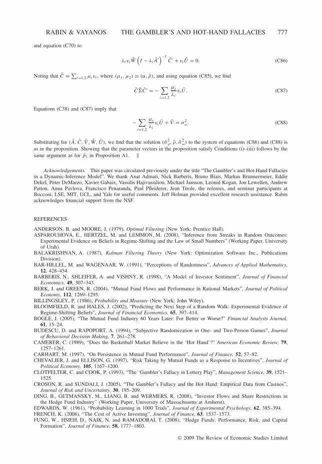
RABIN & VAYANOS THE GAMBLER’S AND HOT-HAND FALLACIES 777
and equation (C70) to
λiviW(I − λiA
′)−1
C ′ + viU = 0. (C86)
Noting that C = ∑i=1,2 μivi , where (μ1, μ2) ≡ (α, ρ), and using equation (C85), we find
C�C ′ = −∑i=1,2
μi
λi
viU . (C87)
Equations (C38) and (C87) imply that
−∑i=1,2
μi
λi
viU + V = σ 2ω. (C88)
Substituting for (A, C, V , W , U), we find that the solution (σ 2η, ρ, σ 2
ω) to the system of equations (C86) and (C88) isas in the proposition. Showing that the parameter vectors in the proposition satisfy Conditions (i)–(iii) follows by thesame argument as for p1 in Proposition A1. ‖
Acknowledgements. This paper was circulated previously under the title “The Gambler’s and Hot-Hand Fallaciesin a Dynamic-Inference Model”. We thank Anat Admati, Nick Barberis, Bruno Biais, Markus Brunnermeier, EddieDekel, Peter DeMarzo, Xavier Gabaix, Vassilis Hajivassiliou, Michael Jansson, Leonid Kogan, Jon Lewellen, AndrewPatton, Anna Pavlova, Francisco Penaranda, Paul Pfleiderer, Jean Tirole, the referees, and seminar participants atBocconi, LSE, MIT, UCL, and Yale for useful comments. Jeff Holman provided excellent research assistance. Rabinacknowledges financial support from the NSF.
REFERENCES
ANDERSON, B. and MOORE, J. (1979), Optimal Filtering (New York: Prentice Hall).ASPAROUHOVA, E., HERTZEL, M. and LEMMON, M. (2008), “Inference from Streaks in Random Outcomes:
Experimental Evidence on Beliefs in Regime-Shifting and the Law of Small Numbers” (Working Paper, Universityof Utah).
BALAKRISHNAN, A. (1987), Kalman Filtering Theory (New York: Optimization Software Inc., PublicationsDivision).
BAR-HILLEL, M. and WAGENAAR, W. (1991), “Perceptions of Randomness”, Advances of Applied Mathematics,12, 428–454.
BARBERIS, N., SHLEIFER, A. and VISHNY, R. (1998), “A Model of Investor Sentiment”, Journal of FinancialEconomics, 49, 307–343.
BERK, J. and GREEN, R. (2004), “Mutual Fund Flows and Performance in Rational Markets”, Journal of PoliticalEconomy, 112, 1269–1295.
BILLINGSLEY, P. (1986), Probability and Measure (New York: John Wiley).BLOOMFIELD, R. and HALES, J. (2002), “Predicting the Next Step of a Random Walk: Experimental Evidence of
Regime-Shifting Beliefs”, Journal of Financial Economics, 65, 397–414.BOGLE, J. (2005), “The Mutual Fund Industry 60 Years Later: For Better or Worse?” Financial Analysts Journal,
61, 15–24.BUDESCU, D. and RAPOPORT, A. (1994), “Subjective Randomization in One- and Two-Person Games”, Journal
of Behavioral Decision Making, 7, 261–278.CAMERER, C. (1989), “Does the Basketball Market Believe in the ‘Hot Hand’?” American Economic Review, 79,
1257–1261.CARHART, M. (1997), “On Persistence in Mutual Fund Performance”, Journal of Finance, 52, 57–82.CHEVALIER, J. and ELLISON, G. (1997), “Risk Taking by Mutual Funds as a Response to Incentives”, Journal of
Political Economy, 105, 1167–1200.CLOTFELTER, C. and COOK, P. (1993), “The ‘Gambler’s Fallacy in Lottery Play”, Management Science, 39, 1521–
1525.CROSON, R. and SUNDALI, J. (2005), “The Gambler’s Fallacy and the Hot Hand: Empirical Data from Casinos”,
Journal of Risk and Uncertainty, 30, 195–209.DING, B., GETMANSKY, M., LIANG, B. and WERMERS, R. (2008), “Investor Flows and Share Restrictions in
the Hedge Fund Industry” (Working Paper, University of Massachusetts at Amherst).EDWARDS, W. (1961), “Probability Learning in 1000 Trials”, Journal of Experimental Psychology, 62, 385–394.FRENCH, K. (2008), “The Cost of Active Investing”, Journal of Finance, 63, 1537–1573.FUNG, W., HSIEH, D., NAIK, N. and RAMADORAI, T. (2008), “Hedge Funds: Performance, Risk, and Capital
Formation”, Journal of Finance, 58, 1777–1803.
© 2009 The Review of Economic Studies Limited

778 REVIEW OF ECONOMIC STUDIES
GILOVICH, T., VALLONE, R. and TVERSKY, A. (1985), “The Hot Hand in Basketball: On the Misperception ofRandom Sequences”, Cognitive Psychology, 17, 295–314.
GOLD, E. and HESTER, G. (2008), “The Gambler’s Fallacy and the Coin’s Memory”, in J. Krueger (ed.) Rationalityand Social Responsibility: Essays in Honor of Robyn Mason Dawes (New York: Psychology Press).
GREENE, W. (2008), Econometric Analysis, 6th edn (New York: Prentice Hall).GRUBER, M. (1996), “Another Puzzle: The Growth in Actively Managed Mutual Funds”, Journal of Finance, 51,
783–810.McLEISH, D. (1975), “A Maximal Inequality and Dependent Strong Laws”, The Annals of Probability, 3, 829–839.METZGER, M. (1984), “Biases in Betting: An Application of Laboratory Findings”, Psychological Reports, 56,
883–888.RABIN, M. (2002), “Inference by Believers in the Law of Small Numbers”, Quarterly Journal of Economics, 117,
775–816.RAPOPORT, A. and BUDESCU, D. (1992), “Generation of Random Binary Series in Strictly Competitive Games”,
Journal of Experimental Psychology: General, 121, 352–364.RAPOPORT, A. and BUDESCU, D. (1997), “Randomization in Individual Choice Behavior”, Psychological Review,
104, 603–617.ROLL, R. (1992), “A Mean/Variance Analysis of Tracking Error”, Journal of Portfolio Management, 18, 15–24.SIRRI, E. and TUFANO, P. (1998), “Costly Search and Mutual Fund Flows”, Journal of Finance, 53, 1655–1694.TERRELL, D. (1994), “A Test of the Gambler’s Fallacy—Evidence from Pari-Mutuel Games”, Journal of Risk and
Uncertainty, 8, 309–317.TERRELL, D. (1998), “Biases in Assessments of Probabilities: New Evidence from Greyhound Races”, Journal of
Risk and Uncertainty, 17, 151–166.TERRELL, D. and FARMER A. (1996), “Optimal Betting and Efficiency in Parimutuel Betting Markets with
Information Costs”, The Economic Journal, 106, 846–868.TVERSKY, A. and GILOVICH T. (1989a), “The Cold Facts about the ‘Hot Hand’ in Basketball”, Chance, 2, 16–21.TVERSKY, A. and GILOVICH T. (1989b), “The Hot Hand: Statistical Reality or Cognitive Illusion?” Chance, 2,
31–34.
© 2009 The Review of Economic Studies Limited


![Gambler’s Ruin Bandit Problem · A. Gambler’s Ruin Problem If action F is removed from the GRBP, it becomes the Gambler’s Ruin Problem. In the model of Hunter et al. [10] of](https://img.pdfslide.net/doc/110x75/5f0c18f57e708231d433ba74/gambleras-ruin-bandit-problem-a-gambleras-ruin-problem-if-action-f-is-removed.jpg)