Understanding Address Usage in the Visible InternetUSC/ISI Technical Report ISI-TR-656, February 2009

Xue Cai John HeidemannUSC/Information Sciences Institute, {xuecai,johnh}@isi.edu

ABSTRACT

Although the Internet is widely used today, there are few

sound estimates of network demographics. Decentralized

network management means questions about Internet use

cannot be answered by a central authority, and firewalls and

sensitivity to probing means that active measurements must

be done carefully and validated against known data. Build-

ing on frequent ICMP probing of 1% of the Internet address

space, we develop a clustering algorithm to estimate how In-

ternet addresses are used. We show that adjacent addresses

often have similar characteristics and are used for similar

purposes (61% of addresses we probe are consistent blocks

of 64 neighbors or more). We then apply this block-level

clustering to provide data to explore several open questions

in how networks are managed. First, the nearing full allo-

cation of IPv4 addresses makes it increasingly important to

estimate the costs of better management of the IPv4 space

as a component of an IPv6 transition. We provide about

how effectively network addresses blocks appear to be used,

finding that a significant number of blocks are only lightly

used (about one-fifth of /24 blocks have most addresses in

use less than 10% of the time). Second, we provide new

measurements about dynamically managed address space,

showing nearly 40% of /24 blocks appear to be dynamically

allocated, and dynamic addressing is most widely used in

countries more recently to the Internet (more than 80% in

China, while less then 30% in the U.S.).

Categories and Subject Descriptors

C.2.1 [Computer-Communication Networks]: Net-work Architecture and Design—Network topology ; C.2.3[Computer-Communication Networks]: NetworkOperations—Network management

General Terms: Measurement

Keywords: Internet address allocation, survey, pat-tern analysis, clustering, classification, availability, volatil-ity

1. INTRODUCTION

Previous Internet topology studies focused on AS-and router-level topologies [3, 5, 7, 10, 21, 25, 26]. Whilethis work explored the core of the network, it provideslittle insight into the edge of the Internet and the useof the IPv4 address space. The transition to classlessrouting [9] in the mid-1990s has made the edge opaque.Only recently have researchers begun to study edge-hostbehavior using server logs [32], web search engines ontextual addresses [28], and ICMP probing [12].

Assumptions: In this paper we begin to explore thepotential of clustering of active probes to infer networkaddress usage. Our work makes three assumptions:

1. many active addresses will respond to probes,

2. contiguous addresses are often used similarly, and

3. patterns of probe responses suggest address usage.

While there are cases where these assumptions donot hold, we believe they apply to a large fraction ofthe Internet and so active probing can provide insightinto address usage. Recent work has shown that ac-tive probes detect the majority of addresses in use, con-firmed against large university and a random sample ofthe general Internet [12], supporting the first assump-tion.

We explore the rest assumptions in this paper. Ourassumption about contiguous use follows from the tra-ditional administrative practice of assigning blocks ofconsecutive addresses to minimize routing table sizesWhile there is no requirement that adjacent addressesbe used for the same purpose, we will show that theyoften used similarly (Section 5.1).

Finally, we assume that repeated active probing withICMP provides some information about how addressesare used. While ICMP provides only limited infor-mation (is the addresses responsive or not), repeatedprobing separates addresses in constant use from thoseused intermittently. We will show that these observa-tions correlate with servers or always-on-desktop com-puters and dynamically assigned address block (Sec-tions 4 and 6.1).

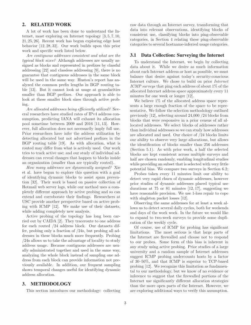
Figure 1 shows an example of what probing reveals,given one block of 256 addresses with prefix p1 where

1

Figure 1: A /24 block (prefix is anonymized to p1)where probing suggests seven different regions. Ad-dresses are on a Hilbert curve.

these assumptions apply1. Different shades indicate dif-ferent ping response patterns by each address (greenis availability and red is volatility, metrics we definelater in Section 3.2). This block clearly shows twodifferent patterns for seven address blocks. Manualexamination shows these regions correspond with webservers and dial-up addresses. Hostnames suggest thelower left quarter of the block (p1.0/26) bottom righteighth (p1.64/27), and middle left (p1.144/28) are pop-ulated mostly with web servers; except for a few un-occupied addresses, these regions are almost always upand so show as light colors. Hostnames in the dark re-gions, upper-right (p1.192/26), upper-left (p1.160/27),and middle-left (p1.96/27) suggest use for dial-up, andprobing shows they are only used infrequently and in-termittently.

Approach: From these assumptions we develop newalgorithms to identify blocks of addresses with consis-tent usage (Section 3). We start with Internet surveydata, where each address in around 24,000 /24 address

1Recall that IPv4 addresses are 32-bit numbers, usuallywritten in the form a.b.c.d, where each component is an8-bit portion of the whole address. Addresses are organizedin blocks (sometimes called subnetworks) that are sized topowers of two. Blocks have a common prefix, the lead-ing p bits of the address, written a.b.c.d/p. For example,128.125.7.0/24 indicates a /24 block with 256 addresses init of the form 128.125.7.x. We sometimes talk about blocksas p.0/24, where p represents the anonymized prefix.

blocks is pinged every 11 minutes for one week [12].From this dataset we derive several metrics about howeach address is used. We then use these statistics to au-tomatically identify blocks of consistent responsiveness.Ping responsiveness does not directly identify addressuse, so to get a better understanding of use we correlateour metrics with uses inferred from hostnames assignedto those addresses (Section 4).

Validation and Applications: Before applying thesealgorithms, we evaluate how often our assumptions hold.Our first question is therefore are adjacent addressesused consistently and can we discover them reasonablyaccurately? Before classless IP addressing [9] allocationstrategies were aligned with externally visible addressallocation, but since then there has been no way to eas-ily evaluate how addresses are used. We explore thesebasic questions in Sections 5.1 and 6.1.1.

A first application of this approach is to understandhow addresses are managed, beginning with what blocksizes are typical(Section 5.1). We find that 2,529,216addresses, or 61% of the probed address space, showconsistent responses in blocks of 64 to 256 adjacent ad-dresses (/26 to /24 blocks). And we observe that mostaddresses (around 55%) in the Internet are in /24 orbigger blocks.

A second application is to understand how effectivelyaddresses are used (Section 5.2). We find that a sig-nificant number of blocks are only lightly used (aboutone-fifth of /24s show less than 10% utilization). Thesequestions are of growing importance as the IPv4 ad-dress space nears full allocation; they help estimate thecosts of improving IPv4 efficiency as compared to IPv6transition.

Finally, we detect and quantify the use of dynamicaddress assignment (Section 5.3). Dynamic addressesare important for several reasons. Since they oftenrepresent poorly secured home computers, dynamic ad-dresses factor in to some spam detection algorithms [32].Identifying dynamic addresses is important to estimatethe number of computers that do connect to the In-ternet [12]. We observe that nearly 40% of /24 blocksappear to be dynamically allocated to computers, anddynamic addressing is much higher in countries mostrecent to the Internet (more than 80% in China, whileless then 30% in the U.S.).

The contribution of this paper is therefore to developnew approaches to classify Internet address usage and toapply those approaches to answer important questionsin network management. As with many prior studies ofthe Internet, our approach is based on limited informa-tion and we do not claim perfect accuracy. However, wesuggest the approach is promising and our preliminaryresults add important observations to what is currentlyknown.

2

2. RELATEDWORK

A lot of work has been done to understand the In-ternet, most exploring on Internet topology [3, 5, 7, 10,21, 25, 26]. Recent work has begun exploring edge hostbehavior [12, 28, 32]. Our work builds upon this priorwork and specific work listed below.

Are contiguous addresses consistent and what are thetypical block sizes? Although addresses are usually as-signed as blocks and represented in prefixes by classfuladdressing [22] and classless addressing [9], there is noguarantee that contiguous addresses in the same blockwill be used in the same way. Huston’s report has an-alyzed the common prefix lengths in BGP routing ta-ble [13]. But it cannot look at usage at granularitiessmaller than BGP prefixes. Our approach is able tolook at these smaller block sizes through active prob-ing.

Are allocated addresses being efficiently utilized? Sev-eral researchers have studied rates of IPv4 address con-sumption, predicting IANA will exhaust its allocationpool sometime between 2009 and 2016 [11, 13]. How-ever, full allocation does not necessarily imply full use.Prior researchers have infer the address utilization bydetecting allocated but not advertised prefixes in theBGP routing table [19]. As with allocation, what isrouted may differ from what is actively used. Our worktries to track active use; and our study of individual ad-dresses can reveal changes that happen to blocks insidean organization (smaller than are typically routed).

How many addresses are dynamically assigned? Xieet al. have begun to explore this question with a goalof identifying dynamic blocks to assist spam preven-tion [32]. Their work is based on passive collection ofHotmail web server logs, while our method uses a com-pletely different approach by active probing and so canextend and corroborate their findings. Researchers atUSC provide another perspective based on active prob-ing with ICMP [12]. We make use of their datasets,while adding completely new analysis.

Active probing of the topology has long been car-ried out by CAIDA [2]. They traceroute to one addressfor each routed /24 address block. Our datasets dif-fer, probing only a fraction of /24s, but probing all ad-dresses in these blocks much more frequently. Probing/24s allows us to take the advantage of locality to studyaddress usage. Because contiguous addresses are usu-ally administrated together and used in the same way,analyzing the whole block instead of sampling one ad-dress from each block can provide information not pre-viously available. In addition, our frequent samplingshows temporal changes useful for identifying dynamicaddress allocation.

3. METHODOLOGY

This section introduces our methodology: collecting

raw data through an Internet survey, transforming thatdata into relevant observations, identifying blocks ofconsistent use, classifying blocks into ping-observablecategories, in Section 4 relating these ping-observablecategories to several hostname-inferred usage categories.

3.1 Data Collection: Surveying the Internet

To understand the Internet, we begin by collectingdata about it. While we desire as much informationabout each Internet address or host as possible, we mustbalance that desire against today’s security-consciousInternet culture. We chose to build on prior InternetICMP surveys that ping each address of about 1% of theallocated Internet address space approximately every 11minutes for one week or longer [12].

We believe 1% of the allocated address space repre-sents a large enough fraction of the space to be repre-sentative. We follow the selection methodology outlinedpreviously [12], selecting around 24,000 /24 blocks fromblocks that were responsive in a prior census of all al-located addresses. We select blocks of addresses ratherthan individual addresses so we can study how addressesare allocated and used. Our choice of /24 blocks limitsour ability to observe very large allocations, but allowsthe identification of blocks smaller than 256 addresses(Section 5.1). As with prior work, a half the selectedblocks are kept consistent across multiple surveys andhalf are chosen randomly, enabling longitudinal studieswhile providing an subset that is selected with very littlepotential bias. We compare two surveys in Section 6.2;

Probes taken every 11 minutes limit our ability todetect very rapid churn of dynamic addresses, howeverprior studies of dynamic addresses placed typical usedurations at 75 or 81 minutes [12, 17], suggesting wehave reasonable precision. We use 1-loss repair to copewith singleton packet losses [12].

Observing the same addresses for at least a week al-lows us to detect several daily cycles, both for weekendsand days of the work week. In the future we would liketo expand to two-week surveys to provide some dupli-cation of the weekly cycle.

Of course, use of ICMP for probing has significantlimitations. The most serious is that large parts ofthe Internet are firewalled and choose not to respondto our probes. Some form of this bias is inherent inany study using active probing. Prior studies of a largeuniversity and a random sample of Internet addressessuggest ICMP probing undercounts hosts by a factorof 30–50%, and that ICMP is superior to TCP-basedprobing [12]. We recognize this limitation as fundamen-tal to our methodology, but we know of no evidence orinference to suggest that the firewalled portions of theInternet use significantly different allocation strategiesthan the more open parts of the Internet. However, weare exploring additional ways to verify this assumption.

3

Start Date /24 BlocksName (# days) probed respond. UseIT17ws [30] 2007-06-01 (10) 22,367 20,849 all

IT17wrs 2007-06-01 (10) 17,366 16,295 §4IT16ws [29] 2007-02-16 (6) 22,365 20,900 §6.2VUSC s [31] 2007-08-13 (9) 768 299 §6.1ISC-DS [15] 2007-01 hostnames §4RIR [23] 2007-06-13 block allocation §5

Table 1: Datasets used in this paper.

Table 1 shows the datasets we use in our paper. Weuse two ICMP surveys taken by USC [12]: IT17ws andIT16ws; IT17ws is the main dataset used in this paper,while we use IT16ws for validation in Section 6.2. Wecollected VUSC s at our enterprise in order to compareour inferences with network operators as discussed inSection 6.1. Finally, we use a domain name survey fromISC [15] for training in Section 4, comparing that withIT17wrs, an overlapping subset of IT17ws.

3.2 Data Representation: Observations of In-terest

Since one survey provides more than 5 billion obser-vations, it is essential to map that raw data into moremeaningful metrics that characterize address usage. Wecall this step data representation, and we define threemetrics: availability, the fraction of time an addressis responsive; volatility, a normalized representation ofhow many consecutive periods the address is responsive;and median-up, the median duration of all up periods.

To define these more formally, let

ri(a) = 1 or 0,∀i ∈ [1, Np]

be the positive or negative response of the ith of the Np

probes to address a after 1-loss repair [12]. If each probeis made at time ti, we can define the Nu up durations(Nu < Np) of a survey as

uj(a) = tej− tbj

, where

ri = 1,∀i ∈ [bj , ej ]

and r(bj)−1 = 0, r(ej)+1 = 0

∀j ∈ [1, Nu]

(each up duration is a consecutive run of positive probesfrom bj to ej , inclusive). We can now clarify that avail-ability, volatility, and median-up are given as:

A(a) =1

Np

(

Np∑

1

ri

)

V (a) = Nu/(Np/2)

U∗(a) = median(uj , ∀j ∈ [1, Nu])

Availability is normalized; it is the fraction of timesa host is reachable. Volatility is normalized by Np/2,the maximum number of states (alternating value each

time). For example, if Np = 16, and the responses ri ofaddress a are [1, 1, 0, 0, 1, 1, 1, 1, 0, 0, 0, 1, 1, 1, 1, 1], thenthere are three up periods (N − u = 3) of lengths 22,44, 55 minutes each. A(a) = 11/16 = 0.688, V (a) =3/(16/2) = 0.375 and U∗(a) = median(22, 44, 55) = 44minutes. (We also sometimes use un-normalized volatil-ity, V ∗(a) = Nu, simply the count of up periods.) Weconsidered normalizing median-up to measurement du-ration, but chose not to because such normalizationdistorts observations about hosts that are not nearlyalways present. Finally, we often omit the (a) when thesubject of the metric is clear.

While these metrics are not completely orthogonal,each has a purpose. Availability shows how effectivelyaddresses are used. High volatility indicates addressesthat are only intermittently used and often dynamicallyallocated. Median uptime suggests how long an addressis used.

These estimates assume the ri observations are cor-rect and represent a single host. Because we know ourdata collection omits firewalled hosts (Section 3.1), wegenerally ignore addresses that do not ever respond.More troubling are addresses that are used by multi-ple computers at different times—such addresses actu-ally represent multiple hosts. The purpose of dynam-ically allocated addresses is exactly to share one ad-dress with multiple computers, and we know dynamicassignment is common (see Section 5). If those hostsare used for different purposes (servers sometimes, andclients others), usage inference will be difficult and un-reliable. However, we believe that it is relatively un-common for a dynamic address to transition betweenclient and server use, since servers usually require sta-ble addresses. (There is some use of dynamic DNS toplace services on changing addresses. We believe suchuse is rare for most of the world but plan to explore thisissue in future work.)

3.3 Block Identification

We next use our observations about addresses to eval-uate block size. To do this identification we develop anew clustering algorithm.

We assume blocks are allocated in sizes that are pow-ers of two, so block identification is the process of find-ing a prefix where addresses in the block are used con-sistently. We find that some blocks are not used consis-tently, and different addresses show very different sta-bility. In our analysis we will keep dividing these mixed-use blocks until they are consistent, if necessary devolv-ing to a single address per block. Another challenge isthat many blocks have gaps where a few addresses areused differently, or are not responsive, perhaps becausethey are unused or firewalled. Our algorithm weighschoice of larger blocks with some inconsistencies againstsmaller but more homogeneous blocks.

4

We only consider blocks of sizes /24 or smaller be-cause current data collection method does not guar-antee blocks larger than /24s. (Exploration of largerblocks is an area of potential future work.)

3.3.1 Clustering background

Our goal with clustering of address responsiveness isto determine whatever blocks that appear to be usedconsistently. We therefore use partitional clustering,one of the two general approaches to clustering in thiswell developed field [16]. Partitional clustering placeseach element into exactly one cluster; we choose it overthe alternative, hierarchical clustering, which would placeitems into multiple, hierarchically nested clusters.

Jain describes partional clustering as: “Given n pat-terns in a d-dimensional metric space, determine a par-tition of the patterns into K groups, or clusters, suchthat the patterns in a cluster are more similar to eachother than to patterns in different clusters” [16]. Webuild on the basic approaches of clustering for our method:a pattern matrix, feature normalization, and use of anelbow criterion to select the best choice.

Although we follow traditional clustering theory, In-ternet addresses impose a unique restriction. Addressesare only grouped into blocks that are contiguous, sizesof powers of two, and aligned at multiples of the size.For these reasons, we cannot directly use traditional al-gorithms such as K-means, but instead use componentsof existing clustering approaches. The most radical dif-ference from traditional clustering is that addresses areonly clustered with some number of immediate neigh-bors, not with arbitrary other addresses. We thereforefind blocks of consecutive addresses by the definition ofour algorithm, however the size of blocks it finds de-pends on the consistency of how the addresses are used.

A Pattern Matrix defines the features over the spacebeing clustered. In our case, each address is defined byits three features (A, V, U∗), and the space is a numberof disjoint /24 blocks. Each /24 block has a 256×3 pat-tern matrix x∗

ij , where j enumerates the three features,and i enumerates each address in a /24 block. Fromour 24,000 /24 blocks we get 24,000 pattern matrices intotal.

Although our definitions of A and V are already nor-malized to the range [0, 1], their distribution may beskewed, and U∗ is not normalized. We therefore em-ploy feature normalization to give each features equalweight. We define the normalized feature vector xij ,given the mean and standard deviations mj and sj ofeach feature j:

xij =x∗

ij − µj

σj

where µj and σj are the mean and standard devi-ation. We use Euclidean distance between two com-ponents of the feature vector to measure dissimilarity

between two elements i and k over their features:

d(i, k) =

√

√

√

√

3∑

j=1

(xij − xkj)2

Many clustering algorithms, like K-means, requirethe number of clusters be chosen in advance. We can-not do that because clusters correspond to block size,a quantity we wish to discover. We also cannot simplyminimize variance, because variance is trivially mini-mized in the degenerate case where each cluster is asingleton address.

We therefore employ an elbow criterion, a commonrule of thumb to determine the number of clusters. Wesplit each cluster into two whenever splitting adds sig-nificant information, and we stop when we pass the “el-bow” of the curve and more clusters add little bene-fit. We measure information by the sum of variance ineach cluster across the population—homogeneous clus-ters will have low variance; splitting them adds no newinformation. Heterogeneous clusters have high variance,and splitting them into two more self-consistent piecesreduces the sum of variance, increasing the amount ofinformation.

3.3.2 Our Algorithm to Identify Block Sizes

Our algorithm follows the basic structure we outlineabove: we define a pattern matrix of addresses by fea-tures, normalize the features, then recursively search forclusters until reaching the elbow. We fill in the detailsnext.

The algorithm is a recursive function, BlockSizeId,taking an address-feature matrix 256 × (A, V, U∗) anda given prefix length P . Since the blocks in our surveyare disjoint, we iterate over each /24 block in our surveyseparately, beginning with P = 24.

BlockSizeId then computes the sum of intra-blockvariance for all possible prefix lengths p(P ≤ p ≤ 32)and selects smallest prefix length pelbow where longerprefixes show minimal change. We define vsump as sumof intra-block variance of sub-blocks with prefix lengthp:

np = 2p−P , sp = 232−p, µbj =

∑bsp

i=(b−1)sp+1 xij

sp

vb =3

∑

j=1

bsp∑

i=(b−1)sp+1

(xij − µbj)2, 1 ≤ b ≤ np

vsump =

np∑

b=1

vb, P ≤ p ≤ 32

where np is the number of sub-blocks with prefixlength p, sp is the size of sub-blocks (number of ad-dresses) with prefix length p. For example, if P = 24and p = 27, then np = 8 and sp = 32. mbj is the mean

5

value of the jth feature of addresses in the bth sub-block.vb is the intra-block variance of the bth sub-block. Inthis example, it would be the intra-block variance of thebth /27 sub-block.

We define minimal change in the elbow algorithmwith an empirically selected constant threshold, ǫ. Weselect pelbow as some p such that vsump+1−vsump < ǫ.If pelbow = P , then no division of this block reducesvariance significantly and we terminate our recursivealgorithm, declaring P the consistent block size. If thiscase does not hold, we have determined there are splitsof the block that appear to be more consistent. We thensplit the block in half and recurse, calling BlockSizeIdwith the next longer prefix P = p + 1 on each half ofthe data. In principle, a block could be split repeatedlyuntil it is composed on a single address and the algo-rithm terminates with zero variance. In practice, inSection 5.1 we show that the majority of the Internetaddresses fall into larger blocks of consistent use.

3.3.3 A Block Identification Example

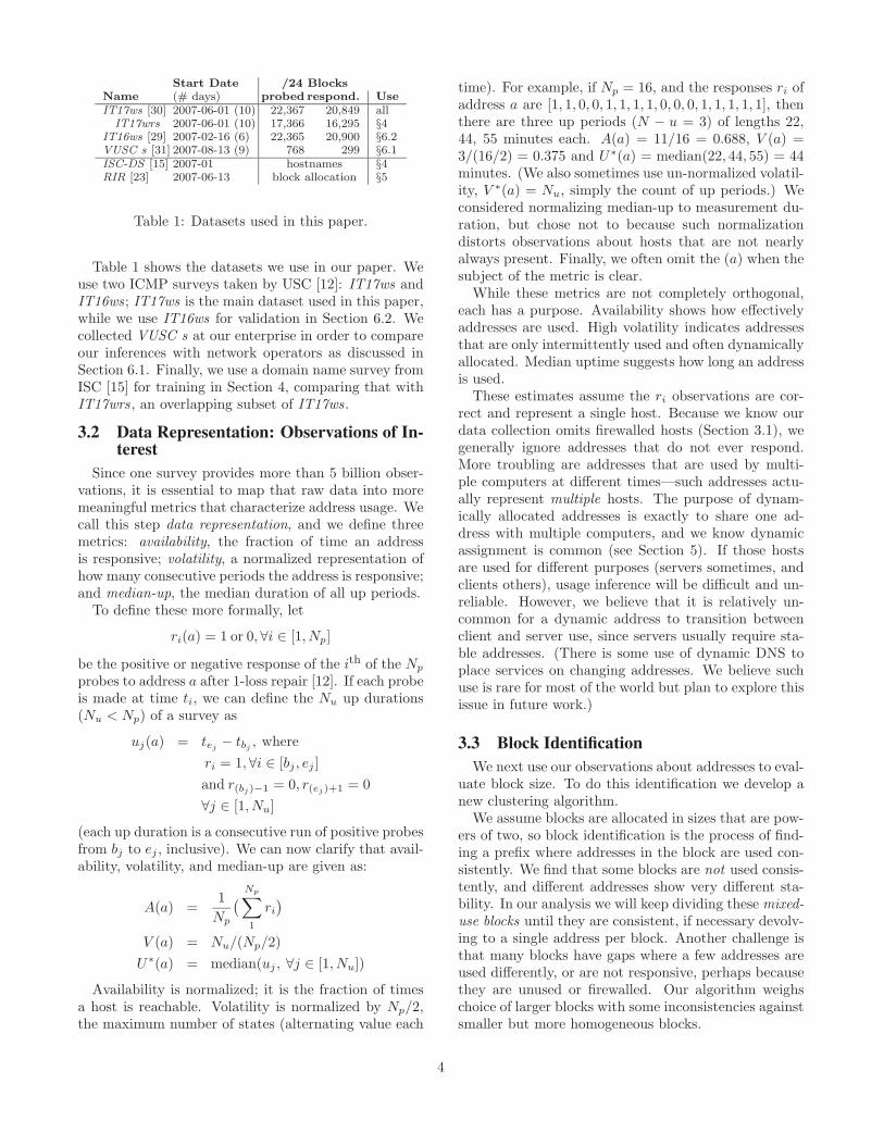
To illustrate BlockSizeId we next show analysis of anexample /24 block taken from the Internet. Figure 2shows the whole p2.0/24 surveyed block and the processof identifying the 4 consistently used blocks inside of /24subnetwork. To a human observer, common patterns inthe block are the /25 block on the left (red, indicatinglarge volatility), a /27 block on the top right (dark red,indicating low availability and moderate volatility), asecond /27 block on the bottom right (dark red), andthe third /27 block on the bottom right (green, indi-cating high availability and low volatility). Unlike Fig-ure 1, this block does not have reverse DNS entries andso we cannot confirm these assumptions with hostnamesas the method shown in Section 4.

The graph immediately under the address plot in Fig-ure 2 the first pass of BlockSizeId for the feature ma-trix for p2.0/24 and P = 24. In the graph, the y-axisshows variance for division of the block into each pos-sible power-of-two smaller size. Here pelbow = 25 andpelbow > P , so we recurse on p2.0/25 and p2.128/25with P = 25.

The second row of two graphs shows these two re-cursive invocations, p2.0/25 on the left and p2.128/25on the right. First, considering p2.128/25 the graphon the right shows a consistent variance regardless ofsubdivision, and pelbow = P = 25. This prefix appearsto be consistently used and this branch terminates suc-cessfully. Second, for p2.0/25 (the graph on the left),a subdivision reduces variance and so we recurse againwith P = 26.

The algorithm recurses until either pelbow = P orP = 32. In this example, the initial /24 block is dividedinto p2.0/27, p2.32/27, p2.64/27, and p2.128/25.

3.4 Ping-Observable Block Classification

0 0.2 0.4 0.6 0.8

1 1.2

/24 /25 /26 /27 /28 /29 /30 /31 /32

Variance

Prefix Length

p2.0/24

0 0.2 0.4 0.6 0.8

1 1.2

/25 /26 /27 /28 /29 /30 /31 /32

Variance

Prefix Length

p2.0/25

0 0.2 0.4 0.6 0.8

1 1.2

/25 /26 /27 /28 /29 /30 /31 /32

Variance

Prefix Length

( p2.128/25 )

0 0.2 0.4 0.6 0.8

1 1.2

/26 /27 /28 /29 /30 /31 /32

Variance

Prefix Length

p2.0/26

0 0.2 0.4 0.6 0.8

1 1.2

/26 /27 /28 /29 /30 /31 /32V

ariance

Prefix Length

p2.64/26

0 0.2 0.4 0.6 0.8

1 1.2

/27 /28 /29 /30 /31 /32

Variance

Prefix Length

( p2.0/27 )

0 0.2 0.4 0.6 0.8

1 1.2

/27 /28 /29 /30 /31 /32

Variance

Prefix Length

( p2.32/27 )

0 0.2 0.4 0.6 0.8

1 1.2

/27 /28 /29 /30 /31 /32V

ariance

Prefix Length

( p2.64/27 )

Figure 2: An example of BlockSizeId with thresholdǫ = 2.0. A plot of the addresses is shown (top), whileeach row of graphs shows the variance at each recur-sion. Graphs of the four selected blocks are labeledwith (parentheses).

We can now take remote measurements, convert theminto observations, and use them to identify blocks ofconsistent neighboring addresses. We generalize our ob-servations on addresses into observations about a blockb by taking the median value of each observation:

(A(b), V (b), U∗(b)) = median(A(a), v(a), U∗(a)) ∀a ∈ b

We then classify these blocks into five ping-observablecategories, using (A(b), V (b), U∗(b)). We use four thresh-olds, αH = 0.95, indicating high availability, αL =

6

0.10, indicating low availability, β = 0.0016, for lowvolatility, and γ = 6 hours, corresponding to a rel-atively long uptime. The specific thresholds we giveare somewhat arbitrary, but were selected to providereasonably good correspondence between these ping-observable categories and the hostname-inferred usagecategories described next in Section 4. We examine sen-sitivity to our choices in Section 6.2.

Always-stable : highly available and stable.

(A ≥ αH) ∧ (V ≤ β)

Sometimes-stable : changing more often than always-stable, but frequently up continuously for long pe-riods (high U∗).

(U∗ ≥ γ) ∧ (A ≥ αL) ∧ (A < αH ∨ V > β)

Intermittent : individual addresses are up for shortperiods (low U∗):

(U∗ < γ) ∧ (A ≥ αL) ∧ (A < αH ∨ V > β)

Underutilized block : although addresses are occa-sionally used, they show low A values.

A < αL

Unclassifiable : we decline to classify blocks with fewactive responders. Currently we consider any blockwhere fewer than 20% of addresses responding asunclassifiable.

We selected these categories to split the majority ofthe (A, V, U∗) space.

Appendix A shows how these terms divide the space.

4. TRAININGANDHOSTNAME-INFERRED

USAGE CATEGORIZATION

Our methodology takes data about use of public ad-dresses and produces five ping-observable categories.We would like to relate those categories to terms thatare more meaningful to network operators, and to findwhat root causes correspond to and potentially causeblocks to be intermittent or underutilized.

Determining the operational characteristics of a net-work is quite challenging, however. In some cases we areable to discuss network policy with the operations staffto confirm our assumptions; we will use this approachto validate our conclusions against a large campus net-work in Section 6. However, such observations may bebiased by the policies of a single institution. We wouldlike to also draw data from the Internet at large, butit is infeasible to contact operations for large parts ofthe network. While tools such as nmap [18] can extract

ping survey 4,445,696 (100%)

ping responders 1,675,121 (37.7%)

ping survey w/ hostnames

2,197,373 (49.4%)

ping responders w/ hostnames

1,049,842 (23.6%)

ping responders

w/ hostnames

w/ keywords

573,494 (12.9%)

Figure 3: Our Investigation Targets: IP addresses everresponded in IT17wrs and have meaningful hostnames(with keywords). It is the middle part with 573,494addresses in this figure.

significant information from a network through sophis-ticated active probing, their use is easy confused withhostile network activity by many network operations.2

Hostnames are a source of data that provides someinformation about how public computers are used—many hostnames contain keywords such as “www”, “dy-namic”, or “dsl”. Wide hostnames collection is also fea-sible: many Internet hosts suggest reverse DNS lookup [20],reverse lookup occurs commonly as part of normal op-eration and so is unlikely to be seen as hostile. TheInternet Systems Consortium has collected full tablesof reverse DNS regularly since 1994 [15] and makes itavailable for a nominal fee.

We next describe how we map hostnames to 15 hostname-inferred usage categories, and how this data correspondsto our five ping-observable categories.

While one might study the Internet using hostnamedata alone, without ping data, we believe the informa-tion complements each other. About half addresses thatare used lack reverse hostnames, and about 49% of host-names lack meaningful keywords, and reverse namesmay not represent the computer’s true use (for hostswith multiple names, where often the reverse name isautomatically assigned) so we think hostnames aloneare not sufficient.

4.1 Hostname-inferred Usage Categories

Although hostnames are not perfect, we believe theyprovide a useful dataset to compare against our ping-observable categories. We use ISC survey 17 [14], takenslightly before the ping survey used for our primaryanalysis [30].

2Widescale nmap use would place us in contact with addi-tional operations staff, but perhaps not on ideal terms.

7

group category keywords countallocation static static 28,137

dynamic dynamic, dyn 105,882dhcp dhcp 14,290pool pool, pond 66,009ppp ppp 44,729

access link dial dial, modem 80,090dsl dsl 208,682cable cable 29,761wireless wireless, wifi 910ded ded, dedicated 733

consumer biz business, biz 12,999res res, resident 25,847client client 9,994

server server server, srv, svr, mx,mail, smtp, www, ns, ftp

12,568

router router, rtr, rt, gateway,gw

2,850

Table 2: Categories of hostname-derived usage.

0

50000

100000

150000

200000

250000

static dynamic dhcp pool ppp dial dsl cable wireless ded biz res client server router

Nu

mb

er

of

Ho

sts

Hostname-inferred Usage Categories

unknownsingletondynamic

static

Figure 4: Numbers of hostname-inferred usage cate-gories, with colors indicating those that also have al-location types.

Figure 3 shows the overlap of these datasets. showsour investigation targets. We begin with the 4.4M IPaddresses probed the ping survey Nearly half of these(2.2M) have hostnames in the ISC reverse DNS survey.Of the 1.6M ping addresses that respond, we considerthe 1.0M addresses that also have hostnames. We thenfocus on the 573,494 of those that have identifiable key-words in their hostname (12.9% of all addresses in theping survey).

We follow recommendations that were proposed asstandard naming conventions for Internet hosts [27] andthat occur in 2000 or more hosts in our dataset. Al-though these were neither approved by the IETF, norwould the be mandatory even if approved, these termsdo appear in about one-quarter of reverse hostnames.From their recommendations we define 15 hostname-inferred usage categories as shown in Table 2.

Figure 4 shows the count of hostnames in each cat-egory. The sum exceeds 573k because these categoriespartially overlap, and a single hostname may be in mul-tiple categories. For example, some providers label DSLaddresses with both DSL and static or dynamic. We seethat access links keywords (DSL, dial, etc.) are verycommon, occurring in 51% of hostnames, and alloca-tion types (static, dynamic, etc.) occur in about 22%of hostnames in ping survey w/ hostnames.

0

20

40

60

80

100

0 0.1 0.2 0.3 0.4 0.5 0.6 0.7 0.8 0.9 1

Cu

mu

lative

Dis

trib

utio

n o

f H

osts

(%

)

Availability

staticdynamic

dhcppoolpppdialdsl

cablewireless

dedbizres

clientserverrouter

Figure 5: CDF of address availability (A) by hostname-inferred categories in IT17ws.

To provide some understanding the number of host-names with multiple keywords, we subdivide each cate-gory by those that also contain static, dynamic, or anyother additional keyword. Several groups types oftenhave an additional indication of allocation type: while10% of dsl are labeled dynamic (1.2% static), 50% ofbiz are labeled static. These secondary attributes re-veal some technology trends: the ratio of dial also withstatic or dynamic types is around 1:17, while for DSLit is 1:8 suggesting increased use of static addresses inalways-on DSL lines. For cable the ratio is 1:1, butthe fraction of cables with an additional type is smallenough that drawing conclusions may be risky.

4.2 Relating Hostname-Inferred toPing-Observable Categories

Our goal in evaluating hostnames is to use them tounderstand and train our ping-observable categories.We next compare the two to see when of our observa-tions (A, V, U∗) are correlated with hostname-inferredusage categories.

Figures 5, 6, and 7 show cumulative distribution func-tions of each observation against each hostname-inferredtype. This data will prove essential to understand theroot network causes of address underutilization and lo-cations of dynamic addresses; we therefore defer a de-tailed discussion of this data to Sections 5.2 and 5.3.

Taken together, though, these graphs support thethird assumption of our paper, that patterns of probe

responses can suggest address usage. This asser-tion is supported because hostname-inferred categories(our approximation of usage) show fairly distinct dis-tributions, particularly in availability (Figure 5) andmedian-uptime (Figure 7). As a specific example, Fig-ure 5 shows that availability of more than 50% dial ad-dresses is smaller than 0.1, while the A of more than80% server addresses is larger than 0.95.

While the bulk of dial and server addresses are quite

8

0

20

40

60

80

100

0.003 0.008 0.016 0.039 0.156 1

2 5 25 639 1 10 100C

um

ula

tive

Dis

trib

utio

n o

f H

osts

(%

)

Volatility

Volatility*

staticdynamic

dhcppoolpppdialdsl

cablewireless

dedbizres

clientserverrouter

Figure 6: CDF of address volatility (V ) by hostname-inferred category in IT17ws. Uptime counts (V ∗) isshown along the top x-axis.

0

20

40

60

80

100

6 0 20 40 60 80 100 120 140 160 180 200 220

Cu

mu

lative

Dis

trib

utio

n o

f H

osts

(%

)

Median Uptime (Hour)

staticdynamic

dhcppoolpppdialdsl

cablewireless

dedbizres

clientserverrouter

Figure 7: CDF of address median-up duration (U∗) byhostname-inferred category in IT17ws.

different, there are a few dial addresses with reasonablylarge A (5.4% have A > 0.5), and a moderate num-ber of servers have poor availability (about 10% haveA < 0.15). We conclude that, while ping-observablemetrics are reasonable predictors of usage, they are farfrom exact, and any estimates will have fairly large errorbounds. Perhaps this result is in keeping with previousobservations about the great variability of the Inter-net [8].

Finally, we use the observations in these CDFs to setour thresholds for ping-observable classes (Section 3.4).The sharp knees at A = 0.1 in Figure 5 suggest αL =0.1. Based on V in Figure 6, we select β = 0.0016to separate most servers and stable uses from less sta-ble. Finally, the sharp knee at around U∗ = 6 hoursin Figure 7 suggests this value for γ, This cutoff helpsseparate addresses which are not always-stable and notunderutilized to two categories: sometimes-stable andintermittent.

Based on these thresholds, Figure 8 and Table 3 mapthe 15 hostname-inferred usage categories to the ping-

0

200

400

600

800

1000

1200

1400

static dynamic dhcp pool ppp dial dsl cable wireless ded biz res client server router

Nu

mb

er

of

/24

Blo

cks

Hostname-inferred Usage Categories

[Ping-observable Categories]

unclassifiableunderutilized

intermittentsometimes-stable

always-stable

Figure 8: Relationship of ping-observed categories tohostname-inferred categories in IT17ws.

ping-observablecategory

hostname-inferred usagecategory

always-stable router, server, (static), ded,(biz), (dhcp), (res)

sometimes-stable res, static, biz, dhcp, (server),ded, (client), (cable), (dsl),(router), (ppp)

intermittent cable, dynamic, dsl, (wireless),(dial), (ppp), (dhcp)

underutilized pool, wireless, ppp, dial, client,(dynamic), (ded), (dsl)

Table 3: The mapping from the 15 hostname-inferred usage categories to 4 ping-observable cat-egories. hostname-inferred usage category without(parentheses) is dominate.

observable categories (Section 3.4).

5. APPLICATIONS

Having laid the groundwork for address analysis, wenext use the data to explore several questions in networkmanagement: what are typical sizes of consistently usedInternet address blocks? How effectively are they beingused? And how prominent is dynamic addressing?

To assist in answering some of these questions wecompare our observations with allocation data from theregional Internet registries (RIRs) [1]. This RIR dataincludes the time and country to which each addressblock is assigned. Although not completely authorita-tive, this data is the best publicly available estimate ofaddress delegation of which we are aware. We collecteddata from each of the RIRs, selecting data dated June13, 2007, to closely match our survey data.

5.1 Block Sizes

We begin by considering block sizes. Figure 9 andTable 4 show our data.

First, we observe that most addresses in the Inter-net are in /24 blocks. In fact, even though there moreopportunities for small blocks, we find more /24 blocksthan blocks of size /25 through /29. Since our data col-lection only probes consecutive runs of 256 addresses,this prevalence suggests we may need to probe largerconsecutive areas to understand if even larger blocksare common but not seen in our survey.

9

0

500000

1e+06

1.5e+06

2e+06

2.5e+06

3e+06

3.5e+06

/24 /25 /26 /27 /28 /29 /30 /31 /32

Nu

mb

er

of

Ad

dre

sse

s

Block Prefix Length

[Ping-observable Categories]

unclassifiableunderutilized

intermittentsometimes-stable

always-stable

Figure 9: Number of addresses in each block size andping-observable categories in IT17ws.

There are a very large number of the smallest blocks,with about as many /29s as /24s, and roughly twiceas many /30s as /29s, and /31s as /30s. These resultsmay be artifacts of our block discovery algorithm: it isstatistically easier for an address to be consistent witha very few neighbors in a small block than with 128neighbors in a /25. Finally, we can re-examine the sec-ond assumption underlying our work: are contiguousaddresses often used similarly? If we define consistentusage as just the largest three block sizes (/24 through/26) that we successfully identify, we find 2,529,216 ad-dresses are used consistently, or 44% of the probed ad-dress space.

While clearly defined, this percentage does not accu-rately present how much of the Internet is consistentlyused. Some of the probed address space is unclassifi-able (with consistent usage but fewer than 20% of ad-dresses responding), or completely non-responsive. Wecannot say anything about blocks that fail to respondat all. The status of unclassifiable blocks is uncertain,but a conservative position is to declare them inconsis-tent. A more representative evaluation of the Internetis therefore compare how much is definitely used consis-tently (2.5M addresses in large blocks) against that iseffectively inconsistent (the 506,178 addresses in smallblocks) and the possibly inconsistent (the 1,087,472 ad-dresses in unclassifiable blocks). This computation sug-gests that a lower bound of 61% of the responsive In-ternet is used consistently, We believe this supports oursecond assumption: the majority of contiguous ad-

dresses are used consistently.

5.2 Address Utilization

Having characterized block sizes, we next evaluatehow efficiently addresses are used. If IPv4 addressesare used inefficiently that represents an opportunity for

improvement. However, greater efficiency comes withgreater management cost; that cost must be weighedagainst simpler solutions such as IPv6.

5.2.1 Quantifying underutilization and possible causes

The underutilized ping-observable category is definedas a sequence of addresses that are used less than 10%of the time (Section 3.4). While one can imagine somecircumstances where a public IP address that is usedvery infrequently might make sense (for example, per-haps a DTN satellite only infrequently in view [6]), largeblocks of such addresses appear to represent a poor useof a public IP address. Moreover, these underutilizedblocks are not simply public address space hidden be-hind a firewall (a common management practice to sim-plify routing), but large blocks where each address isvisible, but only very infrequently.

The underutilized column of Table 4 shows that theseblocks are quite common, accounting for 17–23% ofblocks of each size, Although not shown in the table,the mean availability of addresses in /24 underutilizedblocks is only 3.2% of our 10-day observation (IT17ws).Manual examination of addresses show the mean num-ber of up periods is less than 5 (V ∗(b) = 4.6), typicallyfor around 1 hour (U∗(b)).

To understand why there are blocks of underutilizedaddresses we turn to our hostname–ping analysis fromSection 4.2. Figure 8 shows that underutilization corre-sponds with several hostname-inferred usage categories,including large fractions of categories dial and pool, andlarge absolute numbers of ppp, dsl and dynamic. Ouranalysis of hostname categories supports this observa-tion, where dial has low availability and median-uptime(Figures 5 and 7 and high volatility (Figure 6).

We hypothesize that this low utilization is tied todial-up technology itself. Dial-up lines are often sharedwith voice communication, encouraging short, intermit-tent use. Yet dial-up POPs must be provisioned tohandle peak loads. A secondary factor may be trendsshifting customers from dial-up to higher speed connec-tions. Perhaps old dial-up provisioned blocks are simplyin lower demand than previously. Finally, while dial-uputilization is low, we cannot tell how many users eachdial-up address serves. Perhaps address reuse is highenough to make these apparently underprovisioned ad-dresses a bargain relative to supporting the same num-ber of users with always-on connections.

Reversing the question, we can ask which addressblocks are well utilized? Figure 8 shows that the cate-gories of static, cable, biz, res, server, router have veryfew underutilized addresses. Static addresses are usu-ally assigned to fixed-location desktops or businesses,and these computers tend to maintain Internet connec-tion and occupy their address for a fairly long time.In addition, static addresses are often billed at a flat

10

blocks addressessize sometimes- classifiable unclassifiable [100%]

pfx addrs always-stable stable intermittent underutilized (100%)/24 256 1,603(18%) 2,517(29%) 2,673(30%) 1,994(23%) 8,787* 3,411 [27%] 12,198 3,122,688/25 128 323(23%) 523(38%) 295(21%) 237(17%) 1,378* 920 [40%] 2,298 294,144/26 64 346(21%) 617(38%) 378(23%) 274(17%) 1,615* 787 [33%] 2,402 153,728/27 32 432(20%) 855(40%) 506(23%) 361(16%) 2,154† 872 [29%] 3,026 96,832/28 16 759(20%) 1,301(34%) 993(46%) 734(19%) 3,787† 1,139 [23%] 4,926 78,816/29 8 2,077(21%) 3,190(32%) 2,355(24%) 2,227(23%) 9,849† 0 9,849 78,792/30 4 3,312(19%) 5,656(33%) 4,679(27%) 3,707(21%) 17,354† 0 17,354 69,416/31 2 4,195(16%) 9,867(37%) 7,864(30%) 4,566(17%) 26,492† 0 26,492 52,984/32 1 52,646(30%) 42,847(24%) 43,266(25%) 36,707(21%) 175,466† 0 175,466entire IT17ws dataset: (1,603,086 addrs. in non-responsive blocks) + (4,122,866 in responsive blocks) 22,367 5,725,952

Table 4: Number of blocks of each size in IT17ws. Unclassifiable percentages relative to all blocks; other percentagesrelative to classifiable blocks.

0

20

40

60

80

100

unknown 1985 1990 1995 2000 2005

Perc

enta

ge(%

)

Year

underutilizedintermittent

sometimes-stablealways-stable

Figure 10: Trend of ping-observable category change inIT17ws /24 blocks

rate per month, while dynamic addresses may incur atime-metered charge.

5.2.2 Locations and trends of underutilization

Evaluating underutilization by country may highlightpolicy differences by regional registries or ISPs. Aftermerging our data with RIR data, Table 5 shows utiliza-tion by country. We see that the United Kingdom andJapan have the largest fraction of underutilized blocks,40–60%, suggesting potential local policy differences.We expected a large number of underutilized blocks inthe U.S. because of wide deployment of dial-up. Whilethe U.S. has the largest absolute number of underuti-lized blocks, its fraction is relatively low.

Table 6 shows that the fraction of underutilized blocksis fairly consistent by across all five RIRs, suggestingdifferences are likely due to country, not RIR policies.

Finally, the lower right graph in Figure 10 showswhen underutilized blocks were allocated. The fractionof underutilized blocks by age seems fairly evenly dis-tributed, except for peaks in very early allocations (1984and unknown), where more than 60% of the blocks as-signed are underutilized. Since that pre-dates widespreaddialup, we do not have an immediate explanation forthis peak.

5.3 Dynamic IP Addressing

DHCP’s automatic address assignment [4] supportscentral assignment of IP addresses dynamically, requir-ing addresses only when users connect to the Internet.Although DHCP can be used to assign the same ad-dress to an always-up host, here we are interested inrelatively assignments that change frequently, possiblyfor hosts that are only intermittently connected.

Dynamic assignment assignment of addresses allowsISPs to multiplex many users over fewer addresses. Dy-namic addressing also provides ISPs the business op-portunity of offering static addresses as a higher-pricedservice, and potentially makes it more difficult for usersto operate bandwidth-consuming services.

To users, dynamic addressing has been promoted asa security advantage, on the theory that a compromisedcomputer is more difficult to contact if its IP addresschanges. They impede users from some Internet activi-ties, such as running services or accepting unsolicitedinbound connections (for example, for incoming SIPcalls). Wide use of dynamic addressing has promotedwork-arounds to these problems such as STUN [24].

Dynamic addresses also complicate some network ser-vices, such reputation systems, and are correlated withspam sources. These reasons suggest a better under-standing of dynamic addressing is important, and haveprompted recent study [12, 28, 32]. We next show thatour approach can identify dynamic addressees and sug-gest causes and trends that have been previously invis-ible.

5.4 Quantifying dynamic addressing

We believe that the intermittent and underutilizedping-observable categories correspond with the short-term dynamically assigned addresses we are interestedin. This statement is supported by hostname data,where Figure 8 shows that intermittent blocks are promi-nent in hostnames that include dynamic, pool, ppp,dial, dsl, and cable, all of which often use short- ormoderate-term dynamic addressing, and underutilizedblocks are common to dynamic, pool, ppp, dial, anddsl.

11

blockssometimes- classifiable unclassifiable [100%]

code country always-stable stable intermittent underutilized (100%)US US 673(27%) 1,106(45%)* 231(9.3%) 472(19%) 2,482 1,383 [36%] 3,865CN China 39(4.1%) 117(12%) 615(65%)* 171(18%) 942 132 [12%] 1,074JP Japan 383(48%)* 50(6.2%) 18(2.2%) 350(44%)* 801 288 [26%] 1,089DE Germany 65(10%) 125(20%) 388(61%)* 62(9.7%) 640 56 [8.0%] 696KR Korea 21(4.6%) 131(29%) 237(52%)* 68(15%) 457 142 [24%] 599FR France 18(4.1%) 227(52%)* 167(38%) 28(6.4%) 440 58 [12%] 498GB UK 39(13%) 37(12%) 52(17%) 179(58%)* 307 180 [37%] 487BR Brazil 7(3.9%) 35(19%) 86(48%)* 52(29%) 180 58 [24%] 238

all others 358(14%) 689(27%) 879(35%) 612(24%) 2,538 1,114 [31%] 3,652/24 blocks in entire IT17ws dataset: 8,787 3,411 [27%] 12,198

Table 5: The distribution of /24 blocks in ping-observable categories of 10 countries.

blockssometimes- classifiable unclassifiable [100%]

registry always-stable stable intermittent underutilized (100%)RIPENCC 408(14%) 798(27%) 1,084(37%)* 661(22%) 2,951 990 [25%] 3,941

APNIC 473(18%) 422(16%) 1,091(40%)* 716(27%) 2,702 795 [23%] 3,497ARIN 706(27%) 1,185(45%)* 258(9.7%) 512(19%) 2,661 1,481 [36%] 4,142

LACNIC 13(3.2%) 94(23%) 218(53%)* 86(21%) 411 120 [23%] 531AFRINIC 3(4.9%) 18(30%) 21(34%)* 19(31%) 61 19 [24%] 80/24 blocks in entire IT17ws dataset: 8,787 3,411 [27%] 12,198

Table 6: The distribution of /24 blocks in ping-observable categories of 5 regional registries.

Table 4 shows that there are many dynamic addresses:40–50% of classifiable blocks (depending on block size)appear to be dynamic. Even with wide deploymentof always-on connectivity, nearly half of Internet ad-dresses are used for short periods of time. For inter-mittent blocks, the mean availability is just under 30%,with nine use periods over the week and a the mean U∗

around 2.5 hours.

5.5 Locations and trends for dynamic address-ing

Analysis by country can suggest how political or cul-tural factors affect dynamic addressing. Table 5 showsthat nearly two-thirds of Chinese blocks are intermit-tent, with Germany, Korean, and Brazil all nearly halfor more. Several factors are potential causes for thisuse.

China has a very large population and is a relativelatecomer to the Internet; from the beginning of com-mercial deployment in China ISPs have planned to makebest use of relatively few IPv4 addresses per potentialuser. They have therefore promoted dynamic use to im-prove address utilization. An interesting direction forfuture work would be to evaluate how effective theirutilization is. Unfortunately we only know address re-sponsiveness, not the number of actual computers usersper address needed to answer this question.

Time-metered billing is another reason for intermit-tent use. Parts of China and Germany employ meteredbilling, encouraging intermittent use even with broad-band. Other potential reasons for intermittent use in-clude turning off a router to conserve energy, or carryingover habits learned from dial-up use to broadband, and

potentially continued use of dial-up connections sharedwith voice communication.

Evaluation of usage by regional registry in Table 6presents even larger differences in use. We see that in-termittent blocks are very prominent under APNIC andLACNIC (40–53%), five times more common than forARIN in North America (9%). We believe these dif-ferences stem largely from policies of the countries theRIRs serve, not the RIRs themselves. We discussedChinese practice above; several Latin American coun-tries have limited choice in ISPs, with national providersadopting pricing schemes that strongly favor dynamicaddress assignment even for business use. We specu-late that the large number of sometimes-stable blocks inARIN is because of long DHCP lease times and always-on use by home users, enabled by relatively plentifulnumbers of IPv4 addresses per user.

Finally we turn to trends in dynamic addressing. Thelower left portion of Figure 10 shows intermittent blocksare increasingly likely in new address allocations. Thisobservation is consistent with a growing recognition ofeventual full allocation of the IPv4 address space andefforts to manage addresses in countries newer to theInternet. The rise in intermittent blocks matches a cor-responding fall in always-stable blocks (top left, Fig-ure 10). In addition to growing demand for dynamicaddressing, this trend suggests most new addresses areadded to provide service for home users, intermittently.While the absolute numbers of always-stable businessesand servers grows, its fraction of all addresses is shrink-ing.

6. VALIDATION

12

0

5000

10000

15000

20000

25000

30000

35000

40000

/24 /25 /26 /27 /28 /29 /30 /31 /32

Nu

mb

er

of

Ad

dre

sse

s

Block Prefix Length

[Ping-observable Categories]

unclassifiableunderutilized

intermittentsometimes-stable

always-stable

Figure 11: Number of addresses in each block size andping-observable categories in ITUSC s.

The conclusions of this paper are based on the threeassumptions we listed in the introduction: addressesrespond to probes, adjacent addresses have similar use,and probes suggest use. Validation of the first assump-tion is the subject of prior work [12]; space prohibitsrevisiting that work here.

We have already presented data on the two final as-sumptions, showing that the majority of contiguous ad-dresses are used consistently (Section 5.1) and proberesponses can suggest use (Section 4.2). These conclu-sions are based on data taken from one survey IT17wsfrom the general Internet. While not biased, we cannotcompare these results to the true network configurationthat is distributed across thousands of enterprises. Wenext present two additional studies to further validatethese assumptions. First we evaluate data taken fromUSC, a smaller and potentially biased dataset, but onewhere we have ground truth from the network oper-ations staff. We then compare compare our Internet-wide results with a second dataset, IT16ws, to verifyour conclusions do not reflect something unusual in asingle time or set of addresses.

6.1 Validation within USC

We first compare our methodology against groundtruth obtained from the administrators of our networkat USC. This section uses dataset ITUSC s and appliesthe same analysis used on our general Internet dataset.

Figure 11 shows block sizes and classifications fromour approach. USC shows many fewer intermittentand underutilized blocks compared to the Internet (Fig-ure 9); we expect such variation across enterprises. Wenext use this data to evaluate how our assumptions af-fect our ability to accurately find of block size and con-sistency, then of block usage.

category: blocks percentagein routing table 243 100%

false negative 105 43%not in use 19not responding 28few responding 12single-block multi-usage 46

/25 to /27 9/28 to /32 37

blocks identified 147 100%correctly identified 138 57% 94%false positive 9 6.1%

multi-block single-usage 9

Table 7: Evaluation of block identification accuracy atUSC to ground truth, with percentages relative to allblocks (left) and all identifications (right).

6.1.1 Block Size Validation

To validate our ability to determine block sizes, andthat blocks at USC are used consistently, we compareour analysis with the internal routing table from ournetwork administrators. This data helps quantify theaccuracy of our approach, measuring the false positiverate, blocks that we detect but that do not actuallyexist, and the false negative rate, blocks that exist butwe fail to detect.

Table 7 summarizes our comparison for all /24 blocks.(We do not evaluate smaller blocks because smaller sub-divisions are usually handled at the department leveland so are missing from our ground-truth routing ta-ble.) Relative to /24 blocks present, we find our ap-proach correctly identifies 57% of all blocks in groundtruth. Although we find the majority of blocks, we havea significant number of false negatives, failures to detectblocks. For this dataset, these false negatives show ourapproach is somewhat incomplete. On the other hand,if we evaluate our algorithm by what it says. We seevery few false positives, correctly identifying 94% of allblocks we detect. For this dataset, almost no false pos-itives show our approach is quite accurate in what itasserts.

To understand accuracy, we looked at when our ap-proach incorrectly identifies blocks. All nine false pos-itives are due to multiple blocks with common usage.We examined each incorrect block and found that USCadministrators had placed two logically different blockson adjacent addresses, but these administratively dif-ferent blocks were used for similar purposes. Since ourevaluation is based on external observations of use, webelieve there is no way any external observer could de-termine these administrative distinctions.

Turning to false negatives, we found several sourcesof missed block identification. We found that manyblocks were either in the routing table but not assignedto locations or services (19 not in use), in the rout-ing table and assigned, but with no ping responses (28

13

category: blocks fractionclassified 138 100%

unclassifiable (false negative) 52 38%incorrectly classified (false positive) 3 2.1%

always stable (dynamic) 3correctly classified (true positive) 83 60%

intermittent (dynamic) 4sometimes stable (dynamic) 5intermittent (VPN) 1underutilized (VPN/PPP) 2always stable (lab) 2sometimes stable (lab) 2always stable (building) 25sometimes stable (building) 42

Table 8: Evaluation of block classification accuracy atUSC to ground truth.

not responding), or filled with only a few responders(12 few responding). In all cases, our algorithm refusesto make usage assertions on unused or sparsely usedspace. Non- or few-responding blocks may be due tofirewalls, reflecting a limitation of our probing method.Not-in-use blocks would be impossible for any externalobserver to confirm. In principle our algorithm couldidentify non-responsive blocks, but it is difficult for ex-ternal observation to distinguish unused from firewalledspace.

Finally, other other false negatives occur due to blocksthat have been administratively assigned as /24s butthen are used for different purposes. Nine of theseshow large, consistent patterns, possibly indicating del-egation at the department level that is not visible touniversity-wide network administrators. If so, theserepresent incompleteness in our ground-truth data. Smallermixed-use blocks represent violations of our assertionthat adjacent addresses are used consistently.

6.1.2 Block Usage Validation

Table 8 shows the accuracy of our approach for the138 blocks we classify. We declare 38% unclassifiable(false negatives); in these cases we have discovered thecorrect block size but decline to declare a ping-observablecategory because the block is only sparsely responsive.We correctly classify the majority of blocks, selectingping-observable categories that are consistent with theuse of 60% of blocks. We mis-identify three blocks (a2% false positive rate), all reported as dynamically al-located but observed as always stable. These blocksperhaps represent DHCP-assigned addresses with verylong lease times for computers that are always up.

6.2 Results Consistency Across Repeated Sur-veys

We next wish to understand if the parameters ofour data collection or analysis have a disproportionateeffect on our conclusions about Internet-wide addressusage. To evaluate this, we compare our conclusions

from IT17ws with the same analysis applied to seconddataset, IT16ws, taken five months earlier and with halfof blocks different. The survey selection methodologyis described by its authors [12]. Half of the /24 blocksin the survey are consistent across each survey, and halfare randomly chosen in each survey. This comparisontherefore observes both if network changes alter obser-vations of the same blocks, and if a different set of blocksshow very different behavior.

We find that our estimates of the distributions ofblock sizes are almost identical in the two surveys. Ifwe define sp as the vector of number of blocks of prefixlength p, the correlation coefficient of these vectors forthe two surveys is 0.99998. We conclude that a randomsample of 1% of the Internet is large enough that theblock size observations are hardly affected if half of thesample is changed.

Our work assumes that contiguous addresses are of-ten used consistently. Following our approach in Sec-tion 5.1, we consider blocks of size /24 through /26 asconsistent, and size /27 through /32 as inconsistent. InIT17ws, 44% of probed Internet and 61% of responsiveInternet is consistent, while IT16ws find 43% and 60%.We conclude that IT16ws and IT17ws both support ourassumption.

Finally we consider the consistency of our ping-observableclassification between IT16ws and IT17ws. Initially wefound the correlation of the number of blocks in eachcategory to be generally good but not great across allblock sizes—it ranged from 0.663 to 0.938 for blockssmaller than /29, but it the correlation for /24 blockswas only 0.349. Examination of the data showed thataround 500 blocks were shifting between always- andsometimes-stable. This shift occurred because of a changein volatility and our selection of the always-stable re-quirement that V ≤ β and β = 0.0016. For very stablehosts, a few outages can change V ∗ significantly. Exam-ining our datasets, showed that IT16ws and IT17ws areof different duration (6 and 10 days). A longer durationmakes it easier to distinguish between sometimes- andalways-stable blocks. When we keep the observation du-ration the same by considering only a 6-day subset ofIT17ws, the correlation coefficient for /24 classificationrises to 0.626. We conclude that most ping-observableclassifications are good, but there the separation be-tween sometimes- and always-stable categories is some-what sensitive.

7. CONCLUSION

In this paper we have developed a new approach toidentify how Internet addresses are used from activeprobing. Our work assumes many addresses respond toactive probes (as evaluated previously [12]), contiguousaddresses are often used similarly, and probes can revealthat use. We validate the two new assumptions with

14

multiple datasets of randomly selected Internet blocksand with data from USC. We then use our approach anddata to answer important questions in network manage-ment including common block sizes for address manage-ment, efficiency of address utilization, and the extentand trends in dynamic address allocation.

Acknowledgments

We would like to thank Brian Yamaguchi and Mau-reen Dougherty for the valuable USC campus networkadministrative information. We thank Yuri Pradkin forthe probing software and ping data collection used here,and Paul Vixie and ISC for providing their DNS data.

8. REFERENCES[1] American Registry for Internet Numbers. RIR statistics

exchange format. Technical report, ARIN, Sept. 2008.(Retrieved January, 2009).

[2] K. Claffy, Y. Hyun, K. Keys, M. Fomenkov, and D. Krioukov.Internet mapping: from art to science. In IEEE DHS CATCH,Washington, US, Mar. 2009. IEEE.

[3] X. Dimitropoulos, D. Krioukov, M. Fomenkov, B. Huffaker,Y. Hyun, kc claffy, and G. Riley. AS relationships: Inferenceand validation. ACM Computer Communication Review,37(1):29–40, Jan. 2007.

[4] R. Droms. Dynamic host configuration protocol. RFC 2131,Internet Request For Comments, Mar. 1997.

[5] B. Eriksson, P. Barford, and R. Nowak. Network discovery frompassive measurements. In Proc. of ACM SIGCOMMConference, pages 291–302, Seattle, Washigton, USA, Aug.2008. ACM.

[6] K. Fall. A delay-tolerant network architecture for challengedinternets. In Proc. of ACM SIGCOMM Conference, pages27–34, Karlsruhe, Germany, Aug. 2003. ACM.

[7] M. Faloutsos, P. Faloutsos, and C. Faloutsos. On power-lawrelationships of the Internet topology. In Proc. of ACMSIGCOMM Conference, pages 251–262, Cambridge, MA, USA,Sept. 1999. ACM.

[8] S. Floyd and V. Paxson. Difficulties in simulating the Internet.ACM/IEEE Transactions on Networking, 9(4):392–403, Aug.2001.

[9] V. Fuller, T. Li, J. Yu, and K. Varadhan. Classlessinter-domain routing (CIDR): an address assignment andaggregation strategy. RFC 1519, Internet Request ForComments, Sept. 1993.

[10] L. Gao. On inferring automonous system relationships in theinternet. ACM/IEEE Transactions on Networking,9(6):733–745, Dec. 2001.

[11] T. Hain. A pragmatic report on IPv4 address spaceconsumption. The Internet Protocol Journal, 8(3), 2004.

[12] J. Heidemann, Y. Pradkin, R. Govindan, C. Papadopoulos,G. Bartlett, and J. Bannister. Census and survey of the visibleinternet. In Proceedings of the ACM Internet MeasurementConference, pages 169–182, Vouliagmeni, Greece, October2008. ACM.

[13] G. Huston. IPv4 address report. http://bgp.potaroo.net/ipv4/,June 2006.

[14] Internet Software Consortium. Internet domain survey. webpage http://www.isc.org/solutions/survey accessed January2007, Jan. 2007.

[15] Internet Software Consortium. Internet domain survey. webpage http://www.isc.org/solutions/survey accessed January2008, Jan. 2008.

[16] A. Jain and R. Dubes. Algorithms for clustering data. PrenticeHall, Englewood Cliffs, NJ, 1988.

[17] M. Khadilkar, N. Feamster, M. Sanders, and R. Clark.Usage-based DHCP lease time optimization. In Proc. of7thACM Internet Measurement Conference, pages 71–76, Oct.2007.

[18] G. Lyon. nmap. computer software athttp://insecure.org/nmap/, Sept. 1997.

[19] X. Meng, Z. Xu, B. Zhang, G. Huston, S. Lu, and L. Zhang.IPv4 address allocation and the BGP routing table evolution.ACM Computer Communication Review, 35(1):71–80, Jan.2005.

[20] P. Mockapetris. Domain names—concepts and facilities. RFC1034, Internet Request For Comments, Nov. 1987.

[21] W. Muhlbauer, O. Maennel, S. Uhlig, A. Feldmann, andM. Roughan. Building an AS-topology model that capturesroute diversity. In Proc. of ACM SIGCOMM Conference,pages 195–204, Sept. 2006.

[22] J. Postel. Internet protocol. RFC 791, Internet Request ForComments, Sept. 1981.

[23] Regional Internet Registry. Resource ranges and geographicaldata. web page ftp://ftp.afrinic.net/pub/stats/afrinic/,ftp://ftp.apnic.net/pub/stats/apnic/,ftp://ftp.arin.net/pub/stats/arin/,ftp://ftp.lacnic.net/pub/stats/lacnic/,ftp://ftp.ripe.net/ripe/stats/, June 2007.

[24] J. Rosenberg, J. Weinberger, C. Huitema, and R. Mahy.STUN—simple traversal of user datagram protocol (UDP)through network address translators (NATs). RFC 3489,Internet Request For Comments, Dec. 2003.

[25] R. Sherwood, A. Bender, and N. Spring. Discarte: Adisjunctive internet cartographer. In Proc. of ACMSIGCOMM Conference, pages 303–314, Seattle, Washigton,USA, Aug. 2008. ACM.

[26] L. Subramanian, S. Agarwal, J. Rexford, and R. H. Katz.Characterizing the Internet hierarchy from multiple vantagepoints. In Proc. of IEEE Infocom, pages 618–627, June 2002.

[27] M. Sullivan and L. Munoz. Suggested generic DNS namingschemes for large networks and unassigned hosts. Work inprogress (Internet draftdraft-msullivan-dnsop-generic-naming-schemes-00.txt, Apr.2006.

[28] I. Trestian, S. Ranjan, A. Kuzmanovic, and A. Nucci.Unconstrained endpoint profiling (Googling the Internet). InProc. of ACM SIGCOMM Conference, pages 279–290, Seattle,Washigton, USA, Aug. 2008. ACM.

[29] USC/LANDER project. Internet Addresses Survey dataset,PREDICT ID USC-LANDER/internet address survey reprobing it16w-20070216.web page http://www.isi.edu/ant/lander, Feb. 2007.

[30] USC/LANDER project. Internet Addresses Survey dataset,PREDICT ID USC-LANDER/internet address survey reprobing it17w-20070601.web page http://www.isi.edu/ant/lander, June 2007.

[31] USC/LANDER project. Internet Addresses Survey dataset,PREDICT ID USC-LANDER/survey validation usc-20070813.web page http://www.isi.edu/ant/lander, Aug. 2007.

[32] Y. Xie, F. Yu, K. Achan, E. Gillum, M. Goldszmidt, andT. Wobber. How dynamic are IP addresses? In Proc. of ACMSIGCOMM Conference, Kyoto, Japan, Aug. 2007. ACM.

APPENDIX

A. EXAMINING THE (A,V,U*) SPACE

Section 3.4 defined our ping-observable categories basedon the (A, V, U∗) values of blocks. To develop an un-derstanding of how these metrics help categorize theInternet, Figure 12 shows the density plot of (A, V, U∗)space separated in three planes. For each plot, we cre-ate 100 bins for each of two parameters, then count thenumber of /24 blocks identified in IT17ws that fall intothat bin with any value of the third parameter.

All of the planes show blocks with many differentvalues, providing no definitive clusters. However, thereare concentrations in some areas of some planes, eventhough there are a few blocks in between those con-centrations. The (A, V ) plane shows two concentra-tions, with a portion of blocks tend to gather around(A, V, U∗) = (0.975, 0.005, ∗), showing highly availableand highly stable behavior. We classify most of theminto always-stable blocks. Another portion of blockstend to gather around (A, V, U∗) = (0.050, 0.005, ∗) whichexhibit highly underutilized behavior. We classify them

15

(A, V)

0 0.2 0.4 0.6 0.8

A(b)

0

0.02

0.04

0.06

0.08

0.1V

(b)

(U, V)

0 0.02 0.04 0.06 0.08 0.1

U(b)

0

0.02

0.04

0.06

0.08

0.1

V(b

)

1

10

100

1000(A, U)

0 0.2 0.4 0.6 0.8 1

A(b)

0

0.02

0.04

0.06

0.08

0.1

U(b

)

Figure 12: Density plots of /24 blocks in IT17ws across each of the A/V, U/V, A/U planes.

into underutilized blocks. The rest blocks are distributedbetween (A, V, U∗) = (0.100 − 0.400, 0.075 − 0.022, ∗),with no obvious boundary to differentiate sometimes-stable and intermittent blocks on (A, V ) plane. Instead,we inspect the (A,M) and (M,V ) planes to split theseapart. Even there, we do not see a sharp boundary.However, we place a line at U = 0.026 (U∗ = 6 hours)to classify sometimes-stable (U∗ ≥ 6 hours) and inter-mittent (U∗ ≤ 6 hours) blocks.

16