Survival analysis with microarray data

Ellen KlingerStatistics 6570April 29, 2011

References

Chapter 17 of Bioconductor Monograph.

Bewick, V., Cheek,L. and Ball,J. (2004). Statistics review 12: Survival analysis, Critical Care 8: 389-394.

Cho, H., Kim,S., Eo,S., and Kang,J. (2010). How to use the rbsurv Package, R-Forge (http://www.R-project.org).

Cutler A., Cutler D.R., and Stevens J.R. (2009). Tree-Based Methods. In Li, X. and Xu, R., editors, High-Dimensional Data Analysis in Cancer Research, Applied Bioinformatics and Biostatistics in Cancer Research series, Springer, New York.

Park, P.J. (2005). Gene Expression Data and Survival Analysis. In Shoemaker, J.S. and Lin, S.M., editors, Methods of Microarray Data Analysis IV, Springer, New York.

Potential benefits of microarray with survival data

• Molecular portrait of disease

• Predictions of probable outcome of disease based on gene expression

• Predictions of potential survival time based on gene expression

• “Personalized” medicine

Survival data

• Early work was done with how to associate just outcome (usually binary) with expression values

• However, an important and desired data point to incorporate is survival time, as well as other factors

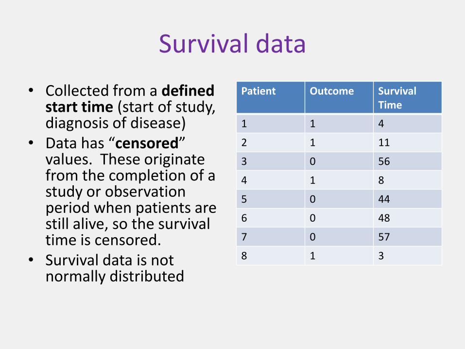
Survival data

• Collected from a defined start time (start of study, diagnosis of disease)

• Data has “censored” values. These originate from the completion of a study or observation period when patients are still alive, so the survival time is censored.

• Survival data is not normally distributed

Patient Outcome SurvivalTime

1 1 4

2 1 11

3 0 56

4 1 8

5 0 44

6 0 48

7 0 57

8 1 3

Survival data

• Two functions are of particular use in survival analyses:

Kaplan-Meier survival function

Cox proportional hazards model

Kaplan Meier Survival

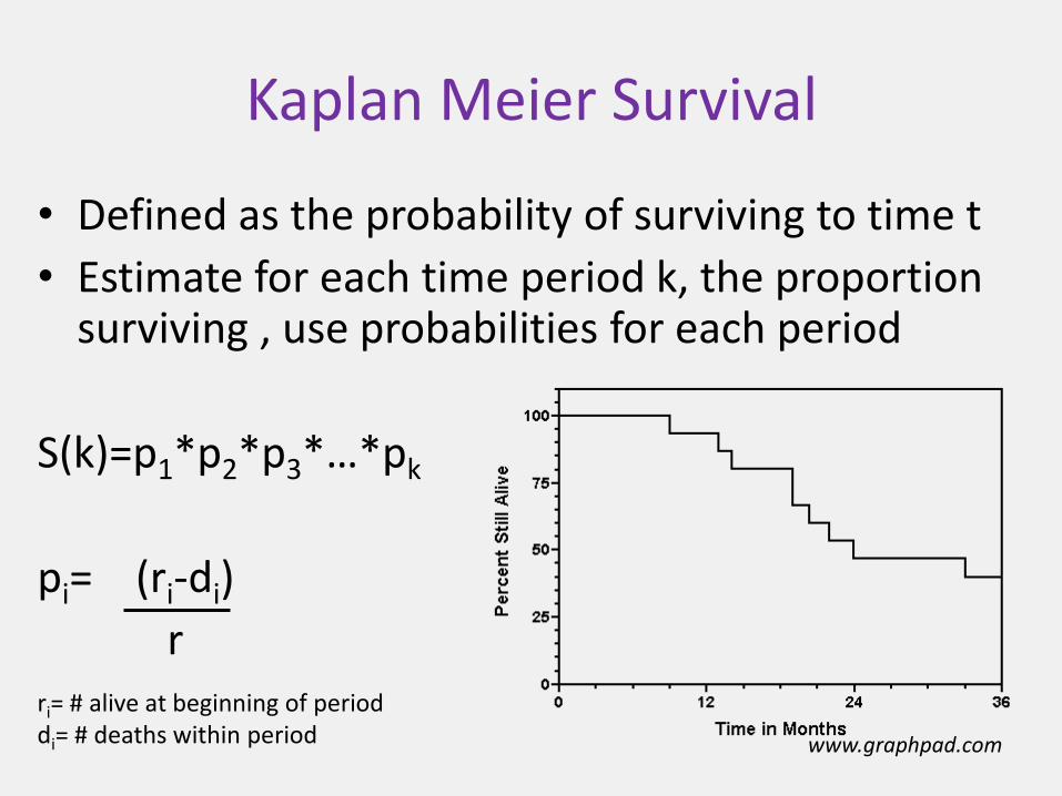
• Defined as the probability of surviving to time t

• Estimate for each time period k, the proportion surviving , use probabilities for each period

S(k)=p1*p2*p3*…*pk

pi= (ri-di)

r

www.graphpad.com

ri= # alive at beginning of perioddi= # deaths within period

Comparing survival curves

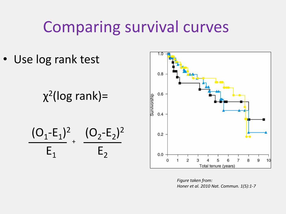
• Use log rank test

χ2(log rank)=

(O1-E1)2 (O2-E2)2

E1 E2

Figure taken from:Honer et al. 2010 Nat. Commun. 1(5):1-7

+

Cox proportional hazards model

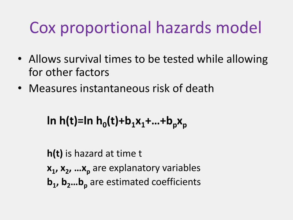
• Allows survival times to be tested while allowing for other factors

• Measures instantaneous risk of death

ln h(t)=ln h0(t)+b1x1+…+bpxp

h(t) is hazard at time t

x1, x2, …xp are explanatory variables

b1, b2…bp are estimated coefficients

Microarray data

• Gene expression

• Survival (0 or 1)

• Survival time

• Various other risk factors (age, sex, experimental or prophylactic treatments, etc.)

• How to incorporate everything into gene expression analyses?

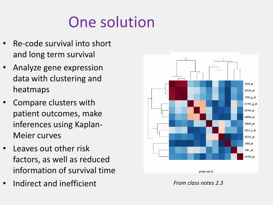
One solution• Re-code survival into short

and long term survival

• Analyze gene expression data with clustering and heatmaps

• Compare clusters with patient outcomes, make inferences using Kaplan-Meier curves

• Leaves out other risk factors, as well as reduced information of survival time

• Indirect and inefficient From class notes 2.3

• Ideally, would like to build a model that incorporates all factors with gene expression as response variable.

Tree Based Ensemble Methods

• Use classification trees

• Tree is built through successive splitting of data into two groups. Xj is splitting covariate, one node contains all Xj<=c and other is all Xj>c.

• Data is continually split until chosen thresholds show that no more splits are desirable.

Ensemble methods:

Bootstrap aggregating

• Need to aggregate predictions of multiple trees to come up with ensemble prediction

• Bootstrap aggregating (bagging)- take bootstrap samples from learning sample, each sample is fitted with a model, aggregate the models by combining classifiers with weights.

• Ensemble predictors will vote for a specific outcome

Ensemble methods:

Bootstrap aggregating

• In survival analysis, we aggregate the observations of the trees, not the predictions

• All observations that were included in same node (0 or 1) are combined and one Kaplan-Meier curve is constructed from those data.

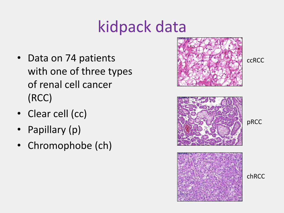
kidpack data

• Data on 74 patients with one of three types of renal cell cancer (RCC)

• Clear cell (cc)

• Papillary (p)

• Chromophobe (ch)

ccRCC

pRCC

chRCC

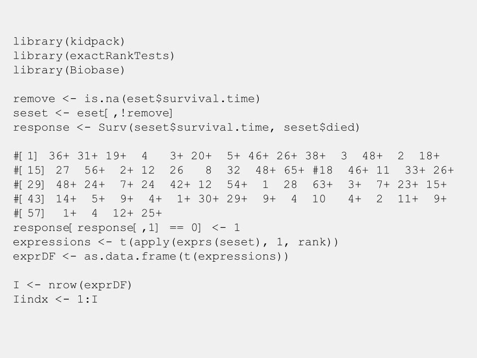
library(kidpack)

library(exactRankTests)

library(Biobase)

remove <- is.na(eset$survival.time)

seset <- eset[,!remove]

response <- Surv(seset$survival.time, seset$died)

#[1] 36+ 31+ 19+ 4 3+ 20+ 5+ 46+ 26+ 38+ 3 48+ 2 18+

#[15] 27 56+ 2+ 12 26 8 32 48+ 65+ #18 46+ 11 33+ 26+

#[29] 48+ 24+ 7+ 24 42+ 12 54+ 1 28 63+ 3+ 7+ 23+ 15+

#[43] 14+ 5+ 9+ 4+ 1+ 30+ 29+ 9+ 4 10 4+ 2 11+ 9+

#[57] 1+ 4 12+ 25+

response[response[,1] == 0] <- 1

expressions <- t(apply(exprs(seset), 1, rank))

exprDF <- as.data.frame(t(expressions))

I <- nrow(exprDF)

Iindx <- 1:I

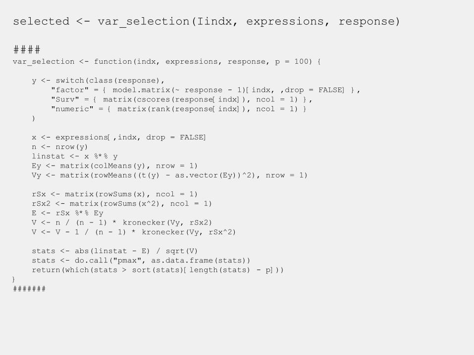
selected <- var_selection(Iindx, expressions, response)

####var_selection <- function(indx, expressions, response, p = 100) {

y <- switch(class(response),

"factor" = { model.matrix(~ response - 1)[indx, ,drop = FALSE] },

"Surv" = { matrix(cscores(response[indx]), ncol = 1) },

"numeric" = { matrix(rank(response[indx]), ncol = 1) }

)

x <- expressions[,indx, drop = FALSE]

n <- nrow(y)

linstat <- x %*% y

Ey <- matrix(colMeans(y), nrow = 1)

Vy <- matrix(rowMeans((t(y) - as.vector(Ey))^2), nrow = 1)

rSx <- matrix(rowSums(x), ncol = 1)

rSx2 <- matrix(rowSums(x^2), ncol = 1)

E <- rSx %*% Ey

V <- n / (n - 1) * kronecker(Vy, rSx2)

V <- V - 1 / (n - 1) * kronecker(Vy, rSx^2)

stats <- abs(linstat - E) / sqrt(V)

stats <- do.call("pmax", as.data.frame(stats))

return(which(stats > sort(stats)[length(stats) - p]))

}

#######

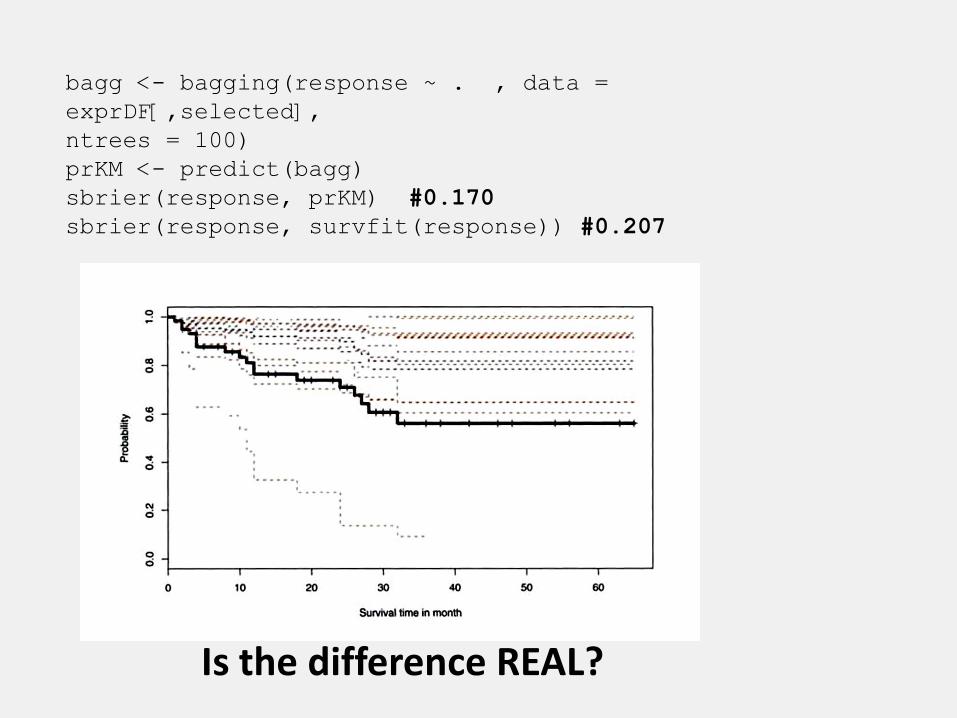
bagg <- bagging(response ~ . , data =

exprDF[,selected],

ntrees = 100)

prKM <- predict(bagg)

sbrier(response, prKM) #0.170

sbrier(response, survfit(response)) #0.207

Is the difference REAL?

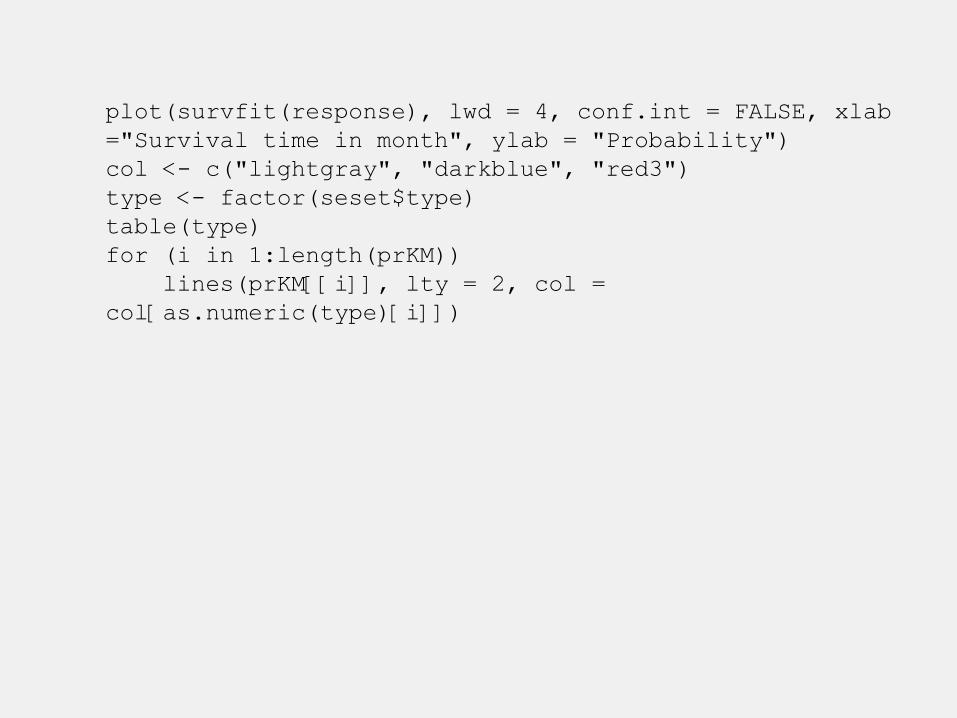
plot(survfit(response), lwd = 4, conf.int = FALSE, xlab

="Survival time in month", ylab = "Probability")

col <- c("lightgray", "darkblue", "red3")

type <- factor(seset$type)

table(type)

for (i in 1:length(prKM))

lines(prKM[[i]], lty = 2, col =

col[as.numeric(type)[i]])

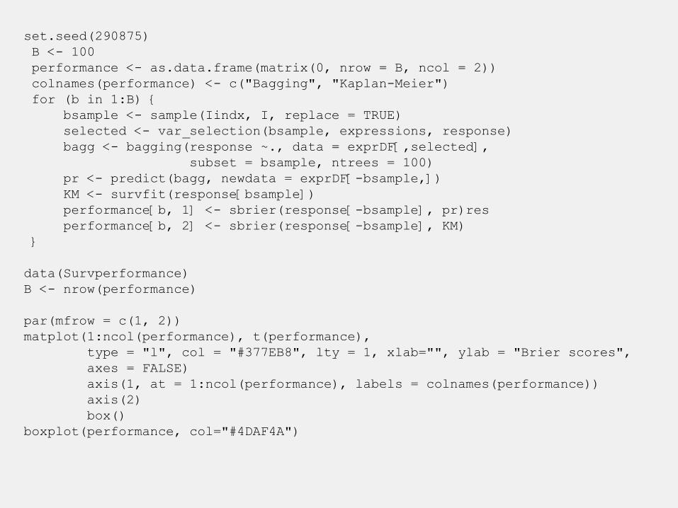
set.seed(290875)

B <- 100

performance <- as.data.frame(matrix(0, nrow = B, ncol = 2))

colnames(performance) <- c("Bagging", "Kaplan-Meier")

for (b in 1:B) {

bsample <- sample(Iindx, I, replace = TRUE)

selected <- var_selection(bsample, expressions, response)

bagg <- bagging(response ~., data = exprDF[,selected],

subset = bsample, ntrees = 100)

pr <- predict(bagg, newdata = exprDF[-bsample,])

KM <- survfit(response[bsample])

performance[b, 1] <- sbrier(response[-bsample], pr)res

performance[b, 2] <- sbrier(response[-bsample], KM)

}

data(Survperformance)

B <- nrow(performance)

par(mfrow = c(1, 2))

matplot(1:ncol(performance), t(performance),

type = "l", col = "#377EB8", lty = 1, xlab="", ylab = "Brier scores",

axes = FALSE)

axis(1, at = 1:ncol(performance), labels = colnames(performance))

axis(2)

box()

boxplot(performance, col="#4DAF4A")

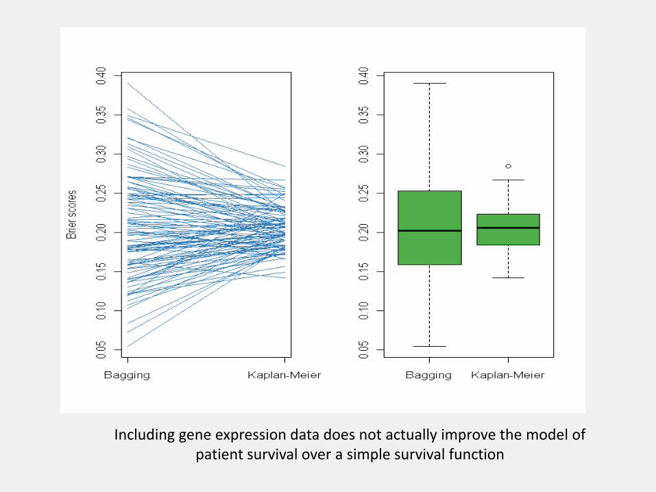
Including gene expression data does not actually improve the model of patient survival over a simple survival function

rbsurv package

• Select survival associated genes based on likelihood function

• Utilizes Cox model

• Employs forward selection

For each sample with x expression values, ytime and δ censoring status:

• Randomly divide samples into training set and validation set. Fit gene to training set, obtain β, evaluate log likelihood with parameter estimate and validation set. Repeat for each gene.

• Repeat B (user selected) times. Select best gene with smallest log likelihood.

• Adjust for best gene. Find the next best gene. • Forward selection until fitting is impossible due to lack

of samples. • Compute AIC for all model, remove model and repeat

steps. • Risk factors can be included in the modeling.

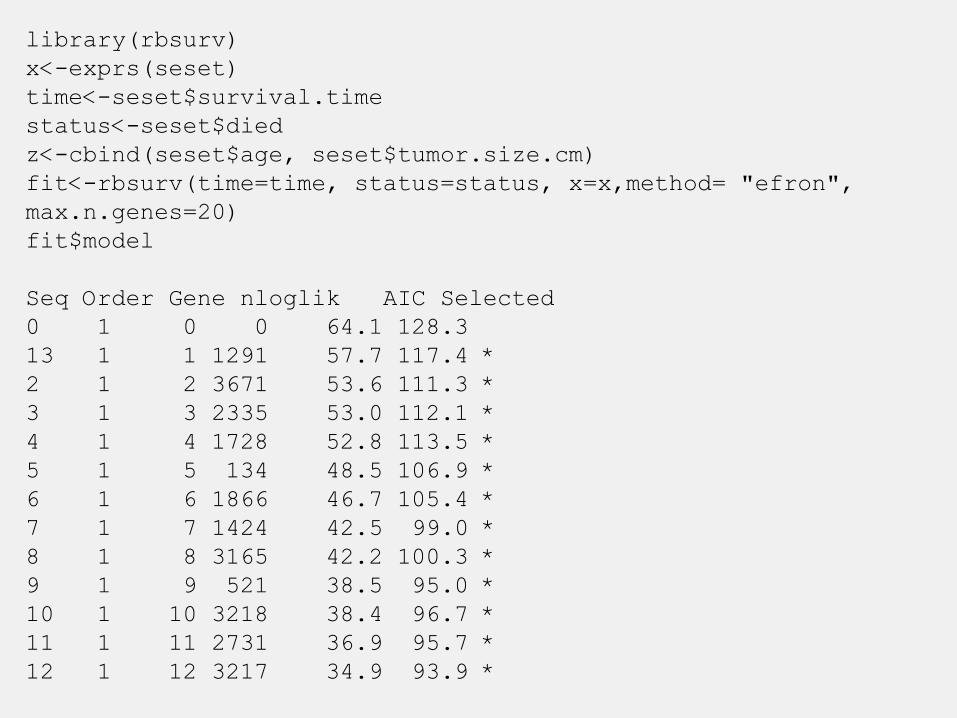
library(rbsurv)

x<-exprs(seset)

time<-seset$survival.time

status<-seset$died

z<-cbind(seset$age, seset$tumor.size.cm)

fit<-rbsurv(time=time, status=status, x=x,method= "efron",

max.n.genes=20)

fit$model

Seq Order Gene nloglik AIC Selected

0 1 0 0 64.1 128.3

13 1 1 1291 57.7 117.4 *

2 1 2 3671 53.6 111.3 *

3 1 3 2335 53.0 112.1 *

4 1 4 1728 52.8 113.5 *

5 1 5 134 48.5 106.9 *

6 1 6 1866 46.7 105.4 *

7 1 7 1424 42.5 99.0 *

8 1 8 3165 42.2 100.3 *

9 1 9 521 38.5 95.0 *

10 1 10 3218 38.4 96.7 *

11 1 11 2731 36.9 95.7 *

12 1 12 3217 34.9 93.9 *

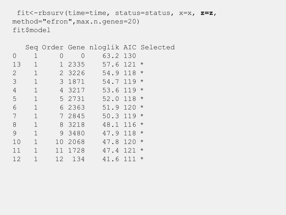
fit<-rbsurv(time=time, status=status, x=x, z=z,

method="efron",max.n.genes=20)

fit$model

Seq Order Gene nloglik AIC Selected

0 1 0 0 63.2 130

13 1 1 2335 57.6 121 *

2 1 2 3226 54.9 118 *

3 1 3 1871 54.7 119 *

4 1 4 3217 53.6 119 *

5 1 5 2731 52.0 118 *

6 1 6 2363 51.9 120 *

7 1 7 2845 50.3 119 *

8 1 8 3218 48.1 116 *

9 1 9 3480 47.9 118 *

10 1 10 2068 47.8 120 *

11 1 11 1728 47.4 121 *

12 1 12 134 41.6 111 *

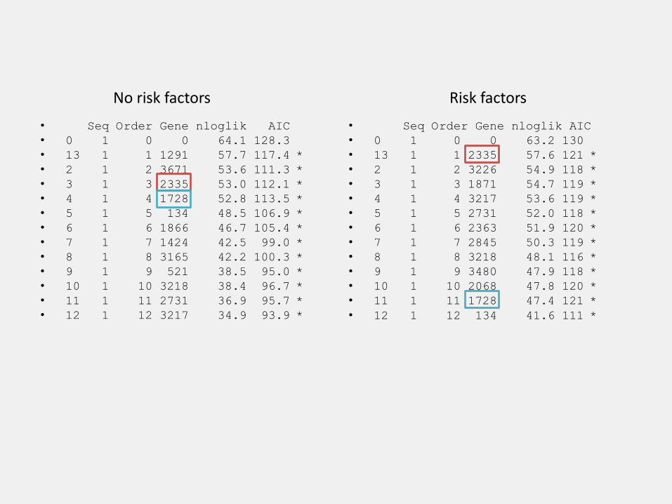
• Seq Order Gene nloglik AIC

• 0 1 0 0 64.1 128.3

• 13 1 1 1291 57.7 117.4 *

• 2 1 2 3671 53.6 111.3 *

• 3 1 3 2335 53.0 112.1 *

• 4 1 4 1728 52.8 113.5 *

• 5 1 5 134 48.5 106.9 *

• 6 1 6 1866 46.7 105.4 *

• 7 1 7 1424 42.5 99.0 *

• 8 1 8 3165 42.2 100.3 *

• 9 1 9 521 38.5 95.0 *

• 10 1 10 3218 38.4 96.7 *

• 11 1 11 2731 36.9 95.7 *

• 12 1 12 3217 34.9 93.9 *

• Seq Order Gene nloglik AIC

• 0 1 0 0 63.2 130

• 13 1 1 2335 57.6 121 *

• 2 1 2 3226 54.9 118 *

• 3 1 3 1871 54.7 119 *

• 4 1 4 3217 53.6 119 *

• 5 1 5 2731 52.0 118 *

• 6 1 6 2363 51.9 120 *

• 7 1 7 2845 50.3 119 *

• 8 1 8 3218 48.1 116 *

• 9 1 9 3480 47.9 118 *

• 10 1 10 2068 47.8 120 *

• 11 1 11 1728 47.4 121 *

• 12 1 12 134 41.6 111 *

No risk factors Risk factors

Summary

• There are many methods for analyzing survival data- these are just two

• Depending upon your desired result and input data, want to choose methods based upon either a survival or hazard function