Embed Size (px)
Citation preview
Swarming Unmanned Aerial Vehicles: Concept Development and Experimentation, A State of the Art Review on Flight and Mission Control
Bumsoo Kim, Paul Hubbard and Dan Necsulescu
Defence R&D Canada √ Ottawa TECHNICAL MEMORANDUM
DRDC Ottawa TM 2003-176 December 2003

Swarming Unmanned Aerial Vehicles: Concept Development and Experimentation, A State of the Art Review on Flight and Mission Control
Bumsoo Kim DRDC Ottawa
Paul Hubbard DRDC Ottawa
Dan Necsulescu University of Ottawa
Defence R&D Canada – Ottawa Technical Memorandum DRDC Ottawa TM 2003-176 December 2004-01-05
© Her Majesty the Queen as represented by the Minister of National Defence, 2003
© Sa majesté la reine, représentée par le ministre de la Défense nationale, 2003
DRDC Ottawa TM 2003-176 i
Abstract
This technical memorandum provides an overview of the state of the art of control system design for swarming UAVs. An overview of trends and future needs for military applications of UAVs is presented first. Linear controller design for aircrafts is then reviewed in the context of UAV systems. Comparative analysis of flight, collision avoidance and mission control approaches for swarming UAVs is provided. Then, advanced nonlinear UAV control designs including several feedback linearization techniques, Neural Network implementation, Fuzzy Logic application incorporated with Linear and Nonlinear Model Predictive Control for swarming UAVs are analysed. Finally, the importance of Hardware in the Loop Simulation is discussed. Simulation and experimental validation results will be presented in subsequent reports.
Résumé
Ce document technique donne une vue d’ensemble de l’état actuel des connaissances en matière de conception des systèmes de commande d’engins télépilotés volant en groupe. Une vue d’ensemble des tendances et des besoins futurs pour les applications militaires des engins télépilotés est d’abord présentée. Une analyse comparative des vols, des évitements d’abordage et des approches relatives au contrôle des missions des engins télépilotés volant en groupe est fournie. Puis, des modèles de contrôle non linéaire évolués pour les engins télépilotés, y compris plusieurs techniques de linéarisation de la rétroaction, la mise en oeuvre de réseaux neuronaux et un application de la logique floue intégrée au contrôle prédictif des modèles linéaires et non linéaires des engins télépilotés volant en groupe sont analysés. Enfin, l’importance du matériel dans la simulation en boucle est abordée. Les résultats des simulations et de la validation des expériences seront présentés dans des rapports subséquents.

ii DRDC Ottawa TM 2003-176
This page intentionally left blank.
DRDC Ottawa TM 2003-176 iii
Executive summary The purpose of this technical memorandum is to provide input to the multi-UAV cooperative control research community on the topic of navigation sensing and control approaches and related communication bandwidth reduction requirements for high-performance flight and mission characteristics for swarming UAVs. Each UAV has local control requirements and the swarming UAVs have supplementary sensing, control and communications requirements imposed due to membership of the UAV swarm. These issues have to be addressed concurrently and for this purpose further research and development work is needed. This report serves as the basis of the research to be performed in our TIF project, “Enabling Aerial Autonomous Intelligent System Cooperation Through A Time-Constrained Decentralized Model Predictive Control”. This report focuses on control approaches for flight control and collision avoidance of swarming UAVs and provides the following:
• A literature review regarding: (a) UAV flight and mission control;
(b) Navigation sensing, control and communication requirements for swarming UAVs;
• A comparative analysis of dynamic, kinematic, geometric, neural networks and fuzzy approaches for flight control and collision avoidance for swarming UAVs.
• A synthesis of the basic control approaches in analytical and block diagram forms An essential step for the research of swarming UAVs was an investigation of the state-of-the-art of development of individual UAV flight and mission control approaches and swarming UAV’s sensing-control and communication approaches as documented in the published literature. The analysis consists of comparison of dynamic, kinematic, geometric, neural networks, and fuzzy logic approaches for flight control and collision avoidance of swarming UAVs. The results of the analysis are presented in the framework of analytical models and block diagrams. The report provides conclusions and recommendations concerning the performance of the proposed approaches in terms of suitability for flight and mission control of swarming UAVs.
Kim, B., Hubbard, P., Necsulescu, D. 2003. Swarming UAV’s Concept Development and Experimentation; A State of the Art Review on Flight and Mission Control. DRDC Ottawa TM 2003-176. Defence R&D Canada - Ottawa.
iv DRDC Ottawa TM 2003-176
Sommaire Ce document technique a pour objet de renseigner le milieu de la recherche sur le contrôle coopératif au sujet de la détection de navigation, des approches relatives au contrôle et des exigences connexes en matière de réduction de la largeur de bande de communication pour les caractéristiques de vol et de mission haute performance des engins télépilotés volant en groupe. Chaque engin télépiloté a des exigences de contrôle local, et les engins télépilotés volant en groupe ont des exigences supplémentaires en matière de détection, de contrôle et de communication qui sont imposées du fait qu’ils volent en groupe. Ces questions doivent être traitées en même temps et, à cette fin, d’autres recherches et du travail de développement sont nécessaires. Ce rapport sert de base à la recherche qui doit être exécutée dans le cadre de notre projet FIT intitulé « Coopération de systèmes intelligents autonomes aériens grâce au contrôle prédictif d’un modèle décentralisé limité dans le temps ». Ce rapport porte sur les approches de contrôle et d’évitement d’abordage d’engins télépilotés volant en groupe et il contient ce qui suit :
• une revue de la documentation portant sur : a) le contrôle du vol et de la mission d’un engin télépiloté; b) les exigences en matière de détection de la navigation, de contrôle et
de communication d’engins télépilotés volant en groupe; • une analyse comparative de la dynamique, de la cinématique, de la
géométrie, des réseaux neuronaux et des approches floues liés au contrôle du vol et à l’évitement des abordages pour les engins télépilotés volant en groupe;
• une synthèse des approches de contrôle fondamentales sous forme analytique et schématique.
Une étape essentielle de la recherche sur les engins télépilotés volant en groupe a été l’examen de l’état des connaissances en matière de développement d’approches de contrôle de vol et de mission d’un engin télépiloté pris isolément ainsi que des approches liées à la communication et au contrôle de détection des engins télépilotés volant en groupe, comme elles figurent dans la documention publiée. L’analyse consiste à comparer la dynamique, la cinématique, la géométrie, les réseaux neuronaux et les approches à logique floue pour le contrôle du vol et l’évitement des abordages des engins télépilotés volant en groupe.
Les résultats de l’analyse sont présentés dans le cadre de modèles analytiques et de schémas de principe. Le rapport contient des conclusions et des recommandations relatives au rendement des approches proposées en termes d’adéquation par rapport au contrôle du vol et des missions des engins télépilotés volant en groupe.
Kim, B., Hubbard, P., Necsulescu, D. 2003. Swarming UAV’s Concept Development and Experimentation; A State of the Art Review on Flight and Mission Control. DRDC Ottawa TM 2003-176 R & D pour la défense Canada - Ottawa.
DRDC Ottawa TM 2003-176 v
Table of contents
Abstract........................................................................................................................................ i
Résumé ........................................................................................................................................ i
Executive summary ................................................................................................................... iii
Sommaire................................................................................................................................... iv
Table of contents ........................................................................................................................ v
List of figures ........................................................................................................................... vii
Acknowledgements .................................................................................................................... x
1. INTRODUCTION................................................................................................................ 1
1.1 Overview of the Unmanned Aerial Vehicles (UAVs) Trends and Future Needs for Military Applications ............................................................................................... 1
1.2 UAV Systems ........................................................................................................ 3
1.3 UAV Models for Controller Design ...................................................................... 6
2. REVIEW OF LINEAR CONTROLLER DESIGN FOR AIRCRAFTS ............................ 11
2.1 Automatic Linear Controller for Stabilization..................................................... 11
2.2 Automatic Linear Controller for Navigation ....................................................... 14
3. COMPARATIVE ANALYSIS OF FLIGHT, COLLISION AVOIDANCE AND MISSION CONTROL APPROACHES FOR SWARMING UAVs........................................ 22
3.1 Typical Approaches for Single UAV Flight Control using Optimal, Neural Networks and Fuzzy Control Methods........................................................................ 22
3.2 Swarming UAVs Approaches for Path Planning with Collision Avoidance with Fixed Obstacles ........................................................................................................... 33
3.3 Swarming UAVs Approaches for Flight Control and Collision Avoidance with Moving Obstacles ........................................................................................................ 38
3.4 Sensing-Communications Requirements for UAVs Control and Collision Avoidance.................................................................................................................... 44
vi DRDC Ottawa TM 2003-176
4. ADVANCED UAV CONTROL DESIGN ISSUES FOR SWARMING UAV’S ............. 46
4.1 Feedback Linearizarion of UAV Nonlinear Dynamics and Controller Design... 46
4.2 Model Predictive Control of UAVs.................................................................... 52
4.3 Digital Simulation and Hardware-in –the Loop Experimentation of Controllers 56
5. CONCLUSIONS AND RECOMMANDATIONS CONCERNING FLIGHT AND MISSION CONTROL OF SWARMING UAVS..................................................................... 61
5.1 Conclusions ......................................................................................................... 61
5.2 Recommendations ............................................................................................... 62
References ................................................................................................................................ 63
List of symbols/abbreviations/acronyms/initialisms ................................................................ 68
DRDC Ottawa TM 2003-176 vii
List of figures
Figure 1.1. UAV conventional flight control system ................................................................ 4
Figure 1.2. Control system of two UAVs with collision avoidance capability ........................ 5
Figure 2.1. Inner Loop Control System.................................................................................. 11
Figure 2.2. Pitch damper......................................................................................................... 12
Figure 2.3. Yaw damper ......................................................................................................... 13
Figure 2.4. Roll damper.......................................................................................................... 13
Figure 2.5. Outer Loop Control System ................................................................................. 14
Figure 2.6. Flight Plan ............................................................................................................ 15
Figure 2.7. UAV commands computation.............................................................................. 16
Figure 2.8. Aerospeed hold..................................................................................................... 17
Figure 2.9. Altitude hold......................................................................................................... 18
Figure 2.10. Turn rate control.................................................................................................. 19
Figure 2.11. Line tracker control ............................................................................................. 20
Figure 3.1. UAV advanced flight controller structure ............................................................ 22
Figure 3.2. LQ optimal control for the inner loop .................................................................. 23
Figure 3.3. LQG optimal controller for the inner loop ........................................................... 24
Figure 3.4. Generic block diagram of a controller using Neural Networks (NN) .................. 26
Figure 3.5. Traffic flow controller using Neural Networks.................................................... 27
Figure 3.6. Model Predictive Controller (MPC) using a Neural Networks model ................. 28
Figure 3.7. Self-tuning regulator using a Neural Nwtworks model........................................ 28
Figure 3.8. Heading controller using gain scheduling based on a NN model ........................ 29
Figure 3.9. UAV flight control using NN............................................................................... 29
Figure 3.10. Basic Fuzzy controller.......................................................................................... 30
viii DRDC Ottawa TM 2003-176
Figure 3.11. Autotuned Fuzzy controller.................................................................................. 31
Figure 3.12. Autotuned Fuzzy controller for guidance............................................................. 32
Figure 3.13. Block diagram for Proportional Navigation Guidance without obstacles............ 35
Figure 3.14. Block diagram for flight control and collision avoidance with fixed obstacles, unknown at path planning stage ........................................................................................ 36
Figure 3.15. Block diagram for the simulation of collision avoidance with fixed obstacles.... 37
Figure 3.16. Generic block diagram for collision avoidance for multiple UAVs..................... 38
Figure 3.17. Block diagram for the control of the relative distance between two spacecrafts . 40
Figure 3.18. Block diagram for the LQ control of the relative distance between two spacecrafts ......................................................................................................................... 41
Figure 3.19. Block diagram for the PI control of the relative distance between two aircrafts in tight formation flight ......................................................................................................... 42
Figure 3.20. Sensing-Communication requirements for the control of multi UAVs................ 44
Figure 4.1. Vertical position hold using a magnetic suspension system ................................ 47
Figure 4.2. Feedback linearization scheme for vertical position hold of a magnetically levitated mass .................................................................................................................... 48
Figure 4.3. Generic diagram for dynamic inversion............................................................... 50
Figure 4.4. 1 D dynamic inversion of UAV flight dynamics ................................................. 52
Figure 4.5. Generic diagram for MPC for path-flight control ................................................ 54
Figure 4.6. Generic diagram for MPC for heading control of multi-vehicles and multi-targets ........................................................................................................................................... 55
Figure 4.7. Generic block diagram of a conventional HIL simulation setup.......................... 58
Figure 4.8. Generic block diagram of an advanced HIL simulation setup ............................. 59
Figure 4.9. HIL setup with simulated load ............................................................................. 60

DRDC Ottawa TM 2003-176 ix
Acknowledgements
The Authors would like to express thanks to Dr. John Bovenkamp and Dr. Andrew Vallerand for their guidance and support and encouragements on this work, and Dr. Paul Pace for many useful discussions and advices through his deep knowledge and dedication in the UAV research area. Special thanks go to the colleagues in FFSE/DRDC-Ottawa for their friendship, encouragements, fruitful criticism, and smiles.

x DRDC Ottawa TM 2003-176
This page intentionally left blank.
DRDC-Ottawa TR 2003-176 1
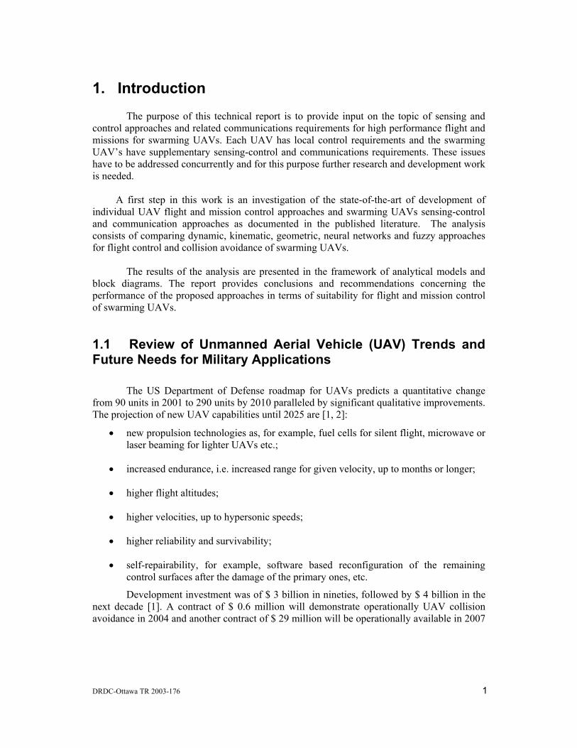
1. Introduction The purpose of this technical report is to provide input on the topic of sensing and control approaches and related communications requirements for high performance flight and missions for swarming UAVs. Each UAV has local control requirements and the swarming UAV’s have supplementary sensing-control and communications requirements. These issues have to be addressed concurrently and for this purpose further research and development work is needed. A first step in this work is an investigation of the state-of-the-art of development of individual UAV flight and mission control approaches and swarming UAVs sensing-control and communication approaches as documented in the published literature. The analysis consists of comparing dynamic, kinematic, geometric, neural networks and fuzzy approaches for flight control and collision avoidance of swarming UAVs. The results of the analysis are presented in the framework of analytical models and block diagrams. The report provides conclusions and recommendations concerning the performance of the proposed approaches in terms of suitability for flight and mission control of swarming UAVs.
1.1 Review of Unmanned Aerial Vehicle (UAV) Trends and Future Needs for Military Applications The US Department of Defense roadmap for UAVs predicts a quantitative change from 90 units in 2001 to 290 units by 2010 paralleled by significant qualitative improvements. The projection of new UAV capabilities until 2025 are [1, 2]:
• new propulsion technologies as, for example, fuel cells for silent flight, microwave or laser beaming for lighter UAVs etc.;
• increased endurance, i.e. increased range for given velocity, up to months or longer;
• higher flight altitudes;
• higher velocities, up to hypersonic speeds;
• higher reliability and survivability;
• self-repairability, for example, software based reconfiguration of the remaining control surfaces after the damage of the primary ones, etc.
Development investment was of $ 3 billion in nineties, followed by $ 4 billion in the next decade [1]. A contract of $ 0.6 million will demonstrate operationally UAV collision avoidance in 2004 and another contract of $ 29 million will be operationally available in 2007
2 DRDC Ottawa TM 2003-176
for autonomous control with automatic collision avoidance, self-adapting flight path and navigation for multi-UAVs [1]. Currently, there are two types of UAVs [2, 15];
• remotely piloted vehicle (RPV); • autonomous or pre-programmed.
RPVs are controlled manually with a stick from a Ground Control Station (GCS) by a pilot trained operator-in-the-loop [2]. An example of a RPV is the Predator, an UAV that can operate 24 hours, flying in a straight line up to 400 miles away from the GCS at a medium-altitude (15,000 ft, up to maximum 25,000 ft). The time delay between the GCS operator command and Predator command execution is a fraction of a second. For this reason, two airplanes (two Predators or a Predator and a manned aircraft) operating in the same area have to maintain a significant clearance to avoid collision. As a medium-altitude UAV, Predator flies at a height range used by manned aircraft. Moreover, multiple Predators controlled by an operator-in-the-loop require significant bandwidth for monitoring and control. Out of 60 units, 19 have been lost because of mishaps or over enemy territory. Operator errors typically occur at landing. Position and orientation of the aircraft with regard to the ground is not available to the operator for landing and landing failures often occur. During flight, if the communication and control between the GCS and the aircraft is lost, the aircraft is commanded to start to fly back home, but without possibility to be monitored and with limited capability to succeed. Autonomous or pre-programmed UAVs use an onboard automatic-controller-in-the-loop for guidance and navigation. Monitoring and mission command modifications are achieved off-line by the operator of the GCS. An example of an autonomous UAV is Global Hawk, a UAV that can operate 35 hours, flying on a given path, along given way points, at a high-altitude (over 65,000 ft)[2]. In this case, two airplanes can operate in the same area maintaining a significant clearance to avoid collision. As a high-altitude UAV, Global Hawk flies at a height range above that used by manned aircraft. Global Hawk achieved across-Atlantic and across-Pacific autonomous flights [2]. Multiple UAVs operating in the same environment with other military airborne and ground vehicles and systems require development for improving mission effectiveness, conceptualization of future capabilities, training of future force etc. These tasks require a synthetic environment containing cooperative models of UAVs, other military airborne and ground vehicles and systems. The result can be an integrated air picture [3, 5]. Multiple UAVs operating in the same environment can be described as swarming UAVs. In general, swarming entities represent autonomous units that can gather from different locations, act together and then disperse [4]. Swarming entities are decentralized, are tolerant to variances of the units or to addition/deletion of units [4]. The behavior of swarming entities can be adopted as a model for coordinating multiple UAVs. For the simulation of UAVs and of the environment for reconnaissance and surveillance a typical system is the Multiple Unified Simulation Environment (MUSE) used by DoD [6]. UAVs simulated are Predator, Hunter, Shadow and Pioneer. The simulator contains 6-DOF models of these UAVs and the data link including the sensors controlled from the Ground Station. The 6-DOF autopilot model has inputs regarding min/max air speeds, climb and turn rates etc.
DRDC Ottawa TM 2003-176 3
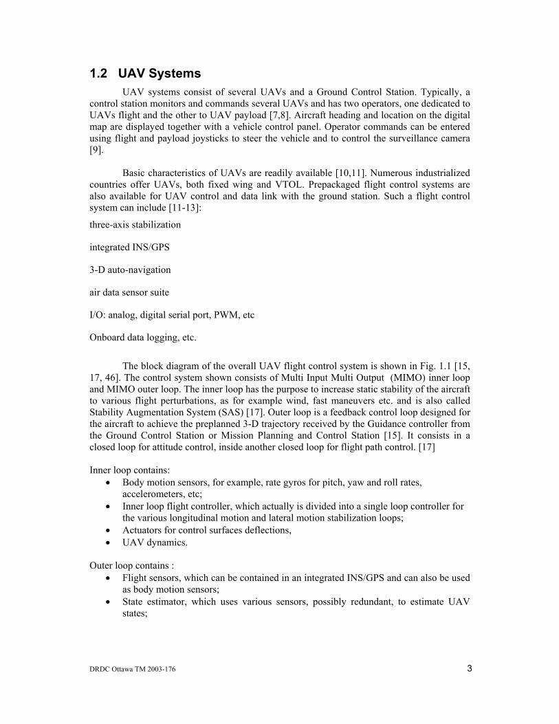
1.2 UAV Systems UAV systems consist of several UAVs and a Ground Control Station. Typically, a control station monitors and commands several UAVs and has two operators, one dedicated to UAVs flight and the other to UAV payload [7,8]. Aircraft heading and location on the digital map are displayed together with a vehicle control panel. Operator commands can be entered using flight and payload joysticks to steer the vehicle and to control the surveillance camera [9]. Basic characteristics of UAVs are readily available [10,11]. Numerous industrialized countries offer UAVs, both fixed wing and VTOL. Prepackaged flight control systems are also available for UAV control and data link with the ground station. Such a flight control system can include [11-13]:
three-axis stabilization
integrated INS/GPS
3-D auto-navigation
air data sensor suite
I/O: analog, digital serial port, PWM, etc
Onboard data logging, etc.
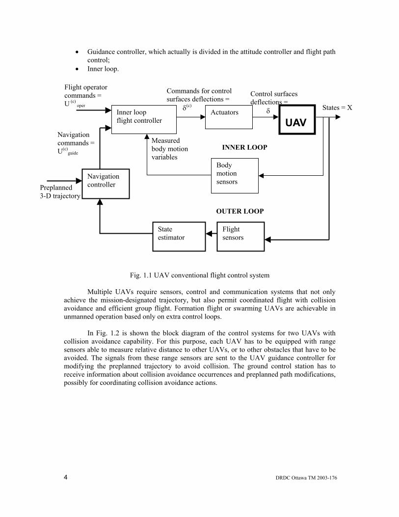
The block diagram of the overall UAV flight control system is shown in Fig. 1.1 [15, 17, 46]. The control system shown consists of Multi Input Multi Output (MIMO) inner loop and MIMO outer loop. The inner loop has the purpose to increase static stability of the aircraft to various flight perturbations, as for example wind, fast maneuvers etc. and is also called Stability Augmentation System (SAS) [17]. Outer loop is a feedback control loop designed for the aircraft to achieve the preplanned 3-D trajectory received by the Guidance controller from the Ground Control Station or Mission Planning and Control Station [15]. It consists in a closed loop for attitude control, inside another closed loop for flight path control. [17] Inner loop contains:
• Body motion sensors, for example, rate gyros for pitch, yaw and roll rates, accelerometers, etc;
• Inner loop flight controller, which actually is divided into a single loop controller for the various longitudinal motion and lateral motion stabilization loops;
• Actuators for control surfaces deflections, • UAV dynamics.
Outer loop contains :
• Flight sensors, which can be contained in an integrated INS/GPS and can also be used as body motion sensors;
• State estimator, which uses various sensors, possibly redundant, to estimate UAV states;
4 DRDC Ottawa TM 2003-176
• Guidance controller, which actually is divided in the attitude controller and flight path control;
• Inner loop.
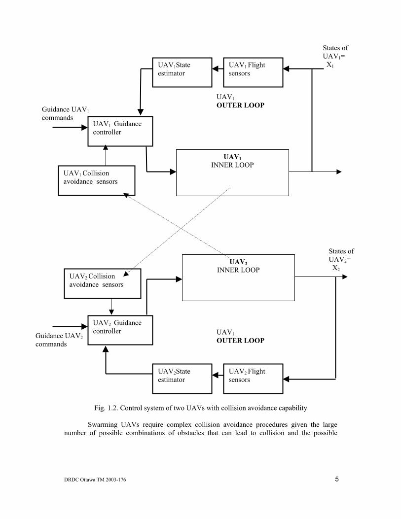
Fig. 1.1 UAV conventional flight control system Multiple UAVs require sensors, control and communication systems that not only achieve the mission-designated trajectory, but also permit coordinated flight with collision avoidance and efficient group flight. Formation flight or swarming UAVs are achievable in unmanned operation based only on extra control loops. In Fig. 1.2 is shown the block diagram of the control systems for two UAVs with collision avoidance capability. For this purpose, each UAV has to be equipped with range sensors able to measure relative distance to other UAVs, or to other obstacles that have to be avoided. The signals from these range sensors are sent to the UAV guidance controller for modifying the preplanned trajectory to avoid collision. The ground control station has to receive information about collision avoidance occurrences and preplanned path modifications, possibly for coordinating collision avoidance actions.
UAV States = X
INNER LOOP
Actuators
Control surfaces deflections = δ
Body motion sensors
Commands for control surfaces deflections = δ(c)
Inner loop flight controller
Measured body motion variables
Flight sensors
State estimator
OUTER LOOP
Navigation controller Preplanned
3-D trajectory
Navigation commands = U(c)
guide
Flight operator commands = U (c)
oper
DRDC Ottawa TM 2003-176 5
Fig. 1.2. Control system of two UAVs with collision avoidance capability Swarming UAVs require complex collision avoidance procedures given the large number of possible combinations of obstacles that can lead to collision and the possible
States of UAV1= X1
UAV1 INNER LOOP
UAV1 Flight sensors
UAV1State estimator
UAV1 OUTER LOOP
UAV1 Guidance controller
Guidance UAV1 commands
States of UAV2= X2
UAV2 INNER LOOP
UAV2 Flight sensors
UAV2State estimator
UAV1 OUTER LOOP
UAV2 Guidance controller Guidance UAV2
commands
UAV2 Collision avoidance sensors
UAV1 Collision avoidance sensors
6 DRDC Ottawa TM 2003-176
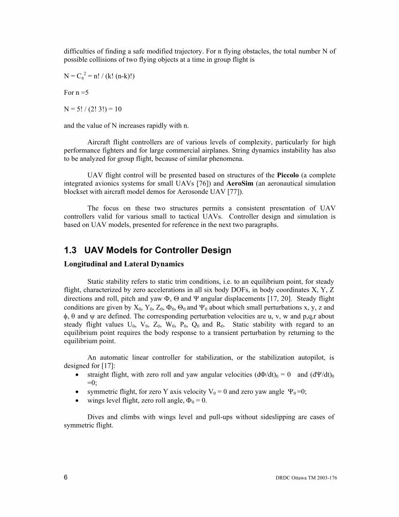
difficulties of finding a safe modified trajectory. For n flying obstacles, the total number N of possible collisions of two flying objects at a time in group flight is N = Cn
2 = n! / (k! (n-k)!) For n =5 N = 5! / (2! 3!) = 10 and the value of N increases rapidly with n. Aircraft flight controllers are of various levels of complexity, particularly for high performance fighters and for large commercial airplanes. String dynamics instability has also to be analyzed for group flight, because of similar phenomena. UAV flight control will be presented based on structures of the Piccolo (a complete integrated avionics systems for small UAVs [76]) and AeroSim (an aeronautical simulation blockset with aircraft model demos for Aerosonde UAV [77]). The focus on these two structures permits a consistent presentation of UAV controllers valid for various small to tactical UAVs. Controller design and simulation is based on UAV models, presented for reference in the next two paragraphs.
1.3 UAV Models for Controller Design Longitudinal and Lateral Dynamics Static stability refers to static trim conditions, i.e. to an equilibrium point, for steady flight, characterized by zero accelerations in all six body DOFs, in body coordinates X, Y, Z directions and roll, pitch and yaw Φ, Θ and Ψ angular displacements [17, 20]. Steady flight conditions are given by X0, Y0, Z0, Φ0, Θ0 and Ψ0 about which small perturbations x, y, z and φ, θ and ψ are defined. The corresponding perturbation velocities are u, v, w and p,q,r about steady flight values U0, V0, Z0, W0, P0, Q0 and R0. Static stability with regard to an equilibrium point requires the body response to a transient perturbation by returning to the equilibrium point. An automatic linear controller for stabilization, or the stabilization autopilot, is designed for [17]:
• straight flight, with zero roll and yaw angular velocities (dΦ/dt)0 = 0 and (dΨ/dt)0 =0;
• symmetric flight, for zero Y axis velocity V0 = 0 and zero yaw angle Ψ0 =0; • wings level flight, zero roll angle, Φ0 = 0.
Dives and climbs with wings level and pull-ups without sideslipping are cases of symmetric flight.
DRDC Ottawa TM 2003-176 7
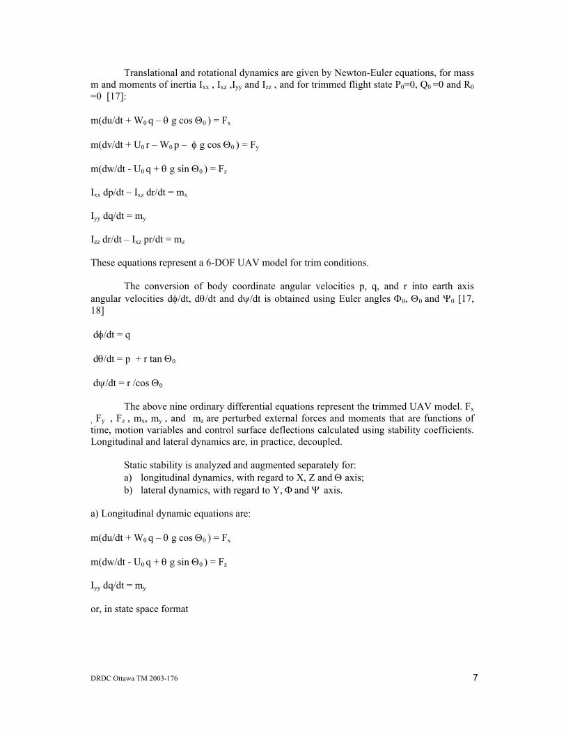
Translational and rotational dynamics are given by Newton-Euler equations, for mass m and moments of inertia Ixx , Ixz ,Iyy and Izz , and for trimmed flight state P0=0, Q0 =0 and R0 =0 [17]: m(du/dt + W0 q – θ g cos Θ0 ) = Fx m(dv/dt + U0 r – W0 p – φ g cos Θ0 ) = Fy m(dw/dt - U0 q + θ g sin Θ0 ) = Fz Ixx dp/dt – Ixz dr/dt = mx Iyy dq/dt = my Izz dr/dt – Ixz pr/dt = mz These equations represent a 6-DOF UAV model for trim conditions. The conversion of body coordinate angular velocities p, q, and r into earth axis angular velocities dφ/dt, dθ/dt and dψ/dt is obtained using Euler angles Φ0, Θ0 and Ψ0 [17, 18] dφ/dt = q dθ/dt = p + r tan Θ0 dψ/dt = r /cos Θ0 The above nine ordinary differential equations represent the trimmed UAV model. Fx
, Fy , Fz , mx, my , and mz are perturbed external forces and moments that are functions of time, motion variables and control surface deflections calculated using stability coefficients. Longitudinal and lateral dynamics are, in practice, decoupled. Static stability is analyzed and augmented separately for:
a) longitudinal dynamics, with regard to X, Z and Θ axis; b) lateral dynamics, with regard to Y, Φ and Ψ axis.
a) Longitudinal dynamic equations are: m(du/dt + W0 q – θ g cos Θ0 ) = Fx m(dw/dt - U0 q + θ g sin Θ0 ) = Fz Iyy dq/dt = my or, in state space format
8 DRDC Ottawa TM 2003-176
du/dt = - W0 q +θ g cos Θ0 + Fx /m dw/dt = U0 q - θ g sin Θ0 + Fz /m dq/dt = my / Iyy dθ/dt = q where, external perturbation forces Fx and Fz and moment my are linearly approximated from a Taylor series by using significant stability derivatives: Xu = (1/m) d Fx / du Xw = (1/m) d Fx / dw Xδth = (1/m) dFx / dδth Zu = (1/m) dFz / du Zw = (1/m) dFz / dw ZδE = (1/m) dFz / dδE Zδth = (1/m) dFz / dδth Mu = (1/ Iyy) dmy / du Mw = (1/ Iyy) dmy / dw Mdw/dt = (1/ Iyy) dmy / d(dw/dt) Mq= (1/ Iyy) dmy / dq MδE = (1/ Iyy) dmy / dδE Mδth = (1/ Iyy) dmy / dδth where δE is elevator deflection and δth is the change of thrust. State equations for longitudinal dynamics become: du/dt = - W0 q +θ g cos Θ0 + Xu u + Xw w + Xδth δth dw/dt = U0 q - θ g sin Θ0 + Zu u + Zw w+ ZδE δE + Zδth δth dq/dt = Mu u + Mww + Mdw/dt (dw/dt) + Mq q+ MδE δE + Mδth δth
DRDC Ottawa TM 2003-176 9
dθ/dt = q or, in state space matrix form [17]: dxL/dt = AL xL + BL uL yL = CL xL where, the state vector is xL = [u w q θ]T the output vector is chosen yL = [δE δth ] T and the matrices AL, BL and CL result directly from the above four state equations. From the above state space equation we can calculate the transfer function u(s) / δE (s). A fixed wing aircraft containing a positive zero indicates a nonminimum phase system. In this case a step input δE (s) results in a undershooting u(t). Open loop dynamics of UAV with limited static stability containing nonminimum phase subsystems can be improved by stability augmentation closed loop systems as part of the autopilots. ) Lateral dynamic equations are: m(dv/dt + U0 r – W0 p – φ g cos Θ0 ) = Fy Ixx dp/dt – Ixz dr/dt = mx Izz dr/dt – Ixz pr/dt = mz d φ / dt = p + r tan Θ0 dψ/dt = r /cos Θ0 Using the same sequence of operations as for the longitudinal dynamic equations, the state space matrix form is obtained as [17]: Dxl/dt = Al xl + Bl ul yl = CL xl where, the state vector is xl = [v p r φ ψ]T the output vector can be chosen as chosen
10 DRDC Ottawa TM 2003-176
yl = [δA δR ] T where δA is aileron deflection and δR is rudder deflection. Similarly, matrices Al, Bl and Cl result from the above five state equations [17].
UAV 6-DOF Model for Trim Conditions in Matrix Form Combining the above longitudinal and lateral dynamics equations, the overall trim condition equations for a 6-DOF UAV model result as, dx/dt = A x + Bu y = C x where, the state vector is x = [u w q θ v p r φ ψ]T the output vector can be chosen as y = [δE δth δA δR] T and matrices A, B and C result directly from the above AL, BL and CL and Al, Bl and Cl matrices. This linear model for trim conditions can be seen as a linearized form of the UAV 6-DOF nonlinear model [17, 18, 75] dx/dt = f(x) + g( x) u y = g (x) The UAV 6-DOF Model for Trim Conditions is used for the design of linear UAV controllers, while the nonlinear one is used for the design of nonlinear controllers and for the test of controllers in simulations.
DRDC Ottawa TM 2003-176 11
2. Review of Linear Controller Design for Aircraft
2.1 Automatic Linear Controllers for Stabilization
Inner Loop Control System
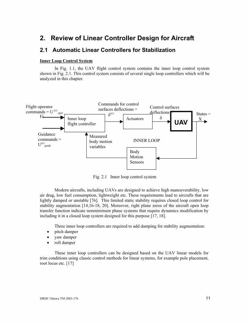
In Fig. 1.1, the UAV flight control system contains the inner loop control system shown in Fig. 2.1. This control system consists of several single loop controllers which will be analyzed in this chapter.
Fi
Fig. 2.1 Inner loop control system
Modern aircrafts, including UAVs are designed to achieve high maneuverability, low air drag, low fuel consumption, lightweight etc. These requirements lead to aircrafts that are lightly damped or unstable [76]. This limited static stability requires closed loop control for stability augmentation [14,16-18, 20]. Moreover, right plane zeros of the aircraft open loop transfer function indicate nonminimum phase systems that require dynamics modification by including it in a closed loop system designed for this purpose [17, 18]. Three inner loop controllers are required to add damping for stability augmentation:
• pitch damper • yaw damper • roll damper
These inner loop controllers can be designed based on the UAV linear models for trim conditions using classic control methods for linear systems, for example pole placement, root locus etc. [17]
UAV States = X
INNER LOOP
Actuators
Control surfaces deflections = δ
Body Motion Sensors
Commands for control surfaces deflections = δ(c)
Inner loop flight controller
Measured body motion variables
Guidance commands = U(c)
guide
Flight operator commands = U (c)
oper
12 DRDC Ottawa TM 2003-176
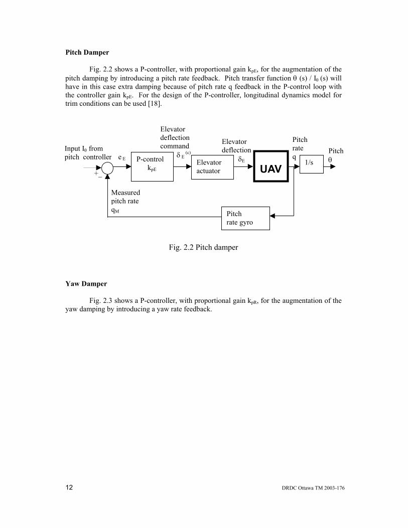
Pitch Damper
Fig. 2.2 shows a P-controller, with proportional gain kpE, for the augmentation of the pitch damping by introducing a pitch rate feedback. Pitch transfer function θ (s) / Iθ (s) will have in this case extra damping because of pitch rate q feedback in the P-control loop with the controller gain kpE. For the design of the P-controller, longitudinal dynamics model for trim conditions can be used [18].
Fig. 2.2 Pitch damper
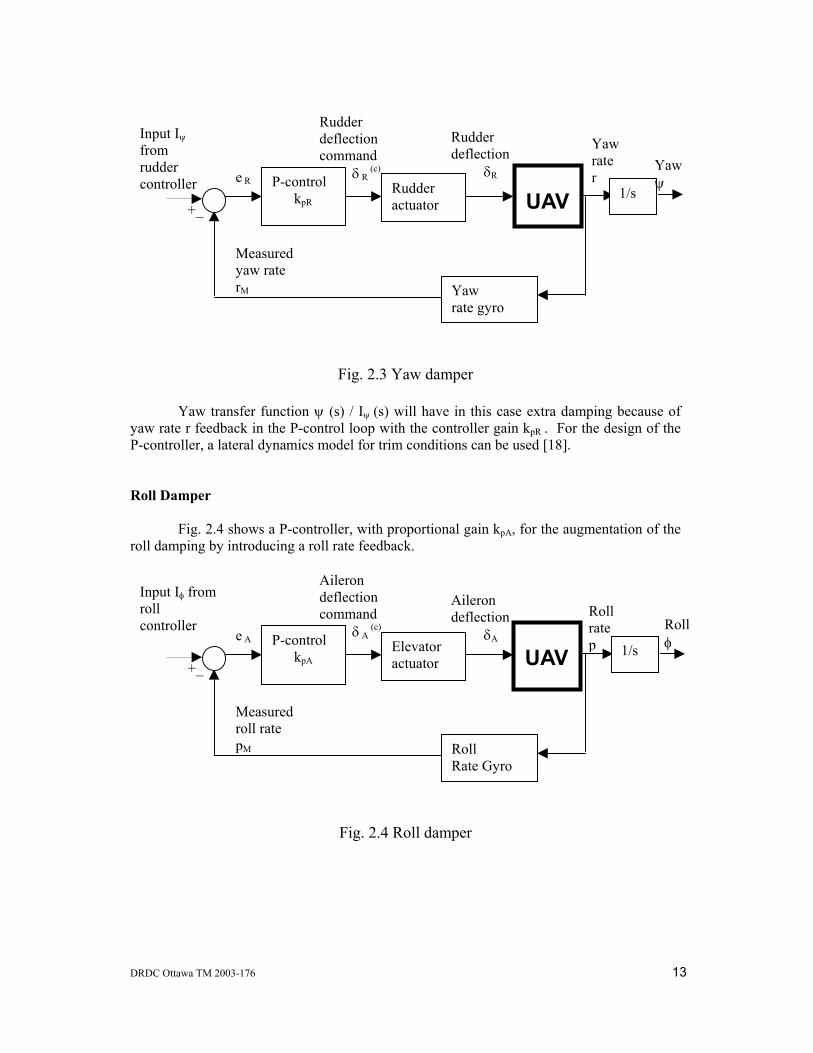
Yaw Damper
Fig. 2.3 shows a P-controller, with proportional gain kpR, for the augmentation of the yaw damping by introducing a yaw rate feedback.
UAV
Pitch rate q
Elevator actuator
Elevator deflection δE
Pitch rate gyro
Elevator deflection command δ E
(c)P-control kpE
Measured pitch rate qM
Input Iθ from pitch controller
+_
e E
1/s Pitch θ
DRDC Ottawa TM 2003-176 13
Fig. 2.3 Yaw damper
Yaw transfer function ψ (s) / Iψ (s) will have in this case extra damping because of yaw rate r feedback in the P-control loop with the controller gain kpR . For the design of the P-controller, a lateral dynamics model for trim conditions can be used [18].
Roll Damper
Fig. 2.4 shows a P-controller, with proportional gain kpA, for the augmentation of the roll damping by introducing a roll rate feedback.
Fig. 2.4 Roll damper
UAV
Yaw rate r
Rudder actuator
Rudder deflection δR
Yaw rate gyro
Rudder deflection command δ R
(c)P-control kpR
Measured yaw rate rM
Input Iψ from rudder controller
+_
e R
1/s
Yaw ψ
UAV
Roll rate p Elevator
actuator
Aileron deflection δA
Roll Rate Gyro
Aileron deflection command δ A
(c)P-control kpA
Measured roll rate pM
Input Iφ from roll controller
+_
e A
1/s
Roll φ
14 DRDC Ottawa TM 2003-176
Roll transfer function φ (s) / Iφ (s) will have in this case extra damping because of roll rate p feedback in the P-control loop with the controller gain kpA. For the design of the P-controler, lateral dynamics model for trim conditions can be used [18].
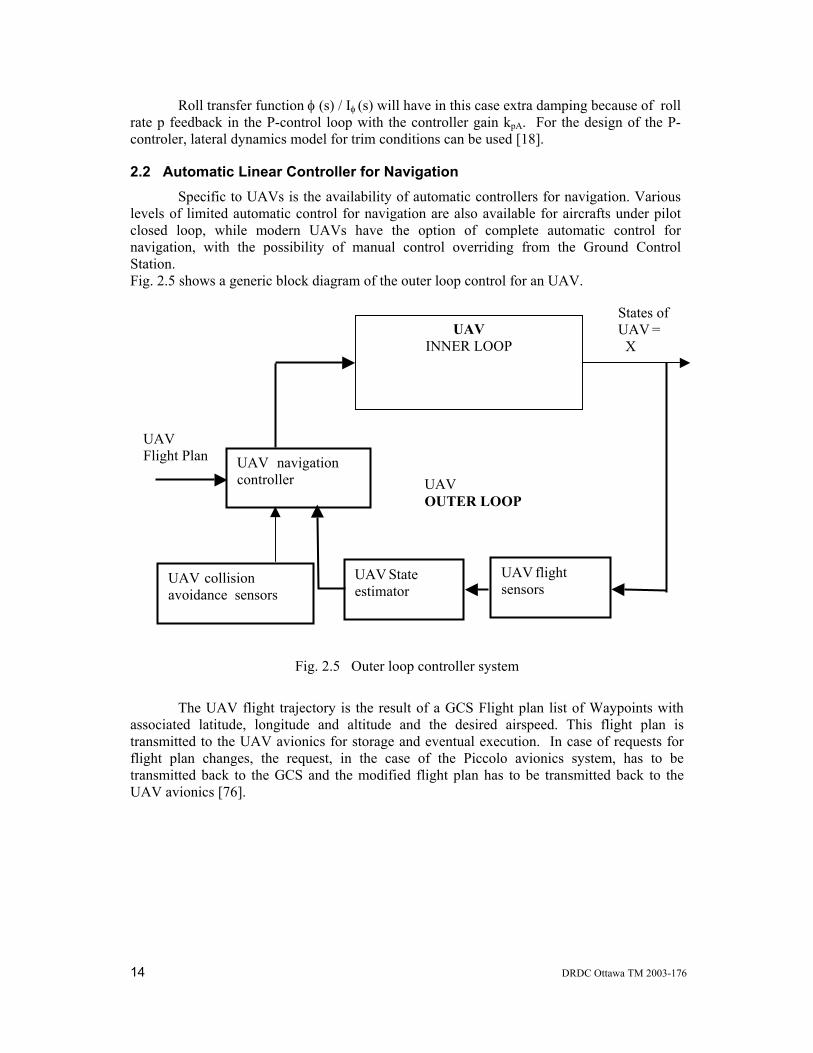
2.2 Automatic Linear Controller for Navigation Specific to UAVs is the availability of automatic controllers for navigation. Various levels of limited automatic control for navigation are also available for aircrafts under pilot closed loop, while modern UAVs have the option of complete automatic control for navigation, with the possibility of manual control overriding from the Ground Control Station. Fig. 2.5 shows a generic block diagram of the outer loop control for an UAV.
Fig. 2.5 Outer loop controller system
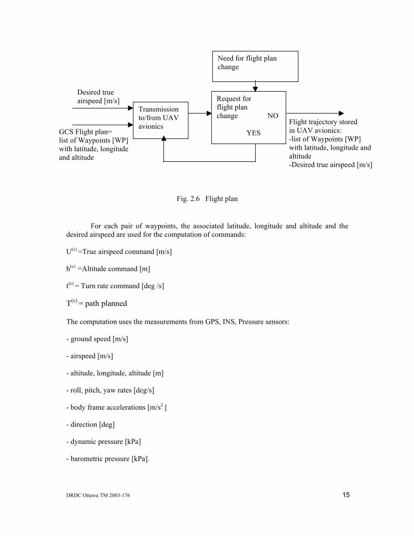
The UAV flight trajectory is the result of a GCS Flight plan list of Waypoints with associated latitude, longitude and altitude and the desired airspeed. This flight plan is transmitted to the UAV avionics for storage and eventual execution. In case of requests for flight plan changes, the request, in the case of the Piccolo avionics system, has to be transmitted back to the GCS and the modified flight plan has to be transmitted back to the UAV avionics [76].
States of UAV = X
UAV INNER LOOP
UAV flight sensors
UAV State estimator
UAV OUTER LOOP
UAV navigation controller
UAV Flight Plan
UAV collision avoidance sensors
DRDC Ottawa TM 2003-176 15
Fig. 2.6 Flight plan
For each pair of waypoints, the associated latitude, longitude and altitude and the desired airspeed are used for the computation of commands: U(c) =True airspeed command [m/s]
h(c) =Altitude command [m]
t(c) = Turn rate command [deg /s]
T(c) = path planned
The computation uses the measurements from GPS, INS, Pressure sensors:
- ground speed [m/s]
- airspeed [m/s]
- altitude, longitude, altitude [m]
- roll, pitch, yaw rates [deg/s]
- body frame accelerations [m/s2 ]
- direction [deg]
- dynamic pressure [kPa]
- barometric pressure [kPa].
GCS Flight plan= list of Waypoints [WP] with latitude, longitude and altitude
Transmission to/from UAV avionics
Desired true airspeed [m/s] Request for
flight plan change NO YES
Flight trajectory stored in UAV avionics: -list of Waypoints [WP] with latitude, longitude and altitude -Desired true airspeed [m/s]
Need for flight plan change
16 DRDC Ottawa TM 2003-176
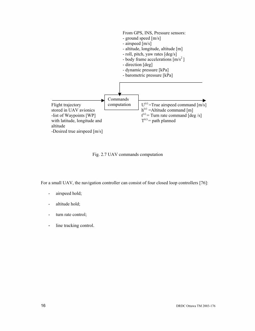
Fig. 2.7 UAV commands computation
For a small UAV, the navigation controller can consist of four closed loop controllers [76]:
- airspeed hold;
- altitude hold;
- turn rate control;
- line tracking control.
U(c) =True airspeed command [m/s] h(c) =Altitude command [m] t(c) = Turn rate command [deg /s] T(c) = path planned
Flight trajectory stored in UAV avionics -list of Waypoints [WP] with latitude, longitude and altitude -Desired true airspeed [m/s]
Commands computation
From GPS, INS, Pressure sensors: - ground speed [m/s] - airspeed [m/s] - altitude, longitude, altitude [m] - roll, pitch, yaw rates [deg/s] - body frame accelerations [m/s2 ]
- direction [deg] - dynamic pressure [kPa] - barometric pressure [kPa]
DRDC Ottawa TM 2003-176 17
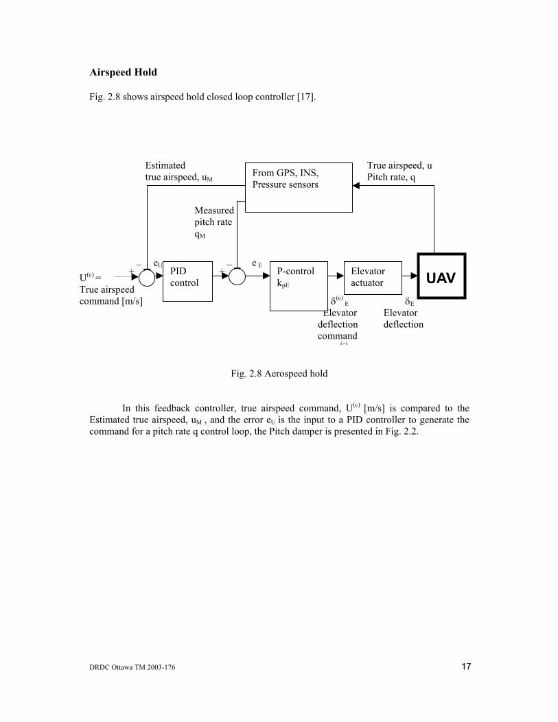
Airspeed Hold
Fig. 2.8 shows airspeed hold closed loop controller [17].
Fig. 2.8 Aerospeed hold
In this feedback controller, true airspeed command, U(c) [m/s] is compared to the Estimated true airspeed, uM , and the error eU is the input to a PID controller to generate the command for a pitch rate q control loop, the Pitch damper is presented in Fig. 2.2.
U(c) = True airspeed command [m/s]
UAVElevator actuator
δE Elevator deflection
From GPS, INS, Pressure sensors
δ(c) E
Elevator deflection command
(c)
PID control
Estimated true airspeed, uM
_ +
eU
P-control kpE
Measured pitch rate qM
e E
True airspeed, u Pitch rate, q
_ +
18 DRDC Ottawa TM 2003-176
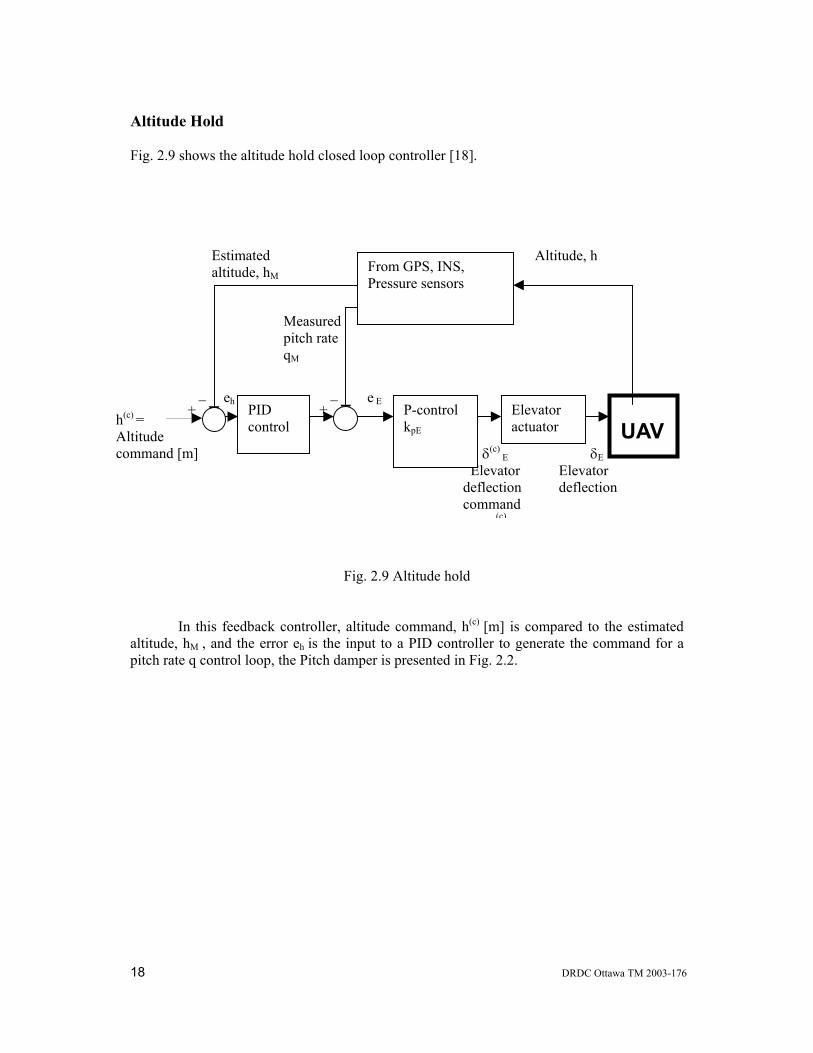
Altitude Hold Fig. 2.9 shows the altitude hold closed loop controller [18].
Fig. 2.9 Altitude hold
In this feedback controller, altitude command, h(c) [m] is compared to the estimated altitude, hM , and the error eh is the input to a PID controller to generate the command for a pitch rate q control loop, the Pitch damper is presented in Fig. 2.2.
h(c) = Altitude command [m]
UAVElevator actuator
δE Elevator deflection
From GPS, INS, Pressure sensors
δ(c) E
Elevator deflection command
(c)
PID control
Estimated altitude, hM
_ +
eh
P-control kpE
Measured pitch rate qM
e E
Altitude, h
_ +
DRDC Ottawa TM 2003-176 19
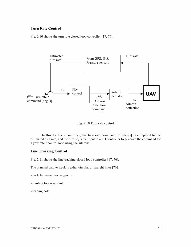
Turn Rate Control Fig. 2.10 shows the turn rate closed loop controller [17, 76].
Fig. 2.10 Turn rate control
In this feedback controller, the turn rate command, t(c) [deg/s] is compared to the estimated turn rate, and the error ea is the input to a PD controller to generate the command for a yaw rate r control loop using the ailerons. Line Tracking Control Fig. 2.11 shows the line tracking closed loop controller [17, 76]. The planned path to track is either circular or straight lines [76]: -circle between two waypoints -pointing to a waypoint -heading hold.
t(c) = Turn rate command [deg /s]
UAVAileron actuator
δA Aileron deflection
From GPS, INS, Pressure sensors
δ(c)A
Aileron deflection command
(c)
Estimated turn rate
_ +
PD-control
e A
Turn rate
20 DRDC Ottawa TM 2003-176
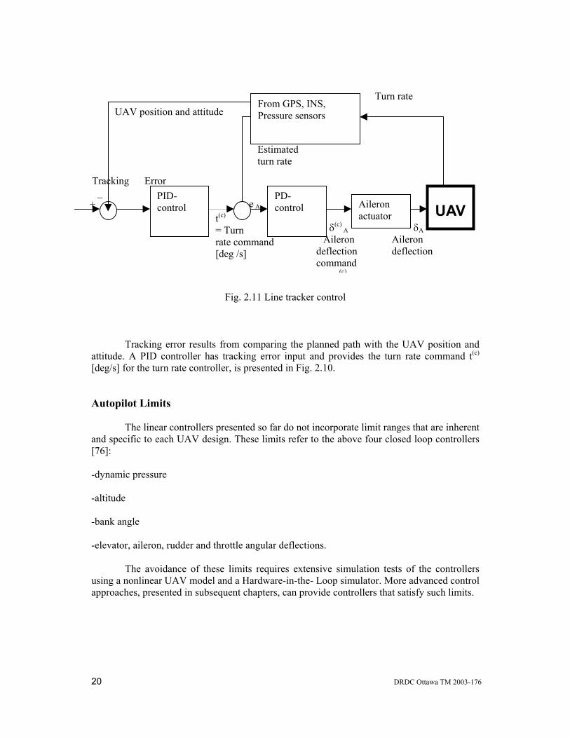
Fig. 2.11 Line tracker control
Tracking error results from comparing the planned path with the UAV position and attitude. A PID controller has tracking error input and provides the turn rate command t(c)
[deg/s] for the turn rate controller, is presented in Fig. 2.10.
Autopilot Limits The linear controllers presented so far do not incorporate limit ranges that are inherent and specific to each UAV design. These limits refer to the above four closed loop controllers [76]: -dynamic pressure -altitude -bank angle -elevator, aileron, rudder and throttle angular deflections. The avoidance of these limits requires extensive simulation tests of the controllers using a nonlinear UAV model and a Hardware-in-the- Loop simulator. More advanced control approaches, presented in subsequent chapters, can provide controllers that satisfy such limits.
t(c)
= Turn rate command [deg /s]
UAVAileron actuator
δA Aileron deflection
From GPS, INS, Pressure sensors
δ(c) A
Aileron deflection command
(c)
Estimated turn rate
Tracking Error _ +
PD-control
e A
Turn rate
PID-control
UAV position and attitude
DRDC Ottawa TM 2003-176 21
Gain Scheduling Controllers Constant gain controllers are not satisfactory for all flight conditions. Improvements in flight performance are obtained using gain scheduling that provides different controller gains for various flight conditions [19].
22 DRDC Ottawa TM 2003-176
3. Comparative Analysis of Flight, Collision Avoidance and Mission Control Approaches for Swarming UAVs
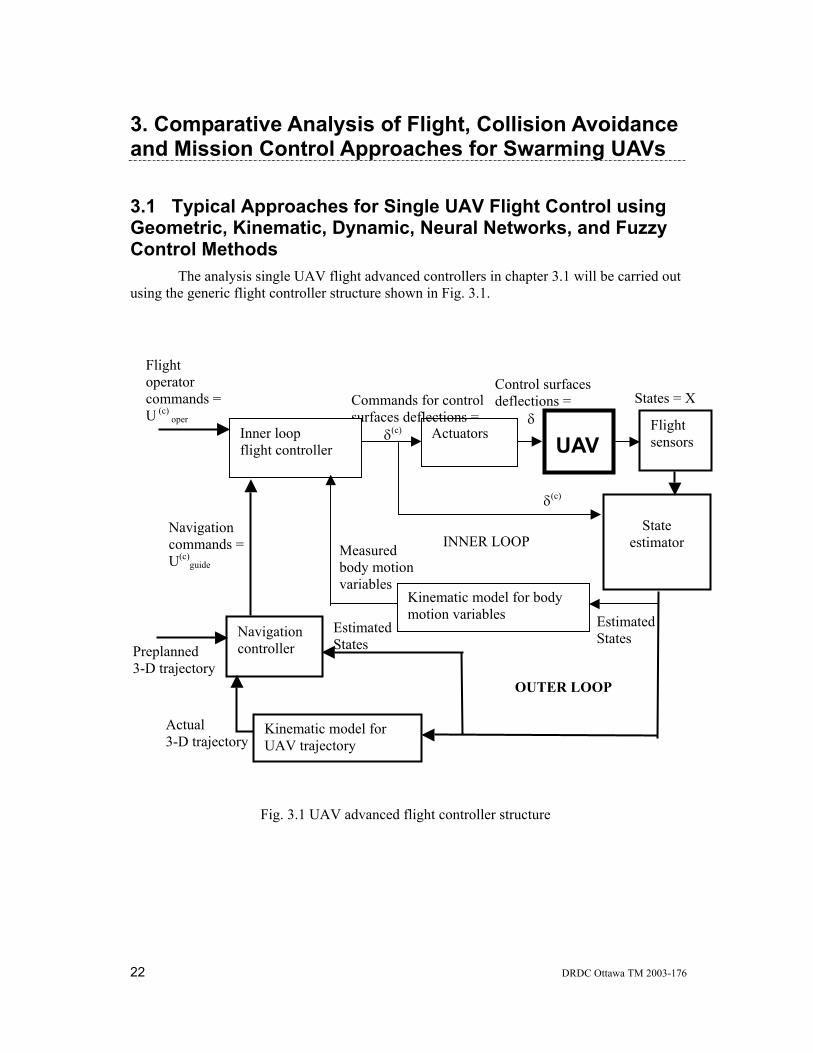
3.1 Typical Approaches for Single UAV Flight Control using Geometric, Kinematic, Dynamic, Neural Networks, and Fuzzy Control Methods The analysis single UAV flight advanced controllers in chapter 3.1 will be carried out using the generic flight controller structure shown in Fig. 3.1.
Fig. 3.1 UAV advanced flight controller structure
UAV
States = X X
INNER LOOP
Actuators
Control surfaces deflections = δ
Kinematic model for body motion variables
Commands for control surfaces deflections = δ(c) Inner loop
flight controller
Measured body motion variables
Flight sensors
State
estimator
OUTER LOOP
Navigation controller Preplanned
3-D trajectory
Navigation commands = U(c)
guide
Flight operator commands = U (c)
oper
Estimated States
δ(c)
Kinematic model for UAV trajectory
Actual 3-D trajectory
Estimated States
DRDC Ottawa TM 2003-176 23
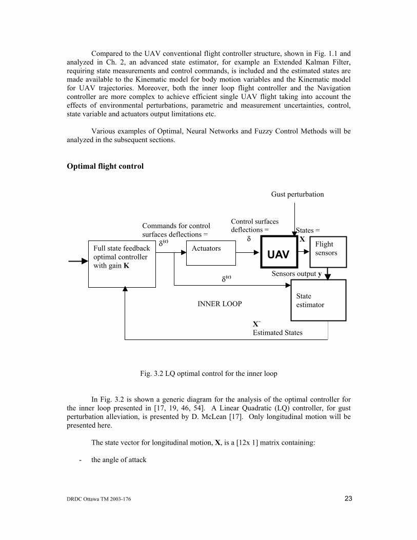
Compared to the UAV conventional flight controller structure, shown in Fig. 1.1 and analyzed in Ch. 2, an advanced state estimator, for example an Extended Kalman Filter, requiring state measurements and control commands, is included and the estimated states are made available to the Kinematic model for body motion variables and the Kinematic model for UAV trajectories. Moreover, both the inner loop flight controller and the Navigation controller are more complex to achieve efficient single UAV flight taking into account the effects of environmental perturbations, parametric and measurement uncertainties, control, state variable and actuators output limitations etc. Various examples of Optimal, Neural Networks and Fuzzy Control Methods will be analyzed in the subsequent sections. Optimal flight control
Fig. 3.2 LQ optimal control for the inner loop In Fig. 3.2 is shown a generic diagram for the analysis of the optimal controller for the inner loop presented in [17, 19, 46, 54]. A Linear Quadratic (LQ) controller, for gust perturbation alleviation, is presented by D. McLean [17]. Only longitudinal motion will be presented here. The state vector for longitudinal motion, X, is a [12x 1] matrix containing:
- the angle of attack
UAV
States = X
INNER LOOP
Actuators
Control surfaces deflections = δ
Commands for control surfaces deflections = δ(c)
Full state feedback optimal controller with gain K
Flight sensors
State estimator
X~ Estimated States
δ(c)
Gust perturbation
Sensors output y
24 DRDC Ottawa TM 2003-176
- pitch rate - vertical displacements of the first five bending modes and their derivatives.
The control vector is given by a u = δ(c) [2 x 1]
- elevator deflection - horizontal canard deflection.
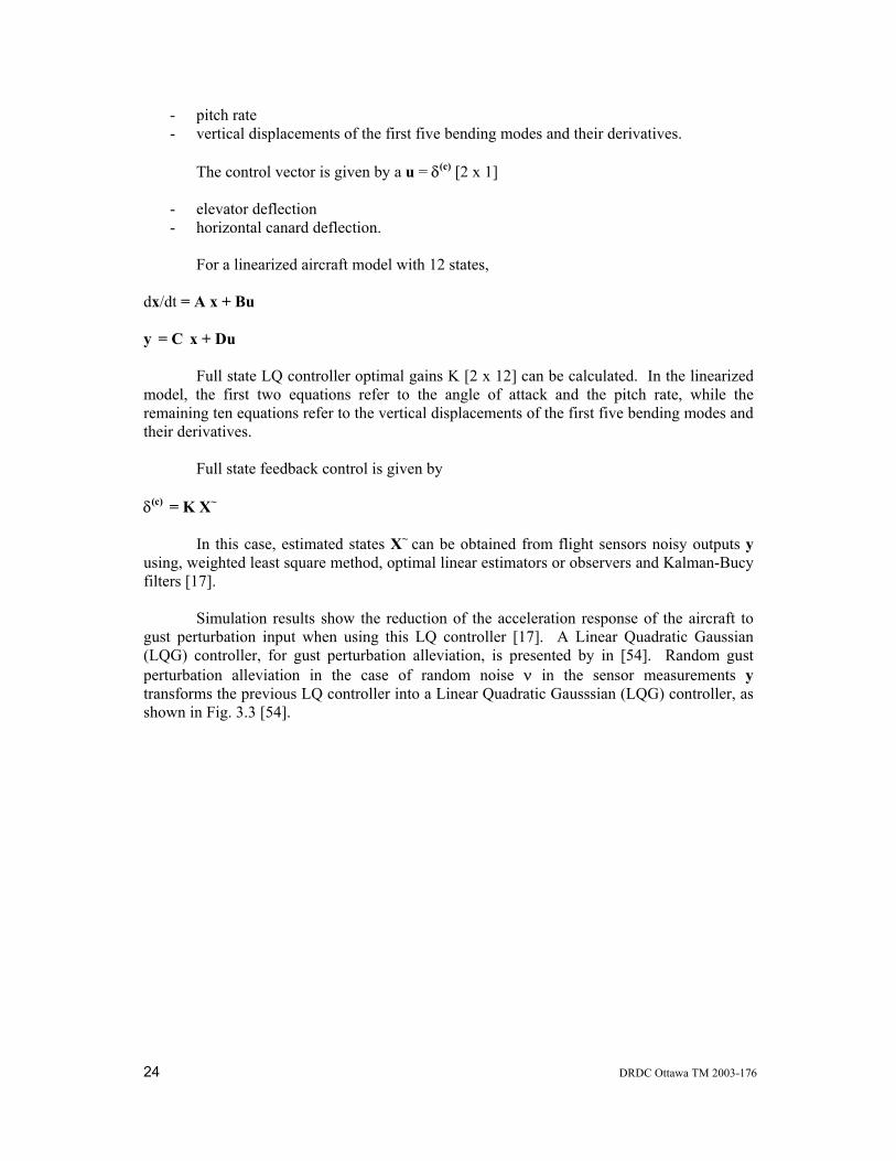
For a linearized aircraft model with 12 states, dx/dt = A x + Bu y = C x + Du Full state LQ controller optimal gains K [2 x 12] can be calculated. In the linearized model, the first two equations refer to the angle of attack and the pitch rate, while the remaining ten equations refer to the vertical displacements of the first five bending modes and their derivatives. Full state feedback control is given by δ(c) = K X~ In this case, estimated states X~ can be obtained from flight sensors noisy outputs y using, weighted least square method, optimal linear estimators or observers and Kalman-Bucy filters [17]. Simulation results show the reduction of the acceleration response of the aircraft to gust perturbation input when using this LQ controller [17]. A Linear Quadratic Gaussian (LQG) controller, for gust perturbation alleviation, is presented by in [54]. Random gust perturbation alleviation in the case of random noise ν in the sensor measurements y transforms the previous LQ controller into a Linear Quadratic Gausssian (LQG) controller, as shown in Fig. 3.3 [54].
DRDC Ottawa TM 2003-176 25
Fig. 3.3 LQG optimal controller for the inner loop
The design of the LQG controller is based on the linearized aircraft model for longitudinal dynamics with the 12 states presented above, augmented with additive terms accounting for the random gust perturbation Ew and random noise ν [2 x 1] in sensor measurements [54] dx/dt = A x + Bu + Ew y = C x + Du + ν The model for the random gust w is obtained from white noise by filtering in accordance with the power spectrum density of the gust perturbation input. Gusts are assumed applied in three different body stations. The Kalman filter gain matrix KK is calculated using the above linear model of the aircraft. Simulation results show a significant reduction of the vertical acceleration response of the aircraft to gust perturbation input when using this LQ controller [54]. Linear quadratic controllers ignore control constraints, for example actuator limits and deflection rate limits for the control surfaces [19]. A feasible control law that accounts for constraints might require a nonlinear controller, but real-time implementation requirements might be in conflict with the computation time in the case that numerous iterations might be required for obtaining a numerical solution. A compromise is possible in a two step controller design approach, see Ch. 75 in [19]
- first step, LQ solution - second step, linear programming (LP) formulation accounting for actuator saturation
limits.
UAV
States = X
INNER LOOP
Actuators
Control surfaces deflections = δ
Commands for control surfaces deflections = δ(c)
Full state feedback optimal controller with gain K
Flight sensors
Kalman filter
X~ Estimated States
δ(c)
Random gust perturbation w
Sensors output y
Random Noise ν
Gain matrix KK
i
26 DRDC Ottawa TM 2003-176
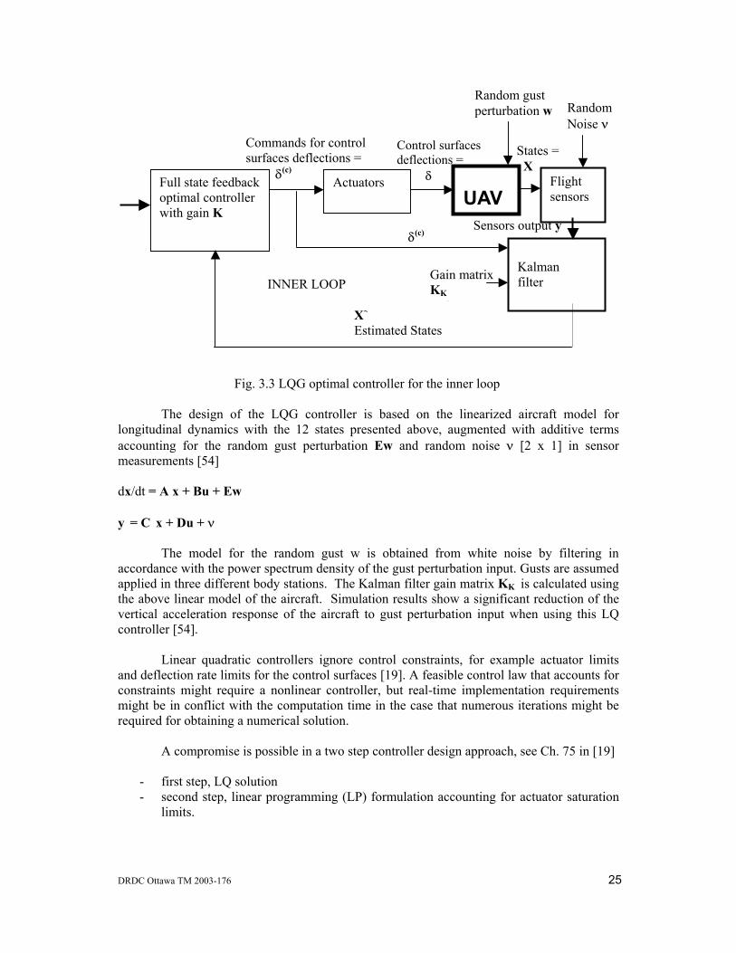
In the case that there is no LP feasible solution, the LQ problem is reformulated for less restrictive penalty parameters for the optimization criterion until a feasible solution results. Robustness of the optimal controllers is highly dependent on the uncertainty of model parameters, in particular the control derivatives. The uncertainty can be accounted for by assuming errors ∆A and ∆B for the matrices A and B of the linearized model used for LQ controller design. These errors have an effect on the closed loop poles in the root locus plot, and obviously, the displacement of any pole on the right hand side of the root locus indicates system instability [46]. Neural Control A Neural Networks (NN) approach is frequently considered for system modeling and control when system dynamics is not completely known or it is not possible to model it analytically for simulations and real time control implementation. NN approach requires first a large set of data linking a rich variety of inputs and corresponding outputs versus time. This set of data can be used to train a NN consisting of layers of nodes that calculate a weighted sum and inputs and rescales nonlinearly the result of the sum into a {-1 to 1} or {0 to 1} real number domain. Training results are a set of values for the weights of the sums that minimize a chosen criterion, for example square root sum of squared differences between set of data output values and the NN outputs for the same inputs [30, 79]. Efficient controller design requires a suitable system model and, in the case of systems that do not have proper analytical models, NN models represent an attractive alternative. Moreover, model based control can be difficult to implement when real time constraints make it impossible to solve numerically the analytical model within each computation cycle time. Again, NN approach is an attractive alternative, given that calculating the output of NN is normally not computationally time consuming. UAV flight control and collision avoidance require often model based controllers and, for this reason NN approach is of particular interest. Fig. 3.4 shows a generic block diagram of a controller using Neural Networks.
Fig. 3.4 Generic block diagram of a controller using Neural Networks (NN)
System
Output= y
Feedforward controller based on NN model of inverse dynamics
+ _
Feedback controller Reference =
r(t)
NN model of inverse dynamics
+ +
System commands= U(c)
Feedback Commands = u(c)
System commands=Uff
(c)
System commands= Ufb
(c)
DRDC Ottawa TM 2003-176 27
In this block diagram, the feedforward controller uses a NN model based inverse dynamics that gives the system commands Uff
(c) for the reference input r(t) [82]. In the feedback control loop, another NN model of the inverse dynamics gives system commands Ufb
(c) for the feedback controller commands u(c) . In this configuration, feedforward controller uses a NN model based inverse dynamics providing basic commands for the system such that system output x(t) tracks closely the reference r(t). Modeling errors and perturbations result in errors r(t) – y(t), and a feedback loop controller is used to regulate the system. The design of the feedback controller for a nonlinear system is facilitated by the inclusion in the feedback control loop of the other NN model of the inverse dynamics that has the purpose to linearize the overall system as seen by the feedback controller. This approach was applied to helicopter flight control [82]. This is only a generic configuration and variations of this block diagram are found in various NN based control schemes. Fig. 3.5 shows a traffic flow controller using Neural Networks.
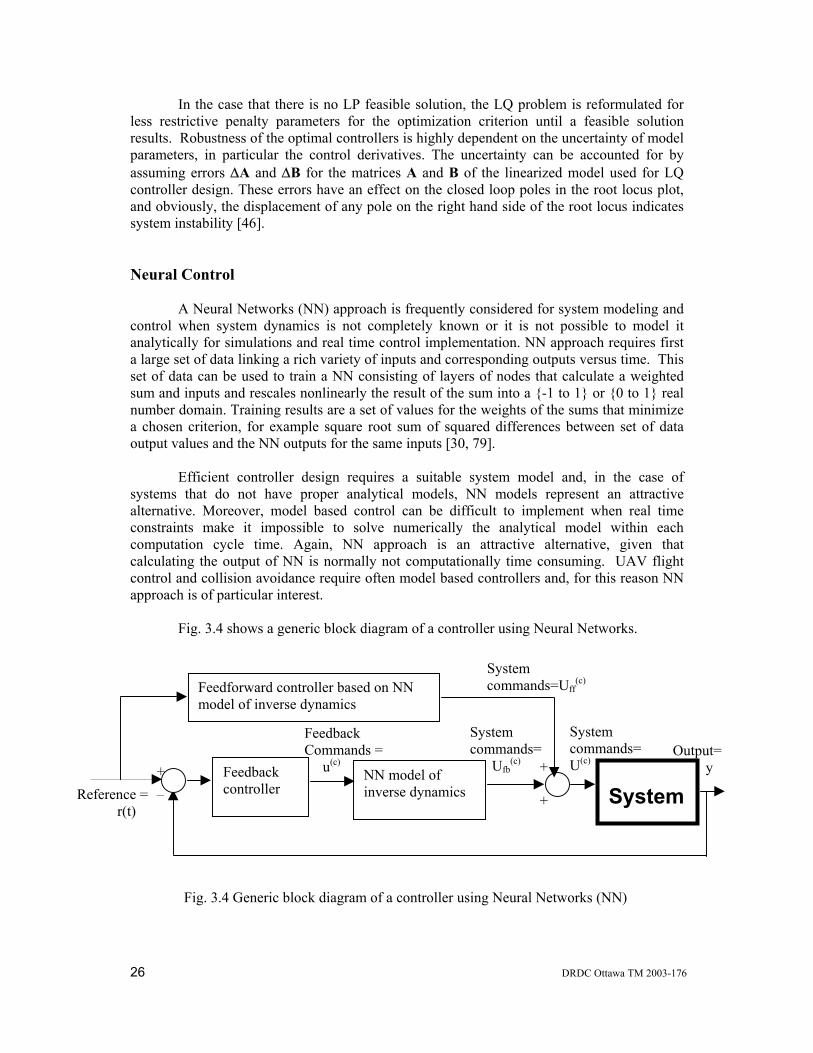
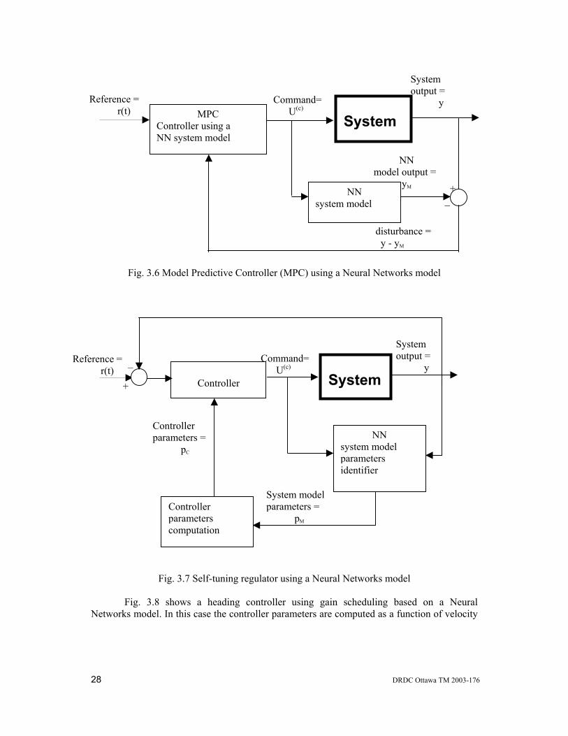
Fig. 3.5 Traffic flow controller using Neural Networks Traffic control is based on the speed commands to the vehicles computed such that the actual traffic density will be close to the desired traffic density [81]. Fig. 3.6 shows a Model Predictive Controller (MPC) using a Neural Networks model. Model Predictive Controller in this case uses a NN system model. The inputs to the MPC controller are the reference r(t) and the disturbance y - yM , calculated using the system output y and the NN system model output yM [80]. Fig. 3.7 shows a self-tuning regulator using a Neural Networks model. NN system model parameters identifier uses as inputs the command U(c) and system output y and provides as output system model parameters pM . These parameters are used to compute the corresponding controller parameters pC . This approach achieves self-regulation of the feedback controller in accordance with the changes in system output y [79].
System
Actual traffic density = y +
_
Desired traffic density = r(t) NN
based controller
Vehicles speed commands= U(c)
Traffic density error = e(t)
28 DRDC Ottawa TM 2003-176
Fig. 3.6 Model Predictive Controller (MPC) using a Neural Networks model
Fig. 3.7 Self-tuning regulator using a Neural Networks model
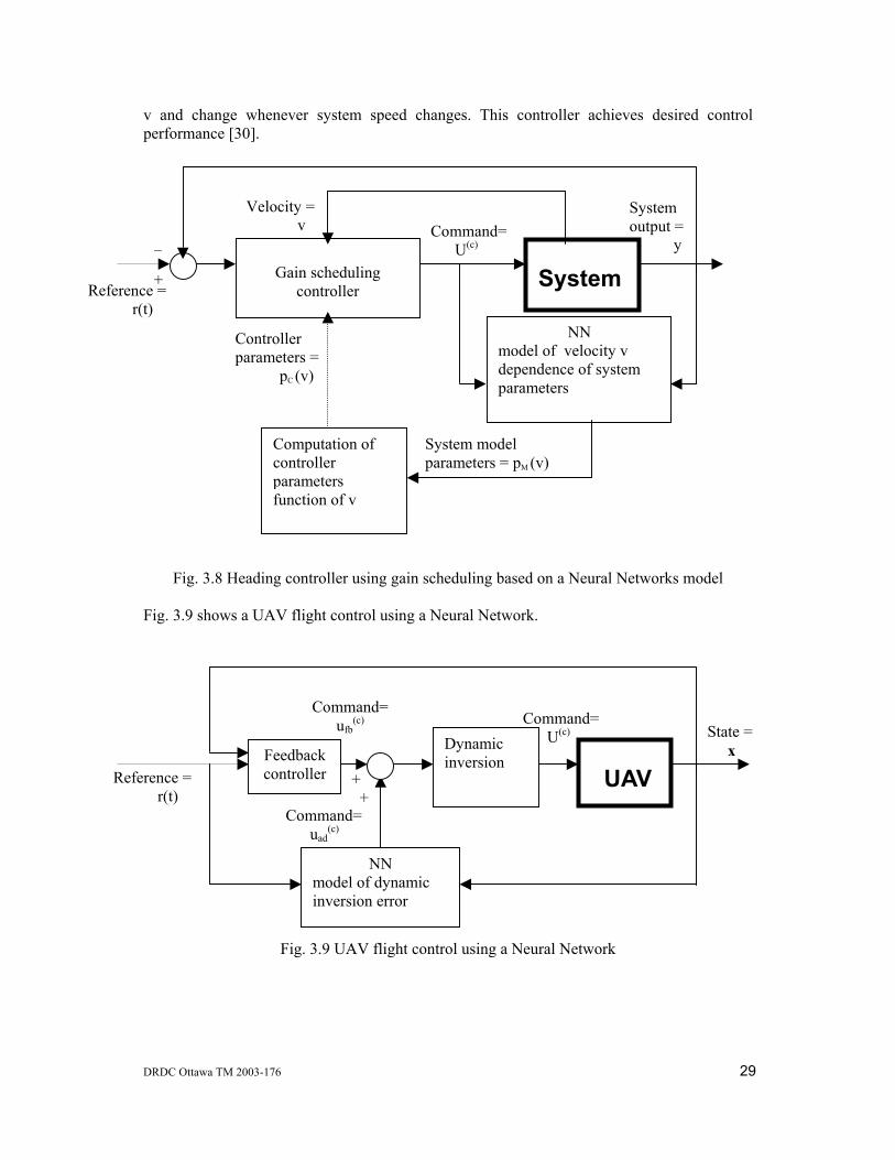
Fig. 3.8 shows a heading controller using gain scheduling based on a Neural Networks model. In this case the controller parameters are computed as a function of velocity
System
System output = y
MPC Controller using a NN system model
Reference = r(t)
NN system model
Command= U(c)
NN model output = yM +
_
disturbance = y - yM
System
System output = y
Controller
Reference = r(t)
NN system model parameters identifier
Command= U(c)
System model parameters = pM
Controller parameters computation
Controller parameters = pC
_ +
DRDC Ottawa TM 2003-176 29
v and change whenever system speed changes. This controller achieves desired control performance [30].
Fig. 3.8 Heading controller using gain scheduling based on a Neural Networks model
Fig. 3.9 shows a UAV flight control using a Neural Network.
Fig. 3.9 UAV flight control using a Neural Network
System
System output = y
Gain scheduling controller Reference =
r(t) NN
model of velocity v dependence of system parameters
Command= U(c)
System model parameters = pM (v)
Computation of controller parameters function of v
Controller parameters = pC (v)
_ +
Velocity = v
UAV
State = x Feedback
controller Reference = r(t)
NN model of dynamic inversion error
+ +
Command= U(c) Dynamic
inversion
Command= ufb
(c)
Command= uad
(c)
30 DRDC Ottawa TM 2003-176
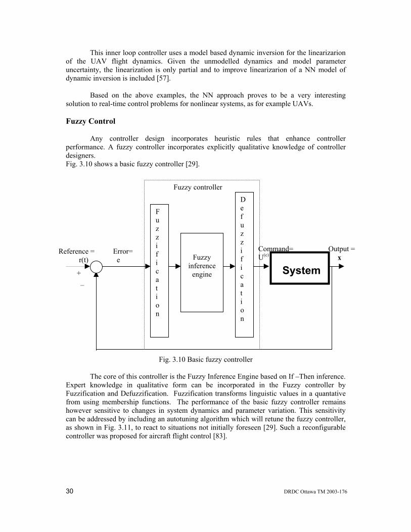
This inner loop controller uses a model based dynamic inversion for the linearizarion of the UAV flight dynamics. Given the unmodelled dynamics and model parameter uncertainty, the linearization is only partial and to improve linearizarion of a NN model of dynamic inversion is included [57]. Based on the above examples, the NN approach proves to be a very interesting solution to real-time control problems for nonlinear systems, as for example UAVs. Fuzzy Control Any controller design incorporates heuristic rules that enhance controller performance. A fuzzy controller incorporates explicitly qualitative knowledge of controller designers. Fig. 3.10 shows a basic fuzzy controller [29].
Fig. 3.10 Basic fuzzy controller
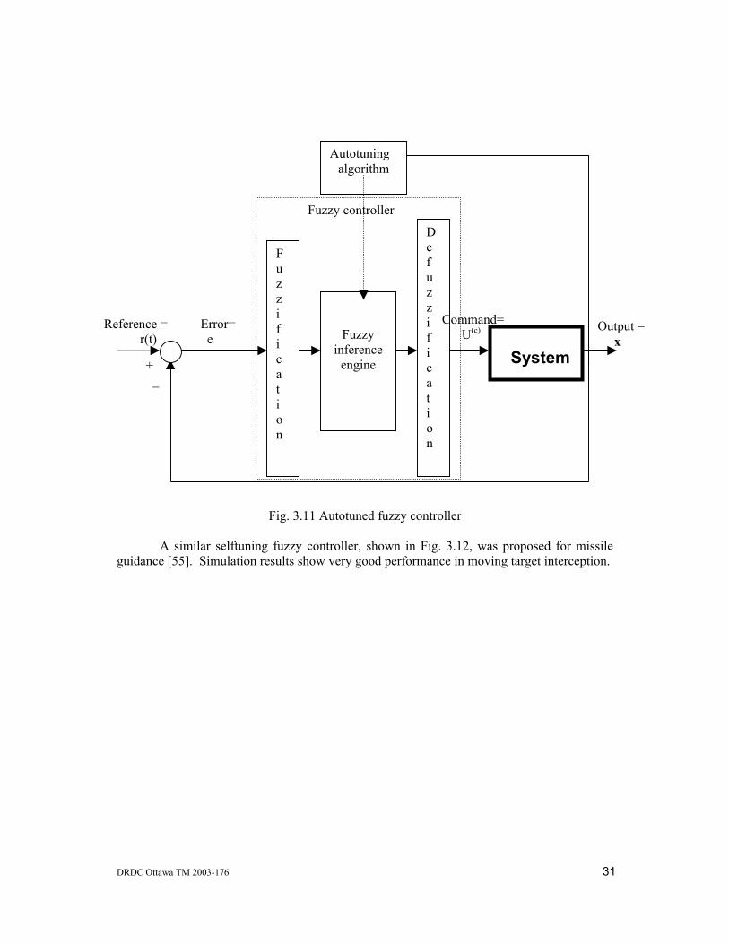
The core of this controller is the Fuzzy Inference Engine based on If –Then inference. Expert knowledge in qualitative form can be incorporated in the Fuzzy controller by Fuzzification and Defuzzification. Fuzzification transforms linguistic values in a quantative from using membership functions. The performance of the basic fuzzy controller remains however sensitive to changes in system dynamics and parameter variation. This sensitivity can be addressed by including an autotuning algorithm which will retune the fuzzy controller, as shown in Fig. 3.11, to react to situations not initially foreseen [29]. Such a reconfigurable controller was proposed for aircraft flight control [83].
System
Output = x
Fuzzy inference
engine
Reference = r(t)
De f u z z i f i c a t i o n
+ _
Command= U(c)
Error= e
F u z z i f i c a t i o n
Fuzzy controller
DRDC Ottawa TM 2003-176 31
Fig. 3.11 Autotuned fuzzy controller
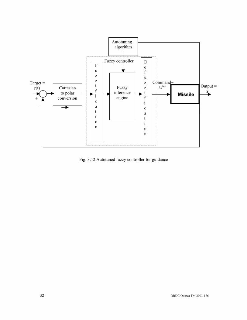
A similar selftuning fuzzy controller, shown in Fig. 3.12, was proposed for missile guidance [55]. Simulation results show very good performance in moving target interception.
System
Output = x
Fuzzy inference
engine
Reference = r(t)
De f u z z i f i c a t i o n
+ _
Command= U(c)
Error= e
F u z z i f i c a t i o n
Fuzzy controller
Autotuning algorithm
32 DRDC Ottawa TM 2003-176
Fig. 3.12 Autotuned fuzzy controller for guidance
Missile Output = x
Fuzzy inference
engine
Target = r(t)
De f u z z i f i c a t i o n
+ _
Command= U(c)
F u z z i f i c a t i o n
Fuzzy controller
Autotuning algorithm
Cartesian to polar
conversion
DRDC Ottawa TM 2003-176 33
3.2 Swarming UAV Approaches for Path Planning with Collision Avoidance with Fixed Obstacles Approaches for path planning and collision avoidance for swarming UAVs depend on swarming modality and the type of obstacles required to be taken into account. The following typical types are of major interest:
• Fixed obstacles, known at path planning stage; • Fixed obstacles, identified during flight; • Moving aerial vehicles or obstacles known before flight; • Moving obstacles, identified during flight;
This section will analyze the first two types, referring to fixed obstacles. And next section will analyze the last two types, referring to moving obstacles. Path Planning for Collision Avoidance with Fixed Obstacles, Known at Path Planning Stage Numerous papers, authored by Dr. Van Dyke Parunak and collaborators, proposed the use of digital pheromones for swarming UAV guidance and collision avoidance [70-74]. The approach proposed in these papers is inspired by biological swarming coordination solutions, in particular from the coordinated activities of ants and other insects, based on sensing and depositing pheromones, i.e. chemical scent markers. In order to imitate this strategy, digital pheromones are proposed for swarming UAV guidance and collision avoidance. These digital pheromones are computer generated markers intended to guide the UAVs in an environment with obstacles. Dr. Eric Bonabeau made a relevant comment regarding the fact that several human operators are presently needed to control a single UAV and we would like to have several, if not thousands of micro UAVs controlled by one operator [72]. The proposed solution for generating digital pheromones is the artificial potential field approach from robotics [52]. Obstacles in robotic workspace are artificially assumed surrounded by repulsive potential fields, similar to same polarity electric field. In this electric field case, objects charged with the same polarity are subject to physically generated repulsive forces and this permits avoidance of moving object collisions. In the case of moving robot arms or mobile robots, the potential fields are artificial and obviously do not generate repulsive forces for collision avoidance. In the robotics case, the collision with obstacles is avoided using robot actuators under model based control. A dynamic model in operational space of the robot includes not only physical forces and torques acting on the arm (gravity, actuators torques, Coriolis forces, drag forces etc) but also repulsive forces assumed artificially as acting on the robot structure. The operational space dynamic model plus a kinematic model between operational space and actuator space permit one to apply commands to the actuators such that not only physical forces and torques are realized, but the artificial potential field is also realized to simulate repulsive forces between the robot and the obstacles. The nonlinear dependence between the proposed artificial potential fields and their realization using robot actuators has to be taken into account in the vehicle motion control and results in a dynamic model based robot controller. Besides this, the construction of artificial potential fields for planning robot paths in an environment with obstacles, is another complex task [52]. The construction of artificial
34 DRDC Ottawa TM 2003-176
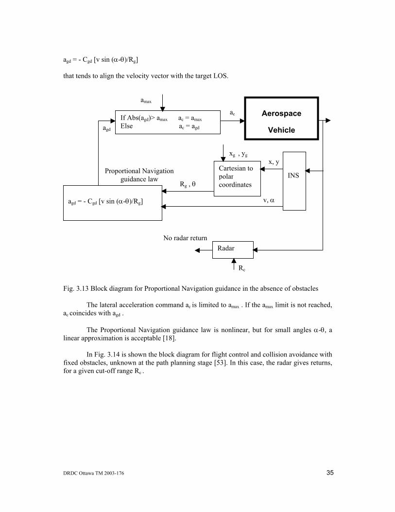
potential fields is different for the case of fixed and moving obstacles. Reference [52], used by Dr. Van Dyke Parunak and collaborators for the creation of digital pheromones, was developed for stationary obstacles (I quote from page 515, “our naive assumptions-stationary obstacles, fixed destination, perfect information, ideal sensors and ideal bounded-torque actuators, are themselves unrealistic, and their relaxation is imperative in the long run”). These assumptions permitted, however, the construction of artificial potential fields for an environment with complex fixed obstacles. There are other publications presenting artificial potential fields for moving obstacles, but only for simple and very limited number of obstacles. Moreover, the real time robot control with avoidance of collision with moving obstacles using artificial potential fields is computationally very demanding and requires exact feedback linearization of the robot nonlinear dynamics [39, 40]. Dr. Van Dyke Parunak and collaborators assumed however that the artificial potential field approach presented in reference [52] is applicable also for moving obstacles, in particular for swarming UAVs. This assumption requires further analysis and extensive theoretical development to lead to a applicable solution. This issue will be further analysed in Ch. 4. In the form published up to this time, the approach proposed by Dr. Van Dyke Parunak and collaborators is applicable only for path planning in the presence of known fixed obstacles and cannot be applied to swarming UAVs unless it is developed further. Similarly, in reference [69], solutions are presented to group behaviour control for a robotic team for providing high level commands for military behaviours as, for example: assault a position, formation moves or other group movements. This permits one to address issues regarding requirements for communications, terrain reasoning, reasoning under uncertainty and missions for teams with large numbers of robots (up to several thousand). Lower level commands for collision avoidance, slippage avoidance, waypoint choice are left for technical solutions to be developed elsewhere. The split between high-level team strategy and low-level vehicle control results, however, in solutions which are not practical either at the strategic level or at the technical level. Several other contributions presented later will encompass a larger view covering, at least partly, both strategic and technical aspects. Path Planning for Collision Avoidance with Fixed Obstacles, Unknown at Path Planning Stage An interesting solution for guidance strategy and collision avoidance with fixed obstacles, not known at the path planning stage, is proposed in [53]. For the convenience of the analysis, this solution will be presented first for guidance in absence of obstacles (Fig. 3.13) and then for the obstacle collision avoidance case (Fig. 4.14). In Fig. 3.13 is shown the block diagram for Proportional Navigation guidance in the absence of obstacles [18, 53]. In this case, the radar gives no return for a given cut-off range Rc . The Inertial Navigation System (INS) provides vehicle current position (x, y) velocity amplitude and angle (v, α) in an inertial reference system. Given the target position xg , yg , a Cartesian to polar coordinates transformation gives the target polar coordinates Rg , θ relative to the vehicle. The difference α-θ is a guidance system error to be reduced to zero by control such that the velocity vector direction will coincide with target Line Of Sight (LOS). Proportional Navigation guidance law [18, 53], provides a lateral acceleration
DRDC Ottawa TM 2003-176 35
agd = - Cgd [v sin (α-θ)/Rg] that tends to align the velocity vector with the target LOS. Fig. 3.13 Block diagram for Proportional Navigation guidance in the absence of obstacles The lateral acceleration command ac is limited to amax . If the amax limit is not reached, ac coincides with agd . The Proportional Navigation guidance law is nonlinear, but for small angles α-θ, a linear approximation is acceptable [18]. In Fig. 3.14 is shown the block diagram for flight control and collision avoidance with fixed obstacles, unknown at the path planning stage [53]. In this case, the radar gives returns, for a given cut-off range Rc .
x, y
ac
INS
If Abs(agd)> amax ac = amax Else ac = agd
Proportional Navigation guidance law
agd
Aerospace
Vehicle
Cartesian to polar coordinates
agd = - Cgd [v sin (α-θ)/Rg] v, α
Rg , θ
amax
Radar No radar return
Rc
xg , yg
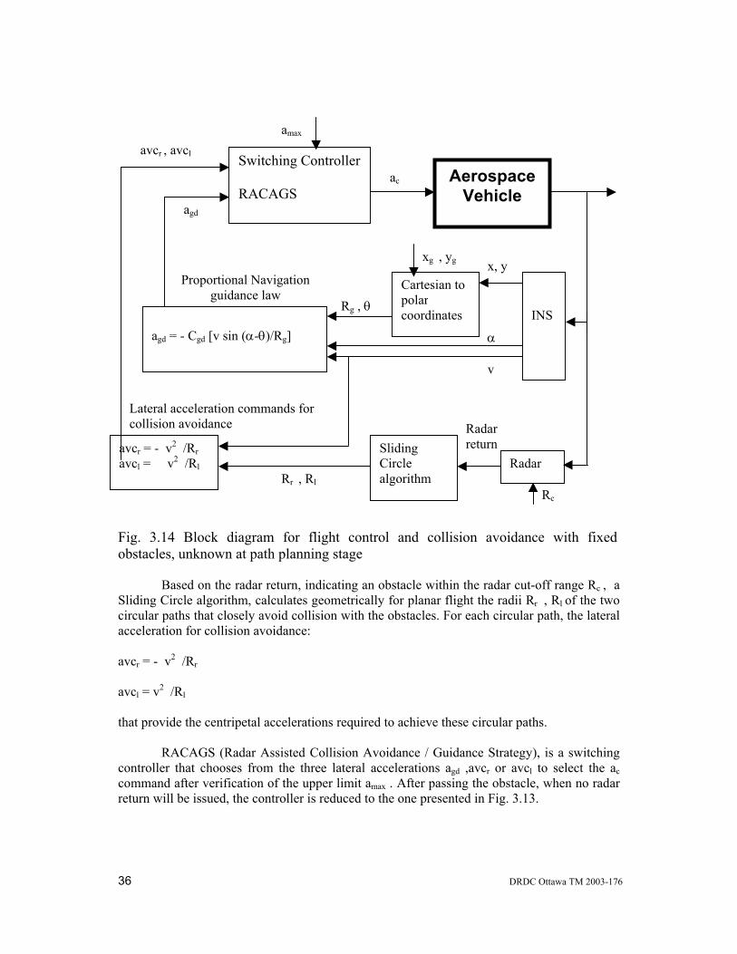
36 DRDC Ottawa TM 2003-176
Fig. 3.14 Block diagram for flight control and collision avoidance with fixed obstacles, unknown at path planning stage Based on the radar return, indicating an obstacle within the radar cut-off range Rc , a Sliding Circle algorithm, calculates geometrically for planar flight the radii Rr , Rl of the two circular paths that closely avoid collision with the obstacles. For each circular path, the lateral acceleration for collision avoidance: avcr = - v2 /Rr avcl = v2 /Rl that provide the centripetal accelerations required to achieve these circular paths. RACAGS (Radar Assisted Collision Avoidance / Guidance Strategy), is a switching controller that chooses from the three lateral accelerations agd ,avcr or avcl to select the ac command after verification of the upper limit amax . After passing the obstacle, when no radar return will be issued, the controller is reduced to the one presented in Fig. 3.13.
x, y
ac
INS
Switching Controller
RACAGS
Proportional Navigation guidance law
agd
Cartesian to polar coordinates
agd = - Cgd [v sin (α-θ)/Rg] α
Rg , θ
amax
Radar
Radar return
Rc
xg , yg
Sliding Circle algorithm Rr , Rl
avcr = - v2 /Rr avcl = v2 /Rl
avcr , avcl
Lateral acceleration commands for collision avoidance
v
Aerospace Vehicle
DRDC Ottawa TM 2003-176 37
This approach is further developed to account for obstacles larger than the radar detection cone, multiple fixed obstacles and for the 3-D case for obstacle avoidance when flying over the obstacle might be preferable to bypassing it in a horizontal circular flight path. This approach is technically more developed than the ones presented so far in this section, but still limits the representation of the aerospace vehicle to a point mass. For collision avoidance, similar to the approach used in robotics, vehicle geometric dimensions are added to the virtual circle surrounding the obstacle. Moreover, the lateral accelerations agd , avcr or avcl are assumed realizable as such, i.e. vehicle dynamics and actuator saturation or control surfaces constraints are ignored not only during the controller design, but also for simulations. An integrated simulation environment for Multi-UAV flight toward fixed targets with collision avoidance for fixed obstacles was developed using MATHWORKS tools [61]. MATHWOKS tools needed for this simulator are:
• MATLAB and Simulink; • Stateflow; • Virtual Reality Toolbox; • DSP Blockset.
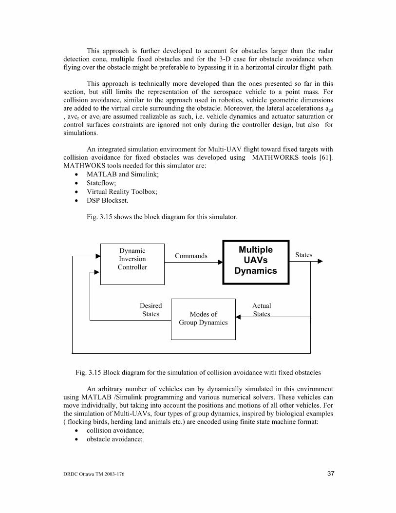
Fig. 3.15 shows the block diagram for this simulator.
Fig. 3.15 Block diagram for the simulation of collision avoidance with fixed obstacles An arbitrary number of vehicles can by dynamically simulated in this environment using MATLAB /Simulink programming and various numerical solvers. These vehicles can move individually, but taking into account the positions and motions of all other vehicles. For the simulation of Multi-UAVs, four types of group dynamics, inspired by biological examples ( flocking birds, herding land animals etc.) are encoded using finite state machine format:
• collision avoidance; • obstacle avoidance;
Multiple UAVs
Dynamics
Modes of
Group Dynamics
States
Actual States
Desired States
Dynamic Inversion Controller
Commands
38 DRDC Ottawa TM 2003-176
• target acquisition; • formation keeping.
The current mode of group dynamics is selected based on the actual states of the group of vehicles. A Dynamic Inversion Controller provides commands to the vehicle for the currently active mode of group dynamics. The fixed targets and obstacles can be changed during the simulation by providing their position and radii. The blocks of this simulator are not sufficiently documented in this publication for a critical analysis. MATHWORKS offers however an Aerospace Blockset for propulsion, control systems, system dynamics and actuators for autopilot and guidance system design and closed loop modeling for aircraft.
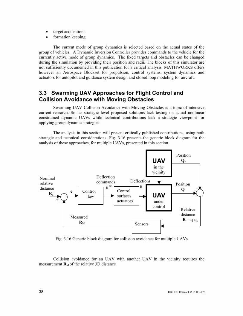
3.3 Swarming UAV Approaches for Flight Control and Collision Avoidance with Moving Obstacles Swarming UAV Collision Avoidance with Moving Obstacles is a topic of intensive current research. So far strategic level proposed solutions lack testing on actual nonlinear constrained dynamic UAVs while technical contributions lack a strategic viewpoint for applying group dynamic strategies The analysis in this section will present critically published contributions, using both strategic and technical considerations. Fig. 3.16 presents the generic block diagram for the analysis of these approaches, for multiple UAVs, presented in this section.
Fig. 3.16 Generic block diagram for collision avoidance for multiple UAVs Collision avoidance for an UAV with another UAV in the vicinity requires the measurement RM of the relative 3D distance
UAVunder
control Relative distance R = q-qv
Control surfaces actuators
Deflections δ
Sensors
Deflection commands δ
(c)
Control law
Measured RM
Nominal relative distance
Rd
+_
e
UAVin the
vicinity
_ +
Position Q
Position Qv
DRDC Ottawa TM 2003-176 39
R = q-qv where q and qv are the 3D positions of the two UAVs. Multiple UAVs require multiple vectors R. Relative position error is e = Rd - R where Rd is the desired relative 3D distance between UAVs. The resulting commands δ
(c) from the control law are realized by the actuators as actual control surface deflections δ. As a result of δ, the UAV under control changes the q 3D position in such a way as to make R tend toward the desired relative distance Rd and thus maintain flight formation and avoid collision. The sensory and signal processing needs for estimating relative distance R and the design of the control law that provides the commands δ
(c) for control surfaces deflections are very complex processes that are not in a mature enough stage to guarantee swarming UAV flight formation hold and collision avoidance. Contributions analysed in this section solve only each part of the problem and their assembly does not seem to have currently all the components available for robust swarming UAV flight formation hold and collision avoidance. Fig. 3.17 shows a Block diagram for the control of the relative distance between two spacecrafts using a linear control law combined with a nonlinear feedback adaptive compensator [47]. Spacecraft dynamics for filtered tracking error r is obtained from 3-D force equations for two spacecrafts, a leader and a follower, in the leader’s instantaneously coincident (IC) reference frame. In these equations, the 3D force inputs, ul and uf
, are assumed directly realizable, i.e. no dynamic models for actuators and control surface deflections are included and no constraints are considered for the actuator outputs and control surface deflections. As a result, any commands for the force inputs, ul and uf
, are assumed realizable, including the y-components, in the sideway direction of the wings, were no actuator is active. Subtracting corresponding force equations for each of the three coordinates, the relative speed q dynamics equation is obtained. This equation is converted into a dynamic equation for the filtered tracking error r, using r = d/dt (qd – q) + Λ(qd – q) where qd (t) is the desired relative position. It can be a function of time. This conversion is needed for the adaptive algorithm with a 3x3 diagonal gain matrix Γ, used for the estimation θ~ of the parameters and perturbation vector θ = [mf, mf M G, mf /ml , Fd ]T
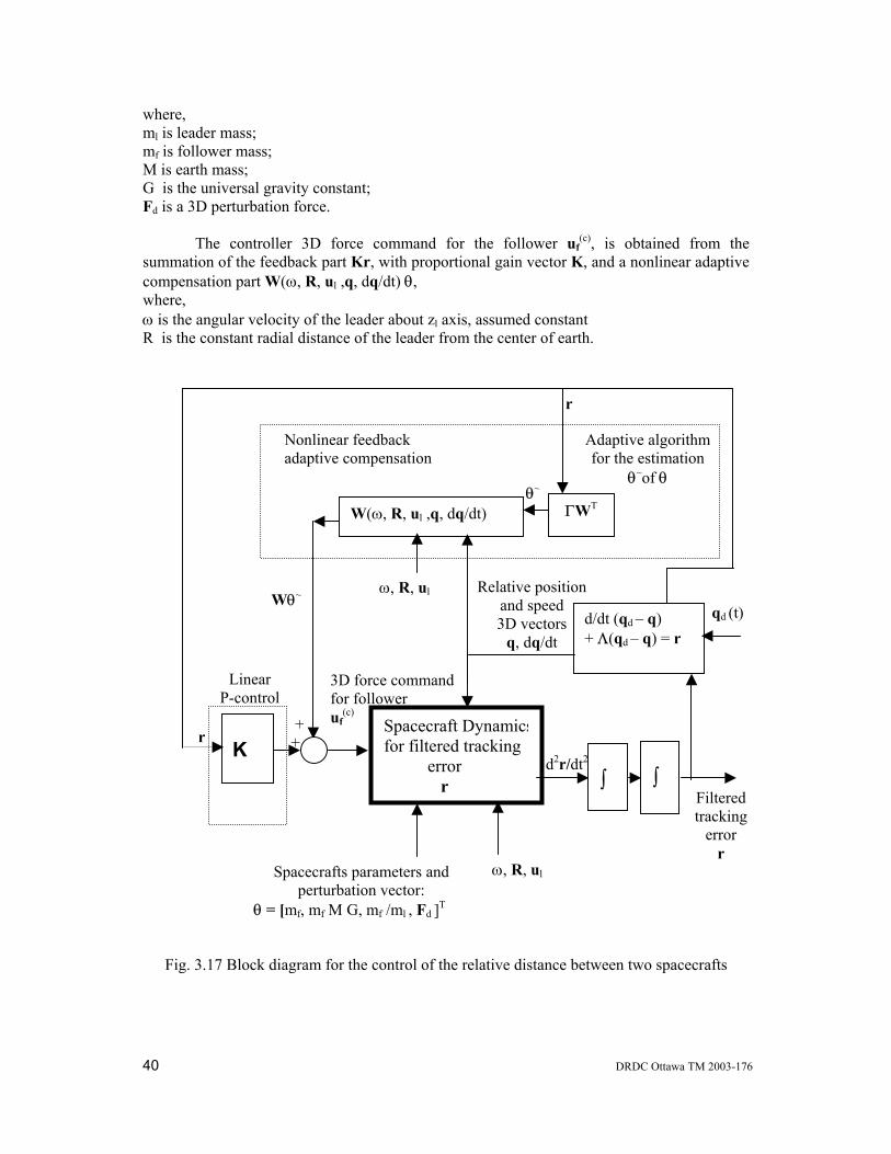
40 DRDC Ottawa TM 2003-176
where, ml is leader mass; mf is follower mass; M is earth mass; G is the universal gravity constant; Fd is a 3D perturbation force. The controller 3D force command for the follower uf
(c), is obtained from the summation of the feedback part Kr, with proportional gain vector K, and a nonlinear adaptive compensation part W(ω, R, ul ,q, dq/dt) θ, where, ω is the angular velocity of the leader about zl axis, assumed constant R is the constant radial distance of the leader from the center of earth.
Fig. 3.17 Block diagram for the control of the relative distance between two spacecrafts
Spacecraft Dynamicsfor filtered tracking error r
d/dt (qd – q) + Λ(qd – q) = r
qd (t)
W(ω, R, ul ,q, dq/dt)
K
ω, R, ul
θ~
r
Spacecrafts parameters and perturbation vector:
θ = [mf, mf M G, mf /ml , Fd ]T
Linear P-control
+ +
Wθ~
ΓWT
d2r/dt2
r
3D force command for follower uf
(c)
∫ ∫ Filtered tracking
error r
Relative position and speed 3D vectors
q, dq/dt
Adaptive algorithm for the estimation
θ~of θ
Nonlinear feedback adaptive compensation
ω, R, ul
DRDC Ottawa TM 2003-176 41
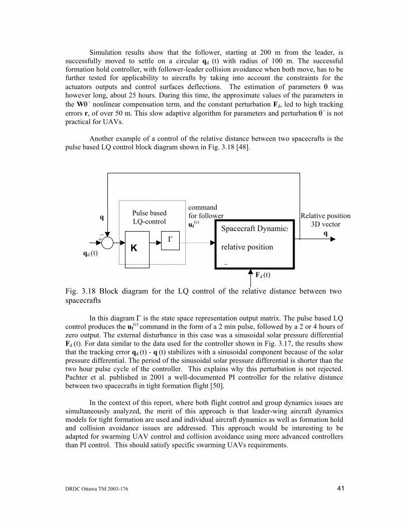
Simulation results show that the follower, starting at 200 m from the leader, is successfully moved to settle on a circular qd (t) with radius of 100 m. The successful formation hold controller, with follower-leader collision avoidance when both move, has to be further tested for applicability to aircrafts by taking into account the constraints for the actuators outputs and control surfaces deflections. The estimation of parameters θ was however long, about 25 hours. During this time, the approximate values of the parameters in the Wθ~ nonlinear compensation term, and the constant perturbation Fd, led to high tracking errors r, of over 50 m. This slow adaptive algorithm for parameters and perturbation θ~ is not practical for UAVs. Another example of a control of the relative distance between two spacecrafts is the pulse based LQ control block diagram shown in Fig. 3.18 [48]. Fig. 3.18 Block diagram for the LQ control of the relative distance between two spacecrafts In this diagram Γ is the state space representation output matrix. The pulse based LQ control produces the uf
(c) command in the form of a 2 min pulse, followed by a 2 or 4 hours of zero output. The external disturbance in this case was a sinusoidal solar pressure differential Fd (t). For data similar to the data used for the controller shown in Fig. 3.17, the results show that the tracking error qd (t) - q (t) stabilizes with a sinusoidal component because of the solar pressure differential. The period of the sinusoidal solar pressure differential is shorter than the two hour pulse cycle of the controller. This explains why this perturbation is not rejected. Pachter et al. published in 2001 a well-documented PI controller for the relative distance between two spacecrafts in tight formation flight [50]. In the context of this report, where both flight control and group dynamics issues are simultaneously analyzed, the merit of this approach is that leader-wing aircraft dynamics models for tight formation are used and individual aircraft dynamics as well as formation hold and collision avoidance issues are addressed. This approach would be interesting to be adapted for swarming UAV control and collision avoidance using more advanced controllers than PI control. This should satisfy specific swarming UAVs requirements.
Spacecraft Dynamics
relative position
qqd (t)
K
q Pulse basedLQ-control
_ + Γ
command for follower uf
(c) Relative position
3D vector q
Fd (t)
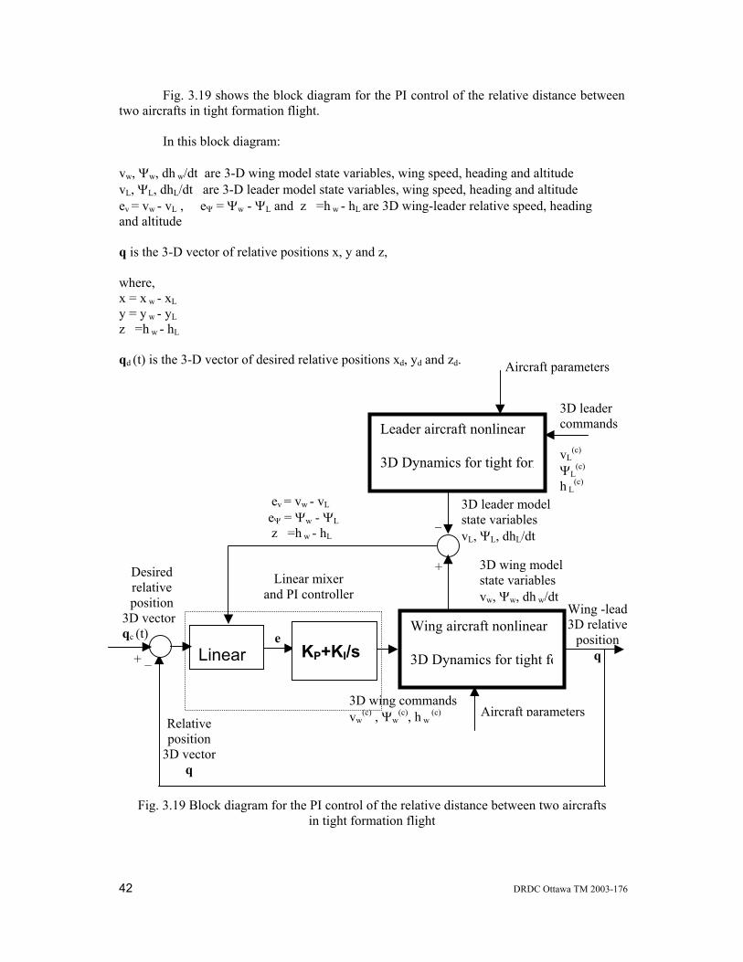
42 DRDC Ottawa TM 2003-176
Fig. 3.19 shows the block diagram for the PI control of the relative distance between two aircrafts in tight formation flight. In this block diagram: vw, Ψw, dh w/dt are 3-D wing model state variables, wing speed, heading and altitude vL, ΨL, dhL/dt are 3-D leader model state variables, wing speed, heading and altitude ev = vw - vL , eΨ = Ψw - ΨL and z =h w - hL are 3D wing-leader relative speed, heading and altitude q is the 3-D vector of relative positions x, y and z, where, x = x w - xL y = y w - yL z =h w - hL qd (t) is the 3-D vector of desired relative positions xd, yd and zd.
Fig. 3.19 Block diagram for the PI control of the relative distance between two aircrafts in tight formation flight
Wing aircraft nonlinear
3D Dynamics for tight fo
Desired relative position
3D vector qc (t) Linear
e
Linear mixer and PI controller
+ _
3D wing commands vw
(c) , Ψw(c), h w
(c)
Wing -lead3D relative
position q
Relative position
3D vector q
Aircraft parameters
KP+KI/s
Leader aircraft nonlinear
3D Dynamics for tight form
Aircraft parameters
3D wing model state variables vw, Ψw, dh w/dt
3D leader model state variables vL, ΨL, dhL/dt
_ +
ev = vw - vL eΨ = Ψw - ΨL z =h w - hL
3D leader commands vL
(c) ΨL
(c) h L
(c)
DRDC Ottawa TM 2003-176 43
e(t)= q(t) - qd (t) is the 3D vector of the longitudinal, lateral and heading errors, with regard to their desired values. vw
(c) , Ψw(c), h w
(c) are the 3D wing commands. Aircraft parameters refer to the parameters of the 3D dynamics models of the leader and the wing aircraft regarding mass and stability derivative coefficients for the speed, heading and altitude equations of the respective speed-hold, heading-hold and altitude hold autopilots [50]. An important contribution of this paper is the calculation of the new corrections for tight formation stability derivatives for the case of the wing flying in the vortex of the leader, within 10% of the lead wingspan, to achieve drag reduction and, consequently significant reduction in fuel consumption and increase in endurance by 30 %. The PI controller was designed using linear perturbation equations obtained by linearizing the leader and wing 3-D nonlinear dynamic equations. Simulation results confirmed the performance of this approach in tight formation hold and collision avoidance in the presence 30-degree lead heading changes. The results for wing-leader collision avoidance are relevant for UAV collision avoidance with a moving obstacle. In Fig. 3.14 from the previous section, was presented an alternative collision avoidance approach, but proposed only for the case of fixed obstacles. A more useful approach for UAV 3-D local trajectory planning with collision avoidance proposed for both fixed and moving obstacles is presented by Sasiadek and Duleba in [51]. Autonomous navigation can be achieved in this case by splitting the motion planning problem into two stages:
• decision mode; • trace mode.
In decision mode, next step attitude and velocity are determined taking into account the distance to the goal, best vehicle orientation and obstacle avoidance. In this mode, however, local optimum can occur in the artificial potential field approach to collision avoidance. As a result the vehicle can be trapped and stopped permanently away from the goal.
In trace mode, the controller is switched to path tracking along the boundary of the obstacle, ultimately tending towards the goal, by temporarily even going away from the goal for exiting from a local optimum. The control commands satisfy constraints regarding maximum and minimum velocity, maximum acceleration, minimum and maximum orientation rate changes and safe distance to the obstacle etc. Simulation results illustrate the operation of the proposed approach in trajectory planning and collision avoidance with fixed and moving obstacles. Cooperative decentralized control schemes for UAVs are presented in [62 – 65]. Operational space for the UAVs is partitioned into quadratic cells where targets and obstacles can reside and in which, at one time, only one UAV can be present. In discrete time representation, an UAV has the choice of moving into another cell, but in only three directions, - 45°, 0° or 45°, to account for maneuverability constraints. The proposed approach focuses on Neural Network learning using Bayesian rules to account for sensor random errors.
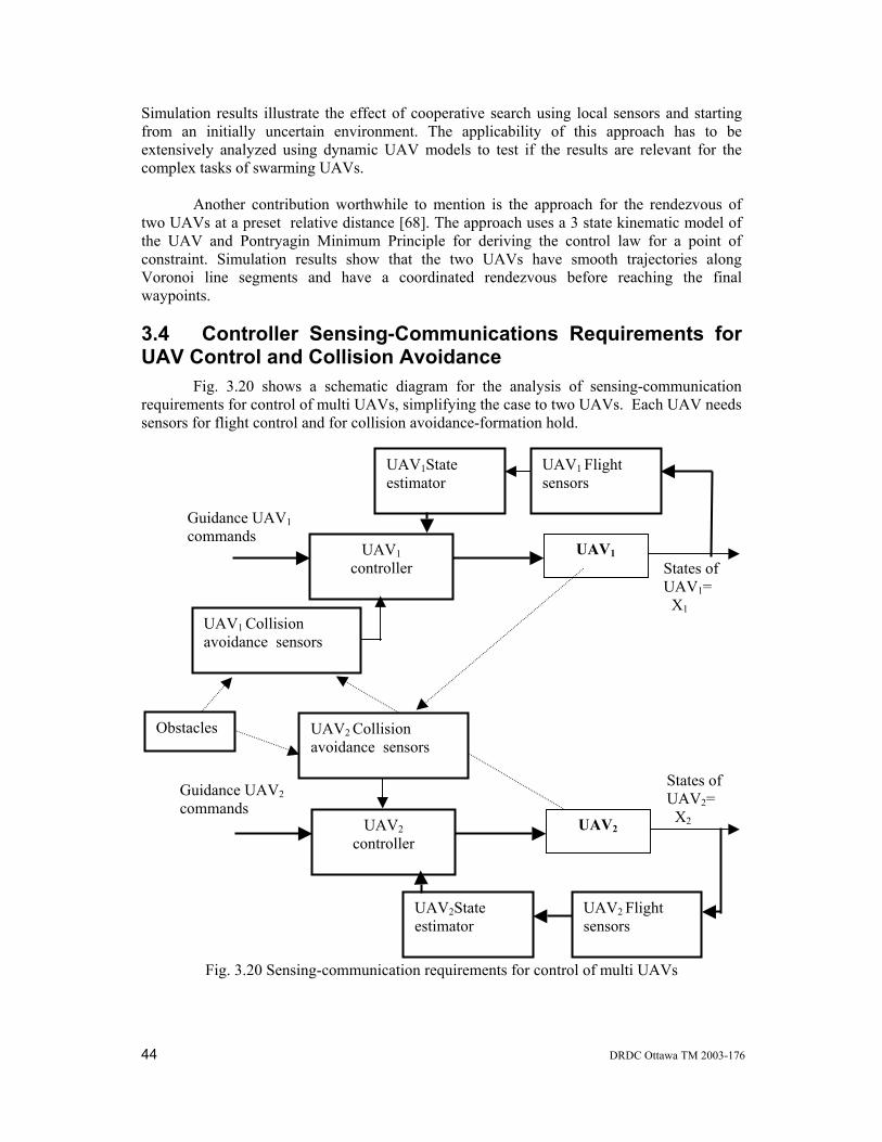
44 DRDC Ottawa TM 2003-176
Simulation results illustrate the effect of cooperative search using local sensors and starting from an initially uncertain environment. The applicability of this approach has to be extensively analyzed using dynamic UAV models to test if the results are relevant for the complex tasks of swarming UAVs. Another contribution worthwhile to mention is the approach for the rendezvous of two UAVs at a preset relative distance [68]. The approach uses a 3 state kinematic model of the UAV and Pontryagin Minimum Principle for deriving the control law for a point of constraint. Simulation results show that the two UAVs have smooth trajectories along Voronoi line segments and have a coordinated rendezvous before reaching the final waypoints.
3.4 Controller Sensing-Communications Requirements for UAV Control and Collision Avoidance Fig. 3.20 shows a schematic diagram for the analysis of sensing-communication requirements for control of multi UAVs, simplifying the case to two UAVs. Each UAV needs sensors for flight control and for collision avoidance-formation hold.
Fig. 3.20 Sensing-communication requirements for control of multi UAVs
States of UAV1= X1
UAV1
UAV1 Flight sensors
UAV1State estimator
UAV1 controller
Guidance UAV1 commands
UAV1 Collision avoidance sensors
States of UAV2= X2 UAV2
UAV2 Flight sensors
UAV2State estimator
UAV2 controller
Guidance UAV2 commands
UAV2 Collision avoidance sensors
Obstacles
DRDC Ottawa TM 2003-176 45
Flight sensors are needed for the inner loop flight controller and include body motion sensors as for example: rate gyros for pitch, yaw and roll, accelerometers etc. A UAV state estimator is usually required to obtain state variable estimations. Collision avoidance-formation hold use range sensors able to measure relative distance to the other UAV, or to obstacles that have to be avoided. An integrated INS/GPS can serve both flight sensing needs and collision avoidance-formation needs. For example, from GPS, INS, pressure sensors, the following quantities can be determined: - ground speed [m/s] - airspeed [m/s] - altitude, longitude, altitude [m] - roll, pitch, yaw rates [deg/s] - body frame accelerations [m/s2 ]
- direction [deg] - dynamic pressure [kPa] - barometric pressure [kPa]. The ground control station sends guidance commands to the UAVs and receives data needed for monitoring. Besides sensing, swarming UAVs have specific communication needs. These needs depend on the approaches chosen for flight control and for collision avoidance-formation hold. Range sensing is based on triangulation methodology using appropriate onboard sensors. Group flight can be organized into two basic structures:
- leader followers structure; - decentralized structure.
Leader-follower structures were used in several papers analyzed in this report, for example in the case of tight formation control [50] and for providing string stability. Decentralized structure is promoted by some group dynamics advocates, for example by E. Bonabeau [72] and Van Dyke Parunak [73-74]. The problems of decentralized control have, however to be addressed, given that string instability can also occur in large decentralized structures.
46 DRDC Ottawa TM 2003-176
4. Advanced UAV Control Design Issues for Swarming UAVs
4.1 Feedback Linearization of UAV Nonlinear Dynamics and Controller Design
Feedback Linearization Approach Nonlinearities of the UAV flight dynamics represent a major difficulty in controller and collision avoidance design. Conventional flight controller design approaches, presented in ch. 2, were all based on a locally linearized aircraft model, for trim conditions. As flight conditions further from trim occur, the performance of the controller degrades. A tempting solution for solving this problem is feedback linearization of UAV nonlinear dynamics, which, in principle, results in a global linearization and permit the design of controllers that have the same performance for all flight conditions. In practice, model based feedback linearization is only partial because of unmodelled dynamics and parameters/states estimation uncertainty. Moreover, some advanced control approaches are well developed particularly for linear systems. Nonlinear systems require linearization for the design and implementation of such controllers. This is the case of model predictive controllers (See Ch. 4.2), that were extensively developed for linear systems. Linearization of the nonlinear dynamics is essential for applying MPC on nonlinear systems. Feedback linearization can be better presented using a simple example [88]. The general form of an affine system is dx/dt = f(x) + g(x) u
The example used for feedback linearization presentation is the vertical position hold of a
mass m using a controllable magnetic field from an electromagnet, as shown in Fig. 4.1. This system can emulate an artificial potential field with the same repulsive force applied to an aerial vehicle modeled as a mass m.
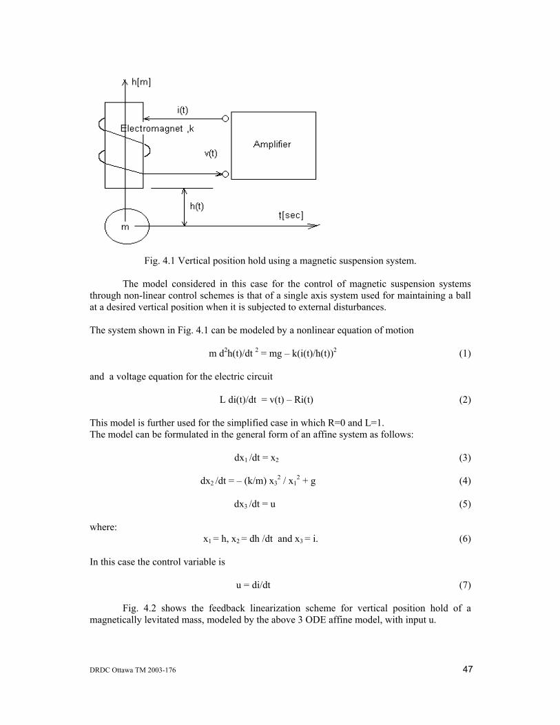
DRDC Ottawa TM 2003-176 47
Fig. 4.1 Vertical position hold using a magnetic suspension system.
The model considered in this case for the control of magnetic suspension systems through non-linear control schemes is that of a single axis system used for maintaining a ball at a desired vertical position when it is subjected to external disturbances. The system shown in Fig. 4.1 can be modeled by a nonlinear equation of motion
m d2h(t)/dt 2 = mg – k(i(t)/h(t))2 (1)
and a voltage equation for the electric circuit
L di(t)/dt = v(t) – Ri(t) (2) This model is further used for the simplified case in which R=0 and L=1. The model can be formulated in the general form of an affine system as follows:
dx1 /dt = x2 (3)
dx2 /dt = – (k/m) x32 / x1
2 + g (4)
dx3 /dt = u (5) where:
x1 = h, x2 = dh /dt and x3 = i. (6) In this case the control variable is
u = di/dt (7) Fig. 4.2 shows the feedback linearization scheme for vertical position hold of a magnetically levitated mass, modeled by the above 3 ODE affine model, with input u.
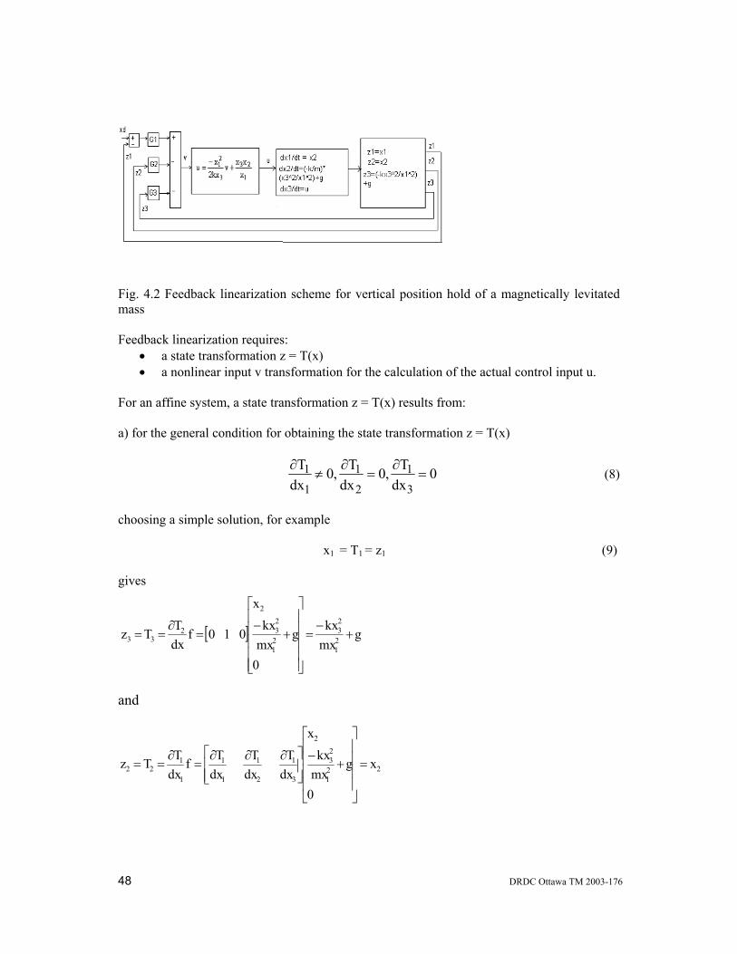
48 DRDC Ottawa TM 2003-176
Fig. 4.2 Feedback linearization scheme for vertical position hold of a magnetically levitated mass Feedback linearization requires:
• a state transformation z = T(x) • a nonlinear input v transformation for the calculation of the actual control input u.
For an affine system, a state transformation z = T(x) results from: a) for the general condition for obtaining the state transformation z = T(x)
0dx
T,0dx
T,0dx
T
3
1
2
1
1
1 =∂
=∂
≠∂
(8)
choosing a simple solution, for example
x1 = T1 = z1 (9) gives
and
[ ] gmxkx
0
gmxkx
x
010fdxT
Tz 21
23
21
23
2
233 +
−=
+−
=∂
==
221
23
2
3
1
2
1
1
1
1
122 x
0
gmxkx
x
dxT
dxT
dxTf
dxTTz =
+−
∂∂∂=
∂==
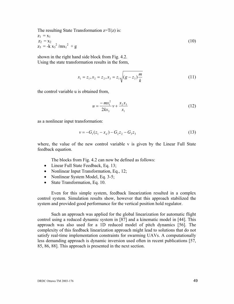
DRDC Ottawa TM 2003-176 49
The resulting State Transformation z=T(z) is: z1 = x1 z2 = x2 (10) z3 = -k x3
2 /mx12 + g
shown in the right hand side block from Fig. 4.2. Using the state transformation results in the form,
kmzgzxzxzx )(,, 3132211 −=== (11)
the control variable u is obtained from,
1
32
3
21
2 xxxv
kxmxu +
−= (12)
as a nonlinear input transformation:
332211 )( zGzGxzGv d −−−−= (13) where, the value of the new control variable v is given by the Linear Full State feedback equation. The blocks from Fig. 4.2 can now be defined as follows:
• Linear Full State Feedback, Eq. 13; • Nonlinear Input Transformation, Eq., 12; • Nonlinear System Model, Eq. 3-5; • State Transformation, Eq. 10.
Even for this simple system, feedback linearization resulted in a complex control system. Simulation results show, however that this approach stabilized the system and provided good performance for the vertical position hold regulator. Such an approach was applied for the global linearization for automatic flight control using a reduced dynamic system in [87] and a kinematic model in [44]. This approach was also used for a 1D reduced model of pitch dynamics [56]. The complexity of this feedback linearization approach might lead to solutions that do not satisfy real-time implementation constraints for swarming UAVs. A computationally less demanding approach is dynamic inversion used often in recent publications [57, 85, 86, 88]. This approach is presented in the next section.
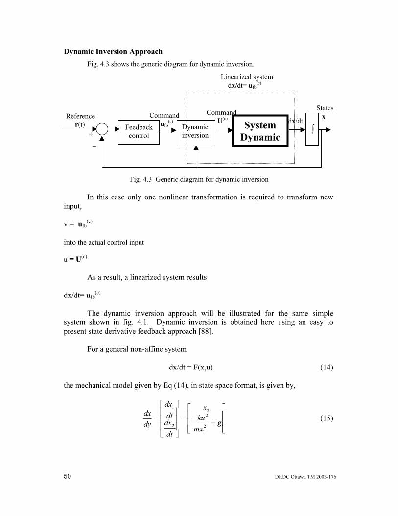
50 DRDC Ottawa TM 2003-176
Dynamic Inversion Approach Fig. 4.3 shows the generic diagram for dynamic inversion.
Fig. 4.3 Generic diagram for dynamic inversion In this case only one nonlinear transformation is required to transform new input, v = ufb
(c) into the actual control input u = U(c) As a result, a linearized system results dx/dt= ufb
(c) The dynamic inversion approach will be illustrated for the same simple system shown in fig. 4.1. Dynamic inversion is obtained here using an easy to present state derivative feedback approach [88]. For a general non-affine system
dx/dt = F(x,u) (14) the mechanical model given by Eq (14), in state space format, is given by,
+−=
= gmxku
x
dtdxdtdx
dydx
21
22
2
1
(15)
dx/dt Feedback control
Reference r(t)
+ _
Command U(c)
Dynamicinversion
Command ufb
(c)
Linearized system dx/dt= ufb
(c)
∫
States x
System Dynamic
DRDC Ottawa TM 2003-176 51
Taking the derivative of Eq. 14
d2x/dt2 = (δF/δx)dx/dt +(δF/δu)du/dt (16) the control variable is obtained in a linear form as du/dt:
or
1
221
2 xuxv
kumx
dtdu
+−= (17)
The nonlinear controllers, given by Eq. 17 and Eq. 12, are restricted to conditions in which the variables u and x1 in Eq. 17 and the variables x1 and x3 in Eq. 12 do not cross zero. This is because of the fact that these variables appear in the denominator of the nonlinear control functions. A PD controller plus acceleration feedback can be chosen for obtaining the new control variable v:
)()(2
2
dpd
dd
a xxKdt
dxdtdxK
dtxdKv −−−−= (18)
For dx2/dt2 =v, the transfer function between xd and x1 is:
pda
p
d KsKsKsK
sxsx
+++= 23
1
)()(
(19)
where the position error, velocity and acceleration feedback gains are Kp, Kd and Ka, respectively. This transfer function (19) shows that the proposed state derivative controller also achieves system linearization. Compared to the feedback linearization controller from the previous section, in this case a third state x3 is not defined, but the resulting du/dt has to be integrated. The fact that no state transformation z = T(x) is required represents an important computation simplification. Simulation results indicate that, again, the response corresponds to a stable system. The steady-state error is very small. The overshoot is high but a better transient performance can be obtained by a more elaborate linear controller design [88]. Dynamic inversion was used for the linearization of the 1D nonlinear model for pitch rate q, as shown in Fig. 4.4. The result is a linearized system,
0duFfor)
dtdx
dxu)F(x,(v
uu)F(x,
dtdu 1
≠∂∂
−
∂∂
=−
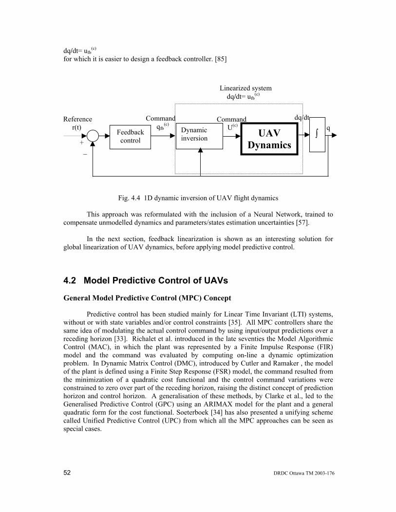
52 DRDC Ottawa TM 2003-176
dq/dt= ufb(c)
for which it is easier to design a feedback controller. [85]
Fig. 4.4 1D dynamic inversion of UAV flight dynamics This approach was reformulated with the inclusion of a Neural Network, trained to compensate unmodelled dynamics and parameters/states estimation uncertainties [57]. In the next section, feedback linearization is shown as an interesting solution for global linearization of UAV dynamics, before applying model predictive control.
4.2 Model Predictive Control of UAVs
General Model Predictive Control (MPC) Concept
Predictive control has been studied mainly for Linear Time Invariant (LTI) systems, without or with state variables and/or control constraints [35]. All MPC controllers share the same idea of modulating the actual control command by using input/output predictions over a receding horizon [33]. Richalet et al. introduced in the late seventies the Model Algorithmic Control (MAC), in which the plant was represented by a Finite Impulse Response (FIR) model and the command was evaluated by computing on-line a dynamic optimization problem. In Dynamic Matrix Control (DMC), introduced by Cutler and Ramaker , the model of the plant is defined using a Finite Step Response (FSR) model, the command resulted from the minimization of a quadratic cost functional and the control command variations were constrained to zero over part of the receding horizon, raising the distinct concept of prediction horizon and control horizon. A generalisation of these methods, by Clarke et al., led to the Generalised Predictive Control (GPC) using an ARIMAX model for the plant and a general quadratic form for the cost functional. Soeterboek [34] has also presented a unifying scheme called Unified Predictive Control (UPC) from which all the MPC approaches can be seen as special cases.
dq/dt
Feedback control
Reference r(t)
+ _
Command U(c) Dynamic
inversion
Command qfb
(c)
Linearized system dq/dt= ufb
(c)
∫ q UAV
Dynamics
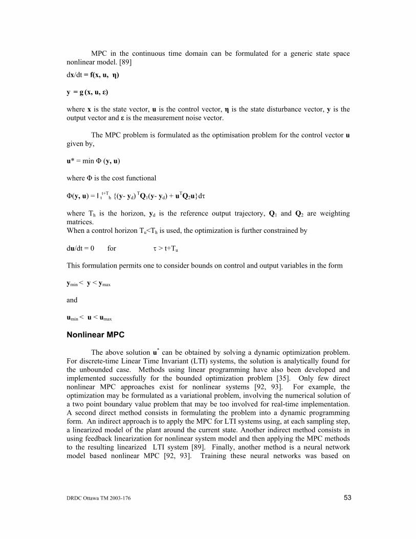
DRDC Ottawa TM 2003-176 53
MPC in the continuous time domain can be formulated for a generic state space nonlinear model. [89]
dx/dt = f(x, u, η) y = g (x, u, ε) where x is the state vector, u is the control vector, η is the state disturbance vector, y is the output vector and ε is the measurement noise vector. The MPC problem is formulated as the optimisation problem for the control vector u given by, u* = min Φ (y, u) where Φ is the cost functional Φ(y, u) = It
t+Th {(y- yd) TQ1(y- yd) + uTQ2u}dτ
where Th is the horizon, yd is the reference output trajectory, Q1 and Q2 are weighting matrices. When a control horizon Tu<Th is used, the optimization is further constrained by du/dt = 0 for τ > t+Tu This formulation permits one to consider bounds on control and output variables in the form ymin < y < ymax and umin < u < umax Nonlinear MPC The above solution u* can be obtained by solving a dynamic optimization problem. For discrete-time Linear Time Invariant (LTI) systems, the solution is analytically found for the unbounded case. Methods using linear programming have also been developed and implemented successfully for the bounded optimization problem [35]. Only few direct nonlinear MPC approaches exist for nonlinear systems [92, 93]. For example, the optimization may be formulated as a variational problem, involving the numerical solution of a two point boundary value problem that may be too involved for real-time implementation. A second direct method consists in formulating the problem into a dynamic programming form. An indirect approach is to apply the MPC for LTI systems using, at each sampling step, a linearized model of the plant around the current state. Another indirect method consists in using feedback linearization for nonlinear system model and then applying the MPC methods to the resulting linearized LTI system [89]. Finally, another method is a neural network model based nonlinear MPC [92, 93]. Training these neural networks was based on
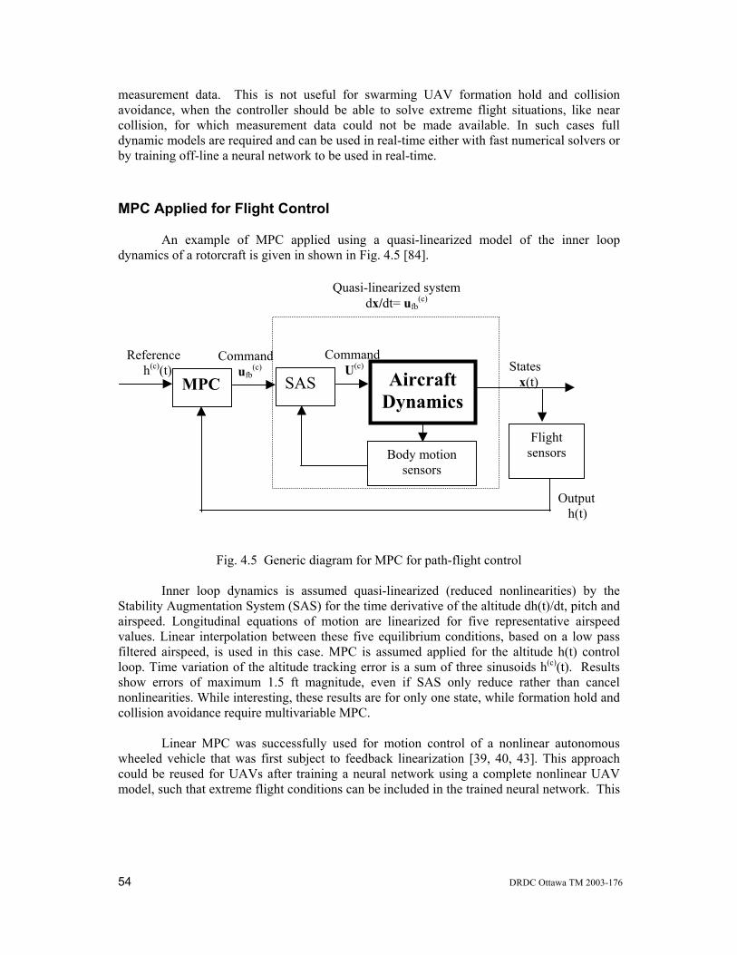
54 DRDC Ottawa TM 2003-176
measurement data. This is not useful for swarming UAV formation hold and collision avoidance, when the controller should be able to solve extreme flight situations, like near collision, for which measurement data could not be made available. In such cases full dynamic models are required and can be used in real-time either with fast numerical solvers or by training off-line a neural network to be used in real-time.
MPC Applied for Flight Control An example of MPC applied using a quasi-linearized model of the inner loop dynamics of a rotorcraft is given in shown in Fig. 4.5 [84].
Fig. 4.5 Generic diagram for MPC for path-flight control Inner loop dynamics is assumed quasi-linearized (reduced nonlinearities) by the Stability Augmentation System (SAS) for the time derivative of the altitude dh(t)/dt, pitch and airspeed. Longitudinal equations of motion are linearized for five representative airspeed values. Linear interpolation between these five equilibrium conditions, based on a low pass filtered airspeed, is used in this case. MPC is assumed applied for the altitude h(t) control loop. Time variation of the altitude tracking error is a sum of three sinusoids h(c)(t). Results show errors of maximum 1.5 ft magnitude, even if SAS only reduce rather than cancel nonlinearities. While interesting, these results are for only one state, while formation hold and collision avoidance require multivariable MPC. Linear MPC was successfully used for motion control of a nonlinear autonomous wheeled vehicle that was first subject to feedback linearization [39, 40, 43]. This approach could be reused for UAVs after training a neural network using a complete nonlinear UAV model, such that extreme flight conditions can be included in the trained neural network. This
Reference h(c)(t)
Command U(c)
Command ufb
(c)
Quasi-linearized system dx/dt= ufb
(c)
States x(t)
Flight sensors
Output h(t)
Body motion sensors
MPC SAS AircraftDynamics
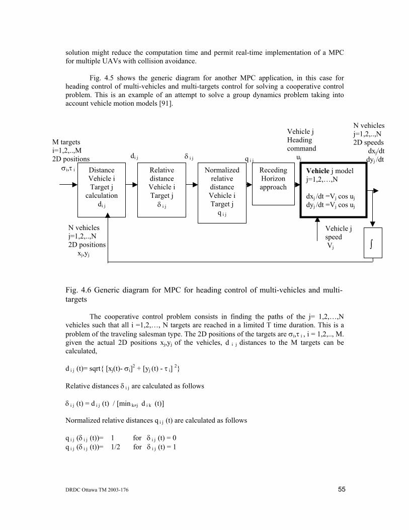
DRDC Ottawa TM 2003-176 55
solution might reduce the computation time and permit real-time implementation of a MPC for multiple UAVs with collision avoidance. Fig. 4.5 shows the generic diagram for another MPC application, in this case for heading control of multi-vehicles and multi-targets control for solving a cooperative control problem. This is an example of an attempt to solve a group dynamics problem taking into account vehicle motion models [91]. Fig. 4.6 Generic diagram for MPC for heading control of multi-vehicles and multi-targets The cooperative control problem consists in finding the paths of the j= 1,2,…,N vehicles such that all i =1,2,…, N targets are reached in a limited T time duration. This is a problem of the traveling salesman type. The 2D positions of the targets are σi,τ i , i = 1,2,.., M. given the actual 2D positions xj,yj of the vehicles, d i j distances to the M targets can be calculated, d i j (t)= sqrt{ [xj(t)- σi]2 + [yj (t) - τ i] 2} Relative distances δ i j are calculated as follows δ i j (t) = d i j (t) / [min k≠j d i k (t)] Normalized relative distances q i j (t) are calculated as follows q i j (δ i j (t))= 1 for δ i j (t) = 0 q i j (δ i j (t))= 1/2 for δ i j (t) = 1
Vehicle j model j=1,2,…,N dxj /dt =Vj cos uj dyj /dt =Vj cos uj
Distance Vehicle i Target j
calculation di j
M targets i=1,2,..,M 2D positions σi,τ i
∫
N vehicles j=1,2,..,N 2D positions xj,yj
Vehicle j speed Vj
Vehicle j Heading command uj
N vehicles j=1,2,..,N 2D speeds dxj/dt dyj /dt δ i j
Relative distance Vehicle i Target j
δ i j
Normalizedrelative distance Vehicle i Target j
q i j
Receding Horizon approach
di j q i j
56 DRDC Ottawa TM 2003-176
lim q i j (δ i j (t))= 0 for δ i j (t) → 4 The receding horizon approach calculates the vehicle j heading command uj using quadratic finite time optimization of, for example, p i j q i j , where p i j (δ i j) is the probability that vehicle j is assigned to target point I when relative distance is δ i j . This formulation is of the MPC type and, in principle, can be solved using dynamic programming. The vehicle model is very simple, a conversion of the velocity from polar Vj (velocity amplitude), uj (heading) components into Cartesian components dxj/dt and dyj/dt. The vehicle velocity amplitude Vj is considered given in this problem, while the heading uj is considered the receding horizon control variable. This approach is an interesting solution to be further developed for swarming UAV flight control. Distributed MPC Distributed MPC is formulated for n-agents (or independent controllers) that can operate independently, but communicate to one another the current values of the control variables. In case that interactions between agents are limited, this approach might be more efficient computationally than the attempt to solve simultaneously the control problem for all agents [91]. The solution to distributed MPC is developed mostly for the case of linear MPC without constraints. This is not surprising given that the nonlinear MPC problem is not yet completely solved for a single agent. Distributed MPC seems, however, particularly suited to solve the problems of swarming UAV control and is definitely worthwhile to be further investigated for this purpose.
4.3 Digital Simulation and Hardware-in-the-loop Simulation of Controllers Digital Simulation Computer simulation of vehicle dynamics is greatly facilitated by the development of graphical programming languages. For example, Simulink and Stateflow were the languages used for a very detailed ground vehicle dynamics simulation using a mechatronics integration of mixed electric, mechanic, combustion and hydraulics subsystems [94]. Similar computer simulation using MATLAB/Simulink was developed for aircraft weapon system models [67]. The simulator includes airframe dynamics, avionics and controller models. MATLAB/Simulink simulators can eventually be made compatible with Real Time Workshop for C code compilation that allows real-time applications. MATLAB/Simulink, Stateflow and Virtual Reality Toolbox were used for simulating multi-UAVs under cooperative control [61]. Fixed targets and obstacles for an arbitrary number of
DRDC Ottawa TM 2003-176 57
UAVs can be simulated and displayed in animation mode. The simulator can be used for testing control algorithms on prototype vehicles. Avionics development requires extensive simulation studies and avionics manufacturers sometimes offer dedicated softwares for aircraft simulator including avionics models. Piccolo system offers this package for its avionics for UAVs [76]. The simulator was presented in Ch. 2. Generic aircraft simulators are Aerospace Blockset from MATHWORKS [78] and AeroSim from Unmanned Dynamics [77]. Aerospace Blockset contains components needed for assembling aircraft digital simulators for testing the autopilot and the navigation system, but lacks aerodynamics blocks. AeroSim has similar characteristics to Aerospace Blockset, but contains aerodynamics blocks. Unified synthetic environment simulators [5, 6] permit operational space simulation and visualization and were presented in Ch. 1.1. Computer simulators permit off-line analysis of prototype vehicles, but are limited by the unmodelled dynamics and parameters/state uncertainty. Actual experimentation overcomes limitations because of unmodelled dynamics and parameters/state uncertainty. Moreover, experiments are avoided for extreme conditions, due to the high cost of vehicle damage, even if the design should be tested for evaluating their performance when such conditions occur. Hardware-In-the Loop (HIL) simulation overcomes such limitations by assembling the vehicle combining computer simulated subsystems with available physical components. Moreover, HIL might be the only solution for evaluating system performance for extreme conditions, as for example near collision conditions or severe atmospheric conditions. The reduction of high mishap rates of UAVs to levels comparable to manned aircraft requires however that such tests are carried out before the whole UAV is available and the tests have to include extreme operating conditions. The high failure rate of UAV avionics cannot be explained and corrected by only testing avionics using the conventional HIL approach, because adjacent subsystems like sensors and actuators contribute to the occurrence of such failures. For this reason, in the next section both conventional and advanced HIL simulators will be presented.
Hardware-in –the Loop Experimentation
Currently, conventional Hardware-in-the-loop simulations are designed for testing physical Electronic Control Units interfaced with digitally simulated vehicles. Advanced hardware-in-the-loop simulators can, however, test active and passive mechanical loads, simulated physically on actual motors, under computer control. Based on the model of the active or passive mechanical load, the motor under digital control is used to emulate the load torque of a passive load not yet available in a physical form [96].
Mechatronic systems, as for example UAVs, are usually very complex systems
consisting of different mechanical, electrical and electronic components. Building such systems could be time demanding and very expensive. Design of each component requires testing. If conducted on real final vehicles, this testing is expensive. Hardware-in-the-loop (HIL) testing can be one solution for such cases.
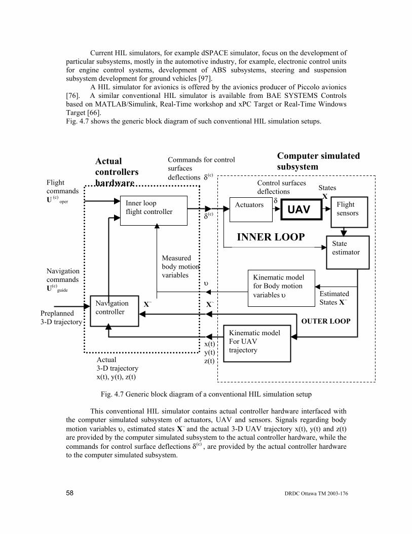
58 DRDC Ottawa TM 2003-176
Current HIL simulators, for example dSPACE simulator, focus on the development of particular subsystems, mostly in the automotive industry, for example, electronic control units for engine control systems, development of ABS subsystems, steering and suspension subsystem development for ground vehicles [97].
A HIL simulator for avionics is offered by the avionics producer of Piccolo avionics [76]. A similar conventional HIL simulator is available from BAE SYSTEMS Controls based on MATLAB/Simulink, Real-Time workshop and xPC Target or Real-Time Windows Target [66]. Fig. 4.7 shows the generic block diagram of such conventional HIL simulation setups.
Fig. 4.7 Generic block diagram of a conventional HIL simulation setup This conventional HIL simulator contains actual controller hardware interfaced with the computer simulated subsystem of actuators, UAV and sensors. Signals regarding body motion variables υ, estimated states X~ and the actual 3-D UAV trajectory x(t), y(t) and z(t) are provided by the computer simulated subsystem to the actual controller hardware, while the commands for control surface deflections δ(c) , are provided by the actual controller hardware to the computer simulated subsystem.
Actual controllers hardware States
X Actuators
Control surfaces deflections δ
Kinematic model for Body motion variables υ
Commands for control surfaces deflections δ(c)
Inner loop flight controller
Measured body motion variables
Flight sensors
State estimator
OUTER LOOP
Navigation controller Preplanned
3-D trajectory
Navigation commands U(c)
guide
Flight commands U (c)
oper
δ(c)
Kinematic model For UAV trajectory
Actual 3-D trajectory x(t), y(t), z(t)
X~
Computer simulated subsystem
X~ Estimated States X~
x(t) y(t) z(t)
υ
INNER LOOP
UAV
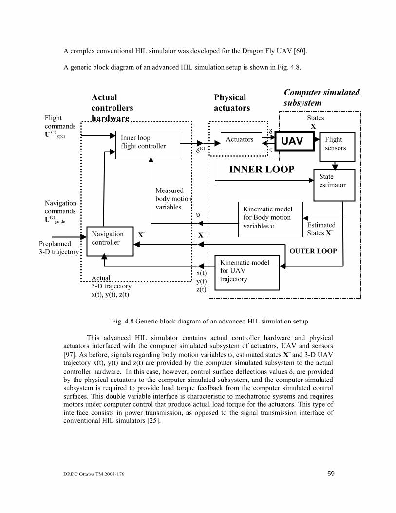
DRDC Ottawa TM 2003-176 59
A complex conventional HIL simulator was developed for the Dragon Fly UAV [60]. A generic block diagram of an advanced HIL simulation setup is shown in Fig. 4.8.
Fig. 4.8 Generic block diagram of an advanced HIL simulation setup This advanced HIL simulator contains actual controller hardware and physical
actuators interfaced with the computer simulated subsystem of actuators, UAV and sensors [97]. As before, signals regarding body motion variables υ, estimated states X~ and 3-D UAV trajectory x(t), y(t) and z(t) are provided by the computer simulated subsystem to the actual controller hardware. In this case, however, control surface deflections values δ, are provided by the physical actuators to the computer simulated subsystem, and the computer simulated subsystem is required to provide load torque feedback from the computer simulated control surfaces. This double variable interface is characteristic to mechatronic systems and requires motors under computer control that produce actual load torque for the actuators. This type of interface consists in power transmission, as opposed to the signal transmission interface of conventional HIL simulators [25].
Actual controllers hardware States
X
Actuators τ
Kinematic model for Body motion variables υ
Inner loop flight controller
Measured body motion variables
Flight sensors
State estimator
OUTER LOOP
Navigation controller Preplanned
3-D trajectory
Navigation commands U(c)
guide
Flight commands U (c)
oper
δ(c)
Kinematic model for UAV trajectory Actual
3-D trajectory x(t), y(t), z(t)
X~
Computer simulated subsystem
X~ Estimated States X~
x(t) y(t) z(t)
υ
Physical actuators
δ UAV
INNER LOOP
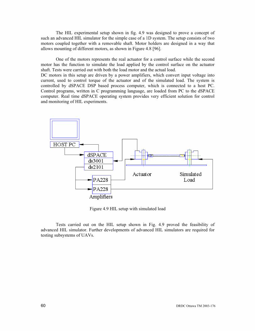
60 DRDC Ottawa TM 2003-176
The HIL experimental setup shown in fig. 4.9 was designed to prove a concept of such an advanced HIL simulator for the simple case of a 1D system. The setup consists of two motors coupled together with a removable shaft. Motor holders are designed in a way that allows mounting of different motors, as shown in Figure 4.8 [96].
One of the motors represents the real actuator for a control surface while the second motor has the function to simulate the load applied by the control surface on the actuator shaft. Tests were carried out with both the load motor and the actual load. DC motors in this setup are driven by a power amplifiers, which convert input voltage into current, used to control torque of the actuator and of the simulated load. The system is controlled by dSPACE DSP based process computer, which is connected to a host PC. Control programs, written in C programming language, are loaded from PC to the dSPACE computer. Real time dSPACE operating system provides very efficient solution for control and monitoring of HIL experiments.
Figure 4.9 HIL setup with simulated load Tests carried out on the HIL setup shown in Fig. 4.9 proved the feasibility of advanced HIL simulator. Further developments of advanced HIL simulators are required for testing subsystems of UAVs.
DRDC Ottawa TM 2003-176 61
5. Conclusions and Recommendations concerning Flight and Mission Control of Swarming UAVs 5.1 Conclusions
1. The current state of Swarming UAV concept development and experimentation can be characterized by a separation between proposed solutions for group dynamics (swarming, tight or large formation flight, leader-followers formation etc), and the proposed solutions for individual UAV flight control. Group dynamics solutions satisfy the needs for strategic and tactical decisions regarding the missions for multi-UAVs, but generally ignore flight dynamic constraints and are not proved applicable, in particular to fixed wing UAVs. Flight control solutions have been tested in realistic simulations and experiments, but do not address the strategic and tactical questions and needs. Intermediate solutions use a simplified flight dynamics model and address only simple group dynamics issues.
2. The specificity of fixed wing UAVs in both individual and group flight cannot be ignored. Marching human formations and a group of bicycle riders cannot realize the same commands, for example, because the bicycle can not achieve lateral motion and is stable only while moving. In general, legged animals and vehicles are omni-directional, while birds, fish, cars and airplanes are not. In this framework, fixed wing UAVs are not omni-directional and cannot fly below certain airspeed. Moreover, control surfaces for aileron, elevator, rudder and thrusters do not permit the application of the lateral forces and achieve closed loop control of lateral motion. These vehicle constraints require the development of group dynamics solutions which take into consideration, from the beginning, that fixed wing UAV motion is only partly controllable.
3. Swarming UAVs can be characterized by the fact that they operate in distinctively
different modes of operation: cruising from initial station to arrive in formation, formation hold, collision avoidance with other UAVs and other moving or fixed obstacles, actual mission, etc. It seems suitable to develop separate and specific controllers for each mode of operation with consideration to possible instability due to switching from one to another controller. Individual UAV flight control can use the extensive experience from autopilot controllers designed for conventional aircrafts, including Stability Augmentation System design. Formation flight should include inter-UAV collision avoidance control using constrained kinematic controllers. Tight formation requires very fast control of inter-UAV clearance using constrained dynamics based controllers, to avoid collision and group instability. Flight controllers for actual missions might replace fuel efficiency criteria by safety and mission success criteria to be developed for specific applications.
62 DRDC Ottawa TM 2003-176
This multitude of controllers has to be experimentally tested to qualify for real-time implementation. Interesting solutions for overall swarming UAV control are Distributed Model Predictive Control and Exact Linearization because of their ability to address both individual UAV flight constraints and group dynamics requirements. A combination of Neural Networks and Fuzzy Controllers, trained to achieve the performance of chosen advanced controllers is an interesting solution to real-time implementation requirements.
4. After the design of swarming UAV controllers, testing cannot be immediately carried
out experimentally because of the fact that when testing collision avoidance, controller failures can result in UAV destruction. For this reason, besides simulation tests, Hardware-In-the-Loop Simulation is required to test actual real-time hardware for controller, actuators, sensors and, possibly, payload. Such a Hardware-In-the-Loop set-up requires interfacing hardware with a dynamic simulation computer using both signal and power (velocity-force/torque) transmission
5.2 Recommendations 1. To satisfy both UAV flight constraints and address actual group dynamics issues,
intensive research on nonlinear dynamics based real time control algorithm is needed with results tested in both virtual environments and by live experimentations.
2. The constraints imposed by the non-holonomicity of fixed wing UAVs require the
development of group dynamics solutions which take into consideration, from the beginning, that fixed wing UAV motion is only partly controllable.
3. Extensive research on Distributed Model Predictive Control and Exact Linearization
is proposed because of their ability to address both individual UAV flight constraints and group dynamics requirements.
4. A combination of Neural Networks and Fuzzy Controllers, trained to achieve the
performance of chosen advanced controllers is an interesting solution to real-time implementation requirements.
5. Hardware-In-the-Loop Simulation is required to test actual real-time hardware for
controller, actuators, sensors and, possibly, payload for the verification of the proposed Swarming UAVs control algorithm and simulation results.
DRDC Ottawa TM 2003-176 63
References [1] ***, Unmanned Aerial Vehicle (UAV) Roadmap, Office of the Secretary of Defense, Department of Defense, 2000, http://www.acq.osd.mil/usd/uav_roadmap.pdf [2] ***, Background Briefing on Unmanned Aerial Vehicles, DoD News Briefing, http://www.fas.org/irp/program/collect/uav_103101.html [3] J. Bovenkamp et al, The Future of Forces Synthetic Environments Section, Land Forces Technical Staff Course, Ottawa, 13 Nov. 2002. [4] ***, SWARMING ENTITIES-the Operational Utilities of Establishing Humans-in- the-Loop, Rapid Assessment Process Report # 02-04, US Joint Forces Command, 3 June 2002. [5] Dickerson, C. and Sabins, M., Coalition Integrated Air Picture Architecture, INCOSE INSIGHT, Oct. 2002, pp. 10-13. [6] ***, Multiple Unified Simulation Environment (MUSE) / Air Force Synthetic Environment for Reconnaissance and Surveillance (AFSERS), JTC/SIL, AMCOM, SED, Redstone Arsenal, Al, Apr. 2002. [7] ***, Vehicle Control Station, presentation at National Defense Headquarters, Ottawa, 18 Oct, 2002, CDL Systems, http://www.cdlsystems.com/ [8] Weiler, D. R. et al, A General Purpose Control Station for Unmanned Vehicles, CDL Systems, 1995, http://www.cdlsystems.com/onlpaper.html [9] Meakin, M. G. and Solomon, J., A General Purpose Control Station for Unmanned Vehicles, AUVSI 2001, CDL Systems, http://www.cdlsystems.com/onlpaper.html [10] ***, RQ-1 Predator MAE UAV, http://www.fas.org/irp/program/collect/predator.htm [11] ***, Shephard’s Unmanned Vehicles Handbook, 2002. [12] ***, Autopilot, http://autopilot.sourceforge.net/ [13] ***, MicroPilot, http://www.uavflight.com/ [14] Lin, C-F, Modern Navigation, Guidance, and Control, vol. II, Prentice Hall, 1991. [15] Fahlstrom, P. G. and Gleason, T. J., Introduction to UAV Systems, UAV SYSTEMS, INC., Second Edition, 1998. [16] Kolk, W. R., Modern Flight Dynamics, Prentice Hall, 1961. [17] McLean, D., Automatic Flight Control Systems, Prentice Hall, 1990. [18] Blakelock, J. H., Automatic Control of Aircraft and Missiles, J. Wiley, 1991. [19] Pachter, M. and Houpis, C. H., Flight Control of Piloted Aircraft, Ch. 75.1 in The Control Handbook, edited by W. Levine, CRC Press, 1996, pp. 1287-1303. [20] Schmidt, L. V., Introduction to Aircraft Flight Dynamics, AIAA, Inc., 1998. [21] Abzug, M., J., Computational Flight Dynamics, AIAA, Inc., 1998. [22] McKinley, J., L. and Bent, R. D., Electricity and Electronics for Aerospace Vehicles, McGraw-Hill, 1971. [23] Shamma, J. S., Linearization and Gain Scheduling, Ch. 20.3 in The Control Handbook, edited by W. Levine, CRC Press, 1996, pp. 388-396. [24] Houpis, C., Quantitative Feedback Theory (QFT) Technique, Ch. 44 in The Control Handbook, edited by W. Levine, CRC Press, 1996, pp. 701-716. [25] Necsulescu, D., Mechatronics, Prentice Hall, 2002.
64 DRDC Ottawa TM 2003-176
[26] Lublin, L. et al, H (LQG) and H Control, Ch. 40 in The Control Handbook, edited by W. Levine, CRC Press, 1996, pp. 651-661. [27] Isidori, A.. and Di Benedetto, M. D, Feedback Linearization of Nonlinear Systems, Ch. 57.1-57.3, in The Control Handbook, edited by W. Levine, CRC Press, 1996, pp. 909-932. [28] Passino, K. M., Intelligent Control, Ch. 57.9, in The Control Handbook, edited by W. Levine, CRC Press, 1996, pp. 994-1001. [29] Passino, K. M. and Yurkovich, S., Fuzzy Control, Ch. 57.10, in The Control Handbook, edited by W. Levine, CRC Press, 1996, pp. 1001-1017. [30] Farrell, J. A., Neural Control, Ch. 57.9, in The Control Handbook, edited by W. Levine, CRC Press, 1996, pp. 1017-1030. [31] Rao, V. and Rao, H., C++ Neural Networks and Fuzzy Logic, MIS Press, 1995. [32] Wen, J., T-U., Control of Nonholonomic Systems, Ch. 76.3, in The Control Handbook, edited by W. Levine, CRC Press, 1996, pp. 1359-1368. [33] Pike, A. W. et al, Predictive Control, Ch. 51, in The Control Handbook, edited by W. Levine, CRC Press, 1996, pp. 805-814. [34] Soeterboek, R., Predictive Control, a Unified Approach, Prentice Hall, 1992. [35] Maciejowski, J.M., Predictive Control with Constraints, Prentice Hall, 2001. [36] Slotine, J. J. and Li, W., Applied Nonlinear Control, Prentice Hall, 1990. [37] B. Friedland, Advanced Control System Design, Prentice Hall, 1996. [38] Baican, R. and Necsulescu, D., Applied Virtual Instrumentation, WIT Press, 2000. [39] D.S. Necsulescu, M. Eghtesad, Task Space Motion Control of Autonomous Planetary Vehicles, CASI Journal, volume 42, No.4, Dec. 1996, pp.200-206. [40] B. Kim, D.Necsulescu, Autonomous Mobile Vehicles for Motion on Uneven and Inclined Surfaces, Electromotion, Quaterly Int. Journal, Vol 5, No. 3, 1998. [41] R. Jassemi-Zargani, D. Necsulescu, Extended Kalman Filter Based Sensor Fusion for Operational Space Control of a Robot Arm, IEEE Trans. On Instrumentation and Measurement, Dec. 2002. [42] D. Necsulescu, J. de Carufel, C.Canudas de Wit, Investigation of the Efficiency of Acceleration Feedback in Servomechanisms with Dry Friction, Dynamics and Control, Vol.7, No. 4, 1997, pp. 377-397. [43] B. Kim, D.S. Necsulescu, S. Kalaycioglu, Dynamics Control of an Autonomous Wheeled
Ground Vehicle, Transactions CSME, Vol.17, No.4B, 1993, pp. 735-758. [44] I.-J. Ha and S. Chong, Design of a CLOS Guidance Law Via Feedback Linearization,
IEEE Trans. on Aerospace Electronic Systems, Vol. 28, No. 1, Jan. 1992, pp. 51-63. [45] B., Bhanu et al., A System for Obstacle Detection During Rotocraft Low Altitude Flight,
IEEE Trans. on Aerospace Electronic Systems, Vol. 32, No. 3, July 1996, pp. 875-896. [46] D. Boyle and G. Chamidoff, Autonomous Maneuver Tracking for Self-Piloted Vehicles,
Journal of Guidance, Control and Dynamics, vol. 22, No. 1, Jan.-Febr. 1999, pp. 58-67. [47] M.S. de Queiroz et al., Adaptive Nonlinear Control of Multiple Spacecraft Formation
Flying, Journal of Guidance, Control and Dynamics, vol. 23, No. 3, May-June 2000, pp. 385-390.
[48] V. Kapila et al. Spacecraft Formation Flying: Dynamics and Control, Journal of Guidance, Control and Dynamics, vol. 23, No. 3, May-June 2000, pp. 561-564.
[49] J.L. Crassidis and S.R. Vadali, Optimal Variable-Structure Control Tracking of Spacecraft Maneuvers, Journal of Guidance, Control and Dynamics, vol. 23, No. 3, May-June 2000, pp. 564-567.
DRDC Ottawa TM 2003-176 65
[50] M. Pachter et al., Tight Formation Flight Control, Journal of Guidance, Control and Dynamics, vol. 2Journal of Guidance, Control and Dynamics, vol. 24, No. 2, March-Apr 2001, pp. 246-254.
[51] J. Z. Sasiadek and I. Duleba, 3D Local Trajectory Planner for UAV, Journal of Intelligent and Robotic Systems, Vol. 29, 2000, pp. 191-210.
[52] E. Rimon and D.E. Koditschek, Exact Robot Navigation Using Artificial Potential Functions, IEEE Trans. on Robotics and Automation, Vol. 8, No. 5, Oct. 1992, pp. 501-518.
[53] B.A. Kumar and D. Ghose, Radar-Assisted Collision Avoidance/Guidance Strategy for Planar Flight, IEEE Trans. on Aerospace Electronic Systems, Vol. 37, No. 1, Jan 2001, pp. 77-90.
[54] R.M. Botez et al, Optimal Control Laws for Gust Alleviation, Canadian Aeronautics and Space Journal, Vol. 47, No. 1, March 2001.
[55] C-M. Lin and Y.J. Mon, Fuzzy-Logic-Based CLOS Guidance Law Design, , IEEE Trans. on Aerospace Electronic Systems, Vol. 37, No. 2, Apr. 2001, pp. 719-727.
[56] S-Y. Lee et al., Nonlinear Autopilot for High Maneuverability of Bank-to-Turn Missiles, , IEEE Trans. on Aerospace Electronic Systems, Vol. 37, No. 4, July 2001, pp. 1236-1252.
[57] C. J. Schumacher and R. Kumar, Adaptive Control of UAVs in Closed-Coupled Formation Flight, Proc. ASC-1999-2590 .
[58] C. J. Schumacher and S.N. Singh, Nonlinear Control of Multiple UAVs in Close-Coupled Formation Flight, AIAA Conf., AIAA 200-4373.
[59] K. Grossman et al., An Architecture for Multi-Vehicle Autonomy with Small UAVs, www.jhuapl.edu
[60] J. S. Jang and C. J. Tomlin, Autopilot Design for the Stanford DragonFly UAV: Validation through Hardware-in-the-Loop Simulation, AIAA GNC Conf. 2001, Paper AIAA 2001-4179.
[61] D. Lluch, Building Multi-UAV Simulation Methods, AIAA Paper 2002-4977. [62] Y. Yang et al., Decentralized Cooperative Search in UAV’s Using Opportunistic
Learning, AIAA GNC Conf. 2002, Paper AIAA 2002-4590. [63] W. M. McEneaney and B. Fitzpatrick, Control of UAV Operations under Imperfect
Information, Proc. AIAA Technical Conf. and Workshop on Unmanned Aerospace Vehicles, Systems and Technology, 2002, AIAA Paper 2002-3418.
[64] M. flint et al., Cooperative Path-planning for Autonomous Vehicles using Dynamic Programming, 15th Trienal World Congress, 2002 IFAC.
[65] M. Flint et al., Cooperative Control for Multiple Autonomous UAV’s Searching for Targets, CDC 2002.
[66] F. Liang, Rapid Development of UAV Autopilot using MATLAB/ Simulink, Paper AIAA 2002-4976.
[67] T. R. Persing and D. A. Hardaker, Development of Integrated Aircraft Weapon System Models in MATLAB/Simulink, Paper AIAA 2002-5041.
[68] E. P. Anderson and R. W. Beard, An Algorithmic Implementation of Constrained Extremal Control for UAVs, AIAA GNC Conf. 2002, Paper AIAA 2002-4470.
[69] P. Drewes, Lessons Learned in Group Robotic Command and Control, Science Application International Corporation.
[70] S. Brueckner and H. Van Dyke Parunak, Multiple Pheronems for Improved Guidance, Proc. Of Symposium on Advanced Enterprise Control, 2000.
66 DRDC Ottawa TM 2003-176
[71] H. Van Dyke Parunak et al., Digital Pheronems for Autonomous Coordination of Swarming UAVs, AIAA 1st Technical Conf. and Workshop on Unmanned Aerospace Vehicles, Systems and Technology, 2001.
[72] E. Bonabeau, M, Dorigo and G. Theraulaz, Swarm Intelligence: From Natural to Artificial Systems Swarm Intelligence, Oxford University Press, 1999. [73] H. Van Dyke Parunak et al., Mechanisms and Military Applications for Synthetic
Pheronems, Proc. Workshop on autonomy Oriented Computation, Agents 2001, 2001, pp. 58-67.
[74] H. Van Dyke Parunak et al., Distinguishing Environmental and Agent dynamics: a Case Study in Abstraction and Alternate Modeling Technologies, 2001. [75] B. Stevens and F. Lewis, Aircraft Control and Simulation, J. Wiley, 1992. [76] Piccolo System User Guide, http://www.cloudcaptech.com/piccolo.htm [77] User’s Guide. AeroSim, aeronautical simulation blockset, version 1.01, www.u- dynamics.com [78] Aerospace Blockset, MathWorks, www.mathworks.com [79] F. Cellier, Artificial Neural Networks and Genetic Algorithms, Ch. 14 in Continuous Systems Modelling, Springer Verlag, 1991. [80] A. Draeger et al, Model Predictive Control Using Neural Networks, IEEE Control Systems, Oct. 1995, pp. 61-66. [81] F-S. Ho and P. Ioannou, Traffic Flow Modeling and Control Using Artificial Neural Networks, IEEE Control Systems, Oct. 1996, pp. 16-26. [82] J. Kuschewski et al., Application of Feedforward Neural Networks to Dynamical System Identification and Control, IEEE Trans. on Control Systems Technology, vol. 1, No. 1, March 1993, pp. 37-49. [83] Kwong, W.A. et al., Expert supervision of fuzzy learning systems for fault tolerant aircraft control, Proc. IEEE, Vol. 83, No. 3, 1995. [84] D. Swaroop, and J. K. Hedrick, Constant Spacing Strategies for Platooning in Automated Highway Systems, Trans. of the ASME, vol. 121, Sept. 1999, pp. 462-470. [85] J. Reiner et al, Robust dynamic Inversion for Control of Highly Maneuverable Aircraft, J.
of Guidance, Control and Dynamics, Vol. 18, No. 1, Jan-Febr 1995, pp 18-24. [86] S. Lane and R. Stengel, Flight Control Design using Non-Linear Inverse Dynamics,
Automatica, Vol. 24, No. 4, 1988, pp. 471-483. [87] G. Meyer et al, Application of Nonlinear Transformations to Automatic Flight Control,
Automatica, Vol. 20, No. 1, 1984, pp. 103-107. [88] D. Necsulescu, M. Ceru, Nonlinear Control of Magnetic Bearings, Journal of Electrical Engineering, vol. 2, 2002. [89] J. de Carufel, D. Necsulescu, model Predictive Control for Impact/Contact Motion of a Manipulator, Proc. 1995 Can. Conf. on electrical and Compute Engineering, 1995, pp. 330-333. [90] D. Necsulescu, G. Basic, Analysis and Implementation Issues for Haptic Interfaces using HIL Concept, Proc. IEEE Int. Workshop on Haptic Virtual Environments and their Applications, Nov. 2002. [91] E. Camponogara et al., Distributed Model Predictive Control, IEEE Control Systems Magazine, Febr. 2002, pp. 44-51. [92] A. Draeger et al, Model Predictive Control using Neural Networks, IEEE Control Systems, Oct. 1995, pp. 61-66. [93] S. Piche et al, Nonlinear Model Predictive Control Using Neural Networks, IEEE Control Systems Magazine, June 2000, pp. 53-62.
DRDC Ottawa TM 2003-176 67
[94] Using Simulink and Stateflow in Automotive Applications, Marhworks, ftp.Mathworks.com/pub/product-info/examples/autobook.zip [95] C. Cassandras, and W. Li, A receding Horizon approach for Solving Some Cooperative Control Problems, Proc. 41-th IEEE Conf on Decision and Control, Dec. 2002, pp. 3760-3765. [96] D. Necsulescu and G. Basic, Analysis of Implementation Issues using HIL Concept, IEEE Int. Workshop on virtual Environments and Their Applications, Nov. 2002. [97] dSPACE Vehicle Dynamics Simulator, dSPACE, 2000.
68 DRDC Ottawa TM 2003-176
List of symbols/abbreviations/acronyms/initialisms
ARIMAX Auto-Regressive Integrated Moving Average with eXternal Input
DMC Dynamic Matrix Control
DND Department of National Defence
DSP Digital Signal Processor
FIR Finite Impulse Response
FSR Finite Step Response
GCS Ground Control Station
GPC Generalized Predictive Control
GPS Global Positioning System
HIL Hardware In the Loop
INS Inertial Navigation System
LOS Line of Sight
LQ Linear Quadratic
LQG Linear Quadratic Gaussian
LTI Linear Time Invariant
MAC Model Algorithmic Control
MIMO Multi-Input, Multi-Output
MPC Model Predictive Control
MUSE Multiple Unified Simulation Environment
NN Neural Networks
ODE Ordinary Differential Equation
DRDC Ottawa TM 2003-176 69
PD Proportional, Derivative
PID Proportional, Integral, and Derivative
PWM Pulse Width Modulation
RACAGS Radar Assisted Collision Avoidance/Guidance Strategy
RPV Remotely Piloted Vehicle
SAS Stability Augmentation System
UAV Unmanned Aerial Vehicle
UPC Unified Predictive Control
VTOL Vertical Take Off and Landing

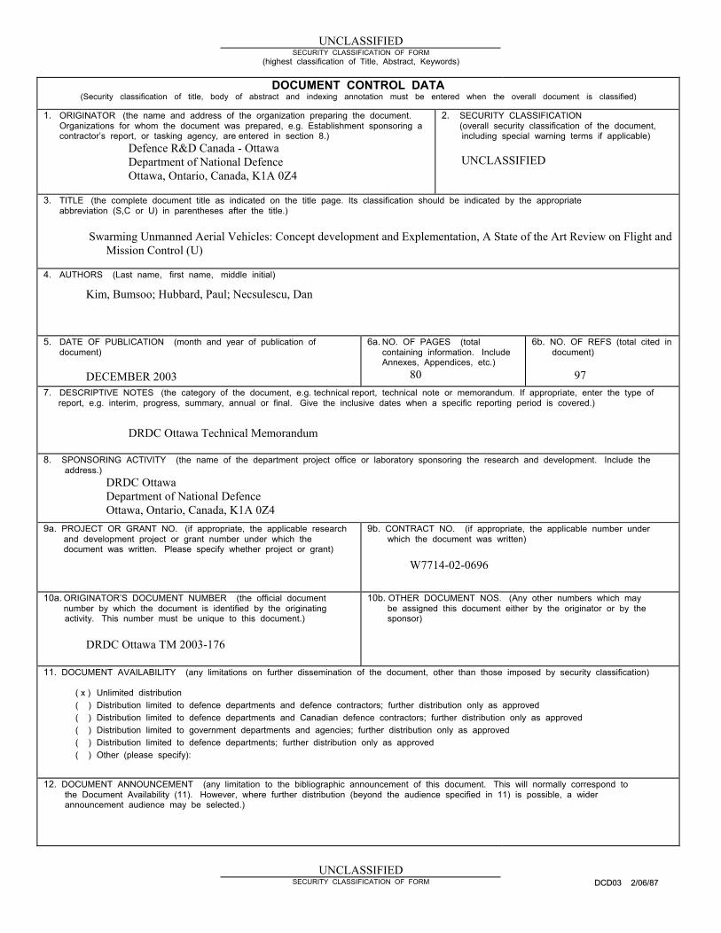
UNCLASSIFIED SECURITY CLASSIFICATION OF FORM
(highest classification of Title, Abstract, Keywords)
DOCUMENT CONTROL DATA (Security classification of title, body of abstract and indexing annotation must be entered when the overall document is classified)
1. ORIGINATOR (the name and address of the organization preparing the document. Organizations for whom the document was prepared, e.g. Establishment sponsoring a contractor’s report, or tasking agency, are entered in section 8.)
Defence R&D Canada - Ottawa Department of National Defence Ottawa, Ontario, Canada, K1A 0Z4
2. SECURITY CLASSIFICATION (overall security classification of the document,
including special warning terms if applicable) UNCLASSIFIED
3. TITLE (the complete document title as indicated on the title page. Its classification should be indicated by the appropriate abbreviation (S,C or U) in parentheses after the title.)
Swarming Unmanned Aerial Vehicles: Concept development and Explementation, A State of the Art Review on Flight and
Mission Control (U)
4. AUTHORS (Last name, first name, middle initial)
Kim, Bumsoo; Hubbard, Paul; Necsulescu, Dan
5. DATE OF PUBLICATION (month and year of publication of document)
DECEMBER 2003
6a. NO. OF PAGES (total containing information. Include Annexes, Appendices, etc.)
80
6b. NO. OF REFS (total cited in document)
97
7. DESCRIPTIVE NOTES (the category of the document, e.g. technical report, technical note or memorandum. If appropriate, enter the type of report, e.g. interim, progress, summary, annual or final. Give the inclusive dates when a specific reporting period is covered.)
DRDC Ottawa Technical Memorandum
8. SPONSORING ACTIVITY (the name of the department project office or laboratory sponsoring the research and development. Include the address.)
DRDC Ottawa Department of National Defence Ottawa, Ontario, Canada, K1A 0Z4
9a. PROJECT OR GRANT NO. (if appropriate, the applicable research and development project or grant number under which the document was written. Please specify whether project or grant)
9b. CONTRACT NO. (if appropriate, the applicable number under which the document was written)
W7714-02-0696
10a. ORIGINATOR’S DOCUMENT NUMBER (the official document number by which the document is identified by the originating activity. This number must be unique to this document.)
DRDC Ottawa TM 2003-176
10b. OTHER DOCUMENT NOS. (Any other numbers which may be assigned this document either by the originator or by the sponsor)
11. DOCUMENT AVAILABILITY (any limitations on further dissemination of the document, other than those imposed by security classification) ( x ) Unlimited distribution ( ) Distribution limited to defence departments and defence contractors; further distribution only as approved ( ) Distribution limited to defence departments and Canadian defence contractors; further distribution only as approved ( ) Distribution limited to government departments and agencies; further distribution only as approved ( ) Distribution limited to defence departments; further distribution only as approved ( ) Other (please specify):
12. DOCUMENT ANNOUNCEMENT (any limitation to the bibliographic announcement of this document. This will normally correspond to
the Document Availability (11). However, where further distribution (beyond the audience specified in 11) is possible, a wider announcement audience may be selected.)
UNCLASSIFIED
SECURITY CLASSIFICATION OF FORM DDCCDD0033 22//0066//8877
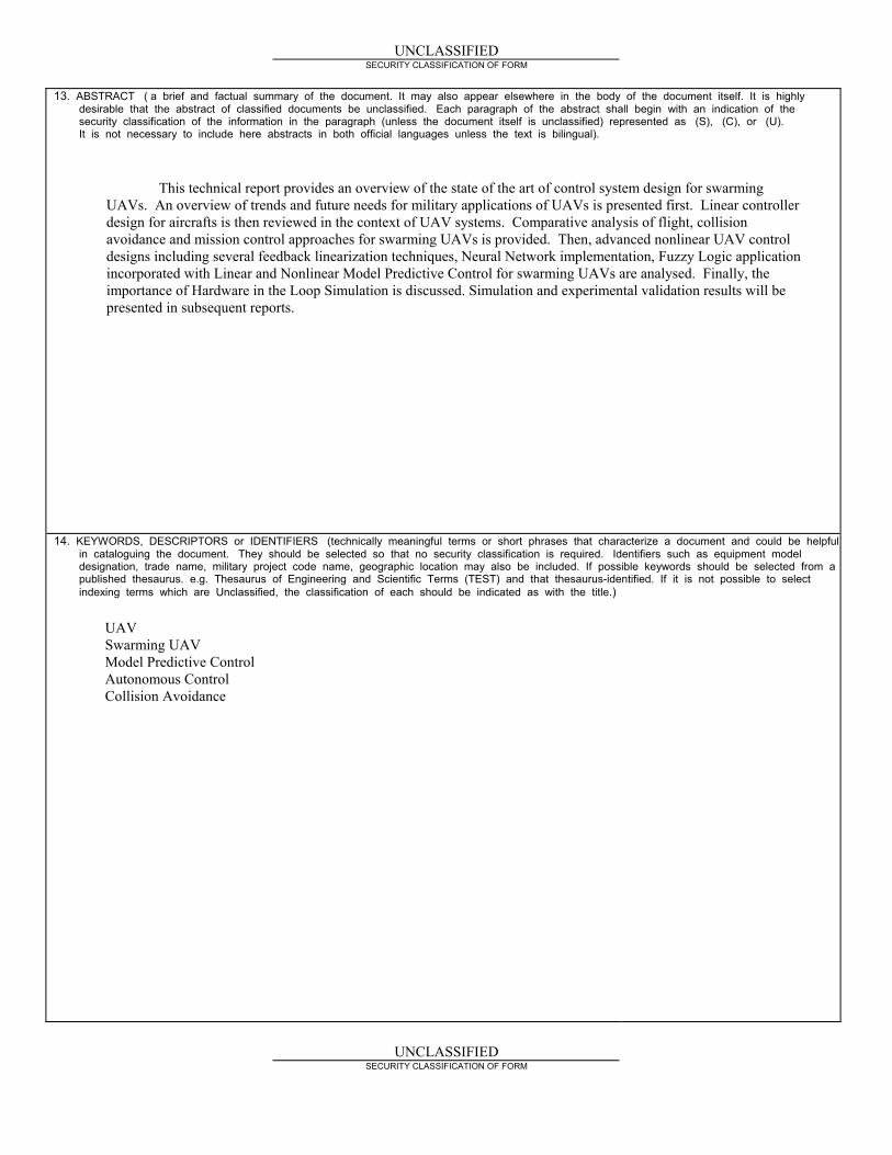
UNCLASSIFIED SECURITY CLASSIFICATION OF FORM
13. ABSTRACT ( a brief and factual summary of the document. It may also appear elsewhere in the body of the document itself. It is highly desirable that the abstract of classified documents be unclassified. Each paragraph of the abstract shall begin with an indication of the security classification of the information in the paragraph (unless the document itself is unclassified) represented as (S), (C), or (U). It is not necessary to include here abstracts in both official languages unless the text is bilingual).
This technical report provides an overview of the state of the art of control system design for swarming UAVs. An overview of trends and future needs for military applications of UAVs is presented first. Linear controller design for aircrafts is then reviewed in the context of UAV systems. Comparative analysis of flight, collision avoidance and mission control approaches for swarming UAVs is provided. Then, advanced nonlinear UAV control designs including several feedback linearization techniques, Neural Network implementation, Fuzzy Logic application incorporated with Linear and Nonlinear Model Predictive Control for swarming UAVs are analysed. Finally, the importance of Hardware in the Loop Simulation is discussed. Simulation and experimental validation results will be presented in subsequent reports.
14. KEYWORDS, DESCRIPTORS or IDENTIFIERS (technically meaningful terms or short phrases that characterize a document and could be helpful in cataloguing the document. They should be selected so that no security classification is required. Identifiers such as equipment model designation, trade name, military project code name, geographic location may also be included. If possible keywords should be selected from a published thesaurus. e.g. Thesaurus of Engineering and Scientific Terms (TEST) and that thesaurus-identified. If it is not possible to select indexing terms which are Unclassified, the classification of each should be indicated as with the title.)
UAV Swarming UAV Model Predictive Control Autonomous Control Collision Avoidance
UNCLASSIFIED
SECURITY CLASSIFICATION OF FORM

Defence R&D Canada
Canada’s leader in defenceand national security R&D
Chef de file au Canada en R & Dpour la défense et la sécurité nationale
R & D pour la défense Canada
www.drdc-rddc.gc.ca