IFN Working Paper No. 977, 2013 Swedish Labor Income Taxation (1862–2013) Gunnar Du Rietz, Dan Johansson and Mikael Stenkula

Research Institute of Industrial Economics P.O. Box 55665

SE-102 15 Stockholm, Sweden info@ifn.se www.ifn.se

Swedish Labor Income Taxation (1862–2013)*

Gunnar Du Rietza Dan Johanssonb, c Mikael Stenkulaa

September, 2015

Abstract: This paper presents annual Swedish time-series data on the top marginal tax wedge and marginal tax wedges on labor income for a low-, average- and high-income earners for the period 1862 to 2013. The tax wedges were initially low and the tax system proportional. The tax wedges began to increase during World War I. The increase accelerated during World War II and through the post-war period. In the 1970s, the top marginal tax wedge was occasionally as high as 90 percent. The main explanations for this development were temporary crises that led to permanent tax increases, the expansion of the public sector and distributional ambitions, bracket creep and the introduction of employer-paid social security contributions. The 1990–1991 tax reform represents the beginning of a new and continuing period of decreasing marginal tax wedges.

JEL-codes: H21, H31, N44 Keywords: Labor income taxation, Marginal tax rate, Marginal tax wedge, Tax reforms.

a Research Institute of Industrial Economics (IFN)

bÖrebro University School of Business

c HUI Research

P.O. Box 55665 SE – 102 15 Stockholm Sweden

SE – 701 82 Örebro Sweden

SE – 103 29 Stockholm Sweden

* This is the working paper version of a chapter with the same title published in Swedish Taxation: Developments since 1862 (ch. 2, pp. 35–122), edited by Magnus Henrekson and Mikael Stenkula, New York: Palgrave Macmillan. Du Rietz and Stenkula gratefully acknowledge financial support from the Jan Wallander and Tom Hedelius Research Foundation and from Finanspolitiska Forskningsstiftelsen. Johansson gratefully acknowledges financial support from the Ragnar Söderberg Foundation. We are grateful for comments on an earlier version from Krister Andersson, Niclas Berggren, Henrik Lindberg, Sven-Olof Lodin, Enrique Rodriguez, Hans Sjögren, Anders Gustafsson and Hans Westerberg (Anders Gustafsson and Hans Westerberg also collected data for several of the tables in the appendices), and seminar participants at the Institute for Economic and Business History Research (EHFF), the Stockholm School of Economics, the 12th Annual SNEE European Integration Conference in Mölle and the 77th Annual Meeting of the Southern Economic Association.

1. Introduction

The tax system is one of society’s most fundamental institutions, as taxation has profound

effects on many economic decisions, such as labor supply, savings and investments. Taxation

of the factors of productionparticularly labor and capital incomehas attracted particular

interest, because taxation is a major determinant of their quantity, quality and usage over time.

This paper studies income taxes on labor. The purpose is to analyze how the taxation of labor

income has developed over time.

Much research on labor taxation addresses the effects of marginal taxation

because it influences (among other things) labor supply in hours, effort at work, efficiency at

work, educational investment, and the timing of consumption.1 Therefore, we would also

expect changes in marginal tax rates to influence the growth rates of taxable income, real

gross domestic product (GDP) and other macroeconomic aggregates.

Although the effects of the tax system have been studied extensively, the results

of these studies are often complex and ambiguous. Empirically, problems repeatedly arise

because the effects of taxation should be assessed over long time spans; however, data are

generally available only for relatively short periods. Hence, there is a need for long

homogenous time series on taxation, which can further our understanding of the tax system’s

structure and its role in industrialization, wealth and structural change.

Rather than examining the effect from one narrow form of taxation (e.g., the

marginal income tax on labor), a wider measuresuch as the marginal tax wedge on labor

incomeis often preferable.2 The marginal tax wedge on labor income incorporates marginal

income taxes, marginal social security contributions and marginal payroll taxes. In addition,

consumption taxes are sometimes included, and social security contributions can also be

adjusted to include only the fiscal component. This measure better captures how individual

1A distinction is frequently made between intensive and extensive marginal decisions. The intensive marginal decision that affects the number of work hours and effort expended by those already employed is mainly influenced by the marginal tax rates. The extensive marginal decision that affects the incentive to participate in the labor market is mainly influenced by the average tax rates. 2 This wider measure is preferable because several forms of taxation affect individual choices. The marginal income tax rate captures the effect from one form, i.e., the income tax on labor, whereas the marginal tax wedge incorporates the effects from other taxes as well. For instance, the incentive effect of employer-paid social security contributions can be substantial, and it has thus been argued that a tax measure that considers the combined effects from different taxes better captures the behavioral effects of taxation. See, e.g., Agell, Englund and Södersten (1998) or Sørensen (2004) for a thorough discussion.

decision making is affected and is also the main determinant of the excess burden resulting

from taxation, that is, distortionary costs in the economy.3

We calculate the long-term evolution of marginal tax wedges on labor income

for Sweden. To finance the rise of the welfare state, the Swedish tax-to-GDP ratio increased

from one of the lowest among Western countries at the beginning of the twentieth century to

the highest in the world by the mid-1960s (Rodriguez 1981). The Swedish tax-to-GDP ratio

remained the highest in the world until 2002, when it was surpassed by Denmark.4

Considered as the “archetype” of the welfare state, Sweden has attracted the attention of

researchers and policymakers and sparked an unsettled debate focused on the possibility of

combining high taxes and economic growth (Esping-Andersen 1990; Henrekson 1996;

Lindbeck 1997; Madrick 2009; Bergh 2014). As a neutral country during both World Wars,

Sweden avoided massive destruction, making long-run analysis appropriate, as these events

profoundly affected the long-term outcome patterns of many other European countries.

Sweden also has excellent tax records, which greatly facilitates our analysis.

As marginal tax wedges often change with income, it is not possible to derive

one measure of the marginal tax wedge that is valid for all incomes. We therefore compute the

top marginal tax wedge and the marginal tax wedge for a high-, average- and low-income

earner.

Our analysis begins in 1862 when Sweden implemented a major new state

(central government) tax system. The decades around the 1850s are historically important, as

the Swedish economy was extensively deregulated, industrialization began and economic

growth took off.5 Hence, we will exploit official statistics and tax laws to describe more than

150 years of tax rates.

Marginal tax rates on labor income, particularly top marginal tax rates, for

several countries (including Sweden) have been the subject of a number of studies.6 For

3 Furthermore, the excess burden is not a linear function of the marginal tax wedge but an increasing convex function, i.e., the burden increases disproportionately faster than the marginal tax wedge, which implies large distortion costs at high tax levels, see Hansson (2000) or Jaimovich and Rebelo (2012). 4 See, e.g., http://stats.oecd.org/Index.aspx?DataSetCode=REV. 5 The tax system is less well documented during the nineteenth century. For example, tax tables reporting income brackets and tax rates have not been compiled and are not readily available. Part of our study has been devoted to going through all the issues of SFS in Riksdagsbiblioteket (the Riksdag Library) to include all tax tables for the earlier period of our examination. SFS (svensk författningssamling) is the Swedish code of statutes and official publication of laws enacted by the Swedish Parliament (Riksdag). 6 See, e.g., Roine, Vlachos and Waldenström (2009) and Rydqvist, Spizman and Strebulaev (2014). Historical studies of the Swedish tax system include Eberstein (1929, 1937), Genberg (1942), Elvander (1972), Hedlund-Nyström (1972), Jakobsson and Normann (1974), Rodriguez (1980), Rodriguez (1981), Gårestad (1987), Dahlgren and Stadin (1990), Du Rietz (1994), Söderberg (1996) and Löwnertz (2003). These studies incorporate extensive information about the Swedish tax system, and some of the results in our paper are derived from these

example, country-specific analyses covering marginal tax rates have been performed for the

U.S. (Barro and Sahasakul 1986; Poterba 2004; Saez 2004), the U.K. (Orhnial and Foldes

1975) and Germany (Corneo 2005). However, none of these studies extends as far back as

1862, and these studies have not calculated the marginal tax wedge on labor income. Neither

has the income at which the top marginal tax wedge begins to be applied been calculated.

Hence, no one has thus far generated this type of data for Sweden, and we are unaware of any

international study covering an equally long time span. Together with tax data for other

economies, our data can be used to conduct long-term comparative analyses among countries.

This paper is organized as follows. In the next section, the marginal tax wedge

on labor income is defined. Section 3 describes the different parts of the marginal tax wedge.

Section 4 presents the evolution of marginal tax wedges on labor income. Section 5

concludes. Appendix A presents the sources underlying the calculations. Alternative

computations concerning marital and household status are presented in Appendix B. In

Appendix C, our results concerning tax rates and tax wedges are reported. Appendices D to J

present extensive data, including all tax tables for the period examined, which enables the

reader to calculate the marginal tax wedges for any income over the entire 1862–2013

period.7

2. The marginal tax wedge on labor income

2.1 Definition

Taxes on labor income drive a wedge between the price of labor paid by firms, and the net

return on labor received by employees. This difference is formally called the tax wedge on

labor income (or tax wedge for short). The tax wedge may influence the incentive to supply

and demand labor, the magnitude of taxable income and the wage formation process. To

further cross-country and longitudinal comparisons, we follow the standard of OECD (2011)

and calculate the marginal tax wedge, tw, as follows:

sources. Only Du Rietz has previously compiled longer time series of the marginal tax wedge. The most recent update, which covers the period 1952–2003, is published in Johansson (2004, 93–94, Table A1). 7 Appendix C reports annual data on wages, marginal tax rates and marginal tax wedges for the three investigated income categories. It also shows the top marginal tax rates, the top marginal tax wedge, the wage when the top marginal tax wedge begins to be applied and the relative top tax income threshold defined as the wage at which the top marginal tax wedge begins to be applied divided by the average annual wage of a production worker. Appendix D reports annual data on local income tax rates, consumption tax rates, state income tax rates and extra taxes, such as the defense tax. Appendix E reports the basic local and state income tax allowances. Appendices F, G and H report employee-paid social security contributions. Appendix I reports the earned income tax credit, and Appendix J reports employer-paid social security contributions.

(1)

where t1 is the marginal income tax; t2 is the marginal social security contributions (SSCs)

paid by employees; and t3 is the marginal SSCs, including payroll taxes, that are added to the

wage and paid by employers. The marginal tax wedge measures the difference between the

total labor costs paid by employers and the net wage received by employees as a result of a

marginal increase in labor income. The wedge is expressed as a percentage of the change in

labor compensation, including SSCs.

Alternative definitions of the tax wedge add consumption taxes or adjust for the

estimated benefit component of SSCs. The reason for the OECD to exclude consumption

taxes is mainly methodological; data are occasionally missing or not sufficiently detailed, and

there is no agreed-upon method to make the estimations comparable across countries when

including them.8 However, for a long-term single country study of Sweden, it is possible to

include consumption taxes in a consistent manner for a comparison over time. Hence, in the

main text, we have calculated the tax wedge by excluding (Section 4.1) and including

(Section 4.4) consumption taxes. Including consumption taxes, the definition of the marginal

tax wedge is:

(2)

where t1 is the marginal income tax, t2 is the marginal SSCs paid by employees, t3 is the

marginal SSCs that are added to the wage and paid by employers and t4 is the marginal

consumption tax rate.

The inclusion or exclusion of consumption taxes will not alter our general

conclusions. Likewise, the long-term evolution of the tax wedges remains the same if we also

adjust the SSC for the estimated benefit component; see Appendix B.

2.2 Taxpayer characteristics

In 1972, the OECD began to report wage data on the average production worker, which was

defined as the average gross wage earnings of adult, full-time manual workers in industry

8 See OECD (2009) for a further discussion of consumption taxes. The treatment of consumption taxes is also theoretically disputed (de Haan, Sturm and Volkerink 2004). Some proponents, such as Heady (2004), argue that consumption and income taxes will broadly have the same effect on the labor market and that it is the sum of these taxes that matters (a uniform sales tax will have the same effect as a proportional income tax on a worker who does not save). However, others argue that consumption taxes should not be included in the wedge because these taxes affect workers and non-workers alike (see the discussion in Daveri and Tabellini 2000, Immervoll 2004, Heady 2004 and Bassanini and Romain 2006).

)1()1)(1(

13

21

ttt

tw +−−

−=

)1()1)(1)(1(

13

421

tttt

t w +−−−

−=

sector D in the International Standard Industrial Classification of all Economic Activities,

Revision 3 (ISIC Rev. 3). In 1979, the series on wage data were complemented with

calculations on average tax rates and average tax wedges for two family types (single person

and one-earner married couple) that were earning 100 percent of the average annual wage of a

production worker (henceforth denoted APW). In 1997, the analysis was expanded to

incorporate 12 tax measures (including marginal tax measures) for eight different types of

taxpayers, characterized by different family status (single/married, 0–2 children), economic

status (one-/two-earner household), and wage levels (67 percent, 100 percent and 167 percent

of the APW). The OECD excludes non-wage incomes, such as capital income or business

income, and only considers standard tax relief (such as basic allowances, grundavdrag). Non-

wage incomes are generally small for employees, and the OECD seeks to focus on the tax

treatment of wages. Moreover, the taxpayer’s wealth is not considered because wealth does

not impact the taxation of labor income in any OECD country in the period covered by the

OECD.9

In 2005, the OECD switched to using an average worker as a wage base, which

is defined as the average gross wage earnings of adult, full-time manual and non-manual

workers in industry sectors C–K in ISIC Rev. 3, or its equivalent.10

In accordance with the OECD, we base our analysis on wage levels reported by

the OECD and define a high-, average- and low-income earner as a taxpayer earning 167, 100

and 67 percent of the APW, respectively. Because the OECD changed its definition in 2005,

we will use wage data on the APW from the Confederation of Swedish Enterprise (Svenskt

Näringsliv) from 2005 to 2013 (Confederation of Swedish Enterprise 2014). These data do

conform to the APW wage data provided by the OECD. In addition, we calculated the tax

wedge according to the OECD’s revised definition (not presented in this paper), and our main

results are unaffected. To estimate the income level for the average-income earner before

1972, we used the average wage of a worker within the manufacturing and handicrafts sector,

as presented in the dataset on labor income compiled by Edvinsson (2005).11 Edvinsson’s

9 See, e.g., OECD (2011) for an extensive discussion about the OECD’s Taxing Wages approach. 10 Industry sectors C–K include the following: mining and quarrying (C); manufacturing (D); electricity, gas and water supply (E); construction (F); wholesale and retail trade and repair of motor vehicles, motorcycles, and personal and household goods (G); hotels and restaurants (H); transport, storage and communications (I); financial intermediation (J); and real estate, renting and business activities (K). According to OECD (2006), this change only produced minor effects on the tax measures. 11 Edvinsson (2005) has compiled a long-term homogenous wage data series based on previous sources that have covered shorter and different time periods, e.g., Jungenfelt (1966). Edvinsson’s dataset includes SSCs, and we have adjusted this series to obtain the wage level. The OECD’s dataset does not include SSCs. Prado (2010) calculates hourly earnings for manufacturing workers 1860–2007.

wage data do not deviate significantly from the OECD’s wage data, and linking the two series

does not affect our results.

As will be discussed below, taxpayer characteristics do not substantially affect

the general evolution of tax wedges. Many characteristics only affect the taxation of labor

income for limited periods of the time span covered by our analysis, and different deductions

and allowances are too small to significantly affect the marginal tax wedge. Moreover, the tax

system’s general structure makes tax wedges rather insensitive to different characteristics. For

expositional purposes, we will show the tax wedges for single persons with no children and

no wealth. In line with the OECD, we exclude non-wage income and only consider standard

tax relief, such as basic allowances.

2.3 Wage level

There are full-time employees that fall outside the interval for 67–167 percent of the APW

(0.67–1.67 APW). Nevertheless, our computations cover practically all these employees. As

the low-income earner (earning 0.67 APW) will almost always be in the lowest tax bracket

until World War II, taxpayers earning less than 0.67 APW faced the same marginal tax wedge

as the low-income earner. When it differs, the difference is negligible. Hence, the evolution of

the tax wedge for taxpayers earning less than 0.67 APW is basically the same as the tax wage

for the low-income earner during this period. After World War II, the Swedish wage structure

became compressed, and few full-time workers earned less than 0.67 APW (Bentzel 1952;

Prado 2010; Bergh 2014).

At the other end of the income distribution, we find wage earners that report

wages above the interval’s upper limit. Some researchers argue that these earners are of

strategic importance for economic development.12 How does the tax wedge evolve for

individuals earning two, three, five or ten APWs? As described below, in practice, the income

tax system was largely proportional until World War II, and unless an earner’s income was

substantially higher, the tax wedge was roughly the same as that of our examined income

categories. For example, even if the wage was 15 APWs, the marginal tax wedge in 1938

would remain less than five percentage points greater.13

12 For instance, it has been argued that high taxes on highly specialized individuals affect the growth of high-tech firms, the commercialization of research and the localization of knowledge-intensive production and headquarters (see the discussion in Henrekson and Rosenberg 2001, Braunerhjelm 2004 and Birkinshaw et al. 2006). 13 The income tax system became progressive after the 1903 tax reform. It subsequently became more progressive as a result of tax reforms in 1911 and 1920, and in particular by the temporary taxes introduced

The income tax became more progressive after World War II, and the tax wedge

for most employees earning more than 1.67 APW began to lie between that of the high-

income earner and the top marginal tax wedge. The gap between the top tax wedge and the

tax wedge on the high-income earner gradually narrowed, and it vanished altogether toward

the end of the 1980s. To illustrate this narrowing gap, consider that it required 400 APWs to

pay the top marginal tax wedge in 1938, 36 APWs in 1950, 13 APWs in 1960, seven APWs

in 1970 and 2.5 APWs in 1980. From the late 1980s to the late 1990s, an income of 1.67

APW was sufficient to attain the maximum marginal tax wedge. The top marginal tax wedge

exceeded the high-income earner’s tax wedge by no more than four percentage points during

the 2000s, which means that all, or almost all, full-time wage earners had a marginal tax

wedge lying within the interval represented by the low- and high-income earner throughout

the period examined.

2.4 Family and economic status

In Sweden, joint taxation of families was used until 1971. Married couples benefited from

more generous basic allowances than single persons between 1920 and 1970; they also

benefitted from lower tax rates than single persons earning a given taxable income between

1953 and 1970. Our analysis reveals that the more favorable treatment of married couples did

not have a discernible effect on tax wedges before World War II. The marginal tax wedge was

somewhat lower for one-earner married couples than for single persons after World War II

until 1971. In addition, the tax wedge for married one-earner couples and single persons

shows the same basic evolution. If both spouses were working, the favorable treatment was

reduced and could even be reversed, that is, the marginal tax wedge for a two-earner married

couple could be higher than that for single persons. In Appendix B, we show the evolution for

married one- and two-earner households.

A child allowance was introduced in 1920 and was applied until 1948 on the

state tax and until 1952 on the local tax. The local tax allowance had no direct effect on the

marginal tax because the local tax was proportional. The tax allowance’s direct effect on the

state tax is zero or negligible because it is too small to influence our results (at most, it is

approximately one percentage point for the high-income earner with two children).

during World War I and II, and the Depression. However, the vast majority of taxpayers faced nearly the same marginal tax rate due to very limited progressivity in 1903–1919 and a very wide first tax bracket in 1920–1938.

2.5 Non-wage incomes and tax relief

Business income earned by sole proprietors and partnershipsapart from certain options to

retain income within the firmwas jointly taxed with labor income throughout the entire

period examined, whereas capital income was jointly taxed with labor income between 1903

and 1991. Full-time employees generally report low or no income from business operations,

and capital incomes are highly skewed (Roine and Waldenström 2008). Capital incomes are

typically negative for “ordinary” income earners because interest on mortgages is deductible

from other capital income, and when net capital incomes are positive, they are typically small.

Interest costs may be high, particularly for younger taxpayers who recently began their

careers, started families and bought homes.

In addition to the possibility of deducting interest costs, there are other non-

standard tax relief measures, such as deductions of costs that are deemed necessary to earn

one’s income. This relief was generally low and frequently limited by law. Du Rietz (1994)

calculated the tax wedge between 1952 and 1993 and accounted for estimated interest costs

and other non-standard tax relief with updated figures that spanned through 2003 in Johansson

(2004). Comparing the marginal tax wedge from that study with our results, the differences

are fairly small. The most significant difference arises between 1977 and 1982 and amounts to

about five percentage points for the average-income earner between 1977 and 1982.14

2.6 Wealth

Combined wealth and income taxation (meaning that a part of wealth was included in taxable

income) was used in Sweden between 1911 and 1947 (in addition, a separate wealth tax was

introduced in 1934). Until 1938, one-sixtieth of wealth was considered state taxable income,

and one percent was considered state taxable income after 1938. However, extensive wealth

was required to more than marginally increase the marginal tax wedge. For example, in 1930,

an average-income earner would have to hold wealth amounting to more than 200 times

her/his annual labor income to affect the tax wedge, and this effect would increase the wedge

by only about one percentage point.15

14 The OECD has conducted robustness tests on average tax rates, including non-standard tax relief. For Sweden, the estimated difference is approximately five percentage points or less (see, e.g., OECD 2010, 490f). 15 The defense taxes also included one-sixtieth or one percent of wealth in income, with the exception of the 1913 defense tax, which included one-tenth. Few people had wealth. In 1947, the last year when wealth was added to taxable income, about 320,000 persons had wealth above SEK 20,000, and most only marginally so. Fewer than 1,000 persons had wealth above SEK 1,000,000 (Statistics Sweden 1949, Table 260). For a more thorough description of wealth taxes, see Du Rietz and Henrekson (2015).

2.7 General tax structure

Generally speaking, the tax system’s structure was such that considering other non-labor

income, non-standard tax relief and wealth, would not materially alter the evolution of the tax

wedges. The income tax was proportional until the 1903 tax reform, and changes in taxable

income did not change the marginal tax wedge. Between 1903 and 1919, the income tax was

slightly progressive; tax levels were low; and any small change in taxable income would only

change the marginal tax wedge slightly without altering the general evolution. Between 1920

and 1938, progressivity was higher, but the tax brackets were wide; most taxpayers were

situated in the lowest tax bracket. To alter the marginal tax wedge more than marginally,

taxable income must change considerably. Hence, although deductions or increased income

would imply that the income earner fell into a new tax bracket between 1903 and 1939, tax

rate differences were small, and the effect on the marginal tax wedge was negligible.

After World War II, the income tax became more progressive, and tax brackets

narrowed. However, even when deductions reduced taxable income and moved the income

earner to a lower tax bracket, the tax rate differences were small, and the effect on the

marginal tax wedge was minimal.

Figure 1. Summary of taxes affecting the marginal tax wedge on labor income, 1862–2013.

* The defense tax of 1913 was due in 1915, 1916 and 1917. ** Part of the taxpayers’ wealth was included in taxable income between 1911 and 1947. *** The state appropriation tax was transformed into a local tax in the 1911 tax reform, and the appropriation system functioned as a parallel local tax system between 1911 and 1928. **** Since 2006, the contributions have been fully compensated by an equally large tax reduction.

1860 1870 1880 1890 1900 1910 1920 1930 1940 1950 1960 1970 1980 1990 2000

State appropriation tax, 1862–1910 (1928)***

State income (and wealth) tax, 1903–**

Defense taxes, 1913*, 1918–1919 Defense surtax, 1918

State equalization tax, 1928–1938

Extra state income tax, 1932–1938

Defense tax, 1939–1947

Excise duties, 1862–

Local progressive income tax, 1920–1938

Sales tax, 1941–1946, 1960–1968

Employee-paid social security contributions, 1913–1974, 1993–2005****

Employer-paid social security contributions, 1955–

Value added tax, 1969–

Local income tax, 1862–

2010

12

3. Development of the components of the marginal tax wedge This section will briefly present the development of state and local income taxes and

employer- and employee-paid SSCs. Figures are presented in the text to illustrate the

development. Complete tables with all tax rates and tax brackets for the whole period

examined are presented in the Appendices to avoid cluttering and a highly fragmented text.

The presentation of the state income taxes is more extensive because it includes several major

changes. In Sweden, income taxes have been paid to counties (landsting) and to

municipalities (kommuner; local government) and to the state (staten; central government)

throughout the period under review. Our computation of the state marginal income tax rates

begins with a major reform of the so-called state appropriation tax system, which was

implemented in 1862. Temporary taxes have been introduced in times of distress, most

notably to rearm the military during the World Wars. Social security contributions were

introduced in the twentieth century. Figure 1 summarizes the taxes that affect the marginal tax

wedge on labor income.

3.1 Central government taxation, the state income tax16

Major state income tax reforms were implemented in 1862, 1903, 1911, 1920, 1939, 1948,

1971, 1983–1985 and 1990–1991.17 Initially, the tax system had a purely fiscal function, that

is, taxes were collected to finance public expenditures; the state budget needed to be in

balance. In the 1930s, the tax system’s function was expanded to also dampen cyclical

fluctuations and stabilize the economy by under- or over-financing the budget. Toward the

end of the 1940s, the tax system also assumed a more pronounced redistributional function.

Alongside the ordinary state income tax, temporary taxes were in place during

and between the World Wars. When the ordinary state income tax was reformed, temporary

tax increases were often included in the new ordinary tax system schedule, and temporary tax

increases were thus made permanent, which is largely true for the tax reforms in 1920, 1939

and 1948. Part of wealth was also included in taxable income between 1911 and 1947.

16 If not otherwise stated, this section is based on Eberstein (1929, 1937), Genberg (1942), Gårestad (1987), Rodriguez (1980) and Söderberg (1996). In this section, the term marginal income tax rate refers to the state marginal income tax rate. 17 Normally, new tax rules have been implemented in the year after approval, e.g., the tax system that was implemented in 1862 was approved in 1861. In the literature, the year associated with the introduction of a tax reform can either refer to the year the tax rules were approved or implemented. We use the year when the tax system was implemented.

13

The presentation below is divided into nine subsections to describe the major

state tax reforms. Along with the state top marginal income tax rate, Figure 2 shows the state

marginal income tax rates paid by our three categories of income earners.

Figure 2. State marginal income tax rates, 1862–2013 (%).

Note: The spike in the state top marginal income tax rate in 1913 refers to a temporary defense tax that was approved in 1914 but paid in 1915, 1916 and 1917. In 1918 and 1919, new temporary defense taxes were implemented. The dip in 1971 is explained by the adjustment of the state tax schedule due to the abolition of the deduction of local taxes paid. Source: Own calculations based on sources detailed in Appendix A.

The income tax, 1862–1902

During the nineteenth century, Sweden had a state tax system based on so-called

“appropriations,” which was a heterogeneous system with deep historical roots. A major

reform was implemented in 1862 that simplified the system by reducing the number of

income tax groups from eight to two (appropriation on real estate income and appropriation

on labor or capital income). Alongside these income taxes, there were also some basic taxes

(grundskatter) that can be characterized as lump-sum taxes. These taxes were largely phased

out in the 1890s.

According to the appropriation system, the tax level on labor or capital income

was normally set at one percent. Occasionally, additional appropriation taxes were levied if

the ordinary appropriation taxes yielded insufficient tax revenue (Gårestad 1987, 204). The

tax level could then increase to two percent of income.

14

The income tax, 1903–1910

A completely new state income tax systemwhich is considered the predecessor of today’s

“modern” tax systemwas implemented in 1903. Among other things, it became mandatory

for all taxpayers to provide an income tax return. This tax system was slightly progressive.

The old appropriation tax system was not abolished, and two parallel systems existed side by

side, until a new state tax reform was implemented in 1911.18 The new tax system was

accepted without major conflicts, partly because the proposed progressivity was very low and

partly because public opinion strongly supported a new income tax to rearm the military. The

reform’s main objective was to increase funding for public expenditures.

Although the income tax system was progressive, its progressivity was

moderate. The marginal income tax rates varied from one to five percent. Taxpayers had to

begin paying the lowest tax rate, one percent, for income above SEK 1,000 (roughly 1.3

APWs in 1903), which meant that most taxpayers did not pay the new income tax.19 The

highest marginal income tax rate was paid for income above SEK 80,000 (which was

analogous to more than 100 APWs in 1903). There was also an average tax cap that limited

total state tax to at most four percent of taxable income. The old appropriation system

continued to be used alongside the new system.20

The income tax, 1911–1919

In 1911, the tax brackets were slightly revised. Tax-exempt income was reduced from SEK

1,000 to SEK 800, but at this income level, the marginal tax rate was only 0.4 percent. The

top marginal income tax rate was increased to six percent, with an average tax cap of five

percent of taxable income. One-sixtieth of taxpayers’ wealth was also added to taxable

income to form a combined income and wealth tax system. At this point, the appropriation

system was abolished as a state income tax and was transformed into a local tax. The tax was

paid to the state, which distributed it to the local governments (Eberstein 1929, 131).21

18 The political voting system was differentiated and based on the appropriation paid. Abolishing the appropriation system would force a change in the voting law; many politicians feared this shift would prompt potential changes in the voting system, which was highly debated at the turn of the century. Equal voting rights for all males were introduced in 1909. For a thorough discussion of how voting systems affected tax systems in Western Europe, see Aidt and Jensen (2009). 19 SEK = Swedish kronor. There were roughly five Swedish kronor to the US$ during the Bretton Woods era. In recent decades the exchange rate has, with few exceptions, oscillated between six and nine kronor to the dollar. 20 In other words, the total marginal tax rate was one percentage point higher, including the appropriation tax. 21 The appropriation system worked as a parallel local tax system between 1911 and 1928, but at a symbolic tax level of 0.1 percent. Despite the reformed voting rules, it was difficult to abolish the appropriation system

15

As a result of World War I, temporary progressive defense taxes (värnskatter)

were introduced for necessary military expenditures. The tax rates could be relatively high (up

to 17 percent on the margin) but only affected people with high incomes.22

The income tax, 1920–1938

After World War I, a new state income tax replaced the ordinary income tax and temporary

defense taxes. This tax was thought to be more flexible and stable than previous systems.

Technically, the tax structurethe tax brackets and the imposed progressivitywas fixed,

but the specific tax rates were flexible and determined by Parliament on an annual basis. The

idea was that politicians should be able to easily change state tax rates in accordance with

perceived financial needs. Hence, there was no need to introduce and establish a new tax

system when a change in tax revenue was deemed necessary. Another innovation within this

tax system was the introduction of basic state (and local) income tax allowances. Amounts

paid in local taxes were also deductible.

The tax was progressive, with marginal income tax rates running from 4.5–5.5

percent to 22–28 percent.23 A tax cap remained, which restricted the average tax to 17.5–21.5

percent of taxable income. The first tax bracket was very wide (the upper limit corresponded

to more than three APWs in 1920) and included the majority of all taxpayers.24 As a result,

although the new income tax schedule comprised 13 different tax brackets with rising

marginal income tax rates, it could nevertheless be regarded as proportional in practice.

Several additional temporary state income taxes were introduced alongside this

new income tax. In 1928, the local tax system was rearranged (see Section 3.2) and part of the

local tax was transformed into a separate additional state income tax, called the equalization

tax (utjämningsskatt). Tax revenue from this tax was used to compensate municipalities that

had weak tax bases or high costs as a result of their demographic structures. The tax was

slightly progressive, but the tax rates were modest (initially 1.5 percent at most).

because the local tax system was also based on it (the voting system for local government was still based on taxes paid, although to a lesser degree, until 1919). Therefore, the appropriation system had to remain in place until the major reform of the local tax system in 1928. 22 In 1913, one had to earn approximately five APWs to begin paying this tax. The defense tax of 1913 was enacted in 1914 (hence, it was a retroactive tax) and was considered so onerous that payment was split over three years, 1915, 1916 and 1917 (Genberg 1942, 6). 23 Because the tax rates were flexible, it is impossible to give exact tax rates. The tax rates refer to the rates used in practice during this time. 24 In 1920, about 98 percent of all persons with a taxable income had a taxable income implying that they paid the lowest marginal state tax rate or no state tax at all (see Statistics Sweden 1923, Table 210).

16

Due to the Depression at the beginning of the 1930s, another temporary tax, the

extra income tax (extra inkomstskatt), was introduced in 1932 to compensate for deteriorated

tax bases and to finance increasing public expenditures. The extra income tax was slightly

progressive; however, it only affected taxpayers with taxable incomes above SEK 6,000

(roughly 3.5 APWs) and had a top marginal income tax rate of four percent. Due to the

increased need for tax revenue, the equalization tax rates and extra income tax rates were

doubled in 1934 and 1936, respectively. A separate wealth tax was also introduced in 1934,

although wealth was already partially taxed in the regular income tax system.

In practice, most people paid neither the state equalization tax nor the extra

income tax. However, the tax rates in the ordinary tax system were also increased, which

affected all taxpayers during the Depression. Revenue from the state income tax was now

partly understood as an important means to finance expenditures in the social area.

Hence, the income tax remained mainly proportional. Nonetheless, the top marginal

income tax levied on taxable income above SEK 1,000,000 (corresponding to almost 500

APWs) was significantly higher than that levied on the majority of the population.

The income tax, 1939–1947

Just before World War II, the rates in the ordinary tax system were raised, and the state

equalization tax and extra income tax were abolished. In effect, the temporary tax increase

was made permanent in the ordinary income tax system. The average tax cap was also

removed from the tax system. The part of wealth that was added to and taxed as income was

reduced, whereas the separate wealth tax was extended.

Technically, the income tax consisted of one flexible tax rate (the bottom

tax/bottenskatt), determined by Parliament on an annual basis, and one fixed tax rate (the

surtax/tilläggsskatt). That is, this income tax was partly constructed in the same way as the

one it replaced. The bottom tax was only slightly progressive, whereas the surtax was highly

progressive. However, the surtax was only levied on high incomes (corresponding to more

than three APWs in 1939). All in all, these changes resulted in increased progressivity in the

tax system.

Although the equalization tax and extra income tax were abolished to simplify

the income tax system, a new, supposedly temporary, defense tax (värnskatt), was introduced

in 1939. This defense tax was a highly progressive income tax that was to be paid by most

taxpayers. It was raised in 1940 and 1942. This tax and the defense tax during World War I

were similarly motivated; they were both supposed to be used to strengthen military capacity.

17

It is also clear that the government had an increasing interest in raising taxes for social and

distributional purposes (Rodriguez 1981, 32–33). Due to rising military tensions throughout

the world at that time, the 1939 tax reform stirred little debate or criticism. It was passed

almost unanimously.

In practice, the income tax implemented in 1939, and the defense tax combined

with high inflation and high wage increases caused a sharp increase in the marginal income

tax rate for many taxpayers.

The income tax, 1948–1970

The tax system was changed once again in the 1948 tax reform. The progressive defense tax

was abolished while the tax level and progressivity in the ordinary income tax system was

increased. The highest state marginal income tax rate was 70 percent and was paid by

taxpayers with an annual income of approximately 40 APWs in 1948. This tax rate was

almost twice as high as that of the ordinary income tax that was replaced, but it was roughly

the same when including the temporary defense tax. The higher tax level that had been

approved as a temporary tax measure during World War II was thus made permanent for

many taxpayers. As military expenses declined, tax revenue could be used for other public

expenditures. The separate wealth tax was also raised, whereas inclusion of part of the

taxpayer’s wealth in taxable income was discontinued.25

25 Beginning in 1947, tax collection at the source (källskattesystemet) was introduced, which made employers responsible for withholding taxes before paying out wages and salaries. Before 1947, the employees themselves had to pay their income taxes one or two years after receipt of their wages and salaries.

18

This tax reform provided the foundation of the Swedish system with a high and

progressive tax schedule and a high level of public expenditures. In addition to financing

expenditures, tax revenues were used to meet distributional objectives (Lodin 2011, Chapter

2). As a result, the fiscal policy debate in Parliament was unusually intense before passage of

this new income tax (Elvander 1972; Rodriguez 1981).

The income tax schedule was slightly adjusted several times during the 1950s

and the 1960s (1952, 1953, 1957, 1962 and 1966). In nominal terms, these adjustments were

minor tax reductions. For instance, the top marginal income tax rate was lowered to 65

percent in 1953.26 However, none of these adjustments was sufficient to prevent tax increases

in real terms when price and wage inflation pushed taxpayers into higher tax brackets.

Marginal income tax rates thus continued to rise during this period.

The income tax, 1971–1982

In 1971, a new income tax was introduced to address at least two unintended consequences

that evolved in the current tax system. First, because the local tax was deductible, the increase

in local tax rates meant that state taxable income was reduced, which simultaneously reduced

state revenue and benefitted high-income earners with high marginal income tax rates.

Second, an income tax system with high progressivity and joint taxation of families made it

unfavorable for second income earners (generally the wife) to work outside the household.27

The 1971 tax reform implied that the local tax was no longer deductible. State

income tax rates were lowered, but the total marginal income tax rate could be substantially

higher when the local tax had to be paid in full but also lower for low-income taxpayers. For

redistributional purposes, marginal income tax rates were further increased.28 Individual

taxation of spouses also became compulsory.

High inflation rates and the nominal progressive tax system made it necessary to

adjust tax schedules on a regular basis to keep the real tax level constant and dampen

inflationary pressures. These tax rate cuts were focused on low-income earners who faced

lower marginal income tax rates. However, to avoid having the decreased marginal income

tax rates in the lowest tax bracket result in lower total taxes for high-income earners, marginal

26 However, the income when this new top marginal tax rate began to apply was substantially decreased (40 percent in nominal terms). 27 However, separate income tax schedules for married and unmarried taxpayers, with somewhat lower rates for married income earners, were introduced as early as 1953. In 1966, voluntary individual taxation was also introduced (Söderberg 1996). See Appendix B for some calculations for joint taxation. 28 Lindbeck (1997, 1275) concludes: “The efforts to redistribute income via very high marginal tax rates increased gradually, culminating in the 1971 tax reform.”

19

income tax rates for average- and high-income earners were increased, which resulted in an

increased progressivity of the tax system (Jakobsson and Normann 1974; Söderberg 1996;

Lodin 2011).29 To finance the nominal tax cuts on low incomes, the SSCs were increased

between 1973 and 1977 because the tax increase for high-income earners was not enough to

finance the reform.30 In 1978, tax brackets were tied to the consumer price index, and an

explicit marginal tax cap was introduced in 1980 to avoid excessive marginal income tax

rates. The tax cap initially restricted the total marginal income tax rate to 80 and 85 percent in

the two highest tax brackets, respectively.

The income tax, 1983–1990

Sweden’s top marginal income tax rate increases came to an end with the introduction of the

marginal tax cap in 1980. With high marginal income tax rates and favorable deduction

provisions, taxpayers had strong incentives to avoid taxes by incurring deductible costs and

debt services, including, in particular, interest payments on housing. As interest payments on

housing were fully deductible at the same time that inflation was high and interest rates on

housing were subsidized due to regulations, the real cost of housing was substantially

reduced, and even strongly negative, that is, “you got paid for owning a house.” In 1981, a

coalition of parties in Parliamentwhich did not include the Conservative Party

(Moderaterna) or the Communist Party (Vänsterpartiet kommunisterna) jointly agreed to

change the tax system and to gradually reduce marginal income tax rates to mitigate the

distortions they caused.

Between 1983 and 1985, the marginal income tax rates decreased by five to 15

percentage points for the same nominal income at the same time as the scope for deductions

was reduced.31 The policy made it considerably more expensive for taxpayers with high

29 Real net wage increasesdemanded by workers and trade unionsrequired high nominal wage increases due to the high marginal tax rates. However, high nominal wage increases may push wages into higher tax brackets with even higher marginal tax rates for many taxpayers, which increased the nominal wage demand even further. Inflation increased from 4.1 percent on average during the 1960s to 9.2 percent on average during the 1970s. Lodin (2011, 43–44) claims that income taxation was trapped in a “vicious cycle of self-generating reforms” with a constant need for tax reforms that increased the progressivity of the system. He also claims that an industrial worker during this period would need an annual wage increase of about 20 percent to avoid a drop in the real after-tax wage. 30 This policy of financing decreases in income taxes by increasing SSCs has been called the “Haga policy” after negotiations conducted at the Haga Castle between the government, the opposition parties and the labor market organizations in the 1970s. The opposition parties were against the idea of financing the inflation adjustment of the tax rates. Because there was no tax decrease in real terms, no compensation was called for; compensation made the tax increase, which was caused by high inflation, permanent by increasing other taxes. Although the marginal tax rate was decreased in nominal terms, the average tax rate and the marginal tax rate in real terms did not decrease. 31 This tax reform is known as “the tax reform of the wonderful night” (den underbara nattens skattereform).

20

marginal income tax rates to incur debt and pay mortgage interests. The tax reform in 1983–

1985 can be characterized as a tax switchover from labor income taxation to SSCs and

consumption taxes.32 However, the marginal income tax began to rise again for many income

earners after the reform.

Alongside these changes, the marginal tax cap in the highest tax bracket was

reduced to 84 percent in 1983, 82 percent in 1984 and 80 percent in 1985. Marginal income

tax rates were also slightly reduced between 1987 and 1989, and the number of tax brackets

was greatly reduced. By 1987, the marginal tax cap no longer served any purpose and was

abolished.

The income tax, 1990–2013

In the late 1980s, the government summoned three committees to thoroughly analyze the

Swedish tax system. Leading politicians and labor market agents urged for major tax

reforma Swedish equivalent to the tax reforms that had been implemented in many other

Western countries.33 As a result, a major tax reform was implemented in two steps in 1990

and 1991 that was called “the tax reform of the century” (århundradets skattereform). The tax

reform substantially reduced marginal income tax rates and greatly diminished the scope for

interest payment deductions. The reform, which aimed to be revenue-neutral, was financed by

a broadened tax base for the corporate income tax (fewer accounting provisions) and for the

VAT, taxation on formerly untaxed employee benefits and full taxation of capital gains.34

The tax schedule consisted of one state income tax rate, 20 percent. At this

point, most taxpayers only paid labor income tax to the municipality. As a result of the

depression of the 1990s, the tax rate was increased to 25 percent and then split into two new

tax brackets with tax rates of 20 and 25 percent, respectively. In 2007, an earned income tax

credit was introduced and extended four times during the 2008–2013 period. A minor tax

credit for low- and average-income earners was put in place between 1999 and 2002.

32 Note that our calculations do not include the effects of deductions. As long as the deduction implied that the taxpayer’s taxable income was still in the same tax bracket, only the average and not the marginal tax rate was altered by this change. Calculations including effects of estimated deductions of interest costs, commuting costs and other deductible expenses for the years between 1952 and 2003 can be found in Du Rietz (1994) and Johansson (2004). Including the effect of deductions, the marginal tax rate may have been somewhat lower (at most five percentage points) before the tax reform. 33 For example, in 1988, Kjell-Olof Feldt, Minister of Finance, and Stig Malm, the leader of the Swedish Trade Union Federation (Landsorganisationen, LO), said at a highly publicized press conference that the Swedish tax system had become “rotten and perverse” (Feldt 1991). 34 See Agell, Englund and Södersten (1995, 1998) for a detailed examination of the tax reform.

21

Figure 3. Local marginal income tax rates, 1862–2013 (%).

Note: Statistics on local taxes are incomplete before 1875. We impute a tax rate of two percent between 1862 and 1874. Source: Own calculations based on sources detailed in Appendix A.

3.2 Local government taxation, the local income tax

A major reform of the local tax system was implemented in 1863, which simplified the

system and included a proportional income tax. Previously, the system had been highly

complex, with major differences across municipalities. Still, a few small lump-sum taxes and

in-kind taxes were retained, but these were gradually abolished in the late nineteenth and early

twentieth century and transformed into monetary taxes based on taxable income. In the

nineteenth century, the marginal local tax rate was low and gradually increased from

approximately two to five percent.

After having stayed flat for more than a decade, the local tax rate began to

gradually rise again in the first few years of the twentieth century, reaching a level of roughly

seven percent in 1920. With the state tax reform in 1920, a provisional local tax reform was

implemented (kommunalskatteprovisorium) and, for instance, basic allowances were

introduced for the local income tax (as had been done in the state income tax system). The

local tax was also deductible and reduced state taxable income and, as a result, lowered the

required tax payments to the central government.

22

An extra local progressive tax was also introduced parallel to the ordinary local

income tax but based on state taxable income. The top marginal income tax rate was eight

percent, but it had an average tax cap of six percent. The high tax rates were only applicable

on very high incomes. Initially, one had to earn about two APWs to begin paying this tax, and

the marginal income tax rate was then only 0.5 percent. Only people earning at least 70 APWs

paid the top marginal rate of eight percent.

In 1928, a major local tax reform was implemented that mainly affected the

technical and legal part of the local tax. This reform still constitutes the foundation of the

local tax system (Skatteverket 2013). However, the local progressive tax was rearranged, and

part of it was transformed into an additional state income tax, the equalization tax described

above. The remaining tax was abolished in 1938. This tax had a top marginal income tax rate

of five percent and an average tax cap of 4.5 percent. In 1930, the ordinary local tax rate had

increased to approximately ten percent, and it fluctuated near this level until the end of World

War II.

At the beginning of the 1950s, the local tax rate began to increase rapidly. The

tax rate was 10 percent in 1950, 15 percent in 1960, and 20 percent in 1970, that is, it doubled

in twenty years. The increase can largely be explained by increased obligations for local

governments, which were often decided at the national level. In addition, rapid urbanization

led to high costs, which were financed by local taxes. Because the local tax was deductible,

the effect of the sharply increasing local tax rates was reduced. In addition, the basic local

income tax allowance was steeply increased in 1958, which also served to reduce the effect of

increased tax rates. The 1971 tax reform abolished the deductibility of local tax payments

from the tax base for state tax income. The local tax rate continued to increase in the 1970s,

approaching almost 30 percent in 1980. The rapid rise then came to a halt, and the tax has

only increased by some two percentage points since 1980.

Along with the local top marginal income tax rate, Figure 3 shows the local

marginal income tax rates paid by our three categories of income earners. Ignoring the

temporary local progressive tax, the figure shows that the local tax increased slowly before

World War II.35 After the War, it increased faster and almost tripled by 1980. Since then, it

has increased very little.

35 Including the temporary local progressive tax, the top tax rate increased profoundly between the World Wars. As the figure shows, this tax did not affect the examined income categories.

23

Figure 4. Marginal employee-paid SSCs, 1913–2013 (%).

Note: The required contributions were often fixed within certain pre-determined income brackets. Hence, the marginal effects within the brackets were zero. Alternative measures to approximate the marginal effect for income increases between tax brackets would increase the marginal SSCs by at most one percent. Source: Own calculations based on sources detailed in Appendix A.

3.3 Employee-paid social security contributions

Employee-paid social security contributions consist of many components, several of which

have been introduced and abolished during the period under study. Figure 4 depicts this

evolution. In 1913, employees began paying the first SSC, the national basic pension

contribution (folkpensionsavgift). Until 1935, the contribution was rather small and was

specified as a fixed amount within certain tax brackets; hence, the marginal effect within the

brackets was zero. Beginning in 1936, this contribution was one percent of taxable income

(up to a cap). The rate increased slowly to five percent by 1973. It was then transformed into

an employer-paid SSC. In 1955, a sick leave benefit fee (sjukförsäkringsavgift) was

introduced, which was partly financed by an employee-paid SSC. As with the national basic

pension contribution, the sick leave benefit fee paid by the employee was quite small and was

specified as a fixed amount within certain tax brackets. This contribution also had an upper

income cap, above which no contribution was paid, and the marginal effect was zero. In 1974,

when the national basic pension contribution was converted into an employer-paid

contribution, the sick leave benefit fee was abolished. Hence, beginning in 1975, employees

paid no SSCs.

24

Employee-paid SSCs were reintroduced in 1993 and were called general SSCs

(allmänna egenavgifter). The rate increased from 0.95 percent in 1993 to seven percent in

2000 (up to an income cap, which changed annually). At the beginning, these SSCs consisted

of three parts: universal health insurance, universal unemployment insurance and universal

pension insurance. Beginning in 1998, they consisted only of universal pension insurance

(Skatteverket 1998, 48). Beginning in 2000, the contributions were compensated by a tax

reduction. Since 2006, the contributions have been fully compensated and do not affect the

marginal tax or the marginal tax wedge (Skatteverket 2006, 72).36

3.4 The marginal tax rate

The marginal tax rate, that is, the combined effect of the state and local income tax rates and

employee-paid SSCs, is shown in Figure 5. It largely follows the same evolution as the state

marginal income tax rate. At the end of the 1980s, the formal top marginal tax rate coincided

with the actual marginal tax rate paid by the high-income earner. In 1980, the marginal tax

cap was introduced. The state tax reforms in 1983–1985 and 1990–1991 lowered the top

marginal tax from at most 85 percent to approximately 57 percent in 2013, including a state

income tax of 25 percent and local income tax of, on average, approximately 32 percent. At

the end of the period examined, the marginal tax rate was approximately 30 percent for the

low- and average-income earners (who only pay local income taxes) and approximately 52

percent for the high-income earner (including a state income tax of 20 percent and the local

income tax). Since 2007, the tax rates have decreased for the low- and average-income

earners due to the earned income tax credit.

36 There is still a marginal effect on small incomes that fall far below the incomes of full-time employees (Skatteverket 2006, 72).

25

Figure 5. Marginal tax rates, 1862–2013 (%).

Note: The marginal tax rate is the sum of the state and local marginal income tax rates as well as SSCs paid by employees, considering that the local income taxes were deductible from the state income tax base between 1920 and 1970. Source: Own calculations based on sources detailed in Appendix A.

3.5 Employer-paid social security contributions

Employer-paid SSCs also consist of many components, which have been introduced and

abolished over the years. Before 1982, the contributions differed substantially depending on

income.

In 1955, together with the introduction of the second employee-paid SSC, the

first employer-paid SSC (a sick leave benefit fee) was implemented. This employer-paid SSC

was 1.14 percent of the wage. In 1960, two new employer-paid SSCs were introduced, the

national supplementary pension contribution (ATP-avgift), at a rate of three percent, and the

work injury insurance contribution (arbetsskadeavgift), at a rate of 0.4 percent. These

contributions were increased in the 1960s, and an unspecified payroll tax (allmän

arbetsgivaravgift) was introduced in 1969 at an initial rate of one percent, which increased to

four percent in 1973.

Due to the so-called “Haga policy” discussed above, the employer-paid SSCs

continued to rise in the 1970s, and the national basic pension contribution was converted into

an employer-paid contribution in 1974. As with the employee-paid SSC, all these

26

contributions had income caps. The caps in the employer-paid SSCs were removed in two

steps in 1976 and 1982, which mainly affected high-income earners. In 1982, when all caps

had been removed, the rate of the SSCs had increased to 33 percent and was the same for all

workers, independent of income. In the 1990s, employer-paid SSCs began slowly to decline,

although new contributions were introduced in the late 1990s (the parental insurance

contribution, föräldraförsäkringsavgift, and the survivors’ pension contribution, efterlevande-

pensionsavgift).

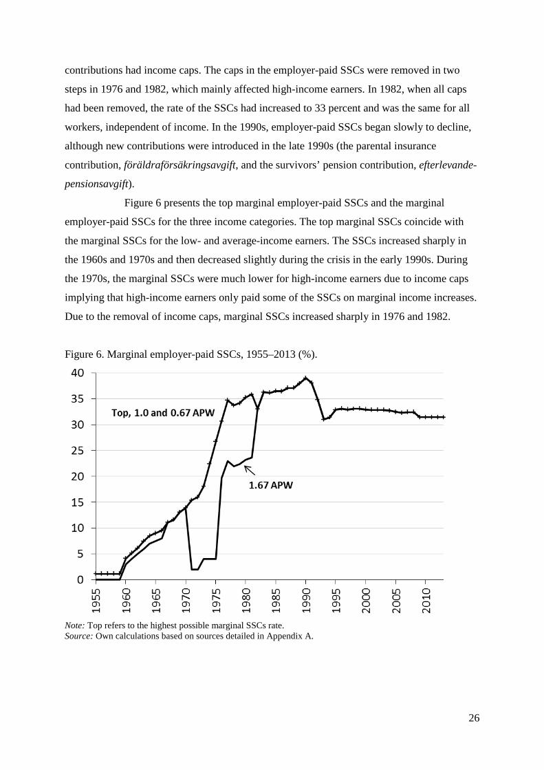
Figure 6 presents the top marginal employer-paid SSCs and the marginal

employer-paid SSCs for the three income categories. The top marginal SSCs coincide with

the marginal SSCs for the low- and average-income earners. The SSCs increased sharply in

the 1960s and 1970s and then decreased slightly during the crisis in the early 1990s. During

the 1970s, the marginal SSCs were much lower for high-income earners due to income caps

implying that high-income earners only paid some of the SSCs on marginal income increases.

Due to the removal of income caps, marginal SSCs increased sharply in 1976 and 1982.

Figure 6. Marginal employer-paid SSCs, 1955–2013 (%).

Note: Top refers to the highest possible marginal SSCs rate. Source: Own calculations based on sources detailed in Appendix A.

27

4. The marginal tax wedge on labor income We now present the development of the marginal tax wedge on labor income, that is, the

combined marginal effect of all the taxes described above. The marginal tax wedge is

presented for the three income levels and the income level at which the top marginal tax

wedge begins to be applied. Figure 7 depicts the marginal tax wedge for our three categories

and the top marginal tax wedge between 1862 and 2013 (excluding consumption taxes).

Figures 8a, 8b and 8c depict the top marginal tax wedge and the income level at which the top

marginal tax wedge begins to be applied. Figure 9 depicts the marginal tax wedge, including

consumption taxes.

Figure 7. Marginal tax wedges on labor income, 1862–2013 (%).

Note: In the early 1970s, the tax wedge of the average-income earner is higher than that of the high-income earner due to the much lower marginal SSCs paid by the high-income earner. In the late 1990s, the tax wedge of the low-income earner is higher than that of the average-income earner, as the low-income earner’s basic allowance decreases as income increases, which affects the marginal tax rate for the low-income earner. Source: Own calculations based on sources detailed in Appendix A.

4.1 The marginal tax wedge for the low-, average- and high-income earner

Figure 7 shows that the marginal tax wedges for the examined income categories were all

approximately three percent in 1862. At the turn of the twentieth century, these wedges had

increased to approximately five percent. The main explanation was higher local taxes.

Nonetheless, the marginal tax wedges were low compared with future levels.

28

Until the 1920 tax reform, the marginal tax wedges increased only slightly for

the three income categories. Although the state income tax schedule was progressive, the

marginal tax wedges were about the same because progressivity did not set in until higher

levels of income. The defense taxes during World War I did not affect our three income

categories.

At the beginning of the 1920s, the marginal tax wedges began to increase due to

the new state tax system and increasing local taxes. The wedges oscillated around 12 percent.

Nevertheless, there were no major differences in the wedges across the three categories.

During the Depression, the introduction of temporary taxes and the ordinary tax rate increases

led to marginal tax wedge increases. The marginal tax wedges did not decline after the

Depression, and the wedges were approximately 15 percent in 1938.

Along with the 1939 tax reform, new temporary defense taxes further increased

the marginal tax wedges. At this point, the wedges of the three income categories began to

diverge slightly. At the end of the war, the marginal tax wedge was between 20 and 25

percent. The increase was driven by the changes in the state income tax system. The

combined effect of the new tax system in 1939 and the defense taxes was large for the state

marginal income tax rate. Compared to ten years before, the state marginal income tax rate

had almost tripled for the low-income earner and more than tripled for the high-income earner

by 1947. In addition to higher formal tax rates, the progressive nominal tax schedule, high

inflation and high wage increases automatically increased marginal income tax rates during

World War II.

The wedge increases were made permanent after World War II, when the

defense taxes were abolished and a new tax system was introduced. The marginal tax wedge

had roughly doubled in 20 years. After World War II, the marginal tax wedge continued to

increase. In 1960, the marginal tax wedge was approximately 35 percent for the low-income

earner and slightly and well above 40 percent for the average- and high-income earners,

respectively. The driving force behind this sharp increase was, again, price and wage inflation

and the highly progressive tax schedule introduced in 1948, which pushed taxpayers into

higher tax brackets with higher marginal income tax rates. This inflation-driven tax increase

mechanism implied that Parliament did not have to pass new tax laws to increase tax rates and

tax revenue.

In the 1960s, this development continued, but the marginal tax wedge increases

were also a result of increasing SSCs. In 1970, the marginal tax wedges were approximately

29

50, 55 and 60 percent, respectively, for the three income categories. The marginal tax wedge

had again doubled over a 20-year period.

In 1971, efforts to redistribute income culminated in the implementation of a

new tax reform. The progressivity of the income tax was strengthened. Later, the so-called

“Haga policy” of the 1970s attempted to dampen marginal income tax rate increases.

However, even when the statutory state marginal income tax rates were reduced, particularly

for low- and average-income earners, the local income tax rates and, in particular, the SSCs

continued to increase. Moreover, the local tax was no longer deductible. In tandem with this

development, inflation accelerated during the 1970s, which led to increased bracket creep. As

a result, the marginal tax wedge continued to increase for the high-income earner but

fluctuated for the low- and average-income earners. Around 1980, the wedges were

approximately 60, 70 and 85 percent, respectively, for the three income levels analyzed.

Marginal tax wedges had thus tripled in 40 years.

The 1983–1985 tax reform reduced the marginal tax wedge for all three income

categories by 5–10 percentage points, whereas it fluctuated for the remainder of the 1980s.

The 1990–1991 tax reform decreased marginal tax wedges by 10–15 percentage points. At the

end of the period examined, the marginal tax wedge was approximately 46 percent for the

low-income earner, approximately 48 percent for the average-income earners and

approximately 63 percent for the high-income earner.

4.2. The top marginal tax wedge

In addition to the marginal tax wedge at three income levels, the evolution of the top marginal

tax wedge over time also commands our attention.

To prevent extreme tax rates, tax caps have occasionally been introduced.

Average tax caps were in place between 1903 and 1938 on the state income tax and between

1920 and 1938 on the local progressive tax. These tax caps reduced the marginal tax rates on

very high incomes, which implied that the top marginal tax rate did not apply to the highest

income levels. An explicit marginal tax rate cap was in place between 1980 and 1987 for the

marginal tax rate (including both the state and the local taxes). This cap directly reduced the

top marginal tax rate and tax wedge.37

Figure 7 shows that the top marginal tax wedge was low during the nineteenth

century and the early twentieth century compared with later levels. During World War I, the

37 There were also tax caps that restricted the sum of wealth and income taxes (see Du Rietz and Henrekson 2015).

30

top wedge rose sharply. The postwar tax reform and the introduction of a local progressive tax

meant that the top marginal tax wedge increased from about ten percent to 35 percent in 20

years. About half of the effect can be attributed to the state marginal tax rate.

During the 1920s, the top marginal tax wedge decreased slightly when the

economy was booming. During the 1930s and the Depression, new taxes were imposed and

ordinary tax rates increased. As a result, the top marginal tax wedge increased again to almost

50 percent.

The top marginal tax wedge continued to increase after the Depression to more

than 70 percent during World War II. The increase was mainly caused by supposedly

temporary tax increases to strengthen military capacity. However, this level was maintained

after the war and throughout subsequent decades. The top marginal tax wedge increased

slowly due to increasing local taxes and slowly increasing SSCs. However, the top marginal

tax wedge was slightly reduced in 1953, when the top marginal state tax rate was lowered. In

the 1970s, the top marginal tax wedge again increased more sharply due to increased income

taxes and increased employer-paid SSCs. The top marginal tax wedge peaked at almost 90

percent at the end of the 1970s.

The top marginal tax wedge was slightly reduced due to the marginal tax cap

and the tax reform in the first half of the 1980s. However, it was not until the major 1990–

1991 tax reform that the top marginal tax wedge substantially decreased to approximately 65

percent. Since that reform, the top marginal tax wedge has slightly increased. In 2013, the top

marginal tax wedge was at the same level as it was at the beginning of World War II.

The top marginal tax wedge has often been substantially higher than the

marginal tax wedge for the high-income earners (1.67 APW). The figures begin to deviate at

the beginning of the twentieth century with the new tax system. Nonetheless, the top marginal

tax wedge was moderate at that time compared with later levels. The marginal tax wedge paid

by the high-income earners deviated sharply from the top marginal tax wedge between the

wars. At the end of the 1930s, the top marginal tax wedge was almost 50 percent, whereas the

marginal tax wedge of the high-income earner was less than half that value.

After World War II, high inflation and bracket creep pushed all three types of

income earners closer to the top marginal tax rate. Around 1980, the tax wedge of the high-

income earner peaked at close to 90 percent. By the end of the 1980s, the formal top marginal

tax wedge coincided with the actual marginal tax wedge of the high-income earner at

approximately 80 percent, and these figures continued to roughly coincide during the

remainder of the period.

31

The evolution clearly shows how temporary tax increases during the World

Wars and depressions, are made permanent after the crises. The top marginal tax wedge

increased stepwise until the beginning of the 1980s and then decreased.38 The early

development supports the idea that the acceptable burden of taxation increases during crises

and the acceptance of a higher tax level remains following the crises, leading to a stepwise

increasing function of tax rates.39 The sharp decrease in marginal tax wedges after the tax

reform at the beginning of the 1990s represents a break from this pattern.

4.3. The relative top tax income threshold

Considering the income at which the top marginal tax wedge begins to be applied can further

extend this analysis. To make this income comparable over time, some form of relative

income level should be calculated. Thus, we compute the relative top tax income threshold,

which is defined as the wage at which the top marginal tax wedge begins to be applied,

divided by the APW. The results are presented in Figures 8a–8c.

Before 1903, the income tax was proportional, and we do not report any figures

before this year. When the progressive income tax system was introduced in 1903, the relative

top tax income threshold was approximately 100 APWs. The top marginal tax rate was

slightly more than ten percent at that time.

Ignoring the defense taxes during World War I, which almost tripled the relative

top tax income threshold, the threshold decreased slowly until the 1920 tax reform. With the

tax reform in 1920, the top marginal wedge increased to 35 percent, and this wedge initially

applied to incomes above almost 400 APWs. The nominal income at which a taxpayer had to

begin paying top marginal tax rates was unchanged between the World Wars, but the

threshold normally fluctuated between 450 and 550 APWs due to changing wages (including

wage cuts).

The 1939 tax reform and the defense tax increased the top marginal tax wedge

to almost 60 percent at the same time as the threshold decreased to less than 100 APWs,

which was the largest decrease during the entire period. Due to increasing wages, the

threshold continued to fall during World War II. In 1948, the threshold was almost halved 38 This stepwise pattern is more pronounced during the first half of the period examined. After World War II, the development may be described as a slow increase in the 1950s and the 1960s and a more rapid increase in the 1970s. 39 The idea was originally put forward by Peacock and Wiseman (1961). Higgs (1987) shows that economic crises and wars may explain (part of) the increase of federal expenditures in the U.S. during the twentieth century. Rodriguez (1980) also argues that the Swedish evolution supports this idea. However, the hypothesis is difficult to formally test and empirical support analyzing the evolution of public spending during, for instance, World War II is inconclusive (Henrekson 1993).

32

compared with 1939. However, the top marginal tax wedge continued to increase to

approximately 70 percent due to high defense taxes during World War II. The tax reform did

not imply any major changes. The temporary increase of the marginal tax wedges was made

permanent and the income at which the top marginal tax wedge begins to be applied, was

about the same.

Although the top marginal tax wedge did not change much until the 1970s, the

threshold continued to fall, mainly due to nominal wage increases. In 1970, it had decreased

to seven APWs from approximately 40 in 1948.40 This development continued during the

1970s, at the same time as the top marginal income tax wedge began to increase again. In

1979, the year before the marginal tax cap was introduced, the top marginal income tax wedge

was almost 90 percent, and the threshold was 2.6 APWs. Since the end of the 1980s, the

threshold has been below two.

Hence, during the period examined, the threshold decreased from at most nearly

600 APWs in the 1920s to less than two in the late 1990s. Analyzing the top marginal tax

wedge only gives half of the story, as it does not say anything about the income level at which

it begins to be applied. It is true that the top marginal income tax rate did not change much

during the 1950s and 1960s, but the threshold decreased significantly, pushing more people

into the highest tax bracket.

40 The slightly lowered top marginal income tax rate in 1953 was associated with a sharp decrease in nominal income when the tax was applied. The threshold declined from 34 to 20 APWs in this year alone.

33

Figure 8a. The top marginal tax wedge and the relative top tax income threshold, 1903–2013.

Note: The right scale refers to the marginal tax wedge (%), and the left scale refers to the relative top tax income threshold, which is expressed as the number of APWs at which the top marginal tax wedge begins to be applied. Source: Own calculations based on sources detailed in Appendix A. Figure 8b. The top marginal tax wedge and the relative top tax income threshold, 1939–2013.

Note: The scale refers both to the marginal tax wedge (%) and the relative top tax income threshold, which is expressed as the number of APWs at which the top marginal tax wedge begins to be applied. Source: Own calculations based on sources detailed in Appendix A.

34

Figure 8c. The top marginal tax wedge and the relative top tax income threshold, 1970–2013.

Note: The right scale refers to the marginal tax wedge (%), and the left scale refers to the relative top tax income threshold, which is expressed as the number of APWs at which the top marginal tax wedge begins to be applied. Source: Own calculations based on sources detailed in Appendix A.

4.4 The marginal tax wedges including consumption taxes

In Section 4.1, we excluded consumption taxes when we calculated the marginal tax wedge;

in this section, we will show the evolution of the marginal tax wedge when consumption taxes

are taken into account. We have computed consumption taxes as the sum of value-added

taxes, sales taxes, all specific consumption taxes and excise duties (including energy and

environmental taxes), divided by total private consumption.

Including consumption taxes, the average-income earner’s tax wedge increases

by five to ten percentage points until the beginning of the 1990s and between ten and 15

percentage points by the end of the period (see Figure 9). The difference is somewhat higher

for the low-income earner and somewhat lower for the high-income earner and for the top

marginal tax wedge.41

41 See Stenkula (2015) for further details regarding consumption taxes.

35

Figure 9. Marginal tax wedges on labor income, including consumption taxes, 1862–2013 (%).

Note: In the early 1970s, the average-income earner’s tax wedge is higher than that of the high-income earner, as a result of much lower marginal SSCs paid by the high-income earner. In the late 1990s, the low-income earner’s tax wedge is higher than that of the average-income earner because the low-income earner’s basic allowance decreases as income increases, which affects the marginal tax rate for the low-income earner. Source: Own calculations based on sources detailed in Appendix A.

4.5 Discussion

The analysis shows that there are distinct periods with certain features, which are

distinguishable from other periods and separated by turning points caused by major tax

reforms that represent a break with previous periods. The evolution might broadly be divided

into five separate periods.

The first period stretches from 1862 until World War I. Marginal tax wedges

were low and slowly increasing. The income tax was also proportional until the 1903 tax

reform and only slightly progressive until World War I. The second period stretches from

World War I and the 1920 tax reform until World War II, in which the marginal tax wedges

increased. In particular, the top marginal tax wedge increased sharply. Although the

progressivity was higher, the tax brackets were wide, and most taxpayers were situated in the

lowest tax bracket, which led to a less pronounced marginal tax wedge increase.

A high top marginal tax wedge, along with increasing tax wedgeswhich

became very high for “ordinary” taxpayerscharacterizes the third period, after World War II

36

until the 1971 tax reform. The tax system had a distinct progressive feature with an explicit

distributional purpose, beginning with the tax reform implemented in 1948. Although there

were no more substantial increases in the top marginal tax wedge until the tax reform

implemented in 1971, the income level where the top marginal tax wedge began to be applied

dropped sharply. This threshold declined from more than 400 APWs just before World War II

to seven APWs by 1970.

The fourth period begins with the 1971 tax reform, in which efforts to

redistribute income culminated (Elvander 1972; Lindbeck 1997; Lodin 2011), and lasts until

“the tax reform of the century” in 1990–1991. This period is distinguished by the highest tax

wedges of the entire period (1862–2013). Tax wedges peaked around 1980 when the top

marginal tax wedge and the marginal tax wedge for the high-income earner could reach 90

percent. Employer-paid SSCs were sharply increased. Taxpayers were increasingly subject to

the top marginal tax wedge, as the relative top tax income threshold continued to drop until an

income of less than two APWs was enough to pay the top marginal tax wedge.

The major tax reform in 1990–1991 decreased the marginal tax wedges to levels that

prevailed before the fourth period. This reform was the starting point for the fifth period,

which was characterized by falling tax wedges.

5. Conclusions

The effect of marginal taxes on economic behavior and economic development has attracted

great interest from researchers and policymakers because marginal taxes influence, among

other things, the supply of hours, effort at work, taxable income, occupational choice, career

aspirations and educational effort. A wider measure, such as the marginal tax wedge, often

better captures the combined effect from different taxes on individual choices than a measure

that studies the effect of one narrow form of taxation, such as the marginal tax rate. Therefore,

a wider measure is often preferable. The analysis may also benefit from a longer time

perspective, as tax systems may change slowly, and it may take a long timesometimes

generationsbefore all effects are played out.

In this paper, we have derived a homogenous series of marginal tax wedges on

labor income in Sweden. We have compiled information on the tax system and computed tax

wedges for more than 150 years of tax history (1862–2013). We are interested in determining

whether the evolution of tax wedges reveals periods with different characteristics and whether

turning points in Swedish tax history are detectable.

37

Following the OECD, we have calculated marginal tax wedges for low-,

average- and high-income earners. We have also computed the top marginal tax wedge on

labor and the income at which the top marginal tax wedge begins to be applied. These data

and analyses are unique: no one has thus far calculated this for Sweden. Moreover, we also do

not know of a corresponding study for any other country.

The analysis shows that marginal tax wedges were low and about the same for a

low-, average- and high-income worker until the 1920 tax reform, although progressivity was

previously introduced in the 1903 tax reform. The top marginal tax wedge increased

considerably during World War I and increased further during the Depression in the 1930s.

The wedges rose sharply through temporary defense taxes during World War II, which were

made permanent by the 1948 tax reform. The marginal tax wedges for the three income

categories continued to increase thereafter, mainly as the result of increased local government

taxes, the introduction and increase of employer-paid SSCs and bracket creep, that is, as a

result of inflation, whichtogether with a progressive tax schedulepushed taxpayers into

tax brackets with higher marginal tax rates. The income when the top marginal tax wedge

began to be applied decreased sharply during this period. It required close to 500 APWs to be

subject to the top marginal tax in 1938, about seven APWs in 1970 and a mere 1.6 APWs by

the end of the 1980s. The wedges peaked around 1980. At this point, the high-income earner

began to pay the top marginal tax wedge, which could be as high as 90 percent. The major tax

reform in 1990–1991 lowered the tax wedges to levels that matched pre-1971 levels (before

the 1971 tax reform). In 2013, the final year of the study, the top marginal tax wedge was

approximately 67 percent, which mirrored the 1941–1942 level.

The evolution can be divided into five distinct periods. During the first period,

from 1862 until World War I, the income tax system was largely proportional and featured

low and slowly increasing tax wedges. In the second period, during the interwar period, the

tax wedges, particularly the top marginal tax wedge, increased. The third period, stretching

from the 1948 tax reform until the 1971 tax reform, was characterized by steadily increasing

tax wedges and a more progressive income tax system. The 1971 tax reform constitutes the

beginning of the fourth period, during which efforts to redistribute income culminated and the

tax wedges were peaking. The 1990–1991 tax reform represents the beginning of the final and

ongoing period with decreasing marginal tax wedges.

Notably, the periods we identify largely coincide with the categorization of the

Swedish economic system into the four “models” of Swedish economist Assar Lindbeck

(Lindbeck 2012, 342–359): the market-oriented period (1870–1939), the welfare capitalism

38

period (1945–1970), the interventionist period (1970–1990) and the partial liberalization

period (starting in 1990).42 It is conceivable that the same ideologies, economic theories and

structural changes underlying tax reforms and tax policy also affect other policy areas. Our

time series can be used in future research to study the conjecture that tax policy coevolves

with other policies, such as labor market policy and monetary policy. A further step might be

taken to relate taxation and other economic policy areas to economic outcomes, such as

employment, structural change, the size distribution of firms and economic growth.

42 Our first two periods coincide with the first period in Lindbeck’s classification.

39

Appendix A. Sources. Information regarding the marginal income tax rates during the appropriation system was

collected from SFS 1861:34, SFS 1871:30, SFS 1879:25, SFS 1880:46, SFS 1881:29, SFS

1883:51, SFS 1892:44, SFS 1892:111, SFS 1893:34, SFS 1894:76, SFS 1895:62, SFS

1897:111, SFS 1901:31, SFS 1901:34, SFS 1902:50, SFS 1910:116, SFS 1920:759, Eberstein

(1929, 119–135), Eberstein (1937, 694–695), Genberg (1942, 4–5, 18) and Gårestad (1987,

38–40).

Data on the marginal income tax rates from the 1903 tax reform onwards were

collected from SFS 1902:84, SFS 1910:115, SFS 1917:513, SFS 1918:512–513, Genberg

(1942), Söderberg (1996) and OECD stats extracts, Taxing Wages.43

Statistics on local taxes are incomplete before 1875 (Gårestad 1987, 197, 213–

215). We impute a tax rate of two percent between 1862 and 1874, which is slightly below the

estimated tax level in 1875. For 1875–1914, Gårestad (1987, 212–213, Table 4) has compiled

information regarding the total amount of various income taxes paid to local governments.

For this period, we estimate the tax rate as total income taxes paid to the municipalities

(excluding local lump-sum taxes), divided by total labor income earned by the taxpayers, as

reported by Edvinsson (2005, 385–388). For 1915–1920, we base our estimate on Rodriguez

(1981, 107–108) and Edvinsson (2005, 385–388). After 1920, the marginal local tax rate is

found using the available statutory tax rates reported in Söderberg (1996, 63–64) and

Statistics Sweden.44 Because the tax rates differ among cities, the average local tax rate was

used. Until 1952, a tax earmarked for the national church was mandatory and included in the

local tax.45 After 1952, this tax was not levied on taxpayers who had left the national church.

Since 2000, the national church has been separate from the government, and the fee to the

national church is no longer regarded as a tax (Skatteverket 2000, 56). In our time series, we

follow the OECD and exclude the national church tax beginning in 2000.46

The income tax system also includes tax relief in the form of allowances and tax

credits, where allowances are applied to pre-tax income to obtain taxable income. Basic local 43 See http://stats.oecd.org/Index.aspx?DataSetCode=AWCOMP http://stats.oecd.org/Index.aspx?DataSetCode=AWCOMP_OLD http://stats.oecd.org/Index.aspx?DataSetCode=AWHIST_OLD 44 See http://www.scb.se/sv_/Hitta-statistik/Statistik-efter-amne/Offentlig-ekonomi-/Finanser-for-den-kommunala-sektorn/Kommunalskatterna/11849/11856/67892/ 45 Tithes had to be paid to the church earlier in history. In reforms carried out in 1527 by King Gustav Vasa, part of the tithe was abolished, part was converted to a central state tax and the remaining part was later transformed into a local tax (Eberstein 1937, 822–832). 46 The formal tax rate differed somewhat between parishes. In 1953, the national church tax was about 0.80 percent on average. In 2013, there was a compulsory fee for a funeral service, averaging 0.22 percent. The voluntary fee to the church was 1.01 percent on average (Skatteverket 2013, 137).

40

and state income tax allowances were introduced in 1920 (Söderberg 1996, 2). The basic tax

allowances differed somewhat among cities until 1960, depending on the price level in each

city. We refer to the average city when calculating the basic tax allowance. Information is

gathered from Genberg (1942), Söderberg (1996), Skattebetalarnas förening (1997) and

Skatteverket (1998–2013). The local tax was also deductible from the state taxable income

between 1920 and 1970. The basic state and local income tax allowances may positively or

negatively affect the marginal income tax rate because these allowances occasionally depend

on and change with income level. Information regarding tax credits for the 1999–2002 period

and for the 2007–2013 period was gathered from Skatteverket (2002, 50) and Ministry of

Finance (2006–2012), respectively.

Information about employee-paid social security contributions was collected

from Elmér (1960), Söderberg (1996) and Skatteverket (1998–2013), and information about

employer-paid social security contributions was collected from Söderberg (1996, 117–119)

and Skatteverket (2013, 144, Table 7.32).

Information about consumption taxes was collected from Statistics Sweden

(1914–2011) and Ekonomistyrningsverket (2010–2014), whereas information about private

consumption was retrieved from Edvinsson (2005, 322–326) and Statistics Sweden.47

47 Consumption taken from Annual estimates, National Accounts, http://www.scb.se/en_/Finding-statistics/Statistics-by-subject-area/National-Accounts/.

41

Appendix B. Extensions. We have followed the approach by the OECD and included income taxes and social security

contributions (SSCs) in the marginal tax wedges. We have also calculated the marginal tax

wedge with and without consumption taxes. In line with the OECD, the SSCs have been

treated as a pure tax. In this appendix, we show the evolution of the marginal tax wedge when

the benefit component of social security contributions is taken into account and how this

evolution differs from our calculations in the main text. In addition, we report the effects of

marriage and joint taxation.

Accounting for the benefit component of the SSCs

The OECD treats all SSCs as taxes. Heady (2004) claims that all SSCs should be treated as

taxes because they are compulsory and unrequited payments to the government. Although

there might be some link between contributions and benefits, country comparisons should

treat SSCs as a tax because the country choice between general taxes and earmarked

compulsory contribution should not alter the comparison. McKee, Visser and Saunders (1986)

further argue that the perceived relationship between incremental contributions and

incremental benefits is likely weak when the contributions are compulsory. Moreover, it is

difficult to estimate the benefit component of the SSCs. Most researchers also ignore the

benefit components and treat social security contributions as pure taxes. However, Disney,

Boeri and Jappelli (2004) and Disney (2006) argue that it is important to adjust the SSCs for

the benefit component. In their view, a description and analysis of the tax system without

these adjustments will be skewed and will then yield an incorrect picture of actual taxes.

Comparison over time within a country should thus include an adjustment for the benefit

component.

Employer-paid SSCs were introduced in 1955. We apply the estimates used by,

for instance, SOU (SOU 1989:33, 61–63), that three-quarters of the employer-paid marginal

SSCs were initially taxes.48 Since 1987, the high-income earner’s wage has exceeded the

benefit caps; hence, the marginal tax effect is 100 percent. Since 2000, 60 percent of the

employer contributions have been regarded as taxes for the low- and average-income earner.

The decreased tax share is a result of pension contributions becoming more actuarial, that is,

the connection between contributions paid and benefits received was higher (Skatteverket

1998, 46). 48 SOU (Statens offentliga utredningar) is the Swedish official series of reports of committees appointed by the Swedish Government.

42

The first employee-paid SSC, the national basic pension contribution,

introduced in 1913, corresponded fully to a benefit until 1935. The benefit share was

gradually reduced beginning in 1936, and from 1948 until 1973 (when it was abolished), the

national basic pension contribution was a tax (Elmér 1960, 222). The second employee-paid

SSC, the sick leave benefit fee, introduced in 1955, is estimated to have a benefit share of 50

percent in 1974 (the same year as it was abolished) because there was some connection

between the contribution and benefit. For the other years, this SSC had no benefit share. In

1993, employee-paid SSCs were reintroduced and were called general SSCs. In effect, they

were pure taxes.49

Adjustments for the estimated benefit component had no discernible effect on

the tax wedge until the 1970s. The marginal tax wedge decreased by seven percentage points

at most at the end of the period examined for the average-income earner (see Figure 10).

Excluding or including the benefit component does not impact the general evolution of the tax

wedge to a large extent, although the explicit tax wedge will certainly be lower when one

adjusts the SSCs for the estimated benefit component. The effect is about the same for the

low-income earner, whereas the effect on the high-income earner is negligible, because,

beginning in 1987, the SSCs give no marginal benefit at an annual income of 1.67 APW.

The marginal tax wedge increases by at most about ten percentage points for the

average-income earner when both consumption taxes and the benefit component of the SSCs

are considered. The effects on low- and high-income earners are similar. For most years, the

long-term evolution for the three income categories remains basically the same. Near the end

of the period examined, the tax wedges are admittedly lower when the benefit component of

the SSCs is adjusted for taxpayers with low incomes, in particular.

49 See, e.g., the discussion in Lewin (2009). Despite that the employee-paid SSCs rate was decreasing (beginning in 2000), the benefits which were supposed to be linked to the contributions were unaffected, implying that the contributions in practice were fiscal.

43

Figure 10. Marginal tax wedge, given different assumptions, for the average-income earner, 1862–2013 (%).

Source: Own calculations based on sources detailed in Appendix A.

Alleviation for married couples

The marginal tax rates and marginal tax wedges calculated thus far have been based on a

single person with no children. However, the tax rates for married couples were more

favorable, partly because they had more generous basic allowances (between 1920 and 1970)

and partly because they had lower tax rates (between 1953 and 1970) for a given taxable

income. Before 1971, married couples were also taxed jointly.

To check the robustness of our results, we have calculated the marginal tax

wedge, given that the taxpayer is married (but assuming that all other assumptions are

unchanged). The results are shown in Figure 11, which shows the evolution for a taxpayer

earning 1.0 APW. There was no effect before World War II. The marginal tax wedge was

lower after World War II, and the tax wedge increase was initially somewhat slower during

the 1950s. It increased more quickly during the 1960s and then caught up with the tax wedge

for unmarried persons after 1971. The long-term evolution for the other two categories is

similar.50

50 To mitigate the effect of separate taxation for families with only one income earner, a small tax reduction was implemented in 1971. This reduction remained in place until 1991.

44

Figure 11. Marginal tax wedge for married and unmarried average-income earners, 1862–2013 (%).

Note: “Married” refers to a couple where one spouse works on the regular labor market with a wage equal to one APW, while the other spouse has no regular income. Source: Own calculations based on sources detailed in Appendix A.

The calculation in Figure 11 refers to a household with one income earner. In

Figure 12, we have, in line with the OECD, calculated the marginal tax wedge for a married

couple, assuming that one spouse is working full time, earning 1.0 APW, and that the other

spouse is working part time, earning 0.33 or 0.67 APW.51 The difference between the

unmarried and two-earner married couple is minor. A couple with a spouse earning 0.67 APW

might occasionally even have a higher marginal tax wedge than an unmarried taxpayer.

51 If both spouses were working, there was also an additional small allowance between 1921 and 1984.

45

Figure 12. Marginal tax wedge for married with working spouse and unmarried average-income earners, 1862–2013 (%).

Note: 0.33 refers to a couple where the principal earner’s income is one APW and the other spouse’s income is 0.33 APW. 0.67 refers to a couple where the principal earner’s income is one APW and the other spouse’s income is 0.67 APW. The figure shows the principal earner’s marginal tax wedge from 1971. Source: Own calculations based on sources detailed in Appendix A.

In Figure 13, we have calculated the marginal tax wedge for a married couple,

assuming that the household head works full time and faces the top marginal tax rate and that

the other spouse earns 0.67 APW. The figure shows the second earner’s marginal tax wedge.

When joint taxation of families was abolished in 1971, the tax wedge decreased

substantiallyfrom over 70 percent to below 50 percent. Even if the principal earner was

facing a higher marginal tax rate after the 1971 tax reform, the second earner received a

decreased tax wedge. This change made it more profitable for women to work and led to an

increasing share of women participating in the labor market.52

52 See, e.g., Gustafsson (1992) for a discussion of female labor participation and wages.

46

Figure 13. Marginal tax wedge, second income earner married to top income earner, 1862–2013 (%).

Note: The figure shows the second income earner’s marginal tax wedge, assuming that the principal earner faces the top marginal tax rate and that the other part earns 0.67 APW. Source: Own calculations based on sources detailed in Appendix A.

47

Appendix C. Results. Table 1. Marginal tax rates and marginal tax wedges, 1862–2013.

Low-income earner (0.67 APW) Average-income earner (1.0 APW) High-income earner (1.67 APW)

Year Wage

Marginal tax rate

%

Marginal Tax wedge

% Wage

Marginal tax rate

%

Marginal tax wedge

% Wage

Marginal tax rate

%

Marginal tax wedge

% 1862 273 2.0 2.0 408 3.0 3.0 681 3.0 3.0 1863 286 2.0 2.0 427 3.0 3.0 713 3.0 3.0 1864 283 2.0 2.0 423 3.0 3.0 706 3.0 3.0 1865 278 2.0 2.0 416 3.0 3.0 694 3.0 3.0 1866 261 2.0 2.0 389 2.0 2.0 650 3.0 3.0 1867 248 2.0 2.0 371 2.0 2.0 619 3.0 3.0 1868 238 2.0 2.0 356 2.0 2.0 594 3.0 3.0 1869 246 2.0 2.0 367 2.0 2.0 613 3.0 3.0 1870 246 2.0 2.0 367 2.0 2.0 613 3.0 3.0 1871 250 2.0 2.0 373 2.0 2.0 623 3.5 3.5 1872 276 2.0 2.0 412 3.0 3.0 688 3.0 3.0 1873 304 2.0 2.0 454 3.0 3.0 757 3.0 3.0 1874 324 2.0 2.0 483 3.0 3.0 807 3.0 3.0 1875 327 2.2 2.2 488 3.2 3.2 814 3.2 3.2 1876 323 2.5 2.5 482 3.5 3.5 805 3.5 3.5 1877 332 2.6 2.6 495 3.6 3.6 827 3.6 3.6 1878 300 3.0 3.0 447 4.0 4.0 747 4.0 4.0 1879 288 3.3 3.3 431 4.8 4.8 719 4.8 4.8 1880 310 3.8 3.8 463 5.3 5.3 773 5.3 5.3 1881 320 3.9 3.9 477 5.4 5.4 797 5.4 5.4 1882 328 4.1 4.1 490 5.6 5.6 819 5.6 5.6 1883 329 4.2 4.2 491 5.2 5.2 819 5.2 5.2 1884 338 4.3 4.3 505 5.3 5.3 844 5.3 5.3 1885 335 4.5 4.5 499 5.5 5.5 834 5.5 5.5 1886 325 4.9 4.9 484 5.9 5.9 809 5.9 5.9 1887 330 4.9 4.9 493 5.9 5.9 823 5.9 5.9 1888 343 4.8 4.8 512 5.8 5.8 856 5.8 5.8 1889 364 4.7 4.7 544 5.7 5.7 908 5.7 5.7 1890 376 4.6 4.6 561 5.6 5.6 936 5.6 5.6 1891 379 4.6 4.6 565 5.6 5.6 944 5.6 5.6 1892 375 4.7 4.7 560 5.7 5.7 936 5.7 5.7 1893 379 4.8 4.8 565 5.8 5.8 944 6.1 6.1 1894 384 4.9 4.9 573 5.9 5.9 957 6.9 6.9 1895 391 4.8 4.8 583 5.8 5.8 974 6.8 6.8 1896 399 4.7 4.7 596 5.7 5.7 996 5.7 5.7 1897 416 4.6 4.6 621 5.6 5.6 1036 5.6 5.6 1898 443 4.5 4.5 662 5.5 5.5 1105 5.5 5.5 1899 464 4.3 4.3 693 5.3 5.3 1157 5.3 5.3 1900 480 4.4 4.4 717 5.4 5.4 1198 5.4 5.4 1901 476 4.8 4.8 710 5.8 5.8 1186 5.8 5.8 1902 482 5.0 5.0 720 6.0 6.0 1202 6.5 6.5 1903 496 5.2 5.2 740 6.2 6.2 1236 7.2 7.2 1904 511 6.2 6.2 762 6.2 6.2 1273 7.2 7.2

48

Low-income earner (0.67 APW) Average-income earner (1.0 APW) High-income earner (1.67 APW)

Year Wage

Marginal tax rate

%

Marginal Tax wedge

% Wage

Marginal tax rate

%

Marginal tax wedge

% Wage

Marginal tax rate

%

Marginal tax wedge

% 1905 518 6.4 6.4 773 6.4 6.4 1291 7.4 7.4 1906 566 6.4 6.4 844 6.4 6.4 1410 7.4 7.4 1907 604 6.4 6.4 901 6.4 6.4 1505 7.4 7.4 1908 605 7.2 7.2 902 7.2 7.2 1507 8.2 8.2 1909 565 7.8 7.8 843 7.8 7.8 1408 8.8 8.8 1910 653 7.3 7.3 975 7.3 7.3 1628 8.3 8.3 1911 661 6.2 6.2 986 6.8 6.8 1647 7.2 7.2 1912 692 6.3 6.3 1033 6.9 6.9 1726 7.5 7.5 1913 711 6.2 6.2 1062 6.8 6.8 1773 7.4 7.4 1914 717 6.5 6.5 1071 7.1 7.1 1788 7.7 7.7 1915 741 7.3 7.3 1105 7.9 7.9 1846 8.5 8.5 1916 837 7.0 7.0 1249 7.4 7.4 2086 8.0 8.0 1917 1006 6.9 6.9 1502 7.3 7.3 2508 7.7 7.7 1918 1376 7.7 7.7 2054 8.1 8.1 3429 8.7 8.7 1919 1724 8.5 8.5 2574 8.7 8.7 4298 9.3 9.3 1920 2015 11.7 11.7 3008 11.8 11.8 5023 11.8 11.8 1921 1816 12.9 12.9 2711 13.0 13.0 4527 13.0 13.0 1922 1419 12.9 12.9 2118 13.0 13.0 3537 13.0 13.0 1923 1364 13.1 13.1 2035 13.2 13.2 3399 13.2 13.2 1924 1417 13.5 13.5 2114 13.5 13.5 3531 13.5 13.5 1925 1449 13.3 13.3 2162 13.4 13.4 3611 13.4 13.4 1926 1466 13.1 13.1 2189 13.2 13.2 3655 13.2 13.2 1927 1475 13.1 13.1 2202 13.2 13.2 3678 13.2 13.2 1928 1477 12.6 12.6 2205 12.7 12.7 3682 12.7 12.7 1929 1549 12.3 12.3 2312 12.3 12.3 3860 12.3 12.3 1930 1553 12.7 12.7 2317 12.7 12.7 3870 12.7 12.7 1931 1491 14.1 14.1 2225 14.1 14.1 3715 14.1 14.1 1932 1426 14.8 14.8 2128 14.8 14.8 3554 14.8 14.8 1933 1430 14.9 14.9 2134 14.9 14.9 3564 14.9 14.9 1934 1492 14.5 14.5 2227 14.5 14.5 3720 14.5 14.5 1935 1533 14.2 14.2 2288 14.2 14.2 3821 14.2 14.2 1936 1555 15.0 15.0 2320 14.2 14.2 3875 14.2 14.2 1937 1628 15.0 15.0 2430 14.2 14.2 4058 14.2 14.2 1938 1697 16.2 16.2 2533 15.4 15.4 4230 15.4 15.4 1939 1775 19.5 19.5 2649 18.7 18.7 4424 18.7 18.7 1940 1893 23.0 23.0 2825 22.2 22.2 4717 24.0 24.0 1941 2035 22.3 22.3 3037 21.5 21.5 5072 23.3 23.3 1942 2236 21.9 21.9 3337 21.9 21.9 5573 24.2 24.2 1943 2381 21.6 21.6 3554 21.6 21.6 5935 23.9 23.9 1944 2490 21.6 21.6 3717 21.6 21.6 6207 23.8 23.8 1945 2622 21.5 21.5 3913 21.5 21.5 6535 23.7 23.7 1946 2865 21.5 21.5 4277 21.5 21.5 7142 23.7 23.7 1947 3255 21.3 21.3 4859 23.6 23.6 8114 25.8 25.8 1948 3572 20.6 20.6 5331 23.2 23.2 8903 26.8 26.8 1949 3930 20.8 20.8 5865 25.3 25.3 9795 28.8 28.8 1950 4104 21.6 21.6 6125 25.1 25.1 10229 28.7 28.7 1951 4848 21.8 21.8 7235 25.3 25.3 12083 31.7 31.7 1952 5671 25.5 25.5 8464 28.1 28.1 14135 36.1 36.1

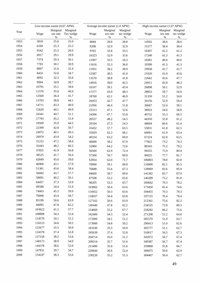
49

Low-income earner (0.67 APW) Average-income earner (1.0 APW) High-income earner (1.67 APW)

Year Wage

Marginal tax rate

%

Marginal Tax wedge

% Wage

Marginal tax rate

%

Marginal tax wedge

% Wage

Marginal tax rate

%

Marginal tax wedge

% 1953 5818 25.0 25.0 8684 28.8 28.8 14502 38.6 38.6 1954 6169 25.3 25.3 9208 32.9 32.9 15377 38.4 38.4 1955 6542 25.2 26.0 9765 32.8 33.5 16307 41.2 41.2 1956 6917 29.1 29.9 10323 32.9 33.6 17240 41.3 41.3 1957 7374 29.3 30.1 11007 33.5 34.3 18381 40.6 40.6 1958 7783 30.1 30.9 11616 35.3 36.0 19399 41.3 41.3 1959 8007 31.6 32.4 11951 38.2 38.9 19958 41.7 41.7 1960 8433 32.0 34.7 12587 38.5 41.0 21020 41.9 43.6 1961 9092 32.3 35.6 13570 38.8 41.8 22662 45.6 47.7 1962 9994 34.9 38.7 14916 39.0 42.5 24911 45.8 48.3 1963 10791 35.1 39.6 16107 39.1 43.4 26898 50.1 52.9 1964 11576 35.9 40.9 17277 43.9 48.3 28853 50.7 54.0 1965 12569 36.4 41.7 18760 42.1 46.9 31330 51.2 54.6 1966 13703 38.8 44.1 20453 42.7 47.7 34156 52.9 56.4 1967 14711 43.3 49.0 21956 46.4 51.8 36667 53.4 58.1 1968 15620 44.1 49.9 23313 47.1 52.6 38933 54.0 58.8 1969 16341 44.7 51.1 24390 47.7 53.8 40732 55.3 60.5 1970 17793 45.2 51.9 26557 48.2 54.5 44350 55.8 61.2 1971 19500 35.9 44.5 29104 47.3 54.3 48604 60.6 61.4 1972 22399 42.8 50.7 33432 57.7 63.5 55831 61.8 62.5 1973 24072 40.1 49.3 35929 62.3 68.1 60001 61.9 63.4 1974 26970 43.9 54.2 40254 63.2 69.9 67224 62.0 63.5 1975 31222 47.2 58.4 46600 58.2 67.0 77822 73.2 74.3 1976 35443 48.2 60.3 52900 64.2 72.6 88343 75.2 79.2 1977 37855 41.9 56.8 56500 62.9 72.4 94355 75.9 80.4 1978 38525 41.7 56.4 57500 59.7 69.9 96025 77.7 81.7 1979 42849 45.0 59.0 63954 62.0 71.7 106803 78.0 82.0 1980 46900 43.1 57.9 70000 59.1 69.8 116900 82.1 85.5 1981 51381 43.6 58.4 76688 55.6 67.3 128069 82.6 85.9 1982 56682 43.7 57.7 84600 58.7 69.0 141282 82.7 87.0 1983 58691 40.2 56.1 87598 53.2 65.6 146289 75.2 81.8 1984 64457 37.3 53.9 96205 53.3 65.7 160662 70.3 78.2 1985 69588 34.4 51.9 103862 50.4 63.6 173450 65.4 74.6 1986 74003 45.3 59.9 110452 50.3 63.6 184455 70.3 78.3 1987 79098 43.4 58.7 118057 50.4 63.8 197155 70.4 78.4 1988 85199 50.6 63.9 127162 50.6 63.9 212361 75.6 82.2 1989 94095 47.8 62.2 140440 47.8 62.2 234535 72.8 80.3 1990 103622 41.2 57.7 154660 55.2 67.7 258282 66.2 75.6 1991 108808 34.3 52.4 162400 34.3 52.4 271208 51.2 64.6 1992 114570 34.1 51.2 171000 34.1 51.2 285570 51.0 63.7 1993 116513 34.8 50.2 173900 34.8 50.2 290413 51.0 62.6 1994 122677 35.5 50.9 183100 35.5 50.9 305777 51.1 62.7 1995 124378 37.4 52.8 185639 37.4 52.8 310017 56.5 67.3 1996 137158 38.2 53.6 204714 35.0 51.2 341872 56.7 67.4 1997 140173 38.9 54.0 209214 35.7 51.6 349387 56.7 67.4 1998 144378 38.6 53.9 215490 35.6 51.6 359868 55.8 66.7 1999 147831 39.7 54.7 220644 36.6 52.4 368475 50.6 62.9 2000 154247 38.3 53.6 230220 35.2 51.3 384467 50.4 62.7

50

Low-income earner (0.67 APW) Average-income earner (1.0 APW) High-income earner (1.67 APW)

Year Wage

Marginal tax rate

%

Marginal Tax wedge

% Wage

Marginal tax rate

%

Marginal tax wedge

% Wage

Marginal tax rate

%

Marginal tax wedge

% 2001 154860 37.2 52.7 231134 34.2 50.4 385994 50.5 62.8 2002 161983 36.0 51.8 241766 32.9 49.5 403749 50.5 62.7 2003 166098 35.5 51.4 247908 35.5 51.4 414006 51.2 63.2 2004 168359 35.9 51.7 251282 35.9 51.7 419641 51.5 63.5 2005 169845 35.4 51.2 253500 35.4 51.2 423345 51.6 63.5 2006 174803 34.8 50.7 260900 34.8 50.7 435703 51.6 63.4 2007 181905 31.6 48.3 271500 31.6 48.3 453405 51.6 63.4 2008 188538 30.4 47.4 281400 30.4 47.4 469938 51.4 63.3 2009 193563 29.5 46.3 288900 29.5 46.3 482463 51.5 63.1 2010 197583 28.6 45.6 294900 28.6 45.6 492483 51.6 63.1 2011 205489 28.6 45.6 306700 28.6 45.6 512189 51.6 63.1 2012 212792 28.6 45.7 317600 28.6 45.7 530392 51.6 63.2 2013 216142 28.7 45.8 322600 31.7 48.1 538742 51.7 63.3

Note: All amounts in the tables refer to SEK. APW = average annual wage of a production worker. The marginal tax rate is the sum of the state and local marginal income tax rates and employee-paid SSCs. Source: Own calculations based on references detailed in Appendix A.

51

Table 2. Top marginal tax rates, top marginal tax wedges and relative top tax income, 1862–2013.

Year

Wage (in thousands)

Relative top tax income threshold

Top state marginal income

tax rate %

Top state marginal income

tax rate* %

Top marginal tax rate

%

Top marginal tax wedge

%

1862 - - 1.0 3.0 3.0 1863 - - 1.0 3.0 3.0 1864 - - 1.0 3.0 3.0 1865 - - 1.0 3.0 3.0 1866 - - 1.0 3.0 3.0 1867 - - 1.0 3.0 3.0 1868 - - 1.0 3.0 3.0 1869 - - 1.0 3.0 3.0 1870 - - 1.0 3.0 3.0 1871 - - 1.5 3.5 3.5 1872 - - 1.0 3.0 3.0 1873 - - 1.0 3.0 3.0 1874 - - 1.0 3.0 3.0 1875 - - 1.0 3.2 3.2 1876 - - 1.0 3.5 3.5 1877 - - 1.0 3.6 3.6 1878 - - 1.0 4.0 4.0 1879 - - 1.5 4.8 4.8 1880 - - 1.5 5.3 5.3 1881 - - 1.5 5.4 5.4 1882 - - 1.5 5.6 5.6 1883 - - 1.0 5.2 5.2 1884 - - 1.0 5.3 5.3 1885 - - 1.0 5.5 5.5 1886 - - 1.0 5.9 5.9 1887 - - 1.0 5.9 5.9 1888 - - 1.0 5.8 5.8 1889 - - 1.0 5.7 5.7 1890 - - 1.0 5.6 5.6 1891 - - 1.0 5.6 5.6 1892 - - 1.0 5.7 5.7 1893 - - 1.3 6.1 6.1 1894 - - 2.0 6.9 6.9 1895 - - 2.0 6.8 6.8 1896 - - 1.3 6.0 6.0 1897 - - 1.0 5.6 5.6 1898 - - 1.0 5.5 5.5 1899 - - 1.0 5.3 5.3 1900 - - 1.0 5.4 5.4 1901 - - 2.0 6.8 6.8 1902 - - 2.0 7.0 7.0 1903 84.4 114 6.0 11.2 11.2 1904 84.4 111 6.0 11.2 11.2 1905 84.5 109 6.0 11.4 11.4 1906 84.5 100 6.0 11.4 11.4 1907 84.6 94 6.0 11.4 11.4

52

Year

Wage (in thousands)

Relative top tax income threshold

Top state marginal income

tax rate %

Top state marginal income

tax rate* %

Top marginal tax rate

%

Top marginal tax wedge

%

1908 85.3 95 6.0 12.2 12.2 1909 85.8 102 6.0 12.8 12.8 1910 85.4 88 6.0 12.3 12.3 1911 85.2 86 6.1 12.2 12.2 1912 85.3 83 6.1 12.3 12.3 1913 239.5 226 19.6 25.7 25.7 1914 85.5 80 6.1 12.5 12.5 1915 86.2 78 6.1 13.3 13.3 1916 85.5 68 6.1 12.6 12.6 1917 85.3 57 6.1 12.3 12.3 1918 966.0 470 23.1 29.9 29.9 1919 969.6 377 23.1 30.3 30.3 1920 1081.8 360 23.4 20.3 33.3 33.3 1921 1089.6 402 26.4 22.8 36.4 36.4 1922 1089.6 514 26.4 22.7 36.5 36.5 1923 1092.2 537 26.4 22.7 36.6 36.6 1924 1096.3 519 26.4 22.6 36.9 36.9 1925 1096.5 507 25.6 21.9 36.2 36.2 1926 1096.9 501 24.1 20.6 35.0 35.0 1927 1096.5 498 24.1 20.6 35.1 35.1 1928 1094.5 496 23.9 20.8 33.8 33.8 1929 1092.4 473 23.0 20.1 32.9 32.9 1930 1097.0 473 23.0 19.9 33.1 33.1 1931 1114.6 501 23.3 19.8 34.5 34.5 1932 1124.5 528 27.3 23.0 38.5 38.5 1933 1118.4 524 30.3 25.7 40.7 40.7 1934 1111.2 499 32.5 27.8 42.2 42.2 1935 1106.9 484 32.5 27.9 42.0 42.0 1936 1107.3 477 36.5 31.4 45.4 45.4 1937 1107.3 456 36.5 31.4 45.4 45.4 1938 1117.7 441 38.0 32.3 47.3 47.3 1939 226.0 85 53.7 47.5 59.0 59.0 1940 226.9 80 60.8 53.5 65.4 65.4 1941 224.9 74 60.8 54.0 65.1 65.1 1942 223.5 67 68.8 61.5 72.0 72.0 1943 222.6 63 68.8 61.8 71.9 71.9 1944 222.4 60 68.8 61.8 71.9 71.9 1945 222.2 57 68.8 61.9 71.9 71.9 1946 222.2 52 68.8 61.9 71.9 71.9 1947 221.7 46 68.8 62.0 71.8 71.8 1948 221.8 42 70 63.1 72.9 72.9 1949 222.5 38 70 62.9 73.0 73.0 1950 222.1 36 70 63.0 73.0 73.0 1951 222.7 31 70 62.9 73.1 73.1 1952 285.8 34 70 61.2 73.8 73.8 1953 174.0 20 65 56.7 69.5 69.5 1954 173.3 19 65 56.9 69.3 69.3 1955 173.0 18 65 57.0 69.3 69.3

53

Year

Wage (in thousands)

Relative top tax income threshold

Top state marginal income

tax rate %

Top state marginal income

tax rate* %

Top marginal tax rate

%

Top marginal tax wedge

%

1956 173.3 17 65 57.0 69.3 69.3 1957 173.7 16 65 56.8 69.4 69.4 1958 175.9 15 65 56.1 69.8 69.8 1959 177.0 15 65 55.8 70.0 70.0 1960 177.9 14 65 55.5 70.1 70.1 1961 178.6 13 65 55.3 70.3 70.3 1962 179.6 12 65 55.1 70.3 70.3 1963 180.1 11 65 55.0 70.4 70.4 1964 182.3 11 65 54.3 70.8 70.8 1965 184.0 9.8 65 53.8 71.0 71.0 1966 186.3 9.1 65 53.1 71.4 71.4 1967 187.3 8.5 65 52.8 71.5 71.5 1968 188.8 8.1 65 52.4 71.8 71.8 1969 190.9 7.8 65 51.8 72.1 72.4 1970 192.7 7.3 65 51.4 72.4 72.6 1971 150.0 5.2 54 76.5 77.0 1972 150.0 4.5 54 77.8 78.2 1973 150.0 4.2 54 77.9 78.8 1974 150.0 3.7 54 78.0 78.9 1975 154.5 3.3 56 81.2 82.0 1976 154.5 2.9 57 83.2 85.9 1977 154.5 2.7 58 84.9 87.7 1978 154.5 2.7 58 86.7 89.1 1979 166.5 2.6 58 87.0 89.4 1980 174.0 2.5 58 85.0 87.8 1981 192.0 2.5 58 85.0 87.9 1982 207.0 2.4 58 85.0 88.7 1983 328.5 3.8 54 84.0 88.3 1984 342.0 3.6 52 82.0 86.8 1985 351.0 3.4 50 80.0 85.3 1986 351.0 3.2 50 80.3 85.6 1987 351.0 3.0 47 77.4 83.5 1988 200.0 1.6 45 75.6 82.2 1989 200.0 1.4 42 72.8 80.3 1990 200.0 1.3 35 66.2 75.6 1991 180.3 1.1 20 51.2 64.6 1992 197.3 1.2 20 51.0 63.7 1993 204.1 1.2 20 51.0 62.6 1994 203.8 1.1 20 51.1 62.7 1995 223.4 1.2 25 56.5 67.3 1996 231.1 1.1 25 56.7 67.4 1997 234.3 1.1 25 56.7 67.4 1998 242.7 1.1 25 56.7 67.4 1999 389.5 1.8 25 56.5 67.3 2000 398.5 1.7 25 55.4 66.4 2001 411.1 1.8 25 55.5 66.5 2002 430.9 1.8 25 55.5 66.5 2003 447.2 1.8 25 56.2 67.0

54

Year

Wage (in thousands)

Relative top tax income threshold

Top state marginal income

tax rate %

Top state marginal income

tax rate* %

Top marginal tax rate

%

Top marginal tax wedge

%

2004 458.9 1.8 25 56.5 67.2 2005 465.2 1.8 25 56.6 67.2 2006 472.3 1.8 25 56.6 67.2 2007 488.6 1.8 25 56.6 67.2 2008 507.1 1.8 25 56.4 67.1 2009 538.8 1.9 25 56.5 66.9 2010 545.2 1.8 25 56.6 66.9 2011 560.9 1.8 25 56.6 66.9 2012 587.2 1.8 25 56.6 67.0 2013 604.7 1.9 25 56.7 67.1

Note: The relative top tax income threshold is defined as the income at which the top marginal tax wedge begins to be applied, divided by the APW. This series stretches from 1903 to 2013 because the income tax system was proportional before 1903. An average tax cap that reduced the marginal tax rates on very high income levels was in place in some years, that is, the top marginal tax rate was paid between an interval where we present the lower bound. * The top state marginal income tax rate includes the effect from the deductible local taxes in 1920–1970. Source: Own calculations based on references detailed in Appendix A.

55

Appendix D. Tax tables. Table 3. The local tax rate and the consumption tax rate, 1862–2013.

Year Local tax Consumption tax Year Local tax Consumption tax % % % %

1862 2.0 3.1 1907 5.44 4.7 1863 2.0 3.3 1908 6.20 4.9 1864 2.0 3.5 1909 6.81 4.3 1865 2.0 3.7 1910 6.34 4.7 1866 2.0 3.5 1911 6.15 4.9 1867 2.0 2.9 1912 6.21 4.8 1868 2.0 3.1 1913 6.07 4.6 1869 2.0 3.1 1914 6.38 4.3 1870 2.0 3.6 1915 7.15 3.9 1871 2.0 4.1 1916 6.46 3.7 1872 2.0 3.9 1917 6.19 2.1 1873 2.0 4.1 1918 6.83 1.4 1874 2.0 4.2 1919 7.18 2.2 1875 2.18 4.0 1920 7.39 2.8 1876 2.51 4.1 1921 8.52 3.7 1877 2.60 3.9 1922 8.57 4.5 1878 3.05 4.0 1923 8.79 5.3 1879 3.29 4.1 1924 9.13 5.5 1880 3.76 4.5 1925 9.15 5.2 1881 3.93 4.5 1926 9.18 5.4 1882 4.13 4.4 1927 9.17 5.6 1883 4.21 4.3 1928 9.02 5.5 1884 4.33 4.5 1929 8.84 5.7 1885 4.52 4.5 1930 9.23 5.6 1886 4.88 4.9 1931 10.67 5.7 1887 4.86 4.3 1932 11.46 6.4 1888 4.78 5.3 1933 10.97 6.6 1889 4.66 5.2 1934 10.39 7.1 1890 4.64 5.3 1935 10.04 7.3 1891 4.60 5.0 1936 10.08 7.4 1892 4.74 4.6 1937 10.08 7.5 1893 4.84 4.9 1938 10.53 8.0 1894 4.94 5.1 1939 11.51 8.6 1895 4.84 5.4 1940 11.87 8.1 1896 4.73 5.6 1941 11.09 8.8 1897 4.62 5.7 1942 10.53 10.3 1898 4.47 5.5 1943 10.17 10.7 1899 4.33 5.5 1944 10.09 10.6 1900 4.44 5.5 1945 10.00 13.0 1901 4.76 5.3 1946 10.00 12.2 1902 5.05 5.0 1947 9.80 10.6 1903 5.17 5.1 1948 9.83 11.6 1904 5.21 5.3 1949 10.12 11.2 1905 5.37 5.5 1950 9.97 10.6 1906 5.36 4.6 1951 10.19 10.6

56

Year Local tax Consumption tax Year Local tax Consumption tax % % % %

1952 12.53 10.3 1983 30.15 23.7 1953 12.72 10.6 1984 30.30 25.8 1954 12.39 11.4 1985 30.38 25.6 1955 12.24 12.4 1986 30.34 25.6 1956 12.36 12.2 1987 30.44 25.7 1957 12.60 13.0 1988 30.56 25.4 1958 13.68 13.3 1989 30.80 26.6 1959 14.20 14.6 1990 31.16 27.6 1960 14.63 17.0 1991 31.15 24.6 1961 15.00 17.1 1992 31.04 24.0 1962 15.24 18.6 1993 31.04 24.5 1963 15.46 19.1 1994 31.05 23.5 1964 16.50 19.0 1995 31.50 21.7 1965 17.25 20.5 1996 31.65 26.0 1966 18.29 20.9 1997 31.66 24.4 1967 18.71 21.1 1998 31.65 25.1 1968 19.34 21.1 1999 31.48 24.8 1969 20.24 20.2 2000 30.38 24.9 1970 21.00 21.7 2001 30.53 24.6 1971 22.54 23.4 2002 30.52 25.2 1972 23.79 22.9 2003 31.17 25.0 1973 23.94 22.2 2004 31.51 25.0 1974 24.03 21.1 2005 31.60 26.1 1975 25.23 22.0 2006 31.60 26.1 1976 26.15 21.8 2007 31.55 26.4 1977 26.85 22.7 2008 31.44 26.8 1978 28.71 22.7 2009 31.52 26.4 1979 29.02 22.5 2010 31.56 26.5 1980 29.09 23.6 2011 31.55 25.9 1981 29.55 23.0 2012 31.60 24.9 1982 29.74 23.7 2013 31.73 24.9

Note: As the tax rates differ among cities, the average local tax rate has been used. Following the convention used by the OECD, the national church tax is excluded beginning in 2000. Source: See Appendix A.

57

Table 4. The state marginal income tax rate (appropriation tax), 1862–1910. State taxable

income Marginal tax rate

% State taxable

income Marginal tax rate

% 1862–1883 1884–1910 0 0.0 0 0.0

400 1.0 500 1.0 Note: 1862–1883: If the state taxable income did not exceed SEK 1,800, SEK 300 were exempted from taxation. 1884–1910: If the state taxable income did not exceed SEK 1,200, SEK 450 were exempted from taxation. If the taxable income exceeded SEK 1,200 but did not exceed SEK 1,800, SEK 300 were exempted from taxation. The tax rates do not include extra appropriations. The rows in Tables 4–24 regarding the marginal income tax rate refer to the tax bracket beginning at the indicated income. In 1873, the currency unit was changed from riksdaler (rdr) to kronor (SEK). Source: SFS 1861:34; SFS 1883:51; SFS 1897:111. Table 5. Extra temporary appropriation tax, 1871–1902.

State taxable income

Marginal tax rate %

1871 1879–

1882 1893 1894 1895 1896 1901 1902 0 0.0 0.0 0.0 0.0 0.0 0.0 0.0 0.0

400 0.5 0.5 0.0 0.0 0.0 0.0 0.0 0.0 800 0.5 0.5 0.3 1.0 1.0 0.0 0.0 0.0

1,200 0.5 0.5 0.3 1.0 1.0 0.15 0.5 0.5 1,800 0.5 0.5 0.3 1.0 1.0 0.3 1.0 1.0

Source: SFS 1871:30; 1879:25; SFS 1880:46; SFS 1881:29; SFS 1892:111; SFS 1893:34; SFS 1894:76; SFS 1895:62; SFS 1901:34; SFS 1902:50.

Table 6. The state marginal income tax rate (appropriation tax), 1911–1928. State taxable income Marginal tax rate

% 0 0.0

500 0.1 Note: If the state taxable income did not exceed SEK 1,200, SEK 450 were exempted from taxation. If the taxable income exceeded SEK 1,200 but did not exceed SEK 1,800, SEK 300 were exempted from taxation. Source: SFS 1910:116; SFS 1920:759.

58

Table 7. The state marginal income tax rate, 1903–1919. State taxable

income Marginal

tax rate, % State taxable

income Marginal

tax rate, % 1903–1910 1911–1919 0 0 0 0

1,000 1.0 800 0.4 6,000 1.5 900 0.6 10,000 2.0 1,100 0.8 15,000 2.5 1,400 1.0 20,000 3.0 1,700 1.2 30,000 3.5 2,000 1.4 50,000 4.0 2,500 1.6 80,000 5.0 3,000 1.8 145,500 4.0 3,600 2.0

4,500 2.2 6,000 3.0 8,000 3.5 12,000 4.0 20,000 4.5 30,000 5.0 50,000 5.5 80,000 6.0 104,500 5.0

Note: 1903–1910: If the state taxable income did not exceed SEK 2,000, SEK 800 were exempted from taxation. If the taxable income exceeded SEK 2,000 but did not exceed SEK 3,000, SEK 600 were exempted from taxation. If the taxable income amounted to SEK 3,000 but did not exceed SEK 4,000, SEK 400 were exempted from taxation. 1911–1919: Tax rates up to SEK 6,000 indicate how much the taxpayer paid in taxes on the entire taxable income, for instance, if the taxpayer earned SEK 900, (s)he paid 0.6 percent of the entire income, and if the taxpayer earned SEK 1,100, (s)he paid 0.8 percent of the entire income. Hence, the table shows the marginal tax within the brackets. If the income increases and pushes the taxpayer into a higher bracket, for instance, from SEK 900 to SEK 1,100, the taxes paid on this increase will not be 0.6 percent but 1.7 percent: (1,100 • 0.008 – 900 • 0.006) / (1,100 − 900). If the income exceeded SEK 6,000, the taxpayer paid 2.2 percent in tax on the first SEK 6,000 and the stated marginal tax rates on any income above SEK 6,000. One-sixtieth of the taxpayer’s wealth was also added to state taxable income. In the highest tax bracket, the marginal income tax rate is lower due to the average tax cap. Appropriation and defense taxes are not included in the figures. Source: SFS 1902:84; SFS 1910:115; Genberg (1942, 21–22); own calculations.

59

Table 8. The state marginal income tax rate, 1920–1947. State taxable

income 1920–1938 State taxable

income 1939–1947

Base amount

%

Bottom tax %

Surtax %

Withdrawal percentage 0 3 0 4.5 0 1920 155 1934 170

10,000 4 3,000 5.5 0 1921 175 1935 170 20,000 5 6,000 6.5 0 1922 175 1936 170 40,000 6 8,000 6.5 2 1923 175 1937 170 60,000 7 10,000 6.5 4 1924 175 1938 180 100,000 8 15,000 6.5 8 1925 170 1939 120 150,000 9 25,000 6.5 12 1926 160 1940 150 200,000 10 40,000 6.5 16 1927 160 1941 150 300,000 11 60,000 6.5 20 1928 150 1942 150 400,000 12 100,000 6.5 24 1929 145 1943 150 600,000 13 200,000 6.5 28 1930 145 1944 150 800,000 14 1931 145 1945 150

1,000,000 15 1932 145 1946 150 1,226,670 12 1933 165 1947 150

Note: Between 1920 and 1938, one-sixtieth of the taxpayer’s wealth was added to the state taxable income. Between 1939 and 1947, one percent of the taxpayer’s wealth was also added to the state taxable income. A state equalization tax and an extra state income tax were levied 1928–1938 and 1932–1938 and are not included in the figures above. In the highest tax bracket between 1920 and 1938, the marginal income tax rate was lower due to the average tax cap. To calculate the exact state marginal income tax rate for a specific year between 1920 and 1938, one must multiply the base amount with the withdrawal percentage for the specific year. To calculate the exact state marginal income tax rate for a specific year between 1939 and 1947, one must multiply the bottom tax by the withdrawal percentage for the specific year and then add the surtax. Source: Genberg (1942, 22–24).

60

Table 9. The state marginal income tax rate, 1948–1956. State

taxable income

Marginal tax rate

%

State taxable income

Marginal tax rate

%

State taxable income

Marginal tax rate %

1948–1951 1952 1953–1956 0 10 0 10 0 13.2

1,000 11 1,000 11 4,000 17.6 2,000 12 2,000 12 6,000 22.0 3,000 14 3,000 14 8,000 26.4 4,000 16 4,000 16 10,000 29.7 6,000 18 6,000 17 12,000 33.0 8,000 20 8,000 19 16,000 37.4 10,000 24 9,000 20 20,000 41.8 12,000 28 10,000 23 30,000 46.2 14,000 32 12,000 27 40,000 50.6 16,000 36 14,000 32 60,000 55.0 20,000 40 16,000 35 100,000 60.5 30,000 45 18,000 36 150,000 65.0 40,000 50 20,000 39 60,000 55 30,000 45 100,000 60 40,000 49 200,000 70 50,000 50

60,000 54 80,000 55 100,000 59 150,000 60 200,000 69 250,000 70

Source: Söderberg (1996, 82–85).

61

Table 10. The state marginal income tax rate, 1957–1970. State

taxable income

Marginal tax rate

%

State taxable income

Marginal tax rate

%

State taxable income

Marginal tax rate

% 1957–1961 1962–1965 1966–1970 0 11 0 10 0 10

4,000 17 6,000 20 6,000 15 6,000 22 9,000 25 8,000 22 8,000 25 12,000 30 10,000 27 10,000 28 16,000 36 15,000 31 12,000 32 20,000 41 20,000 36 16,000 36 30,000 45 25,000 40 20,000 41 40,000 49 30,000 44 30,000 45 60,000 54 40,000 49 40,000 49 100,000 59 60,000 54 60,000 54 150,000 65 100,000 59 100,000 59 150,000 65 150,000 65

Source: Söderberg (1996, 86–89). Table 11. The state marginal income tax rate, 1971–1975.

State taxable income

Marginal tax rate

%

State taxable income

Marginal tax rate

%

State taxable income

Marginal tax rate

% 1971–1972 1973–1974 1975 0 10 0 7 0 7

15,000 16 15,000 13 15,000 12 20,000 22 20,000 19 20,000 17 30,000 28 30,000 28 25,000 22 52,500 38 52 500 38 30,000 28 70,000 44 70,000 47 40,000 33 100,000 49 100,000 49 45,000 38 150,000 54 150,000 54 65,000 43

70,000 48 100,000 52 150,000 56

Note: Beginning in 1971, the local tax was no longer deductible. Source: Söderberg (1996, 90–91).

62

Table 12. The state marginal income tax rate, 1976–1978. State

taxable income

Marginal tax rate

%

State taxable income

Marginal tax rate

%

State taxable income

Marginal tax rate

% 1976 1977 1978 0 4 0 2 0 2

20,000 10 15,000 4 15,000 4 25,000 20 20,000 6 25,000 8 30,000 22 25,000 10 30,000 13 35,000 28 30,000 15 35,000 16 40,000 33 35,000 21 40,000 21 45,000 38 40,000 26 45,000 27 65,000 43 45,000 35 50,000 31 70,000 48 50,000 36 55,000 34 80,000 49 55,000 37 60,000 35 100,000 53 60,000 38 65,000 40 150,000 57 65,000 43 70,000 45

70,000 48 80,000 49 80,000 49 100,000 53 100,000 53 150,000 58 150,000 58

Source: Söderberg (1996, 91–93). Table 13. The state marginal income tax rate, 1979–1981. State taxable

income Marginal tax

rate, % State taxable

income Marginal tax

rate, % State taxable

income Marginal tax

rate, % 1979 1980 1981 0 2 0 1 0 1

16,200 4 5,800 2 6,400 2 27,000 8 23,200 4 25,600 4 32,400 13 29,000 5 32,000 5 37,800 16 34,800 8 38,400 8 43,200 20 40,600 11 44,800 11 48,600 25 46,400 14 51,200 14 54,000 29 52,200 20 57,600 20 59,400 33 58,000 22 64,000 22 64,800 35 63,800 26 70,400 26 70,200 40 69,600 30 76,800 29 75,600 45 75,400 34 83,200 33 86,400 49 81,200 39 89,600 38 108,000 53 87,000 44 96,000 44 162,000 58 92,800 45 102,400 45

98,600 48 108,800 48 116,000 53 128,000 53 174,000 58 192,000 58

Note: In 1980 (1981), a marginal tax cap was in place that limited the total marginal income taxlocal and stateto at most 80 percent on taxable incomes up to SEK 174,000 (192,000) and 85 percent on taxable incomes above SEK 174,000 (192,000). Source: Söderberg (1996, 94–96).

63

Table 14. The state marginal income tax rate, 1982–1984. State

taxable income

Marginal tax rate

%

State taxable income

Marginal tax rate

%

State taxable income

Marginal tax rate %

1982 1983 1984 0 0 0 0 0 0

6,900 2 7,300 3 7,600 3 27,600 4 29,200 4 30,400 4 48,300 9 51,100 7 53,200 6 55,200 14 58,400 10 60,800 7 62,100 23 65,700 19 68,400 17 69,000 26 73,000 23 76,000 22 82,800 29 87,600 26 91,200 23 89,700 33 94,900 29 98,800 25 96,600 38 102,200 32 106,400 26 103,500 44 109,500 36 114,000 28 110,400 45 116,800 38 121,600 32 117,300 48 124,100 40 136,800 36 138,000 53 138,700 42 144,400 40 207,000 58 146,000 45 174,800 43

167,900 47 197,600 47 189,800 49 228,000 49 219,000 52 342,000 52 328,500 54 Note: In 1982 (1983; 1984), a marginal tax cap was in place that limited the total marginal income taxlocal and stateto at most 80 percent of taxable income up to SEK 207,000 (219,000; 228,000) and 85 (84; 82) percent on taxable incomes above SEK 207,000 (219,000; 228,000). Source: Söderberg (1996, 97–99).

Table 15. The state marginal income tax rate, 1985–1987. State

taxable income

Marginal tax rate

%

State taxable income

Marginal tax rate

% 1985–1986 1987 0 0 0 4.5

7,800 4 63,000 13 70,200 15 72,000 20 78,000 20 126,000 25 124,800 25 135,000 30 140,400 29 144,000 34 148,200 34 180,000 40 163,800 35 189,000 45 179,400 40 342,000 47 202,800 45 351,000 50

Note: In 1985–1986, a marginal tax cap was in place that limited the total marginal income tax (local and state) to at most 80 percent of taxable income. Source: Söderberg (1996, 100–101).

64

Table 16. The state marginal income tax rate, 1988–1990.

State taxable income

Marginal tax rate

%

State taxable income

Marginal tax rate

%

State taxable income

Marginal tax rate

% 1988 1989 1990 0 5 0 5 0 3

70,000 20 75,000 17 75,000 10 140,000 34 140,000 31 140,000 24 190,000 45 190,000 42 190,000 35

Source: Söderberg (1996, 102–103). Table 17. The state marginal income tax rate, 1991–1998. State taxable

income Marginal tax

rate, % Marginal tax

rate, %

1991–1994 1995–1998 Year Tax limit 0 0 0 1991 170,000

Tax limit 20 25 1992 186,600 1993 190,600 1994 198,700 1995 203,900 1996 209,100 1997 209,100 1998 213,100

Source: Söderberg (1996, 103–105); Skatteverket (2009, 71, Table 4.20). Table 18. The state marginal income tax rate, 1999–2013.

State taxable income

Marginal tax rate, %

Lower

Upper

1999–2013 Year tax limit tax limit 0 0 1999 219,300 360,000

Lower tax limit 20 2000 232,600 374,000 Upper tax limit 25 2001 252,000 390,400

2002 273,800 414,200 2003 284,300 430,000 2004 291,800 441,300 2005 298,600 450,500 2006 306,000 460,600 2007 316,700 476,700 2008 328,800 495,000 2009 367,600 526,200 2010 372,100 532,700 2011 383,000 548,300 2012 401,100 574,300 2013 413,200 591,600

Source: Skatteverket (2013, 152, Table 7.40).

65

Table 19. Defense taxes, 1913, 1918–1919.

Taxable income

Marginal tax rate

% Taxable income

Marginal tax rate

% Taxable income

Marginal tax rate %

1913 1918 1919 0 0 0 0 0 0

5,000 2.5 6,000 1.5 10,000 2.5 8,000 3.0 8,000 2.0 12,000 3.0

12,000 3.5 10,000 2.5 15,000 3.5 14,000 4.0 12,000 3.0 20,000 4.0 17,000 4.5 15,000 3.5 30,000 4.5 20,000 5.0 20,000 4.0 50,000 5.0 25,000 6.0 30,000 4.5 80,000 6.0 30,000 7.0 50,000 5.0 100,000 7.0 40,000 8.0 80,000 6.0 125,000 8.0 50,000 9.0 150,000 7.0 150,000 9.0 70,000 10.0 200,000 10.0

100,000 11.0 300,000 11.0 150,000 12.5 400,000 12.0 225,000 13.5 500,000 13.0 537,000 12.0 600,000 14.0

700,000 15.0 800,000 16.0 900,000 17.0 988,700 12.0

Note: Taxable income refers to state taxable income. The defense tax in 1913 included one-tenth of wealth, and the payment was split over three years, 1915, 1916 and 1917. The defense taxes in 1918 and 1919 included one-sixtieth of wealth. In the highest tax bracket, the marginal income tax rate was lower due to the average tax cap. Source: 1913: Genberg (1942, 21–22); 1918: SFS 1917:513; 1919: SFS 1918:513.

Table 20. Defense surtax, 1918. Taxable income Marginal tax rate

% 0 0

100,000 1.0 125,000 2.0 200,000 3.0 300,000 4.0 400,000 5.0 500,000 6.0 600,000 7.0 700,000 8.0 800,000 9.0 900,000 10.0 925,000 5.0

Note: Taxable income refers to state taxable income and included one-sixtieth of taxpayer’s wealth. In the highest tax bracket, the marginal income tax rate was lower due to the average tax cap. Source: SFS 1918:512.

66

Table 21. Defense taxes during World War II, 1939–1947. Taxable income

Marginal tax rate, %

Taxable income

Marginal tax rate, %

Taxable income

Marginal tax rate, %

1939 1940–41 1942–47 0 2.7 0 5.0 0 6.0

3,000 3.3 3,000 5.5 3,000 7,0 6,000 3.9 6,000 6.5 6,000 8,0 8,000 4.9 9,000 8.0 9,000 10,0 10,000 5.9 12,000 10.0 12,000 12,5 15,000 7.9 15,000 12.0 15,000 15,0 25,000 9.9 25,000 14.0 25,000 18,0 40,000 11.9 35,000 16.0 35,000 21,0 60,000 13.9 50,000 18.0 50,000 24,0 100,000 15.9 100,000 20.5 100,000 27,5 200,000 17.9 200,000 23.0 200,000 31,0

Note: Formally, the defense tax in 1939 was half of the state income tax. Hence, if the taxpayer paid 5.4 percent in state income tax, (s)he had to pay an additional 2.7 percent of taxable income in defense tax. Taxable income refers to state taxable income, including one percent of wealth. Source: Genberg (1942, 24–25). Table 22. The local progressive income tax (den kommunala progressivskatten), 1920–1938.

State taxable income

Base amount 1920–1927

%

State taxable income

SEK

Base amount 1928–1938

%

Withdrawal percentage

0 0 0 0 1920 92.50 3,000 0.5 3,000 0.5 1921 92.50 6,000 1.0 9,000 1.0 1922 93.75 10,000 2.0 15,000 2.0 1923 93.75 25,000 3.0 35,000 3.0 1924 93.75 40,000 4.0 60,000 4.0 1925 93.75 60,000 5.0 100,000 5.0 1926 93.75 100,000 6.0 432,000 4.5 1927 96.25 150,000 7.0 200,000 8.0 294,750 6.0

Note: The base amount multiplied by the withdrawal percentage yields the marginal income tax rate. Source: Genberg (1942, 22–23); Söderberg (1996, 75–76).

67

Table 23. The state equalization tax (den statliga utjämningsskatten), 1928–1938. State taxable

income Base amount 1928–1933

%

State taxable income

Base amount 1934–1938

%

Withdrawal percentage

0 0 0 0 1928 85 3,000 0.167 3,000 0.333 1929 85 9,000 0.333 9,000 0.667 1930 80 15,000 0.667 15,000 1.333 1931 100 35,000 1.000 35,000 2.000 1932 100 60,000 1.333 60,000 2.667 1933 100 100,000 1.667 100,000 3.333 432,000 1.500 432,000 3.000

Note: Formally, the state equalization tax was one-third of the local progressive income tax between 1928 and 1933 and two-thirds between 1934 and 1938. To calculate the exact marginal income tax rate for a specific year between 1928 and 1933, one must multiply the base amount by the withdrawal percentage for the specific year. Source: Genberg (1942, 23); Söderberg (1996, 77). Table 24. The extra state income tax (den statliga extra inkomstskatten), 1932–1938.

State taxable income

Marginal tax rate, %

State taxable income

Marginal tax rate, %

1932–1935 1936–1938 0 0 0 0

6,000 0.5 6,000 1.0 8,000 1.0 8,000 2.0 12,000 1.5 10,000 3.0 20,000 2.0 12,000 4.0 30,000 2.5 20,000 5.0 40,000 3.0 30,000 6.0 60,000 3.5 50,000 7.0 100,000 4.0 100,000 8.0

Source: Genberg (1942, 23).

68

Appendix E. Basic local and state income tax allowances. Table 25. The basic state and local allowances, 1920–1990.

Year Local allowance State allowance 1920 600 1,200 1921 600 1,200 1922 450 900 1923 450 900 1924 450 900 1925 450 900 1926 450 900 1927 400 800 1928 420 840 1929 420 840 1930 420 840 1931 420 840 1932 420 840 1933 420 840 1934 420 840 1935 420 840 1936 420 840 1937 420 840 1938 420 See Table 26 1939 420 See Table 26 1940 420 See Table 26 1941 420 See Table 26 1942 420 See Table 26 1943 420 See Table 26 1944 420 See Table 26 1945 420 See Table 26 1946 420 See Table 26 1947 420 See Table 26 1948 420 See Table 27 1949 420 See Table 27 1950 420 See Table 27 1951 420 See Table 27 1952 1,290 See Table 27 1953 1,290 1,840 1954 1,290 1,840 1955 1,290 1,840 1956 1,290 1,840 1957 1,290 1,840 1958 1,840 1,840 1959 1,840 1,840 1960 1,840 1,840 1961 1,840 1,840 1962 2,250 2,250 1963 2,250 2,250 1964 2,250 2,250 1965 2,250 2,250

69

Year Local allowance State allowance 1966 2,250 2,250 1967 2,250 2,250 1968 2,250 2,250 1969 2,250 2,250 1970 2,250 2,250 1971 See Table 28 See Table 28 1972 See Table 28 See Table 28 1973 See Table 28 See Table 28 1974 See Table 28 See Table 28 1975 4,500 4,500 1976 4,500 4,500 1977 4,500 4,500 1978 4,500 4,500 1979 4,500 4,500 1980 6,000 0 1981 6,000 0 1982 7,500 0 1983 7,500 0 1984 7,500 0 1985 7,500 0 1986 7,500 0 1987 9,000 9,000 1988 10,000 10,000 1989 10,000 10,000 1990 10,000 10,000

Note: Until 1961 (local allowance) or 1937 (state allowance), the allowance was 50 percent higher, given that the assessed income was twice as high as the original allowance. If the assessed income was between the original allowance and double the original allowance, the allowance was increased by half of the difference between the assessed income and the original allowance. The basic tax allowances differed somewhat among cities until 1960, depending on the price level in each city. In Tables 25–27, we refer to the basic tax allowance in the average city. The local tax was deductible from the state taxable income between 1920 and 1970. In addition, the following allowance was guaranteed, even if the local tax was lower: in 1966, the guaranteed allowance was at least 25 percent of the total net income, and from 1967–1970, the guaranteed allowance was at least SEK 2,500 for single persons (Söderberg 1996, 65). Source: Basic local allowance: Söderberg (1996, 54–62). Basic state allowance: Söderberg (1996, 67–73).

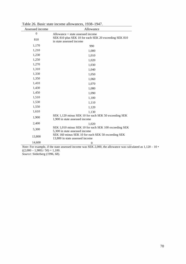
70

Table 26. Basic state income allowances, 1938–1947. Assessed income Allowance

0 Allowance = state assessed income

810 SEK 810 plus SEK 10 for each SEK 20 exceeding SEK 810 in state assessed income

1,170 990 1,210 1,000 1,230 1,010 1,250 1,020 1,270 1,030 1,310 1,040 1,330 1,050 1,350 1,060 1,410 1,070 1,430 1,080 1,450 1,090 1,510 1,100 1,530 1,110 1,550 1,120 1,610 1,130

1,900 SEK 1,120 minus SEK 10 for each SEK 50 exceeding SEK 1,900 in state assessed income

2,400 1,020

5,300 SEK 1,010 minus SEK 10 for each SEK 100 exceeding SEK 5,300 in state assessed income

13,800 SEK 160 minus SEK 10 for each SEK 50 exceeding SEK 13,800 in state assessed income

14,600 0 Note: For example, if the state assessed income was SEK 2,000, the allowance was calculated as 1,120 – 10 • ((2,000 – 1,900) / 50) = 1,100. Source: Söderberg (1996, 68).

71

Table 27. Basic state income allowances, 1948–1952. State assessed income Allowance

State assessed income Allowance

State assessed income Allowance

State assessed income Allowance

0 1,800 4,850 1,340 6,900 880 8,950 420 2,850 1,790 4,900 1,330 6,950 870 9,000 410 2,900 1,780 4,950 1,320 7,000 860 9,030 400 2,950 1,770 5,000 1,310 7,030 850 9,070 390 3,000 1,760 5,030 1,300 7,070 840 9,100 380 3,030 1,750 5,070 1,290 7,100 830 9,150 370 3,070 1,740 5,100 1,280 7,150 820 9,200 360 3,100 1,730 5,150 1,270 7,200 810 9,250 350 3,150 1,720 5,200 1,260 7,250 800 9,300 340 3,200 1,710 5,250 1,250 7,300 790 9,350 330 3,250 1,700 5,300 1,240 7,350 780 9,400 320 3,300 1,690 5,350 1,230 7,400 770 9,430 310 3,350 1,680 5,400 1,220 7,430 760 9,470 300 3,400 1,670 5,430 1,210 7,470 750 9,500 290 3,430 1,660 5,470 1,200 7,500 740 9,550 280 3,470 1,650 5,500 1,190 7,550 730 9,600 270 3,500 1,640 5,550 1,180 7,600 720 9,650 260 3,550 1,630 5,600 1,170 7,650 710 9,700 250 3,600 1,620 5,650 1,160 7,700 700 9,750 240 3,650 1,610 5,700 1,150 7,750 690 9,800 230 3,700 1,600 5,750 1,140 7,800 680 9,830 220 3,750 1,590 5,800 1,130 7,830 670 9,870 210 3,800 1,580 5,830 1,120 7,870 660 9,900 200 3,830 1,570 5,870 1,110 7,900 650 9,950 190 3,870 1,560 5,900 1,100 7,950 640 10,000 180 3,900 1,550 5,950 1,090 8,000 630 10,050 170 3,950 1,540 6,000 1,080 8,050 620 10,100 160 4,000 1,530 6,050 1,070 8,100 610 10,150 150 4,050 1,520 6,100 1,060 8,150 600 10,200 140 4,100 1,510 6,150 1,050 8,200 590 10,230 130 4,150 1,500 6,200 1,040 8,230 580 10,270 120 4,200 1,490 6,230 1,030 8,270 570 10,300 110 4,230 1,480 6,270 1,020 8,300 560 10,350 100 4,270 1,470 6,300 1,010 8,350 550 10,400 90 4,300 1,460 6,350 1,000 8,400 540 10,450 80 4,350 1,450 6,400 990 8,450 530 10,500 70 4,400 1,440 6,450 980 8,500 520 10,550 60 4,450 1,430 6,500 970 8,550 510 10,600 50 4,500 1,420 6,550 960 8,600 500 10,630 40 4,550 1,410 6,600 950 8,630 490 10,670 30 4,600 1,400 6,630 940 8,670 480 10,700 20 4,630 1,390 6,670 930 8,700 470 10,750 10 4,670 1,380 6,700 920 8,750 460 10,800 0 4,700 1,370 6,750 910 8,800 450 4,750 1,360 6,800 900 8,850 440 4,800 1,350 6,850 890 8,900 430

Source: Söderberg (1996, 69–72).

72

Table 28. Basic local and state income tax allowances, 1971–1974. Assessed income Allowance

0 4,500 30,000 4,500 – 0.2 • (T − 30,000) 52,500 0

Note: T = assessed income. Source: Söderberg (1996, 58). Table 29. Basic local and state income tax allowances, 1991–1992.

Note: T = assessed income. The calculated amount is rounded down to closest hundred SEK. Source: Söderberg (1996, 59–60). Table 30. Basic local and state income tax allowances, 1993–1994.

Note: T = assessed income. The calculated amount is rounded down to closest hundred SEK. In 1994, there was no allowance at the state level. Source: Söderberg (1996, 60–61).

Table 31. Basic local and state income tax allowances, 1995–1996.

Note: T = assessed income. The calculated amount is rounded down to closest hundred SEK. Source: Söderberg (1996, 61–62).

Assessed income Allowance Assessed income Allowance 1991 1992 0 10,300 0 10,700

60,300 10,304 + 0.25 • (T − 59,892) 62,800 10,784 + 0.25 • (T − 62,682) 92,700 18,500 97,200 19,400 98,900 18,596 − 0.1 • (T − 97,888) 103,100 19,462 − 0.1 • (T − 102,448) 179,900 10,300 189,100 10,700

Assessed income Allowance Assessed income Allowance 1993 Local 1994 0 11,000 0 8,800

64,400 11,004 + 0.25 • (T − 63,984) 65,900 8,800 + 0.25 • (T − 65,472) 99,200 19,800 101,500 17,800 105,300 19,866 − 0.1 • (T − 104,576) 107,700 17,864 − 0.1 • (T − 107,008) 192,300 11,000 196,700 8,800

Assessed income Allowance Assessed income Allowance 1995 1996 0 8,900 0 8,600

66,700 8,925 + 0.25 • (T − 66,402) 67,400 8,688 + 0.25 • (T − 67,332) 103,200 18,100 104,600 18,000 108,800 18,118 − 0.1 • (T − 108,528) 110,200 18,009 − 0.1 • (T − 110,048) 199,800 8,900 203,200 8,600

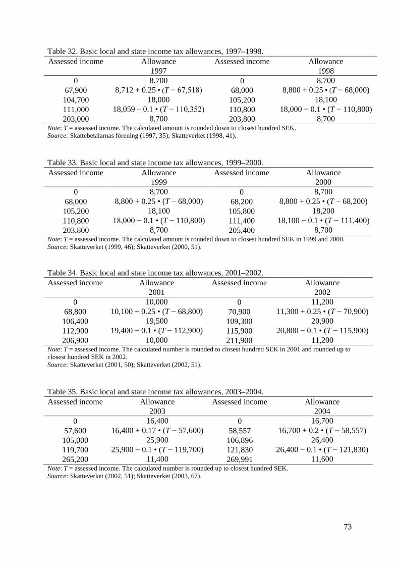
73

Table 32. Basic local and state income tax allowances, 1997–1998.

Note: T = assessed income. The calculated amount is rounded down to closest hundred SEK. Source: Skattebetalarnas förening (1997, 35); Skatteverket (1998, 41).

Table 33. Basic local and state income tax allowances, 1999–2000.

Note: T = assessed income. The calculated amount is rounded down to closest hundred SEK in 1999 and 2000. Source: Skatteverket (1999, 46); Skatteverket (2000, 51).

Table 34. Basic local and state income tax allowances, 2001–2002.

Note: T = assessed income. The calculated number is rounded to closest hundred SEK in 2001 and rounded up to closest hundred SEK in 2002. Source: Skatteverket (2001, 50); Skatteverket (2002, 51).

Table 35. Basic local and state income tax allowances, 2003–2004.

Note: T = assessed income. The calculated number is rounded up to closest hundred SEK. Source: Skatteverket (2002, 51); Skatteverket (2003, 67).

Assessed income Allowance Assessed income Allowance 1997 1998 0 8.700 0 8,700

67,900 8,712 + 0.25 • (T − 67,518) 68,000 8,800 + 0.25 • (T − 68,000) 104,700 18,000 105,200 18,100 111,000 18,059 – 0.1 • (T − 110,352) 110,800 18,000 − 0.1 • (T − 110,800) 203,000 8,700 203,800 8,700

Assessed income Allowance Assessed income Allowance 1999 2000 0 8,700 0 8,700

68,000 8,800 + 0.25 • (T − 68,000) 68,200 8,800 + 0.25 • (T − 68,200) 105,200 18,100 105,800 18,200 110,800 18,000 − 0.1 • (T − 110,800) 111,400 18,100 − 0.1 • (T − 111,400) 203,800 8,700 205,400 8,700

Assessed income Allowance Assessed income Allowance 2001 2002 0 10,000 0 11,200

68,800 10,100 + 0.25 • (T − 68,800) 70,900 11,300 + 0.25 • (T − 70,900) 106,400 19,500 109,300 20,900 112,900 19,400 − 0.1 • (T − 112,900) 115,900 20,800 − 0.1 • (T − 115,900) 206,900 10,000 211,900 11,200

Assessed income Allowance Assessed income Allowance 2003 2004 0 16,400 0 16,700

57,600 16,400 + 0.17 • (T − 57,600) 58,557 16,700 + 0.2 • (T − 58,557) 105,000 25,900 106,896 26,400 119,700 25,900 − 0.1 • (T − 119,700) 121,830 26,400 − 0.1 • (T − 121,830) 265,200 11,400 269,991 11,600

74

Table 36. Basic local and state income tax allowances, 2005. Assessed income Allowance

2005 0 0.423 PBB

1.185 PBB 0.423 + 0.20 • (T − 1.185 PBB) 2.72 PBB 0.73 PBB 3.11 PBB 0.73 PBB − 0.10 • (T − 3.11 PBB) 7.48 PBB 0.293 PBB

Note: PBB = price basic amount (prisbasbelopp). T = assessed income. PBB 2005 = SEK 39,400. The calculated number is rounded up to closest hundred SEK. Source: Skatteverket (2004, 70).

Table 37. Basic local and state income tax allowances, 2006–2013.

Note: PBB = price basic amount (prisbasbelopp). T = assessed income. The calculated number is rounded up to closest hundred SEK. Source: Skatteverket (2005, 68); Skatteverket (2006, 69); Skatteverket (2007, 70); Skatteverket (2008, 70); Skatteverket (2009, 70); Skatteverket (2010, 70); Skatteverket (2011, 70); Skatteverket (2013, 130).

Assessed income Allowance Year PBB 0 0.423 PBB 2006 39,700

0.99 PBB 0.423 PBB + 0.20 • (T − 0.99 PBB) 2007 40,300 2.72 PBB 0.77 PBB 2008 41,000 3.11 PBB 0.77 PBB − 0.10 • (T − 3.11 PBB) 2009 42,800 7.88 PBB 0.293 PBB 2010 42,400

2011 42,800 2012 44,000 2013 44,500

75

Appendix F. National basic pension contribution paid by employees (folkpensionsavgift). Table 38. National basic pension contribution, 1913–1921.

State assessed income Fee

0 3 500 5 800 8

1,200 13 Source: Elmér (1960, 222). Table 39. National basic pension contribution, 1922–1935.

State assessed income Fee

0 3 600 5 800 8

1,200 13 3,000 18 5,000 23 7,000 28 10,000 33

Source: Elmér (1960, 222).

76

Table 40. National basic pension contribution, 1936–1974. Year Fee

1936–1947 1.0 percent of the state assessed income, however at least SEK 6 and at the most SEK 20.

1948–1951 1.0 percent of the state assessed income, however at least SEK 6 and at the most SEK 100.

1952–1953 Same as above although no minimum amount.

1954–1956 1.8 percent of the state assessed income. For unmarried individuals a maximum of SEK 180. No fee if the assessed income is less than SEK 1,200.

1957–1958 2.5 percent of the state assessed income. For unmarried individuals a maximum of SEK 250. No fee if the assessed income is less than SEK 1,200.

1959–1961 4.0 percent of the state assessed income. A maximum of SEK 600 for unmarried individuals. No fee if the assessed income is less than SEK 1,200.

1962–1965 Same as above although the exemption from fee for low incomes is expanded up to SEK 2,400 in state assessed income.

1966 4.0 percent of the state taxable income. A maximum of 1,200 SEK for unmarried individuals.

1967 4.5 percent of the state taxable income. A maximum of 1,350 SEK for unmarried individuals.

1968–1973 5.0 percent of the state taxable income. A maximum of 1,500 SEK per individual.

Source: Söderberg (1996, 111–113).

77

Appendix G. Health insurance fee paid by employees (sjukförsäkringsavgift). Table 41. Health insurance fee, 1955–1962.

Annual wage Fee 1955–1958 1959–1961 1962

0 65 75 100 1,800 75 85 105 2,400 80 90 110 3,000 85 95 115 3,600 95 100 120 4,200 100 105 125 5,000 105 115 135 5,800 110 120 140 6,800 125 130 150 8,400 140 145 165

10,200 155 155 175 12,000 170 170 190 14,000 185 180 200

Note: Because the fee was a fixed amount in SEK within certain income brackets until 1973, the marginal effect within the brackets was zero. Source: Söderberg (1996, 49). Table 42. Health insurance fee, 1963–1966.

Annual wage Fee 1963–1964 1965 1966

0 120 130 140 1,800 120 130 140 2,600 130 135 150 3,400 135 145 155 4,200 140 150 165 5,000 150 160 175 5,800 160 170 185 6,800 170 185 200 8,400 190 200 215

10,200 200 215 235 12,000 215 230 250 14,000 230 245 265 16,000 245 260 285 18,000 265 285 310 21,000 290 310 335

Note: Because the fee was a fixed amount in SEK within certain income brackets until 1973, the marginal effect within the brackets was zero. Source: Söderberg (1996, 50).

78

Table 43. Health insurance fee, 1967–1973. Annual wage Fee

1967 1968 1969 1970 1971 1972 1973 0 145 205 240 240 0 0 0

1,800 145 205 240 240 255 295 310 2,600 155 210 245 245 260 300 320 3,400 160 220 250 255 265 305 325 4,200 165 225 255 260 275 310 335 5,000 170 230 260 265 280 320 340 5,800 185 245 275 280 285 330 355 6,800 195 260 285 295 305 345 370 8,400 205 270 300 305 320 360 385

10,200 225 290 315 325 340 380 405 12,000 245 310 335 345 360 400 425 14,000 260 330 350 365 380 420 450 16,000 280 350 370 385 400 440 470 18,000 295 370 390 405 420 460 490 21,000 315 390 405 425 440 475 515 24,000 335 410 425 445 460 495 535 27,000 350 430 440 465 480 515 555 30,000 370 450 460 485 500 535 575 33,000 385 470 485 505 520 555 600 36,000 405 490 495 525 540 575 620 39,000 425 510 515 545 560 595 640

Note: Because the fee was a fixed amount in SEK within certain income brackets until 1973, the marginal effect within the brackets was zero. Source: Söderberg (1996, 51). Table 44. Health insurance fee, 1974.

1974 SEK 300 + 1.6 percent of salary up to SEK 60,750. (Hence, the maximum fee was SEK 1,272.)

Source: Söderberg (1996, 52).

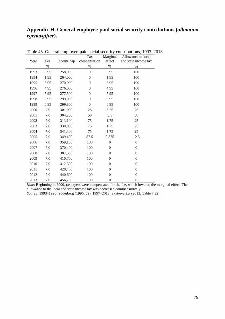
79

Appendix H. General employee-paid social security contributions (allmänna egenavgifter). Table 45. General employee-paid social security contributions, 1993–2013.

Year Fee Income cap Tax

compensation Marginal

effect Allowance to local

and state income tax % % % %

1993 0.95 258,000 0 0.95 100 1994 1.95 264,000 0 1.95 100 1995 3.95 270,000 0 3.95 100 1996 4.95 276,000 0 4.95 100 1997 5.95 277,500 0 5.95 100 1998 6.95 299,000 0 6.95 100 1999 6.95 299,800 0 6.95 100 2000 7.0 301,000 25 5.25 75 2001 7.0 304,200 50 3.5 50 2002 7.0 313,100 75 1.75 25 2003 7.0 330,000 75 1.75 25 2004 7.0 341,300 75 1.75 25 2005 7.0 349,400 87.5 0.875 12.5 2006 7.0 359,100 100 0 0 2007 7.0 370,400 100 0 0 2008 7.0 387,300 100 0 0 2009 7.0 410,700 100 0 0 2010 7.0 412,300 100 0 0 2011 7.0 420,400 100 0 0 2012 7.0 440,600 100 0 0 2013 7.0 456,700 100 0 0

Note: Beginning in 2000, taxpayers were compensated for the fee, which lowered the marginal effect. The allowance to the local and state income tax was decreased commensurately. Source: 1993–1996: Söderberg (1996, 52). 1997–2013: Skatteverket (2013, Table 7.32).

80

Appendix I. Income tax credits (skattereduktion för arbetsinkomster). Table 46. Tax credits, 1999–2002.

Income Tax credit 0 1,320

135,000 SEK 1,320 minus 1.2% times the income exceeding SEK 135,000

245,000 0 Note: 1999–2001: Income refers to pension-entitled income. In 2002, it refers to taxable income. Source: Skatteverket (2002, 50). Table 47. Earned income tax credit, 2007. Income from active

work per year (AI)

Tax credit

0 (AI − GA) • KI

0.79 PBB (0.79 PBB + 0.2 • (AI − 0.79 PBB) − GA) • KI

2.72 PBB (1.176 PBB − GA) • KI Note: Refers to persons below age 65. PBB = Price basic amount according to the National Insurance Act AI = Labor income GA = The sum of all basic allowances and sea income tax reduction KI = The tax rate for municipal income tax In 2007, the price basic amount was SEK 40,300. Source: Ministry of Finance (2006, 46–47).

Table 48. Earned income tax credit, 2008. Income from active

work per year (AI)

Tax credit

0 (AI − GA) • KI

0.91 PBB (0.91 PBB + 0.2 • (AI − 0.91 PBB) − GA) • KI

2.72 PBB (1.272 PBB + 0.033 • (AI − 72 PBB) − GA) • KI

7.00 PBB (1.413 PBB − GA) • KI Note: Refers to persons below age 65. PBB = Price basic amount according to the National Insurance Act AI = Labor income GA = The sum of all basic allowances and sea income tax reduction KI = The tax rate for municipal income tax In 2008, the price basic amount was SEK 41,000. Source: Ministry of Finance (2007, 43).

81

Table 49. Earned income tax credit, 2009. Income from active

work per year (AI)

Tax credit

0 (AI − GA) • KI 0.91 PBB (0.91 PBB + 0.25 • (AI − 0.91 PBB) − GA) • KI

2.72 PBB (1.363 PBB + 0.065 • (AI − 2.72 PBB) − GA) • KI

7.00 PBB (1.642 PBB − GA) • KI Note: Refers to persons below age 65. PBB = Price basic amount according to the National Insurance Act AI = Labor income GA = The sum of all basic allowances and sea income tax reduction KI = The tax rate for municipal income tax In 2009, the price basic amount was SEK 42,800. Source: Ministry of Finance (2008, 46–47).

Table 50. Earned income tax credit, 2010–2013 Income from active

work per year (AI)

Tax credit

0 (AI − GA) • KI 0.91 PBB (0.91 PBB + 0.304 • (AI − 0.91 PBB) − GA) • KI

2.72 PBB (1.461 PBB + 0.095 • (AI − 2.72 PBB) − GA) • KI

7.00 PBB (1.868 PBB − GA) • KI Note: Refers to persons below age 65. PBB = Price basic amount according to the National Insurance Act AI = Labor income GA = The sum of all basic allowances and sea income tax reduction KI = The tax rate for municipal income tax In 2010 (2011; 2012; 2013) the price basic amount was SEK 42,400 (42,800; 44,000; 44,500). Source: Ministry of Finance (2009, 61–62); Ministry of Finance (2010, 66); Ministry of Finance (2011, 66); Ministry of Finance (2012, 68).

82

Appendix J. Employer-paid social security contributions (arbetsgivaravgifter).

Table 51. Employer-paid social security contributions, 1955–2013. Year Fee, % Levied on 1955–1959 1.14 wage share up to SEK 15,000 1960 1.14 wage share up to SEK 4,200 4.14 wage share between SEK 4,200 and SEK 15,000 3,00 wage share between SEK 15,000 and SEK 31,500 1961 1.14 wage share up to SEK 4,300 5.14 wage share between SEK 4,300 and SEK 15,000 4.00 wage share between SEK 15,000 and SEK 32,250 1962 1.14 wage share up to SEK 4,500 6.14 wage share between SEK 4,500 and SEK 15,000 5,00 wage share between SEK 15,000 and SEK 33,750 1963 1.50 wage share up to SEK 4,700 7.50 wage share between SEK 4,700 and SEK 22,000 6,00 wage share between SEK 22,000 and SEK 35,250 1964 1.50 wage share up to SEK 4,800 8.50 wage share between SEK 4,800 and SEK 22,000 7.00 wage share between SEK 22,000 and SEK 36,000 1965 1.50 wage share up to SEK 5,000 9.00 wage share between SEK 5,000 and SEK 22,000 7.50 wage share between SEK 22,000 and SEK 37,500 1966 1.50 wage share up to SEK 5,300 9.50 wage share between SEK 5,300 and SEK 22,000 8.00 wage share between SEK 22,000 and SEK 39,750 1967 2.60 wage share up to SEK 5,500 11.1 wage share between SEK 5,500 and SEK 41,250 1968 2.60 wage share up to SEK 5,700 11.6 wage share between SEK 5,700 and SEK 42,750 1969 3.60 wage share up to SEK 5,800 13.1 wage share between SEK 5,800 and SEK 43,500 1.00 wage share exceeding SEK 43,500 1970 3.90 wage share up to SEK 6,000 13.9 wage share between SEK 6,000 and SEK 45,000 1.00 wage share exceeding SEK 45,000 1971 5.12 wage share up to SEK 6,400 15.37 wage share between SEK 6,400 and SEK 48,000 2.00 wage share exceeding SEK 48,000 1972 5.47 wage share up to SEK 7,100 15.97 wage share between SEK 7,100 and SEK 53,250 2.00 wage share exceeding SEK 53,250 1973 7.57 wage share up to SEK 7,300 18.07 wage share between SEK 7,300 and SEK 54,750

83

Year Fee, % Levied on 4.00 wage share exceeding SEK 54,750 1974 11.87 wage share up to SEK 8,100 22.37 wage share between SEK 8,100 and SEK 60,750 4.00 wage share exceeding SEK 60,750 1975 15.97 wage share up to SEK 9,000 26.72 wage share between SEK 9,000 and SEK 67,500 4.00 wage share exceeding SEK 67,500 1976 19.675 wage share up to SEK 9,700 30.675 wage share between SEK 9,700 and SEK 72,750 19.675 wage share exceeding SEK 72,750 1977 22.95 wage share up to SEK 10,700 34.7 wage share between SEK 10,700 and SEK 80,250 22.95 wage share exceeding SEK 80,250 1978 21.97 wage share up to SEK 11,800 33.72 wage share between SEK 11,800 and SEK 88,500 21.97 wage share exceeding SEK 88,500 1979 22.38 wage share up to SEK 13,100 34.13 wage share between SEK 13,100 and SEK 98,250 22.38 wage share exceeding SEK 98,250 1980 23.25 wage share up to SEK 13,900 35.25 wage share between SEK 13,900 and SEK 104,250 23.25 wage share exceeding SEK 104,250 1981 23.605 wage share up to SEK 16,100 35.855 wage share between SEK 16,100 and SEK 120,750 23.605 wage share exceeding SEK 120,750 1982 33.055 full wage 1983 36.255 full wage 1984 36.155 full wage 1985 36.455 full wage 1986 36.45 full wage 1987 37.076 full wage 1988 37.07 full wage 1989 37.97 full wage 1990 38.97 full wage 1991 38.03 full wage 1992 34.83 full wage 1993 31.00 full wage 1994 31.36 full wage 1995 32.86 full wage 1996 33.06 full wage 1997 32.92 full wage 1998 33.03 full wage 1999 33.06 full wage 2000 32.92 full wage 2001 32.82 full wage

84

Year Fee, % Levied on 2002 32.82 full wage 2003 32.82 full wage 2004 32.70 full wage 2005 32.46 full wage 2006 32.28 full wage 2007 32.42 full wage 2008 32.42 full wage 2009 31.42 full wage 2010 31.42 full wage 2011 31.42 full wage 2012 31.42 full wage 2013 31.42 full wage Note: Including the unspecified payroll tax (allmän arbetsgivaravgift). Source: 1955–1996: Söderberg (1996, 117–119); 1997–2013: Skatteverket (2013, Table 7.32).

85

References

Agell, Jonas, Peter Englund, and Jan Södersten. 1995. “Svensk skattepolitik i teori och

praktik. 1991 års skattereform.” In Ekonomiska Rådets rapport till kommittén för

utvärdering av skattereformen, bilaga 1, SOU 1995:104. Stockholm: Fritzes.

Agell, Jonas, Peter Englund, and Jan Södersten. 1998. Incentives and Redistribution in the

Welfare State: The Swedish Tax Reform. London: Macmillan.

Aidt, Toke S. and Peter S. Jensen. 2009. “Tax Structure, Size of Government, and the

Extension of the Voting Franchise in Western Europe, 1860–1938.” International Tax

and Public Finance 16(3), 362–394.

Barro, Robert J. and Chaipat Sahasakul. 1986. “Average Marginal Tax Rates from Social

Security and the Individual Income Tax.” Journal of Business 59(4), 555–566.

Bassanini, Andrea and Duval Romain. 2006. “Employment Patterns in OECD Countries:

Reassessing the Role of Policies and Institutions.” OECD Economics Department

Working Paper 486. Paris: OECD.

Bentzel, Ragnar. 1952. Inkomstfördelningen i Sverige. Stockholm: Industriens

Utredningsinstitut.

Bergh, Andreas. 2014. “What Are the Policy Lessons from Sweden? On the Rise, Fall and

Revival of a Capitalist Welfare State.” New Political Economy 19(5), 662–694.

Birkinshaw Julian, Pontus Braunerhjelm, Ulv Holm, and Siri A. Terjeseni. 2006. “Why Do

Some Corporations Relocate their Headquarters Overseas?” Strategic Management

Journal 27(7), 681–700.

Braunerhjelm, Pontus. 2004. “Heading for Headquarters? Why and How the Location of

Headquarters Matter among the EU-Countries.” In European Union and the Race for

Foreign Direct Investment in Europe, edited by Lars Oxelheim and Pervez N. Ghauri,

123–148. Amsterdam and Boston: Elsevier.

Confederation of Swedish Enterprise. 2014. Fakta om löner och arbetstider 2014. Stockholm:

Svenskt Näringsliv.

Corneo, Giacomo. 2005. “The Rise and Likely Fall of the German Income Tax, 1958–2005.”

CESifo Economic Studies 51(1), 159–186.

Dahlgren, Stellan and Kekke Stadin, eds. 1990. Från feodalism till kapitalism: skatternas roll

i det svenska samhällets omvandling 1720–1910. Uppsala: Department of History,

Uppsala University.

86

Daveri, Francesco and Guido Tabellini. 2000. “Unemployment, Growth and Taxation in

Industrial Countries.” Economic Policy 15(30), 49–104.

de Haan, Jacob, Jan-Egbert Sturm, and Björn Volkerink. 2004. “How to Measure the Tax

Burden on Labor at the Macro Level?” In Measuring the Tax Burden on Capital and

Labor, edited by Peter Birch Sørensen, 289–318. Cambridge, MA: MIT Press.

Disney, Richard. 2006. “Household Saving Rates and the Design of Public Pension

Programmes: Cross-Country Evidence.” National Institute Economic Review 198(1), 61–

74.

Disney, Richard, Tito Boeri, and Tullio Jappelli. 2004. “Are Contributions to Public Pension

Programmes a Tax on Employment?” Economic Policy 19(39), 267–311.

Du Rietz, Gunnar. 1994. Välfärdsstatens finansiering. Stockholm: City University Press.

Du Rietz, Gunnas and Magnus Henrekson. 2015. ”Swedish Wealth Taxation (1911–2007).”

IFN Working Paper nr 1000, published as chapter 6, pp.267–302 in Swedish Taxation:

Developments since 1862, edited by Magnus Henrekson and Mikael Stenkula, 267–302.

New York: Palgrave Macmillan.

Eberstein, Gösta. 1929. Om skatt till stat och kommun enligt svensk rätt: Förra delen.

Stockholm: Norstedts.

Eberstein, Gösta. 1937. Om skatt till stat och kommun enligt svensk rätt: Senare delen.

Stockholm: Norstedts.

Edvinsson, Rodney. 2005. “Growth, Accumulation, Crises: With New Macroeconomic Data

for Sweden.” PhD diss., Stockholm University.

Elmér, Åke. 1960. ”Folkpensioneringen i Sverige med särskild hänsyn till

ålderspensioneringen.” PhD diss., Lund University.

Elvander, Nils. 1972. Svensk skattepolitik 1945–1970: En studie i partiers och

organisationers funktioner. Stockholm: Rabén & Sjögren.

Esping-Andersen, Gösta. 1990. The Three Worlds of Welfare Capitalism. Princeton, NJ:

Princeton University Press.

Ekonomistyrningsverket. 2010. Tidsserier, Statsbudgeten m.m. 2009. ESV 2010:20.

Stockholm: Ekonomistyrningsverket [Swedish National Financial Management

Authority].

Ekonomistyrningsverket. 2011. Tidsserier, Statsbudgeten m.m. 2010. ESV 2011:21.

Stockholm: Ekonomistyrningsverket [Swedish National Financial Management

Authority].

87

Ekonomistyrningsverket. 2012. Tidsserier, Statsbudgeten m.m. 2011. ESV 2012:28.

Stockholm: Ekonomistyrningsverket [Swedish National Financial Management

Authority].

Ekonomistyrningsverket. 2013. Tidsserier, Statsbudgeten m.m. 2012. ESV 2013:38.

Stockholm: Ekonomistyrningsverket [Swedish National Financial Management

Authority].

Ekonomistyrningsverket. 2014. Tidsserier, Statsbudgeten m.m. 2013. ESV 2014:41.

Stockholm: Ekonomistyrningsverket [Swedish National Financial Management Authority].

Feldt, Kjell-Olof. 1991. Alla dessa dagar: i regeringen 1982–1990. Stockholm: Norstedts.

Gårestad, Peter. 1987. ”Industrialisering och beskattning i Sverige 1861–1914.” PhD diss.,

Uppsala University.

Genberg, Torsten. 1942. Skatteutvecklingen sedan sekelskiftet. Stockholm: Skattebetalarnas

förening [Swedish Taxpayers’ Association].

Gustafsson, Siv. 1992. “Separate Taxation and Married Women’s Labor Supply. A

Comparison of West Germany and Sweden.” Journal of Population Economics 5(1), 61–

85.

Hansson, Åsa. 2000. “Limits of Tax Policy.” PhD diss., Lund University.

Heady, Christopher. 2004. “The ‘Taxing Wages’ Approach to Measuring the Tax Burden on

Labor.” In Measuring the Tax Burden on Capital and Labor, edited by Peter Birch

Sørensen, 263–287. Cambridge, MA: MIT Press.

Hedlund-Nyström, Torun. 1972. “The Finance Act of 1862 and its Effect on the Economy.”

Economy and History 15(1), 58–82.

Henrekson, Magnus. 1993. “The Peacock-Wiseman Hypothesis.” In The Growth of the Public

Sector, Theories and International Evidence, edited by Norman Gemmell, 53–71.

Cheltenham, UK and Northampton, MA: Edward Elgar Publishing.

Henrekson, Magnus. 1996. “Sweden’s Relative Economic Performance: Lagging Behind or

Staying on Top?” Economic Journal 106(439), 1747–1759.

Henrekson, Magnus and Nathan Rosenberg. 2001. ”Designing Efficient Institutions for

Science-Based Entrepreneurship: Lessons from the US and Sweden.” Journal of

Technology Transfer 26(3), 207–231.

Higgs, Robert. 1987. Crisis and Leviathan: Critical Episodes in the Growth of American

Government. New York: Oxford University Press.

88

Immervoll, Herwig. 2004. “Average and Marginal Effective Tax Rates Facing Workers in the

EU: A Micro-Level Analysis of Levels, Distributions and Driving Factors.” OECD

Social, Employment and Migration Working Paper No. 19. Paris: OECD.

Jaimovich, Nir and Sergio Rebelo. 2012. “Non-Linear Effects of Taxation on Growth.”

NBER Working Paper No. 18473. Cambridge, MA: National Bureau of Economic

Research.

Jakobsson, Ulf and Göran Normann. 1972. Inkomstbeskattningen i den ekonomiska politiken.

Stockholm: Industriens Utredningsinstitut and Almqvist & Wiksell.

Johansson, Dan. 2004. “Skatternas utveckling, omfattning och fördelning.” In Skatter och

värdighet, edited by Dan Johansson, Nils Karlson, and Richard Johnsson, 66–94.

Stockholm: Ratio.

Jungenfelt, Karl G. 1966. Löneandelen och den ekonomiska utvecklingen. Stockholm:

Industriens Utredningsinstitut and Almqvist & Wiksell.

Lewin, Bengt. 2009. Efter skattereformen. En genomgång av svensk skattepolitik 1992–2009.

Stockholm: Riksrevisionen.

Lindbeck, Assar. 1997. ”The Swedish Experiment.” Journal of Economic Literature 35(3) ,

1273–1319.

Lindbeck, Assar. 2012. Ekonomi är att välja. Stockholm: Albert Bonniers Förlag.

Lodin, Sven-Olof. 2011. The Making of Tax Law. Uppsala and Amsterdam: Justus Förlag and

International Bureau of Fiscal Documentation (IBFD).

Löwnertz, Susanne. 2003. De svenska skatternas historia. Stockholm: Riksskatteverket.

Madrick, Jeff. 2009. The Case for Big Government. Princeton, NJ: Princeton University Press.

McKee, Michael, Jacob Visser, and Peter Saunders. 1986. “Marginal Tax Rates on the Use of

Labor and Capital in OECD Countries.” OECD Economic Studies 7, 45–101.

Ministry of Finance. 2006–2012. Beräkningskonventioner. Stockholm: Finansdepartementet.

OECD. 2006. “Special Feature: Broadening the Definition of the Average Worker.” In Taxing

Wages 2004. Paris: OECD.

OECD. 2009. “Special Feature: Consumption Taxation as an Additional Burden on Labor

Income.” In Taxing Wages 2008. Paris: OECD.

OECD. 2010. Taxing Wages 2008–2009. Paris: OECD.

OECD. 2011. Taxing Wages 2010. Paris: OECD.

Orhnial, A. J. H. and Lucien Foldes. 1975. “Estimates of Marginal Tax Rates for Dividends

and Bond Interest in the United Kingdom 1919–1970.” Economica 42(165), 79–91.

89

Peacock, Alan T. and Jack Wiseman. 1961. The Growth of Public Expenditure in the United

Kingdom. Princeton, NJ: Princeton University Press.

Poterba, James M.. 2004. “Taxation and Corporate Payout Policy.” American Economic

Review 94(2), 171–175.

Prado, Svante. 2010. “Nominal and Real Wages of Manufacturing Workers, 1860–2007.” In

Historical Monetary and Financial Statistics for Sweden, Vol. 1, Exchange Rates, Prices

and Wages, 1277–2008, edited by Rodney Edvinsson, Tor Jacobson, and Daniel

Waldenström, 479–572. Stockholm: Ekerlids Förlag.

Rodriguez, Enrique. 1980. Offentlig inkomstexpansion: en analys av drivkrafterna bakom de

offentliga inkomsternas utveckling i Sverige under 1900-talet. Lund: Liber Läromedel.

Rodriguez, Enrique. 1981. Den svenska skattehistorien. Lund: Liber Läromedel.

Roine, Jesper, Jonas Vlachos, and Daniel Waldenström. 2009. “The Long-Run Determinants

of Inequality: What Can we Learn from Top Income Data?” Journal of Public Economics

93(7–8), 974–988.

Roine, Jesper and Daniel Waldenström. 2008. “The Evolution of Top Incomes in an

Egalitarian Society: Sweden, 1903–2004.” Journal of Public Economics 92(1–2), 366–

387.

Rydqvist, Kristian, Joshua D. Spizman, and Ilya A. Strebulaev. 2014. “Government Policy

and Ownership of Equity Securities.” Journal of Financial Economics 111(1), 70–85.

Saez, Emmanuel. 2004. “Reported Incomes and Marginal Tax Rates, 1960–2000: Evidence

and Policy Implications.” In Tax Policy and the Economy, edited by James M. Poterba,

113–173. Cambridge, MA: MIT Press.

SFS 1861:34. Bewillningsförordning 1862.

SFS 1871:30. Kongl. Maj:ts nådiga förordning, angående utgörande af en särskild

tilläggsbewillning för år 1893.

SFS 1879:25. Kongl. Maj:ts nådiga kungörelse, angående särskild tilläggsbevillning för år

1879 och 1880.

SFS 1880:46. Kongl. Maj:ts nådiga kungörelse, angående särskild tilläggsbevillning för år

1881.

SFS 1881:29. Kongl. Maj:ts nådiga kungörelse, angående särskild tilläggsbevillning för år

1882.

SFS 1883:51. Kongl. Maj:ts nådiga förordning angående bevillning af fast egendom samt af

inkomst.

90

SFS 1892:44. Kongl. Maj:ts nådiga förordning angående bevillning af fast egendom samt af

inkomst.

SFS 1892:111. Kongl. Maj:ts nådiga förordning, angående särskild tilläggsbevillning för år

1893.

SFS 1893:34. Kongl Maj:ts nådiga förordning, angående särskild tilläggsbevillning för år

1894.

SFS 1894:76. Kongl. Maj:ts nådiga kungörelse angående den vid 1894 års riksdag åtagna

bevillning af fast egendom samt af inkomst.

SFS 1895:62. Kongl. Maj:ts nådiga kungörelse angående den vid 1895 års riksdag åtagna

bevillning af fast egendom samt af inkomst och angående särskild tilläggsbevillning för

år 1896.

SFS 1897:111. Kongl. Maj:ts nådiga förordning angående bevillning af fast egendom samt af

inkomst.

SFS 1901:31. Kongl. Maj:ts nådiga kungörelse angående den vid 1901 års riksdag åtagna

bevillning af fast egendom samt af inkomst.

SFS 1901:34. Kongl. Maj:ts nådiga förordning angående särskild tilläggsbevillning för år

1901.

SFS 1902:50. Kongl. Maj:ts nådiga kungörelse angående den vid 1902 års riksdag åtagna

bevillning af fast egendom samt af inkomst.

SFS 1902:84. Kongl. Maj:ts nådiga förordning om inkomstsskatt.

SFS 1910:115. Kongl. Maj:ts nådiga förordning om inkomst- och förmögenhetsskatt.

SFS 1910:116. Kongl. Maj:ts nådiga förordning angående bevillning af fast egendom samt af

inkomst.

SFS 1917:513. Fastställelse av vissa till ledning vid uträknandet av extra inkomst- och

förmögenhetsskatt för år 1918 erforderliga tabeller.

SFS 1918:512. Tilläggsskatt för år 1918 års inkomst och förmögenhet.

SFS 1918:513. Extra inkomst- och förmögenhetsskatt för år 1919.

SFS 1920:759. Kungl. Maj:ts förordning om ändring i vissa delar av förordningen den 28

oktober 1910 (n:r 116) angående bevillning av fast egendom samt av inkomst.

Skattebetalarnas förening. 1997. Fakta för skattebetalare. Stockholm: Skattebetalarnas

förening [Swedish Taxpayers’ Association].

Skatteverket. 1998–2013. Tax Statistical Yearbook of Sweden 1998–2013. Stockholm:

Skatteverket [Swedish Tax Agency].

91

Söderberg, Hans. 1996. Inkomstskattens utveckling under 1900-talet. En vägvisare för

skatteberäkningar åren 1921–1996. Stockholm: Skattebetalarnas förening [Swedish

Taxpayers’ Association].

Sørensen, Peter Birch, ed. 2004. Measuring the Tax Burden on Capital and Labor.

Cambridge, MA: MIT Press.

SOU 1989:33. Reformerad inkomstbeskattning, del 1, skattereformens huvudlinjer.

Stockholm: Fritzes.

Statistics Sweden. 1914–2011. Statistical Yearbook of Sweden. Stockholm: Statistics Sweden.

Stenkula, Mikael. 2015. “Taxation of Goods and Services in Sweden (1862–2013).” IFN

Working Paper nr 956, published as chapter 4, pp. 179–221 in Swedish Taxation:

Developments since 1862, edited by Magnus Henrekson and Mikael Stenkula. New York:

Palgrave Macmillan.