SWIMMING, PUMPING AND GLIDING AT LOWREYNOLDS NUMBER

Research Thesis

Submitted in partial fulfillment of the requirements for the degree of

Master of Science in Physics

Oren Raz

Submitted to the Senate of the Technion - Israel Institute of Technology

Hodesh 5768 HAIFA December 2007

This research thesis was done under the supervision of Associate

Prof. Joseph Avron in the Faculty of Physics, and Prof.

Alexander Leshansky in the Faculty of Chemical Engineering.

I would like to thank Dr. Oded kenneth for his contributions.

I would like to thank my wife Michal for her support.

The generous financial support of

The Technion

is gratefully acknowledged.

Contents

Abstract 1

List of Symbols 2

1 Introduction 5

1.1 Motivation . . . . . . . . . . . . . . . . . . . . . . . . . . . . . . . . . . . . 5

1.2 Low Reynolds numbers hydrodynamics - Stokes equation . . . . . . . . . . 5

1.3 Lorenz Reciprocity . . . . . . . . . . . . . . . . . . . . . . . . . . . . . . . 6

2 Purcell’s three linked swimmer, and it’s symmetrizations 9

2.1 Introduction . . . . . . . . . . . . . . . . . . . . . . . . . . . . . . . . . . . 9

2.2 Purcell’s three linked swimmer . . . . . . . . . . . . . . . . . . . . . . . . . 9

2.3 The symmetric purcell’s swimmer . . . . . . . . . . . . . . . . . . . . . . . 13

2.4 The most efficient stroke . . . . . . . . . . . . . . . . . . . . . . . . . . . . 16

2.5 Swimming in different viscosities . . . . . . . . . . . . . . . . . . . . . . . . 17

3 Swimming, Pumping and Gliding at low Reynolds number 21

3.1 Introduction . . . . . . . . . . . . . . . . . . . . . . . . . . . . . . . . . . . 21

3.2 Anchoring as a choice of gauge . . . . . . . . . . . . . . . . . . . . . . . . . 22

3.3 Triality of swimmer pumps and gliders . . . . . . . . . . . . . . . . . . . . 23

3.4 Linear swimmers and optimal anchoring . . . . . . . . . . . . . . . . . . . 25

3.5 Helices as swimmers and pumps . . . . . . . . . . . . . . . . . . . . . . . . 27

3.6 Pumps that do not swim . . . . . . . . . . . . . . . . . . . . . . . . . . . . 28

4 Summary 31

A The three linked swimmer as a pump 33

i

List of Figures

1 Purcell’s three linked rods . . . . . . . . . . . . . . . . . . . . . . . . . . . 9

2 Fφ(θ1, θ2) for Purcell’s three linked swimmer (in radians) . . . . . . . . . . 13

3 Upper: Fy(θ1, θ2), Lower: Fx(θ1, θ2) for the Purcell’s three linked swimmer

(in l1 units) . . . . . . . . . . . . . . . . . . . . . . . . . . . . . . . . . . . 14

4 The symmetrized purcell’s swimmer . . . . . . . . . . . . . . . . . . . . . . 15

5 The optimal stroke for the symmetric purcell swimmer, plotted on F (θ1, θ2)

for this swimmer . . . . . . . . . . . . . . . . . . . . . . . . . . . . . . . . 18

6 5-Links, A swimmer which changes its moving direction when putted in

more viscous fluid . . . . . . . . . . . . . . . . . . . . . . . . . . . . . . . . 19

7 F (θ1, θ2) for the 5-Links swimmer . . . . . . . . . . . . . . . . . . . . . . . 20

8 A treadmiller transports its skin from head to back. The treadmiller in the

figure swims to the left while the motion of its skin guarantees that,in the

limit of large aspect ratio, the ambient fluid is left almost undisturbed. If

it is anchored at the gray point then it transfers momentum to the fluid (to

the right). The power of towing a frozen treadmiller and of pumping almost

coincide reflecting the fact that a treadmiller swims with little dissipation. 26

9 A Purcell three linked swimmer, left, controls the two angles θ1 and θ2.

When bolted it effectively splits into two independent wind-shield wipers

each of which is self retracing. It will, therefore, not pump. Pushmepullyou,

right, controls the distance between the two spheres and the ratio of their

volumes. It can have arbitrarily large swimming efficiency. . . . . . . . . . 29

ii

iii

iv

Abstract

This research is about micro-swimmers, micro-pumps and the relations between them.

First, I study what swimming at low Reynolds number is, through few simple examples:

the first one is the famous Purcell’s three linked swimmer, made of three slender rods,

which can control the angles between the rods. This example demonstrate the non-

trivial behavior of even a very simple swimmer at low Reynolds number, and I use the

Wilczek-Shapere formalism [30] to give a partial analysis for this swimmer (problems like

optimal strokes are not considered). Since this swimmer is very complicated to analyzed,

I introduce some modifications (symmetrization) on this swimmer, which makes it much

simpler to analyzed. On this modified Pursell’s swimmer I can carry on many calculations

which are too complicated for the Purcell’s three linked swimmer, like fastest stroke or

most efficient stroke. I also introduce other modification that can explain how, in some

cases, swimming can be better in more viscose fluid.

After understanding, through the examples, what swimming at low Reynolds is, I

connect swimming to pumping an gliding, through the linearity of Stokes equation and

the Lorenz reciprocity. It turns out that the relations between a swimmer, a glider and

the pump one gets by anchoring the swimmer are simple, and can shed light on both

swimmer and pumps property. I also solve some optimization problems, like what will be

the optimal pitch for a helix as a pump ad as a swimmer and where to anchor a linear

swimmer in order to get the best pump. I end up by giving examples for a swimmer that

will not pump and a pump that will not swim.

1

List of Symbols

symbol Meaning

v velocity field

f external force (per mass unit)

p pressure

p modified pressure

ρ mass density

µ dynamic viscosity

Φ external potential

U characteristic velocity

L characteristic length

Re Reynolds number

Σ fluid volume

γ a stroke

V linear velocity

ω angular velocity

V (V, ω) - 6 dimensional vector

πij stress tensor

F force

N torque

F (F, N) - 6 dimensional vector

r position

dSj surface element

θi, φ angles in swimmers

x, y position of a point in a swimmer

2

symbol Meaning

li arm length in a swimmer

η arms ratio in Purcell’s swimmer

t tangent unit vector

κ aspect ratio of a slender body

A;A; A gauge field

F ;F ; F strength field

R rotation matrix

S(γ) surface bounded by γ

ε small parameter

∆X change in swimmers place after full stroke

E energy dissipation in full stroke

ga,b the dissipation metric on shape space

P Power

ε swimmers efficiency

τ stroke time

q Lagrange multiplier

Sq action

M grand resistance matrix

K resistance matrix (between F and V)

C coupling matrix (between F and ω)

Ω rotation resistance matrix (between N and ω)

R antisymmetric matrix associated with r

Hij Oseen tesor

a sphere radius

q arm length

∆q amplitude of changes in arm length

3

4

1 Introduction

1.1 Motivation

The last few decades showed a growing interest in swimming at the micro and nano

scales, motivated by both biological and engineering problems: in biology, questions about

microorganisms locomotion inspired research on flagellar propulsions [13, 20, 29] and

some other propulsion techniques as well [11, 27, 15], while the engineering effort to build

artificial micro-swimmers [25, 16, 21] has led to questions about other aspects of swimming

at low Reynolds.

The following work has two parts: the first one is about some specific problems in

swimming at low Reynolds number (the Purcell’s three linked swimmer and some mod-

ifications of this swimmer), and the second one is about general correlations between

swimmers, pumps and dragged bodies (gliders) at low Reynolds number. Both of these

problems were inspired by experimental questions: the Purcell’s three linked swimmer is

a first order approximation for a swimmer built by Gabor Kosa and Moshe Shoham [16]

in the Mechanical Engineering faculty at the Technion, and the swimmer-pump relations

where motivated by both the need of microscopic pumps [14] for ”Lab on a Chip devices”

and the experimental comfort of measuring bolted swimmers rather than free ones [4, 32].

1.2 Low Reynolds numbers hydrodynamics - Stokes equation

As has been stressed nicely in Purcell’s canonical paper ”Life at Low Reynolds number”

[23], motion at the micro scale is different from our everyday experiences. Here I shall give

a short derivation for the stokes equation which governs the motion of micro swimmers,

pumps and gliders.

The fundamental equations governing motion of bodies in an incompressible fluid are

Naviar-Stokes equations (together with the incompressibility equation) [17]:

ρ

(∂v

∂t+ (v · ∇)v

)= ρf −∇p + µ4v ; ∇ · v = 0 (1.1)

where v is the velocity field, ρ is the mass density, f is external force per mass unit (eg.

gravity), p is the pressure field and µ is the viscosity of the fluid. In the cases of constant

ρ and when f is caused by some potential (that is f = −∇Φ for some potential Φ), we can

use the modified pressure to unified the pressure and volume force in Eq. (1.1): p = p+ρΦ,

5

and ∇p = ∇p− ρf . Under these assumptions Eq. (1.1) becomes

−ρ

((v · ∇)v +

∂v

∂t

)+ µ4v = ∇p

The firs term in the left hand side of this equation is called the inertia term, and the

second one is called the viscosity term. If the characteristic length of the problem at hand

is L, the characteristic velocity is U and the time scale for the changes in v is comparable

with LU, we can approximate the order of the Inertia and viscosity terms as: ρU2

Land µU

L2 ,

respectively. The ratio between the inertial and the viscosity terms is called the Reynolds

number, and is given by:

Re =ρUL

µ

In cases Re ¿ 1, the inertial term can be neglected from the equation, and the remain

equations will be

∇p = µ4v ; ∇ · v = 0 (1.2)

The first one is known as Stokes equation, and the second one is the incompressibility

equation. The physical characters of systems with a very low Reynolds number is that in-

ertia is completely negligible: the movement of a body depends only on the instantaneous

forces acting on it, and not on the velocity it had in the past – there is no ”memory”

in the system. This also means that at low Reynolds number a body is consider to be

in a constant (angular) velocity, although the constant might changes with time: the

acceleration time is negligible, so that at any moment the (angular) velocity is considered

as a constant, with zero (angular) acceleration. This implies that the sum of all forces

(torques) on a body is always zero. In the case of dragged/anchored body, the total force

(torque) the fluid applies on a body is equal in magnitude but opposite in sign to the

dragging/anchoring force (torque). In the case of a free body (like a swimmer), where all

the forces (toques) are inner ones and thus summed to zero, the friction forces (torques)

applied by the fluid on the body must also summed to be zero.

1.3 Lorenz Reciprocity

The exact solutions to Eq. (1.2) in three dimensions are known for only small number of

geometries [12]: ellipsoids. Good approximations are known only for cases of many spheres

[12] using Oseen tensor, and slender filaments [5], using ”Slender body approximation”.

This will limit the types of swimmers we can analyze. Even in this limit class of geometries,

the general solutions are usually hard.

6

However, not always exact solutions are necessary: in some cases, we can use general

properties of the solutions of Eq. (1.2) without solving them explicitly. One such im-

portant property is the Lorenz reciprocity: Lorentz reciprocity says that if (vj, πjk) and

(v′j, π′jk) are the velocity and stress fields for two solutions of the Stokes equations in the

domain Σ then [12]: ∫

∂Σ

v′i πij dSj =

∫

∂Σ

vi π′ij dSj (1.3)

This relation is a direct consequence of the Stokes equation. In order to prove it, we will

firs write the stress field explicitly:

πij = µ (∂ivj + ∂jvi)− δijp

Using the stress tensor, Eq. (1.2) can be written as:

∂jπij = 0 ; ∂jvj = 0

Starting from∫

∂Σv′i πij dSj and using Stokes theorem:

∫

∂Σ

v′i πij dSj =

∫

Σ

(∂jv′i πij + v′i ∂jπij )dv

The last term in the right hand side of this equation is zero due to Stokes equation. Using

the symmetry of the stress tensor and the incompressibility, we can rewrite the left hand

side as: ∫

∂Σ

v′i πij dSj = 0.5

∫

Σ

(∂jv′i + ∂iv

′j)µ(∂jvi + ∂ivj)dv

Since the above expression is symmetric in v and v′, Eq. (3.20) follows.

7

8

Figure 1: Purcell’s three linked rods

2 Purcell’s three linked swimmer, and it’s symmetriza-

tions

2.1 Introduction

Our aim in this part is to analyze, using Wilczek-Shapere formalism [30], the purcell’s

three-linked-rods swimmer [23], and to show the advantages and the intuition one can

gain from this formalism. To fully appreciate the advantages of this formalism, we will

introduce some generalizations of Purcell’s three linked rods, where one can find analytical

solutions to problems like ”What is the most efficient stroke of the swimmer” or ”what is

the fastest stroke for the swimmer”, and where the formalism can give simple explanations

to some other problems, like the fact that in some cases [9] the swimming distance and

efficiency can grow with the viscosity of the fluid .

2.2 Purcell’s three linked swimmer

In his famous talk ”Life at low Reynolds numbers” [23], M. E. Purcell introduced a simple

swimmer built from three linked rods, as shown in Fig. (1). As an exercise for students,

Purcell asked ”what will determine the direction this swimmer will swim?”. Although

simple looking , this question was answered only about 15 years later by H. Stone et. al.

9

[3]. They have found that the direction of swimming depends, among other things, on the

stroke’s amplitude. Apparently, this simple looking swimmer is far from being simple to

analyzed, and it’s general stroke can only be analyzed numerically. Purcell’s three linked

rods had also been investigated for refine slender body approximation and general strokes

by Hosoi et. al. [6].

In order to analyze this swimmer, we will first set up the notation: As in figure

(1), we will note the angle between the middle link and the first arm as θ1, and the

angle between the middle link and the second arm as θ2. The set (θ1, θ2) is called ”the

shape” of the swimmer, and is a point in the ”shape space” of the Purcell’s swimmer,

(θ1, θ2) ∈ [−π, π] × [−π, π]. A swimming stroke is then a closed, non self-intersecting

continues path in the swimmer’s shape space. We will take the lengths of the outer arms

to be l1, the middle arm to be l2 and will mark η = l2l1

. η is fixed for a given swimmer,

but one can ask questions about swimmers with different η.

Since we are interested in the locomotion of the swimmer due it’s shape changes –

we need some (arbitrary) reference frame to measure it. Let us fix an arbitrary reference

frame in the plane of the swimmer, and measure the position of the swimmer as the

position (x, y) of the middle point of the middle link (the choice of point in the body,

together with the reference frame, serves as gauge fixing [30] in the problem). The angle

between the middle link and the x axis is marked as φ. The complete information on

the swimmer’s position and shape (in the language of [30] and from here on - ”Located

shape”) is the set (x, y, φ, θ1, θ2). Our problem is to determine the located shape of the

swimmer, due to it’s changes in shape space: to calculate the changes in x, y, φ (the

response) due to the changes in θ1, θ2 (the controls).

In order to calculate the responses dx, dy, dφ as functions of the controls dθ1, dθ2, we

can use the fact that all the forces due to shape changes are inner forces, and thus the

total force on the swimmer is zero. Using Cox slender body theory [5] to first order,

dF (x) = k(t(t · v)− 2v)dx, k =2πµ

ln κ(2.4)

where t(x) is a unit tangent vector to the slender-body at x and v(x) the velocity of the

point x of the body, one can calculate the velocities x, y, φ of the swimmer from the located

shape (x, y, φ, θ1, θ2) and the change in shape (θ1, θ2). The response-control equation is,

due to the linearity of the force and torque equations, of the form:

dx

dy

dφ

= drα = Aα

i (x, y, φ, θ1, θ2)dθi = A dθ1

dθ2

(2.5)

10

where A is a 3× 2 matrix, upper Greek letters are the response (row) indexes (dx, dy, dθ)

and lower Roman letters are the controls (column) indexes (dθ1, dθ2). It is clear that Aαi

cannot be dependent on (x, y), due the translation symmetry of the system. The only

way Aαi can be dependent on φ is

Aαi (φ, θ1, θ2) = Rαβ(φ)Aβ

i (θ1, θ2) ; Rαβ (φ) =

cos φ − sin φ 0

sin φ cos φ 0

0 0 1

since the system has a rotation symmetry also. The total change in the swimmers position

due a stroke γ is given by

∆rα =

∮

γ

Aαidθi =

1

2

∫

S(γ)

(∂Aα

i

∂θj

− ∂Aαj

∂θi

)dθi ∧ dθj ≡ 1

2

∫

S(γ)

Fαijdθi ∧ dθj

where S(γ) is the oriented surface bounded by γ. The orientation means that changing

the stroke’s direction is changing the orientation of the surface (dθi ∧ dθj = −dθj ∧ dθi).

We can now calculate Fαij:

Fαij = ∂iAα

j − ∂jAαi = Rαβ

(∂iAβ

j − ∂jAβi

)+

(∂iR

αβ) Aβ

j −(∂jRαβ

) Aβi (2.6)

It is easy to verify that

∂iRαβ = εβδφRαδAφi (2.7)

where εβδφ is the antisymmetric tensor. Plugging Eq.(2.7) inside Eq.(2.6) (relabeling the

indices β, δ), we get:

Fαij = Rαβ

(∂iAβ

j − ∂jAβi + εδβφ

(Aφ

i Aδj − Aφ

j Aδi

))≡ RαβFβ

ij

For small strokes ∆θ = ε, we can approximate:

∆rα =1

2

∫

S(γ)

Rαβ(φ)Fβijdθi ∧ dθj ' Rαβ(φ)

1

2

∫

S(γ)

Fβijdθi ∧ dθj + O(ε3) (2.8)

This structure for Aαi and Fα

ij is exactly the structure of a non-abelian gauge potential

and field.

Pay attention for a few interesting consequences (we will use Fα as a short name for

Fα12, etc’):

11

• There is no approximation in ∆φ = 12

∫ Fφijdθidθj, so one can calculate ∆φ for any

stroke by surface integrating over Fφ. Since the total rotation of the swimmer does

not depend on the point we choose to specify the swimmer position, Fφ is gauge

invariant. This function is too complicated to give it here. A plot of it is given in

Fig. (2) for η = 2.

• For small strokes (or moderate strokes in which φ almost doesn’t change), one can

approximate the changes in the position x, y by integrating Fx and Fy respectively

over the stroke aria, and use the rotating matrix. Fx and Fy are not gauge invariant,

and depend on the way we decided to measure the swimmer’s position. Fx and Fy

are again too complicated to give them explicitly, and they are plotted in Fig. (3),

for η = 2 and the position measured at the center of the middle link.

The Purcell’s swimmer has two important symmetries, as discussed in [6, 3], which can

be seen from the figures of F (Figs. 2,3): a reflection symmetry around the θ1 = θ2 axis,

and a reflection symmetry around the θ1 = −θ2 axis. A reflection around the θ1 = θ2 axis

is just a reflection of the swimmer around the central vertical of the middle link and a

reflection around the θ1 = θ2 axis is just a rotation of the swimmer by π. Since reflecting

a curve will change it’s orientation, we can see that:

• The rotation of the swimmer will just change sign due reflecting around the central

vertical, thus Fφ must be symmetric around the θ1 = θ2 axis. The rotation will not

be changed due to rotation of the swimmer, thus Fφ must be antisymmetric around

the θ1 = −θ2 axis. These symmetries can be seen in Fig. (2).

• Since we choose to describe the swimmer at a point that will not be changed in both

reflection around the central vertical of the middle rod and rotating the swimmer by

π, we can also see symmetries in Fx and Fy: reflecting around the central vertical

will change the sign of the velocity of the swimmer in the middle link direction (the

x axis) and will not effect the velocity in the perpendicular direction, so Fx must

be symmetric and Fy must be antisymmetric around θ1 = θ2. A π rotation will

change the sign of the displacement in both x and y directions, so both Fx and Fy

must be symmetric around θ1 = −θ2. These symmetries can be seen in Fig. (3).

They are not gauge invariant, and will not be exist for generally chosen gauge.

• The plot of Fx in Fig. (3) can explain the fact that the swimmer swims in different

directions for small and large rectangular strokes around θ1 = θ2 = 0, as discussed

in [3]: from Fig. (3) it is clear that Fx changes it’s sign. For small strokes the sign is

12

−3 −2 −1 0 1 2 3−3

−2

−1

0

1

2

3

θ1

θ 2

−0.15

−0.1

−0.05

0

0.05

0.1

0.15

Figure 2: Fφ(θ1, θ2) for Purcell’s three linked swimmer (in radians)

negative. Since for rectangular strokes the change in φ is moderate (this can be seen

from the small values of Fφ and the symmetry of the problem), we can approximate

the displacement in the x direction by integrating Fx even for moderate strokes.

Since the sign is changed, the direction of the swimming will also be changed.

2.3 The symmetric purcell’s swimmer

As discussed in the previous chapter, the ”Purcell’s three linked rod”, which was invented

as ”The simplest animal that can swim that way...” [23], is not simple at all: many

natural questions about it (like: ”what will be the locomotion for a given stroke?”, ”what

is the optimal stroke?”, and even simple questions like ”what will be the direction the

swimmer will swim in a given stroke?”) cannot be answered analytically. Even when these

questions are answered [3, 6], one gain no intuition about the behavior of the swimmer in

different conditions or for different strokes. This is also the case for most of the analyzed

swimmer: some of them are too complicated [10, 8], while the simpler swimmers have

no optimum [2, 19]. This had motivated us to look for simple swimmers, that can give

a better understanding and are a comfortable platform for future work. The simplest

swimmer we came up with is, in a sense, a”symmetrization” of the Purcell’s three linked

13

Figure 3: Upper: Fy(θ1, θ2), Lower: Fx(θ1, θ2) for the Purcell’s three linked swimmer (in

l1 units)

14

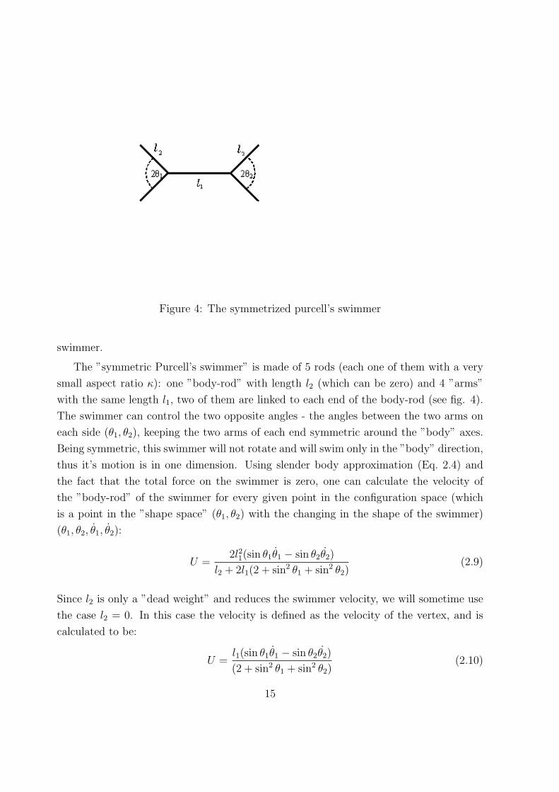
Figure 4: The symmetrized purcell’s swimmer

swimmer.

The ”symmetric Purcell’s swimmer” is made of 5 rods (each one of them with a very

small aspect ratio κ): one ”body-rod” with length l2 (which can be zero) and 4 ”arms”

with the same length l1, two of them are linked to each end of the body-rod (see fig. 4).

The swimmer can control the two opposite angles - the angles between the two arms on

each side (θ1, θ2), keeping the two arms of each end symmetric around the ”body” axes.

Being symmetric, this swimmer will not rotate and will swim only in the ”body” direction,

thus it’s motion is in one dimension. Using slender body approximation (Eq. 2.4) and

the fact that the total force on the swimmer is zero, one can calculate the velocity of

the ”body-rod” of the swimmer for every given point in the configuration space (which

is a point in the ”shape space” (θ1, θ2) with the changing in the shape of the swimmer)

(θ1, θ2, θ1, θ2):

U =2l21(sin θ1θ1 − sin θ2θ2)

l2 + 2l1(2 + sin2 θ1 + sin2 θ2)(2.9)

Since l2 is only a ”dead weight” and reduces the swimmer velocity, we will sometime use

the case l2 = 0. In this case the velocity is defined as the velocity of the vertex, and is

calculated to be:

U =l1(sin θ1θ1 − sin θ2θ2)

(2 + sin2 θ1 + sin2 θ2)(2.10)

15

As in the case of φ in the Purcell’s swimmer, we can write:

∆X =

∮

γ

Udt =

∮

γ

A1(θ1, θ2)dθ1 + A2(θ1, θ2)dθ2 =

∫

S(γ)

Fdθ1dθ2 (2.11)

where S(γ) is the oriented surface whose boundary is γ, and F = ∇∧A is called ”curvature

field” [30] and is given by:

F =−8l1sinθ1sinθ2(cosθ1 + cosθ2)

(l2 + 2l1(2 + sin2θ1 + sin2θ2))2(2.12)

and in the case l2 = 0 by:

F =−2l1sinθ1sinθ2(cosθ1 + cosθ2)

(2 + sin2θ1 + sin2θ2)2

For any curve γ in the shape space (θ1, θ2), the displacement is given by the surface

integral Eq. (2.11). As in the case of φ of the Purcell’s three linked swimmer, F (θ1, θ2)

(plotted in the background of fig. 5) contains all the information about the displacement

∆X of any stroke of this swimmer.

2.4 The most efficient stroke

In the following section we will calculate only the case l2 = 0 for simplicity, since it is clear

that this is the optimal swimmer. Looking at F in the background of Fig. (5) one can tell

immediately that the stroke for which the displacement is maximal [6], is the triangle in

shape space who’s vertices are at (0, 0); (0, π); (π, 0), and is a ”boundary stroke”, which

cannot be analyzed using slender body approximation [5] to first order.

In order to find the most efficient stroke (which is a more common way to characterize

swimmers, and can be extended to many-dimensional shape space swimmers as well), we

need to have an expression for the energy dissipation. The energy dissipation of a path

γ can be calculated by integrating the power over the time of the stroke. The power is a

quadratic expression of θ1 and θ2, and using slender body approximation (Eq. 2.4) again

one can calculate that the energy dissipation for a given curve γ is given by

E =

∫

γ

1

2gabθaθbdt (2.13)

16

(summing on a,b), where gab is given by

g1,1 = 2πµlnκ

4l31(4+2 sin2 θ2−sin2 θ1)3(2+sin2 θ1+sin2 θ2)

g2,2 = 2πµlnκ

4l31(4+2 sin2 θ1−sin2 θ2)3(2+sin2 θ1+sin2 θ2)

g1,2 = g2,1 = 2πµlnκ

4l31 sin θ1 sin θ2

3(2+sin2 θ1+sin2 θ2)

(2.14)

E depends on the time parametrization of γ, but it is known that the minimal energy

dissipation is for parametrization for which the power, P = ga,bθaθb, is constant [3]. The

expression for the dissipation (Eq. 2.13) has the form of measuring distance, and thus we

will call gi,j a metric on shape space (the dissipation metric).

Consider the problem of minimizing the energy dissipation of a stroke, subject to

the constrain of fixed step size ∆X =∮

Udt. This is a standard problem in varia-

tional calculus, and is known [1] to be equivalent to maximizing the efficiency, defined

as ε =Pdrag

Pswim=

2πln κ

4l1

R

S(γ)

F (θ1,θ2)dθ1dθ2

!2

0@ R

γ(θi)

rga,b

dθadθi

dθbdθi

dθi

1A

2 [20]. Note that since one may set τ = 1 without

loss, fixing the average speed is equivalent to fixing the step size X(γ). The minimizer,

γ(t), must then either follow the boundary or solve the Euler-Lagrange equation of the

functional

Sλ(γ) =

τ∫

0

1

2ga,bθaθbdt + λ

τ∫

0

l1(sin θ1θ1 − sin θ2θ2)

(2 + sin2 θ1 + sin2 θ2)dt (2.15)

where λ is a Lagrange multiplier, and there is a summation convention on a, b. For

each initial conditions, one can find the optimal stroke by solving the Euler-Lagrange

equations of the action in Eq. (2.15). The optimal stroke is plotted in figure (5)(computed

numerically). The efficiency for this stroke is 0.0079, which is about the same as the

efficiency of the Purcell’s swimmer for rectangular strokes [3], but less then the efficiency

for general strokes [6].

2.5 Swimming in different viscosities

Till now, we assumed that the swimmer can control it’s shape directly. This may not

always the case: some artificial swimmers (and probably some biological swimmers as

well) cannot control their shape directly, but can control the changes in their shape:

they are using constant power in fixed time parametrization, so changing the viscosity

changes the stroke. For example, consider the Purcell’s three linked swimmer, made of

17

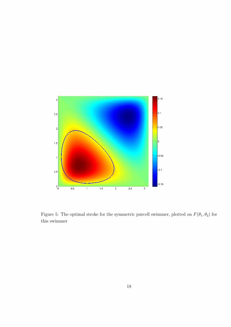
Figure 5: The optimal stroke for the symmetric purcell swimmer, plotted on F (θ1, θ2) for

this swimmer

18

Figure 6: 5-Links, A swimmer which changes its moving direction when putted in more

viscous fluid

three rods with two engines (which changes the angles between the rods), and performing

rectangular strokes (that is - the engines are working one-by-one). Now, assume that

each engine works with constant power for constant time. In this case - each engine can

change the shape of the swimmer by certain distance in shape space according to the

dissipation metric. Since the metric does depend on the viscosity, the swimmer will do

different strokes in different fluids: the more viscose the fluid, the smaller the stroke will

be. While in some cases making the stroke smaller will lead to smaller displacement, in

cases the curvature changes it sign (as in the case of Purcell’s swimmer) making smaller

strokes may lead to larger displacement.

In order to be more concrete, we will introduce another example of a symmetric

swimmer: this swimmer (which we call ”5-Links”) is again made of five rods, this time

all in a line (Fig. 6). The swimmer is symmetric around the central vertical of the middle

link, and thus can control only two angels: θ1 is the angle between the firs rod and second

one (the forth and fifth rods), and θ2 is the angle between the second and third rods (third

and forth rods). We will note the length of the first (fifth) rod as l1 (this will be our length

units), the second (forth) rod as l2 = 10l1 and the middle rod as l3 = 30l1. In order for the

arms not to collide, we will limit the shape space (θ1, θ2) to be [0.2, 2π−0.2]×[0.2, pi−0.2].

The analog for Eq. (2.12) (which is, again, not a simple expression and will not be given

here) is plotted in Fig. (7). As one can see from the figure, a stroke which is a rectangle

19

Figure 7: F (θ1, θ2) for the 5-Links swimmer

in (θ1, θ2) around (π, π2) will lead to locomotion in different directions - depending on the

amplitude of the stroke. It is clear in this case that there is some regime in which making

smaller strokes will lead to larger displacement.

The power has the following properties:

• It is quadratic in θ1,2, and can again be written as P = ga,bθaθb. ga,b can be thought

of as a metric on shape space.

• It is symmetric around θ1 = π and θ2 = π2. Thus a rectangular power stroke, that is

- a stroke in which θ1 and θ2 are changed one by one, and the power for each change

is constant for a constant time, is also a rectangle in shape space (provided it starts

from a point on the curve in shape space).

• The power is linear in µ, so changing the viscosity of the fluid will change the

amplitude of the stroke.

If we will fix the power of the engines changing θ1,2 so that in some fluid with viscosity

µ0 the stroke is symmetric around (π, π2) and will cover equal amount of negative and

positive F (θ1, θ2), putting the swimmer in more viscous fluid (µ > µ0) will lead to a

larger displacement, at least for some values of µ.

20

3 Swimming, Pumping and Gliding at low Reynolds

number

3.1 Introduction

Low Reynolds numbers hydrodynamics governs the locomotion of tiny natural swimmers

such as micro-organisms and tiny artificial swimmers, such as microbots. It also governs

micro-pumps [26], tethered swimmers [7, 27] and gliding under the action of external

forces. Our purpose here is to discuss some interesting consequences of simple, yet general

and exact relations that relate pumping, swimming and gliding at low Reynolds numbers.

The equations are not new, and appear for example in [31, 28], where they serve to analyze

swimming at low Reynolds numbers. The interpretation of these equations as a relation

between three apparently different objects: Swimmers, pumps and gliders, gives them a

new and different flavor and suggests new applications which we explore below.

Our first tool is Eq. (3.16) which relates the velocity of a free swimmer to the (torque

and) force needed to anchor it to a fixed location. This equation appears in the analysis

of swimmers [31, 28]. It can be applied to experiments on tethered swimmers [4, 16, 32]

where it can be used to infer the velocity of a free swimmers from measurements of the

force on tethered one (and vice versa) and when both are measured, to an estimate of the

gliding resistance matrix M of Eq. (3.18).

Our second tool is Eq. (3.22) which says that the power needed to operate a pump

— a tethered swimmer — is the sum of the power invested by the corresponding free

swimmer, and the power needed to tow it. (The result holds for arbitrary container of

any shape or size). It is useful in studying and comparing the efficiencies of swimmers

and pumps. In particular, it says that a tethered swimmer spends more power than a free

swimmer. As we shall see it also implies that it is impossible to pump with arbitrary high

efficiency.

Physically, both relations may be viewed as an expression of the elementary observa-

tion that swimmers and pumps are the flip sides of the same object: A tethered swimmer

is a pump [7] and an unbolted pump swims. This observation plays limited role in high

Reynolds numbers, because it does not lead to any useful equations for the non-linear

Navier Stokes equations. For microscopic objects, where the equations reduce to the

linear Stokes equations, the observation translates to linear relations.

Formally, a pump is a swimmer with a distinguished point — the point of anchoring.

The pump may have different properties depending on the point of anchoring, (we shall

21

see an example where it pumps in different directions depending on the anchoring point).

We shall solve a problem, posed by E. Yariv [31], of how to find the optimal anchoring

point for a certain class of swimmers, which we call “linear swimmers”. The class includes

the Purcell swimmer [23], the “three linked spheres” [10] and pushmepullyou [2].

There are various notions of optimality that one needs to consider in the study of

swimmers and pumps. For swimmers, one notion of optimality is to maximize the distance

covered in one stroke. A different notion is to minimize the dissipation in covering a given

distance at a given speed. Similarly, for a pump one may want to maximize the momentum

transfer to the fluid in one stroke, or, alternatively, to minimize the dissipation for given

total momentum transfer and rate. How are optimal swimmers related to optimal pumps?

We study this question for helices and show that optimal swimmers and pumps have

different geometry: There are four optimal pitch angles depending on what one optimizes

and whether the helix is viewed as a swimmer or a pump.

3.2 Anchoring as a choice of gauge

Let us start by briefly discussing the gauge issues that arise when considering swimming

[30], pumping and gliding.

Fixing a gauge is already an issue for a glider. A glider is a rigid body undergoing

an Euclidean motion under the action of an external force. There is no canonical way

to decompose a general Euclidean motion into a translation and a rotation [18]. Such a

decomposition requires choosing a fiducial reference point in the body to fix the transla-

tion. In the theory of rigid body a natural choice is the center of mass. This is, however,

not a natural choice at low Reynolds number. This is because this is the limit when

inertia plays no role and the glider may be viewed as massless. Since the choice becomes

arbitrary, it may be viewed as a choice of gauge.

In the case of a swimmer one needs to fix a point arbitrarily and in addition, to fix

a fiducial frame. This is because a swimmer is a deformable body and such a frame is

required to fix the rotation [30]. This is, again, a choice of gauge.

A pump is an anchored swimmer with a distinguished point and a distinguished frame

which are determined by the way the pump is anchored. When we write equations that

involve swimmers, pumps and gliders, we pick the fiducial point and frame determined

by the the way the pump is anchored.

22

3.3 Triality of swimmer pumps and gliders

Capital bold letters will be used for 6 dimensional vectors, non-bold Capital letters for 3

dimensional vectors and bold non-Capital letters for 3 dimensional vector fields.

We shall first recall the derivation of the linear relation between the 6 dimensional

force-torque vector, ~Fp = ( ~Fp, ~Np) which keeps a pump anchored with fixed position

and orientation, and the 6 dimensional velocity–angular-velocity vector, ~Vs = ( ~Vs, ~ωs)

associated with the corresponding autonomous swimmer:

~Fp = −M ~Vs, (3.16)

This holds for all times (~Fp,M and ~Vs are time dependent quantities). M is a 6 × 6

matrix of linear-transport coefficients of the corresponding glider:

~Fg = M ~Vg (3.17)

namely, the corresponding rigid body, moving at (generalized) velocity ~Vg under the

action of the (generalized) force ~Fg. Note the change in sign. The matrix M depends on

the geometry of the body. It is a positive matrix of the form [12]:

M =

K C

Ct Ω

(3.18)

where K,C, and Ω are 3 × 3 real matrices. Note that Eq. (3.17) fails in two dimensions

[17].

Eq. (3.16) follows from the linearity of the Stokes equations and the no-slip boundary

conditions. Let ∂Σ denote the surface of the device. Any vector field on ∂Σ can be

decomposed into a deformation and a rigid body motion as follows: Any rigid motion is

of the form ~vg = ~V + ~ω × ~x. Pick ~V to be the velocity of a fiducial point and ~ω the

rotation of the fiducial frame. The deformation field is then, by definition, what remains

when the rigid motion is subtracted from the given field ~v.

Now, decompose ~vs the velocity field on the surface of a swimmer, to a deformation

and rigid-motion as above. The deformation field can be identified with the velocity field

at the surface of the corresponding pump ~vp since the pump is anchored with the fiducial

frame that neither moves nor rotates. The remaining rigid motion ~vg is then naturally

identified with the velocity field on the surface of the glider. The three vector fields are

then related by

~vs = ~vp + ~vg, ~vg = ~Vs + ~ωs × ~x (3.19)

23

where ~Vs is (by definition) the swimming velocity and ~ωs the velocity of rotation.

Each of the three velocity fields on ∂Σ, (plus the no-slip zero boundary conditions

on the surface of the container, if there is one), uniquely determine the corresponding

velocity field and pressure (~v, p) throughout the fluid. The stress tensor, πij, depends

linearly on (~v, p) [17] .

By the linearity of the Stokes and incompressibility equations Eq. (1.2), it is clear

that ~vs = ~vg + ~vp and ps = pg + pp and then also πs = πp + πg. Since Fi =∫

∂ΣπijdSj is

the drag force acting on the device we get that the three force vectors are also linearly

related: ~Fs = ~Fp + ~Fg, and similarly for the torques. This is summarized by the force-

torque identity ~Fs = ~Fp + ~Fg. Since the force and torque on an autonomous Stokes

swimmer vanish, Eq. (3.16) follows from Eq. (3.17).

Eq. (3.16) has the following consequences:

• Micro-Pumping and Micro-Stirring is geometric: The momentum and angular mo-

mentum transfer in a cycle of a pump,∫

~Fpdt, is independent of its (time) parametriza-

tion. In particular, it is independent of how fast the pump runs. This is because

swimming is geometric [23, 30] and the matrix M is a function of the pumping cycle,

but not of its parametrization.

• Scallop theorem for pumps: One can not swim at low Reynolds numbers with self-

retracing strokes. This is known as the “Scallop theorem” [23]. An analog for

pumps states that there is neither momentum nor angular momentum transfer in a

pumping cycle that is self-retracing. This can be seen from the fact that ~Vs dt is

balanced by −~Vs dt when the path is retraced, and this remains true for M ~Vs dt.

We shall now derive an equation, originally due to [28], which relates the power ex-

penditure of swimmers, pumps and gliders. It follows from Lorentz reciprocity for Stokes

flows, discussed at section 1.3, that says that if (vj, πjk) and (v′j, π′jk) are the velocity and

stress fields for two solutions of the Stokes equations in the domain Σ then [12]:∫

∂Σ

v′i πij dSj =

∫

∂Σ

vi π′ij dSj (3.20)

For the problem at hand, we may take ∂Σ to be the surface of our device (since the

velocity fields vanish on the rest of the boundary associated with the container). The area

element ~dS is chosen normal to the surface and pointing into the fluid. Now apply the

Lorentz reciprocity to a pump and a swimmer velocity fields and use Eq. (3.19) on both

sides. This gives

−Ps + ~Vs · ~Fs = −Pp − ~Vs · ~Fp (3.21)

24

where Ps is the power invested by the swimmer and Pp the power invested by the pump.

Since the force and torque on the swimmer vanish, ~Fs = 0, we get, using Eq. (3.16) a

linear relation between the powers:

Pp − Ps = −~Vs · ~Fp = ~Vs ·M ~Vs = Pg ≥ 0 (3.22)

Pg is the power needed to tow the glider. Since both swimming and towing require positive

power, at any moment pumping is more costly than swimming or dragging1.

The linearity of Eq. (3.22) is a noteworthy, and somewhat unexpected. Eq. (3.19) says

that the corresponding velocity fields are linearly related. Since power at low Reynolds

number is quadratic in the velocity a linear relation between the powers is not what one

may naively expect.

The most interesting consequence of this relation which, at least for us, was somewhat

of a surprise, is that a pumps needs more power than a swimmer and so the power

consumed by a tethered swimmer is actually an upper bound on the power consumed by

it when freed.

One of the remarkable facts about low Reynolds number swimming is that even though

the dynamics is governed by dissipation it is still possible to swim with arbitrarily high

efficiency [2, 19]. For this to happen, the swimming velocity should be non-zero, but the

energy dissipation of the swimmer, Ps, should be zero, thus Pp = Pg ≥ 0. The same

cannot happened for pumps: for a pump to be with arbitrarily high efficiency, it must

have non-zero momentum transfer to the fluid and zero power. Since M of Eq. (3.18)

is a strictly positive matrix Pg is quadratic in the force and can not vanish if the pump

transfers momentum to the fluid.

3.4 Linear swimmers and optimal anchoring

E. Yariv [31] posed the following problem: Find the anchoring point which optimizes the

momentum transfer to the fluid. The general case is complicated. A class of swimmer for

which this question can be answered relatively easily is the class of “linear swimmers” —

swimmers made of segments, so that the velocity of different points on the same segment

depend linearly on the distance between the points. This class contains the three linked

spheres [10], the pushmepullyou [2], Purcell’s three linked swimmer [3, 6], the ‘N-Linked’

swimmer [8], but not, for example, the treadmiller [19].

1In the case that the pump is allowed to rotate M is replaced by K and ~Vs by ~Vs .

25

Figure 8: A treadmiller transports its skin from head to back. The treadmiller in the

figure swims to the left while the motion of its skin guarantees that,in the limit of large

aspect ratio, the ambient fluid is left almost undisturbed. If it is anchored at the gray

point then it transfers momentum to the fluid (to the right). The power of towing a frozen

treadmiller and of pumping almost coincide reflecting the fact that a treadmiller swims

with little dissipation.

Shifting the anchoring point by ~r, the resistance matrixes K, C and Ω of Eq. 3.18 will

be changed to Kr = K, Cr = C −KR and Ωr = Ω − RKR + CR − RCt [12], where R

is the antisymmetric matrix associated with the vector ~r. The change in ~Vs is linear in

~r, and ~ωs is unchanged [18]. Using Eq. (3.16), the change in the force ~Fp (and hence in

the linear-momentum transfer to the fluid) is linear with ~r, and the optimal point which

maximized the force must be at one of the edges of the segments.

(The change in the torque ~Tp (and hence in the angular-momentum transfer to the

fluid) is quadratic in ~r, so the maximum can be either at the edges, or at the point in

which the differential of the angular momentum with respect to the anchoring point is

zero (in cases where there is such a point). In either case, one has to check only a few

points.)

A case in point is the “three linked spheres” [10]. There are three candidates for

the optimal anchoring point: The three spheres. The two outer spheres are related by

symmetry so the two interesting cases are either anchoring on an outer sphere or in the

middle sphere. Detailed calculations show (appendix A) that the maximum momentum

transfer will be when the anchoring point is on one of the outer spheres. When the

swimmer is anchored on the middle sphere, the momentum transfer turns out to be in

the opposite direction. Calculation for the efficiency shows that the optimal point in this

case is also at the outer spheres.

26

3.5 Helices as swimmers and pumps

Eq. (3.16) and Eq. (3.22) have an analogs for non-autonomous rigid swimmers such as a

helix rotating by the action of an external torque [25]. This is a case that is very easy to

treat separately. From Eq. (3.17) applied to the helix twice, once as swimmer and once

as a pump we get the analog of Eq. (3.16):

~Fp = C~ω = −K~Vs (3.23)

The analog of Eq. (3.22) follows immediately from the definition of the power P = −~F · ~Vand Eq. (3.17) again:

Pp − Ps = ~Fp · ~Vp − ~Fs · ~Vs = −~Vs · ~Fp = Pg (3.24)

It follows from this that the difference in power between a swimmer and a pump is

minimized, for given swimming velocity, if the swimming direction coincides with the

smallest eigenvalue of K which is the direction of optimal gliding.

The distinction between optimal pumps and optimal swimmers [24] can be nicely

illustrated by the considering the example of a rotating helix, or a screw. This motion

has been studied carefully in [20, 13] whose analysis goes beyond what we need here.

For a thin helix the slender-body theory [5], discussed earlier in section 2.2, can be used.

Consider a helix of radius r, pitch angle θ and total length `. The helix is described by

the parameterized curve

(r cos φ, r sin φ, t sin θ), φ =t

rcos θ, t ∈ [0, `] (3.25)

Suppose the helix is being rotated at frequency ω about its axis. Substituting the velocity

field of a rotating helix, with an unknown swimming velocity in the z-direction, into

Eq. (2.4), and setting the total force in the z-direction to zero, fixes the swimming velocity.

Dotting the force with the velocity and integrating gives the power. This slightly tedious

calculation gives for the swimming velocity (along the axis) and the power of swimming:

Vs

ωr=

sin 2θ

3 + cos 2θ,

Ps

k`ω2r2=

4

3 + cos 2θ(3.26)

Similarly, for the pumping force and power one finds

Fp

k`ωr= sin θ cos θ,

Pp

k`ω2r2= 1 + sin2 θ (3.27)

Eq. (3.26) and (3.27) have the following consequences for optimizing pumps and swimmers:

27

• Given ωr, a swimmer velocity Vs is maximized at pitch angle θ = 54.74.

• Given ωr, the pumping force Fp is maximized at θ = 45.

Consider now optimizing both the pitch angle θ and rotation frequency ω so that the

swimming velocity is maximized for a given power. Namely

maxθ,ω

Vs | Ps = const (3.28)

and similarly for pumping, except that Fp replaces Vs and Pp replaces Ps. A simple

calculation shows that this is equivalent to optimizing V 2s /Ps and F 2

p /Pp with respect to

θ. (These ratios are independent of ω and so invariant under scaling time). One then

finds:

• The efficiency of swimming, V 2s /Ps, is optimized at θ = 49.9. The efficiency is

proportional to (k`)−1 which favors small swimmers in less viscous media, as one

physically expects.

• The efficiency of pumping, F 2p /Pp, is optimized at θ = 42.9. The efficiency is

proportional to (k`) which favors big pumps at more viscous media. Micro-pumps

are perforce inefficient.

There is a somewhat unrelated, yet insightful fact that one learns from the above

computation regarding the difference between motion in a very viscous fluid and motion

in a solid. The naive intuition that the two are similar at very high viscosity would imply

that a helix moves like a cork-screw and so would move one pitch in one turn. This is

actually never the case, no matter how large µ is. In fact, the ratio of velocities of a helix

to a cork-screw is independent of µ and by Eq. (3.26)

Vs

ωr sin θ=

cos θ

1 + cos2 θ≤ 1

2(3.29)

A helix needs at least two turns to advance the distance of its threads.

3.6 Pumps that do not swim

We have noted that the “three linked spheres” can pump either to the right or to the left

depending on whether it is anchored on the center sphere or on an external sphere. There

is, therefore, an intermediate point where it will not pump.

28

θ

θ1

2

Figure 9: A Purcell three linked swimmer, left, controls the two angles θ1 and θ2. When

bolted it effectively splits into two independent wind-shield wipers each of which is self

retracing. It will, therefore, not pump. Pushmepullyou, right, controls the distance

between the two spheres and the ratio of their volumes. It can have arbitrarily large

swimming efficiency.

There are also pumps that will not swim: Evidently, if the swimming stroke is right-

left and up-down symmetric, the swimmer will not move by symmetry. It can, however,

be bolted in a way that breaks the symmetry to give an effective pump. For example

- consider a right-left symmetric pushmepullyou [2], where the two spheres inflate and

deflate in phase. By symmetry, it will not swim, however, anchoring in any point except

the middle point will lead to net momentum transfer.

29

30

4 Summary

Swimming at low Reynolds number is geometric [30]. E. M. Purcell, who was the first

to point this out[23], invented a very simple swimmer, made of three link (see Fig. 1),

to emphasize the geometric nature of swimming at low Reynolds number. In this work

we explore this swimmer using geometric tools. Although this point of view does not

lead to any analytical expression which helps us understanding this swimmer better, it

does let us to visualize how the swimmer will behave in the small strokes regime, and

how approximately it will behave in large strokes as well (see Fig. (2) and Fig. (3)).

This visualization tools can help us in searching for the optimal strokes [22, 6], and can

explain some ”wired” behavior of the swimmer, like the fact that it swims in different

directions when the amplitude of the stroke changes [3]. Since this swimmer turns out to

be very complicated to analyzed, we introduce a much simpler swimmer, made of 5 rods,

which is in some sense a ”symmetrization” of the original Purcell’s three linked swimmer.

Being symmetric, this swimmer cannot rotate, and calculating analytically his velocity,

locomotion per stroke and energy dissipation, is very easy. This let us find the optimal

stroke for this swimmer.

In many cases, a swimmer cannot control it’s shape directly, but only the power he

used to change it’s shape. In such cases, the swimming will be medium dependent: the

energy dissipation of the swimmer form a metric on shape space. This metric depends

on the viscosity of the fluid, so the swimmer will do different strokes in different fluids:

the swimmer is performing a stroke with a fixed length in the dissipation metric. This

definition of a stroke can lead to a swimming with larger displacement in more viscose

fluid, which is the case in a new swimmer (the ”5-Links”) we introduce. The motivation

for this definition is a micro-organism, Spiroplasma [9], who is known to swim better in

more viscose fluids. The actual reason for the Spiroplasma to swim better in more viscose

fluid is unknown, and the ”5-Links” swimmer shows one model this might happened.

After studying swimmers, we turn to studying the relations between a swimmer and

the pump one would get by anchoring the swimmer. The motivation for this research is

the experimental simplicity of measuring anchored swimmer instead of free ones, and the

need for pumps for micro-fluid devices. In order to relate swimmers to pump we use the

linearity of the Stokes equation, and the Lorenz reciprocity. The relations we get for the

force–velocity and the powers are very simple, and relate pumps to swimmers through a

glider - which is a frozen swimmer dragged by an external force. They say that a pump

will always use more power then the swimmer, and shed light on why it is possible to

swim with arbitrarily low energy cost but it is impossible to pump with arbitrarily low

31

energy cost.

We give some examples to the use of the relations between pump and swimmer: we

answer the question of ”Where to anchor a given swimmer to get the pump with largest

momentum transfer” for a class of swimmer we call ”linear swimmers” which include

many of the swimmers like the Purcell’s three linked swimmer, the three linked spheres,

the Pushmepullyou and the N-linked swimmer. We calculate the pitch angle for a helix in

the case of pump and a swimmer, optimizing the velocity, force, and efficiency. We get 4

different pitches for the 4 cases. We end up by showing that there are cases of a swimmer

that will not pump and a pump that will not swim.

32

A The three linked swimmer as a pump

The three linked spheres [10], is a simple swimmer made of three spheres with radiuses a in

a line, located at x1, x2 = x1 +q1, x3 = x2 +q2, which can control the two distances q1 and

q2. This swimmer can be analyzed using the Oseen tensor (which is a good approximation

for the case qi >> R; i = 1, 2): the force on the i sphere is given by [12]:

Fi =3∑

j=1

HijVj with

Hii = −6πµa

Hij = −6πµa 3RXij

Xij = |xi − xj|(A.30)

The total momentum transferred to the fluid in one stroke can be calculated by in-

tegrating3∑

i=1

Fi over a complete stroke cycle. The total momentum transfer is invariant

under changes in the time parametrization: ∆Momentum =∫ 3∑

i=1

Fidt =∫ 3∑

i,j=1

Hijdxj.

Here we will analyze this swimmer for the simple case of rectangular strokes: we start

with q1 = q2 = q, and in the strokes we change q1 to be q + ∆q, then q2 to be q + ∆q,

then changing q1 back to q and then changing q2 to q. When anchoring the swimmer in

one of the outer spheres (the left one, in this example), the total momentum transfer for

the stroke is given (calculating the integral over the stroke using Mathematica) by:

−18πa2∆q2

q(q + ∆q)

which is a negative expression, corresponding the fact that the momentum transfer is to

the left. When anchoring the swimmer at the middle sphere, the total momentum transfer

for the stroke is given (calculating the integral over the stroke using Mathematica) by :

−18πa2 ln

(4q(q + ∆q)

4q(q + ∆q) + ∆q2

)

Since the denominator in the ln is grater than the numerator, the sign of the ln is negative,

and this expression is positive: the total momentum transfer in this case is to the right!

33

34

References

[1] J. E. Avron, O. Gat, and O. Kenneth. Optimal swimming at low reynolds numbers.

Physical Review Letters, 93(18):186001, 2004.

[2] J. E. Avron, O. Kenneth, and D. H. Oaknin. Pushmepullyou: an efficient micro-

swimmer. New Journal of Physics, 7:234–242, 2005.

[3] L. E. Becker, S. A. Koehler, and H. A. Stone. On self-propulsion of micromachines at

low reynolds number: Purcell’s three-link swimmer. J. of Fluid Mechnics, 490:15–35,

2003.

[4] S. Chattopadhyay, R. Moldovan, C. Yeung, and X. L. Wu. Swimming efficiency of

bacterium escherichia coli. PNAS, 103(13):13712–13717, September 2006.

[5] R.G. Cox. The motion of long slender bodies in a viscous fluid part 1. general theory.

J. Fluid Mechanics, 44(4):791–810, December 1970.

[6] A. E. Hosoi D. Tam. Optimal stroke patterns for purcell’s three-linked swimmer.

Physical Review Letters, 98:4, February 2007.

[7] Nicholas Darnton, Linda Turner, Kenneth Breuer, and Howard C. Berg. Moving

fluid with bacterial carpets. Biophysical Journal, 86(4):1863, 2004.

[8] Gerusa Alexsandra de Araujo and Jair Koiller. Self-propulsion of n-hinged ’animals’

at low reynolds number. QUALITATIVE THEORY OF DYNAMICAL SYSTEMS,

4(58):139–167, 2004.

[9] Trachtenberg S. Gilad R., Porat A. Motility modes of spiroplasma melliferum

bc3: ahelical, well-less bacterium deriven by linear motor. Molecular Micribiology,

47(3):657–669, February 2003.

[10] R. Golestanian and A. Najafi. Simple swimmer at low reynolds number: Three linked

spheres. Phys. Rev. E, 69:062901–062905, 2004.

[11] R. R. Netz H. Wada. Model for self-propulsive helical filaments: Kink-pair propaga-

tion. Phys. Rev. Lett, 99:108102–1:4, September 2007.

[12] J. Happel and H. Brenner. Low Reynolds number hydrodynamics. Kluwer, second

edition, 1963.

35

[13] J. J. L. Higdon. The hydrodynamics of flagellar propulsion: helical waves. J. Fluid

Mechanics, 94(02):331–351, September 1979.

[14] M. Draper R. T. Kelly A. T. Woolley J. W. Munyan, H.V. Fuentes. Electrically

actuated, pressure-driven microfluidic pumps. Lab on a Chip Comm., 3:217–220,

2003.

[15] H. C. Berg R. Montgomery K. M. Ehlers, A. D. T. Samuel. Do cyanobacteria swim

using traveling surface waves? Proc. Natl. Acad. Sci., 93:8340–8342, August 1996.

[16] G. Kosa, M. Shoham, and M. Zaaroor. Propulsion of a swimming micro medical

robot. Robotics and Automation, 2005.

[17] L. D. Landau and I. M. Lifshitz. Fluid Mechanics. Pergamon, 1959.

[18] L. D. Landau and I. M. Lifshitz. Mechanics. Butterworth and Heinemann, 1981.

[19] A.M. Leshansky, O. Kenneth, O. Gat, and J.E. Avron. A frictionless microswimmer.

New J. Phys., 2007.

[20] J. Lighthill. Mathematical Biofluid-dynamics. Society of Industrial and Applied

Mathematics, 1975.

[21] J. Baudry M. Fermigier J. Bibette H. A. Stone M. Roper, R. Dreyfus. On the

dynamics of magnetically driven elastic filaments. J. Fluid Mechanics, 554:167–190,

2006.

[22] J. E. Avron O. Raz. A comment on ”optimal stroke patterns for purcell’s three-linked

swimmer”. Phys. Rev. Lett, in preprint.

[23] E. M. Purcell. Life at low reynolds number. American Journal of Physics, 45(1):3–11,

January 1977.

[24] M. E. Purcell. The efficiency of propulsion by a rotating flagellum. PNAS,

94:1130711311, October 1997.

[25] Dreyfus R., Baudry J., Roper M. L., Fermigier M., Stone H. A., and Bibette J.

Microscopic artificial swimmer. Nature, 436:862–865, 2005.

[26] 2000 R. F. Day, H. A. Stone :. Lubrication analysis and boundary integral simulations

of a viscous micropump. J. of Fluid Mechanics, 416:197–216, 2000.

36

[27] K. Levit-Gurevich S. Gueron. Energetic considerations of ciliary beating and the

advantage of metachronal coordination. PNAS, 96:12240–12245, October 1999.

[28] Samuel A. D. T Stone H. A. Propulsion of microorganisms by surface distortions.

Phys. Rev. Lett., 77(19):4102–4104, November 1996.

[29] G. I. Taylor. Analysis of the swimming of microscopic animals. Proc. R. Soc. Lond.

A, 209:447461, 1951.

[30] F. Wilczek and A. Shapere. Geometry of self-propulsion at low reynolds number. J.

of Fluid Mechanics, 198:557–585, 1989.

[31] E. Yariv. Self-propulsion in a viscous fluid: arbitrary surface deformations. J. Fluid

Mechanics, 550:139148, 2006.

[32] Tony S. Yu, Eric Lauga, and A. E. Hosoi. Experimental investigations of elastic tail

propulsion at low reynolds number. arXiv:cond-mat/0606527, 2006.

37