Embed Size (px)
Citation preview

i
Modeling and Simulation of
Electromagnetic Damper to
Improve Performance of a Vehicle
during Cornering
by
Saad Bin Abul Kashem
A Thesis Submitted to the Swinburne University of Technology In Fulfillment of the
Requirements for the Degree of PhD
in the Faculty of Engineering and Industrial Sciences
Saad Bin Abul Kashem, 2013 Swinburne University of Technology
Hawthorn, Melbourne, VIC 3122

ii
Author's declaration
This is to certify that the thesis submitted to the Swinburne University of
Technology for the award of the degree of Doctor of Philosophy. The contents of
this thesis, in full or in parts, have not been submitted to any other Institute or
University for the award of any degree or diploma. I hereby declare that I am the
sole author of this thesis. To the best of my knowledge, the thesis contains no
material previously published or written by another person except where due
reference is made in the text.
Saad Bin Abul Kashem

iii
Abstract
A suspension system is an essential element of a vehicle to isolate the frame of
the vehicle from road disturbances. It is required to maintain continuous contact
between a vehicle’s tyres and the road. In order to achieve the desired ride
comfort, road handling performance, many researches has been conducted. A
new modified skyhook control strategy with adaptive gain that dictates the
vehicle’s semi-active suspension system is presented. The proposed closed loop
feedback system first captures the road profile input over a certain period. Then it
calculates the best possible value of the skyhook gain for the subsequent process.
Meanwhile the system is controlled according to the new modified skyhook
control law using an initial or previous value of the skyhook gain. In this
research, the proposed suspension system is compared with passive and three
other recently reported skyhook controlled semi-active suspension systems
through a virtual environment with MatLab/SIMULINK as well as an
experimental analysis with Quanser suspension plant. Its performances have been
evaluated in terms of ride comfort and road handling performance. The model
has been validated in accordance to the international standards of admissible
acceleration levels ISO2631 and human vibration perception. This control
strategy has also been employed on the full car model to improve the isolation of
the vibration and handling performance of the road vehicle.
This thesis also describes the development of a new analytical full vehicle
model with nine degrees of freedom, which uses the new modified skyhook
strategy to control the full vehicle vibration problem. Nowadays, many
researchers are working on active tilting technology to improve vehicle
cornering. But in those work, the effect of road bank angle is not considered in
the control system design or in the dynamic model of the tilting standard
passenger vehicles. The non-incorporation of road bank angle creates a non-zero
steady state torque requirement. Therefore, in this research this phenomenon was

iv
addressed while designing the direct tilt control and the dynamic model of the
full car model.
This research has indicated the potential of the SKDT suspension system
in improving cornering performances of the vehicle and paves the way for future
work on vehicle’s integrated system for chassis control.
Key words: quarter-car, vehicle, suspension, semi-active, skyhook,
adaptive, control, damper, Quanser.

v
Acknowledgements
It is a pleasure to thank all the people who made this thesis possible. It is
impossible to overstate my gratitude to my supervisors, Dr. Mehran Ektesabi and
Prof. Romesh Nagarajah from the Faculty of Engineering & Industrial Sciences
of Swinburne University of Technology with their enthusiasm, their inspiration,
and their great efforts in explaining things clearly and simply which helped to
make the thesis fun for me. Throughout my thesis-writing period, they provided
me with encouragement, sound advice, good teaching, good company, and lots of
good ideas.
It is my great pleasure to offer warm thanks to Professor Saman
Halgamuge who is the Assistant Dean of Melbourne School of Engineering at
The University of Melbourne. The effort and time he took to help me to validate
the designed full car analytical model was outstanding.
As a graduate student, I have had the honour of attending many lectures
and courses at Swinburne University of Technology; in particular, I enjoyed and
learned much from attending lectures by Dr. Zhenwei Cao and Prof Zhihong
Man. I have attended Control and Automation, Robotic Control and Advanced
Mechatronics.
Over the last three years, I have been privileged to work with and learn
from and Timothy Barry and Mehedi Al Emran Hasan. They helped me to learn
MatLab/Simulink. I am also grateful to them for helping me to get through the
difficult times, and for all the emotional support.
It is my pleasure to thank Jason Austin, Simon Lehman and Alex Barry
who worked with me to setup and experiment the Quanser Suspension Plant.
From my supervision of their Undergraduate Final Year Project on active
suspension system, I have learned many things.

vi
I wish to thank Dr. Durul Huda for his time and patience in teaching me
about the dynamics of the full car model.
I would like to thank the many people who have taught me Science: my
high school teachers (especially Abdul High) and my undergraduate faculties at
East West University (especially Md. Ishfaqur Raza PhD, Dr. Ruhul Amin, Dr.
Anisul Haque, Dr. Mohammad Ghulam Rahman, Dr. Khairul Alam, Dr. Tanvir
Hasan Morshed), for their wise advice, helping with various applications, and so
on.
Lastly, and most importantly, I wish to thank my two sisters Ishrat
Kashem, Rumana Kashem and in laws Sanjar Iqbal Khan, Fazley Rabbi, my
parents, Syeda Nazma Kashem and Md. Abul Kashem and my wife Humaira
Rashid. They supported me and loved me. To them I dedicate this thesis.
And special thanks to almighty Allah to made this thesis possible.

vii
Table of Contents Author's declaration ............................................................................................... ii
Abstract ................................................................................................................. iii
Acknowledgements ................................................................................................. v
Table of Contents ................................................................................................. vii
List of Figures ........................................................................................................xi
List of Tables ..................................................................................................... xvii
Chapter 1 Introduction ............................................................................................ 1
1.1 Background ................................................................................................... 1
1.2 Research motivation and methodologies ....................................................... 6
1.3 Outline of the thesis ....................................................................................... 9
Chapter 2 Literature review .................................................................................. 12
2.1 Overview ..................................................................................................... 12
2.2 Control strategies ......................................................................................... 12
2.2.1 Linear Quadratic Regulator & Linear Quadratic Gaussian .................. 14
2.2.2 Sliding mode control ............................................................................. 16
2.2.3 Fuzzy and neuro-fuzzy control ............................................................. 18
2.2.4 Skyhook control method ....................................................................... 20
2.2.5 Groundhook control method ................................................................. 24
2.3 Active tilting technology ............................................................................. 25
2.3.1 Narrow titling road vehicle: .................................................................. 25
2.3.2 Tilting standard production vehicle ...................................................... 30
2.4 Conclusion ................................................................................................... 32
Chapter 3 Vehicle suspension system ................................................................... 33
3.1 Overview ..................................................................................................... 33
3.2 Vehicle suspension system .......................................................................... 33
3.2.1 Passive suspension system .................................................................... 34
3.2.2 Semi-active suspension System ............................................................ 36
3.2.3 Active suspension system ..................................................................... 37

viii
3.3 Quarter-car suspension model ..................................................................... 38
3.3.1 Explanation of motion equations of quarter-car ................................... 40
3.3.2 High vs. low-bandwidth suspension system ......................................... 44
3.4 Comparison of recent models ...................................................................... 46
3.5 Conclusions ................................................................................................. 51
Chapter 4 Design of semi-active suspension system ............................................ 52
4.1 Overview ..................................................................................................... 52
4.2 Semi-active control algorithms ................................................................... 52
4.2.1 Continuous skyhook control of Karnopp et al. (1974) ......................... 53
4.2.2 Modified skyhook control of Bessinger et al. (1995) ........................... 53
4.2.3 Optimal skyhook control of Nguyen et al. (2009) ................................ 54
4.2.4 Proposed skyhook control with adaptive skyhook gain ........................ 55
4.3 Road profile description .............................................................................. 59
4.4 Comparison and evaluation using Y. Chens’ model ................................... 62
4.4.1 Comparison ........................................................................................... 64
4.4.2 Evaluation ............................................................................................. 66
4.5 Comparison and evaluation of Quanser suspension plant ........................... 68
4.5.1 Quanser quarter-car suspension plant ................................................... 68
4.5.2 Comparison ........................................................................................... 80
4.5.3 Evaluation ............................................................................................. 83
4.6 Conclusions ................................................................................................. 84
Chapter 5 Full car model cornering performance ................................................. 86
5.1 Overview ..................................................................................................... 86
5.2 Full car modelling ....................................................................................... 86
5.2.1 Semi-active suspension model .............................................................. 86
5.2.2 Vehicle tilting model ............................................................................. 89
5.3 Vehicle rollover estimation ......................................................................... 91
5.4 Controller design ......................................................................................... 93
5.4.1 Direct tilt control design ....................................................................... 93
5.5 Road profile and driving scenario ............................................................... 97

ix
5.5.1 Driving scenario one ............................................................................. 98
5.5.2 Driving scenario two ............................................................................. 99
5.5.3 Driving scenario three ........................................................................... 99
5.5.4 Driving scenario four .......................................................................... 100
5.6 Evaluation criteria ..................................................................................... 101
5.6.1 Evaluation on ride comfort performance ............................................ 101
5.6.2 Admissible acceleration level test based on ISO 2631 ....................... 102
5.6.3 Evaluation on road handling performance .......................................... 103
5.7 Conclusion ................................................................................................. 103
Chapter 6 Simulation of full car model .............................................................. 105
6.1 Overview ................................................................................................... 105
6.2 Simulation environment ............................................................................ 105
6.3 Simulation with the proposed skyhook controller..................................... 108
6.3.1 Simulation on road class A ................................................................. 108
6.3.2 Simulation on road class B ................................................................. 115
6.3.3 Simulation on road class C ................................................................. 122
6.3.4 Simulation on combined road ............................................................. 129
6.4 Simulation with skyhook and direct tilt controller .................................... 136
6.4.1 Simulation on driving scenario one .................................................... 136
6.4.2 Simulation on driving scenario two .................................................... 145
6.4.3 Simulation on driving scenario three .................................................. 154
6.4.4 Simulation on driving scenario four ................................................... 163
6.5 Simulation Summary ................................................................................. 172
6.5.1 Simulations of ride comfort in the frequency domain ........................ 173
6.5.2 Simulations of ride comfort in the time domain ................................. 177
6.6 Conclusions ............................................................................................... 188
Chapter 7 Experimental analysis of full car model ............................................ 191
7.1 Overview ................................................................................................... 191
7.2 Experimental environment ........................................................................ 191
7.3 Quanser plant at front left suspension ....................................................... 195

x
7.3.1 Experiments of ride comfort in the frequency domain ....................... 197
7.3.2 Experiments of ride comfort in the time domain ................................ 201
7.4 Quanser plant at rear right suspension ...................................................... 212
7.4.1 Experiments of ride comfort in the frequency domain ....................... 214
7.4.2 Experiments of ride comfort in the time domain ................................ 218
7.5 Conclusions ............................................................................................... 229
Chapter 8 Conclusions and recommendations .................................................... 231
8.1 Introduction ............................................................................................... 231
8.2 Overview of the study ............................................................................... 232
8.3 Recommendations for future study ........................................................... 238
References ........................................................................................................... 239
Appendix A ......................................................................................................... 248
Appendix B ......................................................................................................... 250
Appendix C ......................................................................................................... 255

xi
List of Figures Figure 1-1 Vehicle suspension system..............................................................................2 Figure 1-2 Rear suspension system without wheel of a vehicle.......................................2 Figure 1-3 The Passive, Semi-active and Active suspension system. ................................ 3
Figure 2-1. An ideal skyhook configuration. ................................................................... 21
Figure 2-2. A schematic of the Groundhook control system. ......................................... 24
Figure 2-3 Narrow commuter vehicle[106]. ................................................................... 25
Figure 2-4 (a) Vehicle tilt by suspension [107], (b) Vehicle tilt by actuator. .................26 Figure 2-5 Nissan Land Glider [35]. ................................................................................. 31
Figure 3-1 Suspension system [118]. .............................................................................. 33
Figure 3-2 Passive suspension system. ........................................................................... 34
Figure 3-3 Semi-active suspension system. .................................................................... 36
Figure 3-4 Active suspension system. ............................................................................. 37
Figure 3-6 Mass spring characteristics. ........................................................................... 40
Figure 3-7 Mass-spring-damper configuration. .............................................................. 41
Figure 3-8 Two degree of freedom horizontal multiple mass spring damper. ............... 42
Figure 3-9 Vertical multiple mass spring damper configuration. ................................... 43
Figure 3-10 Forces acting at a point. ............................................................................... 43
Figure 3-11 (a) Low-bandwidth suspension model, (b) high-bandwidth suspension model. ............................................................................................................................. 45
Figure 3-12 The road profile. .......................................................................................... 46
Figure 3-13 (a) Comparison between passive suspension models 1 to 6, (b) Comparison between passive suspension models 1 and 7 to 11. ....................................................... 48
Figure 4-1 Schematic of the suspension systems based on proposed modified skyhook control system with adaptive skyhook gain....................................................................58 Figure 4-2 (a) The time histories of three classes of roads, (b) Power spectral density of three classes of road. ...................................................................................................... 61
Figure 4-3 The time history of road profile. .................................................................... 63
Figure 4-4 The sprung mass acceleration of the passive and semi-active suspension systems. ........................................................................................................................... 63
Figure 4-5 The ride comfort performance comparison. ................................................. 65
Figure 4-6 The road handling performance comparison. ............................................... 66
Figure 4-7 Vertical vibration of car suspension in frequency domain. ........................... 67
Figure 4-8 Quanser Suspension Plant. ............................................................................ 69
Figure 4-9 Vehicle suspension system............................................................................71 Figure 4-10 The Quanser quarter-car model experimental setup. ................................. 74
Figure 4-11 The Quanser suspension plant modeled in Simulink................................... 75
Figure 4-12 DC micro motor characteristics curve[144]. ................................................ 78
Figure 4-13 The sprung mass acceleration of the passive and semi-active suspension systems (a) in simulation environment, (b) in experimental setup. ............................... 79
Figure 4-14 The ride comfort performance comparison (a) in simulation environment, (b) through experimental setup. ..................................................................................... 81
Figure 4-15 The road handling performance comparison (a) in simulation environment, (b) through experimental setup. .................................................................................... .82

xii
Figure 4-16 Vertical vibration of car suspension in frequency domain. ......................... 83
Figure 5-1 A schematic diagram of a full-vehicle active suspension system [142]......... 87
Figure 5-2 Free body diagram of a Bicycle model [31]. .................................................. 90
Figure 5-3 Stable and unstable lateral forces acting on a static vehicle [148]. .............. 92
Figure 5-4 Vehicle suspension system............................................................................95 Figure 5-5 Driving scenario one. ..................................................................................... 98
Figure 5-6 Driving scenario two. ..................................................................................... 99
Figure 5-7 Driving scenario three.................................................................................101 Figure 5-8 Driving scenario four. ................................................................................... 100
Figure 6-1 Simulink model............................................................................................107 Figure 6-2 The frequency domain response of the car body vertical acceleration to road class A: (a) at narrow frequency range and (b) at broad frequency range. ......... 109
Figure 6-3 The frequency domain response of the car body pitch angular acceleration to road class A: (a) at narrow frequency range and (b) at broad frequency range. ..... 110
Figure 6-4 The time domain response of vehicle body vertical acceleration to road class A: (a) full trajectory and (b) short time span. ............................................................... 112
Figure 6-5 The time domain response of vehicle pitch angular acceleration to road class A: (a) full trajectory and (b) short time span. ............................................................... 113
Figure 6-6 The time domain response of vehicle pitch angular acceleration to road class A: (a) full trajectory and (b) short time span. ............................................................... 114
Figure 6-7 The frequency domain response of the car body vertical acceleration to road class B: (a) at narrow frequency range and (b) at broad frequency range. ......... 116
Figure 6-8 The frequency domain response of the car body pitch angular acceleration to road class B: (a) at low frequency and (b) at broad frequency range. ..................... 117
Figure 6-9 The time domain response of vehicle body vertical acceleration to road class B: (a) full trajectory and (b) short time span. ............................................................... 119
Figure 6-10 The time domain response of vehicle pitch angular acceleration to road class B: (a) full trajectory and (b) short time span. ....................................................... 120
Figure 6-11 The time domain response of the vehicle sprung mass m1 vertical displacement to road class B: (a) full trajectory and (b) short time span. ................... 121
Figure 6-12 The frequency domain response of the car body vertical acceleration to road class C: (a) at narrow frequency range and (b) at broad frequency range. ......... 123
Figure 6-13 The frequency domain response of the car body pitch angular acceleration to road class C: (a) at narrow frequency range and (b) at broad frequency range. ..... 124
Figure 6-14 The time domain response of vehicle body vertical acceleration to road class C: (a) full trajectory and (b) short time span. ....................................................... 126
Figure 6-15 The time domain response of vehicle pitch angular acceleration to road class C: (a) full trajectory and (b) short time span. ....................................................... 127
Figure 6-16 The time domain response of the vehicle sprung mass m1 vertical displacement to road class C: (a) full trajectory and (b) short time span. ................... 128
Figure 6-17. The frequency domain response of the car body vertical acceleration to the combined road: (a) at narrow frequency range and (b) at broad frequency range. ....................................................................................................................................... 130

xiii
Figure 6-18. The frequency domain response of the car body pitch angular acceleration to the combined road: (a) at narrow frequency range and (b) at broad frequency range. ........................................................................................................... 131
Figure 6-19 The time domain response of vehicle body vertical acceleration to the combined road: (a) full trajectory and (b) short time span. ......................................... 133
Figure 6-20 The time domain response of vehicle pitch angular acceleration to the combined road: (a) full trajectory and (b) short time span. ......................................... 134
Figure 6-21 The time domain response of the vehicle sprung mass m1 vertical displacement to the combined road: (a) full trajectory and (b) short time span. ........ 135
Figure 6-22 The response of steering and bank angle in driving scenario one: (a) Desired tilting angle (b) Required actuator force. ........................................................ 137
Figure 6-23 The vehicle body vertical acceleration for driving scenario one: (a) full trajectory and (b) short time span. ............................................................................... 139
Figure 6-24 The pitch angular acceleration for driving scenario one: (a) full trajectory and (b) short time span. ................................................................................................ 140
Figure 6-25 The roll angular acceleration for driving scenario one: (a) full trajectory and (b) short time span. ....................................................................................................... 141
Figure 6-26 The lateral acceleration for driving scenario one: (a) full trajectory and (b) short time span. ............................................................................................................ 142
Figure 6-27 The vehicle sprung mass m1‘s vertical displacement for driving scenario one: (a) full trajectory and (b) short time span. ........................................................... 143
Figure 6-28 The rollover threshold in driving scenario one: (a) full trajectory and (b) short time span. ............................................................................................................ 144
Figure 6-29 The response of steering and bank angle in driving scenario two: (a) Desired tilting angle (b) Required actuator force. ........................................................ 146
Figure 6-30 The vehicle sprung mass m1‘s vertical displacement for driving scenario two: (a) full trajectory and (b) short time span. ........................................................... 148
Figure 6-31 The vehicle body vertical acceleration for driving scenario two: (a) full trajectory and (b) short time span. ............................................................................... 149
Figure 6-32 The pitch angular acceleration for driving scenario two: (a) full trajectory and (b) short time span. ................................................................................................ 150
Figure 6-33 The roll angular acceleration for driving scenario two: (a) full trajectory and (b) short time span. ....................................................................................................... 151
Figure 6-34 The lateral acceleration for driving scenario two: (a) full trajectory and (b) short time span. ............................................................................................................ 152
Figure 6-35 The rollover threshold in driving scenario two: (a) full trajectory and (b) short time span. ............................................................................................................ 153
Figure 6-36 The response of steering and bank angle in driving scenario three: (a) Desired tilting angle (b) Required actuator force. ........................................................ 155
Figure 6-37 The vehicle sprung mass m1‘s vertical displacement for driving scenario three: (a) full trajectory and (b) short time span. ......................................................... 157
Figure 6-38 The vehicle body vertical acceleration for driving scenario three: (a) full trajectory and (b) short time span. ............................................................................... 158
Figure 6-39 The pitch angular acceleration for driving scenario three: (a) full trajectory and (b) short time span. ................................................................................................ 159

xiv
Figure 6-40 The roll angular acceleration for driving scenario three: (a) full trajectory and (b) short time span. ................................................................................................ 160
Figure 6-41 The lateral acceleration for driving scenario three: (a) full trajectory and (b) short time span. ............................................................................................................ 161
Figure 6-42 Vehicle suspension system........................................................................163 Figure 6-43 The response of steering and bank angle in driving scenario four: (a) Desired tilting angle (b) Required actuator force. ........................................................ 164
Figure 6-44 The vehicle sprung mass m1‘s vertical displacement for driving scenario four: (a) full trajectory and (b) short time span. ........................................................... 166
Figure 6-45 The vehicle body vertical acceleration for driving scenario four: (a) full trajectory and (b) short time span. ............................................................................... 167
Figure 6-46 The pitch angular acceleration for driving scenario four: (a) full trajectory and (b) short time span. ................................................................................................ 168
Figure 6-47 The roll angular acceleration for driving scenario four: (a) full trajectory and (b) short time span. ................................................................................................ 169
Figure 6-48 The lateral acceleration for driving scenario four: (a) full trajectory and (b) short time span. ............................................................................................................ 170
Figure 6-49 The rollover threshold in driving scenario four: (a) full trajectory and (b) short time span. ............................................................................................................ 171
Figure 6-50. The frequency domain response of the car body vertical acceleration: (a) at narrow frequency range and (b) at broad frequency range. .................................... 174
Figure 6-51. The frequency domain response of the car body pitch angular acceleration: (a) at narrow frequency range and (b) at broad frequency range. ........ 175
Figure 6-52. The frequency domain response of the car body roll angular acceleration: (a) at narrow frequency range and (b) at broad frequency range. .............................. 176
Figure 6-53 Vehicle suspension system.......................................................................179 Figure 6-54 The vehicle body vertical acceleration for driving scenario four and road class C: (a) full trajectory and (b) short time span. ....................................................... 179
Figure 6-55 The pitch angular acceleration for driving scenario four and road class C: (a) full trajectory and (b) short time span. ......................................................................... 180
Figure 6-56 The roll angular acceleration for driving scenario four and road class C: (a) full trajectory and (b) short time span. ........................................................................ .181
Figure 6-57 The lateral acceleration for driving scenario four and road class C: (a) full trajectory and (b) short time span. ............................................................................... 182
Figure 6-58 The vehicle sprung mass m1‘s vertical displacement for driving scenario four and road class C: (a) full trajectory and (b) short time span. ................................ 183
Figure 6-59 The rollover threshold in driving scenario four and road class C: (a) full trajectory and (b) short time span. ............................................................................... 184
Figure 6-60 Vehicle body vertical acceleration comparison.........................................186 Figure 6-61 Vehicle body pitch acceleration comparison.............................................186 Figure 6-62 Vehicle body roll angular acceleration comparison. ............................. ....187
Figure 6-63.Vehicle body lateral acceleration comparison. ....................................... ..187
Figure 7-1 Quanser Simulink Model..............................................................................194 Figure 7-2 Quanser Intelligent Suspension Plant..........................................................195 Figure 7-3 The vehicle front left sprung mass vertical displacement. .......................... 196
xv
Figure 7-4 The frequency response of vehicle body vertical acceleration: (a) at narrow frequency range and (b) at broad frequency range. .................................................... 198
Figure 7-5 The frequency domain response of the car body pitch angular acceleration: (a) at narrow frequency range and (b) at broad frequency range................................199 Figure 7-6 The frequency domain response of the car body roll angular acceleration: (a) at narrow frequency range and (b) at broad frequency range................................200 Figure 7-7 The response of steering and bank angle in driving scenario four and road class C: (a) Desired tilting angle (b) Required actuator force........................................201 Figure 7-8 The vehicle body vertical acceleration for driving scenario four and road class C: (a) full trajectory and (b) short time span.........................................................203 Figure 7-9 The pitch angular acceleration for driving scenario four and road class C: (a) full trajectory and (b) short time span. ......................................................................... 204
Figure 7-10 The roll angular acceleration for driving scenario four and road class C: (a) full trajectory and (b) short time span. ......................................................................... 205
Figure 7-11 The lateral acceleration for driving scenario four and road class C: (a) full trajectory and (b) short time span. ............................................................................... 206
Figure 7-12 The vehicle sprung mass m1‘s vertical displacement for driving scenario four and road class C: (a) full trajectory and (b) short time span. ................................ 207
Figure 7-13 The rollover threshold in driving scenario four and road class C: (a) full trajectory and (b) short time span................................................................................208 Figure 7-14. Vehicle body vertical acceleration comparison. ....................................... 210
Figure 7-15 Vehicle body pitch angular acceleration comparison. .............................. 210
Figure 7-16 Vehicle body roll angular acceleration comparison. ................................. 211
Figure 7-17 Vehicle body lateral acceleration comparison. ......................................... 211
Figure 7-18 Vehicle road handling performance comparison. ..................................... 212
Figure 7-19 The vehicle rear right sprung mass vertical displacement. ....................... 213
Figure 7-20 The frequency response of vehicle body vertical acceleration: (a) at narrow frequency range and (b) at broad frequency range. .................................................... 215
Figure 7-21 The frequency response of vehicle body pitch angular acceleration: (a) at narrow frequency range and (b) at broad frequency range. ........................................ 216
Figure 7-22 The frequency response of vehicle body roll angular acceleration: (a) at narrow frequency range and (b) at broad frequency range.........................................217 Figure 7-23 The response of steering and bank angle in driving scenario four and road class C: (a) Desired tilting angle (b) Required actuator force........................................218 Figure 7-24 The vehicle body vertical acceleration for driving scenario four and road class C: (a) full trajectory and (b) short time span.........................................................220 Figure 7-25 The pitch angular acceleration for driving scenario four and road class C: (a) full trajectory and (b) short time span. ......................................................................... 221
Figure 7-26 The roll angular acceleration for driving scenario four and road class C: (a) full trajectory and (b) short time span. ......................................................................... 222
Figure 7-27 The lateral acceleration for driving scenario four and road class C: (a) full trajectory and (b) short time span. ............................................................................... 223
Figure 7-28 The vehicle sprung mass m3‘s vertical displacement for driving scenario four and road class C: (a) full trajectory and (b) short time span. ............................... .224

xvi
Figure 7-29 The rollover threshold in driving scenario four and road class C: (a) full trajectory and (b) short time span. ............................................................................... 225
Figure 7-30 Vehicle body vertical acceleration comparison. ........................................ 226
Figure 7-31 Vehicle body pitch angular acceleration comparison. .............................. 227

xvii
List of Tables Table 3-1 The parameters of quarter-car models ........................................................... 48
Table 3-2 Comparison between outputs of the vehicle sprung mass acceleration. ...... 50
Table 4-1 Theoretical road classes on basis of road roughness. .................................... 59
Table 4-2 Nominal parameter values used in simulation. .............................................. 62
Table 4-3 Nomenclature of Quanser Suspension System Components. ........................ 70
Table 4-4 Nominal parameter values used in experiment. ............................................ 76
Table 4-5 The FAULHABER DC-micro motor specification[144]. .................................... 77
Table 6-1 Nominal parameter values used in simulation. ............................................ 106
Table 7-1 Nominal parameter values used in the experiment. .................................... 193

1
Chapter 1 Introduction
1.1 Background
One of the most important considerations of the present automotive industry is to
provide passenger safety, through optimal ride comfort and road holding, for a
large variety of vehicle manoeuvres and road conditions. The comfort and safety
of the passenger travelling in a vehicle can be improved by minimizing the body
vibration, roll and heave of the vehicle body through an optimal road contact for
the tyres. The system in the vehicle that provides these actions is the vehicle
suspension, i.e., a complex system consisting of various arms, springs and
dampers that separate the vehicle body from the tyres and axles ( Figure 1-1and
Figure 1-2). In general, vehicles are equipped with fully passive suspension
systems due to their low cost and simple construction. The passive suspension
consists of springs, dampers and anti-roll bars with fixed characteristics. The
major drawback of the passive suspension design is that you cannot
simultaneously maximize both vehicle ride and handling performance. To
achieve better ride performance, a “soft” suspension needs to be introduced to
maintain contact between vehicle body and the tyre. The “soft” suspension easily
absorbs road disturbances. That is why most of the luxury cars employ “soft”
suspensions to provide a comfortable ride. The second characteristic of vehicle
performance is the road handling. This refers to a vehicle’s ability to maintain
contact between the vehicle’s tyre and the road during turns and other dynamic
manoeuvres. This can be achieved by “stiff” suspensions as seen in sports cars.
The challenge of the passive suspension system is in achieving the right
compromise between the two characteristics of vehicle performance which will
best suit the targeted consumer. However by introducing the active or semi-active
suspension system in the vehicle (Figure 1-3), a more desirable compromise can
be achieved between the benefits of the soft and stiff suspension system.

2
Figure 1-1 Vehicle suspension system [1].
Figure 1-2 Rear suspension system without wheel of a vehicle.
The active or semi-active suspension systems are incorporated with the
active components, such as actuators and semi-active dampers, coupled with
various dynamic control strategies. With active components, these systems can

3
provide adjustable spring stiffness and damping coefficients adapted to various
road conditions.
Since the early 1970s, many types of active and semi-active suspension
systems have been proposed to achieve better control of damping characteristics.
Although the active suspension system shows better performance in a wide
frequency range, its implementation complexity and cost prevents wider
commercial applications. That is why the semi-active suspension system has
been widely studied to achieve high levels of performance in terms of vehicle
suspension system. To control the damper of the semi-active suspension system,
many control strategies including Skyhook Surface Sliding Mode Control [1],
neural network control [2], H-infinity control [3], skyhook control, ground hook
control, Hybrid control [4],[5], fuzzy logic control [6],[7], neural network-based
fuzzy control [8], neuro-fuzzy control [9], discrete time fuzzy sliding mode
control [10], optimal fuzzy control [11] , adaptive fuzzy logic control [12], [13]
have been explored. Between all of the above control systems, the skyhook
control proposed by Karnopp et al. in 1974 [14] is widely used since it yields the
best compromise between vehicle performance and practical implementation of
semi-active suspension systems.
Figure 1-3 The Passive, Semi-active and Active suspension system.

4
In the past few decades researchers have modified the basic skyhook
control strategy by adding some variations and have named them optimal,
modified or adaptive type skyhook control strategies [15], [16]. But in most of
these studies, Skyhook Gain (SG) of the control strategy remains as a constant
value and it is usually chosen from a set of values as suited for the vehicle in the
simulation environment. One of the major goals of this research is to present a
new modified skyhook control strategy with adaptive SG.
This control strategy has also been employed on the full car model to
improve the isolation of the vibration and handling performance of the road
vehicle. The full car model designed in this research has nine degrees of freedom
and those are; the heave modes of four wheels and the heave, lateral, roll, pitch
and yaw modes of the vehicle body.
Nowadays, some researchers have focused on active steering control to
improve vehicle cornering [17-19]. Three types of active steering control
strategies have been proposed. These are the four wheel active steering system
(4WAS), the front wheel active steering system (FWAS) and the active rear
wheel steering system (RWAS). The four wheel active steering system (4WAS)
is the combination of the rear active steering system and the front active steering
system. In the FWAS system, the front wheel steer angle is determined by the
steering angle generated due to the driver’s direct steering input and a resultant
corrective steering angle input that is produced by the design of the active front
wheel steering controller.
Vehicle performance during cornering has been improved by most of the
car manufacturers by using electronic stability control (ESC). Car manufacturers
use different brand names for ESC, such as, Volvo named it DSTC (Dynamic
Stability and Traction Control); Mercedes and Holden called it ESP (Electronic
Stability Program); DSC (Dynamic Stability Control) is the term used by BMW
and Jaguar but despite the term used the processes are almost the same. To avoid
over steering and under steering during cornering, ESC extends the brake and

5
different torque on each wheel of the vehicle. But ESC reduces the longevity of
the tire as the tire skids while random braking. To overcome this problem a
vehicle can be tilted inwards via an active or semi-active suspension system.
The concept of ‘active tilting technology’ has become quite popular in
narrow tilting road vehicles and modern railway vehicles. Now in Europe, most
new high-speed trains are fitted with active tilt control systems and these trains
are used as regional express trains [20, 21]. To tilt the train inward during
cornering, tilting actuators are used as an element of the secondary active
suspension system. These actuators are named as bolsters. In a road vehicle
actuators are also used to affect the vehicle roll angle via an active suspension
system. Since the beginning of the 1950s, there has been extensive work done in
developing the Narrow Tilting Vehicle by both the automotive industry [22-25]
and academic researchers [26-30].
This particular small and narrow geometric property of the vehicle poses
stability problems when the vehicle needs to corner or change a lane. There are
also two types of control schemes that have been used to stabilize the narrow
tilting vehicle. These control schemes are defined as Direct Tilt Control (DTC)
and Steering Tilt Control (STC) systems as detailed in [27, 31, 32]. A typical
passenger vehicle body can be tilted up to 10° as the maximum suspension travel
is around 0.25 m. Then, the lateral acceleration of the tilted vehicle caused by
gravity can reach a maximum of about 0.17g [33]. Since the lateral acceleration
produced by normal steering manoeuvres is around 0.3–0.5 g, the active or semi-
active suspension systems have the potential of improving vehicle ride handling
performance [33]. Semi-active or active suspension systems can act promptly to
tilt the vehicle with the help of semi-active dampers or actuators. However, the
active suspension systems need to avoid over-sensitive reaction to driver’s
steering commands for vehicle safety. Recently Bose Corporation presented the
Bose suspension system [34] in which the high-bandwidth linear electromagnetic
dampers improved vehicle cornering. It is able to counter the body roll of the

6
vehicle by stiffening the suspension while cornering. Car giant Nissan has
developed a four wheeled ground vehicle named Land Glider [35]. The vehicle
body can lean into a corner up to 17 degrees for sharper handling considering the
speed, steering angle and yaw rate of the vehicle. In addition, in the works stated
above and other research, the effect of road bank angle is neither considered in
the control system design nor in the dynamic model of the tilting standard
passenger vehicles [26, 27, 31, 32, 36-44]. Not incorporating the road bank angle
creates a non-zero steady state torque requirement. So this phenomena needs to
be addressed while designing the tilt control and the dynamic model of the full
car model. To lean a vehicle which incorporates the road bank angle, the
response time of the actuator or semi-active damper plays an important role.
The majority of the semi-active suspension systems use pneumatic or hydraulic
solutions as the actuator or semi-active damper [45-49]. These systems are
characterized by high force and power densities but suffer from low efficiencies
and response bandwidths. Commercial systems incorporating electromagnetic
elements (combine rotary actuators and mechanical elements) illustrate the
properties of the magneto-rheological fluids in damper technology to provide
adjustable spring stiffness. However, linear electromagnetic actuators appear as a
better solution for a semi-active suspension system in respect of their high force
densities, form factor and response bandwidth. The motivation and the
methodology of this research are described in the next section.
1.2 Research motivation and methodologies
The active suspension system has exploited superior performance in terms of
vehicle ride comfort and ride handling performances compared to other passive
and semi-active suspension systems in the automotive industry. Nevertheless,
they are not widely commercialized yet because of their high cost, weight,
complexity and energy consumption. Another major drawback of the active
suspension system is that it is not fail-safe in the situation of a power break-

7
down. That is why; the semi-active suspension system has been widely studied
and commercialized to achieve high levels of performance with ride comfort and
road handling. To control the damper of the semi-active suspension system,
many control strategies have been proposed but among all of them, skyhook
control proposed by Karnopp et al. in 1974 [14] is widely used since it yields the
best compromise between vehicle performance and practical implementation of
semi-active suspension systems. The skyhook control system has been adopted
and implemented to offer superior ride quality to commercial passenger vehicles.
However, this technology is still an emerging one, and elaboration and more
research work on different theoretical and practical aspects are required. In the
past few decades researchers have modified the basic skyhook control strategy by
adding some variations and naming them optimal, modified or adaptive type
skyhook control strategy [15] [16]. But in most of these studies, Skyhook Gain
(SG) of the control strategy remains as a constant value and it is usually chosen
from a set of values as suited for the vehicle in the simulation environment. One
of the major goals of this PhD research is to present a new modified skyhook
semi-active control strategy with adaptive skyhook gain.
According to this strategy, each wheel of the car behaves independently.
At first the road profile input has been captured for each wheel from the tyre
deflection measurements over a certain period of time. Then the quarter-car
model is simulated on board computer of the vehicle. It follows the new modified
skyhook control strategy with a range of SG. This method determines a certain
value of SG which is applied to the new modified skyhook control strategy to
dictate the semi-active suspension system of the corresponding car wheel.
Meanwhile the system behaves according to the modified skyhook control law
with an initial or previous value of the SG. After each period of time SG is
updated to match the road disturbance.
To evaluate the performance of the proposed closed loop feedback system,
a two degree of freedom quarter-car model has been used. The vibration isolation

8
and road handling performance of the proposed model has been analyzed and
compared with a passive system and three other skyhook controlled systems
subject to base excitation defined by ISO ISO8608 [50]. The other control
systems are the continuous skyhook control of Karnopp et al. [14], the modified
skyhook control of Bessinger et al. [15] and the optimal skyhook control of
Nguyen et al. [16]. An experimental evaluation of the proposed skyhook control
strategy has also been done by the Quanser Quarter-car Suspension plant. Then
the control strategy has been employed on the full car model to improve the
isolation of the vibration and handling performance of the road vehicle. The full
vehicle model designed in this research has nine degrees of freedom: the heave
modes of four wheels and the heave, lateral, roll, pitch and yaw modes of the
vehicle body.
Another major objective of this research is to improve the performance of
vehicles during cornering with little or no skidding using a new approach. That
approach tilts the standard passenger vehicle inward during cornering or sudden
lane change with consideration of the road bank angle, the steering angle, lateral
position acceleration, yaw rate and the velocity of the vehicle. The suspension
system considered here consists of linear electromagnetic damper (LEMD) in
parallel with the conventional mechanical spring and damper. This research has
two goals, firstly to find out the possibilities of tilting a car inwards through a
semi-active suspension system, and secondly to improve the vehicle ride comfort
and road handling performance. The stability control algorithm for tilting
vehicles has been designed in such a way that the driver does not need to have
special driving skills to operate the vehicle. In this research, the short comings of
existing direct tilt control systems are addressed. At first a dynamic model of a
tilting vehicle which considers the road bank angle is designed. Then an
improved direct tilt control system along with the modified skyhook control
system design is presented. This system takes into account the steering angle, the
road bank angle, lateral position acceleration, yaw rate and the velocity of the

9
vehicle. A yaw-rate sensor and a lateral acceleration sensor are placed at the
vehicle. The job of these sensors is to monitor the movement of the car body
along the vertical axis. The combined control system will do a comparative
analysis of the target value calculated and the actual value based on the driver's
input through the steering. Then control system will make a decision considering
the road bank angle, lateral position acceleration, yaw rate and velocity of the
vehicle. The moment the car begins to turn, the control system will intervene by
applying a precisely metered electromagnetic force using the separate linear
electromagnetic damper placed at each wheel. This lifts up the side of the
vehicle’s body opposite to the centre of the turn and turns down the side which is
on the same side of the turning point. This will make a certain angle between the
vehicle body and the road as directed by the controller. This angle, between the
road and the vehicle body, will move the vehicle’s centre of gravity towards the
turning point and will help the driver to turn smoothly using less road surface.
Moreover it will support the vehicle as it turns with more speed without skidding.
This research does not develop a new semi-active suspension physical model or a
linear electromagnetic damper. The application of semi-active suspension with
linear electromagnetic suspension system is suggested due to their reliability and
effectiveness over other technology and for practical implementation.
To achieve the research objectives, this thesis makes effective use of
different analysis methods, including MatLab/SIMULINK simulation processes;
and real-time tests and experiments where applicable. The next section outlines
the structure of the whole thesis.
1.3 Outline of the thesis
Following this introduction chapter, the remainder of the thesis is divided into
seven more chapters. Chapter 2 includes an extensive review of the literature on
different types of semi-active suspension control systems. Five widely known
control approaches are reviewed more deeply. Since the damper plays an

10
important role in the semi-active suspension system design, different types of
damper technologies are discussed including Quanser electromagnetic damper
which has been used in the experimental analysis of this research. Also described
is the tilting vehicle technology designed and developed by both the automotive
industry and academic researchers.
In Chapter 3, the vehicle suspension system is categorised and discussed
briefly. High and low bandwidth suspension system is also discussed. This
chapter also examines the uncertainties in modelling a quarter-car suspension
system caused by the effect of different sets of suspension parameters of a
corresponding mathematical model. From this investigation, a set of parameters
were chosen which showed a better performance than others in respect of peak
amplitude and settling time. These chosen parameters were then used to
investigate the performance of a new modified continuous skyhook control
strategy as set out in Chapter 4.
Chapter 4 consists of a brief discussion on the proposed modified skyhook
control approach, optimal skyhook control of Nguyen et al. [51], modified
skyhook control of Bessinger et al. [15] and continuous skyhook control of
Karnopp et al. [14]. A road profile was generated to study the performance of the
different controllers. The two degrees of freedom quarter-car model described in
Chapter 3 was simulated to compare the controller’s performances. Quanser
quarter-car suspension plant has been also used to compare the performance of
the controllers in the experimental environment. These models have also been
evaluated in terms of human vibration perception and admissible acceleration
levels based on ISO 2631 in this chapter.
Chapter 5 presents a methodology on how to integrate the proposed
skyhook control in a full car model to improve ride comfort and handling via a
semi-active suspension system. A technique to determine the vehicle rollover
propensity to avoid tipping over is also described. The road profile and four
driving scenarios are discussed in this chapter briefly which form a basis for the
11
analysis described in the next two chapters. A method to determine the
admissible acceleration level based on ISO 2631 is also discussed in this chapter.
The next chapter contains the simulation results of the semi-active suspension
system developed as described in this chapter.
In Chapter 6, the analysis of the simulation results of the dynamic model
of a full car model which considers the road bank angle is presented. The first
section describes the parameters of the full car that were used in the analysis
model and the environment of the simulation. The second section describes the
performance of the proposed skyhook control system under different road
conditions. In the third section the performance of the combined approach: the
proposed skyhook controller activated with the direct tilt control, is evaluated in
different driving scenarios. The next section is comprised of the summary of the
simulation while the vehicle is travelling on road class C and following driving
scenario four.
In Chapter 7, the analysis of the dynamics of a full car model is presented.
It incorporates the response of the Quanser quarter-car suspension plant as one of
the four wheels of the full car model. The performance of the combined approach
where the proposed skyhook controller is activated along with the direct tilt
control is evaluated in Sections 7.3 and 7.4 at frequency domain and time
domain.
Chapter 8 presents the overall conclusion of this Ph.D. thesis, followed by
future research recommendations.

12
Chapter 2 Literature review
2.1 Overview
In the literature available many robust and optimal control approaches or
algorithms were found in the design of automotive suspension systems. In this
chapter, some of these will be reviewed such as the linear time invariant H-
infinity control (LTIH), the linear parameter varying control (LPV) and model-
predictive controls (MPC). Five widely known control approaches, namely the
Linear quadratic regulator & Linear Quadratic Gaussian, sliding mode control,
Fuzzy and neuro-fuzzy control, sky-hook and ground-hook approaches are
reviewed more deeply. Since the damper plays an important role in the semi-
active suspension system design, different types of damper technologies are
discussed in the second section. This includes the Quanser electromagnetic
damper that was used in the experimental analysis in this research. Another
major objective of this research is to tilt the standard passenger vehicle inward
during cornering. So a brief literature review on automotive tilting technology is
included in the last section.
2.2 Control strategies
In general, a controlled system consists of a plant with sensors, actuators and a
control method is called a semi-active control strategy. A semi-active system is a
compromise between the active and passive systems. It offers some essential
advantages over the active suspension systems. The active control system
depends entirely on an external power source to control the actuators and supply
the control forces. In many active suspension applications this control approach
needs a large power source. On the other hand, semi-active devices need a lot
less energy than the active ones. Another critical issue of the active control

13
system is the stability robustness problem with respect to sensors or the whole
system failure; this issue becomes a big concern when centralized controllers are
employed in vehicle suspension design. The semi-active control device is similar
to the passive devices in which properties of the damper can be adjusted such
that spring stiffness and damping coefficient of the damper can be changed; thus,
they are robustly stable. That is why the semi-active suspension system is widely
used in the automotive industry.
Since Karnopp et al. [52] developed the Skyhook control strategy,
extensive research has been done in semi-active control strategies [1-4] [5, 6] [7-
11]. Most of this research has been done to find practical and easy
implementation methods or to achieve a higher level of vibration isolation, or
both. Adaptive-passive and semi-active vibration isolation is able to change the
suspension system properties, such as spring stiffness and damping rate of the
damper or actuator as a function of time. But the properties are changed
relatively slowly in an adaptive-passive suspension system. However in the semi-
active system, the suspension properties are able to change within a cycle of
vibration. The linear quadratic control is able to achieve both comfort and road
holding improvements through the semi-active or active suspension system. But
it requires the full state measurement or estimation which is difficult to achieve
[53][54]. Linear time invariant H-infinity control (LTIH) is able to provide
better results, improving both ride comfort and road handling ensuring pre-
defined frequency behaviour [54]. Due to the fixed weights, this control system
is limited to provide fixed performances [55, 56]. In 2006, Giorgetti et al. [57]
compared different semi-active control strategies based on optimal control. They
proposed a hybrid model with predictive optimal controller [54]. This control law
is implemented via a hybrid controller, which is able to switch between a large
numbers of controllers that depends on the function of the prediction horizon
[54]. It also requires a full state measurement which is difficult to achieve.
Recently, the uses of linear parameter varying (LPV) approaches have become
14
quite popular [54, 58, 59]. A LPV controller can either improve the robustness
considering the nonlinearities of the system or adapt the performances according
to measured signals of road displacement and suspension deflection [56, 60][54].
Another model-predictive control (MPC) system has been proposed by Canale et
al., in 2006 [61]. The MPC controller is able to provide good performances but it
requires an on-line fast optimization procedure [54]. As it involves optimal
control approach, a good knowledge of the model parameters and the full state
measurements are necessary to design the control system [62][54]. Choudhury et
al. [63] compared active and passive control strategies based on PID controller.
There are many semi-active control systems designed, implemented and tested by
many researchers. A few of them are described briefly in the following sub
sections.
2.2.1 Linear Quadratic Regulator & Linear Quadratic Gaussian
In the field of vehicle suspension control systems, the Linear Quadratic
Regulator (LQR) approach is a widely used and studied control system. It has
been studied and derived for a simple quarter-car model [64], half-vehicle models
[65] and also for a full vehicle [66]. An optimal result is possible to achieve
when tthe factors of the performance index such that acceleration of the body and
dynamic tyre load variation are taken into account. In the LQR approach, a state
estimator must be utilized if all the states are not available in the system, such as,
tyre deflections are difficult to measure in a moving vehicle. An estimator can
narrow the phase margin of the LQR suspension system to a great extent, but it
heightens the stability problems of the vehicle, especially if the suspension
system is a fully active system. To solve this problem, Doyle & Stein proposed
that the desired gain and phase properties can be obtained with a proper choice of
estimator gains [67]. When implementing the LQR system on a full vehicle,
another problem arises. The Riccati equation of the LQR system must be solved
numerically for a full vehicle model. The equation becomes very complex even
though the vehicle is assumed to be symmetrical and all the non-linear effects

15
created by the inertial effects and kinematical properties of the suspension system
are not included. Different types of numerical algorithms are proposed to solve
this issue but none of them could guarantee convergence and the stability of the
solution. The possibility of achieving a convergent solution decreases
significantly when the number of actuator decreases or the order of the control
system increases, or both, in a same system. [68].
The LQR approach has also the inability to take the changes in steady-
state into consideration. These changes are caused by the change of payload at
steady-state cornering of the vehicle. Elmadany & Abduljabbar [64], discussed a
method to overcome this problem. That method is integral control. The task of
integral control is to ensure the zero steady-state offset which would be applied
to a quarter-car model. For a full vehicle model, the integrator itself can
deteriorate the performance of the controller. The proper selection of the
integrator term and the gain of the integration time are a difficult problem in this
approach due to the external forces caused by the non-zero offset which vary
widely.
The optimal control method has been commonly used to accomplish a
better comfort or handling performance of a vehicle. Hrovat [69] has done
extensive research with half-car models, full-car models, one degree of freedom
models and two degree of freedom models. He minimized the cost functions of
the system combining excessive suspension stroke, sprung-mass jerk and sprung-
mass acceleration together using Linear Quadratic (LQ) optimal control.
Shisheie et al., [70] presented a novel algorithm based on the LQR
approach. It is able to optimally tune the PI controller’s gains of a first order plus
time delay system. In this approach, the cost function’s weighting matrices are
adjusted by damping ratio and the natural frequency of the closed loop system. In
1995 Prokop [71] used LQR and Linear Quadratic Gaussian (LQG) optimal
control theories utilizing road preview data or information to get better ride

16
quality. But the fact is, with respect to the system modelling errors, the LQG
controller is less robust and still today, determining the weighting coefficients for
the LQG is a very hard job. According to Shen [72], most of the weighting
coefficients for LQG/LQR control have been concluded by trial and error. Shen
also revealed that the renowned skyhook feedback strategy provides the best
outputs for the optimal feedback gain which reduces the mean square control
effort and the cost function of the sprung-mass’s mean square velocity.
2.2.2 Sliding mode control
In the last 20 years, sliding mode control (SMC) has become one of the most
active parts of control theory exploration. This exploration has established
successful applications in a variety of engineering control systems, for example,
aircrafts, automotive engines, suspension, electrical motors and robot
manipulators [73-75]. Shiri [76] has designed a sliding mode controller that is
robust to electric resistance changes and bounded mass and also able to reject
external disturbances. The simplicity system makes it adaptable to the
Electromagnetic Suspension System. The results of the simulation confirm the
robustness and the satisfactory performance of the designed controller against
uncertainties and disturbances. There has also been a considerable amount of
research done on the development of the theory of SMC problems for different
types of systems, such as, the fuzzy systems [77], the stochastic systems [78, 79]
and the uncertain systems [80].
In a real dynamical system, it is impossible to avoid uncertainties due to
the external disturbances and the modelling of the system. What is crucial is a
solution to the robust control problem for uncertain systems. SMC can be used to
deal with this problem. It is able to work with both uncertain linear and nonlinear
systems successfully in a unified frame work [81]. SMC design gives a
systematic approach to the problem of maintaining consistent performance and

17
stability in the face of the system’s modelling imprecision. Since the variable
structure with sliding mode (VSM) possesses the intrinsic nature of robustness,
the VSM is found to be an effective technique to control the systems with
uncertainties [82]. But the drawback of this system is; when the system reaches
the sliding mode state, the system with variable structure control becomes
insensitive to the variations of the plant parameters. Many different techniques to
design sliding mode controllers exist but the baselines of all the techniques are
very similar and can be divided into two main steps.
Firstly, design the control law of SMC in such a way that the trajectories
of the closed-loop motion of the system are directed towards the SMC sliding
surface and make an effort to keep the motion on the surface thereafter.
Secondly, develop the sliding surface in the state space in such a way that
the reduced-order sliding motion is able to satisfy the specifications specified by
the designers.
Utkin [82] introduced a novel PID type sliding mode control in which the
sliding mode starts at the initial instant. As a result, during the entire process, the
robustness of the system can be guaranteed. This system is also called an integral
sliding mode control (ISMC). Yagiz et al., [83] has proposed and developed a
sliding mode controller for a nonlinear vehicle model to overcome the problem
of fault diagnosis and tolerance. A modified SMC was designed by Chamseddine
et al., [84] for a linear full vehicle active suspension system with partial
knowledge of states of the system. For the conventional SMC strategy, the
desired dynamic state can only be achieved when the sliding mode occurs.

18
2.2.3 Fuzzy and neuro-fuzzy control
A vehicle suspension system is highly non-linear and very complicated.
Suspension actuation force changes when a vehicle rides on different road
conditions. Conventional control strategies are not able to adapt to different
environmental conditions. Fuzzy and neuro-fuzzy strategies can be used in
controlled suspension systems in many ways. Fuzzy Logic Control (FLC) is
appropriate for nonlinear systems. It can work with a complex system with no
precise math model. This is why; FLC is used in semi-active and active
suspension systems to control the disturbance rejection. FLC is able to be
insensitive to model and parameter inaccuracies with proper membership
functions and rule bases.
To calculate the desired damping coefficients for semi-active systems,
FLC can be utilized directly according to Al-Holou & Shaout [85]. Al-Holou &
Shaout compared FLC to both a passive and sky-hook controllers. The authors
employed FLC to the semi-active actuator to calculate the desired damping
coefficient. In this study, a wide range of semi-active actuators were used. An
important finding of this research was that most of the FLC systems show similar
results to the sky-hook control system. It has been found that compared to the
sky-hook control system, a fuzzy controlled semi-active suspension system
showed slightly smaller RMS-values of the body acceleration. Al-Holou &
Shaout also showed that the semi-active suspension system with FLC increased
the variation of dynamic tyre contact force compared to the skyhook controlled
semi-active suspension system.
FLC can also be used to calculate the required force for the active
suspension system [86]. Barr & Ray compared the fuzzy-controlled active system
with both the passive suspension system and the LQR active suspension systems.
The authors have shown that the ride handling characteristic (the variation of

19
dynamic tyre load) of FLC is better than the LQR and the passive suspension
system. This result is slightly surprising, at least in the LQR active suspension
system case. Moreover, the LQR-regulator cost function was not presented in this
research.
On the other hand, Neural Networks consists of a variety of alternative
features such as computation, distributed representation, massive parallelism,
adaptability, generalization ability, and inherent contextual information
processing. They can be utilized to model different types of ambiguities and
uncertainties, which are often experienced in real life. Zhang et al., [87]
presented a multi-body vehicle dynamics model using ADAMS and a multilayer
feed forward neural network of a series parallel structure. The weights and
threshold of neural networks have been optimized in this research. The result of
the combine simulation of MatLab and ADAMS shows that the network
convergence took place rapidly and the maximum error of identification is less
than 0.05%. The authors claimed that the designed genetic neural network can
avoid the difficulty of establishing accurately mathematical model for the vehicle
semi-active suspension system.
The main objective of the hybridization of the control systems (using
neural networks and fuzzy logic) is to overcome the weaknesses in one
technology by using the strengths of the other during its application with
appropriate integration. In the majority of the studies concerning neural networks
and fuzzy logic, the force of the actuator of the active suspension system or the
damping coefficient of the semi-active suspension system is not controlled
directly. Choi et al. [9] proposed a combination of neuro-fuzzy control approach
to dictate a military tracked vehicle semi-active suspension system. The
fuzzification phase of the presented controller was continuously modified
through a neural network. In this study, the models of real existing electro-

20
rheological semi-active actuator units and a 16-degree of freedom vehicle model
were utilized. For Direct Current Motor speed control on line, Youssef et al. [88]
have proposed an adaptive particle swarm optimization method for adapting the
weights of fuzzy neural networks. An adaptive neuro-fuzzy control has been
introduced by Khalid et al., [89] on the basis of particle swarm optimization
tuned subtractive clustering to provide critical information about the presence or
absence of a fault in a two tank process. Kashani & Strelow derived [90] a
control system which consists of multiple Linear Quadratic Gaussian controllers
around different operating points of the suspension system, and blended the
desired control actions of each controller with a fuzzy-logic mixed algorithm.
FLC was utilized to prevent the suspension from bottoming in this study.
Kashani & Strelow claimed that this type of blending of controller action is a
fruitful idea and able to improve the vehicle suspension system. But the
limitations of practical implementation; such as maximum free rattle space can
be taken into account with decision logic of fuzzy logic control.
2.2.4 Skyhook control method
The Skyhook control is an effective vibration control algorithm which is able to
dissipate the energy of the system at a high rate. For more than three decades, the
skyhook control strategy has been widely researched. In 1974, Karnopp et al.
[14] introduced the skyhook control strategy which is still used frequently in
vehicle suspension applications. The name ‘‘skyhook’’ originates from the idea
where a passive damper is imagined to be hooked from an imaginary inertial
reference point or the sky. Skyhook damping is a damping force that is in the
opposite direction to the sprung-mass absolute velocity and is proportional to the
absolute velocity of the sprung-mass.

21
Figure 2-1. An ideal skyhook configuration.
The above figure shows an ideal configuration of the skyhook semi-active
control which has a sprung mass hooked by a damper with skyhook damping
constant from an imaginary sky (fixed ceiling); hence the name “skyhook”
was used. If the damping force of the skyhook damper is then the ideal
skyhook control law can be expressed as:
(2.1)
Here, xs is the displacement. The skyhook controlled semi-active
suspension system (damper) utilizes a small amount of energy to run a valve,
which adjusts the damping force. The damper valve can be a fluid valve or a
mechanical element if it is a mechanically adjustable damper. In a
magnetorheological (MR) damper, the behaviour of rheological fluid changes
according to the designed control system.
The active continuous skyhook control policy can also be ideally realized
using an actuator or active force generator. Karnopp et al. [14] proposed the
skyhook having a two-state control scheme named an ON-OFF control system.
This control strategy switches between high and low damping states in order to
achieve body comfort specifications [54]. But this control policy offers the
ms

22
damping force as equal to zero when the direction of sprung mass velocity and
the relative velocity of the sprung mass with respect to un-sprung mass or ground
is opposite. But in practice applying zero damping force is not practicable for any
semi-active damper. In 1974 Karnopp et al. [14] realized the complexity of the
skyhook ON-OFF control method when it claims the force is need to be equal to
zero. However because of the simplicity and practical implementation of the
skyhook ON-OFF control strategy, it is widely used for vehicle suspension
control [91]. In 1983, Karnopp [92] also proposed a new approach for a semi-
active control system which consists of a variable stiffness method. In this
control scheme the damper is in a series connection with a spring of high
stiffness and the author suggested changing the stiffness of the spring according
to the change in the damping coefficient of the damper.
Ahmadian and Vahdati [5] revealed that much research has been done on
other variations of the skyhook control strategy in the past two decades, such as,
ON–OFF sky-hook control, optimal sky-hook control, continuous sky-hook
control and its modified versions. Li and Goodall [93] have introduced different
control strategies which apply the skyhook damping control strategy for railway
vehicle’s active suspension system.
In 1983 Margolis et al. [94] proposed another ON-OFF control method
which simply switches off the damper when the un-sprung mass and the sprung
mass move in the same direction, and the un-sprung mass has larger velocity than
the sprung mass. Savaresi et al., proposed Mixed Skyhook and the ADD control
approach [95, 96] which is a comfort oriented control strategy having the
switching strategy. Many researchers have investigated the clipped approaches
which lead to unpredictable behaviours [61] [57]. Bessinger et al. [15] presented
a modified skyhook control strategy. They modified the original skyhook control
strategy proposed by Karnopp et al. in 1974 [14]. Bakar et al., [97] have also

23
investigated the same strategy in their research. According to this modified
skyhook control algorithm, both the passive damper and the skyhook damper
effects are included to overcome the problem caused by the application of the
original skyhook controller known as the water hammer [98] [99]. The water
hammer problem is one in which the passengers of the vehicle experience
unwanted audible noise and harsh jerks produced by the discontinuous forces
(caused by low damping switches to high damping or vice versa). Nguyen et al.
[51] have proposed a new semi-active control strategy called the optimal
skyhook control approach. Soliman et al., [100] proposed an active suspension
system controller employing the fuzzy-skyhook control strategy. This control
system offered a new opportunity for vehicle ride performance improvement.
The simulation result presented in the study shows the improvement of the
vehicle ride quality by the proposed active suspension system with fuzzy-
skyhook control strategy. Compared to the passive suspension system, the body
acceleration of the proposed system decreased. The suspension working space
and the dynamic tyre load of the model show better performances too. Islam et
al., [101] used skyhook control to compare the performance of Magneto-
Rheological, linear passive and asymmetric non-linear dampers. Saad Kashem et
al., [102] have proposed a new modified continuous skyhook control strategy
with adaptive gain which dictates the vehicle’s semi-active suspension system.
The proposed closed loop feedback system first captures the road profile input
over a certain period. Then it calculates the best possible value of the skyhook
gain for the subsequent process. Meanwhile the system is controlled according to
the new modified skyhook control law using an initial or previous value of the
skyhook gain. In this paper, the proposed suspension system is compared with
passive and other recently reported skyhook controlled semi-active suspension
systems. Its performances have been evaluated in terms of ride comfort and road
handling performance. The model has been validated in accordance to the

24
international standards of admissible acceleration levels ISO2631 and human
vibration perception.
2.2.5 Groundhook control method
The Groundhook control approach is almost similar to the Karnopp’s ON-OFF
Skyhook control method [14], except that the control system is based on the
unsprung mass damping control, as shown in Figure 2-2.
Figure 2-2. A schematic of the Groundhook control system.
The Groundhook semi-active suspension system is a tyre displacement
control system of a passive damper where one end is hooked on the ground or
road surface and the other end is hooked to the tyre. The main idea of the
Groundhook control strategy is that it can be utilized to minimize the tyre contact
force variation. These vibrational forces have a large impact on a vehicle’s
manoeuvrability and road handling performance [103, 104]. Valášek et al., [105]
have dealt with the novel Groundhook control concept for both active and semi-
active suspension system of vehicles. Their ultimate objective is to reduce the
tyre road forces of the suspension system. They have extended the
basic Groundhook control concept to several variants that enable the controller to
increase driver comfort and decrease criteria of road damage for a broad range of
road disturbances. The parameter optimization procedure has been used to
determine the parameters of the control scheme for the generally nonlinear
model. The influence and interaction of the time constants and damping rate
mus
ms

25
limits of the variable shock absorbers are also addressed in this Groundhook
control approach.
2.3 Active tilting technology
The concept of ‘active tilting technology’ has become quite popular in narrow
tilting road vehicles and modern railway vehicles. Now in Europe, most new
high-speed trains are fitted with active tilt control systems and these trains are
used as regional express trains [20, 21]. The description of tilting road vehicles
technology is given in Section 0.
2.3.1 Narrow titling road vehicle:
Figure 2-3 Narrow commuter vehicle[106].
Narrow vehicles are characterized by a high centre of gravity and relatively
narrow track width compared to the standard production vehicle. These vehicles
would be more efficient and pragmatic considering parking problems and traffic
congestion in urban areas. They would also reduce energy consumption. These
new cars are small, approximately half of the width of a conventional car (less
than 2.5m in length, 1m in width and 1.5m in height). All over the world traffic
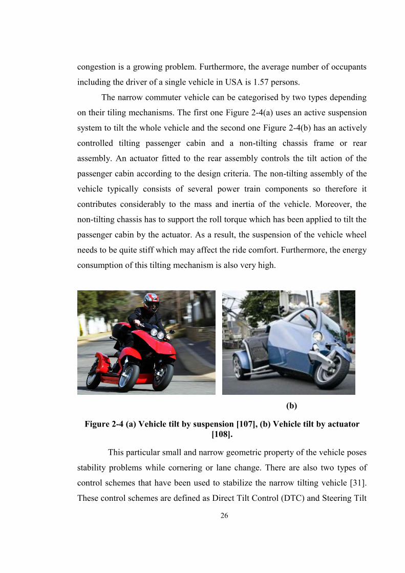
26
congestion is a growing problem. Furthermore, the average number of occupants
including the driver of a single vehicle in USA is 1.57 persons.
The narrow commuter vehicle can be categorised by two types depending
on their tiling mechanisms. The first one Figure 2-4(a) uses an active suspension
system to tilt the whole vehicle and the second one Figure 2-4(b) has an actively
controlled tilting passenger cabin and a non-tilting chassis frame or rear
assembly. An actuator fitted to the rear assembly controls the tilt action of the
passenger cabin according to the design criteria. The non-tilting assembly of the
vehicle typically consists of several power train components so therefore it
contributes considerably to the mass and inertia of the vehicle. Moreover, the
non-tilting chassis has to support the roll torque which has been applied to tilt the
passenger cabin by the actuator. As a result, the suspension of the vehicle wheel
needs to be quite stiff which may affect the ride comfort. Furthermore, the energy
consumption of this tilting mechanism is also very high.
(b)
Figure 2-4 (a) Vehicle tilt by suspension [107], (b) Vehicle tilt by actuator [108].
This particular small and narrow geometric property of the vehicle poses
stability problems while cornering or lane change. There are also two types of
control schemes that have been used to stabilize the narrow tilting vehicle [31].
These control schemes are defined as Direct Tilt Control (DTC) and Steering Tilt

27
Control (STC) systems as detailed in [27, 32, 109]. In the DTC system, the driver
steering input is connected to the front wheel steering mechanism directly [31].
In a DTC system, dedicated actuators control the tilt of the vehicle (such as
having an active suspension). In this system, the link between the wheels and the
steering wheel is no longer mechanical. In an STC system, on the other hand,
STC or steering tilt control, no additional actuator is used, and the tilt of the
vehicle is controlled by the steering angle input from the driver. The steering
input is used to follow the desired trajectory as well as stabilize the tilt mode of
the vehicle. This is particularly a steer-by-wire system [31]. In this system, the
driver steering input signal is read by the controller and the controller determines
the tilt angle. Since the beginning of the 1950s extensive research has been done
on both types of control systems by the automotive industry and researchers.
Motorised tilting vehicles have been studied and developed since the
pioneering prototype proposed by Ernst Neumann [22][43] in 1945–1950. The
Ford Motor Company developed a two-wheeled lean vehicle in the middle of the
1950s [43]. It was gyroscopically stabilised with retractable wheel pods for
parking [43]. In the 1960s, the MIT presented a tilting vehicle which was
equipped with an active roll control [43]. The design was similar to a motorcycle.
At the beginning of the 1970s, General Motors developed a tilting vehicle called
the ‘Lean Machine’. It had a fixed rear frame and a tilting body module that was
controlled by the rider. The rider had to balance the tilting body using foot pedals
[43] [27].
More recently, Brink Dynamics [25] developed a three wheeled car named
Carver with a rotating body and non-tilting rear engine. BMW and the
Universities of Bath and Berlin were presented Clever in 2003 [110]. It consists
of a non-tilting two-wheel rear axle and a single front wheel that tilts with the
main body. The rear body remains in contact with the ground in the same way as

28
a conventional automobile rear axle but the main body is connected to the rear
frame by a suspension layout enabling it to lean like a motorcycle.
The manufacturer Lumeneo presented the Smera and Piaggio presented
MP3 [111]. At the Tokyo motor show 2009 Nissan revealed the Land Glider
[22], which is a four wheeled narrow vehicle. Of all the above the Carver One
was sold commercially between 2006 to mid-2009 and the MP3 has been on the
market for sale since 2006 [43].
From an academic point of view researchers have done an extensive
amount of work on these cars. D. Karnopp suggested that the narrow tilting
vehicle would have to lean into a corner and also explained the optimum desired
lean angle in his research [26]. Dean Karnopp and his co-workers have also
carried out a significant amount of research into dynamic modelling of tilting
vehicles [31]. Karnopp and Hibbard have proposed that a tilt actuator can be
employed to tilt a narrow tilting vehicle to a certain desired tilt angle with the
help of the direct tilt control strategy [31]. It is apparent that their research lays
down the basic ideas for designing a direct tilt control system. However in some
of their research [26-28], they are unable to take into account the lateral position
acceleration of the vehicle while calculating the desired tilt angle calculation.
This caused the controller to require a high transient torque.
There are a few publications which have presented the idea of a virtual
driver in a narrow tilting vehicle. These virtual drivers are able to follow a path
without falling to one side. Saccon et al. [29] developed a dynamic inversion of a
simplified motorcycle model. This model is able to obtain a stabilizing feedback
through the standard Linear Quadratic Regulatory control system. This model
allows the controller to calculate the state and input trajectories according to a
desired output trajectory of the tilting vehicle. To avoid the direct deal with the

29
lean instability, Frezza and Beghi [30] took the roll angle as control input instead
of the steering angle input from the driver. They have defined the path tracking
as an optimization problem of the controller design.
Snell [112] proposed to start the tilting action with the STC system then to
switch to the DTC system to maintain the tilting position. A three wheeled
prototype of a narrow tilting vehicle was developed at the University Of Bath,
UK. It employed hydraulic actuators to tilt the cabin with the help of DTC
technology which has a high power requirement [113]. Kidane et al. [114],
applied hybrid control schemes with both STC and DTC. This work employed a
feed forward plus PID controllers to stabilize the tilt of the vehicle and a look-
ahead error of the trajectory model was used as the driver model. Chiou proposed
a double loop PID to control and to maintain the tilting position and the rate of
the vehicle [115].
Defoort [116] and Nenner et al., [117] worked with the trajectory-tracking
and robust stabilization problems of a rider-less bicycle. They developed a
dynamic model that considers geometric-stabilization mechanisms. They also
derived a combined control system consisting of a second-order sliding mode
controller and disturbance observer. In their research they adopted a simplified
tricycle model as the dynamic model of a bicycle .
In addition, in the research works stated above and in other authors’
researches, the effect of road bank angle is not considered in the control system
design and in the modelling of the dynamic model of narrow tilting vehicles [26,
27, 32, 36-44]. The result of not incorporating road bank angle is a non-zero
steady state torque requirement. It also significantly increases transient torque
requirements. Sang-Gyun So and D. Karnopp [28] considered the road bank
angle in their work, but it has no effect on the final form of the control input [31].

30
The authors specified that the lateral acceleration of the vehicle be obtained from
the sensor readings mounted on the vehicle. But it is evident that the reading of
an accelerometer of a narrow tilting vehicle would be contaminated by the tilt
angle, the road bank angle and the angular acceleration of the vehicle [31].
2.3.2 Tilting standard production vehicle
To improve vehicle performance during cornering or sudden lane change
advance electromechanical and electronic systems are used, for example, antilock
braking systems, electronic brake force distribution, active steering and
electronic stability programs. Nowadays, some researchers have focused on
active steering control to improve vehicle cornering [17-19]. Recently, a system
was presented by Bose Corporation, namely, the Bose suspension system [34].
This system consists of a power amplifier and a linear electromagnetic motor at
each wheel that is controlled by a set of control algorithms. The high-bandwidth
linear electromagnetic dampers of this system respond quickly enough to achieve
better ride performance. To date the prototype of the Bose suspension system is
installed in standard production vehicles and able to achieve superior comfort
and control simultaneously. According to the manufacturer, the Bose suspension
system can counter the body roll of the vehicle by stiffening the suspension while
cornering. It can also change the ride height dynamically and is capable of
performing the four quadrant operations and the high bandwidth operation. But it
uses less than one third of the power of the air conditioning system of a typical
vehicle. However, to date no commercial tests or design details are available to
the world from the Bose Corporation which would allow an accurate and
unbiased comparison with other competitive suspension systems.
Vehicle performance during cornering has been improved by most car
manufacturers using electronic stability control (ESC). Car manufacturers use
different brand names for ESC, such as Volvo call it DSTC (Dynamic Stability
and Traction Control); Mercedes and Holden call it ESP (Electronic Stability

31
Program); DSC (Dynamic Stability Control) is the term used by BMW and
Jaguar but whatever the term used the processes are almost same. To avoid over
steering and under steering during cornering, ESC extends the brake and
different torque on each wheel of the vehicle. But ESC reduces the longevity of
the tyre because the tyre skids during random braking. To overcome this problem
a vehicle can be tilted inwards via an active or semi-active suspension system.
Figure 2-5 Nissan Land Glider [35].
Car giant Nissan has developed a four wheeled ground vehicle for the
future which is half-scooter and half-car [35]. The electric-powered Land Glider
shown at Figure 2-6 is approximately half the width of a family car and is
designed for busy city streets. It uses a steer-by-wire system to control the
vehicle manoeuvrer and has small motors mounted at each wheel. A computer in
the Land Glider automatically calculates the amount of lean required to corner
considering the speed, steering angle and yaw rate of the vehicle. The vehicle
body can lean into a corner up to 17 degrees for sharper handling. In addition, in
the works stated above and other authors’ researches, the effect of road bank
angle is considered neither in the control system design nor in the modelling of
the dynamic model of the tilting vehicles.

32
2.4 Conclusion
For a long time, active and semi-active suspension systems have been employed
as a practical application for modern control theory. In this literature review
many robust and optimal control approaches or algorithms have been reviewed
including linear time invariant H-infinity control (LTIH), linear parameter
varying control (LPV) and model-predictive controls (MPC). Five widely known
control approaches are reviewed more deeply, namely the Linear quadratic
regulator & Linear Quadratic Gaussian, sliding mode control, Fuzzy and neuro-
fuzzy control and the sky-hook and ground-hook approaches. It has been found
that the skyhook control strategy is the most widely used due to its simplicity for
practical implementation. But still, there is a great scope of work yet to be done
to modify the skyhook control strategy to achieve better performance. Different
types of damper technologies have also been discussed in this chapter and it has
been shown that the linear electromagnetic damper is best for the semi-active
suspension system due to its fast response time which is better than the best
hydraulic device. A brief literature review on automotive tilting technology has
also been done in this chapter. This highlights that a direct tilting method needs
to be developed to tilt the standard passenger vehicle inward during cornering
while considering the road bank angle.

33
Chapter 3 Vehicle suspension system
3.1 Overview
The quarter-car suspension model is the best bench-mark to study and analyse
the dynamic behaviour of vehicle vertical isolation properties. This chapter
presents background information and a description of the quarter-car suspension
model which includes passive, semi-active and active suspension. This chapter
also consists of a comparison of various models to determine the appropriate
quarter-car model to compare the control systems discussed in Chapter 4.
3.2 Vehicle suspension system
Figure 3-1 Suspension system [118].
A suspension system is an essential element of a vehicle to isolate the frame of
the vehicle from road disturbances. Figure 3-1 shown here is a typical car
suspension system. It is required to maintain continuous contact between a

34
vehicle’s tyres and the road. The most important element of a suspension system
is the damper. It reduces the consequences of an unexpected bump on the road
by smoothing out the shock. In most shock absorbers, vibration energy is
converted to heat and dissipates into the environment. Such as, in the viscous
damper, energy is converted to heat via viscous fluid. In hydraulic cylinders, the
hydraulic fluid is heated up. In air cylinders, the hot air is emitted into the
atmosphere. But the electromagnetic damper is different; here the vibration
energy is converted into electricity via an electric motor (induction machine or
DC motor or synchronous machine) and stored in a condenser or battery for
further use [119].
Suspension systems are categorized as passive, active and semi-active
considering their level of controllability. Although all the types of the suspension
systems have different advantages and disadvantages, all of them utilize the
spring and damper units.
3.2.1 Passive suspension system
Figure 3-2 Passive suspension system.

35
Passive suspension systems are composed of conventional springs and oil
dampers with constant damping properties (Figure 3-2). .In this model m1 and m2
represent the un-sprung mass and sprung mass respectively, k 1 is the tyre
stiffness coefficient or tyre spring constant, k 2 is the suspension stiffness or
suspension spring constant. c0 and ct are the suspension damping constant and
the tyre damping constant respectively, Fr is friction of suspension, q, z1,
z2 represents road profile input, displacement of un-sprung mass
and displacement of sprung mass respectively
In most instances, passive suspension systems are less complex, more
reliable and less costly compared to active or semi-active suspension systems.
The constant damping characteristic is the main disadvantage of passive
suspension systems. For a passive suspension, the use of soft springs and
moderate to low damping rates is needed but the use of stiff springs and high
damping rates is needed to reduce the effects of dynamic forces. Designers utilize
soft springs and a damper with low damping rates for applications that need a
smooth and comfortable ride such as in a luxury automobile.
On the other hand, sports cars incorporate stiff springs and a damper with
high damping rates to gain greater stability and control at the expense of comfort.
Therefore, the performance in each area is limited for the two opposing goals
[120]. There is always a compensation need to be made between ride comfort and
ride handling in the passive suspension system as spring and damper
characteristics cannot be changed according to the road profile.

36
3.2.2 Semi-active suspension System
Figure 3-3 Semi-active suspension system.
The semi-active suspension system was first proposed by Karnopp et al. in
1973 [52].In this model, Figure 3-3 is a semi-active suspension model. Here fd
can generate an active actuating force by an intelligent controller. Since then,
semi-active suspension systems have continued to acquire popularity in vehicular
suspension system applications, due to their better performance and
advantageous characteristics over passive suspension systems. In semi-active
suspension systems, the damping properties of the damper can be changed to
some extent. The adjustable damping characteristics in semi-active dampers are
achieved through a variety of technologies, such as: Electro-Rheological (ER)
and Magneto-Rheological (MR) fluids, solenoid-valves and piezoelectric
actuators. It has been widely recognized that a semi-active suspension system
provides better performance than a passive system. As it is safe, economical and
does not need a large power supply, semi-active suspension has recently been
commercialized for use in high-performance automobiles [121-125]. However,
there still exist many challenges that have to be overcome for these technologies
to achieve their full potential. MR degradation with time, sealing problems and
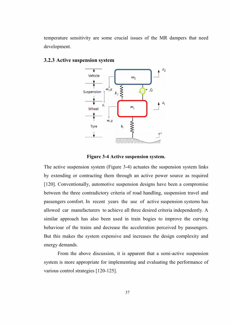
37
temperature sensitivity are some crucial issues of the MR dampers that need
development.
3.2.3 Active suspension system
Figure 3-4 Active suspension system.
The active suspension system (Figure 3-4) actuates the suspension system links
by extending or contracting them through an active power source as required
[120]. Conventionally, automotive suspension designs have been a compromise
between the three contradictory criteria of road handling, suspension travel and
passengers comfort. In recent years the use of active suspension systems has
allowed car manufacturers to achieve all three desired criteria independently. A
similar approach has also been used in train bogies to improve the curving
behaviour of the trains and decrease the acceleration perceived by passengers.
But this makes the system expensive and increases the design complexity and
energy demands.
From the above discussion, it is apparent that a semi-active suspension
system is more appropriate for implementing and evaluating the performance of
various control strategies [120-125].

38
3.3 Quarter-car suspension model
In this research, a two degree of freedom quarter-car model has been used to
evaluate the performance of various controllers as described in Chapter 4. A
quarter-car model imitates the heave or the vertical motion of the vehicle alone.
As the design goal of most semi-active suspension system is to reduce the
vertical acceleration, the quarter-car model is sufficient for evaluating the
performance of control strategies [53]. The sprung mass, suspension components,
un-sprung mass and a wheel are the basic components of a quarter-car model.
For a quarter-car model, sprung mass means the body or chassis of the car and it
represents almost one fourth of the weight of the whole body of the car. The
suspension system bridges the connection between the wheel and body of the car
and consists of many parts, and varies according to the type of the suspension
system such as passive, semi-active or active suspension (described in the
previous section). Un-sprung mass includes the weight of everything
geometrically below the suspension system, such as axle, wheel and rim. The
wheel denotes the tyre, which incorporates the spring and damping
characteristics.
Figure 3-5 (a) Ideal quarter-car model, (b) simplified quarter-car model.

39
A two degree of freedom quarter-car model as shown in Figure 3-5(a) is
known as an ideal model and used by some researchers [126-128]. Faheem et al.,
[129] presented an insight on the suspension dynamics of the quarter car model
with a complete state space realisation. In the ideal case the sprung mass and un-
sprung mass is free only to bounce vertically. In this model m1 and m2 represent
the un-sprung mass and sprung mass respectively, k 1 is the tyre stiffness
coefficient or tyre spring constant, k 2 is the suspension stiffness or suspension
spring constant. fd can generate an active actuating force by an intelligent
controller. c0 and ct are the suspension damping constant and the tyre damping
constant respectively, Fr is friction of suspension, q, z1, z2 represents road profile
input, displacement of un-sprung mass and displacement of sprung mass
respectively. The ideal dynamic equations of motion of un-sprung and sprung
masses which satisfy Newton’s second law of motion are given by the equation
3.1.
gmFfzzkzzczm
gmFfqzkqzczzkzzczm
rd
rdt
2202
11201
12122
1121211
(3.1)
The simplified model as shown in (b) has been used in most recent studies
[16, 130-133] as the effect of the tyre damping coefficient ct is negligible
compared to the tyre stiffness coefficient. So omitting the tyre damping force ct
(
qz2 ), the equation (3.1) becomes
gmFfzzkzzczm
gmFfqzkzzkzzczm
rd
rd
2202
11201
12122
121211
(3.2)
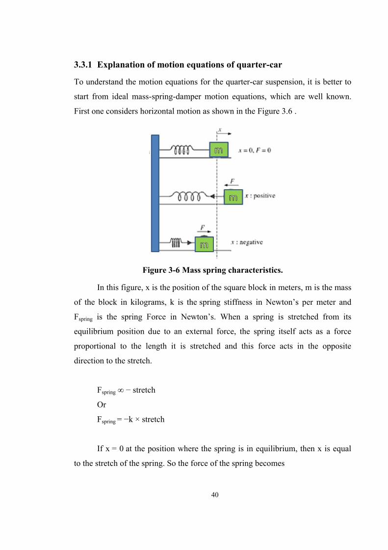
40
3.3.1 Explanation of motion equations of quarter-car
To understand the motion equations for the quarter-car suspension, it is better to
start from ideal mass-spring-damper motion equations, which are well known.
First one considers horizontal motion as shown in the Figure 3.6 .
Figure 3-6 Mass spring characteristics.
In this figure, x is the position of the square block in meters, m is the mass
of the block in kilograms, k is the spring stiffness in Newton’s per meter and
Fspring is the spring Force in Newton’s. When a spring is stretched from its
equilibrium position due to an external force, the spring itself acts as a force
proportional to the length it is stretched and this force acts in the opposite
direction to the stretch.
Fspring ∞ − stretch
Or
Fspring = −k × stretch
If x = 0 at the position where the spring is in equilibrium, then x is equal
to the stretch of the spring. So the force of the spring becomes

41
Fspring = − k x
In addition, there is a force that opposes the motion of the mass as shown
in the Figure 3-7.
Figure 3-7 Mass-spring-damper configuration.
In this figure, c is the damping constant in Newton-second per meter and v
is the velocity of the block in meters per second. This force is the damping force
and it is proportional to the mass velocity which also opposes the mass velocity,
such as
Fdamping ∞ − v
Or
Fdamping = −c v
So the total force acting on spring-mass-damping system is
F = Fspring + Fdamping = − k x − c v
According to Newton's law of motion F = m a. From the definition of
acceleration, the first derivative of position x is equal to the velocity v and the
acceleration a is equal to the second derivative of position x. so

42
xa
And
xv
Now the differential equation becomes,
xkxcxm
(3.3)
The simple mass-spring-damper model described above is the foundation
of vibration analysis. This is defined as the single degree of freedom (SDOF)
model, since it has been assumed that the mass only moves up and down in the
same axis. The Figure 3-8 is a more complex system involving more mass which
is free to move in more than one direction – adding degrees of freedom.
Figure 3-8 Two degree of freedom horizontal multiple mass spring damper.
In this model, the two springs act independently, so it is easy to figure out
the forces acting on the two blocks. It is assumed that the connection of the
spring and damper to the wall is the origin of this suspended system. Here
x1, x2 are the position (left edge) of the blocks, m1, m2 are the mass of blocks and
k1, k2 are the spring constants. So the motion equations would be
xkxxkxcxxcxm 112121 211211
xxkxxcxm 12122 222
(3.4)

43
Figure 3-9 Vertical multiple mass spring damper configuration.
Now the vertical linear motion has been considered as showed in the
above figure. Here a new force strikes due to gravitation g (m/s2) which acts in
the same direction (downward) as the mass velocity and equals the product of
mass and gravity, so the differential equation becomes
gmxkxxkxcxxcxm 1112121 211211
2 2 1 2 12 2 2 2gm c k mx x x x x
(3.5)
Now, considering a two degree of freedom quarter-car suspension model
having an actuator which delivers a force fd as shown in the (a) and the
corresponding motion equation is the equation (3.1).
Figure 3-10 Forces acting at a point.

44
If one considers the forces acting on the un-sprung mass m 1 then the
forces acting downward is the m1g force due to gravitation and actuating force fd.
According to Figure 3-10 force due to the acceleration of the un-sprung mass
zm 11
is acting in the upward direction. If the displacement z1>q is positive then
the spring force k1(z1-q) and the damping force c1(z1-q) is negative in the
downward direction according to (a). This is same for a damping force of co and
a spring force of k2 if z1>z2 is positive. The friction force Fr is acting negatively
in the downward direction.
Again for sprung mass m2, the forces acting downward is the m1g force
due to gravity and friction force Fr. The force due to the acceleration of the
sprung mass zm 22
is acting in the upward direction. The actuating force fd is
acting negatively downward. Damping force of co and spring force of k2 is
negative in the downward direction under the condition that displacement z2>z1.
3.3.2 High vs. low-bandwidth suspension system
A semi-active suspension system has two sections: semi-active and passive. The
semi-active part usually gets damping force from an external energy source to
control the suspension system (in regenerative type system, it may differ). The
passive part has a spring and a damper or similar devices. In some systems this
part is rigid but it can be omitted as well. This can be distinguished as low-
bandwidth and high-bandwidth suspension systems [134].

45
(a) (b)
Figure 3-11 (a) Low-bandwidth suspension model, (b) high-bandwidth suspension model.
Low-bandwidth configuration (LBC) represents the series connection between
the active and passive components of the suspension system (Figure 3-11 (a)). In
the mathematical modelling, the differential motion equations are as follows,
gmFzzkzzczm
gmFqzkzzkzzczm
rlblb
rlblb
2222022
111222011
1
(3.6)
where c(dzlb – dz1) = fd is the actuating force. Through LBC
configuration, the active suspension system can control the car body (sprung
mass) height. But the actuator cannot be omitted or turned off as it carries the
static load. Another disadvantage of this system is that it is good only in the low
frequency range.
On the other hand, in a high-bandwidth configuration (HBC), it is possible
to control at higher frequencies than for LBC and also the passive part can work
alone in case of failure of the active part. The only drawback of HBC is that
practically it can’t control the vehicle height. In a HBC configuration, active and

46
passive components are linked in parallel (Figure 3-11(b)). The motion equations
of HBC are almost similar to that of LBC but an extra term is added which is an
actuator force fd.
In this research, a two degree of freedom HBC semi-active suspension
system is used, mainly because there is no requirement of a static load force.
3.4 Comparison of recent models
Comparison between different quarter-car suspension systems described in the
literature has been done considering the quarter-car model travelling over a ramp
in the street as shown in Figure 3-12 This is the road profile input q for the
quarter-car suspension model.
Figure 3-12 The road profile.
The quarter-car suspension model used in this comparison analysis has
been shown in (b). The parameters of quarter-car models chosen by different
authors in their recent research have been extracted and described in the table
below.

47
Table 3-1 The parameters of quarter-car models.
Model
No.
Model
Authors’
m 1
kg
m 2
kg
k 1
N/m
k 2
N/m
c 0
N-s/m
1 Yi Chen 2009 [1] 36 240 160000 16000 1400
2 Hongkun Zhang et al.
2009 [126] 31 380 228000 29000 1500
3 Jia-ling and Jia-qiang
et al. 2006 [135] 20 160 100000 10000 2000
4 Nguyen and Choi 2009
[51] 31 230 130000 16000 1400
5 Scheibe and Smith
2009 [133] 35 250 150000 29000 1400
6 Gopala Rao and
Narayanan 2009 [136] 1009 1000 360000 36000 1000
7 Priyandoko, Mailah et
al. 2009 [132] 25 180 190000 16000 1000
8 Fateh and Alavi 2009
[128] 40 243 124660 14671 370
9 Gao, Zhang et al. 2008
[2] 36 240 160000 16000 980
10 Du, Zhang et al. 2008
[137] 40 320 200000 18000 1000
11 Sung, Han et al. 2008
[138] 40 380 309511 28516 1284
The above stated models have been simulated in the MatLab/Simulink
environment and the sprung mass acceleration of quarter-car models of different
authors have been shown in the figures below

48
(a)
(b)
Figure 3-13 (a) Comparison between passive suspension models 1 to 6, (b) Comparison between passive suspension models 1 and 7 to 11.

49
As the negative amplitudes are almost the opposite mirror of the positive
ones these are not shown in figure above.
Figure 3-13 shows the comparison between different authors quarter-car
models based on their chosen parameters m1, m2, k1, k2 and c2 as stated in Table
3-1. In this comparison peak amplitude and settling time of sprung mass
acceleration has been considered.
According to Table 3-2, the model used by Hongkun Zhang et al. (2009)
[126] has a peak amplitude reduced by 17% from Yi Chen’s (2009) [1] model
whereas the settling time increases by 23%. Again, in a comparison with Yi
Chen’s (2009) [1] model, the model used by Priyandoko, Mailah et al. (2009)
[132] has a settling time that decreases by 5% but peak amplitude increases by
6%.
Furthermore the overall performance of Yi Chen’s (2009) [1] model is the
best compromise compared to other models in terms of peak amplitude and
settling time.

50
Table 3-2 Comparison between outputs of the vehicle sprung mass acceleration.
Model
No.
Model
Authors
Maximum
positive
amplitude (m/s2 )
Settling time
( s )
1 Yi Chen 2009 [1] 8.69 2.87
2 Hongkun Zhang et al. 2009
[126] 7.24 3.53
3 Jia-ling and Jia-qiang et al.
2006 [135] 11.31 2.33
4 Nguyen and Choi 2009 [51] 8.47 2.98
5 Scheibe and Smith 2009 [133] 9.31 2.97
6 Gopala Rao and Narayanan
2009 [136] 5.77 12.4
7 Priyandoko, Mailah et al.
2009 [132] 9.23 2.72
8 Fateh and Alavi 2009 [128] 7.11 11.4
9 Gao, Zhang et al. 2008 [2] 7.49 3.65
10 Du, Zhang et al. 2008 [137] 6.61 4.12
11 Sung, Han et al. 2008 [138] 7.46 3.33

51
3.5 Conclusions
In this chapter, the vehicle suspension system has been categorised and discussed
briefly. It has been explained that the semi-active suspension system is the most
suitable for investigation in this research. A brief description of the quarter-car
model has been given as well as an explanation of the motion equations used in
the model. High and low bandwidth suspension systems have also been
discussed. As there is no requirement of a static load force in this research, in
Chapter 4 a two degree of freedom HBC semi-active suspension system is used
to investigate different semi-active control algorithms. An extensive comparison
of quarter-car models extracted from the study of various researchers has been
presented in this chapter. From the comparison, it has been concluded that the
better estimation of the parameters of mass, spring constant and damping
coefficient for a passive quarter-car model is Yi Chen’s (2009) [1] model and this
model has been used for further investigation. The semi-active control algorithms
experiments are discussed in the next chapter.

52
Chapter 4 Design of semi-active suspension system
4.1 Overview
One of the key issues in the design of an active or semi-active suspension system
is to identify the appropriate control algorithm. This chapter describes the
proposed modified skyhook control closed loop feedback system and its
effectiveness in a semi-active suspension system. The chapter comprises four
main sections. The first section describes the proposed and three existing
skyhook control algorithms while the second section describes the road profile
that needs to be generated to evaluate the controller performances. The third
section presents the simulation of the quarter-car model as described in Chapter 3
with the semi-active control algorithms. The last section is comprised of
simulation and experimental analysis of the Quanser quarter-car suspension plant
designed and manufactured by Quanser Inc. The last two sections also compare
the results of different control techniques and evaluate the proposed modified
skyhook control algorithm. Comparison has been done in terms of ride comfort
and road handling performance. On the other hand, the evaluation consists of a
human vibration perception test and admissible acceleration levels test based on
ISO 2631.
4.2 Semi-active control algorithms
On the basis of the two degree of freedom semi-active suspension system
described in Chapter 3, a passive and four semi-active suspension systems have
been modelled. The continuous skyhook control of Karnopp et al. [14], modified
skyhook control of Bessinger et al. [15], optimal skyhook control of Nguyen et
al. [51], and the proposed modified skyhook control strategies used in designing
the semi-active suspension system. The control strategies are described below.

53
4.2.1 Continuous skyhook control of Karnopp et al. (1974)
The semi-active continuous skyhook control strategy of Karnopp et al. [14] can
be represented by the following equation.
(4.1)
Where fd is the semi-active damping force of the actuator. This strategy is
used in many recent studies [139] [140]. According to this control strategy, the
effective damping of the skyhook damper is bounded by a high and a low level.
Determining, whether the damper is to be adjusted to either its low state or its
high state depends on the product of the velocity of the spring mass attached to
that damper
2z and the relative velocity across the suspension damper
12 zz . If
this product is greater than or equal to zero, then the high state of the damper is
applied. If this product is negative, the damper is adjusted to its low state. In this
situation, it is better to supply no force at all but in practice the semi-active
damper coefficient is limited by the physical parameters of the conventional
damper, which means that there is both an upper bound, Cmax; and a lower bound,
Cmin and they have certain values depending on the chosen damper. Here Csky is
the nominal damping coefficient selected by the designer and Cmax < Csky < Cmin.
4.2.2 Modified skyhook control of Bessinger et al. (1995)
The modified skyhook control strategy presented by Bessinger et al. [15] is a
modification of the original skyhook control strategy proposed by Karnopp et al.
in 1974 [14]. Bakar et al., [97] have also used the same strategy in their research.
Both the passive damper and skyhook damper effects are included in the

54
modified skyhook control algorithm to overcome the problem caused by the
application of the original skyhook controller known as the water hammer [98]
[99]. The water hammer problem is one where the passenger experiences
unwanted harsh jerks and audible noise created by the force discontinuity (caused
by low damping switches to high damping or vice versa). The equation of the
modified skyhook control algorithm is given by
sky ( )2 1 2d 1f C z z z
(4.2)
Where α is the passive to skyhook ratio and Csky is the damping constant
of a modified skyhook control. The value of α is chosen to be 0.5 and an optimal
value of Csky is chosen such that the desired force estimated from this control
algorithm is to be within the range of damping forces of the designed damper.
4.2.3 Optimal skyhook control of Nguyen et al. (2009)
Nguyen et al. [51] have described the semi-active optimal skyhook control
strategy by the following equation.
(4.3)
Where factual = fd is the semi-active damping force of the actuator, fmax =
Cmax × (
12 zz ) and fmin = Cmin × (
12 zz ) are the maximum and minimum
damping forces that can be exerted by the actual damper at a given relative
velocity, respectively. u = Csky ×
2z is the damping force exerted by the damper

55
where Csky is the optimal damping coefficient obtained by the following equation
in the simulation environment.
sky OptimalRMSmin JC
(4.4)
Where 2 1 32 11 2 qz z ww wz zJ
RMSRMS
(4.5)
Here wi, i =1, 2, 3 are the set values of weighting factors according to the
defined objective which is minimizing the criterion of Csky (optimal).
4.2.4 Proposed skyhook control with adaptive skyhook gain
The proposed modified skyhook control algorithm is chosen to provide the
desired force in attenuating road harshness in the real world. From the discussion
in the literature review and Sections 4.2.1, 4.2.2, 4.2.3, it has been understood
that the designers have chosen or derived (trial and error methodology) a constant
value of Csky for their skyhook control strategy and used the same value for all
road conditions. In the real world, a vehicle is not always travelling on the same
type of road and it is very difficult to imitate all types of road surfaces in a
simulation environment. The road disturbance interacting with the vehicle tyre in
the real world is quite different compared to the road disturbance modelled in the
simulation environment. A good semi-active suspension system should provide
high damping on good roads for better body isolation, low damping on average
roads to achieve good comfort and finally, adequate damping on the poor roads
for structural modes (Road profile description is given in Section 4.3). Skyhook
gain should be varied according to the road surface on which the vehicle is
travelling. The proposed modified skyhook control strategy with adaptive gain
(illustrated in Figure 4-1) is developed to address this problem. A modification of
conventional continuous skyhook control has been proposed and it is described
by equation (4.6).

56
(4.6)
Cmax and Cmin represent the maximum and minimum damping coefficient
of the actuator respectively. The value of Csky is varied in accordance with the
road profile input. The velocity of the sprung mass relative to the un-sprung mass
(
12 zz ) is denoted as positive when the base and mass of the suspension system
are splitting (i.e., when z2 > z1). If in (b), the sprung and un-sprung masses are
splitting, the semi-active damper becomes in tension. As a result, the force fd
works in the negative z2 direction which is applied to the sprung mass by the
actuator. In the following equation, fd is pointing in the opposite direction of z2.
fd = − C0 ×
2z (4.7)
where C0 is the required damping coefficient of the actuator. Since the
actuator is capable of producing a force in the appropriate direction, the only
requirement to match the skyhook suspension is:
sky
1 2
0
2
z zC C
z
(4.8)
This control strategy dictates the actuator movement and also determines
the specific value of Csky for the road surface on which the vehicle is travelling.
At first the road profile input is captured by the tyre deflection
measurement over a certain period of time while the vehicle is travelling on the
road. Then the quarter-car model identical to 1/4th of the vehicle suspension

57
system is simulated in the simulation environment (on-board system placed in the
vehicle) as both uncontrolled (Passive) and controlled (Semi-active) suspension
system. The controlled suspension system is dictated by the modified skyhook
control strategy described in equation (4.6) with a range of Csky (The range is
depicted by the rated maximum and minimum damping coefficient of the
actuator). The RMS values of sprung mass acceleration of both controlled and
uncontrolled suspension systems are calculated and a performance index (PI) is
derived by the following equation described by Sung et al. [138].
,
,
PI
N 22 Ci 1
N 22 UCi 1
iz
iz
(4.9)
Then the optimal value of Csky is chosen for which the PI becomes
minimum,
sky OptimalPIminC (4.10)
This optimal value of Csky replaces the initial value of the skyhook gain of
the modified skyhook controller which is dictating 1/4th of the vehicle
suspension system for the next certain period of time. This time interval would
be determined by the processor speed of the onboard computer of a vehicle.
While Csky is calculated the suspension system behaves according to the modified
skyhook control law with an initial or previous value of Csky. After each certain
period of time interval Csky is adapted according to the road surface to achieve
better performance. The whole process is represented in the Figure 4-1.

58
Figure 4-1 Schematic of the suspension systems based on proposed modified
skyhook control system with adaptive skyhook gain.
To investigate how the controller behaves under different road conditions,
a road profile needs to be generated. The next section describes the road profile.

59
4.3 Road profile description
In order to validate the quarter-car model and its parameter estimation, one needs
to run the simulation of the model on a road surface which is adopted by most
researchers. To predict the response of quarter-car models it is often beneficial to
handle the excitation created by road irregularities as the spectrum of a
geometrical road profile, P(n) [141]. This can be expressed as
(4.11)
Where P (n0) is the road roughness, n is a spatial frequency, n0=1/2π c/m,
and w1 = 2.0 and w2 = 1.5. The drop in magnitude is modelled by the waviness ω.
ISO standards suggest ω = 2 for road undulations [142]. In this study, three
classes of roads are used as defined by ISO8608 [50] and there P(n0) values are
given in Table 4-1.
Table 4-1 Theoretical road classes on basis of road roughness.
Road Class Road roughness P(n0) (m3/c)
A (Good) 16×10-6
B (Average) 64×10-6
C (Poor) 256×0-6

60
The road irregularity also depends on vehicle speed. If a vehicle is
travelling on L length of road segment with speed V then the road profile is
described by a superposition of N → ∞ sine waves:
sinRP( )N
i iii 1
tt A
(4.12)
Where Ai=√(2p (Ωi) 2π/L), i = 1, 2, 3, N, αi is a random variable with a
uniform distribution in the interval [0, 2 π] [43]. The value of Ω is determined by
VL2
(4.13)
It has been assumed that vehicle speed V = 20 m/s, the distance travelled
by the vehicle L =200 m and time taken t = 10 s. Super position of N = 100 has
been chosen in this analysis as the standard of ISO8606. Figure 4-2 (a) and (b)
describe the time histories and power spectral density of three classes of roads
respectively.

61
(a)
(b)
Figure 4-2 (a) The time histories of three classes of roads, (b) Power spectral density of three classes of road.

62
4.4 Comparison and evaluation using Y. Chens’ model
The parameters of the two degree of freedom of Y. Chen’s [1] quarter-car model
used in Chapter 3 are listed in the following table.
Table 4-2 Nominal parameter values used in simulation.
Parameter Definition Values
m1 un-sprung mass 240 [kg]
m2 sprung mass 36 [kg]
k1 tyre spring coefficient 160000 [N/m]
k2 suspension spring coefficient 16000 [N/m]
c0 suspension damping coefficient 1400 [N-s/m]
Fr friction of suspension 300 [N]
g Gravity acceleration 9.8 [m/s2]
To investigate how the controller behaves under different road conditions
a road profile is generated using the three classes (A, B and C) of road profiles
where each class lasts for 20s. The Figure 4-3 shows the road profile input that
has been used in the simulations to compare the performance of the controllers.

63
Figure 4-3 The time history of road profile.
The reaction of the road profile input shown by the passive and four semi-
active suspension systems described above is depicted in Figure 4-4. Random 5s
along the total length of the simulation is shown for better visualization.
Figure 4-4 The sprung mass acceleration of the passive and semi-active
suspension systems.
The comparison of the results is discussed in the next sub-sections.

64
4.4.1 Comparison
To compare, the controllers’ performances, ride comfort and road handling
performance is calculated in the following section.
4.4.1.1 Comparison on ride comfort performance
Ride comfort depends on human perceptions of vehicle noise, vibration and
motion. While it varies from person to person, a quantitative evaluation of the
ride comfort performance (RCP) can be carried out following the methodology
provided by Abramov et al. [142] and that is, the root mean square of the sprung
mass acceleration normalized by the gravity acceleration g,
/
dNRMS
1 22T
2
t 0
t1 z tT g
(4.14)
Here T is the duration of exposure. Lower NRMS value represents higher
passenger comfort [142]. The NRMS achieved in simulation and experiment by
the passive and four semi-active suspension systems are shown in the Figure 4-5.

65
Figure 4-5 The ride comfort performance comparison.
The figure above shows the improvements on the comfort index (NRMS)
of the semi-active systems with respect to the passive suspension system. The
proposed modified skyhook control strategy; optimal skyhook control of Nguyen
et al. [51]; modified skyhook control of Bessinger et al. [15]; and continuous
skyhook control of Karnopp et al. [14] is improved by 38.4%, 27.3%, 2.8% and
5.9% respectively.
4.4.1.2 Comparison on road handling performance
To examine the ride handling performance of a vehicle, the forces acting on the
tyres and the road should be considered. The vehicle's reaction point with the
road disturbance is the tyres. For a quarter-car model, the force exchanged
between the road and tyre is Fz1 = k1 (z1 – q). Then the vehicle’s road handling
performance (RHP) can be calculated by the root mean square of the forces
normalized by the static forces which acts on the wheels. The static forces are
represented as (m1+m2)g [142],

66
/
dRHP )(
1 22T Z1
21t 0
t1 F tT m gm
(4.15)
Figure 4-6 The road handling performance comparison.
Higher RHP value represents higher ride handling performance
[142].Compared to the passive suspension system the figure above shows that the
RHP of the semi-active suspension system controlled by the proposed modified
skyhook control approach, optimal skyhook control of Nguyen et al. [51],
modified skyhook control of Bessinger et al. [15] and continuous skyhook
control of Karnopp et al. [14] decreases by 9.3%, 4.6%, 8.9% and 11.4%
respectively
4.4.2 Evaluation
The proposed modified skyhook controller performance is validated in terms of
the human vibration sensitivity test and the ride comfort level test specified by
the International Organization for Standardization ISO 2631 [143].

67
4.4.2.1 Human vibration sensitivity
The human vibration sensitivity test is more suited for a full car model instead of
a quarter-car model but if the quarter-car model is considered as a one wheel
vehicle or any instants, if the vehicle’s body vibration depends only on one wheel
then this sensitivity test can be run on a quarter-car model [134]. Study shows
that human beings are very sensitive to the vertical motion in the frequency range
of 4 to 8Hz [134]. So while designing a vehicle suspension, sprung mass
acceleration tolerance should be kept to a minimum keeping in mind the
frequency range mentioned above.
Figure 4-7 Vertical vibration of car suspension in frequency domain.
In the figure above, it is clearly shown that at low frequency, vertical
vibration of the sprung mass of the semi-active suspension system controlled by
the proposed algorithm remains almost zero for each class of road disturbance.
4.4.2.2 Admissible acceleration levels test based on ISO 2631
Ride comfort depends on human sensitivity to vehicle noise, vibration and
motion. It varies from person to person but a quantitative evaluation of the ride
comfort performance can be done following the methodology provided by ISO.

68
The international code ISO 2631 [143] defined a term named weighted RMS
acceleration (denoted here as WRMS) which can be formulated by the following
equation;
/
, dWRMS
1 22T N2 ii
i 1t 0
1 t tzFT
(4.16)
Where i= 1, 2, 3, N, T is the duration of exposure and Fi is the weighting
coefficients of acceleration in the vertical direction.
The WRMS value of the sprung mass obtained in this simulation is 0.71
for road class C. This confirms the validation of the proposed modified skyhook
control system in terms of ride comfort enhancement for a two degree of freedom
semi-active suspension system.
4.5 Comparison and evaluation of Quanser suspension plant
In this study a two degree of freedom Suspension plant provided by Quanser
[144] has been used to evaluate the controller’s performance. The description of
the plant is given below.
4.5.1 Quanser quarter-car suspension plant
The Quanser Suspension plant is a bench-scale model which imitates a two
degree of freedom quarter-car model dictated by a semi-active Suspension
system. Figure 4-8 shows the full model of the Quanser Suspension plant.

69
Figure 4-8 Quanser Suspension Plant.
As a nomenclature of the Quanser Suspension system, the table below
provides a list of all the principal elements combined in the equipment. On the
Quanser Suspension system represented in the figure above, each and every
element is located and identified through a unique identification (ID) number in
Figure 4-9.

70
Table 4-3 Nomenclature of Quanser Suspension System Components.
ID
# Description
ID
# Description
1 Top Plate (Blue, Vehicle Body Mass) 18 Lead Screw
2 Accelerometer Gain Potentiometer 19 Encoder Thread
3 Middle Plate
(Red, Vehicle Tyre Mass) 20 Stainless Steel Shafts
4 Suspension Encoder 21 Accelerometer
5 Bottom Plate (White, Road) 22 Accelerometer Connector
6 Suspension Motor Capstan Cable 23 Plant Top Cover
7 2 Adjustable Springs
(Vehicle Suspension Springs) 24 Limit Switch Safety Lights
8 Spring Holder Set Screw 25 Plant Handles
9 2 Adjustable Springs
(Vehicle Tyre Springs) 26 Bottom Plate Motor Connector
10 Linear Bearing Blocks 27 Limit Switch Push Key
11 Bottom Plate Encoder Connector 28 Safety Rod
12 Top Plate Encoder Connector 29 Movable Spring Holders
13 Bottom Plate Counter Weight Springs 30 Safety Limit Switch
14 Payload Mass (Brass) 31 Suspension Motor Connector
15 Quanser Suspension DC Motor 32 Suspension Encoder Connector
16 Bottom Plate Encoder 33 Encoder Thread Anchor
17 Bottom Plate Servo Motor 34 Top Plate Encoder

71
(a) (b)
(c)
(d) (e)
Figure 4-9 Quanser Suspension Plant: (a) Front Top Panel View, (b) Quanser Suspension System Side View, (c) Quanser Suspension Plant. Front
Bottom Panel View, (d) Quanser Suspension System Bottom View, (e) Quanser Suspension System Bottom View.
The plant has three plates on top of each other. The vehicle body is
represented by the top plate and is suspended over the middle plate with two
springs. An accelerometer is fitted at the top floor to measure the acceleration of

72
the vehicle body with respect to the plant ground. Between the top and middle
plates, a capstan drive DC motor is placed to emulate a semi-active or active
suspension mechanism. The middle plate and the bottom plate represent the
wheel assembly and the road exciter respectively. These plates are connected
through a spring-damper mechanism which emulates the tyre in the quarter-car
model. The bottom plate is attached to a fast response DC motor which allows
the designer to generate different road profiles.
The three plates can easily slide along a stainless steel shaft using linear
bearings. A torque is generated at the output shaft when the DC motor turns. This
torque is converted to a linear force which results in the bottom plate's motion
through the lead screw and gearing mechanism. The motion of the top plate
relative to the middle one is tracked directly by high resolution optical encoders
while two other encoders measure the motion of the two bottom plates. This
quarter-car structure has been used to study the semi-active control algorithms in
this research.
4.5.1.1 State Space Representation
This` Quanser Suspension System can be modelled as a quarter-car model as (a)
to simulate the real system. A state-space representation of the Quanser
quarter-car model needs to be derived in order to simulate the real system and
test control strategies. In this section, a state space representation of the
Quanser Suspension system will be derived. By definition, state-space matrices
represent a set of linear differential equations that describe the system's
dynamics. The two equations of motion of the Quanser quarter-car model are
linear and time-invariant and they can be represented as follows
Ax Bux
y Cx Du
(4.17)

73
In this model, four energy storage elements are present. So the four state
variables, inputs and the outputs of the system can be written as follows
(4.18)
where the first state space representation resembles suspension
travel/deflection. The vehicle body vertical velocity is represented by the second
state. The third state space equation stands for the tyre deflection which is a
measure of road handling. The first and second inputs to the system are the road
surface velocity and the control action respectively. The first measured output of
the system represents the suspension travel. The second measured output of the
system will be the body acceleration and this is measured by the accelerometer
attached to the vehicle body. The state space representation of the system is as
follows
(4.19)
4.5.1.2 Experimental setup
In this research, the Quanser suspension system has been setup to investigate
various skyhook control strategies. Figure 4-10 and Figure 4-11 show the

74
experimental setup of the Quanser suspension system and the MatLab/Simulink
model of the Quanser plant respectively.
Figure 4-10 The Quanser quarter-car model experimental setup.

75
Figure 4-11 The Quanser suspension plant modeled in Simulink.

76
Table 4-4, below, lists and characterizes the main parameters related to the
Quanser Suspension System. Some of these parameters have been used to obtain
the system equations of Motion (EOM) as well as for mathematical modelling of
the plant.
Table 4-4 Nominal parameter values used in experiment.
Parameter Description Value Unit
m1 Total Mass of Middle Plate (red) with
Attached Equipment 1 kg
m2 Top Plate (Blue) with Attached Equipment 2.5 kg
k1 Tyre spring coefficient 2500 N/m
k2 Suspension spring coefficient 900 N/m
c0 Suspension damping coefficient 7.5 N-s/m
ct Tyre damping coefficient 5 N-s/m
Suspension Motor Torque Constant 0.115 Nm/A
Suspension Motor Shaft Radius 0.006 m
Suspension Encoder Resolution 0.00094 m/count
Bottom (White) Plate Encoder Resolution 0.00022 m/count
Middle (Red) Plate Encoder Resolution 0.00049 m/count
Suspension Travel Range 0.038 m
Middle (Red) Plate Travel Range 0.03 m
Bottom (White) Plate Travel Range 0.036 m
Accelerometer Sensitivity 9.81 m/s2/v

77
Table 4-5 The FAULHABER DC-micro motor specification[144].

78
The FAULHABER DC-micro motor series 3863H048C 1721 has been
used as the actuator of the Quanser suspension plant. The actuator motor
specification is given in Table 4-5. Figure 4-12 depicts the DC micro motor
characteristics curve. For a specific torque, the speed, current, output power and
efficiency of the DC motor can be read from this figure.
Figure 4-12 DC micro motor characteristics curve[144].
To investigate how the controller behaves under different road conditions,
a road profile is generated using the three classes (A, B and C) of road profiles
where each class contributes for 20s. shows the road profile input that has been
used in the simulations to compare the performance of the controllers.
The reaction to the road profile input in the simulation and experiment are
shown for the passive and four semi-active suspension systems described above
is depicted in Figure 4-13. Random 5s along the total length of the simulation is
shown for better visualization.

79
38 38.5 39 39.5 40 40.5 41 41.5 42 42.5 43-5
-4
-3
-2
-1
0
1
2
3
4
5
Time (s)
Spr
ung
Mas
s A
ccel
erat
ion
(m/s
2)
Comparison of controllers in simulation environment
PassiveModifiedNguyenBessingerKarnopp
(a)
38 38.5 39 39.5 40 40.5 41 41.5 42 42.5 43-6
-4
-2
0
2
4
6
8
Time (s)
Spr
ung
Mas
s A
ccel
erat
ion
(m/s
2)
Comparison of controllers through experimental setup
PassiveModifiedNguyenBessingerKarnopp
(b)
Figure 4-13 The sprung mass acceleration of the passive and semi-active suspension systems (a) in simulation environment, (b) in experimental setup.
The comparison of the results is discussed in the next sub-section.

80
4.5.2 Comparison
To compare, the controllers’ performances, ride comfort and road handling
performance has been calculated in the following section.
4.5.2.1 Comparison on Ride comfort performance
The quantitative evaluation of the ride comfort performance (RCP) has been
carried out following the methodology described at Section 4.4.1.1. The NRMS
achieved in simulation and experiment by the passive and four semi-active
suspension systems are shown in the Figure 4-15.
Figure 4-14(a) (b) shows the comparison of NRMS of the control
systems in the simulation environment and experimental setup respectively. The
improvements on comfort index NRMS of the proposed modified skyhook
control, optimal skyhook control of Nguyen et al. [51], modified skyhook control
of Bessinger et al. [15] and continuous skyhook control of Karnopp et al. [14]
with respect to the passive system are 20.34%, 9.77%, 7.64% and 9.63% in the
simulation environment and 19.06%, 10.54%, 8.03% and 9.62% in the
experimental setup respectively.
4.5.2.2 Comparison on road handling performance
The evaluation of the road handling performance has been done according to
Section 4.4.1.2. The Figure 4-16 shows the comparison of the RHP of the semi-
active control algorithms.

81
Passive Modified Nguyen Bessinger Karnopp0
0.02
0.04
0.06
0.08
0.1
0.12
0.14Comparison of controllers in simulation environment
Spr
ung
Mas
s N
orm
aliz
ed R
MS
Acc
eler
atio
n
(a)
Passive Modified Nguyen Bessinger Karnopp0
0.02
0.04
0.06
0.08
0.1
0.12
0.14Comparison of controllers through experimental setup
Spr
ung
Mas
s N
orm
aliz
ed R
MS
Acc
eler
atio
n
(b)
Figure 4-14 The ride comfort performance comparison (a) in simulation environment, (b) through experimental setup.

82
Passive Modified Nguyen Bessinger Karnopp0
0.02
0.04
0.06
0.08
0.1
0.12Comparison of controllers in simulation environment
Spr
ung
Mas
s R
MS
Nor
mal
ized
road
han
dlin
g pe
rform
ance
(N)
(a)
Passive Modified Nguyen Bessinger Karnopp0
0.02
0.04
0.06
0.08
0.1
0.12Comparison of controllers through experimental setup
Spr
ung
Mas
s R
MS
Nor
mal
ized
road
han
dlin
g pe
rform
ance
(N)
(b)
Figure 4-15 The road handling performance comparison (a) in simulation environment, (b) through experimental setup.
Figure 4-15(a) and (b) shows the comparison of RHP of the control
systems. The RHP of the proposed modified skyhook control and the optimal

83
skyhook control of Nguyen et al. increases by 8.52%, 16.15% in simulation
environment and 10.07%, 16.75% in the experimental setup respectively
compared to the passive suspension system. Whereas the modified skyhook
control of Bessinger et al. [15] and the continuous skyhook control of Karnopp et
al. [14] RHP’s decreases by 6.38%, 1.34% in the simulation environment and
6.37%, 1.05% in the experimental setup respectively compared to the passive
suspension system.
4.5.3 Evaluation
The proposed modified skyhook controller performance is validated in terms of
the human vibration sensitivity test and the ride comfort level test specified by
the International Organization for Standardization ISO 2631 [143].
4.5.3.1 Human vibration sensitivity
To perform the human vibration sensitivity test, the vertical vibration of car
suspension in frequency domain has been evaluated and shown in Figure 4-16
100
101
102
-0.4
-0.3
-0.2
-0.1
0
0.1
0.2
0.3
0.4
Frequency (Hz)
The
spru
ng m
ass
acce
lera
tion
(m/s
2)
Road Class ARoad Class BRoad Class C
Figure 4-16 Vertical vibration of car suspension in frequency domain.

84
In Figure 4-16, it is clearly shown that at low frequency, vertical vibration
of the sprung mass of the semi-active suspension system controlled by the
proposed algorithm remains almost zero for each class of road disturbance.
4.5.3.2 Admissible acceleration levels test based on ISO 2631
The Admissible acceleration levels test has been done according to Section
4.4.2.2. Here the Quanser quarter-car model has been used to determine the
WRMS value of the sprung mass acceleration. The value of WRMS is 0.76 in
experimental analysis and 0.67 in the simulation environment on road class C.
This confirms the validation of the proposed modified skyhook control system in
terms of ride comfort enhancement for a two degree of freedom semi-active
suspension system.
4.6 Conclusions
In this chapter, a brief discussion on the proposed modified skyhook control
approach, optimal skyhook control of Nguyen et al. [51], modified skyhook
control of Bessinger et al. [15] and continuous skyhook control of Karnopp et al.
[14] has been presented. A road profile has been generated to study the
performance of the different controllers. The two degree of freedom quarter-car
model described in the Chapter 3 has been simulated to compare the controllers’
performances. The Quanser quarter-car suspension plant has been also used to
compare the performance of the controllers in an experimental environment.
From the above simulation and experimental analysis, it can be concluded that
the proposed modified skyhook control strategy provides the best performance of
those investigations because it decreases sprung mass acceleration to a great
extent compared to the passive system and other skyhook controllers described in
the literature. This system also keeps the road handling performance of the
vehicle within a range which is acceptable by ISO 2631 standards. These models

85
have also been evaluated in terms of human vibration perception and admissible
acceleration levels based on ISO 2631 in this chapter.
86
Chapter 5 Full car model cornering performance
5.1 Overview
In this chapter, a dynamic model of a full car which considers the road bank
angle is developed. The first section describes the full car model design along
with the vehicle tilting model. The vehicle rollover estimation procedure is
described in section two. Section three describes the controller design that is
required to control the vehicle tilt while cornering. The next section is comprised
of descriptions of the road profiles and driving scenarios that will be used in
simulation and experimental analysis in the next two chapters. The evaluation
criteria are described in the last section to compare the results of different
controllers in terms of ride comfort, admissible acceleration level test based on
ISO 2631 and road handling performance.
5.2 Full car modelling
The car suspension behaviour can be expressed in many ways; the full-car model
is one of them. The full vehicle’s mathematical model is developed in this
section. The semi-active suspension system has been employed in this model.
The vehicle model designed in this research has nine degrees of freedom and
those are the heave modes of four wheels, and the lateral, roll, heave, pitch and
yaw modes of the vehicle body.
5.2.1 Semi-active suspension model
A schematic diagram is shown in Figure 5-1 which emulates a full-vehicle semi-
active suspension system.

87
Figure 5-1 A schematic diagram of a full-vehicle active suspension system
[142].
The model has four un-sprung masses m1~m4 (front-left, front-right, rear-
left and rear-right wheels) connected to the car body or a single sprung mass m.
Each quarter of the suspension system has a damping valve, an actuator and a
spring which are connected in parallel. The spring and the damper are employed
to suppress high frequency vibrations above the bandwidth of the force
generator. The tyres are modelled without any damping components. It is
modelled as a simple linear. In this model m represents the sprung mass, ki1
(i=1,2,3,4) is the tyre stiffness coefficient or tyre spring constant of each tyre, ki2
(i=1,2,3,4) is the suspension stiffness or suspension spring constant. fdi
(i=1,2,3,4) is the actuating force. c1, c2, c3, c4 are the suspension damping
constants, qi, zi, z`i (i=1,2,3,4) represents road profile input, displacement of un-
sprung mass and displacement of sprung mass respectively.
The global coordinate system of this model has been defined in such a
way that the x and y axes are aligned with the vehicle longitudinal and lateral

88
motion direction respectively. The z axis is defined to be normal to the road
surface. The x’, y’ and z’ axes are fixed at the vehicle’s centre of gravity (in the
plane shown in Figure 5-1). The pitch angle and roll angle are represented by
and θ respectively.
In this research, a ride model was derived based on the work done by
Ikenaga et al. [145, 146], Wang et al. [33] and Bakar et al. [97]. The equations of
motion for this system are:
(5.1)
Where
'
'
'
'
1
2
3
4
a dzzb dzzb czza czz
(5.2)

89
Here Ix, Iy and Iz are the tilt moment of inertia, pitch moment of inertia and
yaw moment of inertia of the vehicle respectively. Mr is the manoeuvring torque
to roll and it has been introduced as a disturbance signal of the model in equation
(5.1). It has been assumed that the roll moment Msteer caused by the steering
manoeuvre, is the only source of vehicle disturbance [33] i.e. Mr = Msteer, where
.tsteer ty VM hm
(5.3)
Here mt represents the total mass of the vehicle, y is the lateral
displacement of vehicle body, V is the longitudinal velocity of the vehicle,
represents the yaw rate and ht is the distance between the roll centre and the
centre of gravity of the vehicle.
5.2.2 Vehicle tilting model
A model describing the relationship between drivers’ steering commands and
intended tilting angle is derived in this research. A vehicle tilting model has been
derived and is based on the work done by Rajamani [109], Piyabongkarn et al.
[32], Kidane et al. [31] and Sang-Gyun et al. [39, 147]. Figure 5-2 indicates a
free body diagram of a Narrow Two Wheeled Vehicle model (such as a Tilting
Bicycle model) which is travelling around a banked corner. In this model, the
global coordinate system is characterised in such a way that the y axis is aligned
with the road surface. The z axis is characterized to be normal to the road
surface. In the plane shown in Figure 5-2, the z’ and y’ axes are fixed at the
vehicle’s centre of gravity.

90
Figure 5-2 Free body diagram of a Bicycle model [31].
Here β is the road bank angle, refers to the yaw rate, y
refers to the
lateral position acceleration, and the longitudinal vehicle velocity is represented
by V.
The nonlinear dynamic model of a vehicle tilting model which considers
the road bank angle can be represented by the following equation.
(5.4)
The nonlinear model stated above can be represented by the following
linear model using small angle approximations.
(5.5)

91
(5.6)
(5.7)
The lateral tyre force is proportional to wheel camber angle and the wheel
slip angle. Since all the wheels don’t tilt with the vehicle model during turns
(only the sprung mass tilt), the camber angle of the wheels is equal to zero. Thus
the front and rear wheels lateral forces can be represented by the following
equation (5.8).
(5.8)
Here δ is the steering input to front wheels; Cf and Cr are the front and rear
wheel cornering stiffness respectively. In the above equation, the tyre forces are
multiplied by a factor two because the tilting vehicle considered in this research
has two front wheels and two rear wheels (it is a full car model not a bicycle
model).
5.3 Vehicle rollover estimation
This section describes the basic dynamics of a vehicle tip-over. The objective is
to present a justification of the direct tilt control manoeuvre used to minimize
lateral acceleration of the vehicle, which will be developed in the next section.
Vehicle tip-over indicates that the vehicle’s dynamic stability has become
compromised, signifying a possible rollover if the unbalanced forces on the
vehicle continue to increase. It would be feasible to effectively measure and
assess the vehicle’s stability, if the dynamics leading up to rollover is well

92
understood. First of all, it is necessary to explain vehicle tip-over mechanics
under simulated static load conditions.
Figure 5-3 Stable and unstable lateral forces acting on a static vehicle [148].
Static stability is a measure of a vehicle’s tendency to tip-over under
simulated lateral acceleration conditions. A basic calculation can be done where
the fundamental forces and moments leading to vehicle rollover are summed to
roughly estimate the vehicle’s rollover threshold. In Figure 5-3, Allen et al.
[148] illustrated these basic forces. If the vehicle is level with the ground, its
rollover threshold becomes a function of the vehicle’s track width (t) and center
of gravity height (h) as displayed in the following equation.
ya t
g 2h
(5.9)
where,
ay = Lateral acceleration
g = Gravitational acceleration
t = Vehicle track width
h = Height of the vehicle0s cg above the ground

93
The rollover threshold defines the maximum lateral acceleration value
over gravity (ay/g) that the vehicle would be able to reach before tipping over. To
improve the rollover threshold of the vehicle, the vehicle’s track width can be
increased or center of gravity height can be reduced. The rollover threshold is
also known as the Static Stability Factor (SSF). The static stability analysis is
needed to generate a conservative rollover threshold estimate for the vehicle.
5.4 Controller design
The proposed modified skyhook control strategy described in Chapter 4 has been
used in designing the semi-active suspension system of the full car model. The
velocity of the sprung mass and the un-sprung mass of each wheel of the full car
model is used as the input to the controller. The required force has been
calculated for each wheel individually for better ride comfort and ride handling.
Desired tilt angle and corresponding actuator force to tilt the vehicle have been
calculated separately with the direct tilt control strategy. This strategy has been
described in the next section.
5.4.1 Direct tilt control design
The driver of the vehicle has full control of the front wheels steering angle in the
direct tilt control system. Hence the vehicle’s tilt actuator required to tilt the
vehicle to the desired angle according to the trajectory the vehicle’s driver is
driving. The system also needs to maintain the vehicle’s stability.
5.4.1.1 Desired tilting angle
In this research, the ‘Desired tilting angle’ (θdes) is referred to as the unique tilting
angle for the vehicle that is able to keep the vehicle stable for a given situation of
road bank angle, speed, pitch, roll and yaw rate. The tilt stability of the vehicle is
ensured when the summation of all the steady state moments is zero which acts at
the vehicle’s centre of gravity. Therefore replacing the summation of all the

94
lateral forces and equating the right side of equation (5.7) to zero from equation
(5.5) gives the equation (5.10) as follows.
(5.10)
To find the solution of the above second order differential equation, the
desired tilt angle of the vehicle needs to be determined. The Vehicle’s angular
acceleration and the torque of the actuator have been set to zero and the tilt angle
(roll angle) θ is derived. The tilt angle achieved in equation (5.11) is the target
vehicle’s desired tilt angle.
(5.11)
To determine the vehicle’s desired tilt angle, the road bank angle plays an
important role as shown in the equation (5.11). It also indicates that a non-zero
tilt angle is needed to keep the vehicle stable while the vehicle is travelling on a
straight road (steering angle input is zero) having a certain bank angle even
though the vehicle’s lateral position accelerates and the yaw rate remains zero.

95
5.4.1.2 Desired actuator force
(a) (b)
Figure 5-4 (a) Acting Torque on the vehicle body, (b) Front view of the tilting vehicle.
According to Newton's second law for rotation, Torque is equal to a moment of
inertia time’s angular acceleration,
x f (5.12)
Where Ix is the tilt or roll moment of inertia of the vehicle and θf = θdes is
the desired tilt or roll angle of the vehicle. Again in physics a force multiplied by
a moment arm is equal to Torque,
dtotalf w (5.13)

96
Where fdtotal is the total required force to tilt the vehicle and w is the half of
the wheel base. In this full car model, distance from C.G. to right wheel and left
wheel are c and d respectively. Since the two actuators of the same side of the
vehicle have to produce the torque, according to the Figure 5-4(b). Thus equation
(5.13) yields,
d1 d2 d3 d4f f f fd c (5.14)
Here distance from C.G. to right wheel and left wheel are equal (c = d)
and all the actuators have to produce equal values of force. So inserting fdt = fd1 =
fd2 = fd3 = fd4 and d = c in the equation (5.14).
dt4 f c (5.15)
Here fdt is the required force by a single actuator to tilt the vehicle. Thus
equations (5.12) and (5.15) yields,
fxdtf4c
(5.16)
5.4.1.3 Actuator selection
The challenge of selecting the actuator with the required force to tilt the vehicle
has been resolved by the algorithm given below,

97
(5.17)
According to the full car model described in Section 5.2.1, θdes greater
than zero indicates that vehicle is turning to the right. Thus the vehicle is required
to tilt towards the positive side of the roll angle. Hence, the required force should
be given to the actuators which are located at the opposite side of the turning
centre. Similarly when θdes is less than zero indicates that the vehicle is turning to
the left and the right side actuator is required to generate a force equal to fdt.
For both cases, if the maximum lateral acceleration value over gravity
(ay/g) becomes greater than the rollover threshold (t/2h) as described in Section
5.3 then no extra force would be exerted on the actuator via direct tilt control to
avoid the vehicle rollover. When the proposed skyhook control and direct tilt
control both are activated, fdt is simply added to the skyhook damping force.
5.5 Road profile and driving scenario
In order to evaluate the performance of the full car model with the proposed
control algorithms, the simulation of the model needs to be run on road surfaces
that are defined by ISO to test a vehicle performance. In this research, the full car
model experienced road class A, B and C defined by ISO8608 (described in
Section 4.3).

98
To investigate how the controller behaves under different road conditions,
a road profile is also generated using the three classes (A, B and C) of road
profiles where each class lasts for 20s. The Figure 4-3 shows the combined road
profile input that has been used in the simulations to compare the performance of
the controllers.
To evaluate the performance of the full car model with the proposed DTC
control algorithms, the simulation of the model needs to be run on road surfaces
with a bank angle. Different steering angle inputs have also been provided to the
vehicle model to realize the response of the DTC control. In the next sub-
sections, different typical driving scenarios that have been used in this evaluation
are described.
5.5.1 Driving scenario one
Figure 5-5 Driving scenario one.
Suppose the vehicle driver is driving the vehicle at a constant speed of 10 m/s.
The trajectory of the vehicle is set as a straight line followed by a right turn
subject to a steering manoeuvre at t = 3s and the signal of the steering attains its

99
final value 0.12 radian (11.459 degree) at t = 4s as shown in. The vehicle
maintains this steering angle for the rest of the trajectory.
5.5.2 Driving scenario two
In this scenario the steering angle remains zero for the whole trajectory which
means there is no turn in the road. But as shown in the Figure 5-7 , there is a tilt
in the road. The road tilt angle is defined to be zero for the first 2s and increases
gradually to 0.1 radians at t = 2.5s and remains of 0.1 radian for the rest of the
vehicle trajectory.
Figure 5-6 Driving scenario two.
5.5.3 Driving scenario three
In this scenario, the trajectory of the vehicle is set as a straight line followed by a
right turn subject to a steering manoeuvre at t = 3s and the steering signal attains
its final value 0.12 radian (11.459 degree) at t = 4s as shown in Figure 5-7. The
vehicle maintains this steering angle on the road for the rest of the trajectory. For

100
the first 2s, the road bank angle is set to zero and increases gradually to 0.1
radians at t = 2.5s and remains 0.1 radian for the rest of the vehicle trajectory.
Figure 5-7 Driving scenario three.
5.5.4 Driving scenario four
Figure 5-8 Driving scenario four.

101
Suppose the vehicle is travelling at a same speed of 10 meters per second.
The trajectory of the vehicle is set as a straight line followed by a right turn
subject to a steering manoeuvre at t = 2.5s and the steering signal attains its final
value 0.1 radian (5.73 degree) at t = 3s as shown in Figure 5-8. The vehicle
maintains this steering angle for 2s and starts to run straight from t = 5.5s to t =
6.25s. Then it makes a left turn and the steering signal attains its final value -0.09
radian at t = 7s. Again it starts to turn the steering angle to 0 radian at t = 8s and
follow a straight road for the rest of the trajectory from t = 8.75s.
Road bank is also included at the trajectory to evaluate the tilting
performance. As shown in Figure 5-8, for the first 2s, the road bank angle is set
to zero and increases gradually to 0.8 radians at t = 2.5s and remains at 0.8
radians till t = 5s. The road becomes level at t = 5.5s and starts to bank in the
opposite direction at t = 6.25s. The road bank angle attains its final value -0.07
radian at t = 6.5s and remains the same till t = 8s. The road becomes level for the
rest of the vehicle trajectory at t = 8.5s. To evaluate the effect of the road bank
angle on the tilt control system, the road bank angle is initiated before the
introduction of the right turn without the presence of the yaw rate of the vehicle.
The skyhook and DTC controlled suspension system are evaluated separately to
determine the significance of road bank angle.
5.6 Evaluation criteria
To evaluate the controllers’ performances, ride comfort and road handling
performances have been calculated and are presented in the following section.
5.6.1 Evaluation on ride comfort performance
Ride comfort depends on human perceptions of vehicle noise, vibration and
motion. It varies from person to person. To determine the ride comfort
performance (RCP), the quantitative evaluations of the vehicle body vertical,

102
pitch angular, roll angular and lateral acceleration are carried out following the
methodology provided by Abramov et al. [142] and that is, the RMS value of the
vehicle body vertical acceleration normalized to g (the gravity acceleration). The
normalized RMS value of vehicle body vertical acceleration (NV) is calculated
using the equation (5.18).
/
dNV
1 22T
t 0
t1 z tT g
(5.18)
Here T is the duration of exposure. Similarly the normalized RMS value
of vehicle pitch angular acceleration (NP), roll angular acceleration (NR) and
lateral acceleration (NL) is calculated using the equation (5.19), (5.20) and (5.21)
respectively.
/
dNP
1 22T
t 0
t1 tT g
(5.19)
/
dNR
1 22T
t 0
t1 tT g
(5.20)
/
dNL
1 22T y
t 0
ta1 tT g
(5.21)
5.6.2 Admissible acceleration level test based on ISO 2631
The international code ISO 2631 [143] defines a term named weighted RMS
acceleration (denoted here as WRMS) which can be formulated by the following
equation;

103
/
, dWRMS
1 22T N2 ii
i 1t 0
1 t tzFT
(5.22)
Where i= 1, 2, 3, N, T is the duration of exposure and Fi is the weighting
coefficients of acceleration in the vertical direction.
5.6.3 Evaluation on road handling performance
To investigate the vehicle’s road handling performance, the forces acting on the
tyres and the road should be considered. The vehicle's reaction points with the
road disturbance are the tyres. For a quarter-car model, the force exchanged
between road and tyre is Fz1 = k11 (z1 – q). Then the vehicle’s road handling
performance (RHP) can be calculated by the root mean square values of these
forces normalized to the static forces which acts on the wheels. The static forces
are represented as (m1+m2)g [142],
/
dRHP )(
1 22T Z1
21t 0
t1 F tT m gm
(5.23)
5.7 Conclusion
This chapter gave a methodology on how to integrate the proposed skyhook
control in a full car model to improve ride comfort and handling via a semi-active
suspension system. It demonstrated the direct tilt control strategy which is able to
tilt a vehicle body inwards. A technique to determine the vehicle rollover
propensity to avoid tipping over has also been described. The road profile and
four driving scenarios have been discussed in this chapter briefly which form a
basis for the analysis described in the next two chapters. To compare and
evaluate the results of the simulation environment and experimental setup, three
criteria have been set. The ride comfort of the vehicle will be evaluated by
comparing the results of the normalized RMS value of vehicle body vertical

104
acceleration, vehicle pitch angular acceleration, roll angular acceleration and
lateral acceleration. Evaluation on road handling performance will be done by
comparing the tyre forces normalized to the static forces which acts on the
wheels. A method to figure out the admissible acceleration level based on ISO
2631 has also been discussed in this chapter. The next chapter will contain the
simulation results of the semi-active suspension system developed and described
in this chapter.

105
Chapter 6 Simulation of full car model
6.1 Overview
In this chapter, the analysis of the simulation results of the dynamic model of a
full car model which considers the road bank angle is presented. The first section
describes the parameters of the full car that have been used in the analysis model
and the environment of the simulation. The second section describes the
performance of the proposed skyhook control system under different road
conditions. The performance of the combined approach: the proposed skyhook
controller is activated along with the direct tilt control which was evaluated in
different driving scenarios in the third section. The next section is comprised of
the summary of the simulation while the vehicle is travelling on road class C and
following driving scenario four.
6.2 Simulation environment
One objective of the suspension control system design in this research is to tilt
the vehicle inward when it is steered. The proposed skyhook control and the
tilting mode of the direct tilt control are evaluated by the MATLAB and
SIMULINK simulation of the full vehicle model. The road profile input has been
assumed to be symmetrical for both left and right side. There is a time delay
between the front and rear wheel which is calculated in real time according to the
vehicle speed. At first, the proposed skyhook controlled semi-active suspension
system has been activated alone to evaluate the controller performance. Then a
simulation has been carried out to investigate the direct tilt control technique
along with the proposed skyhook control system. Each system has been
compared to the full vehicle passive suspension system to investigate the
vehicle’s ride handling and ride comfort performance. Three types of simulations

106
were carried out: frequency domain and time domain simulations of vehicle ride
comfort, road handling performance evaluation under different road conditions
and vehicle tilting simulations under typical driving scenarios. Simulation
parameters are listed in Table 6-1.
Table 6-1 Nominal parameter values used in simulation.
Parameter Definition Values
m1, m4 Front left and right sprung mass 30.2 [kg]
m2, m3 Rear left and right sprung mass 49.7 [kg]
m Sprung mass 809 [kg]
Mt Total mass of the vehicle 968.8 [kg]
ki1 (i=1,2,3,4) Tyre spring coefficient 181000 [N/m]
ki2 (i=1,2,3,4) Suspension spring coefficient 32500 [N/m]
c1~ c4 Suspension damping coefficient 1400 [N-s/m]
Fri (i=1,2,3,4) Friction of suspension 300 [N]
a Distance from C.G. to front axle 1.232 [m]
b Distance from C.G. to rear axle 1.232[m]
c, d Half of wheel base 0.656[m]
h Height of C.G of the vehicle 0.45[m]
Cαf Cornering stiffness of front tyre 76339[N/rad]
Cαr Cornering stiffness of rear tyre 70351[N/rad]
Ix Roll moment of inertial 330.5 [kg m2]
Iy Pitch moment of inertial 861.8[kg m2]
Iz Yaw moment of inertial 2500[kg m2]
g Gravity acceleration 9.8 [m/s2]

107
vel z4'
vel z2'
vel z1'
In1
In2Out2
skyhook controller3
In1
In2Out2
skyhook controller2
In1
In2Out2
skyhook controller1
In1
In2Out2
skyhook controller
s6
s5
s4
s1
faiD Out
force calculator
VelocityDeltaBetaddfaiMthabCalphaFCalphaRg
ddy
ddy calculation
active acc z
active acc seta
acc fai
TransportDelay2
TransportDelay1
FullVehicleSkyhookTo Workspace
Road Data
Passive full car model
1s
1s
ddz
ay
fd
fd4
fd3
Fz1
gFr4Fr3Fr2Fr1JyJxd
z1Us
cbam
m4
m3
m2
m1
c4
c3
fd1
c2
c1
k42
k41
k32k31
k22k21
k12k11
fd2
faiD
PassOut
z1Sp
dq3dq4dq2dq1
ddseta
ddfai
ddy faiD
Get fai desired
ddy ay
Get ay
INDeltass
Deltass1
Get S angle
IN Mr
Get Mr
dq1
k11
k12
c1
fd1
Fr1
m1
g
k21
k22
dq2
c2
fd2
Fr2
m2
dq3
k31
k32
c3
fd3
Fr3
m3
dq4
k41
k42
c4
fd4
Fr4
m4
m
c
d
Jx
a
b
Jy
dz1'sprung
dz2'
dz3'
dz4'
ddzBody
roll ddfai
Pitch ddseta
dz1unsprung
dz3
dz2
dz4
Full Car Model
BetaDelta
aygaygPass
JybaJxdc
g
v
m1
m2
m3
m4m
Fr4
Fr3
Fr2
Fr1
c4
g
c3
c2
c1
dq4
dq3
dq2
dq1
k42k41
k32
CalphaR
k31
k22k21
k12k11
fd4
Fstatic
fd1
Fz1PassFz1
CalphaF
ayayPass
faiDDeltafd4tiltfd1tiltz1Sp
z1SpPassddy
dsai
b
ddyPass
dsaiPassddseta
ddsetaPassddfai
ddfaiPassddz
ddzPass
a
fd4
fd3
fd2
fd1
fd4tilt
fd3tilt
fd2tilt
fd1tilt
ddfai
h
roadprofileFrom
Workspace
Mt
k11
k12
c1
m1
k21
k22
c2
m2
k31
k32
c3
m3
k41
c4
m4
k42
m
a
b
c
d
Jx
Jy
Fr1
Fr2
Fr3
Fr4
gData
IN Fz1
Calculation of front tyre load
For road handling
vel z3'
Figure 6-1 Simulink Model.

108
6.3 Simulation with the proposed skyhook controller
In order to evaluate the performance of the full car model with the proposed
skyhook control, the simulation of the model needs to be carried out in relation to
road surfaces that are defined by ISO to test the vehicle performance. In this
simulation, the vehicle experienced road class A, B and C defined by ISO8608
and also combined road profile described in Section (4.3). All the simulations
were run for 10s except the simulation on combined road profile. The vehicle is
travelling at a constant speed of 10m/s on a straight road.
6.3.1 Simulation on road class A
In this section, the performance of the proposed skyhook controller on road class
A is evaluated in the frequency domain and time domain separately.
6.3.1.1 Simulations of ride comfort in the frequency domain
The ride performance of the integrated semi-active suspension system in the
frequency domain is evaluated in this section. For a convincing assessment, a
comparison of the performance of the proposed skyhook control (SK) and the
passive suspension system (denoted by PS) is presented. Figure 6-2 and Figure
6-3 show the frequency responses of vehicle body vertical acceleration and pitch
angular acceleration to the road disturbance class A. For better visualization, the
response of vehicle body vertical acceleration and pitch angular accelerations at
0 Hz to 10 Hz have been plotted separately in a short time span in Figure 6-2 (a)
and Figure 6-3(a) respectively. The study shows that human beings are very
sensitive to vertical motion in the frequency range of 4 to 8Hz [134]. So while
designing a vehicle suspension system, sprung mass acceleration tolerance
should be kept to a minimum in the frequency range mentioned above. From
Figure 6-2 (b) and Figure 6-3 (b), it is quite evident that the vehicle body vertical
acceleration and pitch angular acceleration of the SK system remains closer to 0
db than the PS system at a wide range of frequencies, particularly in the region

109
where humans are more sensitive to vibrations (Figure 6-2 (a) and Figure
6-3(a)).
Figure 6-2 The frequency domain response of the car body vertical
acceleration to road class A: (a) at narrow frequency range and (b) at broad frequency range.

110
Figure 6-3 The frequency domain response of the car body pitch angular
acceleration to road class A: (a) at narrow frequency range and (b) at broad frequency range.

111
6.3.1.2 Simulations of ride comfort in the time domain
In this section, vehicle reaction to the road profile input by the passive and the
proposed skyhook semi-active suspension systems are described. Figure 6-4,
Figure 6-5 and Figure 6-6 show the time domain responses of vehicle vertical,
pitch angular accelerations and the displacement of sprung mass m1 to road
disturbance class A. For better visualization, the response of vehicle vertical,
pitch angular acceleration and the vertical displacement of sprung mass have
been plotted separately in a short time span in Figure 6-4 (b), Figure 6-5 (b) and
Figure 6-6 (b) respectively. From Figure 6-4 (a), Figure 6-5 (a) Figure 6-6 (a), it
is quite apparent that the vehicle vertical, pitch angular acceleration and the
vertical displacement of the vehicle front left sprung mass of the SK system are
better than the PS system. Compared to the passive suspension system, the NV
(Normalize body vertical acceleration) and NP (Normalized pitch angular
acceleration) of the skyhook controlled suspension system have decreased by
18.52% and 14.03% respectively.
However the road handling performance of the SK controlled suspension
system has decreased by only 1.07% compared to the passive suspension system.
But the SK system’s weighted RMS acceleration value of the sprung mass
obtained in this simulation is 0.69 which is within the acceptable range of
international code ISO 2631 [143]. Since the vehicle is traversing on a straight
road, the differences in roll angular and lateral acceleration of both systems are
negligible. Hence, the skyhook controlled suspension system is able to improve
ride comfort of the vehicle effectively while the vehicle is moving on road class
A.

112
Figure 6-4 The time domain response of vehicle body vertical acceleration to
road class A: (a) full trajectory and (b) short time span.

113
Figure 6-5 The time domain response of vehicle pitch angular acceleration to
road class A: (a) full trajectory and (b) short time span.

114
Figure 6-6 The time domain response of vehicle pitch angular acceleration to
road class A: (a) full trajectory and (b) short time span.

115
6.3.2 Simulation on road class B
In this section, the performance of the proposed skyhook controller on road class
B is evaluated in the frequency domain and time domain separately.
6.3.2.1 Simulations of ride comfort in the frequency domain
The ride performance of the integrated semi-active suspension system in the
frequency domain is evaluated in this section. The response of the vehicle body
vertical acceleration and pitch angular acceleration at 0 Hz to 10 Hz have been
plotted separately in a short time span in Figure 6-7 (a) and Figure 6-8 (a)
respectively.
From Figure 6-7 (b) and Figure 6-8 (b), it is quite evident that the body
vertical acceleration and pitch angular acceleration of the SK system remain
closer to 0 db than the PS system at a wide range of frequencies, particularly in
the region where humans are more sensitive to vibrations (Figure 6-7 (a) and
Figure 6-8(a)).

116
Figure 6-7 The frequency domain response of the car body vertical acceleration to road class B: (a) at narrow frequency range and (b) at broad
frequency range.

117
Figure 6-8 The frequency domain response of the car body pitch angular acceleration to road class B: (a) at low frequency and (b) at broad frequency
range.

118
6.3.2.2 Simulations of ride comfort in the time domain
In this section, vehicle reaction to the road profile input by the passive and the
proposed skyhook semi-active suspension systems are described. For better
visualization, the response of vehicle vertical, pitch angular acceleration and the
vertical displacement of sprung mass have been plotted separately in a short time
span in Figure 6-9 (b), Figure 6-10 (b) and Figure 6-11 (b) respectively.
From Figure 6-9 (a), Figure 6-10 (a) and Figure 6-11 (a), it is quite
apparent that the vehicle vertical, pitch angular accelerations and the vertical
displacement of the vehicle front left sprung mass of the SK system are better
than the PS system. Compared to the passive suspension system, the NV
(Normalize body vertical acceleration) and NP (Normalized pitch angular
acceleration) of the skyhook controlled suspension system have decreased by
18.02% and 14.53% respectively.
However the road handling performance of the SK controlled suspension
system decreased by only 1.08% compared to the passive suspension system. But
the SK system’s weighted RMS acceleration value of the sprung mass obtained
in this simulation is 0.71 which is within the acceptable range of international
code ISO 2631 [143]. Since the vehicle is traversing on a straight road, the
differences in roll angular and lateral acceleration of both systems are negligible.
Hence, the skyhook controlled suspension system is able to improve ride comfort
of the vehicle effectively while the vehicle is moving on road class B.

119
Figure 6-9 The time domain response of vehicle body vertical acceleration to road class B: (a) full trajectory and (b) short time span.

120
Figure 6-10 The time domain response of vehicle pitch angular acceleration to road class B: (a) full trajectory and (b) short time span.

121
Figure 6-11 The time domain response of the vehicle sprung mass m1 vertical displacement to road class B: (a) full trajectory and (b) short time
span.

122
6.3.3 Simulation on road class C
In this section, the performance of the proposed skyhook controller on road class
C is evaluated in the frequency domain and time domain separately.
6.3.3.1 Simulations of ride comfort in the frequency domain
The ride performance of the integrated semi-active suspension system in the
frequency domain is evaluated in this section. The response of vehicle body
vertical acceleration and pitch angular acceleration at 0 Hz to 10 Hz have been
plotted separately in a short time span in Figure 6-12 (a) and Figure 6-13 (a)
respectively.
From Figure 6-12 (b) and Figure 6-13 (b), it is quite evident that the
vehicle body vertical acceleration and pitch angular acceleration of the SK
system remain closer to 0 db than the PS system at a wide range of frequencies,
particularly in the region where humans are more sensitive to vibrations (Figure
6-12 (a) and Figure 6-13 (a)).

123
Figure 6-12 The frequency domain response of the car body vertical acceleration to road class C: (a) at narrow frequency range and (b) at broad
frequency range.
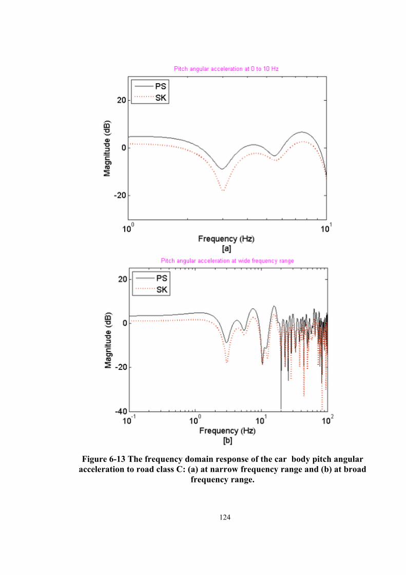
124
Figure 6-13 The frequency domain response of the car body pitch angular acceleration to road class C: (a) at narrow frequency range and (b) at broad
frequency range.

125
6.3.3.2 Simulations of ride comfort in the time domain
In this section, vehicle reaction to the road profile input by the passive and the
proposed skyhook semi-active suspension systems is described. For better
visualization, the response of vehicle vertical, pitch angular acceleration and the
vertical displacement of sprung mass have been plotted separately in a short time
span in Figure 6-14 (b), Figure 6-15 (b) and Figure 6-16 (b) respectively. From
Figure 6-14 (a), Figure 6-15 (a) and Figure 6-16 (a), it is quite apparent that the
vehicle vertical, pitch angular accelerations and the vertical displacement of the
vehicle front left sprung mass of the SK system are better than the PS system.
Compared to the passive suspension system, the NV (Normalize body vertical
acceleration) and NP (Normalized pitch angular acceleration) of the skyhook
controlled suspension system have decreased by 18.32% and 14.92%
respectively.
However the road handling performance of the SK controlled suspension
system has decreased by only 1.68% compared to the passive suspension system.
But the SK system’s weighted RMS acceleration value of the sprung mass
obtained in this simulation is 0.72 which is within the acceptable range of
international code ISO 2631 [143]. Since the vehicle is traversing on a straight
road, the differences in roll angular and lateral acceleration of both systems are
negligible. Hence, the skyhook controlled suspension system is able to improve
ride comfort of the vehicle effectively while the vehicle is moving on road class
C.

126
Figure 6-14 The time domain response of vehicle body vertical acceleration to road class C: (a) full trajectory and (b) short time span.

127
Figure 6-15 The time domain response of vehicle pitch angular acceleration to road class C: (a) full trajectory and (b) short time span.

128
Figure 6-16 The time domain response of the vehicle sprung mass m1 vertical displacement to road class C: (a) full trajectory and (b) short time
span.

129
6.3.4 Simulation on combined road
In this section, the performance of the proposed skyhook controller on a
combined road surface (generated using the three classes A, B and C of road
profiles where each class lasts for 20s) is evaluated in the frequency domain and
time domain separately.
6.3.4.1 Simulations of ride comfort in the frequency domain
The ride performance of the integrated semi-active suspension system in the
frequency domain is evaluated in this section. The response of the vehicle body
vertical acceleration and pitch angular acceleration at 0 Hz to 10 Hz have been
plotted separately in a short time span in Figure 6-17 (a) and Figure 6-18 (a)
respectively.
From Figure 6-17 (b) and Figure 6-18 (b), it is quite evident that the
vehicle body vertical acceleration and pitch angular acceleration of the SK
system remain closer to 0 db than the PS system at a wide range of frequencies,
particularly in the region where humans are more sensitive to vibrations (Figure
6-17 (a) and Figure 6-18 (a)).

130
Figure 6-17. The frequency domain response of the car body vertical acceleration to the combined road: (a) at narrow frequency range and (b) at
broad frequency range.

131
Figure 6-18. The frequency domain response of the car body pitch angular acceleration to the combined road: (a) at narrow frequency range and (b) at
broad frequency range.

132
6.3.4.2 Simulations of ride comfort in the time domain
In this section, vehicle reaction to the road profile input by the passive and the
proposed skyhook semi-active suspension systems are described. For better
visualization, the response of vehicle vertical, pitch angular acceleration and the
vertical displacement of sprung mass have been plotted separately in a short time
span in Figure 6-19 (b), Figure 6-20 (b) and Figure 6-21 (b) respectively. From
Figure 6-19 (a), Figure 6-20 (a) and Figure 6-21 (a), it is quite apparent that the
vehicle vertical, pitch angular accelerations and the vertical displacement of the
vehicle front left sprung mass of the SK system are better than the PS system.
Compared to the passive suspension system, the NV (Normalize body vertical
acceleration) and NP (Normalized pitch angular acceleration) of the skyhook
controlled suspension system have decreased by 18.92% and 14.73%
respectively.
However the road handling performance of the SK controlled suspension
system has decreased by only 2.08% compared to the passive suspension system.
But the SK system’s weighted RMS acceleration value of the sprung mass
obtained in this simulation is 0.79 which is within the acceptable range of
international code ISO 2631 [143]. Since the vehicle is traversing on a straight
road, the differences in roll angular and lateral acceleration of both systems are
negligible. Hence, the skyhook controlled suspension system is able to improve
ride comfort of the vehicle effectively while the vehicle is moving on combined
road surface.

133
Figure 6-19 The time domain response of vehicle body vertical acceleration to the combined road: (a) full trajectory and (b) short time span.

134
Figure 6-20 The time domain response of vehicle pitch angular acceleration to the combined road: (a) full trajectory and (b) short time span.

135
Figure 6-21 The time domain response of the vehicle sprung mass m1 vertical displacement to the combined road: (a) full trajectory and (b) short
time span.

136
6.4 Simulation with skyhook and direct tilt controller
The objective of this section is to study the response of the vehicle when it is
tilted due to steering angle and road bank angle. The tilting mode of the system
was evaluated using the MATLAB and SIMULINK simulation where the direct
tilt control is activated along with the proposed skyhook controller.
In this simulation, the vehicle experienced road class C defined by
ISO8608 described in Section 4.3. The vehicle is travelling in a same speed of 10
meter per second. The vehicle’s trajectory is set by four driving scenarios
depicted in Section 5.5 and the response of the vehicle travelling on road class C
with each scenario described below.
6.4.1 Simulation on driving scenario one
In this section, vehicle reaction to driving scenario one using the PS and the
SKDT semi-active suspension system is described. Figure 6-22(a) shows the
response of the vehicle’s desired tilting angle (faiD) for the steering input signal
(Delta) and the road bank angle (β) according to the designed Direct Tilt Control
system. The required actuator force to tilt the vehicle according to the desired
tilting angle is depicted in Figure 6-43(b).

137
Figure 6-22 The response of steering and bank angle in driving scenario one:
(a) Desired tilting angle (b) Required actuator force.
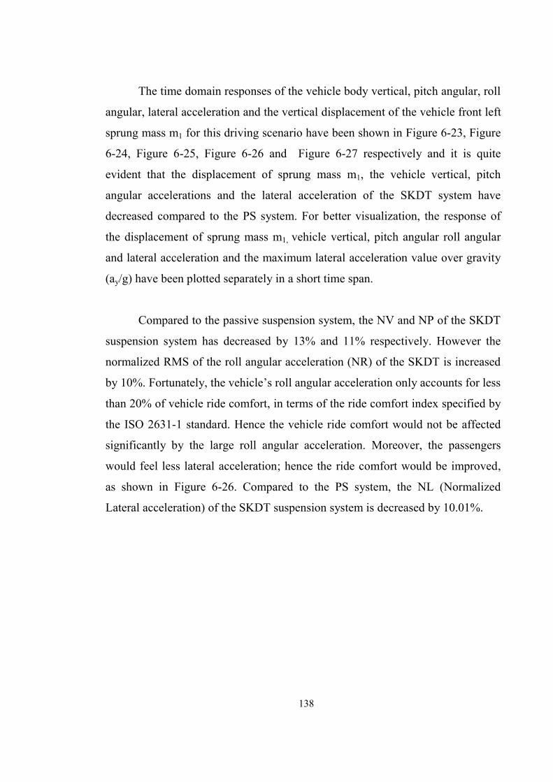
138
The time domain responses of the vehicle body vertical, pitch angular, roll
angular, lateral acceleration and the vertical displacement of the vehicle front left
sprung mass m1 for this driving scenario have been shown in Figure 6-23, Figure
6-24, Figure 6-25, Figure 6-26 and Figure 6-27 respectively and it is quite
evident that the displacement of sprung mass m1, the vehicle vertical, pitch
angular accelerations and the lateral acceleration of the SKDT system have
decreased compared to the PS system. For better visualization, the response of
the displacement of sprung mass m1, vehicle vertical, pitch angular roll angular
and lateral acceleration and the maximum lateral acceleration value over gravity
(ay/g) have been plotted separately in a short time span.
Compared to the passive suspension system, the NV and NP of the SKDT
suspension system has decreased by 13% and 11% respectively. However the
normalized RMS of the roll angular acceleration (NR) of the SKDT is increased
by 10%. Fortunately, the vehicle’s roll angular acceleration only accounts for less
than 20% of vehicle ride comfort, in terms of the ride comfort index specified by
the ISO 2631-1 standard. Hence the vehicle ride comfort would not be affected
significantly by the large roll angular acceleration. Moreover, the passengers
would feel less lateral acceleration; hence the ride comfort would be improved,
as shown in Figure 6-26. Compared to the PS system, the NL (Normalized
Lateral acceleration) of the SKDT suspension system is decreased by 10.01%.

139
Figure 6-23 The vehicle body vertical acceleration for driving scenario one: (a) full trajectory and (b) short time span.

140
Figure 6-24 The pitch angular acceleration for driving scenario one: (a) full trajectory and (b) short time span.

141
Figure 6-25 The roll angular acceleration for driving scenario one: (a) full trajectory and (b) short time span.

142
Figure 6-26 The lateral acceleration for driving scenario one: (a) full trajectory and (b) short time span.

143
Figure 6-27 The vehicle sprung mass m1‘s vertical displacement for driving scenario one: (a) full trajectory and (b) short time span.

144
Figure 6-28 The rollover threshold in driving scenario one: (a) full trajectory and (b) short time span.

145
If the body of the vehicle is parallel with the ground surface, its rollover
threshold becomes a function of the vehicle’s track width (t) and the centre of
gravity height (h) as depicted in equation (5.17). The maximum allowable
rollover threshold of this vehicle is 1.45. The rollover threshold defines the
maximum lateral acceleration value over gravity (ay/g) that the vehicle would be
able to reach before tipping over. From Figure 6-28 (a) and (b), it is apparent that
(ay/g) never exceeds the maximum allowable rollover threshold of this vehicle.
Hence the vehicle remains stable throughout the trajectory of this driving
scenario.
However the road handling performance of the skyhook controlled
suspension system has decreased by only 2.3% compared to the passive
suspension system. But the SKDT system’s weighted RMS acceleration value of
the sprung mass obtained in this simulation is 0.71 which is within the acceptable
range. Hence, the integrated suspension system is able to improve ride comfort of
the vehicle effectively while the vehicle is moving on road class C with this
driving scenario.
6.4.2 Simulation on driving scenario two
In this section, vehicle reaction to driving scenario two using the PS and the
SKDT semi-active suspension system is described. Figure 6-29(a) shows the
response of the vehicle’s desired tilting angle for the steering input signal and the
road bank angle according to the designed Direct Tilt Control system. The
required actuator force to tilt the vehicle according to the desired tilting angle is
depicted in Figure 6-29(b).

146
Figure 6-29 The response of steering and bank angle in driving scenario
two: (a) Desired tilting angle (b) Required actuator force.
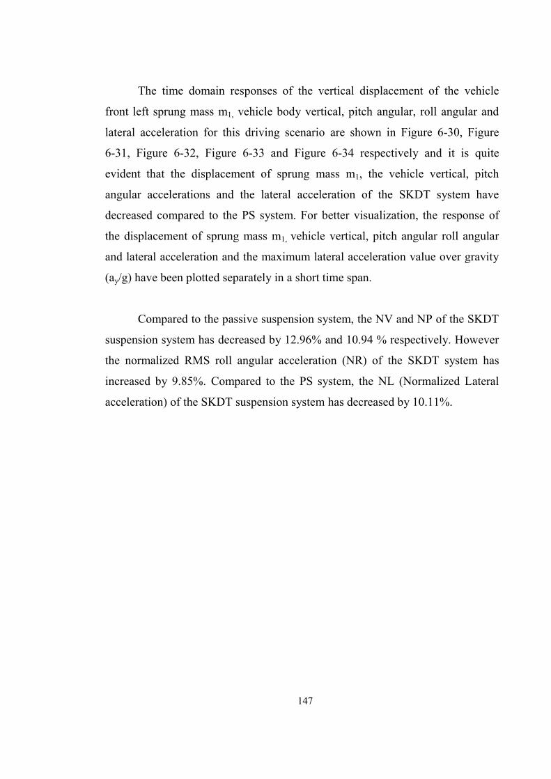
147
The time domain responses of the vertical displacement of the vehicle
front left sprung mass m1, vehicle body vertical, pitch angular, roll angular and
lateral acceleration for this driving scenario are shown in Figure 6-30, Figure
6-31, Figure 6-32, Figure 6-33 and Figure 6-34 respectively and it is quite
evident that the displacement of sprung mass m1, the vehicle vertical, pitch
angular accelerations and the lateral acceleration of the SKDT system have
decreased compared to the PS system. For better visualization, the response of
the displacement of sprung mass m1, vehicle vertical, pitch angular roll angular
and lateral acceleration and the maximum lateral acceleration value over gravity
(ay/g) have been plotted separately in a short time span.
Compared to the passive suspension system, the NV and NP of the SKDT
suspension system has decreased by 12.96% and 10.94 % respectively. However
the normalized RMS roll angular acceleration (NR) of the SKDT system has
increased by 9.85%. Compared to the PS system, the NL (Normalized Lateral
acceleration) of the SKDT suspension system has decreased by 10.11%.

148
Figure 6-30 The vehicle sprung mass m1‘s vertical displacement for driving scenario two: (a) full trajectory and (b) short time span.

149
Figure 6-31 The vehicle body vertical acceleration for driving scenario two: (a) full trajectory and (b) short time span.
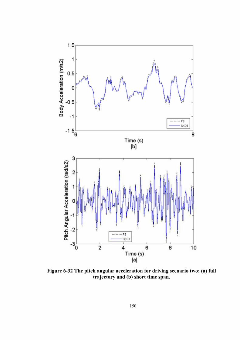
150
Figure 6-32 The pitch angular acceleration for driving scenario two: (a) full trajectory and (b) short time span.

151
Figure 6-33 The roll angular acceleration for driving scenario two: (a) full trajectory and (b) short time span.

152
Figure 6-34 The lateral acceleration for driving scenario two: (a) full trajectory and (b) short time span.
153
Figure 6-35 The rollover threshold in driving scenario two: (a) full trajectory and (b) short time span.

154
If the body of the vehicle is parallel with the ground surface, its rollover
threshold becomes a function of the vehicle’s track width (t) and the centre of
gravity height (h) as depicted in equation (5.17). The maximum allowable
rollover threshold of this vehicle is 1.45. The rollover threshold defines the
maximum lateral acceleration value over gravity (ay/g) that the vehicle would be
able to reach before tipping over. From Figure 6-35(a) and (b), it is apparent that
(ay/g) never exceeds the maximum allowable rollover threshold of this vehicle.
Hence the vehicle remains stable throughout the trajectory of this driving
scenario.
However the road handling performance of skyhook controlled suspension
system has decreased by only 2.33% compared to the passive suspension system.
But the SKDT system’s weighted RMS acceleration value of the sprung mass
obtained in this simulation is 0.76 which is within the acceptable range. Hence,
the integrated suspension system is able to improve ride comfort of the vehicle
effectively while the vehicle is moving on road class C with this driving scenario.
6.4.3 Simulation on driving scenario three
In this section, vehicle reaction to the driving scenario using the PS and the
SKDT semi-active suspension systems is described. Figure 6-36(a) shows the
response of the faiD for the input signal Delta and the β according to the
designed Direct Tilt Control. The required actuator force to tilt the vehicle
according to the desired tilting angle is depicted in Figure 6-36(b).

155
Figure 6-36 The response of steering and bank angle in driving scenario
three: (a) Desired tilting angle (b) Required actuator force.

156
The time domain responses of the vertical displacement of the vehicle
front left sprung mass m1, vehicle body vertical, pitch angular, roll angular and
lateral acceleration for this driving scenario are shown in Figure 6-37, Figure
6-38, Figure 6-39, Figure 6-40 and Figure 6-41respectively and it is quite evident
that the displacement of sprung mass m1, the vehicle vertical, pitch angular
accelerations and the lateral acceleration of the SKDT system have decreased
compared to the PS system. For better visualization, the response of the
displacement of sprung mass m1, vehicle vertical, pitch angular roll angular and
lateral acceleration and the maximum lateral acceleration value over gravity
(ay/g) have been plotted separately in a short time span.
Compared to the passive suspension system, the NV and NP of the SKDT
suspension system have decreased by 12.66% and 10.44 % respectively.
However the normalized RMS roll angular acceleration (NR) of the SKDT
system has increased by 9.95%. Compared to the PS system, the NL (Normalized
Lateral acceleration) of the SKDT suspension system has decreased by 10.61%.

157
Figure 6-37 The vehicle sprung mass m1‘s vertical displacement for driving
scenario three: (a) full trajectory and (b) short time span.

158
Figure 6-38 The vehicle body vertical acceleration for driving scenario three: (a) full trajectory and (b) short time span.

159
Figure 6-39 The pitch angular acceleration for driving scenario three: (a) full trajectory and (b) short time span.
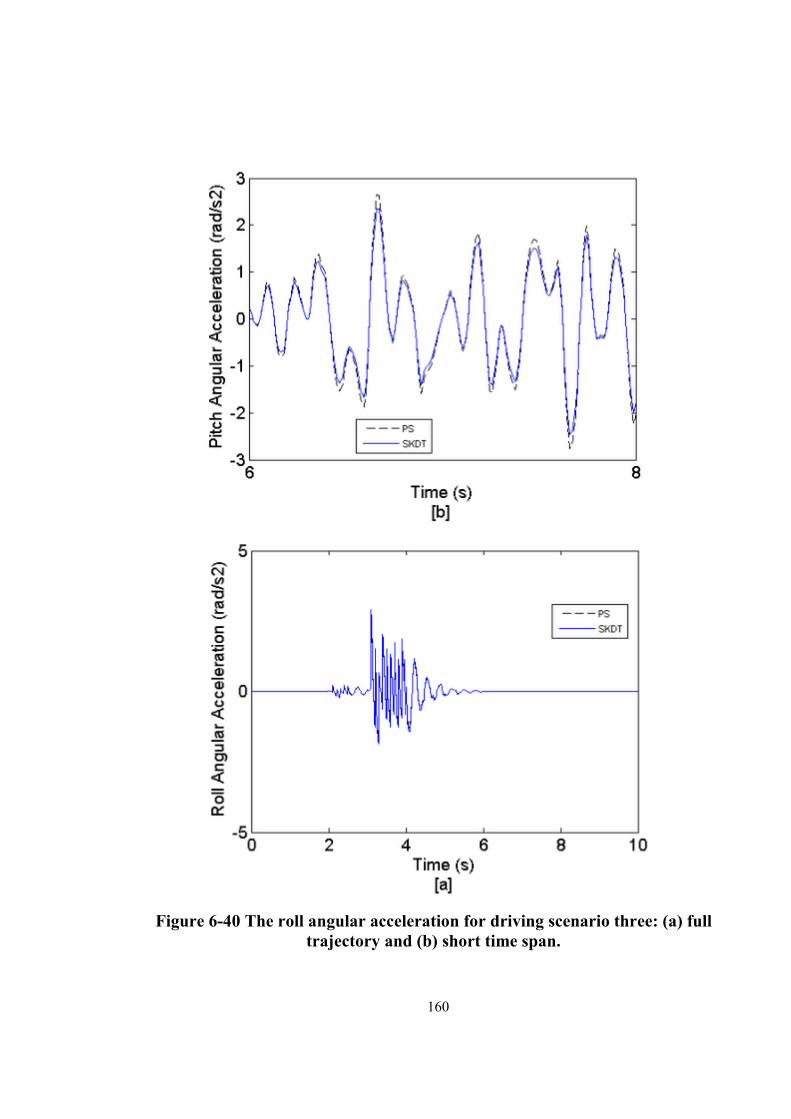
160
Figure 6-40 The roll angular acceleration for driving scenario three: (a) full trajectory and (b) short time span.

161
Figure 6-41 The lateral acceleration for driving scenario three: (a) full trajectory and (b) short time span.

162
Figure 6-42 The rollover threshold in driving scenario three: (a) full trajectory and (b) short time span.
If the body of the vehicle is parallel with the ground surface, its rollover
threshold becomes a function of the vehicle’s track width (t) and the centre of

163
gravity height (h) as depicted in equation (5.17). The maximum allowable
rollover threshold of this vehicle is 1.45. The rollover threshold defines the
maximum lateral acceleration value over gravity (ay/g) that the vehicle would be
able to reach before tipping over. From Figure 6-42(a) and (b), it is apparent that
(ay/g) never exceeds the maximum allowable rollover threshold of this vehicle.
Hence the vehicle remains stable throughout the trajectory of this driving
scenario.
However the road handling performance of the skyhook controlled
suspension system has decreased by only 2.23% compared to the passive
suspension system. But the SKDT system’s weighted RMS acceleration value of
the sprung mass obtained in this simulation is 0.69 which is within the acceptable
range. Hence, the integrated suspension system is able to improve ride comfort of
the vehicle effectively while the vehicle is moving on road class C with this
driving scenario.
6.4.4 Simulation on driving scenario four
In this section, vehicle reaction to the driving scenario using the PS and the
SKDT semi-active suspension system is described. Figure 6-43 (a) shows the
response of the vehicle’s desired tilting angle (faiD) for the steering input signal
(Delta) and the road bank angle (β) according to the designed Direct Tilt Control
system. The required actuator force to tilt the vehicle according to the desired
tilting angle is depicted in Figure 6-43 (b).

164
Figure 6-43 The response of steering and bank angle in driving scenario
four: (a) Desired tilting angle (b) Required actuator force.

165
The time domain responses of the vertical displacement of the vehicle
front left sprung mass m1, vehicle body vertical, pitch angular, roll angular and
lateral acceleration for this driving scenario are shown in Figure 6-44, Figure
6-45, Figure 6-46, Figure 6-47 and Figure 6-48 respectively and it is quite
evident that the displacement of sprung mass m1, the vehicle vertical, pitch
angular accelerations and the lateral acceleration of the SKDT system have
decreased compared to the PS system. For better visualization, the response of
the displacement of sprung mass m1, vehicle vertical, pitch angular roll angular
and lateral acceleration and the maximum lateral acceleration value over gravity
(ay/g) have been plotted separately in a short time span.
Compared to the passive suspension system, the NV and NP of the SKDT
suspension system has decreased by 12.99% and 10.99 % respectively. However
the normalized RMS roll angular acceleration (NR) of the SKDT system has
increased by 9.99%. Fortunately, the vehicle’s roll angular acceleration only
accounts for less than 20% of vehicle ride comfort, in terms of ride comfort index
specified by the ISO 2631-1 standard. Hence the vehicle ride comfort would not
be affected significantly by the large roll angular acceleration. Moreover, the
passengers would feel less lateral acceleration; hence the ride comfort would be
improved, as shown in Figure 6-48. Compared to the PS system, the NL
(Normalized Lateral acceleration) of the SKDT suspension system has decreased
by 10%.

166
Figure 6-44 The vehicle sprung mass m1‘s vertical displacement for driving
scenario four: (a) full trajectory and (b) short time span.

167
Figure 6-45 The vehicle body vertical acceleration for driving scenario four:
(a) full trajectory and (b) short time span.

168
Figure 6-46 The pitch angular acceleration for driving scenario four: (a) full
trajectory and (b) short time span.

169
Figure 6-47 The roll angular acceleration for driving scenario four: (a) full
trajectory and (b) short time span.

170
Figure 6-48 The lateral acceleration for driving scenario four: (a) full trajectory and (b) short time span.

171
Figure 6-49 The rollover threshold in driving scenario four: (a) full trajectory and (b) short time span.

172
If the body of the vehicle is parallel with the ground surface, its rollover
threshold becomes a function of the vehicle’s track width (t) and the centre of
gravity height (h) as depicted in equation (5.17). The maximum allowable
rollover threshold of this vehicle is 1.45. The rollover threshold defines the
maximum lateral acceleration value over gravity (ay/g) that the vehicle would be
able to reach before tipping over. From Figure 6-49 (a) and (b), it is apparent that
(ay/g) never exceeds the maximum allowable rollover threshold of this vehicle.
Hence the vehicle remains stable throughout the trajectory of this driving
scenario.
However the road handling performance of the skyhook controlled
suspension system has decreased by only 2% compared to the passive suspension
system. But the SKDT system’s weighted RMS acceleration value of the sprung
mass obtained in this simulation is 0.72 which is within the acceptable range.
6.5 Simulation Summary
The objective of this section is to summarize the evaluation of the SK system
(the proposed skyhook suspension system) and the SKDT system where the
direct tilt control is activated along with the proposed skyhook controller in the
same simulation. The performance of the SK and SKDT systems are compared to
the PS system (the passive suspension system). In this simulation, the vehicle
experienced road class C defined by ISO8608 described in Section 5.5. The
vehicle trajectory defined by the driving scenario four (Section 5.5). This driving
scenario has been used as if the vehicle experienced both left and right turns. The
frequency and time domain analysis are presented separately in the following
sections.

173
6.5.1 Simulations of ride comfort in the frequency domain
Figure 6-50 and Figure 6-51 show the frequency responses of the vehicle
vertical, pitch angular and roll angular acceleration to the road disturbance class
C. For better visualization, the responses of vehicle vertical, pitch angular and
roll angular accelerations at 0 Hz to 10 Hz have been plotted separately in a short
time span in Figure 6-50 (a), Figure 6-51 (a) and Figure 6-52 (a) respectively.
Study shows that human beings are very sensitive to the vertical motion in
the frequency range of 4 to 8Hz [134]. So while designing a vehicle suspension
system, sprung mass acceleration tolerance should be kept to a minimum in the
frequency range mentioned above. From Figure 6-50 (b) and Figure 6-51 (b), it is
quite evident that the vehicle body vertical acceleration and pitch angular
acceleration of the SK and SKDT systems remained closer to 0 db than the PS
system at a wide range of frequencies, especially at frequencies where humans
are more sensitive to vibrations (Figure 6-50 (a) and Figure 6-51 (a)).
However the frequency responses of roll angular acceleration of the SK
and SKDT systems have deteriorated compared to the PS system as shown in
Figure 6-52. Fortunately, the vehicle’s roll angular acceleration only accounts for
less than 20% of vehicle ride comfort, in terms of ride comfort index specified by
the ISO 2631-1 standard. Hence the vehicle ride comfort would not be affected
significantly by the large roll angular acceleration. Moreover, the passengers
would feel less lateral acceleration; hence the ride comfort would be improved
which will be shown later in time domain analysis.
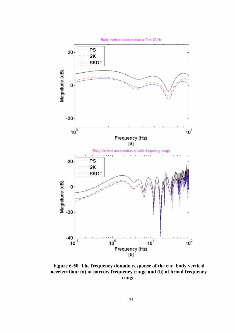
174
Figure 6-50. The frequency domain response of the car body vertical acceleration: (a) at narrow frequency range and (b) at broad frequency
range.

175
Figure 6-51. The frequency domain response of the car body pitch angular acceleration: (a) at narrow frequency range and (b) at broad frequency
range.

176
Figure 6-52. The frequency domain response of the car body roll angular acceleration: (a) at narrow frequency range and (b) at broad frequency
range.

177
6.5.2 Simulations of ride comfort in the time domain
Figure 6-53 The response of steering and bank angle in driving scenario four
and road class C: (a) Desired tilting angle (b) Required actuator force.
178
In this section, vehicle reaction to the driving scenario using the PS and the
SKDT semi-active suspension system is described. Figure 6-53(a) shows the
response of the vehicle’s desired tilting angle (faiD) for the steering input signal
(Delta) and the road bank angle (β) according to the designed Direct Tilt Control
(Section 5.4.1). The required actuator force to tilt the vehicle according to the
desired tilting angle is depicted in Figure 6-53(b).
The time domain responses of the vehicle body vertical, pitch angular, roll
angular, lateral acceleration and the vertical displacement of the vehicle front left
sprung mass m1 for this driving scenario are shown in Figure 6-54, Figure 6-55 ,
Figure 6-56, Figure 6-57 and Figure 6-58 respectively and it is quite apparent
that the displacement of sprung mass m1, the vehicle vertical, pitch angular
accelerations and the lateral acceleration of the SK and SKDT systems have
decreased compared to the PS system. For better visualization, the responses of
the displacement of sprung mass m1, vehicle vertical, pitch angular roll angular
and lateral acceleration and the maximum lateral acceleration value over gravity
(ay/g) have been plotted separately in a short time span.
If the body of the vehicle is parallel with the ground surface, its rollover
threshold becomes a function of the vehicle’s track width (t) and the centre of
gravity height (h) as depicted in equation (5.9). The maximum allowable rollover
threshold of this vehicle is 1.4578. The rollover threshold defines the maximum
lateral acceleration value over gravity (ay/g) that the vehicle would be able to
reach before tipping over. From Figure 6-59 (a) and (b), it is clear that (ay/g)
never exceeds the maximum allowable rollover threshold of this vehicle. Hence
the vehicle remains stable throughout the trajectory of this driving scenario.

179
Figure 6-54 The vehicle body vertical acceleration for driving scenario four and road class C: (a) full trajectory and (b) short time span.

180
Figure 6-55 The pitch angular acceleration for driving scenario four and road class C: (a) full trajectory and (b) short time span.

181
Figure 6-56 The roll angular acceleration for driving scenario four and road class C: (a) full trajectory and (b) short time span.

182
Figure 6-57 The lateral acceleration for driving scenario four and road class C: (a) full trajectory and (b) short time span.

183
Figure 6-58 The vehicle sprung mass m1‘s vertical displacement for driving scenario four and road class C: (a) full trajectory and (b) short time span.

184
Figure 6-59 The rollover threshold in driving scenario four and road class C: (a) full trajectory and (b) short time span.

185
Compared to the passive suspension system, the normalized RMS body
vertical acceleration (NV) of the SK and SKDT suspension systems have
decreased by 10.68% and 12.99% respectively as shown in Figure 6-60. The
normalized RMS pitch angular accelerations (NP) of the SK and SKDT
suspension systems have decreased by 9.29% and 10.99% respectively (Figure
6-61).
However Figure 6-62 shows that the normalized RMS roll angular
acceleration (NR) of the SK and SKDT systems have increased by 0.61% and
9.99%. Fortunately, the vehicle’s roll angular acceleration only accounts for less
than 20% of vehicle ride comfort, in terms of ride comfort index specified by the
ISO 2631-1 standard. Hence the vehicle ride comfort would not be affected
significantly by the large roll angular acceleration. Moreover, the passengers
would feel less lateral acceleration; hence the ride comfort would be improved.
Compared to the PS system, the NL (Normalized Lateral acceleration) of the SK
and SKDT suspension systems have decreased by 0.46% and 10% respectively
(Figure 6-63).
As shown in Figure 6-64, the road handling performance of the SK and
SKDT systems have decreased by only 2.09% and 2% compared to the passive
suspension system. But the weighted RMS acceleration value of the sprung mass
obtained in this simulation is 0.65 and 0.72 for the SK and SKDT systems
respectively which are within the acceptable range of international code ISO
2631 [143]. Hence, the SK and SKDT suspension systems are able to improve
ride comfort of the vehicle effectively while the vehicle is moving on road class
C.

186
Figure 6-60 Vehicle body vertical acceleration comparison.
Figure 6-61 Vehicle body pitch angular acceleration comparison.

187
Figure 6-62 Vehicle body roll angular acceleration comparison.
Figure 6-63.Vehicle body lateral acceleration comparison.

188
Figure 6-64 Vehicle road handling performance comparison.
6.6 Conclusions
This chapter describes the conclusion reached from the analysis of the
simulations that were carried out to investigate the proposed skyhook control
suspension system and the designed Direct Tilt Control system. The SK and
SKDT systems were applied to the dynamic model of a full car which considers
the road bank angle. At first, the responses of the dynamic model of the full car
on different road classes A, B and C defined by ISO8608 and also combined road
profile described in Section (4.3) were observed. In this section, PS and SK
systems were analysed separately. The behaviour of the vehicle body vertical
acceleration and pitch angular acceleration were examined in the frequency
domain. While travelling on all the road profiles, it has been ascertained that, the
vehicle body vertical acceleration and pitch angular acceleration of the SK
system remains closer to 0 db than the PS system at a wide range of frequencies,
particularly in the region where humans are more sensitive to vibrations.

189
The time domain analysis was also carried out on the full car model using
the PS and the SK systems separately. In this sub-section, vertical displacement
of the vehicle front left sprung mass m1, vehicle body vertical acceleration and
pitch angular acceleration were assessed. NV (Normalize body vertical
acceleration) and NP (Normalized pitch angular acceleration) were calculated
and the result is that the SK system significantly reduced the vehicle body
vertical acceleration and pitch angular acceleration in all instances compared to
the PS system. However the road handling performance of the SK controlled
suspension system decreased slightly compared to the passive suspension system.
But the SK system’s weighted RMS acceleration value of the sprung mass
obtained in this simulation was always within the acceptable range of
international code ISO 2631 [143]. Since the vehicle was traversing on a straight
road, the differences in roll angular and lateral acceleration of both systems were
negligible in this analysis.
Subsequently, the simulations of the dynamic model of the full car in
different driving scenarios (described in Section (5.4)) were carried out using the
SKDT system. Vehicle reaction to the driving scenarios of both the PS and the
SKDT semi-active suspension systems were described in this section. The
response of the vehicle’s desired tilting angle (faiD) for the corresponding
steering input signal (Delta) and the road bank angle (β) have been shown. The
required actuator force to tilt the vehicle according to the desired tilting angle
was also observed.
Here the time domain responses of the vertical displacement of the vehicle
front left sprung mass m1, vehicle body vertical, pitch angular, roll angular and
lateral acceleration for each driving scenario were shown and it was quite evident
that the displacement of sprung mass m1, the vehicle vertical, pitch angular
accelerations and the lateral acceleration of the SKDT system has decreased

190
compared to the PS system. Compared to the passive suspension system, the NV
and NP of the SKDT suspension system has decreased significantly. However
the normalized RMS of the roll angular acceleration (NR) of the SKDT system
has increased significantly for the tilting action. Fortunately, the vehicle’s roll
angular acceleration only accounts for less than 20% of vehicle ride comfort, in
terms of ride comfort index specified by the ISO 2631-1 standard. Hence the
vehicle ride comfort would not be affected significantly by the large roll angular
acceleration. Moreover, the appropriate tilting action reduces the lateral
acceleration experienced by passengers and improved the vehicle ride comfort, as
the NL (Normalized Lateral acceleration) of the SKDT suspension system has
decreased by 10.01% compared to the PS system. The stability of the resulting
closed loop system was then investigated.
At the end of this chapter, the combined simulation was discussed. Road
class C and driving scenario four were used to evaluate the performance of the
PS, SK and SKDT systems. It has been demonstrated that the proposed skyhook
control system on its own can improve the vehicle ride comfort keeping the road
handling performance within an acceptable range. The SKDT system shows that
this control strategy is capable of tilting a vehicle inward which would act against
the lateral acceleration resulting from steering manoeuvres. The designed SKDT
system was capable of maintaining the system’s tilt state by keeping the vehicle
stable and safe from rollover. This research has indicated the potential of the
SKDT suspension system for improving cornering performances of vehicles and
paves the way for future work on an integrated system for chassis control.

191
Chapter 7 Experimental analysis of full car model
7.1 Overview
In this chapter, the analysis of the dynamics of a full car model is presented. It
incorporates the response of the Quanser quarter-car suspension plant as one of
the four wheels of the full car model. Section 7.2 describes the environment of
the experimental analysis and the parameters of the full car that emulated from
the Quanser quarter-car suspension plant. The vehicle performance analysis
using the Quanser quarter-car suspension plant at the front left and rear right
wheel of the full car model is presented separately in Sections 7.3 and 7.4. The
performance of the combined approach where the proposed skyhook controller is
activated along with the direct tilt control is evaluated in Sections 7.3 and 7.4 at
frequency domain and time domain.
7.2 Experimental environment
One objective of the suspension control system design in this research is to tilt
the vehicle inward when it is steered. The proposed skyhook control and the
tilting mode of the system were investigated using the Quanser suspension plant.
The real time simulation environment with the experimental model was setup in
such a way that the road profile input interacting with the front left wheel of the
full vehicle model was fed into the Quanser quarter-car suspension plant using
the Simulink model illustrated in Figure 7-1. The output of the Quanser
suspension plant was then fed back to the full car model to complete the real time
simulation. An analysis was carried out using the Quanser quarter-car suspension
plant as the rear right wheel of the full car model. The Quanser suspension
system has three masses, each supported by two springs as shown in Figure 4-8.
The vehicle body is represented by the upper mass (blue) supported above the

192
suspension while the middle mass (red) represents one of the vehicle’s wheels. A
programmable motor is used to actuate the upper mass. The lower plate (silver)
emulates the road surface by moving vertically. The performance criteria can be
formulated into a mathematical model. The Ride Comfort is measurable through
an accelerometer located on the sprung mass. Suspension Travel is measured
using a linear capstan mechanism. The parameters that have been used in this
analysis are listed in Table 7-1.
The objective of this section is to describe the evaluation of the SK system
(the proposed skyhook suspension system) and the SKDT system (the direct tilt
control is activated along with the proposed skyhook controller). The
performance of the SK and SKDT systems are compared to the PS system (the
passive suspension system). In this analysis, the vehicle experienced road class C
defined by ISO8608 described in Section (4.3). The vehicle trajectory is defined
by driving scenario four (Section (5.5)). This driving scenario has been used as
the vehicle experiences both left and right turns. The vehicle performance
analysis using the Quanser quarter-car suspension plant at the front left and rear
right wheel of the full car model is presented separately in the following sections.

193
Table 7-1 Nominal parameter values used in the experiment.
Parameter Definition Values
mi(i=1,2,3,4) Vehicle un-sprung masses 1 [kg]
m Sprung mass 10 [kg]
Mt Total mass of the vehicle 14 [kg]
ki1 (i=1,2,3,4) Tyre spring coefficient 2500 [N/m]
Ki2 (i=1,2,3,4) Suspension spring coefficient 900 [N/m]
ct1~ ct4 Tyre damping coefficient 5 [N-s/m]
c1~ c4 Suspension damping coefficient 7.5 [N-s/m]
a Distance from C.G. to front wheel 0.732 [m]
b Distance from C.G. to rear wheel 0.982[m]
c, d Half of wheel base 0.452[m]
h Height of C.G of the vehicle 0.35[m]
Cαf , Cαr Cornering stiffness of the tyre 16339[N/rad]
Ix Roll moment of inertial 1.13 [kg m2]
Iy Pitch moment of inertial 4.79[kg m2]
Iz Yaw moment of inertial 5.34[kg m2]
g Gravity acceleration 9.8 [m/s2]

194
U = [ zr ; Fc ]
0
s8
Body wrt base
Vehicle Body
Body wrt base
Road
suspension_comp
zus
Tire_comp1
Suspension
Cmd Road (m1,x1)
Road simulator
zr
Road SurfaceGenerator Y
u
x_obs
Observer Dynamics1
Manual Switch
HILWrite
Digital
HIL Write Digital(HIL-1)
HIL InitializeHIL-1 (qpid_e-0)
[zr]
[Fc]
[accel]
Goto7
[zr]
[susp_comp]
[tire2base]
[body2base]
[road]
[tire_comp]
[Zr_measured]
[x_actual]
[y_measured][x_measured]
[x_obs_m]
[Fc]
[zr]
[susp_comp]
[x_sim]
[susp_comp]
[body2base]
[tire2base]
[tire_comp]
[body2base]
From13
[accel]
[road]
[x_measured]
In1Out2
Diff4
In1Out2
Diff1
F(N)
Control Actuator
(0 0 0 0 1)
Constant
skyhookMod
C-mex S-Function3
Accel
Accelerometer
U
zr_measured
x_actual
y _measured
SuspensionActual Plant
Figure 7-1 Quanser Simulink Model.

195
Figure 7-2 Quanser Intelligent Suspension Plant.
7.3 Quanser plant at front left suspension
In this section, the experimental analysis carried out on the full car suspension
system is described. Here the Quanser suspension plant is considered to be in use
at the front left suspension of the full car suspension model.

196
Figure 7-3 The vehicle front left sprung mass vertical displacement.
Figure 7-3 shows that there is a slight difference in the vehicle front left
sprung mass vertical displacement in the the simulation environment and
experimental setup. This is because the response time of the experimental and
simulation environment are slightly different. But the comparison between the
simulation and experimental analysis has not been carried out in this section as
the simulation of a full car model similar to a standard production vehicle has
been carried out in a previous chapter already. The frequency domain analysis of
the vehicle vertical, pitch angular and roll angular acceleration responses to road
disturbance class C has been presented at Section 7.3.1. The response of the
vehicle’s desired tilting angle (faiD) for the steering input signal (Delta) and the
road bank angle (β) according to the designed Direct Tilt Control system has
been described at Section 7.3.2. In this sub section the time domain analysis has
also been conducted on the vehicle body vertical, pitch angular, roll angular,
lateral acceleration and vehicle front left sprung mass vertical displacement.

197
7.3.1 Experiments of ride comfort in the frequency domain
Figure 7-4 and Figure 7-5 show the frequency responses of the vehicle vertical,
pitch angular and roll angular acceleration in response to road disturbance class
C. For better visualization, the responses of vehicle vertical, pitch angular and
roll angular accelerations at 0 Hz to 10 Hz have been plotted separately in a short
time span in Figure 7-4 (a), Figure 7-5 (a) and Figure 7-6 (a) respectively.
Studies show that human beings are very sensitive to the vertical motion
in the frequency range of 4 to 8Hz [134]. So while designing a vehicle
suspension system, sprung mass acceleration tolerance should be kept to a
minimum in the frequency range mentioned above. From Figure 7-4 and Figure
7-5, it is quite evident that the vehicle body vertical acceleration and pitch
angular acceleration of the SK and SKDT systems remained closer to 0 db than
with the PS system at a wide range of frequencies, especially at frequencies
where humans are more sensitive to vibrations (Figure 7-4 (a) and Figure 7-5
(a)).
However, the frequency responses of roll angular acceleration of the SK
and SKDT systems have deteriorated compared to the PS system as shown in
Figure 7-6. Fortunately, the roll angular acceleration of the vehicle only accounts
for less than 20% of vehicle ride comfort, in terms of the ride comfort index
specified by ISO 2631-1 standard. Hence the vehicle ride comfort would not be
affected significantly by the large roll angular acceleration. Moreover, the
passengers would feel less lateral acceleration; hence the ride comfort would be
improved. This is shown in a subsequent section in the time domain analysis.

198
Figure 7-4 The frequency response of vehicle body vertical acceleration: (a)
at narrow frequency range and (b) at broad frequency range.

199
Figure 7-5 The frequency domain response of the car body pitch angular acceleration: (a) at narrow frequency range and (b) at broad frequency
range.

200
Figure 7-6 The frequency domain response of the car body roll angular acceleration: (a) at narrow frequency range and (b) at broad frequency
range.

201
7.3.2 Experiments of ride comfort in the time domain
Figure 7-7 The response of steering and bank angle in driving scenario four
and road class C: (a) Desired tilting angle (b) Required actuator force.

202
In this section, vehicle reactions to the driving scenario using the PS and the
SKDT semi-active suspension systems are described. Figure 7-7(a) shows the
response of the vehicle’s desired tilting angle (faiD) for the steering input signal
(Delta) and the road bank angle (β) according to the designed Direct Tilt Control
system. The required actuator force to tilt the vehicle according to the desired
tilting angle is depicted in Figure 7-7(b).
The time domain responses of the vehicle body vertical, pitch angular, roll
angular, lateral acceleration and the vertical displacement of the vehicle front left
sprung mass m1 for this driving scenario are shown in Figure 7-8, Figure 7-9,
Figure 7-10, Figure 7-11 and Figure 7-12 respectively and it is quite obvious that
the displacement of sprung mass m1, the vehicle vertical, pitch angular
accelerations and the lateral acceleration of the SK and SKDT systems have
decreased compared to the PS system. For better visualization, the responses of
the displacement of sprung mass m1, vehicle vertical, pitch angular roll angular
and lateral acceleration and the maximum lateral acceleration value over gravity
(ay/g) have been plotted separately in a short time span.
If the body of the vehicle is parallel with the ground surface, its rollover
threshold becomes a function of the vehicle’s track width (t) and the centre of
gravity height (h) as depicted in equation (5.9). The maximum allowable rollover
threshold of this vehicle is 1.4578. The rollover threshold defines the maximum
lateral acceleration value over gravity (ay/g) that the vehicle would be able to
reach before tipping over. From Figure 7-13(a) and (b), it is clear that (ay/g)
never exceeds the maximum allowable rollover threshold of this vehicle. Hence
the vehicle remains stable throughout the trajectory of this driving scenario.

203
Figure 7-8 The vehicle body vertical acceleration for driving scenario four and road class C: (a) full trajectory and (b) short time span.

204
Figure 7-9 The pitch angular acceleration for driving scenario four and road class C: (a) full trajectory and (b) short time span.

205
Figure 7-10 The roll angular acceleration for driving scenario four and road class C: (a) full trajectory and (b) short time span.
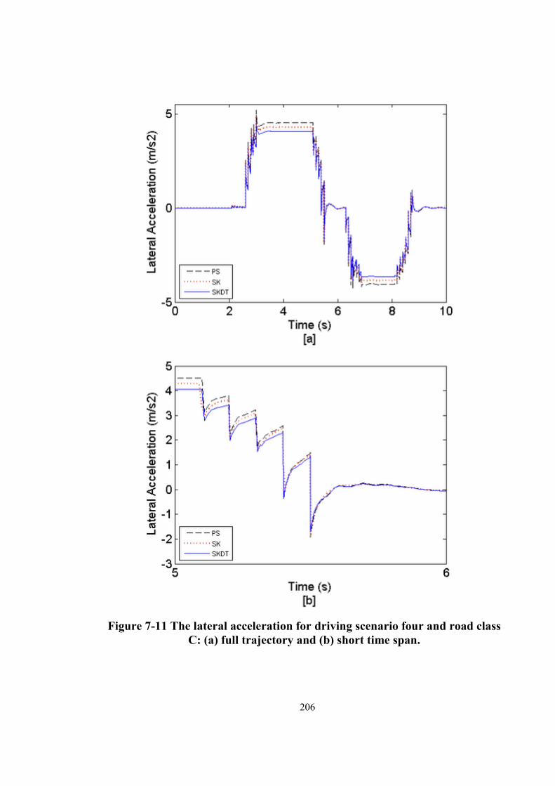
206
Figure 7-11 The lateral acceleration for driving scenario four and road class C: (a) full trajectory and (b) short time span.

207
Figure 7-12 The vehicle sprung mass m1‘s vertical displacement for driving scenario four and road class C: (a) full trajectory and (b) short time span.

208
Figure 7-13 The rollover threshold in driving scenario four and road class C: (a) full trajectory and (b) short time span.

209
Compared to the passive suspension system, the normalized RMS body
vertical acceleration (NV) of the SK and SKDT suspension systems decreased by
13.88% and 16.96% respectively as shown in Figure 7-14. The normalized RMS
pitch angular accelerations (NP) of the SK and SKDT suspension systems
decreased by 13.35% and 11% respectively (Figure 7-15).
However Figure 7-16 shows that the normalized RMS roll angular
acceleration (NR) of the SK and SKDT systems increased by 4.21% and 10%.
Fortunately, the vehicle’s roll angular acceleration only accounts for less than
20% of vehicle ride comfort, in terms of the ride comfort index specified by ISO
2631-1 standard. Hence the vehicle ride comfort would not be affected
significantly by the large roll angular acceleration. Moreover, the passengers
would feel less lateral acceleration; hence the ride comfort would be improved.
Compared to the PS system, the NL (Normalized Lateral acceleration) of the SK
and SKDT suspension systems have decreased by 5.82% and 10.22%
respectively (Figure 7-17). As shown in Figure 7-18, the road handling
performance of the SK and SKDT systems decreased by only 3.41% and 2.11%
compared to the passive suspension system which is within the acceptable range.
Hence, the SK and SKDT suspension controllers can effectively improve vehicle
ride comfort while the vehicle is moving on road class C.

210
Figure 7-14. Vehicle body vertical acceleration comparison.
Figure 7-15 Vehicle body pitch angular acceleration comparison.
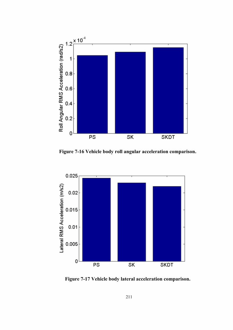
211
Figure 7-16 Vehicle body roll angular acceleration comparison.
Figure 7-17 Vehicle body lateral acceleration comparison.

212
Figure 7-18 Vehicle road handling performance comparison.
7.4 Quanser plant at rear right suspension
In this section, experimental analysis was carried out on a full car suspension
system. Here the Quanser suspension plant is considered to be in use at the rear
right suspension of the full car suspension model.

213
Figure 7-19 The vehicle rear right sprung mass vertical displacement.
Figure 7-19 shows that there is a slight difference in the vehicle rear right
sprung mass vertical displacement with the simulation environment and
experimental setup. This is because the response time of the experimental and
simulation environments is slightly different. But the comparison between the
simulation and experimental analysis is not discussed in this section as the
simulation of the full car model similar to a standard production vehicle was
discussed in the previous chapter. The frequency domain analysis of the vehicle
vertical, pitch angular and roll angular accelerations in response to the road
disturbance class C was presented in Section 7.4.1. The response of the vehicle’s
desired tilting angle (faiD) for the steering input signal (Delta) and the road bank
angle (β) according to the designed Direct Tilt Control system was described in
Section 7.4.2. In this sub section the time domain analysis has also been
presented on the vehicle body vertical, pitch angular, roll angular, lateral
accelerations and vehicle rear right sprung mass vertical displacement.

214
7.4.1 Experiments of ride comfort in the frequency domain
Figure 7-20 and Figure 7-21 show the frequency responses of the vehicle
vertical, pitch angular and roll angular acceleration to road disturbance class C.
For better visualization, the responses of vehicle vertical, pitch angular and roll
angular accelerations at 0 Hz to 10 Hz have been plotted separately in a short
time span in Figure 7-20(a), Figure 7-21 (a) and Figure 7-22(a) respectively.
Study shows that human beings are very sensitive to the vertical motion in
the frequency range of 4 to 8Hz [134]. So while designing a vehicle suspension
system, sprung mass acceleration tolerance should be kept to a minimum in the
frequency range mentioned above. From Figure 7-20 and Figure 7-21, it is quite
evident that the vehicle body vertical acceleration and pitch angular acceleration
of the SK and SKDT systems remained closer to 0 db than the PS system at a
wide range of frequencies, especially at frequencies where humans are more
sensitive to vibrations (Figure 7-20(a) and Figure 7-21(a)).
However the frequency responses of roll angular acceleration of the SK
and SKDT systems have deteriorated compared to the PS system as shown in
Figure 7-22. Fortunately, the vehicle’s roll angular acceleration only accounts for
less than 20% of vehicle ride comfort, in terms of ride comfort index specified by
ISO 2631-1 standard. Hence the vehicle ride comfort would not be affected
significantly by the large roll angular acceleration. Moreover, the passengers
would feel less lateral acceleration; hence the ride comfort would be improved
which is shown later in the time domain analysis.

215
Figure 7-20 The frequency response of vehicle body vertical acceleration: (a)
at narrow frequency range and (b) at broad frequency range.

216
Figure 7-21 The frequency response of vehicle body pitch angular
acceleration: (a) at narrow frequency range and (b) at broad frequency range.

217
Figure 7-22 The frequency response of vehicle body roll angular
acceleration: (a) at narrow frequency range and (b) at broad frequency range.

218
7.4.2 Experiments of ride comfort in the time domain
Figure 7-23 The response of steering and bank angle in driving scenario four and road class C: (a) Desired tilting angle (b) Required actuator force.

219
In this section, vehicle reactions to a driving scenario using the PS and the
SKDT semi-active suspension systems are described Figure 6-53 (a) shows the
response of the vehicle’s desired tilting angle (faiD) for the steering input signal
(Delta) and the road bank angle (β) according to the designed Direct Tilt Control.
The required actuator force to tilt the vehicle according to the desired tilting
angle is depicted in Figure 6-53(b).
The time domain responses of the vehicle body vertical, pitch angular, roll
angular, lateral accelerations and the vertical displacement of the vehicle rear
right sprung mass m3 for this driving scenario are shown in Figure 7-24, Figure
7-25, Figure 7-26, Figure 7-27 and Figure 7-28 respectively. It is quite apparent
that the displacement of sprung mass m3, the vehicle vertical, pitch angular
accelerations and the lateral accelerations of the SK and SKDT systems have
decreased compared to the PS system. For better visualization, the responses of
the displacement of sprung mass m3, vehicle vertical, pitch angular roll angular
and lateral acceleration and the maximum lateral acceleration value over gravity
(ay/g) have been plotted separately in a short time span.
If the body of the vehicle is parallel with the ground surface, its rollover
threshold becomes a function of the vehicle’s track width (t) and the centre of
gravity height (h). The maximum allowable rollover threshold of this vehicle is
1.4578. The rollover threshold defines the maximum lateral acceleration value
over gravity (ay/g) that the vehicle would be able to reach before tipping over.
From Figure 7-29 (a) and (b), it is clear that (ay/g) never exceeds the maximum
allowable rollover threshold for this vehicle. Hence the vehicle remains stable
throughout the trajectory of this driving scenario.

220
Figure 7-24 The vehicle body vertical acceleration for driving scenario four and road class C: (a) full trajectory and (b) short time span.
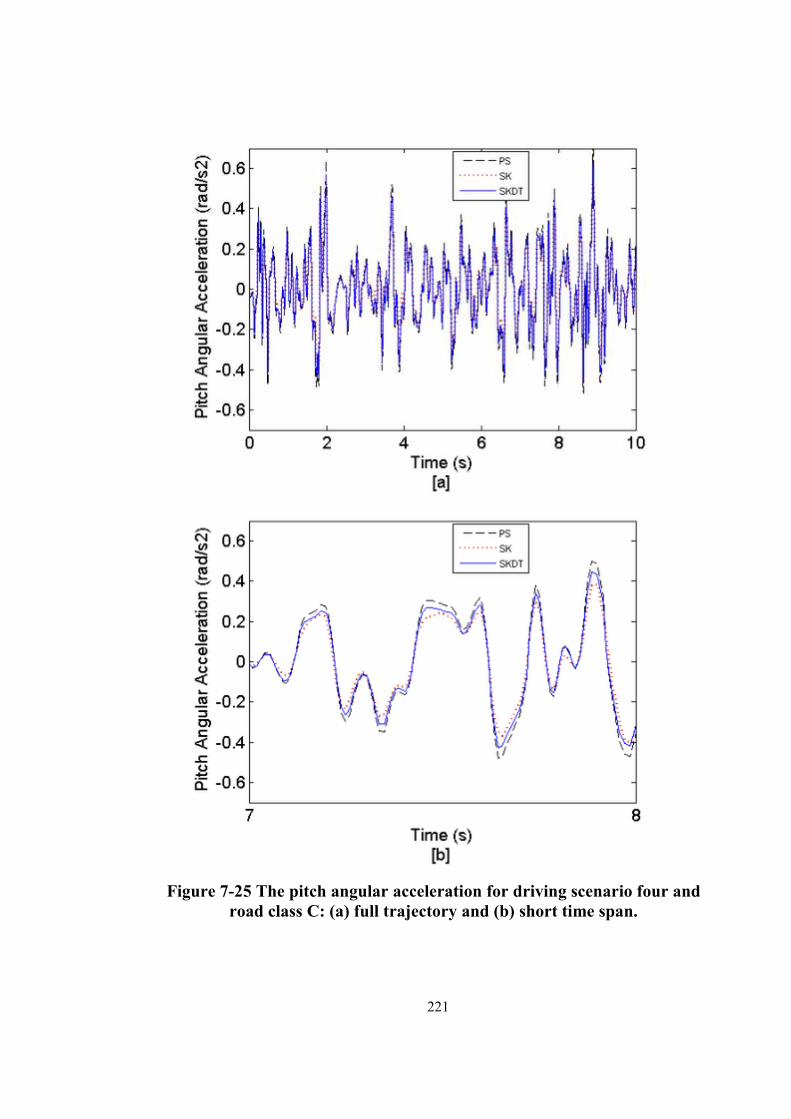
221
Figure 7-25 The pitch angular acceleration for driving scenario four and road class C: (a) full trajectory and (b) short time span.

222
Figure 7-26 The roll angular acceleration for driving scenario four and road class C: (a) full trajectory and (b) short time span.

223
Figure 7-27 The lateral acceleration for driving scenario four and road class C: (a) full trajectory and (b) short time span.

224
Figure 7-28 The vehicle sprung mass m3‘s vertical displacement for driving scenario four and road class C: (a) full trajectory and (b) short time span.

225
Figure 7-29 The rollover threshold in driving scenario four and road class C: (a) full trajectory and (b) short time span.

226
Compared to the passive suspension system, the normalized RMS body
vertical acceleration (NV) of the SK and SKDT suspension systems have
decreased by 14.21% and 17.67% respectively as shown in Figure 7-30. The
normalized RMS pitch angular accelerations (NP) of the SK and SKDT
suspension systems decreased by 12.27% and 10.88% respectively (Figure 7-31).
However Figure 7-32 shows that the normalized RMS roll angular
acceleration (NR) of the SK and SKDT systems have increased by 0.34% and
10%. Compared to the PS system, the NL (Normalized Lateral acceleration) of
the SK and SKDT suspension systems have decreased by 5.26% and 9%
respectively (Figure 7-33 ). As shown in Figure 7-34., the road handling
performance of the SK and SKDT systems have decreased by only 2.66% and
2% compared to the passive suspension system which is within the acceptable
range. Hence, the SK and SKDT suspension controllers can effectively improve
vehicle ride comfort while the vehicle is moving on road class C.
Figure 7-30 Vehicle body vertical acceleration comparison.

227
Figure 7-31 Vehicle body pitch angular acceleration comparison.
Figure 7-32 Vehicle body roll angular acceleration comparison.

228
Figure 7-33 Vehicle body lateral acceleration comparison.
Figure 7-34. Vehicle road handling performance comparison.

229
7.5 Conclusions
This chapter described the conclusions reached from the experimental analysis of
the full car model along with the Quanser quarter-car suspension plant that were
carried out to investigate the proposed skyhook control suspension system and
the Direct Tilt Control system. The vehicle performance analysis using the
Quanser quarter-car suspension plant at the front left and rear right wheel of the
full car model was presented separately in two different sections. It has been
observed that the results of the two environments are slightly different. The
reason is the distances from C.G. to the front and rear wheels are different for the
full car model.
The SK and SKDT control systems were applied to the dynamic model of
the full car. It takes the road bank angle into consideration to evaluate the
performances of the controllers. The behaviour of the vehicle body vertical
acceleration, pitch angular acceleration and roll angular acceleration were
evaluated in the frequency domain. While travelling on all the road profiles, it
has been ascertained that, the vehicle body vertical acceleration and pitch angular
acceleration of both the SK and SKDT systems remained closer to 0 db than the
PS system at a wide range of frequencies, especially at frequencies where
humans are more sensitive to vibrations.
Time domain analysis was also carried out to investigate the performance
of the systems. NV (Normalize body vertical acceleration) and NP (Normalized
pitch angular acceleration) have been calculated and it has been found that both
the SK and SKDT systems significantly reduced the vehicle body vertical
acceleration and pitch angular acceleration in all instances compared to the PS
system. However the normalized RMS of the roll angular acceleration (NR) of
the SKDT system increased significantly with the tilting action. Fortunately, the
vehicle’s roll angular acceleration only accounts for less than 20% of vehicle ride

230
comfort, in terms of ride comfort index specified by ISO 2631-1 standard. Hence
the vehicle ride comfort would not be affected significantly by the large roll
angular acceleration. Moreover, the appropriate tilting action reduced the lateral
acceleration experienced by passengers and improved the vehicle ride comfort, as
the NL (Normalized Lateral acceleration) of the SK and SKDT suspension
systems have decreased compared to the PS system. The road handling
performance of both suspension systems has also been evaluated and it has been
found that the performance decreased slightly compared to the passive
suspension system which is within the acceptable range. The stability of the
resulting closed loop system was then investigated.
The response of the vehicle’s desired tilting angle (faiD) for the
corresponding steering input signal (Delta) and the road bank angle (β) have been
shown. The required actuator force to tilt the vehicle according to the desired
tilting angle was also been observed. Overall it has been realized that the
proposed skyhook control system on its own can improve the vehicle ride
comfort keeping the road handling performance within an acceptable range. The
SKDT system shows that this control strategy is capable of tilting a vehicle
inward which would act against the lateral acceleration result of the steering
manoeuvres. The designed SKDT system was capable of maintaining the
system’s tilt state by keeping the vehicle stable and safe from rollover.

231
Chapter 8
Conclusions and recommendations
8.1 Introduction
This thesis began by considering two key elements as the main objectives of this
research project. The first goal was to develop a semi-active control strategy that
would reduce the unwanted effects of various road conditions and driving
manoeuvres on the vehicle body and the passengers. The second objective was to
design and study the performance of a semi-active suspension system suitable for
the standard passenger vehicle and to improve the cornering performance of the
vehicle.
In this thesis, various types of semi-active control approaches for vehicle
suspension systems have been studied. A new modified skyhook control strategy
with adaptive skyhook gain has been presented which is claimed as a novel idea
by the reviewers in the International Journal of Vehicle Mechanics and Mobility
titled, “Vehicle System Dynamics”.
An extensive literature review has been done on both academic research
and industrial advancement of vehicle tilting technology to improve cornering
performance. But to date, none of them considered the road bank angle in the
control system design and the modelling of the dynamic model of the standard
passenger tilting vehicles. This study designed and developed a new analytical
full vehicle model incorporating the road bank angle in the vehicle dynamics. A
direct tilt control method along with the proposed modified skyhook controlled
closed loop feedback system was developed to control the tilt action of the
vehicle. This system improved the performance of the vehicle during cornering
with little or no skidding. This was achieved by using a new approach of tilting

232
the standard passenger vehicle inward during cornering considering the road
bank angle along with the steering angle, lateral position acceleration, yaw rate
and velocity of the vehicle.
8.2 Overview of the study
After a brief introduction on automotive suspension systems in the first chapter,
an extensive literature review was done on many robust and optimal control
approaches or algorithms. This included linear time invariant H-infinity control
(LTIH), linear parameter varying control (LPV) and model-predictive controls
(MPC). Five widely known control approaches were reviewed more deeply,
namely the Linear quadratic regulator & Linear Quadratic Gaussian, sliding
mode control, Fuzzy and neuro-fuzzy control, sky-hook and ground-hook
approaches. It was found that the skyhook control strategy is the most widely
used among all other control strategies due to its simplicity for practical
implementation. But still there is a great scope of work to be done to modify the
skyhook control strategy to achieve better performance. Different types of
damper technologies have been also discussed in this thesis and it has been
ascertained that the linear electromagnetic damper is best for the semi-active
suspension system due to its fast response time which is better than the best
hydraulic device. A brief literature review on automotive tilting technology was
done in this thesis which suggests that a direct tilting method needs to be
developed to tilt the standard passenger vehicle inward during cornering
considering the road bank angle.
The vehicle suspension system has been categorised and discussed briefly.
It has been explained that the semi-active suspension system is the most suitable
for investigation in this research. A brief description of the quarter-car model has
been given as well as an explanation of the motion equations used in the model.
The high and low bandwidth suspension system has also been discussed. As
there is no requirement for a static load force in this research, a two degree of

233
freedom HBC semi-active suspension system was used to investigate different
semi-active control algorithms in this thesis. An extensive comparison of quarter-
car models extracted from the study of various researchers has been presented.
A brief discussion on a proposed modified skyhook control approach, the
optimal skyhook control of Nguyen et al. [51], modified skyhook control of
Bessinger et al. [15] and continuous skyhook control of Karnopp et al. [14] was
presented. A road profile has been generated to study the performance of the
different controllers. The two degree of freedom quarter-car model has been
simulated to compare the controllers’ performances. The Quanser quarter-car
suspension plant has been also used to compare the performance of the
controllers in an experimental environment. From the above simulation and
experimental analysis, it can be concluded that the proposed modified skyhook
controlled closed loop feedback system provides the best performance of those
investigated because it decreases sprung mass acceleration to a large extent
compared to the passive system and other skyhook controllers described in the
literature. It also keeps road handling performance within the acceptable range.
These models have also been evaluated in terms of human vibration perception
and admissible acceleration levels based on ISO 2631.
This thesis also presents a methodology on how to integrate the proposed
skyhook control in a full car model to improve ride comfort and handling via a
semi-active suspension system. It demonstrates the direct tilt control strategy
which can tilt a vehicle inwards to act against the roll movement due to steering
manoeuvres as well as road bank angle. A technique to determine the vehicle
rollover propensity has also been described. The road profile and four driving
scenarios have also been briefly discussed in this chapter which forms a basis for
the analysis described in the next following chapters. To compare and evaluate
the results of the simulation environment and experimental setup, three criteria

234
have been set. The ride comfort of the vehicle will be evaluated by comparing the
results of the normalized RMS value of vehicle body vertical acceleration,
vehicle pitch angular acceleration, roll angular acceleration and lateral
acceleration. Evaluation of road handling performance will be done by
comparing the tyre forces normalized to the static forces that acts on the vehicle’s
wheels.
The SK and SKDT systems were applied to the dynamic model of a full
car which considers the road bank angle. At first, the responses of the dynamic
model of the full car on different road class A, B and C defined by ISO8608 and
also a combined road profile have been observed. In this section, PS and SK
systems were analyzed separately. The behaviour of the vehicle body vertical
acceleration and pitch angular acceleration were examined in the frequency
domain. While travelling on all the road profiles, it has been ascertained that, the
vehicle body vertical acceleration and pitch angular acceleration of the SK
system remain closer to 0 db than the PS system at a wide range of frequencies,
particularly in the region where humans are more sensitive to vibrations.
The time domain analysis was also carried out on the full car model using
the PS and the SK system separately. In this sub-section, vertical displacement of
the vehicle front left sprung mass m1, vehicle body vertical acceleration and pitch
angular acceleration have been assessed. NV (Normalize body vertical
acceleration) and NP (Normalized pitch angular acceleration) have also been
calculated and it has been found that the SK system significantly reduced the
vehicle body vertical acceleration and pitch angular acceleration in all instances
compared to the PS system. However the road handling performance of the SK
controlled suspension system decreased slightly compared to the passive
suspension system. But the SK system’s weighted RMS acceleration value of the
sprung mass obtained in this simulation was always within the acceptable range

235
of international code ISO 2631 [143]. Since the vehicle was traversing on a
straight road, the differences in roll angular and lateral acceleration of both
systems were negligible in this analysis.
Subsequently, the simulations of the dynamic model of a full car with
different driving scenarios (described in Section (5.4)) was carried out using the
SKDT system. Vehicle reaction to the driving scenarios of both the PS and the
SKDT semi-active suspension systems have been described in this section. The
response of the vehicle’s desired tilting angle (faiD) for the corresponding
steering input signal (Delta) and the road bank angle (β) have been shown. The
required actuator force to tilt the vehicle according to the desired tilting angle
was also observed.
Here the time domain responses of the vertical displacement of the vehicle
front left sprung mass m1, vehicle body vertical, pitch angular, roll angular and
lateral acceleration for each driving scenario have been shown and it was quite
evident that the displacement of sprung mass m1, the vehicle vertical, pitch
angular accelerations and the lateral acceleration of the SKDT system have
decreased compared to the PS system. Compared to the passive suspension
system, the NV and NP of the SKDT suspension system have decreased
significantly. However the normalized RMS of the roll angular acceleration (NR)
of the SKDT system was increased significantly for the tilting action.
Fortunately, the roll angular acceleration of vehicle only accounts for less than
20% of vehicle ride comfort, in terms of ride comfort index specified by the ISO
2631-1 standard. Hence vehicle ride comfort would not be affected significantly
by the large roll angular acceleration. Moreover, the appropriate tilting action
reduces the lateral acceleration experienced by passengers and improved the
vehicle ride comfort, as the NL (Normalized Lateral acceleration) of the SKDT

236
suspension system was decreased by 10.01% compared to the PS system. The
stability of the resulting closed loop system was then investigated.
Road class C and driving scenario four were used to evaluate the
performance of the PS, SK and SKDT systems. It has been realized that the
proposed skyhook controlled closed loop feedback system on its own can
improve vehicle ride comfort keeping the road handling performance within an
acceptable range. The SKDT system shows that this control strategy is capable of
tilting a vehicle inward which would act against the lateral acceleration result of
the steering manoeuvres. The designed SKDT system was capable of maintaining
the system’s tilt state by keeping the vehicle stable and safe from rollover. This
research has indicated the potential of the SKDT suspension system in improving
cornering performances of the vehicle and paves the way of a future work on a
vehicle’s integrated system for chassis control.
The vehicle performance analysis using the Quanser quarter-car
suspension plant at front left and rear right wheel of the full car model is
presented separately in two different sections. It has been observed that the
results of the two environments are slightly different. The reason is the distances
from C.G. to the front and rear wheel are different for the full car model.
The SK and SKDT control systems were applied to the dynamic model of
the full car model which considers the road bank angle to evaluate the
performances of the controllers. The behaviour of the vehicle body vertical
acceleration, pitch angular acceleration and roll angular acceleration were
examined in the frequency domain. While travelling on all the road profiles, it
has been ascertained that, the vehicle body vertical acceleration and pitch angular
acceleration of both the SK and SKDT systems remained closer to 0 db than the

237
PS system at a wide range of frequencies, particularly in the region where
humans are more sensitive to vibrations.
The time domain analysis was also carried out to investigate the
performance of the systems. NV (Normalize body vertical acceleration) and NP
(Normalized pitch angular acceleration) have also been calculated and it has been
found that both the SK and SKDT system significantly reduced the vehicle body
vertical acceleration and pitch angular acceleration in all instances compared to
the PS system. However the normalized RMS of the roll angular acceleration
(NR) of the SKDT system increased significantly for the tilting action.
Fortunately, the roll angular acceleration of vehicle only accounts for less than
20% of vehicle ride comfort, in terms of ride comfort index specified by the ISO
2631-1 standard. Hence the vehicle ride comfort would not be affected
significantly by the large roll angular acceleration. Moreover, the appropriate
tilting action reduces the lateral acceleration experienced by passengers and
improved the vehicle ride comfort, as the NL (Normalized Lateral acceleration)
of the SK and SKDT suspension system decreased compared to the PS system.
The road handling performances of both suspension systems have also been
evaluated and it has been found that the performance decreased slightly
compared to the passive suspension system which is within the acceptable range.
The stability of the resulting closed loop system was then investigated.
The response of the vehicle’s desired tilting angle (faiD) for the
corresponding steering input signal (Delta) and the road bank angle (β) have been
shown. The required actuator force to tilt the vehicle according to the desired
tilting angle had also been observed. Overall it has been realized that the
proposed skyhook control system on its own can improve the vehicle ride
comfort keeping the road handling performance within an acceptable range. The
SKDT system shows that this control strategy is capable of tilting a vehicle
238
inward which would act against the lateral acceleration resulting from the
steering manoeuvres. The designed SKDT system was capable of maintaining the
system’s tilt state by keeping the vehicle stable and safe from rollover.
This thesis presents a novel idea on how to integrate vehicle ride comfort
and handling control via semi-active suspensions. It demonstrated that the
integrated suspension control strategy can tilt a vehicle inwards to act against the
roll moment due to steering manoeuvres.
8.3 Recommendations for future study
This research has indicated the potential of the SKDT suspension system in
improving cornering performances of the vehicle and paves the way for future
work on vehicle’s integrated system for chassis control. Based on my completed
research work on semi-active dampers and semi-active controlled suspension
systems, the following research is recommended for further study.
Development of a microcontroller for the proposed modified skyhook
controlled closed loop feedback system and the direct tilt control method is an
important aspect of future work. Theoretical and experimental studies of the
control methods have already been done.
Development of a commercial semi-active suspension system with linear
electromagnetic damper would be a potential work.
Real-time testing of the developed damper control strategies on an actual
standard passenger vehicle suspension system and testing on standard test tracks
is recommended. Comparing the real-time test results with the results obtained
through numerical simulation using CarSim or Adams/Car would be beneficial as
well.

239
References
[1] web8. (August, 2012). www.port.ac.uk. [2] Y. Chen, "Skyhook surface sliding mode control on semi-active vehicle
suspension systems for ride comfort enhancement," Engineering, vol. 1, pp. 23-32, 2009.
[3] W. Gao, et al., "A stochastic quarter-car model for dynamic analysis of vehicles with uncertain parameters," Vehicle System Dynamics: International Journal of Vehicle Mechanics and Mobility, vol. 46, pp. 1159 - 1169, 2008.
[4] S. B. Choi, et al., "H-infinity control performance of a full-vehicle suspension featuring magnetorheological dampers," Vehicle System Dynamics vol. 38(5), pp. 341-360, 2002.
[5] M. Ahmadian and D. E. Simon, "An analytical and experimental evaluation of magneto rheological suspensions for heavy trucks," Vehicle System Dynamics, vol. 37, pp. 38-49, 2003.
[6] M. Ahmadian and N. Vahdati, "Transient dynamics of semiactive suspensions with hybrid control," Journal of intelligent material systems and structures, vol. 17, pp. 145-153, 2006.
[7] N. Yagiz and L. E. Sakman, "Robust sliding mode control of a full vehicle without suspension gap loss," Journal of Vibration and Control, vol. 11(11), pp. 1357-1374 2005.
[8] M. Yu, et al., "Study on MR semi-active suspension system and its road testing," Journal of intelligent material systems and structures, vol. 17, pp. 801-806, 2006.
[9] N. Eslaminasab, et al., "A neural network based fuzzy control approach to improve ride comfort and road handling of heavy vehicles using semi-active dampers," International Journal of Heavy Vehicle Systems, vol. 14, pp. 135-157, 2007.
[10] S. Choi, et al., "A hysteresis model for the field-dependent damping force of a magnetorheological damper," Journal of Sound and Vibration, vol. 245, p. 375, 2001.
[11] K. G. Sung, et al., "Discrete-time fuzzy sliding mode control for a vehicle suspension system featuring an electrorheological fluid damper," Smart materials and structures, vol. 16, p. 798, 2007.
[12] X. Fang and W. Chen, "Fuzzy control technology and the application to vehicle semi-active suspension," Chinese journal of Mechanical Engineering, vol. 35, pp. 98-100, 1999.
[13] X. Dong, et al., "Adaptive Fuzzy Neural Network Control for Transient Dynamics of Magneto-rheological Suspension with Time-Delay," Advances in Neural Networks-ISNN pp. 1046-1051, 2006.
[14] J. Yang, et al., "Adaptive fuzzy control of lateral semi-active suspension for high-speed railway vehicle," Computational Intelligence, pp. 1104-1115, (2006.
[15] D. Karnopp, et al., "Vibration control using semi-active force generators," Journal of Engineering for Industry, vol. 96, pp. 619-626, 1974.
[16] F. Besinger, et al., "Force control of a semi-active damper," Vehicle System Dynamics, vol. 24, pp. 695-723, 1995.

240
[17] L. H. Nguyen, et al., "Modified skyhook control of a suspension system with hydraulic strut mount," in ICCAS-SICE 2009 - ICROS-SICE International Joint Conference 2009, Proceedings, 2009, pp. 1347-1352.
[18] R. Marino, et al., "Nonlinear PI front and rear steering control in four wheel steering vehicles," Vehicle system dynamics, vol. 45, pp. 1149-1168, 2007.
[19] B. Li and F. Yu, "Optimal model following control of four-wheel active steering vehicle," 2009, pp. 881-886.
[20] F. Du, et al., "Robust Control Study for Four-Wheel Active Steering Vehicle," in International Conference on Electrical and Control Engineering, ICECE,, 2010, pp. 1830-1833.
[21] R. Goodall, "Tilting trains and beyond-the future for active railway suspensions. 1. improving passenger comfort," Computing & Control Engineering Journal, vol. 10, pp. 153-160, 1999.
[22] R. Goodall, "Tilting trains and beyond. The future for active railway suspensions. 2. Improving stability and guidance," Computing & Control Engineering Journal, vol. 10, pp. 221-230, 1999.
[23] web13. (August, 2012). http://www.dailymail.co.uk/sciencetech/article-1263509/Meet-electric-powered-Land-Glider-half-width-normal-car.html. Available: http://delphi.com/manufacturers/auto/other/ride/magneride/
[24] web9. (August, 2012). http://www.seriouswheels.com/cars/top-1997-Mercedes-Benz-F-300-Life-Jet-Concept.htm. Available: http://delphi.com/manufacturers/auto/other/ride/magneride/
[25] web11. (August, 2012). http://www.carver-engineering.com/. Available: http://delphi.com/manufacturers/auto/other/ride/magneride/
[26] D. Karnopp and R. Hibbard, "Optimum roll angle behavior for tilting ground vehicles," ASME DYN SYST CONTROL DIV PUBL DSC, ASME, NEW YORK, NY(USA), 1992, vol. 44, pp. 29-37, 1992.
[27] R. Hibbard and D. Karnopp, "Twenty first century transportation system solutions-A new type of small, relatively tall and narrow active tilting commuter vehicle," Vehicle system dynamics, vol. 25, pp. 321-347, 1996.
[28] S. G. So and D. Karnopp, "Methods of controlling the lean angle of tilting vehicles," DSC, vol. 52, pp. 311-319, 1993.
[29] A. Saccon, et al., "A virtual rider for motorcycles: An approach based on optimal control and maneuver regulation," 2008, pp. 243-248.
[30] R. Frezza and A. Beghi, "Simulating a motorcycle driver," New trends in Nonlinear Dynamics and Control and their Applications, pp. 175-186, 2003.
[31] S. Kidane, et al., "Road bank angle considerations in modeling and tilt stability controller design for narrow commuter vehicles," in Proceedings of the American Control Conference, Minneapolis, Minnesota, USA, 2006, p. 6.
[32] D. Piyabongkarn, et al., "Active direct tilt control for stability enhancement of a narrow commuter vehicle," International Journal of Automotive Technology, vol. 5, pp. 77-88, 2004.
[33] J. Wang and S. Shen, "Integrated vehicle ride and roll control via active suspensions," Vehicle System Dynamics, vol. 46, pp. 495-508, 2008.
[34] W. Jones, "Easy ride: Bose Corp. uses speaker technology to give cars adaptive suspension," Spectrum, IEEE, vol. 42, pp. 12-14, 2005.
[35] web28, "http://www.motortrend.com/auto_shows/tokyo/2009/," August, 2012.

241
[36] J. B. Gohl, "Narrow Tilting Vehicles: Modeling and Steering Based, Tilt Control," University of Minnesota, 2003.
[37] R. Rajamani, et al., "Dynamics of narrow tilting vehicles," Mathematical and Computer modelling of dynamical systems, vol. 9, pp. 209-231, 2003.
[38] S. G. So and D. Karnopp, "Switching strategies for narrow ground vehicles with dual mode automatic tilt control," International journal of vehicle design, vol. 18, pp. 518-32, 1997.
[39] S. Sang-Gyun and D. Karnopp, "Switching strategies for narrow ground vehicles with dual mode automatic tilt control," International journal of vehicle design, vol. 18, pp. 518-32, 1997.
[40] Y. Li, et al., "An active roll mode suspension system for ground vehicles," Journal of Basic Engineering, vol. 90, p. 167, 1968.
[41] L. Mourad, et al., "A Lateral Control Strategy for Narrow Tilting Commuter Vehicle Based on the Perceived Lateral Acceleration," in 18th IFAC World Congress Milano (Italy), September 2011, pp. 6254-6259.
[42] N. Roqueiro, et al., "Sliding Mode Controller and Flatness Based Set-Point Generator for a Three Wheeled Narrow Vehicle," in 18th IFAC World Congress Milano (Italy), September, 2011, pp. 11925-11930.
[43] N. Amati, et al., "Dynamic modelling and experimental validation of three wheeled tilting vehicles," Vehicle system dynamics, vol. 49, pp. 889-914, July, 2012.
[44] J. Edelmann, et al., "Modelling and analysis of the dynamics of a tilting three-wheeled vehicle," Multibody System Dynamics, pp. 1-19, 2011.
[45] X. Jiang, et al., "Semi-active control of a vehicle suspension using magneto-rheological damper," Journal of Central South University, vol. 19, pp. 1839-1845, 2012.
[46] S. Z. Chen, et al., "Magnetorheological Semi-Active Suspension Demonstration for Off-Road Vehicles," Advanced Science Letters, vol. 12, pp. 1-6, 2012.
[47] P. Sun, et al., "A New Kind of Semi-Active Suspension Magnetorheological Fluid Shock Absorber Damping Force Model," Advanced Materials Research, vol. 549, pp. 856-860, 2012.
[48] E. Pellegrini, et al., "A dynamic feedforward control approach for a semi-active damper based on a new hysteresis model," 2011, pp. 6248-6253.
[49] W. R. Wang, et al., "Analysis of Vane Hydraulic Damp Static Seal Mechanism and Performance Influencing Factors," Applied Mechanics and Materials, vol. 152, pp. 1774-1778, 2012.
[50] ISO, "Mechanical vibration-road surface profiles-reporting of measured data, TC 108/SC 2 (Mechanical vibration and shock/measurement and evaluation of mechanical vibration and shocks as applied to machines, vehicles and structures), ISO 8608: E Standards," ISO, 1995.
[51] Q. H. Nguyen and S. B. Choi, "Optimal design of MR shock absorber and application to vehicle suspension," Smart materials and structures, vol. 18, p. 035012, 2009.
[52] D. Karnopp, et al., "Vibration Control Using Semi-Active Force Generators," ASME Pap, 1973.
[53] D. Hrovat, "Survey of advanced suspension developments and related optimal control applications," Automatica, vol. 33, pp. 1781-1817, 1997.

242
[54] C. Poussot-Vassal, et al., "A new semi-active suspension control strategy through LPV technique," Control Engineering Practice, vol. 16, pp. 1519-1534, 2008.
[55] C. Rossi and G. Lucente, "H∞ control of automotive semi-active suspensions," in In Proceedings of the 1st IFAC symposium on advances in automotive control Salerno, Italy, 2004.
[56] A. Zin, et al., "Switched H∞ control strategy of automotive active suspensions," in In Proceedings of the 16th IFAC world congress (WC), Praha, Czech Republic, 2005.
[57] N. Giorgetti, et al., "Hybrid model predictive control application towards optimal semi-active suspension," International Journal of Control, vol. 79, pp. 521-533, 2006.
[58] C. Poussot-Vassal, et al., "A self tuning LPV/H∞ suspension controller for a multi-body quarter vehicle model," in In Proceedings of the 10th mini-conference on vehicle system dynamics, identification and anomalies (VSDIA), Budapest, Hungary, 2007.
[59] P. Gaspar, et al., "Active suspension design using LPV control," in In Proceedings of the 1st IFAC symposium on advances in automotive control (AAC), (pp. 584–589), Salerno, Italy., 2004.
[60] A. Zin, et al., "Robust LPV–∞ control for active suspensions with performance adaptation in view of global chassis control," Vehicle System Dynamics, vol. 46, pp. 889-912, 2008.
[61] M. Canale, et al., "Semi-Active Suspension Control Using &# 8220; Fast&# 8221; Model-Predictive Techniques," Control Systems Technology, IEEE Transactions on, vol. 14, pp. 1034-1046, 2006.
[62] A. Giua, et al., "Design of a predictive semiactive suspension system," Vehicle System Dynamics, vol. 41, pp. 277-300, 2004.
[63] S. F. Choudhury and D. M. A. R. Sarkar, "An approach on performance comparison between automotive passive suspension and active suspension system (pid controller) using matlab/simulink," Journal of Theoretical and Applied Information Technology, vol. 43, pp. 295-300, 2012.
[64] M. M. ElMadany and Z. S. Abduljabbar, "Linear quadratic Gaussian control of a quarter-car suspension," Vehicle System Dynamics, vol. 32, pp. 479-497, 1999.
[65] R. Krtolica and D. Hrovat, "Optimal active suspension control based on a half-car model: An analytical solution," Automatic Control, IEEE Transactions on, vol. 37, pp. 528-532, 1992.
[66] D. Hrovat, "Optimal active suspensions for 3D vehicle models," in Proceedings of American control conference, 1991, pp. 1534-1541.
[67] J. Doyle and G. Stein, "Multivariable feedback design: Concepts for a classical/modern synthesis," Automatic Control, IEEE Transactions on, vol. 26, pp. 4-16, 1981.
[68] C. R. Fuller, et al., Active control of vibration. London, UK: Academic Press, 1997.
[69] D. Hrovat, "Applications of optimal control to advanced automotive suspension design," Journal of dynamic systems, measurement, and control, vol. 115, p. 328, 1993.

243
[70] R. Shisheie, et al., "Linear Quadratic Regulator Time-Delay Controller for Hydraulic Actuator," Journal of Basic and Applied Scientific Research, 2012.
[71] G. Prokop and R. Sharp, "Performance enhancement of limited-bandwidth active automotive suspensions by road preview," in IEEE Proceedings-Control Theory and Applications, 1995, pp. 140-148.
[72] Y. Shen, "Vehicle suspension vibration control with magnetorheological dampers," PhD. Thesis, University of Waterloo, 2005.
[73] G. Foo and M. Rahman, "Sensorless sliding-mode MTPA control of an IPM synchronous motor drive using a sliding-mode observer and HF signal injection," Industrial Electronics, IEEE Transactions on, vol. 57, pp. 1270-1278, 2010.
[74] R. Gupta, et al., "Multiband hysteresis modulation and switching characterization for sliding-mode-controlled cascaded multilevel inverter," Industrial Electronics, IEEE Transactions on, vol. 57, pp. 2344-2353, 2010.
[75] P. Shi, et al., "On designing of sliding-mode control for stochastic jump systems," Automatic Control, IEEE Transactions on, vol. 51, pp. 97-103, 2006.
[76] A. Shiri, "Robust Sliding Mode Control of Electromagnetic Suspension System with Parameter Uncertainty," Journal of Applied Sciences, Engineering and Technology, vol. 10, pp. 1677-1683, 2012.
[77] T. Orowska-Kowalska, et al., "Implementation of a sliding-mode controller with an integral function and fuzzy gain value for the electrical drive with an elastic joint," Industrial Electronics, IEEE Transactions on, vol. 57, pp. 1309-1317, 2010.
[78] L. Huang and X. Mao, "SMC design for robust H [infinity] control of uncertain stochastic delay systems," Automatica, vol. 46, pp. 405-412, 2010.
[79] L. Wu and D. W. C. Ho, "Sliding mode control of singular stochastic hybrid systems," Automatica, vol. 46, pp. 779-783, 2010.
[80] H. H. Choi, "LMI-based sliding surface design for integral sliding mode control of mismatched uncertain systems," Automatic Control, IEEE Transactions on, vol. 52, pp. 736-742, 2007.
[81] Y. W. Tsai, et al., "Sliding mode control for unmatched uncertain systems with totally invariant property and exponential stability," Journal of the Chinese Institute of Engineers, vol. 29, pp. 179-183, 2006.
[82] M. L. Chan, et al., "Sliding mode controller for linear systems with mismatched time-varying uncertainties," Journal of the Franklin Institute, vol. 337, pp. 105-115, 2000.
[83] N. Yagiz, et al., "Robust control of active suspensions for a full vehicle model using sliding mode control," JSME international journal. Series C, Mechanical systems, machine elements and manufacturing, vol. 43, pp. 253-258, 2000.
[84] A. Chamseddine, et al., "Control of linear full vehicle active suspension system using sliding mode techniques," 2006, pp. 1306-1311.
[85] N. Al-Holou, et al., "The development of fuzzy logic based controller for semi-active suspension system," 1994, pp. 1373-1376 vol. 2.
[86] A. J. Barr and J. Ray, "Control of an active suspension using fuzzy logic," in Proceedings of the Fifth IEEE International Conference on Fuzzy Systems, 1996, pp. 42-48 vol. 1.

244
[87] B. Yan, et al., "Design and test of a novel isolator with negative resistance electromagnetic shunt damping," Smart Materials and Structures, vol. 21, p. 035003, 2012.
[88] K. H. Youssef, et al., "Adaptive fuzzy APSO based inverse tracking-controller with an application to DC motors," Expert Systems with applications, vol. 36, pp. 3454-3458, 2009.
[89] H. Khalid, et al., "A PSO-trained adaptive neuro-fuzzy inference system for fault classification," in International Conference on Neural Computation, ICNC Valencia, Spain, 2010.
[90] R. Kashani and J. E. Strelow, "Fuzzy logic active and semi-active control of off-road vehicle suspensions," Vehicle system dynamics, vol. 32, pp. 409-420, 1999.
[91] Y. Shen, et al., "Semi-active vibration control schemes for suspension systems using magnetorheological dampers," Journal of Vibration and Control, vol. 12, pp. 3-24, 2006.
[92] D. Karnopp, "Active damping in road vehicle suspension systems," Vehicle system dynamics, vol. 12, pp. 291-311, 1983.
[93] H. Li and R. M. Goodall, "Linear and non-linear skyhook damping control laws for active railway suspensions," Control Engineering Practice, vol. 7, pp. 843-850, 1999.
[94] D. L. M. Professor, "Semi-active control of wheel hop in ground vehicles," Vehicle system dynamics, vol. 12, pp. 317-330, 1983.
[95] S. M. Savaresi, et al., "Acceleration-Driven-Damper (ADD): An optimal control algorithm for comfort-oriented semiactive suspensions," Journal of dynamic systems, measurement, and control, vol. 127, p. 218, 2005.
[96] S. M. Savaresi and C. Spelta, "Mixed sky-hook and ADD: Approaching the filtering limits of a semi-active suspension," Journal of dynamic systems, measurement, and control, vol. 129, p. 382, 2007.
[97] S. A. A. Bakar, et al., "Vehicle ride performance with semi-active suspension system using modified skyhook algorithm and current generator model," International Journal of Vehicle Autonomous Systems, vol. 6, pp. 197-221, 2008.
[98] L. R. Miller and C. M. Nobles, "Methods for eliminating jerk and noise in semi-active suspensions," presented at the SAE 1990 Transactions, 1990.
[99] R. T. Tong, Ride control: a two-state design for heavy vehicle suspension: University of Illinois at Chicago, 2001.
[100] A. M. A. Soliman, et al., "Fuzzy-Skyhook Control for Active Suspension Systems Applied to a Full Vehicle Model," International Journal of Engineering and Technology, vol. 2, pp. 01-12, 2012.
[101] A. S. M. S. Islam and A. Ahmed, "Comparative performance study of magneto-rheological fluid based damper for vehicle suspension," in Proceedings of the International Conference on Mechanical Engineering, 2005.
[102] S. B. A. Kashem, et al., "Comparison between different sets of suspension parameters and introduction of new modified skyhook control strategy incorporating varying road condition," Vehicle system dynamics, vol. 50, pp. 1173-1190, 2012.
[103] M. Valasek, et al., "Development of semi-active road-friendly truck suspensions," Control Engineering Practice, vol. 6, pp. 735-744, 1998.

245
[104] K. Yi, et al., Dynamic tire force control by semi-active suspensions: University of California Transportation Center, University of California, 1992.
[105] M. Valášek, et al., "Extended ground-hook-new concept of semi-active control of truck's suspension," Vehicle system dynamics, vol. 27, pp. 289-303, 1997.
[106] web7. (August, 2012). http://www.conceptcarz.com/vehicle/z11633/Carver-One.aspx. [107] web16. (August, 2012). http://lynk.ly/stories/view/1479328. Available:
http://delphi.com/manufacturers/auto/other/ride/magneride/ [108] web17. (August, 2012). http://www.i4u.com/9754/carver-one-first-tilting-three-
wheeler-market. Available: http://delphi.com/manufacturers/auto/other/ride/magneride/
[109] R. Rajamani, Vehicle dynamics and control: Springer Verlag, New York, . 2006. [110] web14. (August, 2012). http://www.bmwblog.com/2009/10/09/bmw-unveils-
clever-concept/. [111] web12. (August, 2012). http://www.MP3.piaggio.com/. Available:
http://delphi.com/manufacturers/auto/other/ride/magneride/ [112] A. Snell, "An active roll-moment control strategy for narrow tilting commuter
vehicles," Vehicle system dynamics, vol. 29, pp. 277-307, 1998. [113] A. Poelgeest, et al., "Development of a Steer Tilt Controller for a Three
Wheeled Tilting Vehicle," Proceedings of the ASME International Mechanical Engineering Congress and Exposition, IMECE, Seattle, USA, 2007.
[114] S. Kidane, et al., "A fundamental investigation of tilt control systems for narrow commuter vehicles," Vehicle system dynamics, vol. 46, pp. 295-322, 2008.
[115] J. Chiou, et al., "Tilting motion control in narrow tilting vehicle using double-loop PID controller," in Proceedings of the 7th Asian Control Conference, 978-89-956056-1/09, 2009, pp. 913-918.
[116] M. Defoort and T. Murakami, "Sliding-mode control scheme for an intelligent bicycle," Industrial Electronics, IEEE Transactions on, vol. 56, pp. 3357-3368, 2009.
[117] U. Nenner, et al., "Robust stabilization of an unmanned motorcycle," in Robotics, Automation and Mechatronics, IEEE Conference on, Chengdu, China, 2008, pp. 101-106.
[118] web19. (August, 2012). http://driftjapan.com/blog/car-parts/drift-car-suspension/. Available: http://delphi.com/manufacturers/auto/other/ride/magneride/
[119] Y. Suda, et al., "Study on electromagnetic damper for automobiles with nonlinear damping force characteristics:(Road test and theoretical analysis)," Vehicle System Dynamics, vol. 41, pp. 637-646, 2004.
[120] T. Gillespie, "Development of semi-active damper for heavy off-road military vehicles," 2006.
[121] S. Irmscher and E. Hees, "Experience in semi-active damping with state estimators," in proceeding of AVEC, 1966, pp. 193-206.
[122] D. Konik, et al., "Electronic damping control with continuously working damping valves (EDCC)—system description and functional requirements," in International Symposium on Advanced Vehicle Control, Aachen, Germany, 1996, pp. 87-104.
[123] T. Nakayama, et al., "Development of semi-active control system with PUDLIS," in In Proceedings of International Symposium on Advanced Vehicle Control, AVEC'96, Aachen University of Technology, 1996, pp. 233-239.

246
[124] K. Yi and B. S. Song, "A new adaptive sky-hook control of vehicle semi-active suspensions," Proceedings of the Institution of Mechanical Engineers, Part D: Journal of Automobile Engineering, vol. 213, pp. 293-303, 1999.
[125] V. Sankaranarayanan, et al., "Semiactive suspension control of a light commercial vehicle," Mechatronics, IEEE/ASME Transactions on, vol. 13, pp. 598-604, 2008.
[126] H. Zhang, et al., "Comparison between Skyhook and Minimax Control Strategies for Semi-active Suspension System," World Academy of Science, Engineering and Technology, pp. 624-627, 2009.
[127] M. O. Abdalla, et al., "Linear matrix inequality based control of vehicle active suspension system," Vehicle System Dynamics: International Journal of Vehicle Mechanics and Mobility, vol. 47, pp. 121 - 134, 2009.
[128] M. M. Fateh and S. S. Alavi, "Impedance control of an active suspension system," Mechatronics, vol. 19, pp. 134-140, 2009.
[129] A. Faheem, et al., "The suspension dynamic analysis for a quarter car model and half car model," presented at the 3rd BSME-ASME International Conference on Thermal Engineering, Dhaka, 20-22 December 2006.
[130] A. Gupta, et al., "Design of electromagnetic shock absorbers," International Journal of Mechanics and Materials in Design, vol. 3, pp. 285-291, 2006.
[131] D. Guo, et al., "Neural network control for a semi-active vehicle suspension with a magnetorheological damper," Journal of Vibration and Control, vol. 10, pp. 461-471, 2004.
[132] G. Priyandoko, et al., "Vehicle active suspension system using skyhook adaptive neuro active force control," Mechanical Systems and Signal Processing, vol. 23, pp. 855-868, 2009.
[133] F. Scheibe and M. C. Smith, "Analytical solutions for optimal ride comfort and tyre grip for passive vehicle suspensions," Vehicle System Dynamics: International Journal of Vehicle Mechanics and Mobility, vol. 47, pp. 1229-1252, 2009.
[134] A. Kruczek and A. Stribrsky, "A full-car model for active suspension - Some practical aspects," in Proceedings of the IEEE International Conference on Mechatronics 2004, ICM'04, 2004, pp. 41-45.
[135] Y. Jia-ling and Z. Jia-qiang, "Semi-active Suspension System Design for Quarter-car Model using Model Reference Sliding Mode Control," in IEEE International Conference onVehicular Electronics and Safety, ICVES 2006, pp. 398-402.
[136] L. V. V. Gopala Rao and S. Narayanan, "Sky-hook control of nonlinear quarter car model traversing rough road matching performance of LQR control," Journal of Sound and Vibration, vol. 323, pp. 515-529, 2009.
[137] H. Du, et al., "Parameter-dependent input-delayed control of uncertain vehicle suspensions," Journal of Sound and Vibration, vol. 317, pp. 537-556, 2008.
[138] K. Sung, et al., "Road test evaluation of vibration control performance of vehicle suspension featuring electrorheological shock absorbers," Proceedings of the Institution of Mechanical Engineers, Part D: Journal of Automobile Engineering, vol. 222, pp. 685-698, 2008.
[139] C. Collette and A. Preumont, "High frequency energy transfer in semi-active suspension," Journal of Sound and Vibration, vol. 329, pp. 4604-4616, 2010.

247
[140] A. Shamsi and N. Choupani, "Continuous and Discontinuous Shock Absorber Control through Skyhook Strategy in Semi-Active Suspension System (4DOF Model)," in Proceedings of World Academy of Science, Engineering and Technology, 2008, pp. 746-750.
[141] O. Taniguchi, Vibration Engineers’ Handbook,: Yokendo Press,Tokyo, 1976. [142] S. Abramov, et al., "Semi-active suspension system simulation using Simulink,"
International Journal of Engineering Systems Modelling and Simulation, vol. 1, pp. 101-114, 2009.
[143] ISO, "Mechanical Vibration and Shock: Evaluation of Human Exposure to Whole-body Vibration. Part 1, General Requirements: International Standard ISO 2631-1: (E)," ISO, 1997.
[144] "Faulhaber DC MOTOR Technical information, Faulhaber DC motor specs, Germany," 2011.
[145] S. Ikenaga, et al., "Active suspension control of ground vehicle based on a full-vehicle model," in Proceedings of the American Control Conference, 2000, pp. 4019-4024.
[146] S. Ikenaga, et al., "Active suspension control using a novel strut and active filtered feedback: Design and implementation," in IEEE Conference on Control Applications - Proceedings, 1999, pp. 1502-1508.
[147] S. Sang-Gyun and D. Karnopp, "Active dual mode tilt control for narrow ground vehicles," Vehicle system dynamics, vol. 27, pp. 19-36, 1997.
[148] R. W. Allen, et al., "Computer Simulation Analysis of Light Vehicle Lateral/Directional Dynamic Stability," SAE transactions, vol. 108, pp. 482-497, 1999.

248
Appendix A
Simulink model
Jz*ddsai=aFf-bFr
dsai
m*ddy
dsai*V*m
ddfai*m*h
Beta*m*g
dy
1ddy
skyhook damping2
VelocityDeltaabdy lateral velocitydsai yaw rateCalphaFCalphaR
Ff
Fr
Tires lateral forces
uv
uv
1/s
1/s
Ff
dy
dsai
ddy
Jz
Mt
-1
-1
11g
10CalphaR
9CalphaF
8b
7a
6h
5Mt
4ddfai
3Beta
2Delta
1Velocity
Figure Appendix A1. Determine lateral position acceleration.

249
a*dsai dy + a*dsai (dy + a*dsai)/V
Delta - (dy + a*dsai)/V 2Cf *(Delta - (dy + a*dsai)/V)
b*dsai -dy + b*dsai 2Cr *( (-dy + b*dsai)/V)
2Fr
1Ff
s2uv
MathFunction2
2Constant4
-1Constant2
2Constant1
8CalphaR
7CalphaF
6dsai yaw rate
5dy lateral velocity
4b
3a
2Delta
1Velocity
Figure Appendix A2. Determine the front and rear tires lateral forces.

250
Appendix B
Matlab Code for frequency domain analysis of full car model clc clear all close all load('C:\Users\s\Dropbox\Full car cornering 160512\roadprofileClassABC20sEach280512.mat') SpecifiedStopTime = 60; RoadSteerBank280512; gcs; set_param('RoadSteerBank280512', 'StopTime', 'SpecifiedStopTime'); sim('C:\Users\s\Dropbox\Full car cornering 160512\RoadSteerBank280512.mdl') % set_param('RoadSteerBank280512', 'SimulationCommand', 'start'); % pause(SpecifiedStopTime); % roadprofile = roadprofileClassA; % roadprofile = roadprofileClassB; roadprofile = roadprofileClassC; % roadprofile = roadprofileClassABC20sEach280512; %change simulation time of the full model = dsaiDes; % Delta = SteerZero; % Beta = BetaZero; % Delta = Steer1; % Beta = BetaZero; % % Delta = SteerZero; % Beta = Beta1; % % Delta = Steer1; % Beta = Beta1; % Delta = Steer2; Beta = Beta2; %% ***************************************** %% First of all, chane the stop time to 10 then %% *********************************************** full_carstabilizedcModelz1z2z3z4usedSfunc160512; gcs; set_param('full_carstabilizedcModelz1z2z3z4usedSfunc160512', 'StopTime', 'SpecifiedStopTime'); % set_param('full_carstabilizedcModelz1z2z3z4usedSfunc160512', 'SimulationCommand', 'start'); full_carstabilizedcModelz1z2z3z4usedSfunc160512skyhook; gcs; set_param('full_carstabilizedcModelz1z2z3z4usedSfunc160512skyhook', 'StopTime', 'SpecifiedStopTime'); % set_param('full_carstabilizedcModelz1z2z3z4usedSfunc160512skyhook', 'SimulationCommand', 'start');

251
full_carstabilizedcModelz1z2z3z4usedSfunc160512DTC; gcs; set_param('full_carstabilizedcModelz1z2z3z4usedSfunc160512DTC', 'StopTime', 'SpecifiedStopTime'); % set_param('full_carstabilizedcModelz1z2z3z4usedSfunc160512DTC', 'SimulationCommand', 'start'); % pause(SpecifiedStopTime); sim('C:\Users\s\Dropbox\Full car cornering 160512\full_carstabilizedcModelz1z2z3z4usedSfunc160512.mdl') sim('C:\Users\s\Dropbox\Full car cornering 160512\full_carstabilizedcModelz1z2z3z4usedSfunc160512skyhook.mdl') % sim('C:\Users\s\Dropbox\Full car cornering 160512\full_carstabilizedcModelz1z2z3z4usedSfunc160512DTC.mdl') % Now resample the outputs and compare SkyhookTimeSeriesOutput = timeseries(FullVehicleSkyhook.signals.values(:,2),FullVehicleSkyhook.time); ReSampledSkyhook2 = resample(SkyhookTimeSeriesOutput,FullVehicle.time); SkyhookTimeSeriesOutput = timeseries(FullVehicleSkyhook.signals.values(:,4),FullVehicleSkyhook.time); ReSampledSkyhook4 = resample(SkyhookTimeSeriesOutput,FullVehicle.time); SkyhookTimeSeriesOutput = timeseries(FullVehicleSkyhook.signals.values(:,6),FullVehicleSkyhook.time); ReSampledSkyhook6 = resample(SkyhookTimeSeriesOutput,FullVehicle.time); SkyhookTimeSeriesOutput = timeseries(FullVehicleSkyhook.signals.values(:,12),FullVehicleSkyhook.time); ReSampledSkyhook12 = resample(SkyhookTimeSeriesOutput,FullVehicle.time); SkyhookTimeSeriesOutput = timeseries(FullVehicleSkyhook.signals.values(:,13),FullVehicleSkyhook.time); ReSampledSkyhook13 = resample(SkyhookTimeSeriesOutput,FullVehicle.time); SkyhookTimeSeriesOutput = timeseries(FullVehicleSkyhook.signals.values(:,14),FullVehicleSkyhook.time); ReSampledSkyhook14 = resample(SkyhookTimeSeriesOutput,FullVehicle.time); SkyhookTimeSeriesOutput = timeseries(FullVehicleSkyhook.signals.values(:,15),FullVehicleSkyhook.time); ReSampledSkyhook15 = resample(SkyhookTimeSeriesOutput,FullVehicle.time); SkyhookTimeSeriesOutput = timeseries(FullVehicleSkyhook.signals.values(:,16),FullVehicleSkyhook.time); ReSampledSkyhook16 = resample(SkyhookTimeSeriesOutput,FullVehicle.time); SkyhookTimeSeriesOutput = timeseries(FullVehicleSkyhook.signals.values(:,18),FullVehicleSkyhook.time); ReSampledSkyhook18 = resample(SkyhookTimeSeriesOutput,FullVehicle.time); SkyhookTimeSeriesOutput = timeseries(FullVehicleSkyhook.signals.values(:,20),FullVehicleSkyhook.time); ReSampledSkyhook20 = resample(SkyhookTimeSeriesOutput,FullVehicle.time); SkyhookTimeSeriesOutput = timeseries(FullVehicleSkyhook.signals.values(:,21),FullVehicleSkyhook.time); ReSampledSkyhook21 = resample(SkyhookTimeSeriesOutput,FullVehicle.time);

252
SkyhookTimeSeriesOutput = timeseries(FullVehicleSkyhook.signals.values(:,26),FullVehicleSkyhook.time); ReSampledSkyhook26 = resample(SkyhookTimeSeriesOutput,FullVehicle.time); close all % %% %% Finally determine the frequencies of models NFFT = 2^nextpow2(length(FullVehicle.time)); % Next power of 2 from length of the data NFFT = 2^(nextpow2(length(FullVehicle.time))+2); f = 1/((FullVehicle.time(22))*2)*linspace(0,1,NFFT/2+1); f1 = [-f(end-1:-1:2), f]; % %% %% % body acceleration fTmp = fft((FullVehicle.signals.values(:,1)),NFFT)/length(FullVehicle.time); fVib2 = 20*log10(2*abs(fftshift(fTmp))); fTmp3 = fft((ReSampledSkyhook2.Data),NFFT)/length(ReSampledSkyhook2.time); fVib3 = 20*log10(2*abs(fftshift(fTmp3))); fTmp5 = fft((FullVehicle.signals.values(:,2)),NFFT)/length(FullVehicle.time); fVib5 = 20*log10(2*abs(fftshift(fTmp5))); figure(51) semilogx(f1,fVib2(1:length(f1)),'k') hold on semilogx(f1,fVib3(1:length(f1)),'Color',[0.84 0.16 0],'LineStyle',':','LineWidth',2) hold on semilogx(f1,fVib5(1:length(f1)),'b','LineStyle','--','LineWidth',1), xlabel(['Frequency (Hz)',sprintf('\n'),'[a]'], 'FontSize',13) ylabel('Magnitude (dB)','FontSize',13),axis([1e0 1e1 -25 25]), set(gca,'YTick',[-40 -20 0 20],'FontSize',13), legend((‘PS’,’SK’,’SKDT’),'Location','NorthWest','FontSize',13) title('Body Vertical acceleration at 0 to 10 Hz','Color',[1 0 1],'FontSize',10) figure(52) semilogx(f1,fVib2(1:length(f1)),'k') hold on semilogx(f1,fVib3(1:length(f1)),'Color',[0.84 0.16 0],'LineStyle',':','LineWidth',2) hold on semilogx(f1,fVib5(1:length(f1)),'b','LineStyle','--','LineWidth',1), xlabel(['Frequency (Hz)',sprintf('\n'),'[b]'], 'FontSize',13),ylabel('Magnitude (dB)','FontSize',13),axis([1e-1 1e2 -40 25]), set(gca,'YTick',[-40 -20 0 20],'FontSize',13), legend((‘PS’,’SK’,’SKDT’),'Location','NorthWest','FontSize',13) title('Body Vertical acceleration at wide frequency range','Color',[1 0 1],'FontSize',10) % %% %% pitch fTmp = fft((FullVehicle.signals.values(:,5)),NFFT)/length(FullVehicle.time);

253
fVib2 = 20*log10(2*abs(fftshift(fTmp))); fTmp3 = fft((ReSampledSkyhook6.Data),NFFT)/length(ReSampledSkyhook6.time); fVib3 = 20*log10(2*abs(fftshift(fTmp3))); fTmp5 = fft((FullVehicle.signals.values(:,6)),NFFT)/length(FullVehicle.time); fVib5 = 20*log10(2*abs(fftshift(fTmp5))); figure(53) semilogx(f1,fVib2(1:length(f1)),'k') hold on semilogx(f1,fVib3(1:length(f1)),'Color',[0.84 0.16 0],'LineStyle',':','LineWidth',2) hold on semilogx(f1,fVib5(1:length(f1)),'b','LineStyle','--','LineWidth',1), xlabel(['Frequency (Hz)',sprintf('\n'),'[a]'], 'FontSize',13), ylabel('Magnitude (dB)','FontSize',13),axis([1e0 1e1 -30 30]), set(gca,'YTick',[-40 -20 0 20],'FontSize',13), legend((‘PS’,’SK’,’SKDT’),'Location','NorthWest','FontSize',13) title('Pitch angular acceleration at 0 to 10 Hz','Color',[1 0 1],'FontSize',10) figure(54) semilogx(f1,fVib2(1:length(f1)),'k') hold on semilogx(f1,fVib3(1:length(f1)),'Color',[0.84 0.16 0],'LineStyle',':','LineWidth',2) hold on semilogx(f1,fVib5(1:length(f1)),'b','LineStyle','--','LineWidth',1), xlabel(['Frequency (Hz)',sprintf('\n'),'[b]'], 'FontSize',13), ylabel('Magnitude (dB)','FontSize',13),axis([1e-1 1e2 -40 25]), set(gca,'YTick',[-40 -20 0 20],'FontSize',13), legend((‘PS’,’SK’,’SKDT’),'Location','NorthWest','FontSize',13) title('Pitch angular acceleration at wide frequency range','Color',[1 0 1],'FontSize',10) % roll acceleration fTmp = fft((FullVehicle.signals.values(:,3)),NFFT)/length(FullVehicle.time); fVib2 = 20*log10(2*abs(fftshift(fTmp))); fTmp3 = fft((ReSampledSkyhook4.Data),NFFT)/length(FullVehicle.time); fVib3 = 20*log10(2*abs(fftshift(fTmp3))); fTmp5 = fft((FullVehicle.signals.values(:,4)),NFFT)/length(FullVehicle.time); fVib5 = 20*log10(2*abs(fftshift(fTmp5))); figure(55) semilogx(f1,fVib2(1:length(f1)),'k') hold on semilogx(f1,fVib3(1:length(f1)),'Color',[0.84 0.16 0],'LineStyle',':','LineWidth',2) hold on semilogx(f1,fVib5(1:length(f1)),'b','LineStyle','--','LineWidth',1),

254
xlabel(['Frequency (Hz)',sprintf('\n'),'[a]'], 'FontSize',13), ylabel('Magnitude (dB)','FontSize',13),axis([1e0 1e1 -30 30]), set(gca,'YTick',[-40 -20 0 20],'FontSize',13), legend((‘PS’,’SK’,’SKDT’),'Location','NorthWest','FontSize',13) title('Roll angular acceleration at 0 to 10 Hz','Color',[1 0 1],'FontSize',10) figure(56) semilogx(f1,fVib2(1:length(f1)),'k') hold on semilogx(f1,fVib3(1:length(f1)),'Color',[0.84 0.16 0],'LineStyle',':','LineWidth',2) hold on semilogx(f1,fVib5(1:length(f1)),'b','LineStyle','--','LineWidth',1), xlabel(['Frequency (Hz)',sprintf('\n'),'[b]'], 'FontSize',13), ylabel('Magnitude (dB)','FontSize',13),axis([1e-1 1e2 -45 45]), set(gca,'YTick',[-40 -20 0 20 40],'FontSize',13), legend((‘PS’,’SK’,’SKDT’),'Location','NorthWest','FontSize',13) title('Roll angular acceleration at wide frequency range','Color',[1 0 1],'FontSize',10)

255
Appendix C
Matlab Code for Time domain analysis of full car model
clc clear all close all load('C:\Users\s\Dropbox\Full car cornering 160512\roadprofileClassABC20sEach280512.mat') SpecifiedStopTime = 10; RoadSteerBank280512; gcs; set_param('RoadSteerBank280512', 'StopTime', 'SpecifiedStopTime'); sim('C:\Users\s\Dropbox\Full car cornering 160512\RoadSteerBank280512.mdl') % set_param('RoadSteerBank280512', 'SimulationCommand', 'start'); % pause(SpecifiedStopTime); % roadprofile = PlainRoad; % % roadprofile = roadprofilePaper; % roadprofile = roadprofileClassA; % roadprofile = roadprofileClassB; roadprofile = roadprofileClassC; % roadprofile = roadprofileClassABC20sEach280512; %change simulation time of the full model = dsaiDes; % Delta = SteerZero; % Beta = BetaZero; % % % Delta = Steer1; % Beta = BetaZero; % % % % Delta = SteerZero; % % Beta = Beta1; % % % Delta = Steer1; % Beta = Beta1; % % % Delta = Steer2; Beta = Beta2; %% ***************************************** %% First of all, chane the stop time to 10 then %% *********************************************** full_carstabilizedcModelz1z2z3z4usedSfunc160512; gcs; set_param('full_carstabilizedcModelz1z2z3z4usedSfunc160512', 'StopTime', 'SpecifiedStopTime');

256
% set_param('full_carstabilizedcModelz1z2z3z4usedSfunc160512', 'SimulationCommand', 'start'); full_carstabilizedcModelz1z2z3z4usedSfunc160512skyhook; gcs; set_param('full_carstabilizedcModelz1z2z3z4usedSfunc160512skyhook', 'StopTime', 'SpecifiedStopTime'); % set_param('full_carstabilizedcModelz1z2z3z4usedSfunc160512skyhook', 'SimulationCommand', 'start'); full_carstabilizedcModelz1z2z3z4usedSfunc160512DTC; gcs; set_param('full_carstabilizedcModelz1z2z3z4usedSfunc160512DTC', 'StopTime', 'SpecifiedStopTime'); % set_param('full_carstabilizedcModelz1z2z3z4usedSfunc160512DTC', 'SimulationCommand', 'start'); % pause(SpecifiedStopTime); sim('C:\Users\s\Dropbox\Full car cornering 160512\full_carstabilizedcModelz1z2z3z4usedSfunc160512.mdl') sim('C:\Users\s\Dropbox\Full car cornering 160512\full_carstabilizedcModelz1z2z3z4usedSfunc160512skyhook.mdl') sim('C:\Users\s\Dropbox\Full car cornering 160512\full_carstabilizedcModelz1z2z3z4usedSfunc160512DTC.mdl') %% Now resample the outputs and compare SkyhookTimeSeriesOutput = timeseries(FullVehicleSkyhook.signals.values(:,2),FullVehicleSkyhook.time); ReSampledSkyhook2 = resample(SkyhookTimeSeriesOutput,FullVehicle.time); SkyhookTimeSeriesOutput = timeseries(FullVehicleSkyhook.signals.values(:,4),FullVehicleSkyhook.time); ReSampledSkyhook4 = resample(SkyhookTimeSeriesOutput,FullVehicle.time); SkyhookTimeSeriesOutput = timeseries(FullVehicleSkyhook.signals.values(:,6),FullVehicleSkyhook.time); ReSampledSkyhook6 = resample(SkyhookTimeSeriesOutput,FullVehicle.time); SkyhookTimeSeriesOutput = timeseries(FullVehicleSkyhook.signals.values(:,12),FullVehicleSkyhook.time); ReSampledSkyhook12 = resample(SkyhookTimeSeriesOutput,FullVehicle.time); SkyhookTimeSeriesOutput = timeseries(FullVehicleSkyhook.signals.values(:,13),FullVehicleSkyhook.time); ReSampledSkyhook13 = resample(SkyhookTimeSeriesOutput,FullVehicle.time); SkyhookTimeSeriesOutput = timeseries(FullVehicleSkyhook.signals.values(:,14),FullVehicleSkyhook.time); ReSampledSkyhook14 = resample(SkyhookTimeSeriesOutput,FullVehicle.time); SkyhookTimeSeriesOutput = timeseries(FullVehicleSkyhook.signals.values(:,15),FullVehicleSkyhook.time); ReSampledSkyhook15 = resample(SkyhookTimeSeriesOutput,FullVehicle.time); SkyhookTimeSeriesOutput = timeseries(FullVehicleSkyhook.signals.values(:,16),FullVehicleSkyhook.time); ReSampledSkyhook16 = resample(SkyhookTimeSeriesOutput,FullVehicle.time);

257
SkyhookTimeSeriesOutput = timeseries(FullVehicleSkyhook.signals.values(:,18),FullVehicleSkyhook.time); ReSampledSkyhook18 = resample(SkyhookTimeSeriesOutput,FullVehicle.time); SkyhookTimeSeriesOutput = timeseries(FullVehicleSkyhook.signals.values(:,20),FullVehicleSkyhook.time); ReSampledSkyhook20 = resample(SkyhookTimeSeriesOutput,FullVehicle.time); SkyhookTimeSeriesOutput = timeseries(FullVehicleSkyhook.signals.values(:,21),FullVehicleSkyhook.time); ReSampledSkyhook21 = resample(SkyhookTimeSeriesOutput,FullVehicle.time); SkyhookTimeSeriesOutput = timeseries(FullVehicleSkyhook.signals.values(:,26),FullVehicleSkyhook.time); ReSampledSkyhook26 = resample(SkyhookTimeSeriesOutput,FullVehicle.time); %% compare 'Delta','Beta','faiD'},'FontSize',14); figure (8) plot(FullVehicle.time,( FullVehicle.signals.values(:,15) ),'Color',[1 0 1],'LineStyle','--','LineWidth',2) hold on plot(FullVehicle.time,( FullVehicle.signals.values(:,28) ),'k','LineStyle',':','LineWidth',2) hold on plot(FullVehicle.time,( FullVehicle.signals.values(:,16) ),'b') xlabel(['Time (s)',sprintf('\n'),'[a]'],'FontSize',14),ylabel('Angle (radian) ','FontSize',14), %chnage axis([0 10 -.3 .3]), set(gca,'XTick',[0 2 4 6 8 10],'FontSize',14) legend({'Delta','Beta','faiD'},'FontSize',14);%chnage %% compare {'f1tilt','f4tilt'}DTC figure (7) plot(FullVehicle.time,( FullVehicle.signals.values(:,13) ),'k','LineStyle','--','LineWidth',1) hold on plot(FullVehicle.time,( FullVehicle.signals.values(:,14) ),'b') xlabel(['Time (s)',sprintf('\n'),'[b]'],'FontSize',14),ylabel('Force (N)','FontSize',14), %chnage axis([0 10 -60 60]), set(gca,'XTick',[0 2 4 6 8 10],'FontSize',14) legend({'f1tilt','f4tilt'},'Location','Best','FontSize',8);%chnage % %%saveas(gcf,'f7TimeRes110612','bmp'); %% Comparison of ddz figure (1) plot(FullVehicle.time,( FullVehicle.signals.values(:,1) ),'k','LineStyle','--','LineWidth',1) hold on plot (ReSampledSkyhook2.time,( ReSampledSkyhook2.Data ),'Color',[0.84 0.16 0],'LineStyle',':','LineWidth',2) hold on plot(FullVehicle.time,( FullVehicle.signals.values(:,2)),'b') xlabel(['Time (s)',sprintf('\n'),'[a]'],'FontSize',14),ylabel('Body Acceleration (m/s2)','FontSize',14), legend((‘PS’,’SK’,’SKDT’),'Location','Best','FontSize',8) axis([0 10 -1.5 1.5]), set(gca,'XTick',[0 2 4 6 8 10],'FontSize',14);

258
figure (111) plot(FullVehicle.time,( FullVehicle.signals.values(:,1) ),'k','LineStyle','--','LineWidth',1) hold on plot (ReSampledSkyhook2.time,( ReSampledSkyhook2.Data ),'Color',[0.84 0.16 0],'LineStyle',':','LineWidth',2) hold on plot(FullVehicle.time,( FullVehicle.signals.values(:,2) ),'b') xlabel(['Time (s)',sprintf('\n'),'[b]'],'FontSize',14),ylabel('Body Acceleration (m/s2)','FontSize',14), legend((‘PS’,’SK’,’SKDT’),'Location','Best','FontSize',8) axis([6 6.5 -1 1]), set(gca,'XTick',[0 2 4 5 6 6.5 7 8 10],'FontSize',14); % %%%saveas(gcf,'f1TimeRes110612','bmp'); % RMS OF Sprung Mass Acceleration (m/s2)./9.8 Compare1 = zeros(1,3); Compare1(1) = sqrt( mean ( FullVehicle.signals.values(:,1) ./ 9.8 ) .^2); %Passive Model Output Compare1(2) = sqrt( mean ( ReSampledSkyhook2.Data ./ 9.8 ) .^2); %Modified skyhook control Model output Compare1(3) = sqrt( mean ( FullVehicle.signals.values(:,2)./ 9.8 ) .^2); %SKDT Model output figure(11) bar(Compare1) set(gca,'XTickLabel',(‘PS’,’SK’,’SKDT’),'FontSize',14) ylabel('Body Normalized RMS Acceleration (m/s2)','FontSize',14) % %%%saveas(gcf,'f11TimeRes110612','bmp'); Compare01 = zeros(1,3); Compare01(1) = ( Compare1(1)- Compare1(2) )/Compare1(1)*100; Compare01(2) = ( Compare1(1)- Compare1(3) )/Compare1(1)*100; % Compare01(3) = ( Compare1(1)- Compare1(4) )/Compare1(1)*100; Compare01 %% compare ddseta or pitch figure (2) plot(FullVehicle.time,( FullVehicle.signals.values(:,5) ),'k','LineStyle','--','LineWidth',1) hold on plot (ReSampledSkyhook6.time,( ReSampledSkyhook6.Data ),'Color',[0.84 0.16 0],'LineStyle',':','LineWidth',2) hold on plot(FullVehicle.time,( FullVehicle.signals.values(:,6)),'b') xlabel(['Time (s)',sprintf('\n'),'[a]'],'FontSize',14),ylabel('Pitch Angular Acceleration (rad/s2)','FontSize',14), legend((‘PS’,’SK’,’SKDT’),'Location','Best','FontSize',8) axis([0 10 -3 3]), set(gca,'XTick',[0 2 4 6 8 10],'FontSize',14); figure (222) plot(FullVehicle.time,( FullVehicle.signals.values(:,5) ),'k','LineStyle','--','LineWidth',1) hold on

259
plot (ReSampledSkyhook6.time,( ReSampledSkyhook6.Data ),'Color',[0.84 0.16 0],'LineStyle',':','LineWidth',2) hold on plot(FullVehicle.time,( FullVehicle.signals.values(:,6) ),'b') xlabel(['Time (s)',sprintf('\n'),'[b]'],'FontSize',14),ylabel('Pitch Angular Acceleration (rad/s2)','FontSize',14), legend((‘PS’,’SK’,’SKDT’),'Location','Best','FontSize',8) axis([6 6.5 -2 2]), set(gca,'XTick',[0 2 4 5 6 6.5 7 8 10],'FontSize',14); % %%%saveas(gcf,'f2TimeRes110612','bmp') % RMS OF Acceleration (m/s2)./9.8 Compare2 = zeros(1,3); Compare2(1) = sqrt( mean ( FullVehicle.signals.values(:,5) ./ 9.8 ) .^2); %Passive Model Output Compare2(2) = sqrt( mean ( ReSampledSkyhook6.Data ./ 9.8 ) .^2); %Modified skyhook control Model output Compare2(3) = sqrt( mean ( FullVehicle.signals.values(:,6) ./ 9.8 ) .^2); %SKDT Model output figure(22) bar(Compare2) set(gca,'XTickLabel',(‘PS’,’SK’,’SKDT’),'FontSize',14) ylabel('Pitch Angular RMS Acceleration (rad/s2)','FontSize',14) % %%saveas(gcf,'f22TimeRes110612','bmp'); Compare02 = zeros(1,3); Compare02(1) = ( Compare2(1)- Compare2(2) )/Compare2(1)*100; Compare02(2) = ( Compare2(1)- Compare2(3) )/Compare2(1)*100; Compare02 %% compare ddfai or roll figure (3) plot(FullVehicle.time,( FullVehicle.signals.values(:,3) ),'k','LineStyle','--','LineWidth',1) hold on plot (ReSampledSkyhook4.time,( ReSampledSkyhook4.Data ),'Color',[0.84 0.16 0],'LineStyle',':','LineWidth',2) hold on plot(FullVehicle.time,( FullVehicle.signals.values(:,4) ),'b') xlabel(['Time (s)',sprintf('\n'),'[a]'],'FontSize',14),ylabel('Roll Angular Acceleration (rad/s2)','FontSize',14), legend((‘PS’,’SK’,’SKDT’),'Location','Best','FontSize',8) axis([0 10 -5 5]), set(gca,'XTick',[0 2 4 6 8 10],'FontSize',14); figure (333) plot(FullVehicle.time,( FullVehicle.signals.values(:,3) ),'k','LineStyle','--','LineWidth',1) hold on plot (ReSampledSkyhook4.time,( ReSampledSkyhook4.Data ),'Color',[0.84 0.16 0],'LineStyle',':','LineWidth',2) hold on plot(FullVehicle.time,( FullVehicle.signals.values(:,4) ),'b')

260
xlabel(['Time (s)',sprintf('\n'),'[b]'],'FontSize',14),ylabel('Roll Angular Acceleration (rad/s2)','FontSize',14), legend((‘PS’,’SK’,’SKDT’),'Location','SouthWest','FontSize',8) axis([6 6.5 -4.5 3]), set(gca,'XTick',[0 2 4 5 6 6.5 7 8 10],'FontSize',14); % %%saveas(gcf,'f3TimeRes110612','bmp'); % RMS OF Acceleration (m/s2)./9.8 Compare3 = zeros(1,3); Compare3(1) = sqrt( mean ( FullVehicle.signals.values(:,3) ./ 9.8 ) .^2); %Passive Model Output Compare3(2) = sqrt ( mean ( ReSampledSkyhook4.Data ./ 9.8 ) .^2); %Modified skyhook control Model output Compare3(3) = sqrt( mean ( FullVehicle.signals.values(:,4) ./ 9.8 ) .^2); %SKDT Model output figure(33) bar(Compare3) set(gca,'XTickLabel',(‘PS’,’SK’,’SKDT’),'FontSize',14) ylabel('Roll Angular RMS Acceleration (rad/s2)','FontSize',14) %%saveas(gcf,'f33TimeRes110612','bmp'); Compare03 = zeros(1,3); Compare03(1) = ( Compare3(1)- Compare3(2) )/Compare3(1)*100; Compare03(2) = ( Compare3(1)- Compare3(3) )/Compare3(1)*100; Compare03 %% 'Comparison of ay lateral acceleration figure (9) plot(FullVehicle.time,( FullVehicle.signals.values(:,17) ),'k','LineStyle','--','LineWidth',1) hold on plot (ReSampledSkyhook18.time,( ReSampledSkyhook18.Data ),'Color',[0.84 0.16 0],'LineStyle',':','LineWidth',2) hold on plot(FullVehicle.time,( FullVehicle.signals.values(:,18) ),'b') xlabel(['Time (s)',sprintf('\n'),'[a]'],'FontSize',14),ylabel('Lateral Acceleration (m/s2)','FontSize',14), %chnage axis([0 10 -5 5]), set(gca,'XTick',[0 2 4 6 8 10],'FontSize',14) legend((‘PS’,’SK’,’SKDT’),'Location','SouthWest','FontSize',8);%chnage figure (999) plot(FullVehicle.time,( FullVehicle.signals.values(:,17) ),'k','LineStyle','--','LineWidth',1) hold on plot (ReSampledSkyhook18.time,( ReSampledSkyhook18.Data ),'Color',[0.84 0.16 0],'LineStyle',':','LineWidth',2) hold on plot(FullVehicle.time,( FullVehicle.signals.values(:,18) ),'b') xlabel(['Time (s)',sprintf('\n'),'[b]'],'FontSize',14),ylabel('Lateral Acceleration (m/s2)','FontSize',14), %chnage axis([6 6.5 -5 1]), set(gca,'XTick',[0 2 4 5 6 6.5 7 8 10],'FontSize',14) legend((‘PS’,’SK’,’SKDT’),'Location','SouthWest','FontSize',8);%chnage

261
% RMS Lateral Acceleration (m/s2)./9.8 Compare9 = zeros(1,3); Compare9(1) = sqrt( mean ( FullVehicle.signals.values(:,17) ./ 9.8 ) .^2); %Passive Model Output Compare9(2) = sqrt( mean ( ReSampledSkyhook18.Data ./ 9.8 ) .^2); %Modified skyhook control Model output Compare9(3) = sqrt( mean ( FullVehicle.signals.values(:,18) ./ 9.8 ) .^2); %SKDT Model output figure(98) bar(Compare9) set(gca,'XTickLabel',(‘PS’,’SK’,’SKDT’),'FontSize',14) ylabel('Lateral RMS Acceleration (m/s2)','FontSize',14) %%saveas(gcf,'f98TimeRes110612','bmp'); Compare09 = zeros(1,3); Compare09(1) = ( Compare9(1)- Compare9(2) )/Compare9(1)*100; Compare09(2) = ( Compare9(1)- Compare9(3) )/Compare9(1)*100; Compare09 %% Road handling performance rms/fstatic % %Fstatic = (m1 +m)* g; % %Fz1 = k .* (z1-q)== Tyre Loads Compare99 = zeros(1,3); Compare99(1) = sqrt( mean ( ((FullVehicle.signals.values(:,19))./FullVehicle.signals.values(:,21)).^2) ); %Passive Model Output Compare99(2) = sqrt( mean ( (ReSampledSkyhook20.Data./ReSampledSkyhook21.Data).^2) ); %Modified skyhook control Model output Compare99(3) = sqrt( mean ( (FullVehicle.signals.values(:,20)./FullVehicle.signals.values(:,21)).^2) ); figure(99) bar(Compare99) set(gca,'XTickLabel',(‘PS’,’SK’,’SKDT’),'FontSize',14) %title('Comparison of different control ') ylabel('RMS Normalized road handling performance (N)','FontSize',14) %%saveas(gcf,'f99TimeRes110612','bmp'); Compare099 = zeros(1,3); Compare099(1) = ( Compare99(2)- Compare99(1) )/Compare99(1)*100; Compare099(2) = ( Compare99(3)- Compare99(1) )/Compare99(1)*100; Compare099 %% Comparison of z1 displace figure (6) plot(FullVehicle.time,( FullVehicle.signals.values(:,11)),'k','LineStyle','--','LineWidth',1) hold on plot(ReSampledSkyhook12.time,( ReSampledSkyhook12.Data ),'Color',[0.84 0.16 0],'LineStyle',':','LineWidth',2) hold on plot(FullVehicle.time,( FullVehicle.signals.values(:,12) ),'b') xlabel(['Time (s)',sprintf('\n'),'[a]'],'FontSize',14),ylabel('z1 displacement (m)','FontSize',14), %chnage legend((‘PS’,’SK’,’SKDT’),'Location','Best','FontSize',8)

262
axis([0 10 -.08 .08]), set(gca,'XTick',[0 2 4 6 8 10],'FontSize',14); %%saveas(gcf,'f6TimeRes110612','bmp'); figure (666) plot(FullVehicle.time,( FullVehicle.signals.values(:,11)),'k','LineStyle','--','LineWidth',1) hold on plot(ReSampledSkyhook12.time,( ReSampledSkyhook12.Data ),'Color',[0.84 0.16 0],'LineStyle',':','LineWidth',2) hold on plot(FullVehicle.time,( FullVehicle.signals.values(:,12) ),'b') xlabel(['Time (s)',sprintf('\n'),'[b]'],'FontSize',14),ylabel('z1 displacement (m)','FontSize',14), %chnage legend((‘PS’,’SK’,’SKDT’),'Location','SouthWest','FontSize',8) axis([6 7 -.04 .02]), set(gca,'XTick',[0 2 4 5 6 7 8 10],'FontSize',14); %%saveas(gcf,'f6TimeRes110612','bmp'); %% Comparison of ay/g force figure (102) plot(FullVehicle.time,( FullVehicle.signals.values(:,25) ),'k','LineStyle','--','LineWidth',1) hold on plot(ReSampledSkyhook26.time,( ReSampledSkyhook26.Data),'Color',[0.84 0.16 0],'LineStyle',':','LineWidth',2) hold on plot(FullVehicle.time,( FullVehicle.signals.values(:,26)),'b') xlabel(['Time (s)',sprintf('\n'),'[a]'],'FontSize',14),ylabel('Rollover threshold','FontSize',14), %chnage legend((‘PS’,’SK’,’SKDT’),'Location','SouthWest','FontSize',8) axis([0 10 -0.7 0.7]), set(gca,'XTick',[0 2 4 6 8 10],'FontSize',14); figure (10222) plot(FullVehicle.time,( FullVehicle.signals.values(:,25) ),'k','LineStyle','--','LineWidth',1) hold on plot (ReSampledSkyhook26.time, ( ReSampledSkyhook26.Data ),'Color',[0.84 0.16 0],'LineStyle',':','LineWidth',2) hold on plot(FullVehicle.time,( FullVehicle.signals.values(:,26) ),'b') xlabel(['Time (s)',sprintf('\n'),'[b]'],'FontSize',14),ylabel('Rollover threshold','FontSize',14), %chnage legend((‘PS’,’SK’,’SKDT’),'Location','SouthWest','FontSize',8) axis([5 5.5 -0.2 0.5]), set(gca,'XTick',[0 2 4 5 5.5 6 6.5 7 8 10],'FontSize',14) %tBi2h tBi2h = mean(FullVehicle.signals.values(:,27))

263
% pause(1) % close all

264