Switching-Based Stochastic Model Predictive Control Approach for Modeling Driver Steering Skill

This article has been accepted for inclusion in a future issue of this journal. Content is final as presented, with the exception of pagination.

IEEE TRANSACTIONS ON INTELLIGENT TRANSPORTATION SYSTEMS 1

Switching-Based Stochastic Model PredictiveControl Approach for Modeling

Driver Steering SkillTing Qu, Hong Chen, Dongpu Cao, Hongyan Guo, and Bingzhao Gao

Abstract—Great advances in simulation-based vehicle systemdesign and development of various driver assistance systems haveenhanced the research on improved modeling of driver steeringskills. However, little effort has been made on developing driversteering skill models while capturing the uncertainties or statisti-cal properties of the vehicle-road system. In this paper, a stochasticmodel predictive control (SMPC) approach is proposed to modelthe driver steering skill, which effectively incorporates the randomvariations in the road friction and roughness, a multipoint previewapproach, and a piecewise affine (PWA) model structure that aredeveloped to mimic the driver’s perception of the desired pathand the nonlinear internal vehicle dynamics. The SMPC methodis then used to generate a steering command by minimization of acost function, including the lateral path error and ease of drivercontrol. In the analyses, first, the experimental data of HongqiHQ430 are used to validate the driver steering skill controller.Then, the parametric studies of control performance during anonlinear steering maneuver are provided. Finally, further dis-cussions about the driver’s adaption and the indication on vehicledynamics tuning are given. The proposed switching-based SMPCdriver steering control framework offers a new approach fordriver behavior modeling.

Index Terms—Driver modeling, driver steering skill, piecewiseaffine (PWA) internal vehicle dynamics, road roughness and fric-tion variations, stochastic model predictive control (SMPC).

I. INTRODUCTION

W ITH the rapid increase in advanced driver assistancesystems [1], [2], intelligent transportation systems [3],

[4], and simulation-based vehicle system design [5], under-standing and modeling human driving behaviors have attractedgreat attention in recent years. In [1], Li et al. provided a com-prehensive survey on cognitive cars with their focus on driver-oriented intelligent vehicle motion control, and they noted that

Manuscript received March 10, 2014; revised June 1, 2014; accepted June 16,2014. This work was supported by the Program for Chinese ChangjiangScholars and Innovative Research Team in University under Grant IRT1017, bythe Chinese 973 Program under Grant 2012CB821202, by the National NatureScience Foundation of China under Grant 91220301, and by the Open FundProject of the State Key Laboratory of Automotive Simulation and Control.The Associate Editor for this paper was L. Li. (Corresponding author: HongChen.)

T. Qu, H. Chen, H. Guo, and B. Gao are with the Department State KeyLaboratory of Automotive Simulation and Control, Jilin University, Changchun130025, China (e-mail: [email protected]; [email protected]).

D. Cao is with the Department of Automotive Engineering, Cranfield Uni-versity, Bedford MK43 0AL, U.K.

Color versions of one or more of the figures in this paper are available onlineat http://ieeexplore.ieee.org.

Digital Object Identifier 10.1109/TITS.2014.2334623

the second step in “cognitive car” is to identify the main fac-tors, which have influence on the driver’s sensing and actions,including the driver’s knowledge and skill. To maximize theperformance envelop of the driver–vehicle system, the researchdirection of improved driver behavior modeling is of specialinterest.

One of the main aims of driver behavior modeling is toeffectively mimic the driver driving control actions and skillsunder complex driving scenarios. Comprehensive reviews onhuman driver characteristics and driver modeling, in the contextof ground vehicle applications, have been conducted in [6]and [7]. Based on different assumptions and interpretations,many approaches have been proposed, either mathematical ordescriptive. Among these methods, driver skill modeling usingautomatic control theory is regarded as an effective method [8],and many quantitative or rigorous mathematical models havebeen provided.

Model predictive control (MPC) [9] has been increasinglyimplemented for vehicle control systems. Hrovat et al. [10],mainly from Ford’s perspectives, provided a concise review ofthe applications of MPC to vehicle control systems, in whichMPC-based driver prediction control was regarded as one ofthe major research challenges in the future. A linear optimalpath tracking controller was established in [11] and [12], basedon which Ungoren and Peng [13] proposed an adaptive lateraldriver model using MPC. This driver steering control model canbe employed to simulate human’s ability of learning and adap-tation, and the experimental results using a driving simulatorshowed this proposed driver steering model could represent arange of driver’s steering behaviors. Cole et al. [14] comparedthe method of MPC with the linear quadratic regulator and theynoted that the predictive method had a potential applicationfor modeling driver steering control. Reference [15] appliedthe time-variant predictive control method to model the driversteering skill, and a multiple-model structure for a humandriver’s internal model of a nonlinear vehicle was proposed andanalyzed.

Although the method of classic MPC is widely used in mod-eling driver steering behavior, it does not provide a systematicway to deal with model uncertainties or variations. There stillis a great deal of room for system performance improvementin driver behavior modeling. In general, the model uncertaintycan be modeled to have certain statistical properties. In orderto minimize the expected cost, the statistical information ofthe uncertainty should be exploited, which leads to the devel-

1524-9050 © 2014 IEEE. Personal use is permitted, but republication/redistribution requires IEEE permission.See http://www.ieee.org/publications_standards/publications/rights/index.html for more information.

http://www.ieee.org/publications_standards/publications/rights/index.html

mailto: [email protected]

mailto: [email protected]


2 IEEE TRANSACTIONS ON INTELLIGENT TRANSPORTATION SYSTEMS

opment of the stochastic MPC (SMPC) control scheme [16].Based on different prediction models, many SMPC methodshave been proposed and effectively applied to various optimiza-tion control problems [17], [18].

Analysis and modeling driver skill can be conducted fromvarious aspects, such as behavioral and eye-related measures[19], and the driver’s cognitive workload [20]. In [15], thenonlinear tire force is applied to reflect the driver’s differentknowledge of nonlinear vehicle dynamics. The nonlinear tireforce is believed to have an important effect on the driver’ssteering behavior. In [21], a review of recent developments andtrends in modeling proper tire friction model was presented,and different longitudinal, lateral, and integrated tire/road fric-tion models were examined. This meaningful and worthy in-formation presents potential applications in modeling driver’sknowledge on tire dynamics and road condition.

This paper presents a novel driver steering skill model basedon the SMPC method, which can effectively capture and in-tegrate the stochastic properties of road roughness and roadfriction, as well as the driver’s experience/skill in view ofnonlinear vehicle dynamic behaviors. Our goal is to presenta SMPC framework to mimic driver’s steering skill and thenpotentially to improve the understanding of the driver–vehicle-road system.

This paper is organized as follows. Section II describes thestructure of proposed driver steering skill model. In Section III,the detailed process of modeling the driver’s skill on nonlinearvehicle dynamics and road variations is provided. The descrip-tion of modeling driver preview, prediction, optimization andexecution is presented in Section IV. Sections V and VI providethe experimental validation, simulation analysis and furtherdiscussion. Section VII concludes this paper.

II. DRIVER STEERING SKILL CONTROL

MODEL STRUCTURE

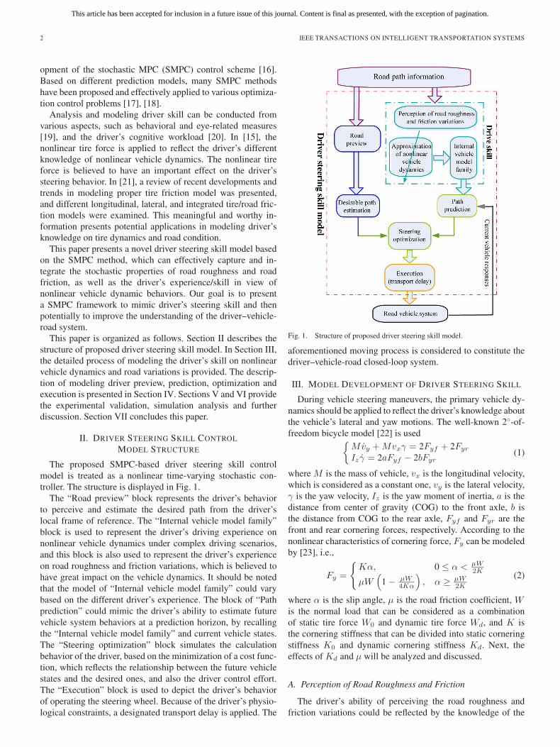
The proposed SMPC-based driver steering skill controlmodel is treated as a nonlinear time-varying stochastic con-troller. The structure is displayed in Fig. 1.

The “Road preview” block represents the driver’s behaviorto perceive and estimate the desired path from the driver’slocal frame of reference. The “Internal vehicle model family”block is used to represent the driver’s driving experience onnonlinear vehicle dynamics under complex driving scenarios,and this block is also used to represent the driver’s experienceon road roughness and friction variations, which is believed tohave great impact on the vehicle dynamics. It should be notedthat the model of “Internal vehicle model family” could varybased on the different driver’s experience. The block of “Pathprediction” could mimic the driver’s ability to estimate futurevehicle system behaviors at a prediction horizon, by recallingthe “Internal vehicle model family” and current vehicle states.The “Steering optimization” block simulates the calculationbehavior of the driver, based on the minimization of a cost func-tion, which reflects the relationship between the future vehiclestates and the desired ones, and also the driver control effort.The “Execution” block is used to depict the driver’s behaviorof operating the steering wheel. Because of the driver’s physio-logical constraints, a designated transport delay is applied. The

Fig. 1. Structure of proposed driver steering skill model.

aforementioned moving process is considered to constitute thedriver–vehicle-road closed-loop system.

III. MODEL DEVELOPMENT OF DRIVER STEERING SKILL

During vehicle steering maneuvers, the primary vehicle dy-namics should be applied to reflect the driver’s knowledge aboutthe vehicle’s lateral and yaw motions. The well-known 2◦-of-freedom bicycle model [22] is used{

Mvy +Mvxγ = 2Fyf + 2Fyr

Iz γ = 2aFyf − 2bFyr(1)

where M is the mass of vehicle, vx is the longitudinal velocity,which is considered as a constant one, vy is the lateral velocity,γ is the yaw velocity, Iz is the yaw moment of inertia, a is thedistance from center of gravity (COG) to the front axle, b isthe distance from COG to the rear axle, Fyf and Fyr are thefront and rear cornering forces, respectively. According to thenonlinear characteristics of cornering force, Fy can be modeledby [23], i.e.,

Fy =

{Kα, 0 ≤ α < μW

2K

μW(

1 − μW4Kα

), α ≥ μW

2K

(2)

where α is the slip angle, μ is the road friction coefficient, Wis the normal load that can be considered as a combinationof static tire force W0 and dynamic tire force Wd, and K isthe cornering stiffness that can be divided into static corneringstiffness K0 and dynamic cornering stiffness Kd. Next, theeffects of Kd and μ will be analyzed and discussed.

A. Perception of Road Roughness and Friction

The driver’s ability of perceiving the road roughness andfriction variations could be reflected by the knowledge of the


QU et al.: SWITCHING-BASED SMPC APPROACH FOR MODELING DRIVER STEERING SKILL 3

dynamic cornering stiffness Kd, which can be divided into

Kd = Kd1 +Kd2 (3)

where

Kd1 =K0

(μ

μref− 1

)(4a)

Kd2 = ηWd (4b)

μref is the reference of road adhesion coefficient, η is thecornering stiffness coefficient. From (4), Kd1 is affected by theroad friction coefficient and Kd2 is affected by Wd. Further-more, the dynamic tire force Wd is affected by road roughness,vehicle speed and vehicle suspension/tire properties. There-fore, the effect of road roughness can be represented by Kd2.Combining (3) and (4a), the cornering stiffness K could bedescribed by

K = K0μ

μref+Kd2. (5)

According to (4b), there is Wd = Kd2/η. Because of W0 =K0/η, the normal load could be formulated as

W = W0 +Wd =K0 +Kd2

η. (6)

Put (5) and (6) into (2), the nonlinear cornering force can berepresented by

Fy=

⎧⎪⎪⎪⎪⎪⎪⎪⎪⎨⎪⎪⎪⎪⎪⎪⎪⎪⎩

(K0

μμref

+Kd2

)α, 0≤α

<μ

K0+Kd2η

2(K0

μμref

+Kd2

)μK0+Kd2

η

×(

1− μ(K0+Kd2)

4η(K0

μμref

+Kd2

)α

), α≥ μ

K0+Kd2η

2(K0

μμref

+Kd2

) .

(7)

Considering that the uncertain parameter μ varies around itsmean μref , by assuming μ = μref in the inequality for α of (7),a further simplified formulation is given as

Fy=

⎧⎪⎨⎪⎩

(K0

μμref

+Kd2

)α, 0≤α< μref

2η

μK0+Kd2

η

(1− μ(K0+Kd2)

4η(K0

μμref

+Kd2

)α

), α≥ μref

2η .

(8)

For a given road, the road roughness and friction coefficientmay not be unchanged, and they could be described by ran-dom variables [24], [25]. In this paper, a uniform distributionand a normal distribution are assumed for the human driver’s

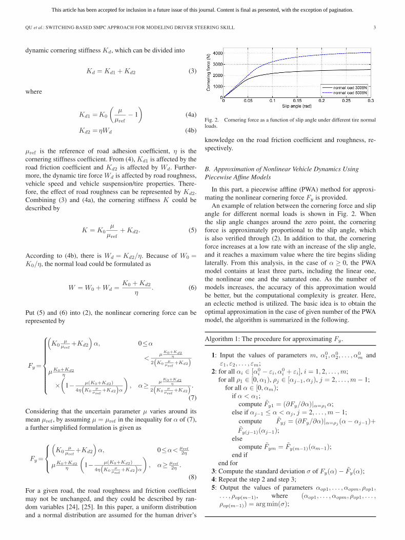
Fig. 2. Cornering force as a function of slip angle under different tire normalloads.

knowledge on the road friction coefficient and roughness, re-spectively.

B. Approximation of Nonlinear Vehicle Dynamics UsingPiecewise Affine Models

In this part, a piecewise affline (PWA) method for approxi-mating the nonlinear cornering force Fy is provided.

An example of relation between the cornering force and slipangle for different normal loads is shown in Fig. 2. Whenthe slip angle changes around the zero point, the corneringforce is approximately proportional to the slip angle, whichis also verified through (2). In addition to that, the corneringforce increases at a low rate with an increase of the slip angle,and it reaches a maximum value where the tire begins slidinglaterally. From this analysis, in the case of α ≥ 0, the PWAmodel contains at least three parts, including the linear one,the nonlinear one and the saturated one. As the number ofmodels increases, the accuracy of this approximation wouldbe better, but the computational complexity is greater. Here,an eclectic method is utilized. The basic idea is to obtain theoptimal approximation in the case of given number of the PWAmodel, the algorithm is summarized in the following.

Algorithm 1: The procedure for approximating Fy .

1: Input the values of parameters m, α01, α

02, . . . , α

0m and

ε1, ε2, . . . , εm;2: for all αi ∈ [α0

i − εi, α0i + εi], i = 1, 2, . . . ,m;

for all ρ1 ∈ [0, α1), ρj ∈ [αj−1, αj), j = 2, . . . ,m− 1;for all α ∈ [0, αm);

if α < α1;compute Fy1 = (∂Fy/∂α)|α=ρ1

α;else if αj−1 ≤ α < αj , j = 2, . . . ,m− 1;

compute Fyj = (∂Fy/∂α)|α=ρj(α− αj−1)+

Fy(j−1)(αj−1);else

compute Fym = Fy(m−1)(αm−1);end if

end for3: Compute the standard deviation σ of Fy(α)− Fy(α);4: Repeat the step 2 and step 3;5: Output the values of parameters αop1, . . . , αopm, ρop1,

. . . , ρop(m−1), where (αop1, . . . , αopm, ρop1, . . . ,ρop(m−1)) = argmin(σ);



TABLE IPIECEWISE RESULTS FOR THE CASES OF m = 4, 5, 6

The PWA model is shown in the equation at the bottom ofthe page.

Notations:m: Given number of PWA model.α00 = 0, α0

1, α02, . . . , α

0m: Initial interval endpoints.

ε1, ε2, . . . , εm: Interval radius.αop0 = 0, αop1, . . . , αopm: Optimal interval endpoints.(∂Fy/∂α)|α=ρopj

,j = 1, 2, . . . ,m− 1: Optimal slopes in the first (m− 1)

intervals.

Remark 1: In algorithm 1, the selected parameters α01, α

02,

. . . , α0m and ε1, ε2, . . . , εm have effects on the optimal approx-

imating method. In order to obtain the better performance ofapproximation, the parameters α0

1, α02, . . . , α

0m could be placed

at the points where the changes of cornering force’s slopes areacute, and the parameter εi, i = 1, 2, . . . ,m, could be selectedin the interval [0,min((α0

i − α0i−1)/2, (α0

i+1 − α0i )/2)].

An example of piecewise approximation results of corneringforce (2) is presented in Table I, it indicates that the 6 PWAmodel has the best approximation result than the others.

From the aforementioned approach, an approximating for-mulation for Fy in (8) can be generalized by

Fy ≈ ξi(Kd2, μ)α+ ζi(Kd2, μ), i = 1, 2, . . . .m (9)

when αf ∈ [αop(i−1), αopi) and αr ∈ [αop(j−1), αopj), i, j =1, 2, . . . ,m, it has

Fyf ≈ ξfiαf + ζfi, Fyr ≈ ξrjαr + ζrj . (10)

Put (10) into (1), there is{Mvy +Mvxγ = 2(ξfiαf + ζfi) + 2(ξrjαr + ζrj)Iz γ = 2a(ξfiαf + ζfi)− 2b(ξrjαr + ζrj)

(11)

it is known that the tire slip angles can be approximated as

αf ≈ vyvx

+aγ

vx− δf , αr ≈ vy

vx− bγ

vx(12)

whereδf is the front steering wheel angle. The state spaceequation can be obtained from (11) and (12) as(vy(t)γ(t)

)=

(2(ξfi+ξrj)

Mvx

2(aξfi−bξrj)Mvx

− vx2(aξfi−bξrj)

Izvx

2(a2ξfi+b2ξrj)Izvx

)(vy(t)γ(t)

)

+

(− 2ξfi

MG

− 2aξfi

IzG

)δ(t) +

(2(ζfi+ζrj)

M2(aζfi−bζrj)

Iz

)(13)

whereδ(t) is the steering wheel angle, and G is the steering gearratio (steering wheel angle/front steering wheel angle). Whenthe yaw displacement ψ is small, the kinematic equations of thevehicle can be simplified as{

x(t) = vx − vy(t)ψ(t)y(t) = vxψ(t) + vy(t)

(14)

where x(t) and y(t) are the longitudinal and lateral displace-ments of the vehicle in ground-fixed axes, respectively.

By combining (13) and (14), when the slip angles αf ∈[αop(i−1), αopi) and αr ∈ [αop(j−1), αopj), the fourth orderstate space equation is given in

X(t) = AijX(t) + Bijδ(t) + Pij (15)

where

X(t) = ( vy(t) γ(t) y(t) ψ(t) )T (16)

Aij =

⎛⎜⎜⎝

2(ξfi+ξrj)Mvx

2(aξfi−bξrj)Mvx

− vx 0 02(aξfi−bξrj)

Izvx

2(a2ξfi+b2ξrj)Izvx

0 01 0 0 vx0 1 0 0

⎞⎟⎟⎠ (17)

Bij =(− 2ξfi

MG − 2aξfi

IzG0 0

)T(18)

Pij =(

2(ζfi+ζrj)M

2(aζfi−bζrj)Iz

0 0)T

. (19)

By defining the output variable

Y (t) = CX(t) = (0 0 1 0) X(t) = y(t) (20)

the vehicle dynamical equations with uncertainties in thecontinuous-time case can be obtained{

X(t) = AijX(t) + Bijδ(t) + Pij

Y (t) = CX(t).(21)

Moreover, the continuous-time uncertain vehicle dynamical(21) can be converted to the discrete-time one using the “zoh”discretization method [26] with sampling period T{

X(k + 1) = AijX(k) +Bijδ(k) + Pij

Y (k) = CX(k).(22)

Fy(α) =

⎧⎪⎪⎪⎨⎪⎪⎪⎩

∂Fy

∂α

∣∣∣α=ρop1

α, αop0 ≤ α < αop1;

∂Fy

∂α

∣∣∣α=ρopj

(α− αop(j−1)

)+ Fy(j−1)

(αop(j−1)

), αop(j−1) ≤ α < αopj , j = 2, . . . ,m− 1;

Fy(m−1)

(αop(m−1)

), αop(m−1) ≤ α < αopm;



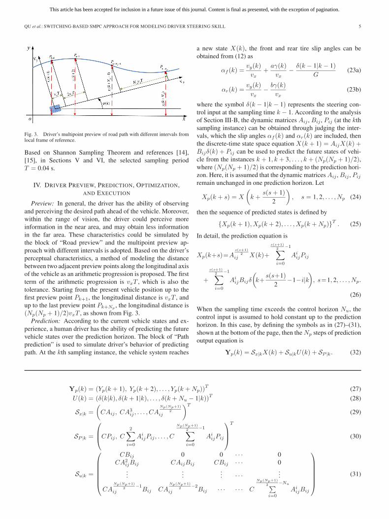
Fig. 3. Driver’s multipoint preview of road path with different intervals fromlocal frame of reference.

Based on Shannon Sampling Theorem and references [14],[15], in Sections V and VI, the selected sampling periodT = 0.04 s.

IV. DRIVER PREVIEW, PREDICTION, OPTIMIZATION,AND EXECUTION

Preview: In general, the driver has the ability of observingand perceiving the desired path ahead of the vehicle. Moreover,within the range of vision, the driver could perceive moreinformation in the near area, and may obtain less informationin the far area. These characteristics could be simulated bythe block of “Road preview” and the multipoint preview ap-proach with different intervals is adopted. Based on the driver’sperceptual characteristics, a method of modeling the distancebetween two adjacent preview points along the longitudinal axisof the vehicle as an arithmetic progression is proposed. The firstterm of the arithmetic progression is vxT , which is also thetolerance. Starting from the present vehicle position up to thefirst preview point Pk+1, the longitudinal distance is vxT , andup to the last preview point Pk+Np

, the longitudinal distance is(Np(Np + 1)/2)vxT , as shown from Fig. 3.

Prediction: According to the current vehicle states and ex-perience, a human driver has the ability of predicting the futurevehicle states over the prediction horizon. The block of “Pathprediction” is used to simulate driver’s behavior of predictingpath. At the kth sampling instance, the vehicle system reaches

a new state X(k), the front and rear tire slip angles can beobtained from (12) as

αf (k) =vy(k)

vx+

aγ(k)

vx− δ(k − 1|k − 1)

G(23a)

αr(k) =vy(k)

vx− bγ(k)

vx(23b)

where the symbol δ(k − 1|k − 1) represents the steering con-trol input at the sampling time k − 1. According to the analysisof Section III-B, the dynamic matrices Aij , Bij , Pij (at the kthsampling instance) can be obtained through judging the inter-vals, which the slip angles αf (k) and αr(k) are included, thenthe discrete-time state space equation X(k + 1) = AijX(k) +Bijδ(k) + Pij can be used to predict the future states of vehi-cle from the instances k + 1, k + 3, . . . , k + (Np(Np + 1)/2),where (Np(Np + 1)/2) is corresponding to the prediction hori-zon. Here, it is assumed that the dynamic matrices Aij , Bij , Pij

remain unchanged in one prediction horizon. Let

Xp(k + s) = X

(k +

s(s+ 1)2

), s = 1, 2, . . . , Np (24)

then the sequence of predicted states is defined by

{Xp(k + 1), Xp(k + 2), . . . , Xp(k +Np)}T . (25)

In detail, the prediction equation is

Xp(k+s)=As(s+1)

2ij X(k)+

s(s+1)2 −1∑i=0

AiijPij

+

s(s+1)2 −1∑i=0

AiijBijδ

(k+

s(s+1)2

−1−i|k), s=1, 2, . . . , Np.

(26)

When the sampling time exceeds the control horizon Nu, thecontrol input is assumed to hold constant up to the predictionhorizon. In this case, by defining the symbols as in (27)–(31),shown at the bottom of the page, then the Np steps of predictionoutput equation is

Yp(k) = Sx|kX(k) + Su|kU(k) + SP |k. (32)

Yp(k) = (Yp(k + 1), Yp(k + 2), . . . , Yp(k +Np))T (27)

U(k) = (δ(k|k), δ(k + 1|k), . . . , δ(k +Nu − 1|k))T (28)

Sx|k =

(CAij , CA3

ij , . . . , CANp(Np+1)

2ij

)T

(29)

SP |k =

⎛⎜⎝CPij , C

2∑i=0

AiijPij , . . . , C

Np(Np+1)

2 −1∑i=0

AiijPij

⎞⎟⎠

T

(30)

Su|k =

⎛⎜⎜⎜⎜⎜⎝

CBij 0 0 · · · 0CA2

ijBij CAijBij CBij · · · 0...

...... · · ·

...

CANp(Np+1)

2 −1ij Bij CA

Np(Np+1)

2 −2ij Bij · · · · · · C

Np(Np+1)

2 −Nu∑i=0

AiijBij

⎞⎟⎟⎟⎟⎟⎠ (31)



Optimization: In order to reflect the vehicle’s tracking per-formance, the driver’s physical workload and mental workload,a cost function consisting of a weighted combination of lateralpath error and ease of driver control is considered as

J(k) =

Np∑i=1

‖Yp(k + i)− yr(k + i)‖2Γy,i

+

Nu−1∑i=0

(‖δ(k + i|k)‖2Γu,i

+ ‖Δδ(k + i|k)‖2ΓΔu,i

)(33)

where

Δδ(k|k) = δ(k|k)− δ(k − 1|k − 1) (34a)

Δδ(k + j|k) = δ(k + j|k)− δ(k + j − 1|k)j = 1, 2, . . . , Nu − 1 (34b)

and yr(k + i) is the lateral displacement of preview pointPk+i in ground-fixed axes. δ(k + i|k), i = 0, 1, . . . , Nu − 1,represents the predicted control input of sampling time k + i atthe present sampling time k.

By defining the symbols as

R(k)= (yr(k+1), yr(k+2), . . . , yr(k+Np))T (35)

ΔU(k)= (Δδ(k|k),Δδ(k+1|k), . . . ,Δδ(k+Nu−1|k))T

(36)

it has

ΔU(k) = LU(k)− Iδ(k − 1|k − 1) (37)

where

I =

⎛⎜⎜⎜⎜⎝

100...0

⎞⎟⎟⎟⎟⎠ , L =

⎛⎜⎜⎜⎜⎝

1 0 0 · · · 0 0−1 1 0 · · · 0 00 −1 1 · · · 0 0...

...... · · ·

......

0 0 0 · · · −1 1

⎞⎟⎟⎟⎟⎠ . (38)

Then the cost function can be described by

J(k) = (Yp(k)−R(k))T Γy (Yp(k)−R(k))

+ UT (k)ΓuU(k) + ΔUT (k)ΓΔuΔU(k) (39)

with the weighting matrices

Γy =diag{Γy,1,Γy,2, . . . ,Γy,Np

}> 0 (40a)

Γu =diag {Γu,0,Γu,1, . . . ,Γu,Nu−1} > 0 (40b)

ΓΔu =diag {ΓΔu,0,ΓΔu,1, . . . ,ΓΔu,Nu−1} > 0. (40c)

By minimizing the conditional expectation of J(k), the optimalcontrol vector sequence U(k) can be determined as

U ∗(k) = argminU(k)∈U

E [J(k)|Y0:k] (41)

where U is the set of all possible control actions, Y0:k =(Y (0), . . . , Y (k))T is the measured output sequence, and

TABLE IIPARAMETER VALUES OF THE HONGQI HQ430

E[J(k)|Y0:k] is the conditional expectation. In general,Kd2(k) is affected by the vertical road roughness profiles, andμ(k) is mostly affected by the horizontal contact characteristicsbetween road surface and tire. In vehicle dynamics, these twoproperties are often assumed to be independent. Then, theoutput sequence Y0:k does not affect the values of the predictedoutputs, it has

E [J(k)|Y0:k] = E [J(k)] (42)

let (∂E[J(k)]/∂U(k)) = 0, it can be deduced that

U ∗(k) ={E

[STu|kΓySu|k

]+ Γu + LTΓΔuL

}−1

× E{STu|kΓy

[R(k)− Sx|kX(k)− SP |k

]+ LTΓΔuIδ(k − 1|k − 1)

}. (43)

After the successful solution of the optimization problem, onlythe first step of the optimal control sequence is applied to thecontrolled vehicle.

Execution: Taking into account the driver’s physiologicalconstraints, a designated transport delay is applied and itstransfer function is designed by D(s) = e−tds, where td is theparameter of transport delay.

V. EXPERIMENTAL VALIDATION AND

PARAMETRIC STUDIES

The aforementioned analytical formulations, together withthe experimental data of HQ430 and commercial vehicle dy-namics software veDYNA, are integrated to validate and ana-lyze the closed-loop driver–vehicle steering responses.

A. Experimental Validation of the Proposed Driver SteeringSkill Model

In this part, the experimental data of Hongqi HQ430(A product of China First Auto Works) are used to validate theproposed driver steering skill model, its parameters are given inTable II.

The experiments are executed for double lane change maneu-ver in the dry and asphalt road. The driver conducted the testsis a 35-year-old male driver, who has more than 12 years’ driv-ing experience. The experimental data: steering wheel angle,longitudinal and lateral accelerations, longitudinal and lat-eral velocities are obtained from CAN Bus, gyroscope



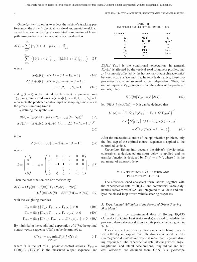
Fig. 4. Experimental measuring instruments.

(INS-NAV420CA-100), and speed sensor (DEWE-VGPS-200C), respectively (the sensors are shown in Fig. 4).

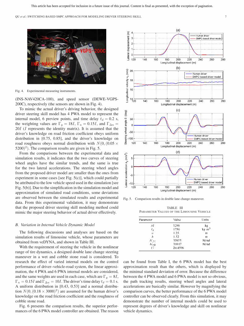
To mimic the actual driver’s driving behavior, the designeddriver steering skill model has 4 PWA model to represent theinternal model, 6 preview points, and time delay td = 0.2 s,the weighting values are Γy = 18I , Γu = 0.15I , and ΓΔu =20I (I represents the identity matrix). It is assumed that thedriver’s knowledge on road friction coefficient obeys uniformdistribution in [0.75, 0.85], and the driver’s knowledge onroad roughness obeys normal distribution with N(0, (0.05 ×5200)2). The comparison results are given in Fig. 5.

From the comparisons between the experimental data andsimulation results, it indicates that the two curves of steeringwheel angles have the similar trends, and the same is truefor the two lateral accelerations. The steering wheel anglesfrom the proposed driver model are smaller than the ones fromexperiment in some cases [see Fig. 5(c)], which could partiallybe attributed to the low vehicle speed used in the simulation [seeFig. 5(b)]. Due to the simplification in the simulation model andapproximation of simulated road conditions, some deviationsare observed between the simulated results and experimentaldata. From this experimental validation, it may demonstratethat the proposed driver steering skill modeling method couldmimic the major steering behavior of actual driver effectively.

B. Variation in Internal Vehicle Dynamic Model

The following discussions and analyses are based on thesimulation results of limousine vehicle, whose parameters areobtained from veDYNA, and shown in Table III.

With the requirement of steering the vehicle in the nonlinearrange of tire dynamics, a designed double lane change steeringmaneuver in a wet and cobble stone road is considered. Toresearch the effect of varied internal models on the controlperformance of driver–vehicle-road system, the linear approxi-mation, the 4 PWA and 6 PWA internal models are considered,and the same weights are used in each case, which are Γy = 8I ,Γu = 0.15I and ΓΔu = 10I . The driver’s time delay td = 0.1 s.A uniform distribution in [0.43, 0.53] and a normal distribu-tion N(0, (0.18 × 3000)2) are assumed for the human driver’sknowledge on the road friction coefficient and the roughness ofcobble stone road.

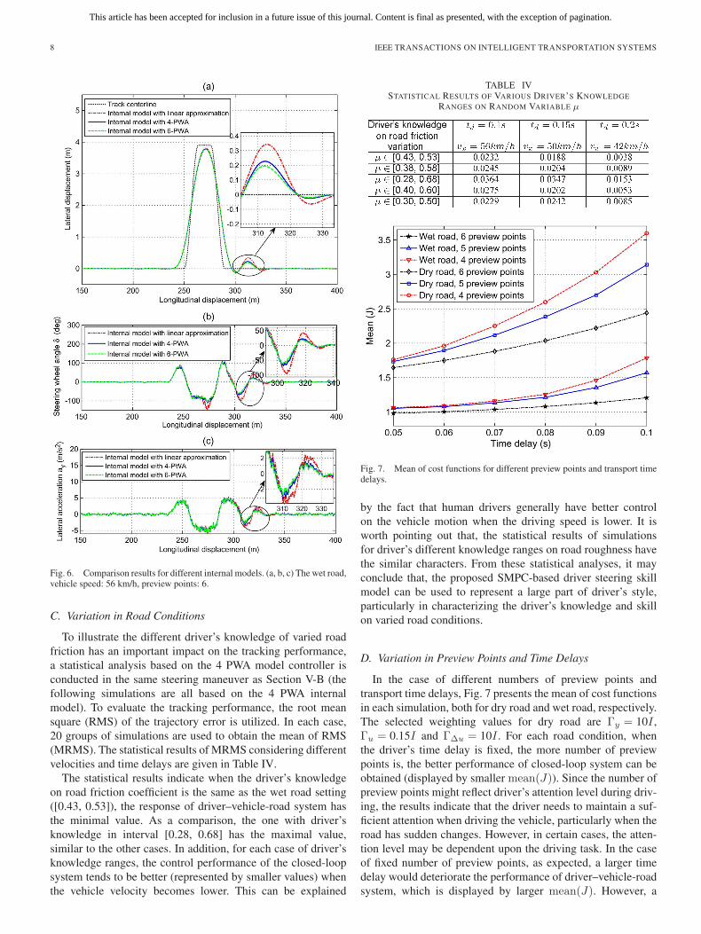
Fig. 6 presents the comparison results, the superior perfor-mances of the 6 PWA model controller are obtained. The reason

Fig. 5. Comparison results in double lane change maneuver.

TABLE IIIPARAMETER VALUES OF THE LIMOUSINE VEHICLE

can be found from Table I, the 6 PWA model has the bestapproximation result than the others, which is displayed bythe minimal standard deviation of error. Because the differencebetween the 4 PWA model and 6 PWA model is not so obvious,the path tracking results, steering wheel angles and lateralaccelerations are basically similar. However by magnifying thecomparison curves, the better performance of the 6 PWA modelcontroller can be observed clearly. From this simulation, it maydemonstrate the number of internal models could be used torepresent degrees of driver’s knowledge and skill on nonlinearvehicle dynamics.



Fig. 6. Comparison results for different internal models. (a, b, c) The wet road,vehicle speed: 56 km/h, preview points: 6.

C. Variation in Road Conditions

To illustrate the different driver’s knowledge of varied roadfriction has an important impact on the tracking performance,a statistical analysis based on the 4 PWA model controller isconducted in the same steering maneuver as Section V-B (thefollowing simulations are all based on the 4 PWA internalmodel). To evaluate the tracking performance, the root meansquare (RMS) of the trajectory error is utilized. In each case,20 groups of simulations are used to obtain the mean of RMS(MRMS). The statistical results of MRMS considering differentvelocities and time delays are given in Table IV.

The statistical results indicate when the driver’s knowledgeon road friction coefficient is the same as the wet road setting([0.43, 0.53]), the response of driver–vehicle-road system hasthe minimal value. As a comparison, the one with driver’sknowledge in interval [0.28, 0.68] has the maximal value,similar to the other cases. In addition, for each case of driver’sknowledge ranges, the control performance of the closed-loopsystem tends to be better (represented by smaller values) whenthe vehicle velocity becomes lower. This can be explained

TABLE IVSTATISTICAL RESULTS OF VARIOUS DRIVER’S KNOWLEDGE

RANGES ON RANDOM VARIABLE μ

Fig. 7. Mean of cost functions for different preview points and transport timedelays.

by the fact that human drivers generally have better controlon the vehicle motion when the driving speed is lower. It isworth pointing out that, the statistical results of simulationsfor driver’s different knowledge ranges on road roughness havethe similar characters. From these statistical analyses, it mayconclude that, the proposed SMPC-based driver steering skillmodel can be used to represent a large part of driver’s style,particularly in characterizing the driver’s knowledge and skillon varied road conditions.

D. Variation in Preview Points and Time Delays

In the case of different numbers of preview points andtransport time delays, Fig. 7 presents the mean of cost functionsin each simulation, both for dry road and wet road, respectively.The selected weighting values for dry road are Γy = 10I ,Γu = 0.15I and ΓΔu = 10I . For each road condition, whenthe driver’s time delay is fixed, the more number of previewpoints is, the better performance of closed-loop system can beobtained (displayed by smaller mean(J)). Since the number ofpreview points might reflect driver’s attention level during driv-ing, the results indicate that the driver needs to maintain a suf-ficient attention when driving the vehicle, particularly when theroad has sudden changes. However, in certain cases, the atten-tion level may be dependent upon the driving task. In the caseof fixed number of preview points, as expected, a larger timedelay would deteriorate the performance of driver–vehicle-roadsystem, which is displayed by larger mean(J). However, a



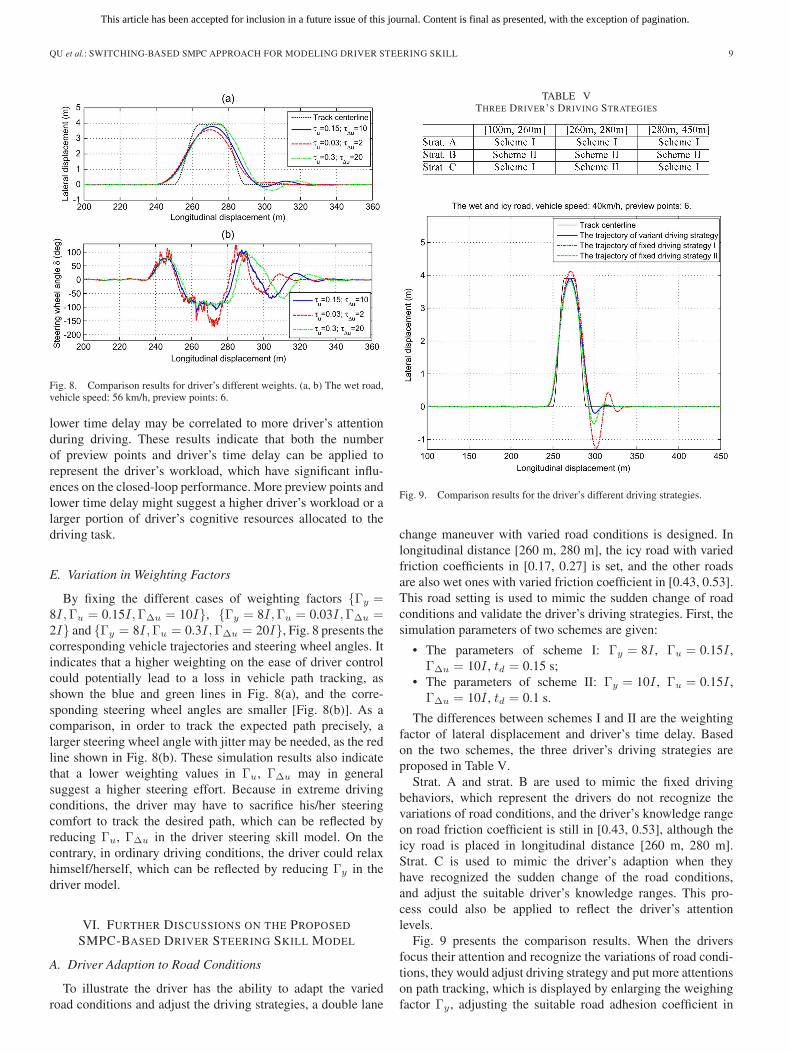
Fig. 8. Comparison results for driver’s different weights. (a, b) The wet road,vehicle speed: 56 km/h, preview points: 6.

lower time delay may be correlated to more driver’s attentionduring driving. These results indicate that both the numberof preview points and driver’s time delay can be applied torepresent the driver’s workload, which have significant influ-ences on the closed-loop performance. More preview points andlower time delay might suggest a higher driver’s workload or alarger portion of driver’s cognitive resources allocated to thedriving task.

E. Variation in Weighting Factors

By fixing the different cases of weighting factors {Γy =8I,Γu = 0.15I,ΓΔu = 10I}, {Γy = 8I,Γu = 0.03I,ΓΔu =2I} and {Γy = 8I,Γu = 0.3I,ΓΔu = 20I}, Fig. 8 presents thecorresponding vehicle trajectories and steering wheel angles. Itindicates that a higher weighting on the ease of driver controlcould potentially lead to a loss in vehicle path tracking, asshown the blue and green lines in Fig. 8(a), and the corre-sponding steering wheel angles are smaller [Fig. 8(b)]. As acomparison, in order to track the expected path precisely, alarger steering wheel angle with jitter may be needed, as the redline shown in Fig. 8(b). These simulation results also indicatethat a lower weighting values in Γu, ΓΔu may in generalsuggest a higher steering effort. Because in extreme drivingconditions, the driver may have to sacrifice his/her steeringcomfort to track the desired path, which can be reflected byreducing Γu, ΓΔu in the driver steering skill model. On thecontrary, in ordinary driving conditions, the driver could relaxhimself/herself, which can be reflected by reducing Γy in thedriver model.

VI. FURTHER DISCUSSIONS ON THE PROPOSED

SMPC-BASED DRIVER STEERING SKILL MODEL

A. Driver Adaption to Road Conditions

To illustrate the driver has the ability to adapt the variedroad conditions and adjust the driving strategies, a double lane

TABLE VTHREE DRIVER’S DRIVING STRATEGIES

Fig. 9. Comparison results for the driver’s different driving strategies.

change maneuver with varied road conditions is designed. Inlongitudinal distance [260 m, 280 m], the icy road with variedfriction coefficients in [0.17, 0.27] is set, and the other roadsare also wet ones with varied friction coefficient in [0.43, 0.53].This road setting is used to mimic the sudden change of roadconditions and validate the driver’s driving strategies. First, thesimulation parameters of two schemes are given:

• The parameters of scheme I: Γy = 8I , Γu = 0.15I ,ΓΔu = 10I , td = 0.15 s;

• The parameters of scheme II: Γy = 10I , Γu = 0.15I ,ΓΔu = 10I , td = 0.1 s.

The differences between schemes I and II are the weightingfactor of lateral displacement and driver’s time delay. Basedon the two schemes, the three driver’s driving strategies areproposed in Table V.

Strat. A and strat. B are used to mimic the fixed drivingbehaviors, which represent the drivers do not recognize thevariations of road conditions, and the driver’s knowledge rangeon road friction coefficient is still in [0.43, 0.53], although theicy road is placed in longitudinal distance [260 m, 280 m].Strat. C is used to mimic the driver’s adaption when theyhave recognized the sudden change of the road conditions,and adjust the suitable driver’s knowledge ranges. This pro-cess could also be applied to reflect the driver’s attentionlevels.

Fig. 9 presents the comparison results. When the driversfocus their attention and recognize the variations of road condi-tions, they would adjust driving strategy and put more attentionson path tracking, which is displayed by enlarging the weighingfactor Γy , adjusting the suitable road adhesion coefficient in



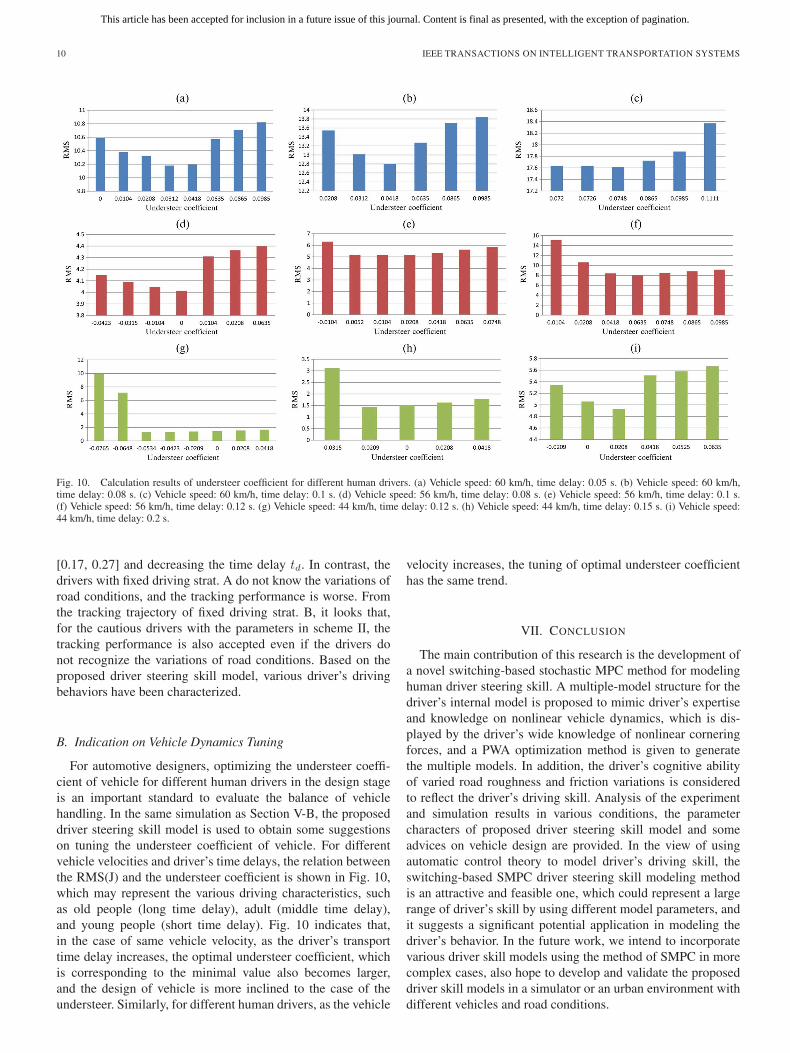
Fig. 10. Calculation results of understeer coefficient for different human drivers. (a) Vehicle speed: 60 km/h, time delay: 0.05 s. (b) Vehicle speed: 60 km/h,time delay: 0.08 s. (c) Vehicle speed: 60 km/h, time delay: 0.1 s. (d) Vehicle speed: 56 km/h, time delay: 0.08 s. (e) Vehicle speed: 56 km/h, time delay: 0.1 s.(f) Vehicle speed: 56 km/h, time delay: 0.12 s. (g) Vehicle speed: 44 km/h, time delay: 0.12 s. (h) Vehicle speed: 44 km/h, time delay: 0.15 s. (i) Vehicle speed:44 km/h, time delay: 0.2 s.

[0.17, 0.27] and decreasing the time delay td. In contrast, thedrivers with fixed driving strat. A do not know the variations ofroad conditions, and the tracking performance is worse. Fromthe tracking trajectory of fixed driving strat. B, it looks that,for the cautious drivers with the parameters in scheme II, thetracking performance is also accepted even if the drivers donot recognize the variations of road conditions. Based on theproposed driver steering skill model, various driver’s drivingbehaviors have been characterized.

B. Indication on Vehicle Dynamics Tuning

For automotive designers, optimizing the understeer coeffi-cient of vehicle for different human drivers in the design stageis an important standard to evaluate the balance of vehiclehandling. In the same simulation as Section V-B, the proposeddriver steering skill model is used to obtain some suggestionson tuning the understeer coefficient of vehicle. For differentvehicle velocities and driver’s time delays, the relation betweenthe RMS(J) and the understeer coefficient is shown in Fig. 10,which may represent the various driving characteristics, suchas old people (long time delay), adult (middle time delay),and young people (short time delay). Fig. 10 indicates that,in the case of same vehicle velocity, as the driver’s transporttime delay increases, the optimal understeer coefficient, whichis corresponding to the minimal value also becomes larger,and the design of vehicle is more inclined to the case of theundersteer. Similarly, for different human drivers, as the vehicle

velocity increases, the tuning of optimal understeer coefficienthas the same trend.

VII. CONCLUSION

The main contribution of this research is the development ofa novel switching-based stochastic MPC method for modelinghuman driver steering skill. A multiple-model structure for thedriver’s internal model is proposed to mimic driver’s expertiseand knowledge on nonlinear vehicle dynamics, which is dis-played by the driver’s wide knowledge of nonlinear corneringforces, and a PWA optimization method is given to generatethe multiple models. In addition, the driver’s cognitive abilityof varied road roughness and friction variations is consideredto reflect the driver’s driving skill. Analysis of the experimentand simulation results in various conditions, the parametercharacters of proposed driver steering skill model and someadvices on vehicle design are provided. In the view of usingautomatic control theory to model driver’s driving skill, theswitching-based SMPC driver steering skill modeling methodis an attractive and feasible one, which could represent a largerange of driver’s skill by using different model parameters, andit suggests a significant potential application in modeling thedriver’s behavior. In the future work, we intend to incorporatevarious driver skill models using the method of SMPC in morecomplex cases, also hope to develop and validate the proposeddriver skill models in a simulator or an urban environment withdifferent vehicles and road conditions.



REFERENCES

[1] L. Li, D. Wen, N. N. Zheng, and L. C. Shen, “Cognitive cars: A newfrontier for ADAS research,” IEEE Trans. Intell. Transp. Syst., vol. 13,no. 1, pp. 395–407, Mar. 2012.

[2] J. Q. Wang, L. Zhang, D. Z. Zhang, and K. Q. Li, “An adaptive longi-tudinal driving assistance system based on driver characteristics,” IEEETrans. Intell. Transp. Syst., vol. 14, no. 1, pp. 1–12, Mar. 2013.

[3] F. Y. Wang, “Parallel control and management for intelligent transporta-tion systems: Concepts, architectures, applications,” IEEE Trans. Intell.Transp. Syst., vol. 11, no. 3, pp. 630–638, Sep. 2010.

[4] J. P. Zhang et al., “Data-driven intelligent transportation systems: A sur-vey,” IEEE Trans. Intell. Transp. Syst., vol. 12, no. 4, pp. 1624–1639,Dec. 2011.

[5] B. Z. Gao, H. Chen, K. Sanada, Y. F. Hu, and P. W. Daly, “De-sign of clutch-slip controller for automatic transmission using backstep-ping,” IEEE/ASME Trans. Mechatronics, vol. 16, no. 3, pp. 498–508,Jun. 2011.

[6] C. C. Macadam, “Understanding and modeling the human driver,” Veh.Syst. Dyn., vol. 40, no. 1–3, pp. 101–134, Sep. 2003.

[7] M. Plöhl and J. Edelmann, “Driver models in automobile dynamics appli-cation,” Veh. Syst. Dyn., vol. 45, no. 7–8, pp. 699–741, Jul./Aug. 2007.

[8] B. Thierry, B. A. Beatrice, M. Pierre, and B. Aurelie, “A theoretical andmethodological framework for studying and modeling drivers’ mentalrepresentations,” Safety Sci., vol. 47, no. 9, pp. 1205–1221, Nov. 2009.

[9] H. Chen and F. Allgower, “A quasi-infinite horizon nonlinear model pre-dictive control scheme with guaranteed stability,” Automatica, vol. 34,no. 10, pp. 1205–1217, Oct. 1998.

[10] D. Hrovat, S. Di Cairano, H. E. Tseng, and I. V. Kolmanovsky, “The de-velopment of model predictive control in automotive industry: A survey,”in Proc. IEEE Int. Conf. Control Appl., Oct. 3–5, 2012, pp. 295–302.

[11] C. C. MacAdam, “An optimal preview control for linear systems,” Trans.ASME, J. Dyn. Syst. Meas. Control, vol. 102, no. 3, pp. 188–190,Sep. 1980.

[12] C. C. MacAdam, “Application of an optimal preview control for simula-tion of closed-loop automobile driving,” IEEE Trans. Syst., Man Cybern.,vol. 11, no. 6, pp. 393–399, Jun. 1981.

[13] A. Y. Ungoren and H. Peng, “An adaptive lateral preview driver model,”Veh. Syst. Dyn., vol. 43, no. 4, pp. 245–259, Apr. 2005.

[14] D. J. Cole, A. J. Pick, and A. M. C. Odhams, “Predictive and linearquadratic methods for potential application to modeling driver steeringcontrol,” Veh. Syst. Dyn., vol. 44, no. 3, pp. 259–284, Mar. 2006.

[15] S. D. Keen and D. J. Cole, “Application of time-variant predictivecontrol to modeling driver steering skill,” Veh. Syst. Dyn., vol. 49, no. 4,pp. 527–559, Apr. 2011.

[16] D. Bernardini and A. Bemporad, “Stabilizing model predictive controlof stochastic constrained linear systems,” IEEE Trans. Autom. Control,vol. 57, no. 6, pp. 1468–1480, Jun. 2012.

[17] G. Ripaccioli, D. Bernardini, S. Di Cairano, A. Bemporad, andI. V. Kolmanovsky, “A stochastic model predictive control approach forseries hybrid electric vehicle power management,” in Proc. Amer. ControlConf., Baltimore, MD, USA, Jun./Jul. 2010, pp. 5844–5849.

[18] Y. D. Ma, S. Vichik, and F. Borrelli, “Fast stochastic MPC with optimalrisk allocation applied to building control systems,” in Proc. 51st IEEEConf. Decision Control, Maui, HI, USA, Dec. 2012, pp. 7559–7564.

[19] L. Li et al., “Behavioral and eye-movement measures to track improve-ments in driving skills of vulnerable road users: First-time motorcycleriders,” Trans. Res. F, Traffic Psychol. Behav., vol. 14, no. 1, pp. 26–35,Jan. 2011.

[20] C. J. D. Patten, A. Kircher, J. Ostlund, and O. Svenson, “Driver experienceand cognitive workload in different traffic environments,” Accid. Anal.Prev., vol. 38, no. 5, pp. 887–894, Sep. 2006.

[21] L. Li, F. Y. Wang, and Q. Zhou, “Intergrated longitudinal and lateraltire/road friction modeling and monitoring for vehicle motion control,”IEEE Trans. Intell. Transp. Syst., vol. 7, no. 1, pp. 1–19, Mar. 2006.

[22] S. B. Zheng, H. J. Tang, Z. Z. Han, and Y. Zhang, “Controller designfor vehicle stability enhancement,” Control Eng. Pract., vol. 14, no. 12,pp. 1413–1421, Dec. 2006.

[23] J. Y. Wong, Theory of Ground Vehicles3rd ed. Hoboken, NJ, USA:Wiley, 2001.

[24] I. Juga, P. Nurmi, and M. Hippi, “Statistical modeling of wintertime roadsurface friction,” Meteorol. Appl., vol. 20, no. 3, pp. 318–329, Sep. 2012.

[25] E. L. Izeppi, G. W. Flintsch, and K. K. McGhee, “Field Performance OfHigh Friction Surfaces,” Virginia Tech. Transp. Inst., Blacksburg, VA,USA, FHWA/VTRC 10-CR6, 2010.

[26] C. T. Chen, Linear System Theory and Design. London, U.K.: OxfordUniv. Press, 1995.

Ting Qu received the B.S. and M.S. degrees fromNortheast Normal University, Changchun, China, in2006 and 2008, respectively. She is currently work-ing toward the Ph.D. degree in control science andengineering at Jilin University of China, Changchun.

Her research interests include model predictivecontrol and driver modeling.

Hong Chen received the B.S. and M.S. de-grees in process control from Zhejiang University,Hangzhou, China, in 1983 and 1986, respectively, andthe Ph.D. degree from University of Stuttgart,Stuttgart, Germany, in 1997.

In 1986 she joined Jilin University of Technology,Changchun, China. From 1993 to 1997 she wasa Wissenschaftlicher Mitarbeiter with Institut fuerSystemdynamik und Regelungstechnik, Universityof Stuttgart. Since 1999 she has been a Professorwith Jilin University, where she is presently a Tang

Aoqing Professor. Her research interests include model predictive control,optimal and robust control, and applications in process engineering and mecha-tronic systems.

Dongpu Cao received the Ph.D. degree from Con-cordia University, Montreal, QC, Canada, in 2008.

He is a Lecturer with the Centre for AutomotiveEngineering, Cranfield University, Bedford, U.K.His research focuses mainly on electric/hybrid vehi-cles, vehicle dynamics and control, driver modeling,and intelligent vehicles, where he has contributed 4coedited journal special editions, 1 patent, and about70 publications.

Dr. Cao received the ASME AVTT2010 Best Pa-per Award and the 2012 SAE Arch T. Colwell Merit

Award. He is an Editor for IEEE TRANSACTIONS ON VEHICULAR TECH-NOLOGY, an Associate Editor for IEEE TRANSACTIONS ON INDUSTRIAL

ELECTRONICS, and an Editorial Board member for another 5 journals. He hasbeen a Guest Editor for Vehicle System Dynamics (2008–2010), IEEE/ASMETransactions on Mechatronics (2014–2015), and IEEE TRANSACTIONS ON

INDUSTRIAL INFORMATICS (2014–2015).

Hongyan Guo received the B.S. and M.S. degreesfrom the University of Science and TechnologyLiaoning, Anshan, China, in 2004 and 2007, respec-tively, and the Ph.D. degree from Jilin University,Changchun, China, in 2010.

She is a Lecturer with the Department of ControlScience and Engineering, Jilin University. Her re-search interests include vehicle states estimation andstability controls.

Bingzhao Gao received the B.S. and M.S. degreesfrom Jilin University of Technology, Changchun,China, in 1998 and Jilin University, Changchun, in2002, respectively, and the Ph.D. degrees in mechan-ical engineering from Yokohama National Univer-sity, Yokohama, Japan, and control engineering fromJilin University, China, in 2009.

He is a professor with Jilin University. His re-search interests include vehicle powertrain control,and vehicle stability control.

Documents

Switching-Based Stochastic Model Predictive Control Approach for Modeling Driver Steering Skill