Sydney Water:

Pricing for Sustainability

R. Quentin Grafton and Tom Kompas

Australian National University

Economics and Environment Network Working Paper EEN0609

October 2006

DRAFT

Sydney Water: Pricing for Sustainability1

R. Quentin Grafton* Crawford School of Economics and Government

The Australian National University

Tom Kompas Crawford School of Economics and Government

The Australian National University and

Australian Bureau of Agricultural and Resource Economics

*contact author: J.G Crawford Building (13), Ellery Crescent, Canberra ACT 0200, Australia. quentin.grafton@anu.edu.au, fax +61-2-6125-5570, tel: +61-2-6125-6558.

October 2006

DRAFT

1

Abstract

We examine how scarcity pricing can be used to assist with urban water demand

management in Sydney in low rainfall periods using an estimated aggregate daily

water demand function. Modelling shows that current water supplies and water prices

are inadequate to prevent Sydney reaching critically low water storage levels should

there be a low rainfall period similar to what occurred in 2001-2005. Simulations

indicate that, in low rainfall periods, the water price needed to balance supply and

demand exceeds the marginal cost of supplying desalinised water. The policy

implication is that even with expected increases in supply (groundwater withdrawals,

recycling), Sydney water prices must be substantially raised over their current levels,

preferably at pre-defined water storage trigger levels, in response to low rainfall

periods.

Keywords: water, pricing, sustainability

JEL codes: Q21, Q25

2

Australian cities are currently facing severe, and in most cases chronic, shortages of

water, relative to the demand at prevailing prices.

John Quiggin (2006, p. 14)

1. Introduction

Many of Australia’s urban water consumers are obliged to follow water restrictions in

terms of when they can use water, and for what purposes (Quiggin 2006). These

quantitative restrictions are in response to an imbalance between expected supply and

demand that is caused by various factors, including a lack of investment in water

infrastructure supply in the past 20 years (Dwyer 2006), increasing urban population,

regulatory restrictions on rural-urban water trading (Productivity Commission 2006),

and urban water pricing that fails to account for large temporal variations in supply.

Using daily water demand data and dam levels in the Sydney catchment, we estimate

an aggregate water demand model and undertake scenario analysis of the effects of

different urban water pricing and additional sources of supply on total water storage.

The results indicate that, even with expected supply increases, the scheduled water

prices are not sufficiently high enough to balance supply and demand should there be

another low rainfall period similar to that which occurred over 2001-2004. An

alternative water pricing model for Sydney based on the amount of water in the

catchment, with pre-set trigger and volumetric prices and possibly a fixed fee

connection charge, is recommended as a short to medium term response to balance

supply and demand.

In Section 2 we review the supply, demand and pricing issues in Sydney water.

Section 3 provides estimates of the aggregate daily water demand we use to simulate

the increase in water prices that would have been required to keep storage levels

above given levels over the period 2001-2005. Section 4 explores the effects of

different water prices and supply scenarios over the next four years beginning at

current water storage levels (40%) and assuming the rainfall and evaporation pattern

that occurred over the 2001-2005 period were repeated. Section 5 provides policy

3

implications in terms of supply and demand management, especially water pricing, in

low rainfall periods. Section 6 concludes.

2. Sydney Water: Background

The water used to supply urban consumers in the greater Sydney area is owned and

operated by the Sydney Catchment Authority (SCA) that is a New South Wales

(NSW) government agency. SCA provides the infrastructure and storage to supply

bulk customers who then filter and distribute the water to retail customers. The retail

water distributor is Sydney Water — a NSW state-owned corporation that supplies

households with drinking water, wastewater and stormwater services and recycled

water.

The NSW Independent Pricing and Regulatory Tribunal (IPART) set the maximum

retail price for water in Sydney. Its stated preference is to set water prices with

reference to the long-run marginal cost of supply (LRMC) which it estimates to be

between $1.20-1.50 per kilolitre (KL) in 2004/2005 (IPART 2005, p. 18). In its latest

determination that sets prices until 30 June 2009 IPART also stated that water pricing

should account for the “…imbalance between the demand for water and the available

supply…” (IPART 2005, p. 105). To this end, the Tribunal recently established a two-

tier increasing block pricing system where the higher Tier 2 price is imposed when

households exceed a 100 KL per quarter. These scheduled water price charges are

given in Table 1. The 2005/2006 Tier 1 price of $1.20/KL represents a 70% increase

from its level in 1995/96 of $0.70/KL.

The Sydney water supply is determined by the quantity of water in the dams owned

by the SCA that changes on a daily basis. The last time the overall dam level was at

100% capacity was in 1998. There have been substantial falls in water levels

(measured as a percentage of total capacity) in the second half of 2002 (dropping from

around 80% to about 60% of capacity) and the first half 2004 (dropping from around

60% to less than 50% of capacity). There are 11 dams that supply water for Sydney,

and the largest is the Warragamba Dam. It is by far the biggest in terms of its overall

capacity and has suffered the greatest declines of water in storage in the past five

4

years. As of October 2006, the total water available in the dams is a little over 1,000

billion litres (GL), or about 40% of the total water storage capacity of some 2,500 GL.

Water supply and demand are negatively correlated because low rainfall and high

temperatures that reduce supply also coincide with greater water demand. This makes

balancing supply with demand a difficult task in a variable climate subject to

extended periods of low rainfall. The supply challenge is aggravated by the fact that

an additional dam in the catchment would take upwards of a decade to build and fill

under normal rainfall conditions, and up to 30 years in low rainfall periods at a cost in

excess of $2 billion (New South Wales Government 2004).

Median yields or net inflows into the Sydney catchment are a little less than 600

GL/year, but can be much less in low rainfall period (NSW Government 2004). For

instance, net physical inflows in 2004 were 314 GL while the total consumption was

539 GL. An increasing population, expected to be more about 20% higher in a little

over 20 years, and a predicted decline in net inflows due to climate change are both

expected to make the balancing of supply and demand even more difficult in the

future (Young et al. 2006).

To help address supply concerns, the NSW government initiated water restrictions in

October 2003 and then implemented Level III restrictions in June 2005 — still in

force as of October 2006. Current restrictions include limits on the watering of

gardens to Wednesday and Sunday before 10am and after 4pm, no hosing of hard

surfaces or vehicles, and permits to fill a pool larger than 10 KL (Sydney Water

2006). In addition, there have been subsidies to households to retrofit water efficient

products and install rainwater tanks as well as building codes on new dwellings

designed to reduce water consumption by 40% compared to the current household

average for Sydney (NSW Government 2004).

On the supply side, the SCA has undertaken major capital works to access deep water

at the Warragamba and Nepean dams that allows for the use of previously

inaccessible water of about 40 GL. Groundwater supplies have also been identified

that might be sustainably withdrawn at about 5-10 GL per year, and possibly more for

temporary periods during droughts (SCA 2006). In addition, recycling investments are

5

under way that, by 2015, are expected to deliver up to 70GL/year in additional supply

(NSW Government 2004, 2006). A range of other possible supply measures also

exist, although not currently supported by the NSW government, that include major

diversions from the Shoalhaven River that could provide up to 80 GL/year and a

desalination plant that has been planned to provide between 30-70 GL/year, but with

additional investment could provide up to 180 GL/year.

3. Estimating and Forecasting Sydney Water Demand

To forecast the effect of IPART pricing and to simulate alternative pricing

arrangements on water storage in Sydney we need to estimate aggregate water

demand. Using data from the period 20/10/2001-30/09/2005 we estimate aggregate

daily water demand (DEM) from the Sydney catchment as a function of residential

water prices (LNP), daily temperature (LNT) and daily rainfall (RAIN) data from the

Sydney Observatory, and a dummy variable (DUM1) for water restrictions that began

in October 2003.The starting point of the data coincides with the beginning of the

most recent low rainfall period, and the end point is immediately before the

implementation of two-tier block pricing that began 1 October 2005.

The estimated coefficients and diagnostics of the demand model are provided in Table

2. All variables are in natural logs with the exception of rainfall because of zero

values. The estimated model includes a first order autoregressive process, and we

reject the null hypothesis that water demand and temperature have a unit root. As the

model is in natural logs, the estimated coefficient on the price variable is a point

estimate of the aggregate elasticity of demand. All estimated coefficients are

statistically significant from zero at the 1% level of significance.

The results show, as expected, that an increase in daily rainfall or a decrease in daily

temperature reduce water demand. The estimated coefficient for the dummy variable

indicates that water restrictions appear to have reduced water by about 10%. The

estimated price elasticity of demand of –0.35 equals the median estimate of price

elasticities from a meta-sample of 296 price elasticities from around the world

collected and analysed by Dalhuisen et al. (2003), but is less elastic than the

household demand for water in Brisbane of some -0.507 (Hoffman et al. 2006).

6

To test the forecast reliability of the estimated model we generated an out-of-sample

forecast of the actual daily water storage in the Sydney catchment over the period

1/10/2005-30/06/2006 using the following identity:

Δ forecast water storage = net water inflows – forecast water demand (1)

For the forecast, net daily water inflows are calculated as the difference between the

actual daily water demand and the change in actual daily water storage. A comparison

of the forecast and actual water storage in the Sydney catchment is provided in Figure

1. It shows that the estimated demand provides a good forecast of actual water storage

and this is supported by a very low Mean Absolute Percentage Error of about 1%, and

a Theil inequality coefficient of 0.006 (Makridakis et al. 1998).

The estimated demand can also be used to examine what would have been the

percentage increase in the water price over the actual price required to keep the water

storage in the Sydney catchment above key thresholds (60, 55, 50, 45 and 40% of full

capacity) in the sample period 2001-2005. These price increases are provided in Table

3, using the estimated price elasticity equal to –0.352, and one and two standard errors

above and below this point estimate. The results indicate that the more inelastic the

demand and the higher the minimum water storage level, the greater the increase in

price that is required to achieve a given storage level. Table 3 shows that, given a

water price elasticity of –0.352, the water price would needed to have been almost

80% higher over the period 2001-2005 to have kept the water storage levels above

55% of capacity. This would have avoided imposition of water restrictions that were

triggered at the storage level. Using the -0.352 elasticity, Figure 2 illustrates the actual

water storage over the 2001-2005 period and compares it to what it would have been

with an almost 50% increase in price that would have kept storage levels above half

of full capacity

Table 4 is constructed in the same way as Table 3, but with a hypothetical 50%

increase in the net physical inflows that actually occurred over the period 2001-2005.

It shows that in ‘normal’ rainfall years the existing pricing arrangements would have

been sufficient to keep storage levels between 55-60%. Thus, the problem of

7

balancing supply and demand is primarily an issue during extended periods of low

rainfall.

4. Simulations of Alternative Water Scenarios

The key issue facing water consumers in Sydney is to ensure that supply matches

demand in low rainfall periods. If we use the actual daily net physical inflows over the

period 2001-2005, we can simulate water storage levels over the next four years if we

assume the same net physical inflows are repeated. This allows us to evaluate the

effects of different supply and pricing arrangements on expected water storage levels

in a low rainfall period.

We examine four scenarios assuming that the net physical inflows over the period

2001-2005 are repeated from October 2006 until October 2010. Should the net

physical inflows be greater than what occurred over 2001-2005 then water storage

levels would be correspondingly higher and price increases needed to balance supply

and demand would be lower.

In all four cases we use the scheduled IPART prices that are set until June 2009 given

in Table 1, and assume the consumer price index increases by 3%/year. All scenarios

begin with the actual water storage level as of October 2006 of 40%.

Scenario One

In this scenario, we forecast the actual water storage levels with the IPART scheduled

prices plus we allow for an increase in water supplies from ground water of 15

GL/year (SCA 2006) and from recycling initiatives of 25 GL/year (NSW Government

2004). The hypothetical storage with and without the extra water supplies is presented

in Figure 3. The results indicate that in the absence of extra water supplies beyond the

projected 39 GL/year, or other demand control measures beyond existing water

restrictions, water storage levels could be as low as 25% by 2010 if the rainfall and

temperature pattern in the past four years were repeated. At this point, should low

rainfall conditions continue, it is possible for Sydney to exhaust water supplies in its

dams in about 12 months. This finding is disturbing because it suggests that the

8

current plans to balance water supply and demand in Sydney are insufficient in low

rainfall periods, and could also place Sydney at a point of critical water supply

availability within the next four years.

Scenario Two

In this scenario we simulate an increase in the scheduled IPART price of 48.48%

along with a 39GL/year increase in supply. The 48.48% price increase is the price rise

required over the period 2001-2005 to keep water storage levels above 50%. The

results, shown in Figure 4, indicate that although the almost 50% price increase keeps

water storage levels above 30% it is insufficient to match supply with demand. Under

this scenario, water storage levels are expected to fall from 40% to about 30% over

the four-year projection.

Scenario Three

The NSW government has announced a number of water supply initiatives over the

next 5-10 years that involve several different recycling projects. These projects

combined are expected to increase water supplies by about 70GL/year by 2015 (NSW

Government 2006). In the simulation, we assume these supplies are available

immediately along with groundwater supplies of 15GL/year, and we also increase the

IPART schedules price by almost 50%. Figure 5 shows that even with these

substantial increases in supply and large price increases water storage levels would

continue to fall in low rainfall periods — declining from 40% to about 33%. It

suggests that the current supply planning, even with a large price increase and current

water restrictions, is not sufficient to balance supply and demand in periods of low

rainfall.

Scenario Four

Figure 6 presents simulations that are identical to Scenario 5, but with an additional

supply of 50GL/year from a desalination plant. Although a desalination plant is not

currently planned for Sydney the simulations show that such a plant coupled with a

9

50% price increase, recycling initiatives and use of groundwater supples is sufficient

to match supply with demand in low rainfall periods.

5. Policy Implications

The simulations indicate that in low rainfall periods Sydney’s current planned water

supply increases and scheduled water prices are insufficient to prevent water storage

levels reaching critical thresholds. The modelling shows that it is only through

substantial increases in the water supply and also the price of water will supply match

demand in low rainfall periods. This provides a number of policy implications

regarding supply and demand management of Sydney water.

Water Pricing

The variability in rainfall within Sydney Catchment and the time lag required to build

and fill a new dam suggests that demand management and non-traditional sources of

water are required. In particular, the water price paid by consumers should reflect its

scarcity value that depends on the level of water storage. By contrast, under current

pricing arrangements the scheduled prices are set independently of water storage

levels, and demand is primarily managed through quantitative controls imposed via

water restrictions. Although water restrictions reduced demand by about 10% since

2003 they impose considerable burdens on consumers have failed to balance supply

and demand. Quantity restrictions also prevent water from being allocated on the

basis of marginal willingness to pay (Griffin 2006). In other words, there are likely

high value uses of water for some individuals that are no longer possible with water

restrictions.

An alternative to water restrictions is to use the water price to provide signals to

consumers to adjust their demand depending on the water storage in the Sydney

catchment. In theory, a first-best pricing scheme for a monopoly provider given fixed

capacity and declining average cost is to set the price (P) equal to the marginal cost

(MC) of supply. As this will result in a net loss to the supplier, the difference can

made-up by a lump sum payment allocated among all consumers (Tresch 2002).

10

Renzetti (1992) has modified the first-best pricing rule for urban water delivery. He

argues that the price should equal its long-run marginal cost (LRMC) in peak demand

periods, and equal the short-run marginal cost (SRMC) in off-peak demand periods. In

the case where peak demand exceeds existing capacity, the price in peak periods

should be even higher to ensure demand equals supply.

We propose a modification to the peak-load pricing proposed by Renzetti (1992)

where water prices are adjusted every quarter depending on water in storage in the

Sydney catchment. Under our pricing arrangement the volumetric water charge

should be raised sufficiently to prevent water storage levels going below critical

threshold levels. When water storage is at full capacity, the volumetric price charged

to consumers would equal the short-run marginal cost of supplying water from the

SCA dams. As water storage declines, perhaps at 5% levels (95, 90, 85, 80… of full

capacity), the price of water would increase to reflect increased water scarcity, and

may have to rise very substantially (upwards of 50% of scheduled IPART prices) in

extended low rainfall periods. This proposed pricing structure is given below:

P = SRMC at 95-100% full storage capacity,

P = P* when water storage < 95% such that aggregate demand ensures water storage

does not exceeds critical minimum threshold (2)

Our proposed pricing arrangement is similar to that discussed by Sibley (2006a),

Crase and Dollery (2006) and also Grafton and Kompas (2006) in terms of urban

water pricing for Australia. A common characteristic in all of these proposals is that

the volumetric price of water should be used to ensure demand equals supply, and to

provide appropriate signals and incentives to consumers to reduce demand at periods

of low supply.

Sibley (2006a) has argued that a fixed connection charge might also need to be

applied to ensure a residual revenue component when water is priced at SRMC. Such

a fixed connection charge need not be the identical across households and could even

be related to property values (Sibley 2006b). A fixed connection charge, however,

may not be necessary if there are sufficient low rainfall events as the revenues

11

generated when scarcity prices are applied could more than offset potential losses

when storage is at full capacity.

A potential drawback to scarcity pricing is the high price that consumers, especially

low-income households, will need to pay in low rainfall periods. It is probably for this

reason, based on a survey commissioned by IPART undertaken in 2005, that scarcity

pricing was opposed by about 50% of respondents although supported by about 40%

of those surveyed (IPART 2005). Some of the pricing concerns of households could

be addressed by explicit consideration of equity issues associated with high water

prices. First, rents collected by Sydney Water or SCA in low rainfall periods could be

used to provide ‘water bill relief payments’ to needy households. Second, if a fixed

connection charge is coupled with a scarcity price it may even be possible to have a

negative connection charge based on household income such that poorer households

could actually receive a payment at times of high volumetric water prices, but this

payment would be independent of their water consumption. Third, it may be possible

to establish water thresholds for each household such that the water used is charged at

SRMC, but higher usage is charged at the scarcity price.2 The water usage allowance

charged at SRMC could be set as a fixed percentage of past household water

consumption, a fixed water quantity for every household, or as some allowance per

person that would vary depending on the number of people per household for

‘essential’ uses. Although this third approach appears similar to the current two-tier

block pricing of IPART, it would be different as the threshold would be set to ensure

the vast majority of households would pay the scarcity price for extra water

consumed, and it could also account for inequities associated with differences in

household size.

Water Supply

Our modelling of scarcity prices in low rainfall periods suggests that prices more than

50% higher than IPART’s scheduled prices are required to help balance supply and

demand. This translates into water prices in excess of $1.80/KL which exceeds the

estimated cost of supplying desalinised water of between $1.20-1.50/KL, including

amortisation of capital costs (Business Council of Australia 2006). It implies that

desalinised water should be supplied in low rainfall periods because this will increase

12

consumer surplus and also help lower the volumetric price required to balance supply

and demand. We also find that without substantial increases in supply of some

135GL/year, demand and supply will not balance in low rainfall events even with a

50% increase in the volumetric water price. Given that it is expected to take at least

two years to build a desalination plant for Sydney, the construction of such a plant

should be a priority.

6. Conclusions

Most of Australia’s major urban centres currently have an imbalance between supply

and demand. The standard approach to urban water demand management is to set

water prices independent of the water in storage, or available supply, and to restrict

consumption via water restrictions. Using data on water storage and demand in

Sydney we estimate an aggregate daily water demand that we use to evaluate existing

and alternative price and supply scenarios.

The modelling and simulations indicate that should there be another extended low

rainfall period in the next four years Sydney would become critically short of water.

As an alternative to existing arrangements, a scarcity price is proposed that would

adjust flexibly upwards as the amount of water in storage declines. At times of full

water capacity consumers would be charged the short-run marginal cost of supply, but

would pay much higher prices (more than 50% higher than current prices) when water

storage levels are low. Scarcity pricing would help balance supply and demand and

would obviate the need for on-going water restrictions. Given that the scarcity price

required to balance supply and demand in low rainfall periods exceeds the marginal

cost of supplying desalinised water, it would also be desirable for Sydney to construct

a desalination plant to supply at least 50 GL/year of water at times of low water

storage.

Two concerns in terms of scarcity pricing include the high cost of water that will need

to be paid in low rainfall periods by poor households, and the variability and

uncertainty it gives to consumers over future water expenditures. Equity issues could

be addressed with a connection charge that declines (and may even become negative)

with rises in the volumetric price paid by households, welfare assistance funded out of

13

increased revenues that will flow to the NSW Treasury from scarcity pricing in low

rainfall periods, or with a two-part pricing scheme whereby households are provided

with an allowance for essential uses that would be charged at a much lower base

price, but consumption beyond this amount would be at the scarcity price. Rather than

being undesirable, price variability where consumers pay more for water when it is

scarce provides the feedbacks and incentives necessary to balance supply and

demand.

Overall our modelling suggests that without a fundamental change in water policy

(pricing and supply) Sydney faces the possibility of critical water shortages in the

short to medium-term should there be a continuation of low rainfall events. This

problem will be aggravated by expected decrease in water yields due to climate

change and increased population. By contrast to existing policies, scarcity pricing and

desalinised water offer the means to balance future water supply and demand.

14

References

Business Council of Australia (2006). Water under Pressure: Australia’s Man Made

Water Scarcity and How to Fix It.

Crase, L. and Dollery, B. (2006). Water rights: a comparison of the impacts of urban

and irrigation reforms in Australia. Australian Journal of Agricultural and

Resource Economics 50, 451-462.

Dalhuisen, J.M., Florax R.J.G.M., de Groot H.L.F. and Nijkamp, P. (2003). Price and

income elasticities of residential water demand: a meta-analysis. Land Economics

79(2), 292-308.

Dwyer, T. (2006). Urban water policy: In need of economics. Agenda 13(1), 3-16.

Grafton, R.Q. and Kompas T. (2006). Sydney Water: Pricing for Sustainability. Paper

presented at Australian Agricultural and Resource Economics Society in Sydney,

10 February 2006.

Griffin, R.C. (2006). Water Resource Economics. The MIT Press, Cambridge, Mass.

Hoffmann, M. Worthington, A. and Higgs, H. (2006). Urban water demand with fixed

volumetric charging in a large municipality: the case of Brisbane, Australia.

Australian Journal of Agricultural and Resource Economics 50, 347-359.

Independent Pricing and Regulatory Tribunal (2005). Sydney Water Corporation,

Hunter Water Corporation, Sydney Catchment Authority Prices of Water Supply

Wastewater and Stormwater Services Final Report.

Makridakis, S., Wheelwright, S.C. and Hyndman, R.J. (1998). Forecasting Methods

and Applications. John Wiley & Sons: Hoboken, New Jersey.

Quiggin, J. (2006). Urban water supply in Australia: the option of diverting water

from irrigation. Public Policy 1(1): 14-22.

Pezzey, J.C.V. (2003). Emission taxes and tradable permits: a comparison of views

on long run efficiency. Environmental and Resource Economics 26(2), 329-342.

Productivity Commission (2006). Rural Water Use and the Environment: The Role of

Market Mechanisms. Research Report, Melbourne, VIC.

New South Wales Government (2004). Meeting the Challenges: Securing Sydney’s

Water Future. Available at http://www.dipnr.nsw.gov.au.

New South Wales Government (2006). Metropolitan Water Plan.

Renzetti, S. (1992). Evaluating the welfare effects of reforming municipal water

prices. Journal of Environmental Economics and Management 22(2), 147-163.

15

Sibley, H. (2006a). Urban water pricing. Agenda 13(1), 17-30.

Sibley, H. (2006b). Efficient urban water pricing. The Australian Economic Review

39(2), 227-237.

Sydney Catchment Authority (2006). Metropolitan Water Plan: Ground Water

Investigation Report.

Sydney Water (2006). Mandatory water restrictions.

http://www.sydneywater.com.au/SavingWater/WaterRestrictions/.

Tresch, R.W. (2002). Public Finance: A Normative Theory. Academic Press: San

Diego.

Young, M.D., Proctor, W. Qureshi, M.E. and Wittwer, G. (2006). Without Water: the

Economics of supplying water to 5 million more Australians. CSIRO and Monash

University.

16

Table 1: Sydney Water’s Maximum Water Charges 1/07/05-30/06/09 ($ per KL) Charge 01/07/05-30/06/06 01/07/06-30/06/07 01/07/07-30/06/08 01/07/08-30/06/09

Tier 1 Charge 1.20 1.23 + CPI1 1.26 + CPI2 1.31 + CPI3

Tier 2 Charge 1.48 1.59 + CPI1 1.72 + CPI2 1.85 + CPI3

Notes:

CPI = consumer price index

17

Table 2: Estimated Aggregate Sydney Water Demand Dependent Variable: DEM Method: Least Squares Date Periods: 10/28/2001 9/30/2005 Included observations: 1434 after adjustments Convergence achieved after 9 iterations White Heteroskedasticity-Consistent Standard Errors & Covariance

Variable Coefficient Std. Error t-Statistic p-value

CONSTANT 6.722693 0.051137 131.4631 0.0000 LNP -0.352086 0.093741 -3.755950 0.0002 LNT 0.221793 0.016717 13.26743 0.0000 RAIN -0.000801 0.000229 -3.489058 0.0005 DUM1 -0.107878 0.017547 -6.148067 0.0000 AR(1) 0.597214 0.023791 25.10284 0.0000

R-squared 0.682983 Durbin-Watson stat 2.131385 Adjusted R-squared 0.681873 F-statistic 615.2993 S.E. of regression 0.081404 Prob(F-statistic) 0.000000

Sum squared residuals 9.462776Ramsey RESET(1) (F-statistic) 75.93368***

Log likelihood 1565.197Ramsey RESET(1) (F-statistic) 87.95206***

Inverted AR Roots .60

18

Table 3: Minimum Price Increase (%) over Actual Water Price to keep Above Water Given Storage Levels (2001-2005)

Desired Minimum Storage Levels (% of Full Capacity) Elasticity 60% 55% 50% 45% 40%

-0.536 67.96% 47.01% 29.83% 15.55% 3.56% -0.446 86.95% 59.11% 36.89% 18.89% 4.12% -0.352 120.32% 79.64% 48.48% 24.21% 5.00% -0.258 192.59% 121.52% 70.88% 33.78% 6.57% -0.165 436.90% 246.96% 130.85% 57.58% 10.03%

19

Table 4: Minimum Price Increase (%) over Actual Water Price to keep Above Water Storage Levels (2001-2005) with a Hypothetical 50% increase in Net Physical Inflows

Desired Minimum Storage Levels (% of Full Capacity) Elasticity 60% 55% 50% 45% 40%

-0.536 7.12% -5.70% -16.27% -24.18% -30.56% -0.446 7.83% -7.59% -19.93% -28.60% -35.81% -0.352 8.92% -10.40% -24.97% -34.88% -43.09% -0.258 10.84% -15.06% -32.60% -44.42% -53.75% -0.165 15.07% -24.21% -46.40% -60.40% -70.32%

20

Figure 1: Forecast and Actual Water Storage 1/10/05-30/06/06

Actual and forecast water storage level (% ) given water demand pattern

36.00

38.00

40.00

42.00

44.00

46.00

48.0010

/01/

2005

10/1

0/20

05

10/1

9/20

05

10/2

8/20

05

11/0

6/20

05

11/1

5/20

05

11/2

4/20

05

12/0

3/20

05

12/1

2/20

05

12/2

1/20

05

12/3

0/20

05

1/08

/200

6

1/17

/200

6

1/26

/200

6

2/04

/200

6

2/13

/200

6

2/22

/200

6

3/03

/200

6

3/12

/200

6

3/21

/200

6

3/30

/200

6

4/08

/200

6

4/17

/200

6

4/26

/200

6

5/05

/200

6

5/14

/200

6

5/23

/200

6

6/01

/200

6

6/10

/200

6

6/19

/200

6

6/28

/200

6

%

Actual ForecastLower_2SE_bound Upper_2SE_bound

21

Figure 2: Actual and Hypothetical Water Storage over 2001-2005 Period.

Actual and hypothetical water storage level (% ) given 48.48% increase in price

35.00

45.00

55.00

65.00

75.00

85.00

95.00

27/1

0/20

01

27/1

2/20

01

27/0

2/20

02

27/0

4/20

02

27/0

6/20

02

27/0

8/20

02

27/1

0/20

02

27/1

2/20

02

27/0

2/20

03

27/0

4/20

03

27/0

6/20

03

27/0

8/20

03

27/1

0/20

03

27/1

2/20

03

27/0

2/20

04

27/0

4/20

04

27/0

6/20

04

27/0

8/20

04

27/1

0/20

04

27/1

2/20

04

27/0

2/20

05

27/0

4/20

05

27/0

6/20

05

27/0

8/20

05

%

Actual Hypothetical

22

Figure 3: Hypothetical Water Storage Levels with IPART Scheduled Prices Plus Additional Water Supplies of 107 Mega Litres/day or approx. 39 GL/year — Four Year Projection.

Hypothetical water storage level (%) given scheduled price increase plus additional 107ML/day supply

20.00

25.00

30.00

35.00

40.00

45.00

0 1 2 3

Hypothetical Hypothetical plus additional 107ML/day supply

23

Figure 4: Hypothetical Water Storage Levels with 48.48% Increase Above IPART Scheduled Prices Plus Additional Water Supplies of 107 Mega Litres/day or approx. 39 GL/year — Four Year projection.

Hypothetical water storage level (%) given 48.48% increase in price plus additional 107ML/day supply

20.00

25.00

30.00

35.00

40.00

45.00

0 1 2 3

%

Hypothetical Hypothetical plus additional supply

24

Figure 5: Hypothetical Water Storage Levels with 48.48% Increase Above IPART Scheduled Prices Plus Additional Water Supplies of 236 Mega Litres/day or approx. 85 GL/year — Four Year Projection.

Hypothetical w ater s torage level (%) given 48.48% increase in price plus additional 236ML/day supply

24.00

26.00

28.00

30.00

32.00

34.00

36.00

38.00

40.00

42.00

0 1 2 3

%

Hypothetical Hypothetical plus additional 236ML/day supply

25

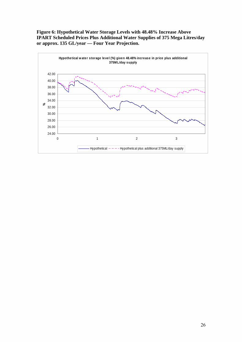
Figure 6: Hypothetical Water Storage Levels with 48.48% Increase Above IPART Scheduled Prices Plus Additional Water Supplies of 375 Mega Litres/day or approx. 135 GL/year — Four Year Projection.

Hypothetical w ater s torage level (%) given 48.48% increase in price plus additional 375ML/day supply

24.00

26.00

28.00

30.00

32.00

34.00

36.00

38.00

40.00

42.00

0 1 2 3

%

Hypothetical Hypothetical plus additional 375ML/day supply

26

End Notes

1. We thank Pham Van Ha and Quyen Nguyen for their valuable research assistance. We are especially grateful to Steve Dowrick and Jack Pezzey for their insightful comments on an earlier version of this paper, and also thank seminar participants at the Crawford School of Economics and Government, The Australian National University on 24 October 2006 and at the Australian Agricultural and Resource Economics Society (AARES) 2006 annual meeting in Sydney on 10 February 2006.

2. We are grateful to Jack Pezzey for this suggestion. For further discussion of how such a system might operate for pollution see Pezzey (2003).

27