SYMBOLIC SOFTWARE FOR SOLITON THEORY: INTEGRABILITY

.

SYMBOLIC SOFTWARE FOR SOLITON THEORY:

INTEGRABILITY, SYMMETRIES

CONSERVATION LAWS

AND EXACT SOLUTIONS

Willy Hereman

Dept. of Mathematical and Computer Sciences

Colorado School of Mines

Golden, Colorado

Kruskal Fest

Symposium in Applied Mathematics:

Nonlinear Waves, Dynamics, Asymtotic Analysis

and Physical Applications

Boulder, Colorado

August 3-6, 1995

I. INTRODUCTION

Symbolic Software

• Painleve test for systems of ODEs and PDEs(Macsyma & Mathematica)

• Conservation laws of systems of evolution equations(Mathematica)

• Solitons via Hirota’s method (Macsyma & Mathematica)

• Lie symmetries for systems of ODEs and PDEs(Macsyma)

Purpose of the programs

• Study of integrability of nonlinear PDEs

• Exact solutions as bench mark for numerical algorithms

• Classification of nonlinear PDEs

• Lie symmetries −→ solutions via reductions

Collaborators

• Unal Goktas, Chris Elmer, Wuning Zhuang(MS students)

• Ameina Nuseir (Ph.D student)

• Mark Coffey (CU-Boulder)

• Tony Miller & Tracy Otto (BS students)

II. SYMBOLIC SOFTWARE

Program 1 – Macsyma

Painleve Integrability Test

for Systems of ODEs and PDEs

Integrability of (a systems of) ODEs or PDEs requires that theonly movable singularities in its solution are poles

Definition: A single equation or system has the PainleveProperty if its solution in the complex plane has no worsesingularities than movable poles

Aim: Verify whether or not the system of equationssatisfies the necessary criteria to have the Painleve Prop-erty

For simplicity, consider the case of a single PDE

The solution f expressed as a Laurent series

f = gα∞∑k=0

ukgk

should only have movable poles

Steps of the Painleve Test

• Step 1:

1. Substitute the leading order term

f ∝ u0 gα

into the given equation

2. Determine the integer α < 0 by balancingthe most singular terms in g

3. Calculate u0

• Step 2:

1. Substitute the generic terms

f ∝ u0 gα + ur g

α+r

into the equation, retaining its most singular terms

2. Require that ur is arbitrary

3. Determine the corresponding values of r > 0called resonances

• Step 3:

1. Substitute the truncated expansion

f = gαR∑k=0

uk gk

into the complete equation(R represents the largest resonance)

2. Determine uk unambiguously at the non-resonance lev-els

3. Check whether or not the compatibilitycondition is satisfied at resonance levels

• An equation or system has the Painleve Property andis conjectured to be integrable if:

1. Step 1 thru 3 can be carried out consistently with α < 0and with positive resonances

2. The compatibility conditions are identicallysatisfied for all resonances

• The above algorithm does not detect essentialsingularities

Painleve Integrability Test

• Painleve test for 3rd order equations by Hajee(Reduce, 1982)

• Painleve program (parts) by Hlavaty (Reduce, 1986)

• ODE Painleve by Winternitz & Rand(Macsyma, 1986)

• PDE Painleve by Hereman & Van den Bulck(Macsyma, 1987)

• Painleve test by Conte & Musette (AMP, 1988)

• Painleve analysis by Renner (Reduce, 1992)

• Painleve test for systems of ODEs and PDEsby Hereman, Elmer and Goktas(Macsyma, 1994-96, under development)

• Painleve test for single ODEs and PDEsby Hereman, Miller and Otto(Mathematica, 1995, under development)

• Painleve test for systems of ODEs and PDEsby Hereman and Miller(Mathematica, 1995-96, planned)

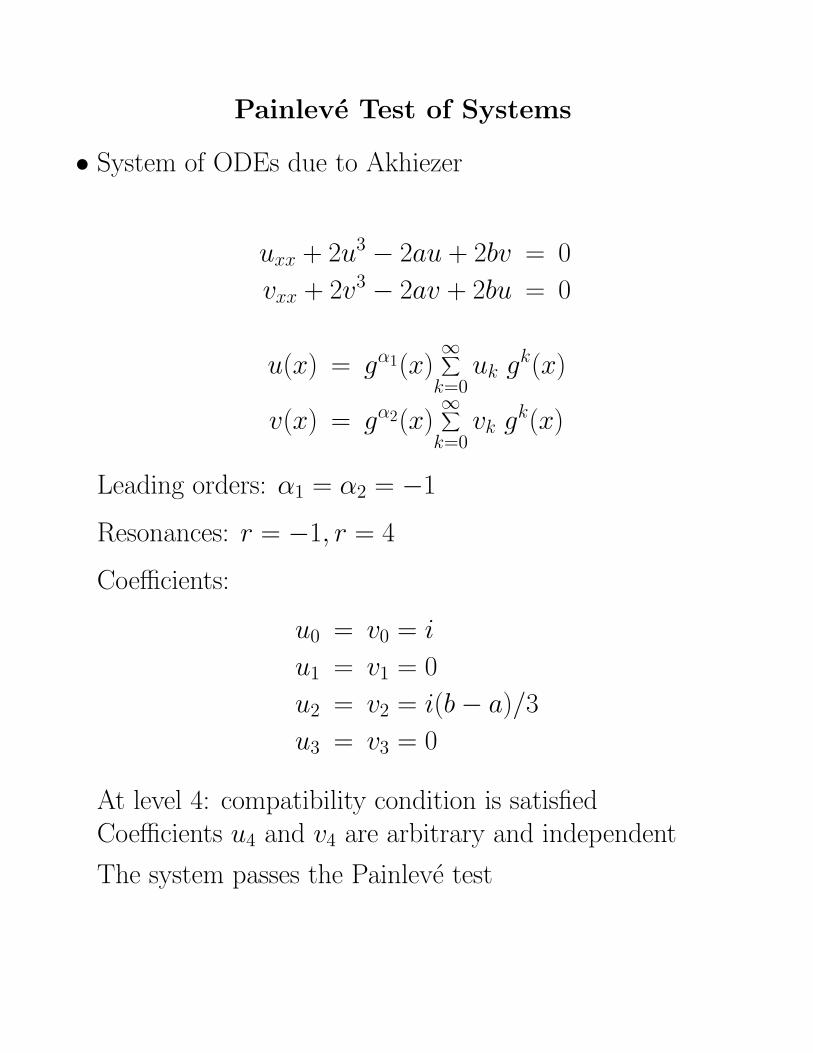
Painleve Test of Systems

• System of ODEs due to Akhiezer

uxx + 2u3 − 2au + 2bv = 0

vxx + 2v3 − 2av + 2bu = 0

u(x) = gα1(x)∞∑k=0

uk gk(x)

v(x) = gα2(x)∞∑k=0

vk gk(x)

Leading orders: α1 = α2 = −1

Resonances: r = −1, r = 4

Coefficients:

u0 = v0 = i

u1 = v1 = 0

u2 = v2 = i(b− a)/3

u3 = v3 = 0

At level 4: compatibility condition is satisfiedCoefficients u4 and v4 are arbitrary and independent

The system passes the Painleve test

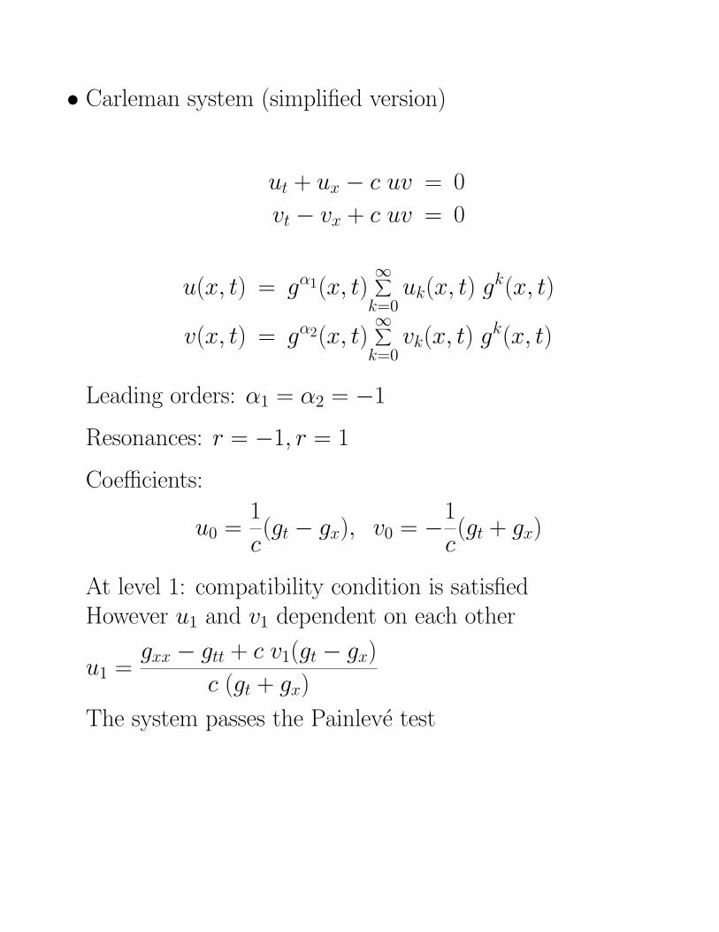
• Carleman system (simplified version)

ut + ux − c uv = 0

vt − vx + c uv = 0

u(x, t) = gα1(x, t)∞∑k=0

uk(x, t) gk(x, t)

v(x, t) = gα2(x, t)∞∑k=0

vk(x, t) gk(x, t)

Leading orders: α1 = α2 = −1

Resonances: r = −1, r = 1

Coefficients:

u0 =1

c(gt − gx), v0 = −1

c(gt + gx)

At level 1: compatibility condition is satisfiedHowever u1 and v1 dependent on each other

u1 =gxx − gtt + c v1(gt − gx)

c (gt + gx)


• Coupled KdV Equations (Hirota-Satsuma system)

ut − 3uux + 6vvx −1

2uxxx = 0

vt + vxxx + 3uvx = 0

Use Kruskal simplification, g(x, t) = x− h(t), in

u(x, t) = gα1(x, t)∞∑k=0

uk(x, t) gk(x, t)

v(x, t) = gα2(x, t)∞∑k=0

vk(x, t) gk(x, t)

Leading orders: First Branch α1 = α2 = −2

Resonances: r = −2,−1, 3, 4, 6, 8

Coefficients:

u0 = −4, v0 = −2

u1 = v1 = 0

u2 = ht/3, v2 = 2ht/3

u5 = −htt + 30v3ht63

, v5 =htt − 12v3ht

63

u7 = −v4t + 12v3v4

12, v7 =

4hthtt + v3(8h2t − 84v4) + 21v4t

504

At level 3: compatibility condition is satisfiedHere u3 = v3 , one function is arbitary

At level 4: compatibility condition is satisfiedHere u4 = 2v4, one function is arbitrary

At level 6: compatibility condition is satisfied

Here u6 =−v3t + 24v6 − 3v3

2

12,

one function is arbitrary


Here u8 =

−httt + 6v3htt + (12v3t + 198v23)ht − 3024v8 − 756v4

2

756,


Leading orders: Second Branch α1 = −2, α2 = −1

Resonances: r = −1, 0, 1, 4, 5, 6

Coefficients:

u0 = −2, v0 free

u1 = 0, v1 free

u2 = −(2ht + 3v20)/6, v2 = (4v0ht + 3v3

0)/12

u3 = −v0v1, v3 =v0t + 3v2

0v1

12

At level 0: compatibility condition is satisfiedCoefficient v0 is arbitary

At level 1: compatibility condition is satisfiedCoefficient v1 is arbitary


Here u4 = −16v0h2t + 24v3

0ht − 24v1t + 9v50 + 72u4v0

288,



Here

u5 =2htt − 12v0v1ht + 3v0v0t − 9v0

3v1

18one function is arbitrary


Here

u6 =1

5760(−64v0h

3t− 144v3

0h2t +(96v1t− 108v5

0− 480u4v0)ht

+24v02v1t− 16v0tt+ 288v3

0v21− 27v7

0− 360u4v30+ 576u6v0)



Program 2 – Mathematica

Conserved Densities

• Purpose

Compute polynomial-type conservation laws ofsingle evolution equations and systems of evolution equa-tions

For simplicity, consider a single evolution equation

ut = F(u, ux, uxx, ..., unx)

Conservation law is of the form

ρt + Jx = 0

both ρ(u, ux, u2x, . . . , unx) and J(u, ux, u2x, . . . , unx)are polynomials in their arguments

Consequently

P =∫ +∞−∞ ρ dx = constant

provided J vanishes at infinity

– Conservation laws describe the conservation offundamental physical quantities such as mass,linear momentum, total energy (compare with constantsof motion in mechanics)

– For nonlinear PDEs, the existence of a sufficiently large(in principal infinite) number of conservation laws as-sures complete integrability

– Tool to test numerical integrators for PDEs

• Example

Consider the KdV equation, ut + uux + u3x = 0Conserved densities:

ρ1 = u

ρ2 = u2

ρ3 = u3 − 3u2x

...

ρ6 = u6 − 60u3u2x − 30u4

x + 108u2u22x

+720

7u3

2x −648

7uu2

3x +216

7u2

4x

...

Integrable equations have ∞ many conservation laws

• Algorithm and Implementation

Consider the scaling (weights) of the KdV

u ∼ ∂2

∂x2,

∂

∂t∼ ∂3

∂x3

Compute building blocks of ρ3

(i) Start with building block u3

Divide by u and differentiate twice (u2)2x

Produces the list of terms

[u2x, uu2x] −→ [u2

x]

Second list: remove terms that are total derivativewith respect to x or total derivativeup to terms earlier in the list

Divide by u2 and differentiate twice (u)4x

Produces the list: [u4x] −→ [ ]

[ ] is the empty list

Gather the terms:

ρ3 = u3 + c[1]u2x

where the constant c1 must be determined

(ii) Compute∂ρ3

∂t= 3u2ut + 2c1uxuxt

Replace ut by −(uux + uxxx) and uxt by −(uux + uxxx)x

(iii) Integrate the result with respect to x

Carry out all integrations by parts

∂ρ3

∂t=−[

3

4u4 + (c1−3)uu2

x + 3u2uxx− c1u2xx+ 2c1uxuxxx]x

−(c1 + 3)u3x

The last non-integrable term must vanish

Thus, c1 = −3

Result:ρ3 = u3 − 3u2

x

(iv) Expression [. . .] yields

J3 =3

4u4 − 6uu2

x + 3u2uxx + 3u2xx − 6uxuxxx

Computer building blocks of ρ6

(i) Start with u6

Divide by u and differentiate twice

(u5)2x produces the list of terms

[u3u2x, u

4u2x] −→ [u3u2x]

Next, divide u6 by u2, and compute (u4)4x

Corresponding list:

[u4x, uu

2xu2x, u

2u22x, u

2uxu3x, u3u4x] −→ [u4

x, u2u2

2x]

Proceed with (u6

u3)6x = (u3)6x, (u6

u4)8x = (u2)8x

and (u6

u5)10x = (u)10x

Obtain the lists:

[u32x, uxu2xu3x, uu

23x, u

2xu4x, uu2xu4x, uuxu5x, u

2u6x] −→[u3

2x, uu23x]

[u24x, u3xu5x, u2xu6x, uxu7x, uu8x] −→ [u2

4x]

and [u10x] −→ [ ]

Gather the terms:

ρ6 = u6 + c1u3u2

x+ c2u4x+ c3u

2u22x+ c4u

32x+ c5uu

23x+ c6u

24x

where the constants ci must be determined

(ii) Compute ∂∂tρ6

Replace ut, uxt, . . . , unx,t by −(uux + uxxx), . . .

(iii) Integrate the result with respect to x

Carry out all integrations by parts

Require that non-integrabe part vanishes

Set to zero all the coefficients of the independentcombinations involving powers of u andits derivatives with respect to x

Solve the linear system for unknowns c1, c2, . . . , c6

Result:

ρ6 = u6 − 60u3u2x − 30u4

x + 108u2u22x

+720

7u3

2x −648

7uu2

3x +216

7u2

4x

(iv) Flux J6 can be computed by substitutingthe constants into the integrable part of ρ6

Conserved Densities

• Conserved densities by Ito & Kako(Reduce, 1985, 1994)

• Conserved densities in DELiA by Bocharov(Pascal, 1990)

• Conserved densities by Gerdt (Reduce, 1993)

• Conserved densities by Roelofs, Sanders and Wang(Reduce 1994, Maple 1995)

• Conserved densities by Hereman and Goktas(Mathematica, 1993-1995)

• Conservation laws by Wolf (Reduce, 1995)

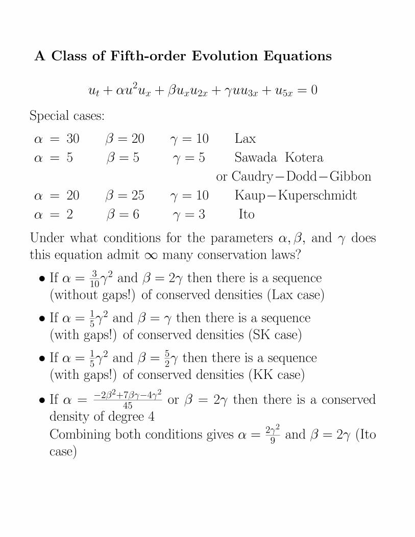
A Class of Fifth-order Evolution Equations

ut + αu2ux + βuxu2x + γuu3x + u5x = 0

Special cases:

α = 30 β = 20 γ = 10 Lax

α = 5 β = 5 γ = 5 Sawada Kotera

or Caudry−Dodd−Gibbon

α = 20 β = 25 γ = 10 Kaup−Kuperschmidt

α = 2 β = 6 γ = 3 Ito

Under what conditions for the parameters α, β, and γ doesthis equation admit ∞ many conservation laws?

• If α = 310γ

2 and β = 2γ then there is a sequence(without gaps!) of conserved densities (Lax case)

• If α = 15γ

2 and β = γ then there is a sequence(with gaps!) of conserved densities (SK case)

• If α = 15γ

2 and β = 52γ then there is a sequence

(with gaps!) of conserved densities (KK case)

• If α = −2β2+7βγ−4γ2

45 or β = 2γ then there is a conserveddensity of degree 4

Combining both conditions gives α = 2γ2

9 and β = 2γ (Itocase)

Conserved Densities of Systems of Evolution Eqs.

• Coupled KdV Equations (Hirota-Satsuma system)

ut − a(uxxx + 6uux)− 2bvvx = 0

vt + vxxx + 3uvx = 0

u ∼ ∂2

∂x2, v ∼ ∂2

∂x2

ρ1 = u

ρ2 = u2 +2

3bv2

ρ3 = (1 + a)(u3 − 1

2u2x) + b(uv2 − v2

x)

and e.g.

ρ4 = u4 − 2uu2x +

1

5u2xx

+4

5b(u2v2 +

2

3uvvxx +

8

3uv2

x −2

3v2xx) +

4

15b2v4

provided a = 12

There are infinitely many more conservation laws

• The Ito system

ut − uxxx − 6uux − 2vvx = 0

vt − 2uxv − 2uvx = 0

u ∼ ∂2

∂x2, v ∼ ∂2

∂x2

ρ1 = c1u + c2v

ρ2 = u2 + v2

ρ3 = 2u3 + 2uv2 − u2x

ρ4 = 5u4 + 6u2v2 + v4 − 10uu2x + 2v2u2x + u2

2x

and there are infinitely many more conservation laws

• The Drinfel’d-Sokolov system

ut + 3vvx = 0

vt + vux + 2uvx + 2v3x = 0

u ∼ ∂2

∂x2, v free, choose v ∼ ∂2

∂x2

ρ1 = u

ρ2 = v2

ρ3 =−2

9u3 + uv2 +

1

6u2x −

3

2v2x

ρ4 =1

2u4 − 1

6u2v2 − 1

8v4 − 1

6uu2

x + uv2x

− 5

12v2u2x +

1

36u2

2x −3

4v2

2x

and there are presumably infinitely many moreconservation laws

• The dispersiveless long-wave system

ut + vux + uvx = 0

vt + ux + vvx = 0

u free, v free, but u ∼ 2v

choose u ∼ ∂

∂xand 2v ∼ ∂

∂x

ρ1 = v

ρ2 = u

ρ3 = uv

ρ4 = u2 + uv2

ρ5 = 3u2v + uv3

ρ6 =1

3u3 + u2v2 +

1

6uv4

ρ7 = u3v + u2v3 +1

10uv5

ρ8 =1

3u4 + 2u3v2 + u2v4 +

1

15uv6

always the same set irrespective the choice of weights

Further Examples

• A generalized Schamel equation

n2ut + (n + 1)(n + 2)u2nux + uxxx = 0

n positive integer

ρ1 = u, ρ2 = u2

ρ3 =1

2u2x −

n2

2u2+2

n

no further conservation laws

• The Boussinesq equation

utt − buxx + 3uuxx + 3u2x + au4x = 0

a and b are real constants

Write as system of evolution equations

ut + vx = 0

vt + bux − 3uux − au3x = 0

u ∼ ∂2

∂x2, b ∼ ∂2

∂x2, v free, take v ∼ ∂3

∂x3

ρ1 = u

ρ2 = u

ρ3 = bu

ρ4 = bc1u + c2uv

ρ5 = b2c1u + c2(bu2 − u3 + v2 + au2

x)

and there are infinitely many more conservation laws

• A modified vector derivative NLS equation

∂B⊥

∂t+

∂

∂x(B2

⊥B⊥) + αB⊥0B⊥0 ·∂B⊥

∂x+ ex ×

∂2B⊥

∂x2= 0

Replace vector equation by

ut +(u(u2 + v2) + βu− vx

)x

= 0

vt +(v(u2 + v2) + ux

)x

= 0

u and v denote the components of B⊥ paralleland perpendicular to B⊥0 and β = αB2

⊥0

2u ∼ ∂

∂x, 2v ∼ ∂

∂x, β ∼ ∂

∂x

The first 6 conserved densities are:

ρ1 = c1u + c2v

ρ2 = u2 + v2

ρ3 =1

2(u2 + v2)2 − uvx + uxv + βu2

ρ4 =1

4(u2 + v2)3 +

1

2(u2

x + v2x)− u3vx + v3ux +

β

4(u4 − v4)

ρ5 =1

4(u2 + v2)4 − 2

5(uxvxx − uxxvx) +

4

5(uux + vvx)

2

+6

5(u2 + v2)(u2

x + v2x)− (u2 + v2)2(uvx − uxv)

+β

5(2u2

x − 4u3vx + 2u6 + 3u4v2 − v6) +β2

5u4

ρ6 =7

16(u2 + v2)5+

1

2(u2

xx + v2xx)

− 5

2(u2 + v2)(uxvxx−uxxvx) + 5(u2 + v2)(uux + vvx)

2

+15

4(u2 + v2)2(u2

x + v2x)−

35

16(u2 + v2)3(uvx − uxv)

+β

8(5u8 + 10u6v2 − 10u2v6 − 5v8 + 20u2u2

x

− 12u5vx + 60uv4vx − 20v2v2x)

+β2

4(u6 + v6)

Table 1 Conserved Densities for Sawada-Kotera and Lax equations

Density Sawada-Kotera equation Lax equation

ρ1 u u

ρ2 ---- 12u2

ρ313u3 − u2

x13u3 − 1

6u2x

ρ414u4 − 9

4uu2x + 3

4u22x

14u4 − 1

2uu2x + 1

20u22x

ρ6 ---- 15u5 − u2u2

x + 15uu2

2x − 170u2

3x

ρ616u6 − 25

4 u3u2x − 17

8 u4x + 6u2u2

2x16u6 − 5

3u3u2x − 5

36u4x + 1

2u2u22x

+2u32x − 21

8 uu23x + 3

8u24x + 5

63u32x − 1

14uu23x + 1

252u24x

ρ717u7 − 9u4u2

x − 545 uu4

x + 575 u3u2

2x17u7 − 5

2u4u2x − 5

6uu4x + u3u2

2x

+64835 u2

xu22x + 489

35 uu32x − 261

35 u2u23x +1

2u2xu2

2x + 1021uu3

2x − 314u2u2

3x

−28835 u2xu2

3x + 8135uu2

4x − 935u2

5x − 542u2xu2

3x + 142uu2

4x − 1924u2

5x

ρ8 ---- 18u8 − 7

2u5u2x − 35

12u2u4x + 7

4u4u22x

+72uu2

xu22x + 5

3u2u32x + 7

24u42x + 1

2u3u23x

−14u2

xu23x − 5

6uu2xu23x + 1

12u2u24x

+ 7132u2xu2

4x − 1132uu2

5x + 13432u2

6x

Table 2 Conserved Densities for Kaup-Kuperschmidt and Ito equations

Density Kaup-Kuperschmidt equation Ito equation

ρ1 u u

ρ2 ---- u2

2

ρ3u3

3 − 18u2

x ----

ρ4u4

4 − 916uu2

x + 364u2

2xu4

4 − 94uu2

x + 34u2

2x

ρ5 ---- ----

ρ6u6

6 − 3516u3u2

x − 31256u4

x + 5164u2u2

2x ----

+ 37256u3

2x − 15128uu2

3x + 3512u2

4x

ρ7u7

7 − 278 u4u2

x − 369320uu4

x + 6940u3u2

2x ----

+26194480u2

xu22x + 2211

2240uu32x − 477

1120u2u23x

−171640u2xu2

3x + 27560uu2

4x − 94480u2

5x

ρ8 ---- ----

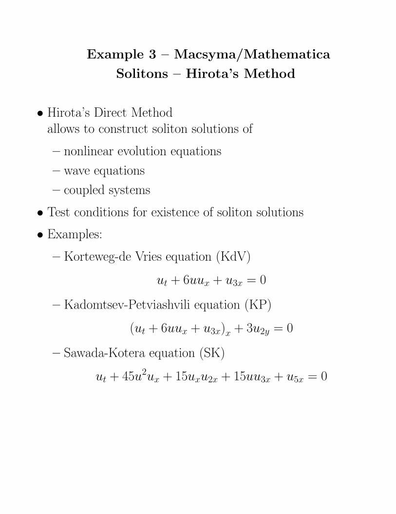
Example 3 – Macsyma/Mathematica

Solitons – Hirota’s Method

• Hirota’s Direct Methodallows to construct soliton solutions of

– nonlinear evolution equations

– wave equations

– coupled systems

• Test conditions for existence of soliton solutions

• Examples:

– Korteweg-de Vries equation (KdV)

ut + 6uux + u3x = 0

– Kadomtsev-Petviashvili equation (KP)

(ut + 6uux + u3x)x + 3u2y = 0

– Sawada-Kotera equation (SK)

ut + 45u2ux + 15uxu2x + 15uu3x + u5x = 0

Hirota’s Method

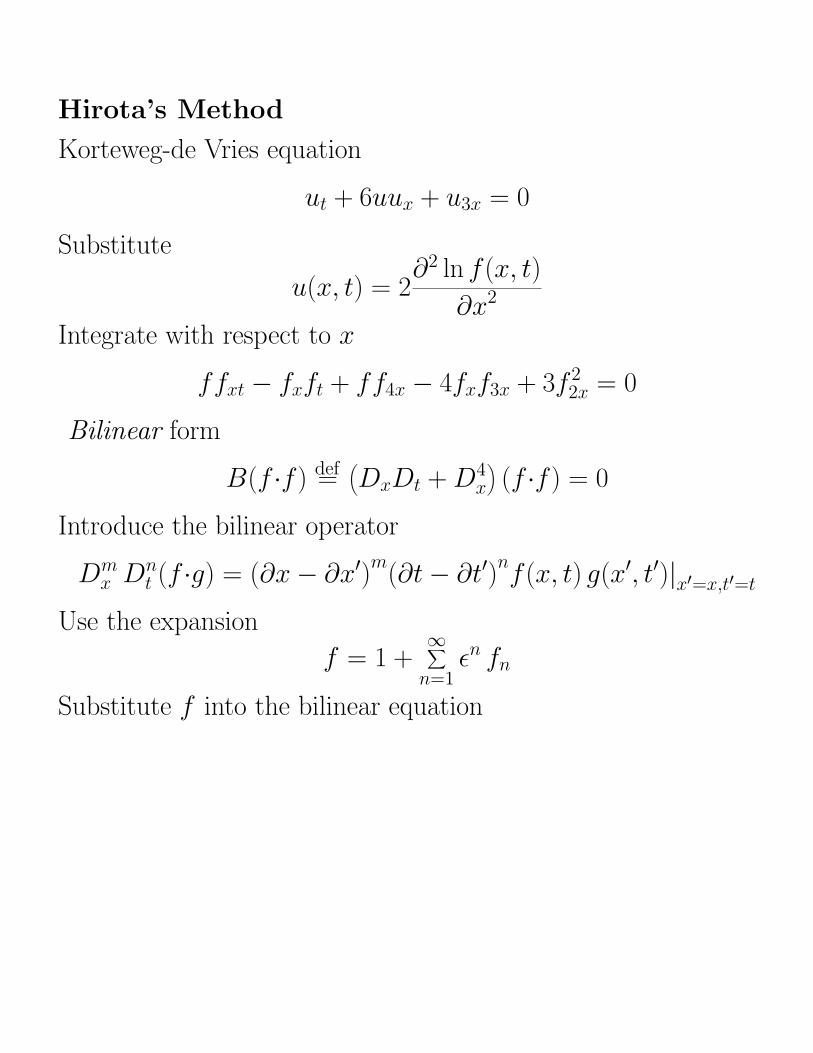
Korteweg-de Vries equation

ut + 6uux + u3x = 0

Substitute

u(x, t) = 2∂2 ln f (x, t)

∂x2

Integrate with respect to x

ffxt − fxft + ff4x − 4fxf3x + 3f 22x = 0

Bilinear form

B(f ·f ) def=(DxDt +D4

x

)(f ·f ) = 0

Introduce the bilinear operator

Dmx D

nt (f ·g) = (∂x− ∂x′)

m(∂t− ∂t′)

nf (x, t) g(x′, t′)|x′=x,t′=t

Use the expansion

f = 1 +∞∑n=1

εn fn

Substitute f into the bilinear equation

Collect powers in ε (book keeping parameter)

O(ε0) : B(1·1) = 0

O(ε1) : B(1·f1 + f1·1) = 0

O(ε2) : B(1·f2 + f1·f1 + f2·1) = 0

O(ε3) : B(1·f3 + f1·f2 + f2·f1 + f3·1) = 0

O(ε4) : B(1·f4 + f1·f3 + f2·f2 + f3·f1 + f4·1) = 0

O(εn) : B(n∑j=0

fj·fn−j) = 0 with f0 = 1

Start with

f1 =N∑i=1

exp(θi) =N∑i=1

exp (ki x− ωi t + δi)

ki, ωi and δi are constantsDispersion law

ωi = k3i (i = 1, 2, ..., N)

If the original PDE admits a N-soliton solutionthen the expansion will truncate at level n = N

Consider the case N=3Terms generated by B(f1, f1) determine

f2 = a12 exp(θ1 + θ2) + a13 exp(θ1 + θ3) + a23 exp(θ2 + θ3)

= a12 exp [(k1 + k2)x− (ω1 + ω2) t + (δ1 + δ2)]

+ a13 exp [(k1 + k3)x− (ω1 + ω3) t + (δ1 + δ3)]

+ a23 exp [(k2 + k3)x− (ω2 + ω3) t + (δ2 + δ3)]

Calculate the constants a12, a13 and a23

aij =(ki − kj)

2

(ki + kj)2 i, j = 1, 2, 3

Terms from B(f1·f2 + f2·f1) determine

f3 = b123 exp(θ1 + θ2 + θ3)

= b123 exp [(k1+k2+k3)x−(ω1+ω2+ω3)t+(δ1+δ2+δ3)]

with

b123 = a12 a13 a23 =(k1 − k2)

2 (k1 − k3)2 (k2 − k3)

2

(k1 + k2)2 (k1 + k3)

2 (k2 + k3)2

Subsequently, fi = 0 for i > 3

Set ε = 1

f = 1 + exp θ1 + exp θ2 + exp θ3

+ a12 exp(θ1 + θ2) + a13 exp(θ1 + θ3) + a23 exp(θ2 + θ3)

+ b123 exp(θ1 + θ2 + θ3)

Return to the original u(x, t)

u(x, t) = 2∂2 ln f (x, t)

∂x2

Single soliton solution

f = 1 + eθ , θ = kx− ωt + δ

k, ω and δ are constants and ω = k3

Substituting f into

u(x, t) = 2∂2 ln f (x, t)

∂x2

= 2(fxxf − f 2

x

f 2)

Take k = 2K

u = 2K2sech2K(x− 4K2t + δ)

Two-soliton solution

f = 1 + eθ1 + eθ2 + a12eθ1+θ2

θi = kix− ωit + δi

with ωi = k3i , (i = 1, 2) and a12 = (k1−k2)

2

(k1+k2)2

Select

eδi =c2ikiekix−ωit+∆i

f =1

4fe−

12(θ1+θ2)

θi = kix− ωit + ∆i

c2i =k2 + k1

k2 − k1

kiReturn to u(x, t)

u(x, t) = u(x, t) = 2∂2 ln f (x, t)

∂x2

=

k22 − k2

1

2

k2

2cosech2 θ22 + k2

1sech2 θ1

2

(k2 coth θ22 − k1 tanh θ1

2 )2

Program 4 – MacsymaLie-point Symmetries

• System of m differential equations of order k

∆i(x, u(k)) = 0, i = 1, 2, ...,m

with p independent and q dependent variables

x = (x1, x2, ..., xp) ∈ IRp

u = (u1, u2, ..., uq) ∈ IRq

• The group transformations have the form

x = Λgroup(x, u), u = Ωgroup(x, u)

where the functions Λgroup and Ωgroup are to be determined

• Look for the Lie algebra L realized by the vector field

α =p∑i=1ηi(x, u)

∂

∂xi+

q∑l=1ϕl(x, u)

∂

∂ul

Procedure for finding the coefficients

• Construct the kth prolongation pr(k)α of the vector field α

• Apply it to the system of equations

• Request that the resulting expression vanisheson the solution set of the given system

pr(k)α∆i |∆j=0 i, j = 1, ...,m

• This results in a system of linear homogeneous PDEsfor ηi and ϕl, with independent variables x and u( determining equations)

• Procedure thus consists of two major steps:

deriving the determining equationssolving the determining equations

Procedure for Computing the Determining Equations

• Use multi-index notation J = (j1, j2, ..., jp) ∈ INp,to denote partial derivatives of ul

ulJ ≡∂|J |ul

∂x1j1∂x2

j2...∂xpjp,

where |J | = j1 + j2 + ... + jp

• u(k) denotes a vector whose components are all the partialderivatives of order 0 up to k of all the ul

• Steps:

(1) Construct the kth prolongation of the vector field

pr(k)α = α +q∑l=1

∑JψJl (x, u(k))

∂

∂ulJ, 1 ≤ |J | ≤ k

The coefficients ψJl of the first prolongation are:

ψJil = Diϕl(x, u)−p∑j=1

ulJjDiηj(x, u),

where Ji is a p−tuple with 1 on the ith position and zeroselsewhere

Di is the total derivative operator

Di =∂

∂xi+

q∑l=1

∑JulJ+Ji

∂

∂ulJ, 0 ≤ |J | ≤ k

Higher order prolongations are defined recursively:

ψJ+Jil = Diψ

Jl −

p∑j=1

ulJ+JjDiη

j(x, u), |J | ≥ 1

(2) Apply the prolonged operator pr(k)α to eachequation ∆i(x, u(k)) = 0

Require that pr(k)α vanishes on the solution set of the sys-tem

pr(k)α ∆i |∆j=0 = 0 i, j = 1, ...,m

(3) Choose m components of the vector u(k),say v1, ..., vm, such that:

(a) Each vi is equal to a derivative of a ul (l = 1, ..., q)with respect to at least one variable xi (i = 1, ..., p).

(b) None of the vi is the derivative of another one in theset.

(c) The system can be solved algebraically for the vi interms of the remaining components of u(k), which we de-noted by w:

vi = Si(x,w), i = 1, ...,m.

(d) The derivatives of vi,

viJ = DJSi(x,w),

where DJ ≡ Dj11 D

j22 ...D

jpp , can all be expressed in terms

of the components of w and their derivatives, without everreintroducing the vi or their derivatives.

For instance, for a system of evolution equations

uit(x1, ..., xp−1, t) = F i(x1, ..., xp−1, t, u(k)), i = 1, ...,m,

where u(k) involves derivatives with respect to the variablesxi but not t, choose vi = uit.

(4) Eliminate all vi and their derivatives from the ex-pression prolonged vector field, so that all the remainingvariables are independent

(5) Obtain the determining equations for ηi(x, u) andϕl(x, u) by equating to zero the coefficients of the remain-ing independent derivatives ulJ .

Example: The Korteweg-de Vries Equation

ut + auux + uxxx = 0

• one equation (parameter a)

• two independent variables t and x

• one dependent variable u

• vector field α = ηx ∂∂x + ηt ∂∂t + ϕu ∂∂u

Format for SYMMGRP.MAX

• variables x[1] = x, x[2] = t, u[1] = u

• equation e1 : u[1, [0, 1]] + a ∗ u[1] ∗ u[1, [1, 0]] + u[1, [3, 0]]

• variable to be eliminated v1 : u[1, [0, 1]]

• coefficients of vectorfield in SYMMGRP.MAX:eta[1] = ηx, eta[2] = ηt and phi[1] = ϕu

There are only eight determining equations

∂eta[2]

∂u[1]= 0

∂eta[2]

∂x[1]= 0

∂eta[1]

∂u[1]= 0

∂2phi[1]

∂u[1]2= 0

∂2phi[1]

∂u[1]∂x[1]− ∂2eta[1]

∂x[1]2= 0

∂phi[1]

∂x[2]+∂3phi[1]

∂x[1]3+ u[1]

∂phi[1]

∂x[1]= 0

3∂3phi[1]

∂u[1]∂x[1]2− ∂eta[1]

∂x[2]− ∂3eta[1]

∂x[1]3

+ 2 u[1]eta[1]

∂x[1]+ phi[1] = 0

u[1]∂eta[2]

∂x[2]+ 3

∂3phi[1]

∂u[1]∂x[1]2− ∂eta[1]

∂x[2]− ∂3eta[1]

∂x[1]3

− u[1]eta[1]

∂x[1]+ phi[1] = 0

The solution in the original variables

ηx = k1 + k3 t− k4 x

ηt = k2 − 3k4 t

ϕu = k3 + 2 k4 u

The four infinitesimal generators are

G1 = ∂xG2 = ∂tG3 = t ∂x + ∂uG4 = x ∂x + 3 t ∂t − 2 u ∂u

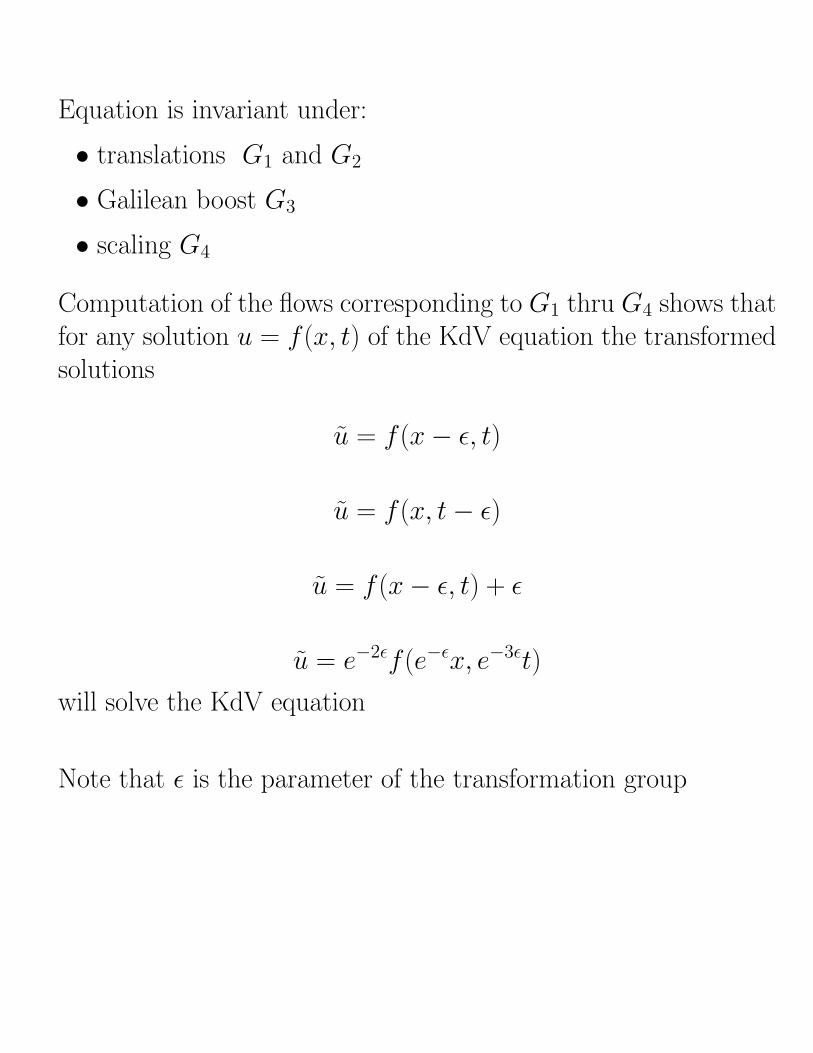
Equation is invariant under:

• translations G1 and G2

• Galilean boost G3

• scaling G4

Computation of the flows corresponding to G1 thru G4 shows thatfor any solution u = f (x, t) of the KdV equation the transformedsolutions

u = f (x− ε, t)

u = f (x, t− ε)

u = f (x− ε, t) + ε

u = e−2εf (e−εx, e−3εt)

will solve the KdV equation

Note that ε is the parameter of the transformation group

III. PLANS FOR THE FUTURE

Extension of Symbolic Software Packages(Macsyma/Mathematica)

• Lie symmetries of differential-difference equations

• Solver for systems of linear, homogeneous PDEs(Hereman)

• Painleve test for systems of PDEs(Elmer, Goktas & Coffey)

• Solitons via Hirota’s method for bilinear equations (Zhuang)

• Simplification of Hirota’s method (Hereman & Nuseir)

• Conservation laws of PDEs with variable coefficients (Goktas)

• Lax pairs, special solutions, ...

New Software

• Wavelets (prototype/educational tool)

• Other methods for Differential Equations

Documents

SYMBOLIC SOFTWARE FOR SOLITON THEORY: INTEGRABILITY