Symmetry principles and nuclear structure

Progress in Particle and Nuclear Physics 59 (2007) 337–354www.elsevier.com/locate/ppnp

Review

Symmetry principles and nuclear structure

J. Jolie

Institut fur Kernphysik, University of Cologne, Germany

Abstract

We review the use of dynamical symmetries in nuclear physics using the interacting boson model.Special emphasis is made on experimental signatures of these symmetries. We illustrate this by a detailedstudy on mixed symmetry states in 94Mo.c© 2007 Elsevier B.V. All rights reserved.

Keywords: Interacting Boson Model; Dynamical symmetries; Collective excitations

1. Introduction

The atomic nucleus is formed by an amalgam of a finite number of nucleons, the protons andneutrons, which interact by all of the four fundamental forces. Moreover, due to its small size,some millionth of a billionth of a meter, the atomic nucleus forms a pure quantum mechanicalsystem. To understand the quantal world at work in the atomic nucleus, powerful theoretical toolsare needed.

A very important one is symmetry, a mathematical concept that has its basis in commonsense. Suppose one has an isolated physical system which does not interact with the outside,it is then logical that the physical laws governing this system are independent of how wedefine a coordinate system or at which time we study the system. The laws should be invariantwith respect to certain transformations of our coordinates. This simple statement leads to threefundamental conservation laws which greatly simplify our description of nature: conservationof energy, linear momentum and angular momentum. On these three benchmarks classicalmechanics was built. These quantities are also conserved in isolated quantal systems, along witha particular behavior for energy and linear momentum described by the Heisenberg uncertainty

E-mail address: [email protected].

0146-6410/$ - see front matter c© 2007 Elsevier B.V. All rights reserved.doi:10.1016/j.ppnp.2006.12.023

http://www.elsevier.com/locate/ppnp

mailto:[email protected]

http://dx.doi.org/10.1016/j.ppnp.2006.12.023

338 J. Jolie / Progress in Particle and Nuclear Physics 59 (2007) 337–354

relations. In many cases an additional reflection symmetry applies yielding another conservedquantity called parity. In particular, low-lying excitations of atomic nuclei can be classified byenergy E , spin and parity Jπ , and the 2J + 1 possible values of the magnetic projection M .

Are there other conserved quantities that permit us to simplify the description of a complicatedquantal system? Niels Bohr touched upon a new kind of symmetry when he solved the hydrogenproblem. He obtained a very simple expression involving the principal quantum number n.The energies of excited states of the hydrogen atom are inversely proportional to the squareof n. What underlies this simple relationship is the presence of a dynamical symmetry. Thesesymmetries, connected to the equations describing the dynamics of the quantal system, lead toconserved quantities denoted by quantum numbers such as the principal quantum number n.In 1935 Vladimir Fock showed that the equations governing the motion of an electron aroundan atomic nucleus conserved orthogonal transformations in four dimensions, described by theSO(4) group. The hydrogen atom has an SO(4) dynamical symmetry. Group theory then gavethe possible values of the quantum numbers and explained the observed n2 degeneracy of stateswhen neglecting electron spin.

Dynamical symmetries turned out to be particularly useful in nuclear physics after FrancescoIachello (Groningen) and Akito Arima (Tokyo) proposed an extremely simple and elegantInteracting Boson Model to describe the dynamics of excited heavy atomic nuclei [1]. This modelcombined ingredients of the two most successful models used to describe atomic nuclei in themid-seventies: the nuclear shell model and the collective model. The shell model considers theatomic nucleus as an ensemble of weakly interacting fermions, the neutrons and protons. Theyoccupy single-particle orbits with spin j , which can only contain 2 j + 1 identical nucleons,leading to a shell structure. So-called closed-shell nuclei show great stability and allow one toneglect most nucleons for the description of low-lying excitations in heavier nuclei. Despitethis truncation in heavy nuclei away from the closed shells, many shell model orbits have tobe considered, making calculations prohibitively complex even with modern computers. Thecollective model solves this problem by taking a different approach. Heavy nuclei, formed bysome hundred nucleons, can be considered as a droplet of a quantum liquid. The excitationsof such a droplet are then formed by vibrations and rotations much like a molecule vibratingand rotating. When applied to the simplest systems, even–even nuclei with an even number ofprotons and neutrons, the basic constituents of the model, the surface vibrations, are bosons. Thecollective model has been extremely successful in describing certain classes of nuclei away fromclosed shells [2].

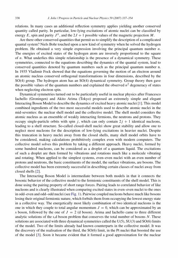
The Interacting Boson Model is intermediate between both models in that it connects thebosonic behavior of the collective model to the fermionic constituents of the shell model. This isdone using the pairing property of short range forces. Pairing leads to correlated behavior of likenucleons and is clearly illustrated when comparing excited states in even–even nuclei to the onesin odd–even and odd–odd nuclei (see Fig. 1). Pairwise coupled nucleons behave much like bosonslosing their original fermionic nature, which forbids them from occupying the lowest energy statein a collective way. The energetically most likely combination of two identical nucleons is theone in which they couple to total angular momentum J = 0, which can be approximated by ans boson, followed by the one of J = 2 (d boson). Arima and Iachello came to three differentanalytic solutions of the s,d boson problem that conserves the total number of bosons N . Thesesolutions are associated with three dynamical symmetries called the U(5), SU(3) and SO(6) limitsof the model. Two of the limits already had known counterparts in the collective model. It wasthe discovery of the realisation of the third, the SO(6) limit, in the Pt nuclei that boosted the useof the model [3]. Soon it became evident that it formed a good approximation for the nuclear

J. Jolie / Progress in Particle and Nuclear Physics 59 (2007) 337–354 339

Fig. 1. Schematic figure showing the importance of pairing when comparing the level densities of even–even, odd-A andodd–odd nuclei.

Fig. 2. On the left the hydrogen atom and its associated quantum numbers. On the right the excited level scheme of112Cd classified according to the quantum numbers of the U(5) limit.

many-body problem in many nuclei. Fig. 2 compares the dynamical symmetries observed in theatomic nucleus with the hydrogen atom. A detailed inspection shows that those observed in thenucleus are less exact than those of the atom. The reason is that in the nucleus many particlesstrongly interact by a complex force, while in the atom the electrons are generally well separatedand the Coulomb force is simple to treat.

This lecture is structured as follows. Section 2 introduces the general concept of dynamicalsymmetries, which is then applied in Section 3 to the s,d boson problem. In Section 4 we reviewsome more advanced topics illustrating the power of symmetry approaches. Finally, in Section 5we give our conclusions.

2. Dynamical symmetries

Before introducing the interacting Boson Model, we review the basic mathematical featuresof symmetries and dynamical symmetries. Hereby the connection to the quantum mechanicaldescription of nature will be outlined.

A hamiltonian H which commutes with the generators gi that form a Lie algebra G, that is,

∀gi ∈ G : [H , gi ] = 0, (1)


is said to have a symmetry G or, alternatively, to be invariant under G. The construction ofCasimir operators which satisfy the commutation property (1) is explained in detail in manytextbooks, e.g. [4].

The determination of operators gi that leave invariant the hamiltonian of a given physicalsystem is central to any quantum-mechanical description. In this way the classical notion of aconserved quantity is transcribed in quantum mechanics into the form of the symmetry property(1) of the hamiltonian.

A well-known consequence of a symmetry is the occurrence of degeneracies in theeigenspectrum of H . Given an eigenstate |γ 〉 of H with energy E , condition (1) implies thatthe states gi |γ 〉 all have the same energy:

H gi |γ 〉 = gi H |γ 〉 = Egi |γ 〉. (2)

An arbitrary eigenstate of H shall be written as |Γγ 〉, where the first quantum number Γ isdifferent for states with different energies and the second quantum number γ is needed to labeldegenerate eigenstates. The eigenvalues of a hamiltonian that satisfies (1) depend on Γ only,

H |Γγ 〉 = E(Γ )|Γγ 〉, (3)

and, furthermore, the transformations gi do not admix states with different Γ :

gi |Γγ 〉 =

∑γ ′

aΓγ ′γ (i)|Γγ ′

〉. (4)

This simple discussion of the consequences of a hamiltonian symmetry illustrates at once therelevance of group theory in quantum mechanics. Symmetry implies degeneracy and eigenstatesthat are degenerate in energy provide a Hilbert space in which irreducible representations of thesymmetry group are constructed. Consequently, the irreducible representations of a given groupdirectly determine the degeneracy structure of a hamiltonian with the symmetry associated tothat group.

The fact that degenerate eigenstates correspond to the so-called irreducible representationsΓγ ′ shall be taken for granted here but it can, in fact, be justified on fundamentalgrounds (Wigner’s principle). The principle states that the Hilbert space of degenerateeigenstates provides an irreducible representation of the complete symmetry of the hamiltonian.Consequently, an observed degeneracy is either accidental in which case it would disappearby increasing the precision of measurement, or it is the result of a hidden symmetry of thehamiltonian.

Because of Wigner’s principle eigenstates of H can be denoted as |Γγ 〉 where the symbol Γlabels the irreducible representations of G. Note that the same irreducible representation mightoccur more than once in the eigenspectrum of H and, therefore, an additional multiplicity labelη should be introduced to define a complete labelling of eigenstates as |ηΓγ 〉.

A sufficient condition for a hamiltonian to have the symmetry property (1) is that it can beexpressed in terms of Casimir operators of various orders. The eigenequation (3) then becomes(∑

mκmCm[G]

)|ηΓγ 〉 =

(∑m

κm Em(Γ )

)|ηΓγ 〉. (5)

In fact, the following discussion is valid for any analytic function of the various Casimir operatorsbut mostly a linear combination is taken, as in (5). The energy eigenvalues Em(Γ ) are functions


of the labels that specify the irreducible representation Γ , and are known for all classical Liealgebras. Note that these are independent of the additional label η.

The concept of a dynamical symmetry for which (at least) two algebras G1 and G2 withG1 ⊃ G2 are needed can now be introduced. The name dynamical symmetry refers to the factthat these symmetries are present in the hamiltonian describing the dynamics of the quantalsystem. The eigenstates of a hamiltonian H with symmetry G1 are labelled as |Γ1γ1〉. But, sinceG1 ⊃ G2, a hamiltonian with G1 symmetry necessarily must also have a symmetry G2 and,consequently, its eigenstates can also be labelled as |Γ2γ2〉. Combination of the two propertiesleads to the eigenequation

H |η1Γ1η12Γ2γ2〉 = E(η1Γ1)|η1Γ1η12Γ2γ2〉, (6)

where the role of γ1 is played by η12Γ2γ2. In (6) the irreducible representation [Γ2] may occurmore than once in [Γ1], and hence an additional quantum number η12 is needed to uniquely labelthe states; in addition, the energy spectrum might contain [Γ1] more than once which explainsthe use of η1. Because of G1 symmetry, eigenvalues of H depend on η1 and Γ1 only.

In many examples in physics, the condition of G1 symmetry is too strong and a possiblebreaking of the G1 symmetry can be imposed via the hamiltonian

H ′=

∑m1

κm1Cm1 [G1] +

∑m2

κm2Cm2 [G2], (7)

which consists of a combination of Casimir operators of G1 and G2. The symmetry properties ofthe hamiltonian H ′ are now as follows. Since [H ′, gi ] = 0 for gi ∈ G2, H ′ is invariant under G2.The hamiltonian H ′, since it contains Cm2 [G2], does not commute, in general, with all elementsof G1 and for this reason the G1 symmetry is broken. Nevertheless, because H ′ is a combinationof Casimir operators of G1 and G2, its eigenvalues can be obtained in closed form:(∑

m1

κm1Cm1 [G1] +

∑m2

κm2Cm2 [G2]

)|η1Γ1η12Γ2γ2〉

=

(∑m1

κm1 Em1(Γ1) +

∑m2

κm2 Em2(Γ2)

)|η1Γ1η12Γ2γ2〉. (8)

The conclusion is thus that, although H ′ is not invariant under G1, its eigenstates are the sameas those of H in (6). The hamiltonian H ′ is said to have G1 as a dynamical symmetry. Theessential feature is that, although the eigenvalues of H ′ depend on Γ1 and Γ2 (and hence G1 isnot a symmetry), the eigenstates do not change during the breaking of the G1 symmetry: as thegenerators of G2 are a subset of those of G1, the dynamical symmetry breaking splits but doesnot admix the eigenstates. A convenient way of summarizing the symmetry character of H ′ andthe ensuing classification of its eigenstates is as follows:

G1 ⊃ G2↓ ↓

η1Γ1 η12Γ2

. (9)

This equation indicates the larger algebra G1 (sometimes referred to as the dynamical algebra orspectrum generating algebra) and the symmetry algebra G2, together with their associated labelswith possible multiplicities.


The generalization of the procedure is straightforward and starts from a chain of nestedalgebras

G1 ≡ Gsga ⊃ G2 ⊃ · · · ⊃ GΩ ≡ Gsym, (10)

where the last algebra GΩ in the chain is the symmetry algebra of the problem. To appreciatethe relevance of this classification in connection with many-body problems, one associates witheach chain (10) a hamiltonian

H =

Ω∑f =1

∑m

κf

m Cm[G f ], (11)

which represents a direct generalization of (7) and where κf

m are arbitrary coefficients. Theoperators in (11) satisfy

∀m, m′, f, f ′: [Cm[G f ], Cm′ [G f ′ ]] = 0. (12)

This property is evident from the fact that all elements of G f are in G f ′ or vice versa. Hence, thehamiltonian (11) is written as a sum of commuting operators and as a result its eigenstates arelabelled by the quantum numbers associated with these operators. Note that the condition of thenesting of the algebras in (10) is crucial for constructing a set of commuting operators and hencefor obtaining an analytic solution.

To summarize these results, the hamiltonian (11) can in certain cases be solved analytically.Its eigenstates do not depend on the coefficients κ

fm and are labelled by

G1 ⊃ G2 ⊃ · · · ⊃ GΩ

↓ ↓ ↓

Γ1 η12Γ2 ηΩ−1,ΩΓΩ

. (13)

Its eigenvalues are given in closed form as

H |Γ1η12Γ2 . . . ηΩ−1,ΩΓΩ 〉 =

Ω∑f =1

∑m

κf

m Em(Γ f )|Γ1η12Γ2 . . . ηΩ−1,ΩΓΩ 〉, (14)

where Em(Γ f ) are known functions derived in group theory.Thus a generic scheme is established for finding analytically solvable hamiltonians: It requires

an enumeration of nested chains of the type (10) which is a purely algebraic problem. Thesymmetry of the spectrum generating algebra Gsga is broken dynamically and the only remainingsymmetry is Gsym which is the true symmetry of the problem.

3. The interacting boson approximation

In the original version of the IBM, applicable to even–even nuclei, the basic building blocksare s and d bosons [1]. Unitary transformations among the six states sĎ|o〉 and dĎ

m |o〉, m =

0, ±1, ±2, generate the Lie algebra U(6). The 36 generators of the algebra are of the type bĎlmblm .As the s and d bosons can be interpreted as correlated pairs formed by two nucleons in the valenceshell coupled to angular momenta J = 0 and J = 2, low-lying collective states of an even–evennucleus with 2N valence nucleons is approximated as an N -boson state. Although the separate


boson numbers ns and nd are not necessarily conserved, their sum ns + nd = N is. This impliesa total-boson-number conserving two-body hamiltonian of the form:

H = E0 + εnd +

∑l1l2l ′1l ′2 L

vLl1l2l ′1l ′2

((bĎl1 × bĎl2)

(L)× (bl ′1

× bl ′2)(L)

)(0)

0. (15)

The first term is a constant, which can be included to represent the nuclear binding energy of thecore. The second term is the relevant one-body part after absorbing the s-boson part using therelation ns +nd = N . The third part represents the two-body interaction, where the v coefficientsare related to the interaction matrix elements between normalized two-boson states,

〈l1l2; L ML |H2|l ′1l ′2; L ML〉 =

√(1 + δl1l2)(1 + δl ′1l ′2

)

2L + 1vL

l1l2l ′1l ′2. (16)

The conditions which the most general hamiltonian (15) needs to fulfil are hermicity, symmetryunder the Pauli principle and total boson number conservation. They lead to a strong reductionof the possible v coefficients of which only six contribute to the determination of the propertiesof state spectrum generation. Finally, angular momentum coupling imposes the use of theannihilation operators dlm = (−1)l+mdl−m . The hamiltonian (15) can then be rewritten in thefollowing multipole form:

H = E0 + εnd + c1 L.L + c2 Qχ .Qχ+ c4T 3.T 3

+ c4T 4.T 4, (17)

with:

Qχm = (sĎd + dĎs)(2)

m + χ(dĎd)(2)m , (18)

Lm =√

10(dĎd)(1)m and T k

m = (dĎd)(k)m . Numerical procedures exist to obtain the eigensolutions

of a general IBM hamiltonian but this many-body problem can be solved analytically forparticular choices of boson energies and boson–boson interactions, i.e. it has dynamicalsymmetries which each provide a complete basis for the numerical solution of the problem.For an IBM hamiltonian with up to two-body interactions between the bosons, three differentanalytical solutions or limits exist: the vibrational U(5), the rotational SU(3) and the γ -unstableSO(6) limit [1]. They are associated with the algebraic reductions

U(6) ⊃

U(5) ⊃ SO(5)

SU(3)

SO(6) ⊃ SO(5)

⊃ SO(3). (19)

The algebras appearing in (19) are subalgebras of U(6) generated by operators of the typebĎlmbl ′m′ , the explicit form of which is listed, for example, in Ref. [1]. With the subalgebrasU(5), SU(3), SO(6), SO(5) and SO(3) there are associated one linear [of U(5)] and five quadraticCasimir operators.

Denoting by Cn(G) the nth order Casimir operator of the group G, the IBM hamiltonianwith up to two-body interactions can thus be written in an exactly equivalent way with Casimiroperators:

H = εC1[U(5)] + αC2[U(5)] + βC2[SO(6)] + δC2[SU(3)]

+ ξ C2[SO(5)] + γ C2[SO(3)]. (20)


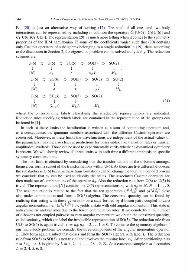
Eq. (20) is just an alternative way of writing (17). The total of all one- and two-bodyinteractions can be represented by including in addition the operators C1[U(6)], C2[U(6)] andC1[U(6)]C1[U(5)]. The representation (20) is much more telling when it comes to the symmetryproperties of the IBM hamiltonian. If some of the coefficients vanish such that (20) containsonly Casimir operators of subalgebras belonging to a single reduction in (19), then, accordingto the discussion in Section 2, the eigenvalue problem can be solved analytically. The reductionschemes are:

U(6) ⊃ U(5) ⊃ SO(5) ⊃ SO(3) ⊃ SO(2)

↓ ↓ ↓ ↓ ↓

[N ] nd τ ν1L ML

,

U(6) ⊃ SO(6) ⊃ SO(5) ⊃ SO(3) ⊃ SO(2)

↓ ↓ ↓ ↓ ↓

[N ] σ τ ν1L ML

,

U(6) ⊃ SU(3) ⊃ SO(3) ⊃ SO(2)

↓ ↓ ↓ ↓

[N ] (λ, µ) KL L ML

(21)

where the corresponding labels classifying the irreducible representations are indicated.Reduction rules specifying which labels are contained in the representation of the groups canbe found in [1].

In each of these limits the hamiltonian is written as a sum of commuting operators and,as a consequence, the quantum numbers associated with the different Casimir operators areconserved. Moreover, in these limits the wavefunctions are independent of the actual values ofthe parameters, making also clearcut predictions for observables, like transition rates or transferamplitudes, available. Those can be used to experimentally verify whether a dynamical symmetryis present. We will shortly review all three limits with each time a different emphasis on specificsymmetry considerations.

The first limit is obtained by considering that the transformations of the d-bosons amongstthemselves form a subset of the transformations within U(6). As there are five different d-bosonsthe subalgebra is U(5) because these transformations cannot change the total number of d bosonswe conclude that nd can be used to classify the states. The associated Casimir operators arethen made out of combinations of the operator nd. Also the reduction rule from U(6) to U(5) istrivial. The representation [N ] contains the U(5) representations nd with nd = N , N − 1, . . . 0.The next reduction is related to the fact that the ten generators (dĎd)

(1)m and (dĎd)

(3)m close

also under commutation and form a SO(5) algebra. The conserved quantity can be found byrealising that acting with these generators on a state formed by d-boson pairs coupled to zeroangular momentum, i.e. ((dĎdĎ)(0))|o〉, yields a state with odd angular momentum. This state isantisymmetric and vanishes due to the boson commutation rules. If we denote by τ the numberof d-bosons not coupled pairwise to zero angular momentum we obtain the conserved quantity,called seniority, which can label the irreducible representation of SO(5). The reduction rule fromU(5) to SO(5) is again trivial: τ = nd, nd − 2, . . . 1 or 0. To come to the symmetry algebra ofour many-body problem we consider the three components of the angular momentum operatorL . They form again a subset that closes and form the SO(3) algebra with label L . The reductionrule from SO(5) to SO(3) is non trivial and involves the missing label ν1. After partitioning τ asτ = 3ν1 +λ, L is given by L = λ, λ+1, . . . , 2λ−2, 2λ. As a concrete example τ = 4 containsL = 2, 4, 5, 6, 8.


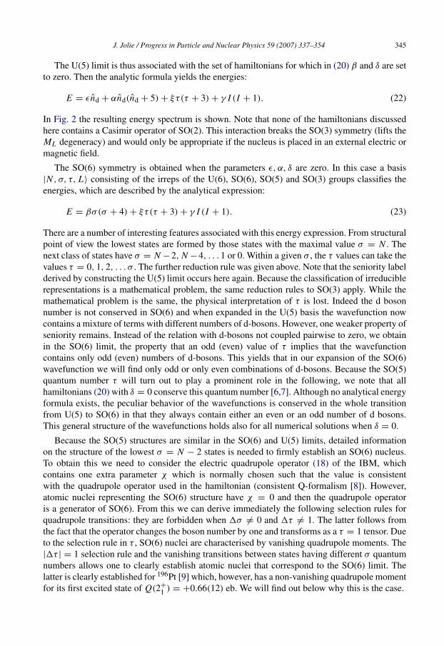
The U(5) limit is thus associated with the set of hamiltonians for which in (20) β and δ are setto zero. Then the analytic formula yields the energies:

E = εnd + αnd(nd + 5) + ξτ(τ + 3) + γ I (I + 1). (22)

In Fig. 2 the resulting energy spectrum is shown. Note that none of the hamiltonians discussedhere contains a Casimir operator of SO(2). This interaction breaks the SO(3) symmetry (lifts theML degeneracy) and would only be appropriate if the nucleus is placed in an external electric ormagnetic field.

The SO(6) symmetry is obtained when the parameters ε, α, δ are zero. In this case a basis|N , σ, τ, L〉 consisting of the irreps of the U(6), SO(6), SO(5) and SO(3) groups classifies theenergies, which are described by the analytical expression:

E = βσ(σ + 4) + ξτ(τ + 3) + γ I (I + 1). (23)

There are a number of interesting features associated with this energy expression. From structuralpoint of view the lowest states are formed by those states with the maximal value σ = N . Thenext class of states have σ = N −2, N −4, . . . 1 or 0. Within a given σ , the τ values can take thevalues τ = 0, 1, 2, . . . σ . The further reduction rule was given above. Note that the seniority labelderived by constructing the U(5) limit occurs here again. Because the classification of irreduciblerepresentations is a mathematical problem, the same reduction rules to SO(3) apply. While themathematical problem is the same, the physical interpretation of τ is lost. Indeed the d bosonnumber is not conserved in SO(6) and when expanded in the U(5) basis the wavefunction nowcontains a mixture of terms with different numbers of d-bosons. However, one weaker property ofseniority remains. Instead of the relation with d-bosons not coupled pairwise to zero, we obtainin the SO(6) limit, the property that an odd (even) value of τ implies that the wavefunctioncontains only odd (even) numbers of d-bosons. This yields that in our expansion of the SO(6)wavefunction we will find only odd or only even combinations of d-bosons. Because the SO(5)quantum number τ will turn out to play a prominent role in the following, we note that allhamiltonians (20) with δ = 0 conserve this quantum number [6,7]. Although no analytical energyformula exists, the peculiar behavior of the wavefunctions is conserved in the whole transitionfrom U(5) to SO(6) in that they always contain either an even or an odd number of d bosons.This general structure of the wavefunctions holds also for all numerical solutions when δ = 0.

Because the SO(5) structures are similar in the SO(6) and U(5) limits, detailed informationon the structure of the lowest σ = N − 2 states is needed to firmly establish an SO(6) nucleus.To obtain this we need to consider the electric quadrupole operator (18) of the IBM, whichcontains one extra parameter χ which is normally chosen such that the value is consistentwith the quadrupole operator used in the hamiltonian (consistent Q-formalism [8]). However,atomic nuclei representing the SO(6) structure have χ = 0 and then the quadrupole operatoris a generator of SO(6). From this we can derive immediately the following selection rules forquadrupole transitions: they are forbidden when 1σ 6= 0 and 1τ 6= 1. The latter follows fromthe fact that the operator changes the boson number by one and transforms as a τ = 1 tensor. Dueto the selection rule in τ , SO(6) nuclei are characterised by vanishing quadrupole moments. The|1τ | = 1 selection rule and the vanishing transitions between states having different σ quantumnumbers allows one to clearly establish atomic nuclei that correspond to the SO(6) limit. Thelatter is clearly established for 196Pt [9] which, however, has a non-vanishing quadrupole momentfor its first excited state of Q(2+

1 ) = +0.66(12) eb. We will find out below why this is the case.


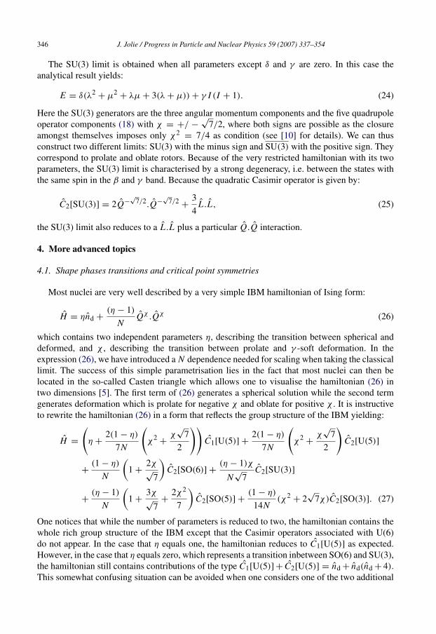
The SU(3) limit is obtained when all parameters except δ and γ are zero. In this case theanalytical result yields:

E = δ(λ2+ µ2

+ λµ + 3(λ + µ)) + γ I (I + 1). (24)

Here the SU(3) generators are the three angular momentum components and the five quadrupoleoperator components (18) with χ = +/ −

√7/2, where both signs are possible as the closure

amongst themselves imposes only χ2= 7/4 as condition (see [10] for details). We can thus

construct two different limits: SU(3) with the minus sign and SU(3) with the positive sign. Theycorrespond to prolate and oblate rotors. Because of the very restricted hamiltonian with its twoparameters, the SU(3) limit is characterised by a strong degeneracy, i.e. between the states withthe same spin in the β and γ band. Because the quadratic Casimir operator is given by:

C2[SU(3)] = 2Q−√

7/2.Q−√

7/2+

34

L.L, (25)

the SU(3) limit also reduces to a L.L plus a particular Q.Q interaction.

4. More advanced topics

4.1. Shape phases transitions and critical point symmetries

Most nuclei are very well described by a very simple IBM hamiltonian of Ising form:

H = ηnd +(η − 1)

NQχ .Qχ (26)

which contains two independent parameters η, describing the transition between spherical anddeformed, and χ , describing the transition between prolate and γ -soft deformation. In theexpression (26), we have introduced a N dependence needed for scaling when taking the classicallimit. The success of this simple parametrisation lies in the fact that most nuclei can then belocated in the so-called Casten triangle which allows one to visualise the hamiltonian (26) intwo dimensions [5]. The first term of (26) generates a spherical solution while the second termgenerates deformation which is prolate for negative χ and oblate for positive χ . It is instructiveto rewrite the hamiltonian (26) in a form that reflects the group structure of the IBM yielding:

H =

(η +

2(1 − η)

7N

(χ2

+χ

√7

2

))C1[U(5)] +

2(1 − η)

7N

(χ2

+χ

√7

2

)C2[U(5)]

+(1 − η)

N

(1 +

2χ√

7

)C2[SO(6)] +

(η − 1)χ

N√

7C2[SU(3)]

+(η − 1)

N

(1 +

3χ√

7+

2χ2

7

)C2[SO(5)] +

(1 − η)

14N(χ2

+ 2√

7χ)C2[SO(3)]. (27)

One notices that while the number of parameters is reduced to two, the hamiltonian contains thewhole rich group structure of the IBM except that the Casimir operators associated with U(6)do not appear. In the case that η equals one, the hamiltonian reduces to C1[U(5)] as expected.However, in the case that η equals zero, which represents a transition inbetween SO(6) and SU(3),the hamiltonian still contains contributions of the type C1[U(5)] + C2[U(5)] = nd + nd(nd + 4).This somewhat confusing situation can be avoided when one considers one of the two additional


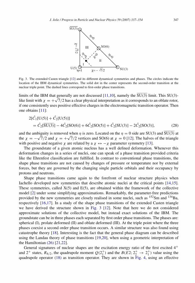
Fig. 3. The extended Casten triangle [12] and its different dynamical symmetries and phases. The circles indicate thelocation of the IBM dynamical symmetries. The solid dot in the center represents the second-order transition at thenuclear triple point. The dashed lines correspond to first-order phase transitions.

limits of the IBM that generally are not discussed [11,10], namely the SU(3) limit. This SU(3)-like limit with χ = +

√7/2 has a clear physical interpretation as it corresponds to an oblate rotor,

if one consistently uses positive effective charges in the electromagnetic transition operator. Thenone obtains [11]:

2[C1[U(5)] + C2[U(5)]]

= C2[SU(3)] − 4C2[SO(6)] + 6C2[SO(5)] + C2[SU(3)] − 2C2[SO(3)], (28)

and the ambiguity is removed when η is zero. Located on the η = 0 side are SU(3) and SU(3) atthe χ = −

√7/2 and χ = +

√7/2 vertices and SO(6) at χ = 0 [12]. The halves of the triangle

with positive and negative χ are related by a χ ↔ −χ parameter symmetry [13].The groundstate of a given atomic nucleus has a well defined deformation. Whenever this

deformation changes in a series of nuclei, one can speak of a phase transition provided criterialike the Ehrenfest classification are fulfilled. In contrast to conventional phase transitions, theshape phase transitions are not caused by changes of pressure or temperature nor by externalforces, but they are governed by the changing single particle orbitals and their occupancy byprotons and neutrons.

Shape phase transitions came again to the forefront of nuclear structure physics whenIachello developed new symmetries that describe atomic nuclei at the critical points [14,15].These symmetries, called X(5) and E(5), are obtained within the framework of the collectivemodel [2] under some simplifying approximations. Remarkably, the parameter-free predictionsprovided by the new symmetries are closely realised in some nuclei, such as 152Sm and 134Ba,respectively [16,17]. In a study of the shape phase transitions of the extended Casten trianglewe have derived the structure shown in Fig. 3 [12]. Note that here we do not consideredapproximate solutions of the collective model, but instead exact solutions of the IBM. Thegroundstate can be in three phases each separated by first order phase transitions. The phases are:spherical (I), prolate deformed (II) and oblate deformed (III). At the triple point where the threephases coexist a second order phase transition occurs. A similar structure was also found usingcatastrophe theory [18]. Interesting is the fact that the general phase diagram can be describedusing the Landau theory of phase transitions [19,20], when using a geometric interpretation ofthe Hamiltonian (26) [21,22].

General signatures of nuclear shapes are the excitation energy ratio of the first excited 4+

and 2+ states, R4/2, the quadrupole moment Q(2+

1 ) and the B(E2; 2+

2 → 2+

1 ) value using thequadrupole operator (18) as transition operator. They are shown in Fig. 4, using an effective


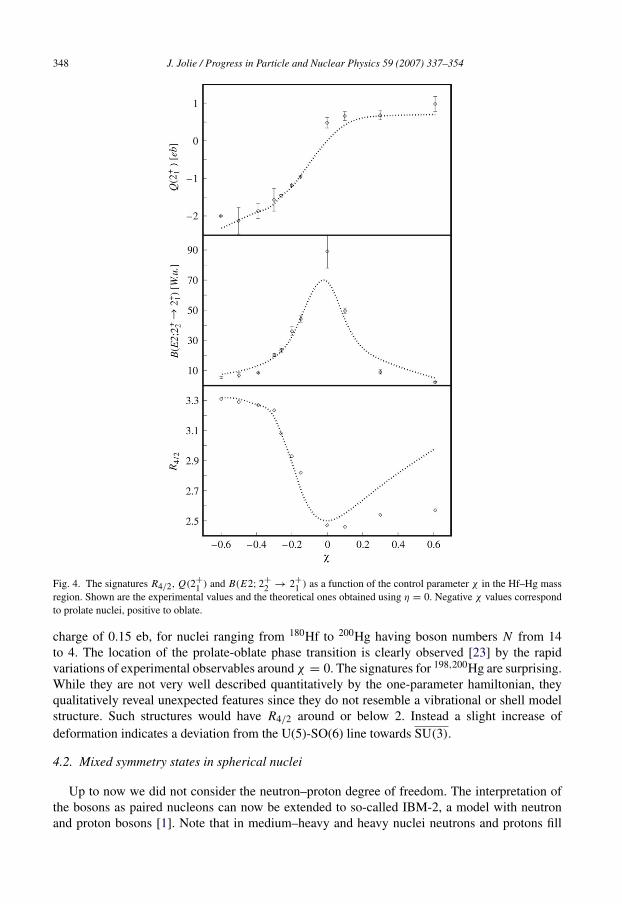
Fig. 4. The signatures R4/2, Q(2+

1 ) and B(E2; 2+

2 → 2+

1 ) as a function of the control parameter χ in the Hf–Hg massregion. Shown are the experimental values and the theoretical ones obtained using η = 0. Negative χ values correspondto prolate nuclei, positive to oblate.

charge of 0.15 eb, for nuclei ranging from 180Hf to 200Hg having boson numbers N from 14to 4. The location of the prolate-oblate phase transition is clearly observed [23] by the rapidvariations of experimental observables around χ = 0. The signatures for 198,200Hg are surprising.While they are not very well described quantitatively by the one-parameter hamiltonian, theyqualitatively reveal unexpected features since they do not resemble a vibrational or shell modelstructure. Such structures would have R4/2 around or below 2. Instead a slight increase ofdeformation indicates a deviation from the U(5)-SO(6) line towards SU(3).

4.2. Mixed symmetry states in spherical nuclei

Up to now we did not consider the neutron–proton degree of freedom. The interpretation ofthe bosons as paired nucleons can now be extended to so-called IBM-2, a model with neutronand proton bosons [1]. Note that in medium–heavy and heavy nuclei neutrons and protons fill


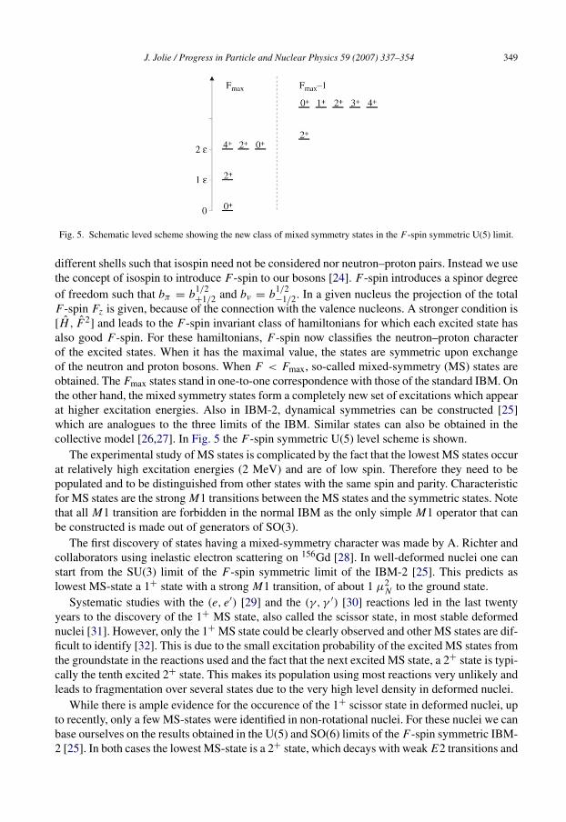
Fig. 5. Schematic leved scheme showing the new class of mixed symmetry states in the F-spin symmetric U(5) limit.

different shells such that isospin need not be considered nor neutron–proton pairs. Instead we usethe concept of isospin to introduce F-spin to our bosons [24]. F-spin introduces a spinor degreeof freedom such that bπ = b1/2

+1/2 and bν = b1/2−1/2. In a given nucleus the projection of the total

F-spin Fz is given, because of the connection with the valence nucleons. A stronger condition is[H , F2

] and leads to the F-spin invariant class of hamiltonians for which each excited state hasalso good F-spin. For these hamiltonians, F-spin now classifies the neutron–proton characterof the excited states. When it has the maximal value, the states are symmetric upon exchangeof the neutron and proton bosons. When F < Fmax, so-called mixed-symmetry (MS) states areobtained. The Fmax states stand in one-to-one correspondence with those of the standard IBM. Onthe other hand, the mixed symmetry states form a completely new set of excitations which appearat higher excitation energies. Also in IBM-2, dynamical symmetries can be constructed [25]which are analogues to the three limits of the IBM. Similar states can also be obtained in thecollective model [26,27]. In Fig. 5 the F-spin symmetric U(5) level scheme is shown.

The experimental study of MS states is complicated by the fact that the lowest MS states occurat relatively high excitation energies (2 MeV) and are of low spin. Therefore they need to bepopulated and to be distinguished from other states with the same spin and parity. Characteristicfor MS states are the strong M1 transitions between the MS states and the symmetric states. Notethat all M1 transition are forbidden in the normal IBM as the only simple M1 operator that canbe constructed is made out of generators of SO(3).

The first discovery of states having a mixed-symmetry character was made by A. Richter andcollaborators using inelastic electron scattering on 156Gd [28]. In well-deformed nuclei one canstart from the SU(3) limit of the F-spin symmetric limit of the IBM-2 [25]. This predicts aslowest MS-state a 1+ state with a strong M1 transition, of about 1 µ2

N to the ground state.Systematic studies with the (e, e′) [29] and the (γ, γ ′) [30] reactions led in the last twenty

years to the discovery of the 1+ MS state, also called the scissor state, in most stable deformednuclei [31]. However, only the 1+ MS state could be clearly observed and other MS states are dif-ficult to identify [32]. This is due to the small excitation probability of the excited MS states fromthe groundstate in the reactions used and the fact that the next excited MS state, a 2+ state is typi-cally the tenth excited 2+ state. This makes its population using most reactions very unlikely andleads to fragmentation over several states due to the very high level density in deformed nuclei.

While there is ample evidence for the occurence of the 1+ scissor state in deformed nuclei, upto recently, only a few MS-states were identified in non-rotational nuclei. For these nuclei we canbase ourselves on the results obtained in the U(5) and SO(6) limits of the F-spin symmetric IBM-2 [25]. In both cases the lowest MS-state is a 2+ state, which decays with weak E2 transitions and


strong M1 transitions to the normal states. Therefore there is no strong experimental signaturefor the excitation of this state from the groundstate, like in the scissor case. The advantage fornearly spherical atomic nuclei lies in the relatively lower level densities in vibrational nucleimaking it so that the 2+ MS state is expected to be the third up to sixth 2+ state and higher MSstates are also easier to observe. A first pure 2+ MS-state was established in 54Cr [33], but nohigher lying states of MS character could be identified.

During the last five years extended MS structures in vibrational nuclei have been establishedin 94Mo by N. Pietralla, Ch. Fransen and their collaborators, making this atomic nucleus thebest established case to test the predictions for these excitations. In the first experiments a NRFexperiment on 94Mo, performed at the Dynamitron accelerator of the University of Stuttgart,was combined with a beta-decay experiment at the FN Tandem accelerator of the University ofCologne. In the NRF experiments only 1+, 1− and 2+ states are populated. For the beta decayexperiment the 94Mo(p,n)94Tc reaction at 13 MeV was used to produce the Jπ

= (2)+ low-spinisomer of 94Tc which has a half-life of 52 min [34]. This (p, n) reaction favours the populationof the low-spin isomer compared to the 7+ groundstate, as the transferred angular momentumis only 6h. The beta decay of the low-spin isomer populates then the low-spin states in 94Mo.Gamma rays after beta decay were measured out of the beam which allowed the accumulation ofhigh statistics on a low background so that weak decay branches could be observed.

The observation of the 2+ MS state at 2067 keV in the NRF reaction is possible by the weaklycollective E2 decay (about 10% of the B(E2) value to the first excited state) that one obtains inthe F-spin symmetric SO(6) limit. In contrast, the first 2+ MS state in deformed nuclei is part ofa rotational band built on the 1+ MS state and its decay to the ground state is three times weaker.The essential proof to establish the MS character of both states formed the collective 1+

1 → 0+

1(0.16 µ2

N ) and 2+

3 → 2+

1 (0.48 µ2N ) M1 decays. An additional proof of the MS character of

the 1+

1 state is the observation of a very weak 1+

1 → 2+

1 (0.007 µ2N ) M1 decay and a strong

1+

1 → 2+

2 (0.43 µ2N ) M1 decay. The first observation of two MS states and the measurement of

their absolute decay probabilities forms the first detailed test of predictions on excited MS states.An excellent agreement with the SO(6) predictions in the F-spin symmetric version of IBM-2was obtained.

In order to understand the importance of the very small B(M1; 1+

1 → 2+

1 ) value in viewof symmetry, we recall that both the U(5) and SO(6) limit have a SO(5) subgroup. As alreadydiscussed in Section 2, the SO(5) symmetry makes it so that the wavefunction only containseither odd or even numbers of d-bosons. In the case of U(5) a single odd or even value occurs,but in SO(6) different values occur, but they are always all odd or all even. The M1 operatorsshould have an angular momentum of one and can therefore in lowest order only be made from ad boson number conserving operator due to simple vector coupling rules. To make the lowest 1+

MS state, due to the SO(5) symmetry, one needs an even number of d-bosons, e.g one neutronand one proton boson in U(5). For the first excited 2+

1 state we have, however, a single d-bosonstate in U(5) and only odd d-boson numbers in SO(6). Therefore the B(M1; 1+

1 → 2+

1 ) vanishes,as long as SO(5) is a conserved symmetry. A completely similar reasoning explains the vanishingof the B(M1; 1+

1 → 2+

3 ) observed with an experimental upper limit of 0.05µ2N [34]. Finally, in

the U(5) limit the d-boson number is fixed such that much more stringent selection rules follow.Notably B(M1; 1+

1 → 0+

1 ) is forbidden. This is the main argument to compare 94Mo to theSO(6) limit, although the energies are closer to the U(5) limit.

In a second experiment, 91Zr(α, n) was used to populate now medium-spin states in an ascomplete way as possible [35]. The energy of the α particles was chosen to be 15 MeV leading


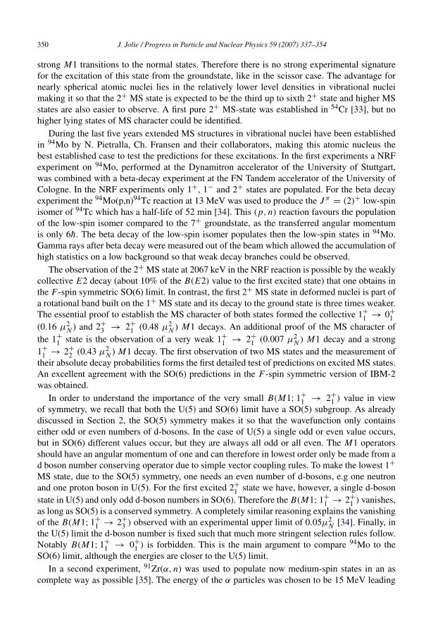
Fig. 6. Observed B(M1; 2+

i → 2+

2 ) values in 94Mo. For the 2+

3 and 2+

8 states no M1 transition was observed [36].

to an population of states with spins between J = 2 and J = 8 at a maximal excitation energyof 9 MeV. The experiment was performed at the FN Tandem accelerator of the University ofCologne using the Osiris spectrometer equipped with ten HPGe γ detectors. From the obtaineddata a state at 2965.4 keV could be identified as being the Jπ

= 3+ MS state. It was found thatthe 3+ MS state decays with pure M1 transitions to the symmetric 2+

2 and 4+

1 two phonon statesand with mixed E2/M1 transitions to the 2+

1 and MS 2+

3 states. The mixed symmetry characterof the 3+ state at 2965 keV could be established by the reduced B(M1) matrix elements ofabout one nuclear magneton to the 2+

2 and 4+

1 states and the collective E2 transition of tens ofWeisskopf units to the 2+

3 MS state.Using the same dataset also the second 2+ MS state could be identified as being the state

at 2870 keV [36]. In contrast to the 1+ and 3+ excited MS states, which both form the secondexcited state with the given spin value, at an energy of 3 MeV the excited 2+ MS state formsalready the sixth 2+ state. Therefore one needs a clear signature for its identification. Thissignature was the collective B(M1; 2+

6 → 2+

2 ) value of 0.35(11) µ2N , which is clearly well

above the corresponding value for the other excited 2+ states as shown in Fig. 6. Moreover, theidentification was not contradicted by the observed B(E2; 2+

6 → 2+

3 ) transition of 16+88−15 W.u.,

although the experimental error did not allow a definite conclusion.The last experiment on 94Mo was performed at the 7-MV electrostatic accelerator of the

University of Kentucky using inelastic neutron scattering. The main advantage of inelasticneutron scattering is the absence of the Coulomb barrier. Therefore the neutrons interact withthe atomic nucleus without energy loss. Thus the maximal excitation energy is given by theincident neutron energy, which can be varied. This is a paramount advantage compared to fusionevaporation reactions in which the nucleus is excited in a loosely defined and large energy range.In contrast to the similar situation in inelastic photon scattering, inelastic neutron scattering doesnot only make dipole and quadrupole excitations, but populates all states with spins up to about6 h.

Fransen et al. used in their experiment on 94Mo neutron beams with energies between2.4 and 3.9 MeV [37]. The excitation functions were measured in steps of 100 keV and theangular distributions were measured at 2.4, 3.3 and 3.6 MeV. The measured excitation functioncontradicts the earlier association of the 2739.9 keV level with the 2+

5 state and forms a new 1+

1state. The elimination of the feeding problem in inelastic neutron scattering allowed measurementof the lifetimes with about 10% error. As an example the lifetime of the 3+

2 and the now 2+

5


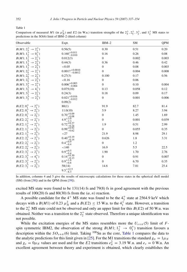
Table 1Comparison of measured M1 (in µ2

N ) and E2 (in W.u.) transition strengths of the 2+

3 , 2+

5 , 3+

2 , and 1+

2 MS states topredictions in the SO(6) limit of IBM–2 (third column)

Observable Expt. IBM–2 SM QPM

B(M1; 2+

3 → 2+

1 ) 0.56(5) 0.30 0.51 0.20B(M1; 1+

2 → 0+

1 ) 0.160+0.011−0.010 0.16 0.26 0.08

B(M1; 1+

2 → 2+

1 ) 0.012(3) 0 0.002 0.003B(M1; 1+

2 → 2+

2 ) 0.44(3) 0.36 0.46 0.42B(M1; 1+

2 → 2+

3 ) <0.05 0 0.08 0.003B(M1; 2+

5 → 2+

1 ) 0.0017+0.0010−0.0012 0 0.004 0.008

B(M1; 2+

5 → 2+

2 ) 0.27(3) 0.100 0.17 0.56B(M1; 2+

5 → 2+

3 ) <0.16 0 0.06B(M1; 3+

2 → 2+

1 ) 0.006+0.003−0.004 0 0.10 0.004

B(M1; 3+

2 → 4+

1 ) 0.075(10) 0.13 0.058 0.12B(M1; 3+

2 → 2+

2 ) 0.24(3) 0.18 0.09 0.17B(M1; 3+

2 → 2+

3 ) 0.021+0.016−0.012 0 0.001 0.006

0.09(2)B(E2; 0+

1 → 2+

1 ) 80(1) 91.9 82.7 81.4B(E2; 0+

1 → 2+

3 ) 11.0(10) 5.9 8.27 3.94B(E2; 0+

1 → 2+

5 ) 0.70+0.09−0.08 0 1.45 1.69

B(E2; 2+

3 → 2+

1 ) 4.9+3.0−2.3 0 0.001 0.039

B(E2; 1+

2 → 2+

1 ) 0.72+0.27−0.24 1.9 0.51 2.99

B(E2; 1+

2 → 2+

2 ) 0.99+0.92−0.62 0 0.055 0.35

B(E2; 1+

2 → 2+

3 ) <27 21.9 8.98 29.1B(E2; 2+

5 → 2+

1 ) 0.40+0.19−0.14 0.626 1.8 3.31

B(E2; 2+

5 → 2+

2 ) 0.4+0.9−0.4 0 1.2

B(E2; 2+

5 → 2+

3 ) <140 16.9 5.5 22.5B(E2; 3+

2 → 2+

1 ) 0.9+0.5−0.4 1.90 1.70 2.76

B(E2; 3+

2 → 4+

1 ) 0.14+0.30−0.13 0 0.91 0.007

B(E2; 3+

2 → 2+

2 ) 0.9+1.6−0.8 0 6.70 0.35

B(E2; 3+

2 → 2+

3 ) 58(14) 14.6 7.81 25.49.5+12.5

−8.3

In addition, columns 4 and 5 give the results of microscopic calculations for these states in the spherical shell model(SM) (from [38]) and in the QPM (from [39]).

excited MS state were found to be 131(14) fs and 79(8) fs in good agreement with the previousresults of 100(20) fs and 80(30) fs from the (α, n) reaction.

A possible candidate for the 4+ MS state was found to be the 4+

3 state at 2564.9 keV whichdecays with a B(M1) of 0.23 µ2

N and a B(E2) ≤ 15 W.u. to the 4+

1 state. However, a transitionto the 2+

3 MS state could not be observed and only an upper limit for this B(E2) of 50 W.u. wasobtained. Neither was a transition to the 2+

2 state observed. Therefore a unique identification wasnot possible.

While the excitation energies of the MS states resembles more the Uν+π (5) limit of F-spin symmetric IBM2, the observation of the strong B(M1; 1+

2 → 0+

1 ) transition favours adescription within the SOν+π (6) limit. Taking 100Sn as the core, Table 1 compares the data tothe analytic predictions for this limit given in [25]. For the M1 transitions the standard gπ = 1µNand gν = 0µN values are used and for the E2 transitions e2

π = 3.19 W.u. and eν = 0 W.u. Anexcellent agreement between theory and experiment is obtained, which clearly establishes the


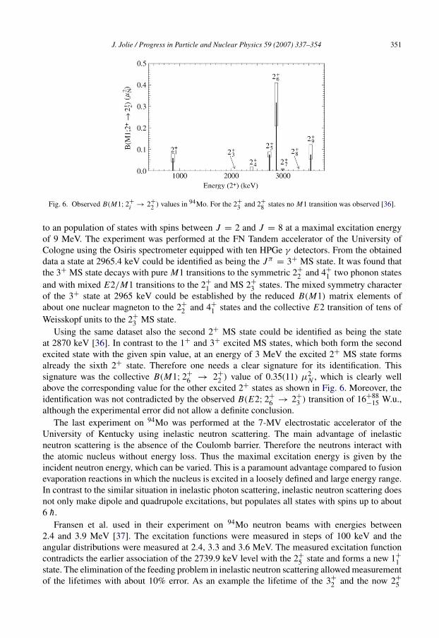
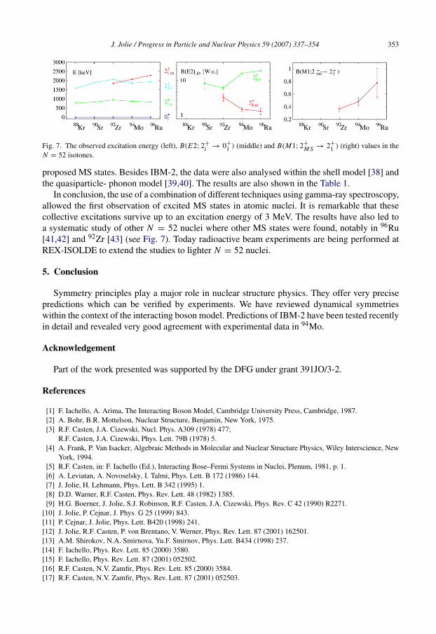
Fig. 7. The observed excitation energy (left), B(E2; 2+

i → 0+

1 ) (middle) and B(M1; 2+

M S → 2+

1 ) (right) values in theN = 52 isotones.

proposed MS states. Besides IBM-2, the data were also analysed within the shell model [38] andthe quasiparticle- phonon model [39,40]. The results are also shown in the Table 1.

In conclusion, the use of a combination of different techniques using gamma-ray spectroscopy,allowed the first observation of excited MS states in atomic nuclei. It is remarkable that thesecollective excitations survive up to an excitation energy of 3 MeV. The results have also led toa systematic study of other N = 52 nuclei where other MS states were found, notably in 96Ru[41,42] and 92Zr [43] (see Fig. 7). Today radioactive beam experiments are being performed atREX-ISOLDE to extend the studies to lighter N = 52 nuclei.

5. Conclusion

Symmetry principles play a major role in nuclear structure physics. They offer very precisepredictions which can be verified by experiments. We have reviewed dynamical symmetrieswithin the context of the interacting boson model. Predictions of IBM-2 have been tested recentlyin detail and revealed very good agreement with experimental data in 94Mo.

Acknowledgement

Part of the work presented was supported by the DFG under grant 391JO/3-2.

References

[1] F. Iachello, A. Arima, The Interacting Boson Model, Cambridge University Press, Cambridge, 1987.[2] A. Bohr, B.R. Mottelson, Nuclear Structure, Benjamin, New York, 1975.[3] R.F. Casten, J.A. Cizewski, Nucl. Phys. A309 (1978) 477;

R.F. Casten, J.A. Cizewski, Phys. Lett. 79B (1978) 5.[4] A. Frank, P. Van Isacker, Algebraic Methods in Molecular and Nuclear Structure Physics, Wiley Interscience, New

York, 1994.[5] R.F. Casten, in: F. Iachello (Ed.), Interacting Bose–Fermi Systems in Nuclei, Plenum, 1981, p. 1.[6] A. Leviatan, A. Novoselsky, I. Talmi, Phys. Lett. B 172 (1986) 144.[7] J. Jolie, H. Lehmann, Phys. Lett. B 342 (1995) 1.[8] D.D. Warner, R.F. Casten, Phys. Rev. Lett. 48 (1982) 1385.[9] H.G. Boerner, J. Jolie, S.J. Robinson, R.F. Casten, J.A. Cizewski, Phys. Rev. C 42 (1990) R2271.

[10] J. Jolie, P. Cejnar, J. Phys. G 25 (1999) 843.[11] P. Cejnar, J. Jolie, Phys. Lett. B420 (1998) 241.[12] J. Jolie, R.F. Casten, P. von Brentano, V. Werner, Phys. Rev. Lett. 87 (2001) 162501.[13] A.M. Shirokov, N.A. Smirnova, Yu.F. Smirnov, Phys. Lett. B434 (1998) 237.[14] F. Iachello, Phys. Rev. Lett. 85 (2000) 3580.[15] F. Iachello, Phys. Rev. Lett. 87 (2001) 052502.[16] R.F. Casten, N.V. Zamfir, Phys. Rev. Lett. 85 (2000) 3584.[17] R.F. Casten, N.V. Zamfir, Phys. Rev. Lett. 87 (2001) 052503.


[18] E. Lopez-Morelos, O. Castanos, Phys. Rev. C 54 (1996) 2374.[19] L. Landau, Phys. Z. Sowjet 11 (1937) 26; 11 (1937) 545. Reprinted in Collected Papers of L.D. Landau, Pergamon,

Oxford, 1965, p. 193.[20] L.D. Landau, E.M. Lifshitz, Statistical Physics, Part 1, in: Course of Theoretical Physics, vol. V, Butterworth-

Heinemann, Oxford, 2001.[21] J. Jolie, P. Cejnar, R.F. Casten, S. Heinze, A. Linnemann, V. Werner, Phys. Rev. Lett. 89 (2002) 182502.[22] P. Cejnar, S. Heinze, J. Jolie, Phys. Rev. C 68 (2003) 034326.[23] J. Jolie, A. Linnemann, Phys. Rev. C 68 (2003) 031301R.[24] T. Otsuka, A. Arima, F. Iachello, I. Talmi, Phys. Lett. B 76 (1978) 139.[25] P. Van Isacker, K.L.G. Heyde, J. Jolie, A. Sevrin, Ann. Phys. 171 (1986) 253.[26] A. Faessler, Nucl. Phys. 85 (1966) 653.[27] N. Lo Iudice, F. Palumbo, Phys. Rev. Lett. 41 (1978) 1532.[28] D. Bohle, A. Richter, W. Steffen, A. Dieperink, N. Lo Iudice, F. Palumbo, O. Scholten, Phys. Lett. 137B (1984) 27.[29] A. Richter, Prog. Part. Nucl. Phys. 34 (1995) 261.[30] U. Kneissl, H.H. Pitz, A. Zilges, Prog. Part. Nucl. Phys. 37 (1996) 349.[31] K. Heyde, A. Richter, Rev. Modern Phys. (in press).[32] D. Bohle, A. Richter, K. Heyde, P. Van Isacker, J. Moreau, A. Sevrin, Phys. Rev. Lett. 55 (1985) 1661.[33] K.P. Lieb, H.G. Boerner, M.S. Dewey, J. Jolie, S.J. Robinson, S. Ulbig, Ch. Winter, Phys. Lett. 215B (1988) 50.[34] N. Pietralla, C. Fransen, D. Belic, P. von Brentano, C. Friessner, U. Kneissl, A. Linnemann, A. Nord, H.H. Pitz,

T. Otsuka, I. Schneider, V. Werner, I. Wiedenhofer, Phys. Rev. Lett. 83 (1999) 1303.[35] N. Pietralla, C. Fransen, P. von Brentano, A. Dewald, A. Fitzler, C. Friessner, J. Gableske, Phys. Rev. Lett. 84

(2000) 3775.[36] C. Fransen, N. Pietralla, P. von Brentano, A. Dewald, J. Gableske, A. Gade, A. Lisetskiy, V. Werner, Phys. Lett. B

508 (2001) 219.[37] C. Fransen, N. Pietralla, Z. Ammar, D. Bandyopadhyay, N. Boukharouba, P. von Brentano, A. Dewald, J. Gableske,

A. Gade, J. Jolie, U. Kneissl, S.R. Lesher, A.F. Lisetskij, M.T. McEllistrem, M. Merrick, H.H. Pitz, N. Warr,V. Werner, S.W. Yates, Phys. Rev. C 67 (2003) 024307.

[38] A. Lisetskiy, N. Pietralla, C. Fransen, R.V. Jolos, P. von Brentano, Nucl. Phys. A677 (2000) 100.[39] N. Lo Iudice, Ch. Stoyanov, Phys. Rev. C 62 (2000) 047302.[40] N. Lo Iudice, Ch. Stoyanov, Phys. Rev. C 65 (2002) 064304.[41] H. Klein, A.F. Lisetskiy, N. Pietralla, C. Fransen, A. Gade, P. von Brentano, Phys. Rev. C 65 (2002) 044315.[42] N. Pietralla, C.J. Barton III, R. Krucken, C.W. Beausang, M.A. Caprio, R.F. Casten, J.R. Cooper, A.A. Hecht,

H. Newman, J.R. Novak, N.V. Zamfir, Phys. Rev. C 64 (2001) 031301.[43] V. Werner, et al., Phys. Lett. 550B (2002) 140.

Documents

Symmetry principles and nuclear structure