Synchronization and Coherence of Dynamical Systems:

Networks of Coupled Rossler Attractors

Kyle J. PounderDepartment of Mathematics

Saint Mary’s College of CaliforniaMoraga, California

Advisor: Dr. Timothy D. SauerDepartment of Mathematics

George Mason UniversityFairfax, Virginia

Abstract

In order to quantify the onset of phase and full synchronization in networks ofheterogeneous oscillators, we propose two order parameters. We then use these orderparameters to explore the onset of synchronization in various networks of noniden-tical Rossler attractors. We present our main findings, including: monotonic andnon-monotonic phase and full synchronization, as results of anti-synchronization and“network frustration”; (partial) phase synchronization in subgroups of networks; andgradual full synchronization in subgroups of networks and overall.

This final report is submitted in partial fulfillment of theNational Science Foundation REU and Department of Defense ASSURE Program.

George Mason UniversityJune 1, 2009–July 31, 2009

1 Introduction and Background

In the late twentieth century, while studying weather models, mathematician

Ed Lorenz was surprised to see that: when he changed his model’s inputs

only slightly, the model gave him not slightly, but drastically, different results.

Lorenz had, in fact, encountered a chaotic system.

In the study of dynamical systems, e.g. maps and differential equations, chaos refers to

one of three general types of behavior; the other two are fixed points and periodic orbits.

From these categories, we can identify one of the many interesting characteristics of chaos:

trajectories never repeat themselves. Another characteristic, as Lorenz discovered, is that

chaotic systems are extremely sensitive to initial conditions. Intrigued by these charac-

teristics and more, mathematicians have researched chaos in an attempt to understand it

further.

In addition to in weather models, chaos manifests itself in many other places in na-

ture, including: electrical circuits, lasers, and solar satellites [1]. There also exist several

primarily mathematical systems, e.g. the logistic map, that exhibit such behavior.

1.1 The Rossler attractor

The Rossler attractor is one well-known example of chaos. Designed in 1976 by Otto

Rossler, it was originally intended to “model equilibrium in chemical reactions” [2]. In

most contexts, though, it is more of a specimen for chaos studies.

The Rossler attractor is defined by the following three dimensional set of nonlinear,

ordinary differential equations

x = −ωy − z (1)

y = ωx+ ay (2)

1

z = f + z(x− c) (3)

where ω, a, f , and c are constant parameters. It is important to note that only for certain

ranges of these parameters is the behavior chaotic. In this paper, we will consider only

small variations of one set of parameters

a = 0.165 f = 0.2 c = 10 ω = 0.97

which are known to provide chaotic trajectories.

1.2 Synchronization and Coherence

In the study of chaos, one interesting phenomenon called synchronization [3, 4, 5] crops

up when two or more chaotic systems are coupled (i.e. they interact with each other). It

refers to when systems are coupled in such a way that they act “in unison” with each other

(while the chaotic behavior of the individual systems may remain).

There are many types of synchronization, but in this paper we will limit our discussion

to: coherence, phase synchronization and full synchronization.

Phase synchronization refers to when all trajectories are locked in phase (for an ex-

tended period of time). For example, we see in Figure (1) that the blue and green

trajectories are in phase but differ in amplitude.

Full synchronization refers to when all trajectories are locked in phase and amplitude

(for an extended period of time). In Figure (2), we see the two trajectories lie directly

on top of each other; that is, they agree in both phase and amplitude.

Coherence refers to any type of partial synchronization, e.g. phase synchronization of a

subset of oscillators, when the entire network is not synchronized in phase.

2

130 140 150 160 170 180 190 200

−15

−10

−5

0

5

10

15

time

X

Figure 1: Phase synchronization with two Rosslers

0 2 4 6 8 10 12 14 16 18 20−6

−4

−2

0

2

4

6

time

Y

Figure 2: Full synchronization with two Rosslers

3

We should point out that synchronization is not just a mathematical phenomenon.

In neurobiological networks, for example, where “irregular (chaotic) dynamics occur natu-

rally” [6], an understanding of synchronization would be a tremendous breakthrough. Also,

in engineering applications that involve chaotic systems, e.g. lasers, it would be useful to

understand the mechanisms that lead to the onset of coherence.

1.3 Motivation and Research Questions

Given the widespread appearance of chaos, and the potential implications of understanding

synchronization, many have sought to determine how it is that synchronization happens.

Restrepo et al [7] determined that there is a critical coupling strength that leads to the

onset of coherence. This critical coupling strength, they showed, depends on the uncoupled

dynamics of the oscillators and the adjacency matrix. This analysis, though, is limited by

their assumption that each oscillator has a large number of neighbors.

Ott et al [8] also explored synchronization in the case of globally coupled chaotic and

periodic oscillators.

The onset of synchronization in small, rather sparse networks remains minimally un-

derstood. In this paper we will investigate the onset of phase and full synchronization, as

well as partial synchronization (coherence), in sparse networks of heterogeneous Rossler

attractors. We are interested, in particular, in exploring the following questions:

1. Qualitatively speaking, how is the transition to phase and full synchronization? Is

it abrupt? Does synchronization seem to happen at once? Or is it gradual? Do

oscillators synchronize first in subgroups, then in larger groups, and then finally over

the entire network?

2. Is the onset of phase and full synchronization monotonic? That is, does a greater

coupling strength lead to more synchronization?

4

2 Research Methods

2.1 N Coupled, Nonidentical Rossler Attractors

In this paper, we will couple N nonidentical Rossler attractors. Let the ith oscillator be

defined by

xi =

xi

yi

zi

= F(xi) + kK

N∑j=1

Aij(xj − xi) (4)

where: F(xi) is the set of ordinary differential equations that define a single Rossler at-

tractor (Eqs. (1), (2), and (3)); A is the (N × N) adjacency matrix (i.e. Aij = 1 if the

jth Rossler drives the ith Rossler, Aij = 0 otherwise); k is the (positive) scalar coupling

strength; and K is the (3 × 3) diagonal coupling matrix (e.g. if K is the identity matrix,

then all three components of the Rosslers are coupled).

2.2 Order Parameters

We have seen that in the case of two coupled Rosslers, synchronization is relatively easy to

identify; in each component, we need only look at two curves and determine if they agree in

phase and possibly also in amplitude. However, when we scale up just even to ten Rosslers,

for example, the task of identifying synchronization (and particularly its onset) is much

more difficult. To identify phase synchronization, one must determine if all components

of the ten trajectories are locked in phase; and the more challenging part is to say when

this first happens. For full synchronization, it is a bit easier as one must only look to

see if all trajectories are identical. We shall note, though, that there are other interesting

possibilities—namely, partial synchronization—that are of interest, yet difficult to identify

5

with the eye. Clearly, inspection is not a good enough method for identifying all of these

interesting phenomena.

We propose, instead, two different “order parameters” that quantify the onset of syn-

chronization in its different forms: phase synchronization, full synchronization, and partial

forms of synchronization in between. In each case, the idea is to define a function, o(t),

that takes certain values for synchronization (i.e. either full or phase) and others for asyn-

chronization; in between, the values indicate some type of partial synchronization. Since

it is a function of time, we will look at the root mean square average, i.e. orms, over a

window of time, i.e. τ ≤ t ≤ τ + T , where the oscillator has relaxed onto the attractor.

O = orms =

√√√√√∫ τ+T

τ[o(t)]2 dt

T

This scalar quantity O will therefore indicate the coherence (or incoherence) of the network.

2.3 Full order parameter, R

The case of full synchronization is defined to be when all N oscillators in the network are

identical for an extended period of time. That is,

xi(t)− xj(t) ≡ 0 for 1 ≤ i, j ≤ N, τ0 ≤ t ≤ τ1, τ0 � τ1

Thus, for all t in the window, the quantity

N∑i=1

N∑j=1

Aij ‖xj(t)− xi(t)‖

6

is (close to) zero in the case of full synchronization and large in the case of asynchronization.

We have thus defined a quantity that tells us when full synchronization occurs, so we will

now only scale this quantity by dividing by two factors

N∑i=1

N∑j=1

Aij (5)

x?rms (6)

where (5) is the sum over the adjacency matrix, counting the number of connections in the

network, and (6) is the root mean square average of the chaotic oscillations of a represen-

tative oscillator, that is,

x?rms =

√√√√√∫ τ+T

τ[x?(t)]2 + [y?(t)]2 + [z?(t)]2 dt

T.

By dividing by (5), the quantity does not depend on the size of the network (i.e. the

number of ones in the adjacency matrix), and by dividing by (6), it does not depend on

the magnitude/units of the oscillations (i.e. it is dimensionless).

Let us then define

r(t) :=

N∑i=1

N∑j=1

Aij ‖xj(t)− xi(t)‖

x?rms

N∑i=1

N∑j=1

Aij

. (7)

We will now only consider the root mean square average of r(t) over a window of time after

7

Figure 3: A sine curve, two points x(t) and x(t− δt)

the oscillators have relaxed onto the attractor.

R = rrms =

√√√√√∫ τ+T

τ[r(t)]2 dt

T(8)

We will call this scalar quantity R the full synchronization order parameter, where R ≈ 0

implies full synchronization and R ≈ 1 implies asynchronization.

2.4 Phase order parameter, P

The case of phase synchronization is defined to be when all N oscillators in the network

are locked in phase for an extended period of time. To quantify this behavior, we will

rely on the oscillatory behavior of the x-component of the Rossler system. (Note: The

y-component is also oscillatory, so the same analysis could be done with that component;

the z-component, however, is not oscillatory, so it would not make a good choice.)

For the sake of illustration, let us assume for the moment that the x-component of the

8

Figure 4: A phase diagram of sin(t) v.s. sin(t− δt)

Rossler is a sine curve:

x(t) = sin(t).

Consider two points, x(t) and x(t−δt), where δt is one-fourth of an oscillation (i.e. δt = π/2

in our case). [See Figure (3).] Moreover, let us consider the complex number,

x(t) + ix(t− δt).

We can generate a phase diagram by plotting that number in the complex plane as t

increases. [See Figure (4).] The angle in the complex plane as we move around the circle1

is now a phase angle for the oscillator.1The circle is a result of a constant amplitude for the sine curve; in our chaotic systems, this may become

more elliptical because of varying amplitudes, but the normalization step will make this a non-issue.

9

Figure 5: Multiple sine curves synchronized in phase

Let us extend our analysis now to multiple sine curves that are synchronized in phase

xj(t) = Aj sin(t), j = 1, 2, 3.

[See Figure (5).] Without loss of generality, we will look at t = π/2. We see that the

complex numbers represented by each of these curves at t = π/2 are:

A1 sin(t = π/2) + iA1 sin(t− δt = 0) = A1 + i0

A2 sin(t = π/2) + iA2 sin(t− δt = 0) = A2 + i0

A3 sin(t = π/2) + iA3 sin(t− δt = 0) = A3 + i0

All have the same angle in the complex plane (i.e. 0), but different magnitudes (i.e. Aj).

Then, by normalizing these complex numbers (i.e. placing them on the unit circle), all of

the curves at t = π/2 would be represented by the same complex number: 1 + i0, with

phase angle 0 and magnitude 1. Since these curves are synchronized, the same holds for

10

Figure 6: The red trajectories are not phase synchronized, so the norm of their average isapproximately 0.65. The green trajectories are phase synchronized, so the norm of theiraverage is approximately 0.99.

all t.

In general: if trajectories are synchronized in phase, then (when normalized) they

will move together on the unit circle (i.e. same phase angle); however, if they are not

synchronized, then (when normalized) they will move separately around the unit circle

(i.e. different phase angles). To measure phase synchronization, then, we can average

these complex numbers over all oscillators. This average, which is itself a complex number,

will have a magnitude close to 1 if the curves are synchronized in phase. Otherwise, if the

complex numbers are distributed over the entire unit circle, then this average will have a

much smaller magnitude.

Therefore let us define

p(t) =1N

∥∥∥∥∥∥N∑j=1

xj(t) + ixj(t− δt)‖xj(t) + ixj(t− δt)‖

∥∥∥∥∥∥ . (9)

11

[See Figure (6) for an example of how p(t) works.] As we did with r(t), we will consider the

root mean square average of p(t) over a window of time after the oscillators have relaxed

onto the attractor.

P = prms =

√√√√√∫ τ+T

τ[p(t)]2 dt

T(10)

We will call this scalar quantity P the phase synchronization order parameter, where P ≈ 1

implies phase synchronization and P ≈ 0 implies asynchronization.

3 Results and Discussion

In all of the following investigations, we will use:

• Random initial conditions: The initial conditions for all components of all Rossler

attractors will be randomly generated between 0.8 and 1.2. By randomly generating

them, instead of choosing them to be identical, we can avoid the problem of trajec-

tories initially appearing synchronized. Also, we know that these initial conditions

lie within the basins of attraction of the Rossler attractors for the chosen parameter

values.

• RMS for R: We will use x?rms = 10.7177, where this has been computed as described

in Section (2.3) using a = 0.165, f = 0.2, c = 10, and ω = 0.97.

The values of the other parameters will be discussed as needed.

12

0 0.2 0.4 0.6 0.8 10

0.2

0.4

0.6

0.8

1

1.2

1.4

1.6

Coupling strength (k)

Full synch parameter (R) and Phase synch parameter (P)

RP

Figure 7: Two Rosslers phase and fully synchronize monotonically

Figure 8: Two Rosslers

13

Figure 9: Ten Rosslers, adjacency matrix with two subgroups

Figure 10: Simulation information

Two Rosslers Ten Rosslers, SubgroupsA See Figure (8) See Figure (9)a all 0.165 all 0.165f all 0.2 all 0.2c (1) 9 (1) 11 (6) 9 and

[6 6.1 10.9 11

]ω (1) 0.9 (1) 1.1 (6) 0.95 and

[0.91 0.92 1.04 1.05

]K

0 0 00 1 00 0 0

0 0 00 1 00 0 0

14

0 0.1 0.2 0.3 0.4 0.5 0.6 0.7 0.8 0.9 10

0.1

0.2

0.3

0.4

0.5

0.6

0.7

0.8

0.9

1

k

Coupling strength (k) v.s. Phase order parameter (P)

PP6

P4

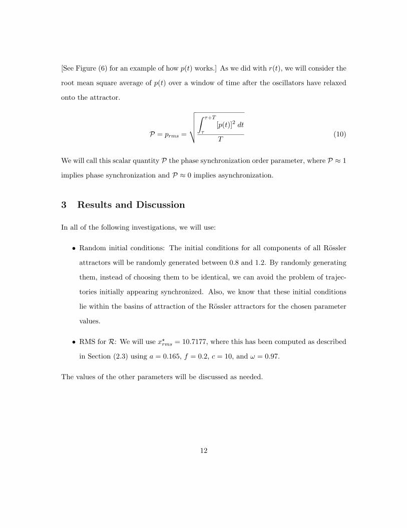
Figure 11: Phase synchronization, in both subgroups and overall

0 0.1 0.2 0.3 0.4 0.5 0.6 0.7 0.8 0.9 10

0.2

0.4

0.6

0.8

1

1.2

k

Coupling strength (k) v.s. Full order parameter (R)

RR6

R4

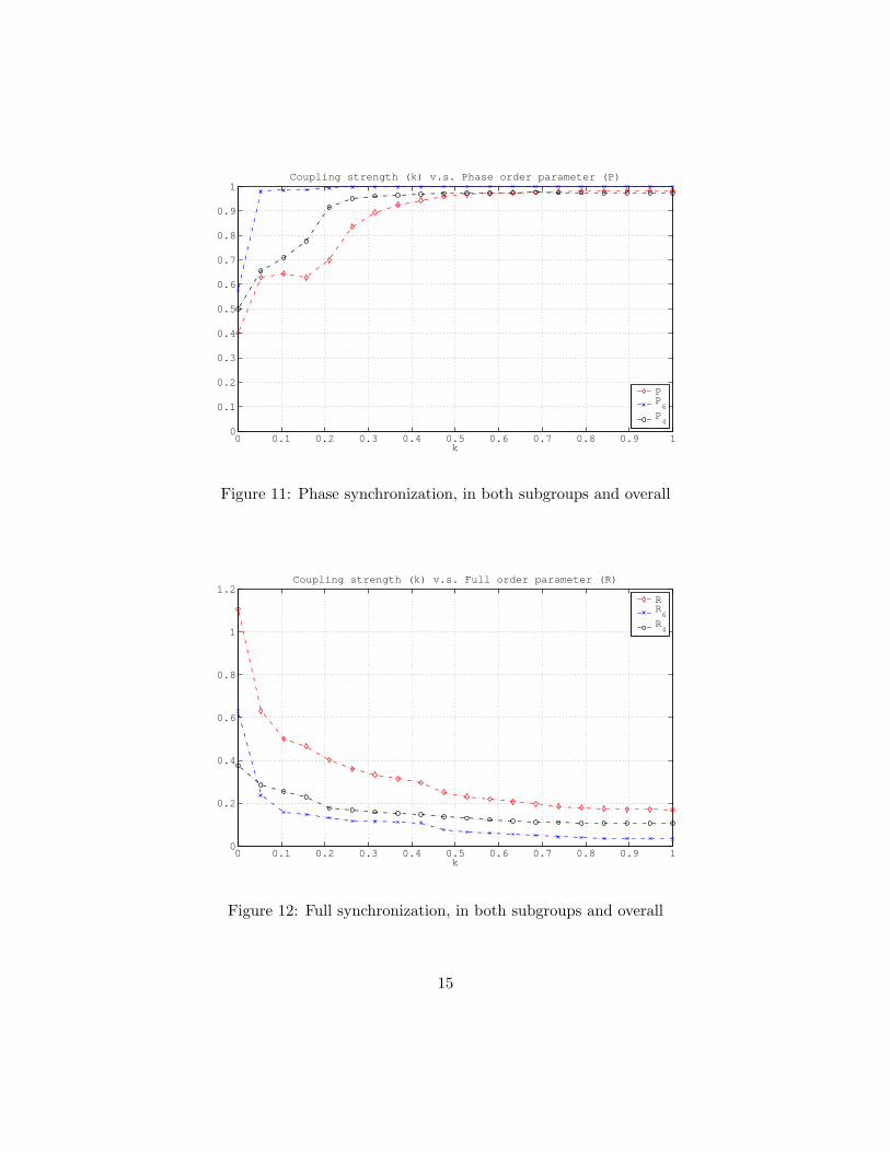
Figure 12: Full synchronization, in both subgroups and overall

15

3.1 Questions: Does phase synchronization happen all at once? Does

full synchronization happen all at once?

No. Neither phase synchronization nor full synchronization happens all at once. In fact,

both can happen gradually, or first in subgroups.

In the simple case of two coupled Rossler attractors [see Figure (10) for more informa-

tion], we find as in Figure (7) that neither phase synchronization nor full synchronization

happens all at once. In this case, both happen gradually as the coupling strength is in-

creased.

With the suspicion that synchronization is not instant in more complicated networks,

next we design a network of ten Rosslers that contains two subgroups: one of six identical

attractors, the other of four nonidentical attractors. There are two connections between

the networks. [See Figure (10) for more information.]

We find, as seen in Figure (11), that phase synchronization happens as one would expect

in a network with subgroups: first in the subgroups (and quicker in the subgroup of six

with more internal connections and more similar oscillators), then in the overall network.

One should also note that: (i) in the subgroup of six, P reaches 1 (unlike in the subgroup

of four and overall) because the oscillators in this subgroup are identical and can therefore

synchronize exactly in phase; and (ii) the overall network is eventually more synchronized

in phase than the subgroup of four, which can be understood by the similarity between

two oscillators in that group and the subgroup of six, therefore allowing eight oscillators to

synchronize (almost perfectly) in phase. This suggests that phase and full synchronization

is limited by the similarity between the oscillators.

As seen in Figure (12), we find that full synchronization happens gradually (both in the

subgroups and overall). It also seems that the rate of full synchronization is greatest in the

identical subgroup and in the overall network (with six identical oscillators, and two similar

16

Figure 13: Ten Rosslers, sparse adjacency matrix

to that group). This suggests that oscillator similarity affects the rate of synchronization.

3.2 Questions: Is phase synchronization monotonic? Is full synchroniza-

tion monotonic?

Not necessarily. We find for some networks that phase and full synchronization is mono-

tonic; for other networks, anti-synchronization and “network frustration” lead to non-

monotonic phase and full synchronization.

In the same case of two Rosslers that we investigated before, we see in Figure (7) that

both phase and full synchronization are monotonic. As the coupling strength, k, increases,

the phase order parameter P increases toward 1 and the full order parameter R decreases

toward 0. The monotonicity may be related to the simple interactions (i.e. only one

connection, two Rosslers) in this network. [See Figure (10) for more information on the

simulation.]

In the case of ten Rosslers, we find two behaviors which lead to non-monotonic syn-

17

Figure 14: Ten Rosslers, sparse adjacency matrix with two subgroups

Figure 15: Simulation information

10 Rosslers, Sparse 10 Rosslers, Sparse SubgroupsA See Figure (13) See Figure (14)a all 0.165 all 0.165f all 0.2 all 0.2c (5) 9 (5) 11 (6) 9 (4) 11ω (5) 0.95 (5) 1.05 (6) 0.95 (4) 1.05

K

0 0 00 1 00 0 0

0 0 00 1 00 0 0

18

0 0.05 0.1 0.15 0.2 0.250

0.2

0.4

0.6

0.8

1

1.2

Coupling strength (k)

Full synch parameter (R) and Phase synch parameter (P)

RP

Figure 16: Anti-synchronization leads to non-monotonic synchronization

1.176 1.1765 1.177 1.1775 1.178 1.1785 1.179 1.1795 1.18

x 104

−20

−15

−10

−5

0

5

10

15

20

time

x

Anti−synchronization

Figure 17: Anti-synchronization of one of the Rosslers (bold blue trajectory)

19

0 0.25 0.5 0.75 1 1.25 1.50

0.2

0.4

0.6

0.8

1

Coupling strength (k)

Full synch parameter (R) and Phase synch parameter (P)

RP

Figure 18: Network frustration leads to non-monotonic synchronization

7850 7860 7870 7880 7890 7900 7910 7920 7930−20

−15

−10

−5

0

5

10

15

20

time

x

Non−monotonic Synchronizationk = 0.3158

Figure 19: Trajectories with network frustration

20

7950 7960 7970 7980 7990 8000−20

−15

−10

−5

0

5

10

15

20

time

x

Non−monotonic Synchronizationk = 0.5526

Figure 20: Trajectories without network frustration

chronization in phase and overall: (partial) anti-synchronization and “network frustration.”

[See Figure (15) for more information on the simulations. Anti-synchronization occurs with

the sparse adjacency matrix; network frustration occurs with the sparse subgroup matrix.]

Anti-synchronization As seen in Figure (16), for coupling strengths, k, between 0.05

and 0.14, the phase order parameter P decreases. This happens because one of the

Rossler attractors anti-synchronizes with the rest of the network.2 [See Figure (17).]

It is surprising to see anti-synchronization with Rossler attractors coupled in this way.

We are unsure of the mechanism that leads to this phenomenon. R also increases

slightly between 0.05 and 0.06, but this increase is not attributable to any distinct

behavior or phenomenon.

Network frustration As seen in Figure (18), for coupling strengths, k, between 0.1 and2When computing P, anti-synchronization leads to points that are opposite each other on the unit circle;

then, when you add these points as complex numbers, the average has a smaller norm.

21

0.45, the phase order parameter P decreases; also, for k between 0.25 and 0.45, the

full order parameter R increases. This can be explained by the behavior seen for

k = 0.3158 in the interval 7850 ≤ t ≤ 7885 in Figure (19), which we are calling

network frustration. Although we are not sure of the exact mechanism causing this

behavior, it seems that the Rossler attractors (through interacting with each other)

are experiencing cycles of: being driven out of agreement in amplitude and in phase,

and then returning to coherence. At t = 7875, the Rosslers are essentially in one of

two phases; the oscillators in one group are at their maxima, while those in the other

group are at their minima. At this same time (t = 7875), there seem to be essentially

nine different amplitudes for the ten Rosslers. Then, by t = 7895, the Rosslers nearly

agree in phase and in amplitude. This pattern repeats itself again and again for this

coupling strength. When k increases to 0.5526, as seen in Figure (20), there is no

longer any network frustration; thus, P and R are higher and lower respectively. As

k continues increasing from this point, the network does not experience any more

frustration, and the order parameters continue monotonically.

4 Conclusions and Future Work

The proposed order parameters, R and P, successfully quantify the onset of partial, phase,

and full synchronization in networks of Rossler attractors. In general, the phase order

parameter could be used with any coupled attractors provided one of the components of

the attractors is oscillatory. The full order parameter could also be used in networks of

different attractors.

Using the order parameters, a few conclusions were drawn:

Synchronization not all at once. Neither phase nor full synchronization happens at

once. In our examples provided, phase synchronization happened both gradually

22

and in subgroups. Full synchronization happened gradually in all of our example

networks.

Monotonic and non-monotonic. Synchronization is not necessarily monotonic. Inter-

esting behaviors like anti-synchronization and network frustration can lead to non-

monotonic synchronization.

In future work, we would like to investigate:

More behaviors. We would like to continue exploring and observing the onset of syn-

chronization for different networks, including: adjacency matrices of varying sparsity,

the limit of nonidentical to identical oscillators, and more.

Analytic connections. We would like to explore analytic connections between network

topology, oscillator dynamics and the onset of synchronization in this case where

assumptions of many neighbors and globally coupled oscillators do not apply.

Applications. We would like to investigate potential applications of these order param-

eters. One particular application we have considered is in the detection of similar

(and dissimilar) oscillators using coupling and our order parameters.

5 Acknowledgements

This work was sponsored by the National Science Foundation REU and the Department

of Defense ASSURE programs.

23

References

[1] Wikipedia, Chaos theory, http://en.wikipedia.org/wiki/Chaos_theory.

[2] W. Zhang, S. Zhou, H. Li, and H. Zhu, Chaos, Solitons and Fractals 42, 1684 (2009).

[3] H. Fujisaka and T. Yamada, Prog. Theoretical Physics 69, 32 (1983).

[4] S. H. Strogatz, Sync: The emerging science of spontaneous order (Hyperion, New York,

NY, 2003).

[5] L. M. Pecora and T. L. Carroll, Phys. Rev. Letters 64, 821 (1990).

[6] Synchronization of chaos, http://inls.ucsd.edu/synch.html.

[7] J. G. Restrepo, E. Ott, and B. R. Hunt, Physica D: Nonlinear Phenomena 224, 114

(2006).

[8] E. Ott, P. So, E. Barreto, and T. Antonsen, Physica D: Nonlinear Phenomena 173, 29

(2002).

24