Synchrony and Desynchrony in Integrate-and-Fire …web.cse.ohio-state.edu/~wang.77/papers/CWJ99.pdf · Synchrony and Desynchrony in Integrate-and-Fire Oscillators 1597 tion 2.2. We

LETTER Communicated by David Terman

Synchrony and Desynchrony in Integrate-and-Fire Oscillators

Shannon R. CampbellDepartment of Physics, The Ohio State University, Columbus, Ohio 43210, U.S.A.

DeLiang L. WangDepartment of Computer and Information Science and Center for Cognitive Science,The Ohio State University, Columbus, Ohio 43210, U.S.A.

Ciriyam JayaprakashDepartment of Physics, The Ohio State University, Columbus, Ohio 43210, U.S.A.

Due to many experimental reports of synchronous neural activity in thebrain, there is much interest in understanding synchronization in net-works of neural oscillators and its potential for computing perceptual or-ganization. Contrary to Hopfield and Herz (1995), we find that networksof locally coupled integrate-and-fire oscillators can quickly synchronize.Furthermore, we examine the time needed to synchronize such networks.We observe that these networks synchronize at times proportional to thelogarithm of their size, and we give the parameters used to control therate of synchronization. Inspired by locally excitatory globally inhibitoryoscillator network (LEGION) dynamics with relaxation oscillators (Ter-man & Wang, 1995), we find that global inhibition can play a similar roleof desynchronization in a network of integrate-and-fire oscillators. Weillustrate that a LEGION architecture with integrate-and-fire oscillatorscan be similarly used to address image analysis.

1 Introduction

Different features of visual objects appear to be processed in different cor-tical areas (Zeki, 1993). How these features are linked to form perceptuallycoherent objects is known as the feature binding problem. Theoreticians haveproposed that correlations in the firing times of neurons may encode thebinding between these neurons (Milner, 1974; von der Malsburg, 1981). Aconsiderable amount of neurophysiological evidence supports this conjec-ture of temporal correlation (for a review see Singer & Gray, 1995; also seeLivingstone, 1996).

Based on the experimental findings, many oscillator networks have beenproposed in which synchronous oscillations link features together (syn-chrony implies the same frequency and phase). This particular form of tem-poral correlation was called oscillatory correlation (Wang & Terman, 1995). In

Neural Computation 11, 1595–1619 (1999) c© 1999 Massachusetts Institute of Technology

1596 S. R. Campbell, D. L. Wang, and C. Jayaprakash

oscillatory correlation two issues need to be addressed. The first is the needto achieve synchrony quickly in locally coupled networks. Our usage of theword quickly refers to a time of a few periods. This is based on biological data,which indicate that synchronous firings of neural groups begin two to threeperiods after the onset of stimulus (Singer & Gray, 1995). Locally couplednetworks are emphasized because a network with all-to-all coupling doesnot maintain pertinent geometrical and spatial information that is criticalfor perceptual processing (for further explanations see Sporns, Tononi, &Edelman, 1991; Wang, 1993). The second issue is how to desynchronize thephases of different objects rapidly and robustly so that segmentation occurs.

In this article we study integrate-and-fire oscillators, possibly the sim-plest model of neuronal dynamics. A single variable represents the mem-brane potential. When this variable attains a certain threshold, it is saidto fire, and it is reset to zero. When the oscillator fires, it sends excitationto its neighbors. Integrate-and-fire oscillators have frequently been studiedas models of neuronal behavior (Peskin, 1975; Mirollo & Strogatz, 1990).Several authors have noted the ability of locally coupled networks to syn-chronize (Mirollo & Strogatz, 1990; Corral, Perez, Diaz-Guilera, & Arenas,1995; Hopfield & Herz, 1995). However, it is not known how quickly thesenetworks synchronize. In computational terms, the time complexity of syn-chronization in these networks is unknown.

In one of the few studies systematically addressing locally coupled inte-grate-and-fire oscillators, Hopfield and Herz (1995) reported that a two-dimensional locally connected integrate-and-fire oscillator network (40 ×40) with excitatory couplings exhibits global synchrony (all oscillators firein unison) on long timescales (about 100 periods). Due to its convergencespeed, global synchrony was considered to be too slow to underlie biologicalinformation processing. When examining this phenomenon, we found thatsynchrony in the same size network can actually be achieved quickly (in twoto three periods) through appropriate adjustment of parameters. Furthernumerical investigations revealed a surprising scaling relation: the averagetime to synchrony increases as the logarithm of the system size in bothone-dimensional (1D) and two-dimensional (2D) systems.

Given that locally coupled integrate-and-fire oscillators synchronizequickly, we have already attained one of the aspects of oscillatory corre-lation: fast synchronization. The other aspect of oscillatory correlation isdesynchronization. In order to desynchronize different groups of oscillatorswhile maintaining synchrony within each group, we use the locally excita-tory globally inhibitory oscillator network (LEGION) architecture proposedby Terman and Wang (1995). This architecture relies on a single inhibitoryunit, which is coupled to every oscillator, to desynchronize different groupsof oscillators. To illustrate the potential of this network, we provide resultson some image segmentation tasks.

We define a system of integrate-and-fire oscillators in section 2.1. We thendescribe the behavior of two interacting integrate-and-fire oscillators in sec-

Synchrony and Desynchrony in Integrate-and-Fire Oscillators 1597

tion 2.2. We display our data indicating that the time to synchrony scalesas the logarithm of the system size for 1D and 2D systems in section 3; wealso describe how the system parameters are related to the rate of synchro-nization in this section. In section 4 we describe how we create a LEGIONnetwork with integrate-and-fire oscillators that can desynchronize multiplegroups of oscillators while maintaining synchrony within each group us-ing binary images. In section 5 we modify and extend this network so thatgray-level images can be processed. We demonstrate the potential of thisnetwork by segmenting real images. Section 6 provides further discussions.

2 Model Description and Behavior

2.1 Model Definition. A network of integrate-and-fire oscillators is de-fined as

xi = −xi + I0 +∑

j∈N(i)

JijPj(t), i = 1, . . . ,n, (2.1)

where the sum is over the oscillators in a neighborhood, N(i), about oscil-lator i. xi represents some voltage-like variable that we call the potential ofoscillator i. The parameter I0 controls the period of an uncoupled oscilla-tor. The threshold of an oscillator is set to 1. When xi = 1 the oscillator issaid to fire; its potential is instantly reset to 0, and it sends excitation to itsneighbors.

The interaction between oscillators, Pj(t), is defined as

Pj(t) =∑

mδ(t− tm

j ), (2.2)

where tmj represents the m firing times of oscillator j and δ(t) is the Dirac

delta function. When oscillator j fires at time t, oscillator i receives an in-stantaneous pulse. This pulse increases xi by Jij. If xi is increased above thethreshold, it will fire. Note that information is transmitted between oscilla-tors instantaneously, and thus the propagation speed is infinite.

The coupling is between nearest neighbors; that is, an oscillator interactswith two neighbors in 1D and four neighbors in 2D. The connection strengthfrom oscillator j to oscillator i is normalized as

Jij = α

Zi, (2.3)

where Zi is the number of nearest neighbors that oscillator i has, for exam-ple, Zi = 2 for an oscillator i at the corner of a 2D system. The constant αis the coupling strength. The normalization ensures that all oscillators re-ceive the same amount of stimulus and therefore have the same trajectory in


phase space when synchronous (Wang, 1995). As Wang (1993, 1995) pointedout, such weight normalization is critical for synchronization in less homo-geneous situations, such as open boundary conditions; it has been usedin later studies (Hopfield & Herz, 1995; Traub, Whittington, Stanford, &Jefferys, 1996). Note that there are only two parameters in system 2.1: thecoupling strengthα and I0. When oscillator i reaches its threshold, it will fire,and its value will be reset to zero. Oscillator i then sends an instantaneousimpulse to neighboring oscillator j. If oscillator j is induced to fire, then itsvalue is reset in the following manner:

xj(t+) = xj(t−)+ Jji − 1. (2.4)

Since oscillator j fires, oscillator i immediately receives excitation and thusxi(t+) = Jij. Because of this, the period of the synchronous system is shorterthan the period of a single uncoupled oscillator. The synchronous period ofthe system is given by

log(

I0 − αI0 − 1

). (2.5)

Hopfield and Herz (1995) called this particular realization of a network ofintegrate-and-fire oscillators Model A.

2.2 A Pair of Integrate-and-Fire Oscillators. We now describe the be-havior of a pair of integrate-and-fire oscillators. This section contains a shortsummary of some of the results that Mirollo and Strogatz (1990) derived.The trajectory of a single uncoupled oscillator can be solved analytically—x(φ) = f (φ) = I0(1 − exp(−γφ)), where γ = log(I0/(I0 − 1)), the periodof the oscillator, and φ can be thought of as a phase, or a local time vari-able. Note that the function f (φ) increases monotonically ( f ′(φ) > 0) andis concave down ( f ′′(φ) < 0). Mirollo and Strogatz (1990) showed that anall-to-all connected system of integrate-and-fire oscillators with positivepulsatile coupling as well as f ′(φ) > 0 and f ′′(φ) < 0, synchronizes. Wedisplay the temporal evolution of a pair of integrate-and-fire oscillators inFigure 1. The oscillators initially have different potentials, but the interac-tion quickly adjusts their trajectories so that they eventually fire in unison.When two or more oscillators fire at the same time, we call them synchronous.The spikes shown in Figure 1 when an oscillator reaches the threshold arefor illustrative purposes only.

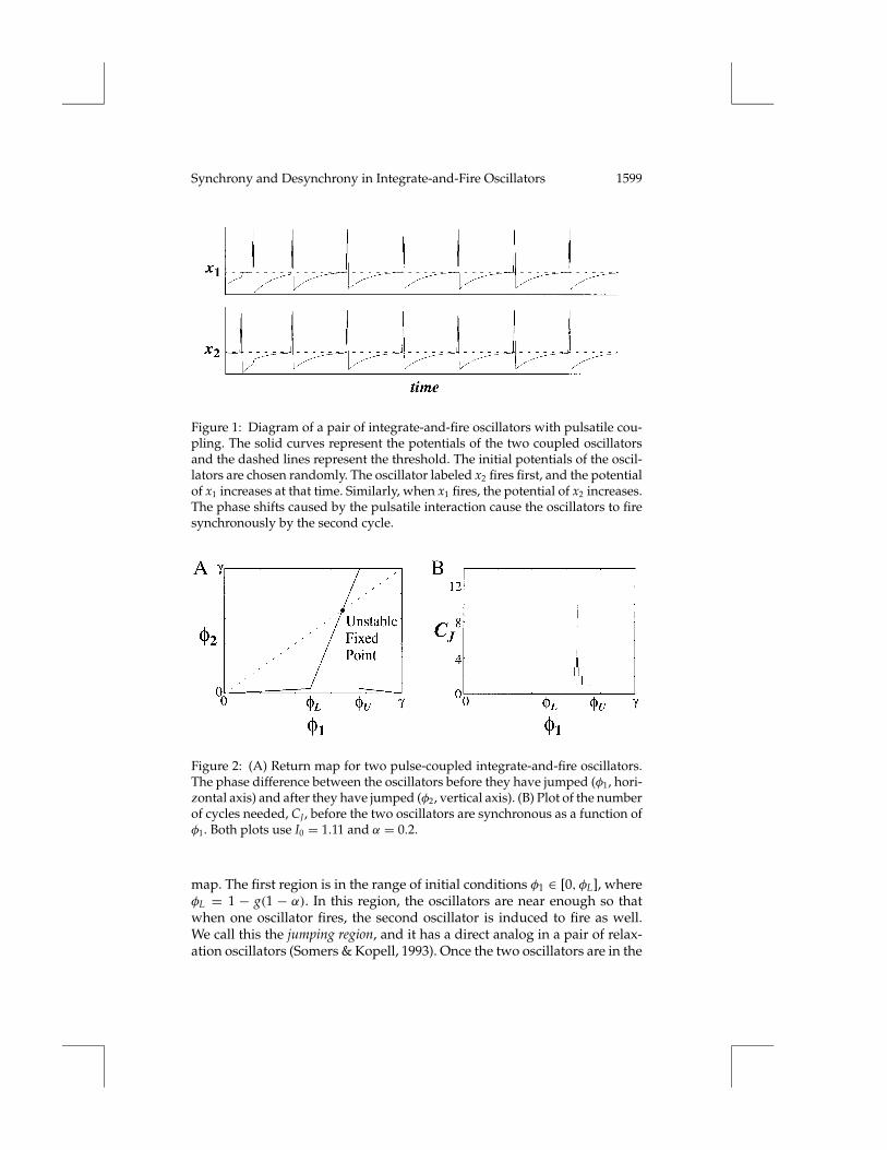
Using f (φ) and its inverse, g(x), one can calculate the return map (seeFigure 2A) for a pair of pulse coupled integrate-and-fire oscillators. A lineof slope 1 is also shown in Figure 2A for comparison. The horizontal axisrepresents the initial phase difference between the two oscillators, and thevertical axis represents the phase difference between the two oscillators af-ter they have both fired once. There are three different regions in the return


Figure 1: Diagram of a pair of integrate-and-fire oscillators with pulsatile cou-pling. The solid curves represent the potentials of the two coupled oscillatorsand the dashed lines represent the threshold. The initial potentials of the oscil-lators are chosen randomly. The oscillator labeled x2 fires first, and the potentialof x1 increases at that time. Similarly, when x1 fires, the potential of x2 increases.The phase shifts caused by the pulsatile interaction cause the oscillators to firesynchronously by the second cycle.

Figure 2: (A) Return map for two pulse-coupled integrate-and-fire oscillators.The phase difference between the oscillators before they have jumped (φ1, hori-zontal axis) and after they have jumped (φ2, vertical axis). (B) Plot of the numberof cycles needed, CJ, before the two oscillators are synchronous as a function ofφ1. Both plots use I0 = 1.11 and α = 0.2.

map. The first region is in the range of initial conditions φ1 ∈ [0, φL], whereφL = 1 − g(1 − α). In this region, the oscillators are near enough so thatwhen one oscillator fires, the second oscillator is induced to fire as well.We call this the jumping region, and it has a direct analog in a pair of relax-ation oscillators (Somers & Kopell, 1993). Once the two oscillators are in the


jumping region, they always fire at the same time, and it can be shown thattheir phase difference always decreases. The second region is in the rangeof initial conditions from [φL, φU], where φU = 1 − g( f (φL) − α). For theseinitial conditions, when the first oscillator fires, the other oscillator receivesexcitation, but is not induced to fire at the same time (as in the first firing ofx2 in Figure 1). Similarly, when the second oscillator fires, the relative phasebetween the two oscillators again changes, but the two oscillators do notfire in unison. In this region there is an unstable fixed point for which thephase between the oscillators does not change. In the third region, the firstoscillator fires and the second oscillator receives excitation but does not fireimmediately. When the second oscillator fires, the first oscillator receivesexcitation and is induced to fire a second time. We consider this third regionpart of the jumping region. In summary, this return map contains a rangeof initial conditions for which the two oscillators fire together and anotherset of initial conditions for which it may take several cycles before bothoscillators begin firing together.

In Figure 2B we display the number of cycles needed before the two os-cillators are in the jumping region. The horizontal axis in Figure 2B indicatesthe initial phase separation between the two integrate-and-fire oscillators,and the vertical axis indicates the number of cycles needed until the twooscillators are in the jumping region. As expected, initial conditions nearthe unstable fixed point require more cycles before synchrony occurs.

The derivative of the return map at the unstable fixed point is given by

(1+ α

I0

{α +

√α2 + 4I0(I0 − 1)2(I0 − 1)

})2

. (2.6)

This quantity gives one indication how repulsive the unstable fixed pointis; furthermore, the linearity of the second region in the return map of Fig-ure 2A is obtained for a wide range of I0, and hence the derivative at thefixed point. Therefore the derivative may indicate how fast the system ap-proaches the stable synchronous solution. The fixed point is unstable for allpositive values of α and all values of I0 > 1. For I0 À 1 the fixed point isstill unstable but the derivative is near 1, indicating a relatively slow ap-proach to synchrony. When I0 decreases the derivative increases, indicatinga faster approach to synchrony. We will compare equation 2.6 to the rate ofsynchronization in networks of oscillators in section 3.

The rate of synchronization, particularly phase compression betweenoscillators that have fired simultaneously, depends on the concavity of theoscillator trajectory in a more direct way. With f (φ) concave down, the os-cillators approach the threshold at a decreasing speed, and thus the timedifference between the two oscillators near the threshold can be quite largewhile the difference in their potentials is quite small. On the other hand,the time difference near the reset can be quite small while the potential


difference is quite large. When the two oscillators fire synchronously, theirpotential difference is kept constant right before and after the firing whiletheir time difference decreases. This results in a phase compression betweenthe oscillators, the amount of which is determined by the concavity. Thisanalysis is similar to an earlier analysis by Somers and Kopell (1993) on apair of relaxation oscillators, where the concavity of nullclines plays an anal-ogous role (see Terman & Wang, 1995, for a similar analysis for a networkof relaxation oscillators).

3 Synchrony in Integrate-and-Fire Oscillator Networks

We have observed that the average time to synchrony increases as the log-arithm of the system size in both 1D and 2D noiseless systems for randominitial conditions. Our observations are based on many trials of oscillatornetworks that were numerically integrated with an event-driven algorithm.For all data shown, we used the following procedure:

1. The potentials are chosen from the range [0,1].

2. Find the oscillator nearest to the threshold. The amount of time itneeds to fire is calculated and all the oscillators are advanced usingthis amount of time.

3. The oscillator at the threshold fires. The potential of this oscillatoris reset to zero, and the potentials of its neighboring oscillators areincreased using equation 2.3.

4. Check if any of the oscillators that have received excitation are abovethe threshold. If any oscillators are above the threshold, they are resetaccording to equation 2.4, and excitation is sent to their neighbors.Repeat this step until no oscillators are above the threshold.

5. Return to step 2.

All trials with locally coupled networks of integrate-and-fire oscillatorshave resulted in synchrony. Over 105 trials in which the initial conditionswere chosen randomly and uniformly in the range [0,1] have been recorded.These networks were also tested with other, more correlated initial con-ditions. Networks in which the initial conditions were spin waves alsoachieved synchrony. The speed with which networks with spin wave–typeinitial conditions attained synchrony was, on average, faster than that usingrandom initial conditions. For long-wavelength spin waves, the potentialsof the oscillators are near to each other, and one oscillator can cause many ofits neighbors to fire. Several large groups, or blocks, of oscillators form andfire synchronously during the first cycle. For short wavelengths that areinteger multiples of the lattice size, the oscillators also synchronize morequickly than with random initial conditions. Small blocks of synchronousoscillators form, and since these blocks are formed based on repeating


patterns of initial conditions, they also have a spatially repeating pattern.This process repeats until synchrony occurs. This implies that incommensu-rate wavelengths may take longer to synchronize because spatially repeat-ing patterns of blocks do not form and their interactions with one anotherwould not be uniform. This intuition does appear to be correct; incommen-surate wavelengths tend to have longer synchronization times. However, wecould not find any initial conditions whose resultant time to synchrony wasan order of magnitude larger than the average time to synchrony with ran-dom initial conditions (over 104 incommensurate frequencies were tested).Similar tests in 2D networks yield similar results. There are a few solu-tions that are not synchronous—for example, initial conditions in which thephase difference between neighboring pairs of oscillators is at the unstablefixed point shown in Figure 2A. In numerical tests with these initial condi-tions, floating-point errors eventually cause small perturbations away fromthis unstable solution, and synchrony quickly results. Furthermore, in trialswith periodic boundary conditions (a ring topology), solutions with trav-eling waves were never observed. Based on these extensive observations,we conclude that locally coupled networks of integrate-and-fire oscillatorsalways synchronize. Although all of our data have been gathered using oneor two specific integrate-and-fire oscillators, we claim that our results gen-eralize to the class of integrate-and-fire oscillators with positive coupling,f ′(φ) > 0, and f ′′(φ) < 0.

3.1 One-Dimensional Systems. We display the temporal evolution ofa 1-D network in Figure 3. The figure shows the firing times of all the os-cillators in a network of 400 oscillators. Time is shown along the verticalaxis, and the horizontal axis represents the index of the oscillators. Eachdot represents the firing time of one oscillator, and each line represents thefiring time of a block of oscillators. Near the bottom of the graph, there aremany single dots and small lines. These represent the fact that the oscillatorshave random initial conditions and initially have distinct firing times. Butquickly, by the time t = 5, blocks of various sizes have formed. Just aftertime t = 5, at the lower left of Figure 3, oscillators 1–20 fire simultaneously.This block formed from three smaller blocks. Near t = 30 there is a singlesolid line shown, indicating that all the oscillators fired at the same time.Underneath this line are two separate blocks of oscillators. One might atfirst wonder why these two large blocks have merged in just one cycle. Thisrepresents the fact that the system has an instantaneous propagation speed.When the oscillator at the left border of the right block receives excitation,it is induced to fire. When this oscillator fires, it sends excitation to its rightneighbor, which is also induced to fire, and this process repeats throughoutthe length of the right block. In the algorithm we use, the firing and resetof an oscillator are instantaneous, as are the excitatory pulses sent to neigh-boring oscillators. This results in an infinite propagation speed. Thus, nomatter how large a block is, it can merge with a neighboring block in one


Figure 3: Diagram displaying the evolution of a 1D network of 400 integrate-and-fire oscillators. The vertical axis represents time, and the horizontal axisrepresents the position of the oscillator in the chain. Each dot represents thefiring time of a single oscillator, and each line represents that of a block ofoscillators. The parameters are α = 0.2, I0 = 1.11.

cycle. The most striking feature of Figure 3 is that it is impossible to findan increase in the number of blocks. In fact, as shown in the appendix, thenumber of synchronized blocks never increases.

In Figure 4 we display data indicating that the time needed to synchro-nize a chain of size n oscillators increases in proportion to log10(n). Time isshown in units of periods. The averages are based on several hundred trialswith random initial conditions. The averages appear to lie on a straight linefor each of the three parameter pairs tested. Although only three data setsare displayed, our tests with other parameters yield a change only in theslope of the resulting line. The inset in this figure is shown to indicate thestandard deviation of the averages. The standard deviations for the otherdata sets are similar in that they remain nearly constant after the chain lengthbecomes larger than 20. We tested various combinations of α and I0 in theranges α ∈ [0.0025, 0.96] and I0 ∈ [1.01, 20]; all tested parameters resultedin a logarithmic relationship. In section 3.3 we discuss how these two pa-rameters relate to the slopes of the lines shown in Figure 4. We note thatonly several hundred trials were needed to compute the averages becauseour simulations indicated that the distribution of the synchronization timesdid not have a long tail (Campbell, 1997).


Figure 4: Average time needed for a chain of n oscillators to synchronize asa function of log10(n). Three symbols represent different parameters: squares:α = 0.48, I0 = 10; plus signs: α = 0.025, I0 = 1.1; diamonds: α = 0.2, I0 = 1.11.The data are based on approximately 300 trials with random initial conditions.The inset displays the diamond data along with the standard deviation of theaverages.

A heuristic understanding for our numerical results is as follows. As isdone typically in 1D problems in statistical mechanics, we focus on the do-main walls between adjacent clusters (blocks) of sites that are synchronized.As shown in the appendix, the number of domain walls, or equivalently thenumber of oscillator blocks, does not increase, so the only dynamically rel-evant process for a domain wall between two clusters is its disappearancewhen the two clusters become synchronized; the cluster that fires first sendsa pulse to its neighboring clusters, which then may also fire depending onthe difference in the dynamical variables of the two neighboring clusters.Since each domain wall has a nonzero probability of disappearing per unittime, one would expect that the walls disappear at a constant rate when av-eraged over the ensemble of initial conditions. Such a nonvanishing meanrate, r, for the removal of the domain walls automatically implies that thenumber of domain walls decreases as exp(−rt) and the entire system be-comes synchronized in a time proportional to the logarithm of the initial


Figure 5: Average times for an L × L network of oscillators to synchronize areplotted as a function of log10(2L−1). The solid diamonds are for the parametersα = 0.2, I0 = 2.0, and the open diamonds are for α = 0.2, I0 = 1.11. Each averageis computed from approximately 100 trials with random initial conditions. Theinset indicates the standard deviation for the solid diamond data.

number of domain walls. For the initial conditions we have considered, thenumber of domain walls is proportional to the size of the chain, and thisgives a heuristic explanation of our numerical results.

3.2 Two-Dimensional Systems of Oscillators. We display the averagesynchronization time for a 2D system as a function of log10(2L − 1) in Fig-ure 5, where the system size is L×L. Time is again shown in units of periods.In this 2D system, each oscillator is coupled to its four nearest neighbors,and the longest distance between any two oscillators (in terms of latticesites) is 2L− 1. The data indicate that the average time to synchrony scaleslogarithmically with the system size. We have tested more parameters thanshown in Figure 5, and all tested parameters yield an identical scaling rela-tion. The inset indicates the standard deviation for one set of data. Again,other sets of data show similar patterns of the standard deviation.

All trials with 2D networks resulted in synchrony. We tested various sizespin waves in the two directions and obtained similar results to those in


1D systems: synchrony was achieved regardless of the initial conditions.Traveling waves, rotating waves, or other desynchronous solutions werenever observed, even with periodic boundary conditions.

Unlike in 1D systems, we do not analytically know whether the numberof synchronized oscillator blocks does not increase in 2D. The situation in 2Dis considerably more complex; for example, it is possible that an oscillator isnot recruited to fire the first time it receives a pulse from one of its neighborsbut can after more of its neighbors have jumped. In our simulations, we havenot found a case where the number of blocks increases, which suggests thatour heuristic interpretation for 1D may carry over to 2D. We note that evenif the number of blocks increases occasionally, logarithmic scaling may stillhold because what matters for synchronization speeds is how groupingof oscillator blocks dominates breaking if the latter does occur. Note alsothat for 2D systems, blocks have more interaction paths and thus are moreconducive to synchronization.

We found that synchrony in the same size network as simulated in Hop-field and Herz (1995) can be achieved rapidly (in two to three periods) byusing different parameter values. We also tested integrate-and-fire oscilla-tor networks with the same parameter values used in Hopfield and Herz(1995). We confirmed their simulation results that a 40 × 40 network withI0 = 10 and α = 0.96 resulted in an average time to synchrony of approx-imately 100 periods. We also tested these parameters with different sizenetworks and found that, although it was very slow for a 40× 40 network,the average time to synchrony still held a logarithmic relation with the sys-tem size. In addition, we tested equivalent parameters in 1D systems andagain found the logarithmic scaling relation (see the squares in Figure 4).Thus, the reason that Hopfield and Herz (1995) did not observe rapid globalsynchrony is that the specific parameter values they used are not good forfast synchrony.

As we examine 2D systems, a natural question is how the rate of synchro-nization varies as the dimension of the system changes. We first define therate of synchronization as follows. The data indicate that 〈TS〉 ∼ 1

rSlog(n),

where 1rS

corresponds to the slope of a line from Figures 4 and 5. We refer torS as the rate of synchronization. In tests where the value ofα is held constantbut the dimension of the system changes from 1 to 2, we find that the rate ofsynchrony halves. When the individual coupling strengths between oscilla-tors are maintained—α doubles as the system dimension increases from 1 to2—we find that the rate of synchronization remains approximately the samebetween 1D and 2D systems. This indicates that the rate of synchronizationis controlled by the individual connection weights between oscillators andnot the total connection weights to each oscillator.

3.3 Rate of Synchronization. We now describe how the rate of synchro-nization is related to the system parameters. It is reasonable to expect that


the overall scale is set by the behavior of a pair of oscillators; the derivativeof the return map given by equation 2.6 describes the rate at which the twooscillators are repelled from the unstable fixed point after one iteration. Incontinuous time (measured in units of the period of an oscillator), the ratecan be approximated by an exponential (1 + rS)

2 ≈ exp(2rS) and thus rS,defined by

rS = αS

I0

αS +√α2

S + 4I0(I0 − 1)

2(I0 − 1)

, (3.1)

can be used to set the rate scale to measure synchrony. In equation 3.1, αSrepresents the single connection strength between a pair of oscillators inthe network, as opposed to the total connection strength, which is givenby α. In Figure 6 we show a scatter plot of actual rates of synchronizationcomputed from numerical simulations with respect to rS given by equa-tion 3.1. The figure shows good proportionality between the equation andthe measured rates of synchrony (the majority of points lie along a straightline). Note that the rates of synchrony for this figure range from 0 to 1,which implies that we tested a wide range of parameters. Rates of syn-chrony near 0 yield extremely slow synchronization rates, and a rate ofsynchrony near 1 means that 10 cycles are enough to synchronize a chainof 1010 oscillators.

Several data points in Figure 6 exhibit a significant deviation from thestraight line. The majority of these points that are not along the line resultfrom values of the coupling strength that are greater than 0.8. This is as ex-pected because as α nears 1, the period of the oscillator system approaches0; the oscillators fire frequently but change their relative phase only slowly.As α nears 1, the time to synchrony becomes infinite. At α = 1 systemequation 2.1 is meaningless because the oscillators are constantly firing andresetting. Our data reflect this understanding because as the coupling be-comes greater than 0.8, approximation 3.1 becomes worse. Our data alsoindicate that this approximation is not good for values of I0 < 1.05. Notethat our argument for using rS to set the rate scale is valid if the fixed pointis in the middle of the second region (see Figure 2A). As I0 becomes smallerthan 1.05, the derivative gets very large, and the second region becomesvery narrow, and so the phase difference gets into the jumping region (thefirst region or the third region) rapidly. Since the phase difference does notspend enough time in the vicinity of the fixed point, we think that the rateof deviation from the fixed point no longer sets the scale reliably. In thiscase, rapid synchronization is mainly accounted for by the behavior in thejumping region (the first and the third region).

3.4 Heterogeneity. We have studied the behavior of the system with het-erogeneity in the intrinsic frequencies. When the variations are bounded—


Figure 6: Scatter plot of the predicted rate of synchrony from equation 3.1against the measured value. The measured rates of synchrony were obtainedfrom oscillator chains by randomly choosing n (from 150 to 1000), the couplingstrength (from 0 to 1), and I0 (from 1 to 100), and calculating the average timeto synchrony using 100 trials with random initial conditions. The figure showsthe results with approximately 575 different parameter choices.

for example, within 5%—synchrony is still achieved in both 1D and 2Dsystems. When the distribution of frequencies is gaussian, the network canachieve synchrony only if the variance is small and the system size is mod-est (say, 100 in a 1D chain). The oscillators do not follow the same pathin phase space since their speeds depend on the frequency; nevertheless,with a sufficiently small difference in frequencies, when the fastest oscilla-tor jumps, it can induce the rest of the network to fire simultaneously. Forlong chains or larger variances of intrinsic frequencies, the chain evolves toclusters of synchronous oscillators. The border between clusters containsneighboring oscillators whose intrinsic frequence difference is too large forthem to fire together; this occurs due to the tails in the gaussian distri-bution. We have not studied the effects of heterogeneity systematically. Inparticular, the effect on the rate of synchronization has not been investi-gated.


4 Desynchrony

The locally coupled networks of integrate-and-fire oscillators have beenshown to have the property that synchrony is quickly achieved. But a systemthat only achieves synchrony is not very useful for information processing,since such a system is dissipative and almost all information is lost. In orderto perform computations, some other mechanisms must exist that can storeor represent information. In oscillatory correlation, the different phases ofoscillators encode binding and segregation information.

In order to create a network of integrate-and-fire oscillators for oscillatorycorrelation, we need a mechanism that desynchronizes different oscillatorgroups. Such a mechanism would need to be long range since the phases ofdifferent oscillator groups need to be desynchronous regardless of their po-sitions in the network. Our construction employs a global inhibitor, and thearchitecture of our network is identical to the LEGION networks proposedby Terman and Wang (1995). The main difference is that the basic unit in ournetwork is an integrate-and-fire oscillator rather than a relaxation oscillator.Figure 7A displays a diagram of the LEGION architecture.

We now define a LEGION network that uses integrate-and-fire oscillatorsas its basic units. The activity of each oscillator in the network is described by

xi = −xi + Ii +∑

j∈N(i)

JijPj(t)− G(t), (4.1)

where N(i) represents the four nearest neighbors of oscillator i. The param-eter, Ii, is now dependent on the input image; we refer to this parameteras the stimulus given to oscillator i. In this section we discuss binary im-ages. The respective stimulus for each oscillator is either Ii > 1 or Ii = 0. IfIi > 1 we call oscillator i stimulated. If an oscillator does not receive stim-ulus, Ii = 0, its potential decays exponentially toward zero. As before, thethreshold for each oscillator is 1. The interaction term, Pj(t), is the same as inequation 2.2. Only neighboring oscillators that both receive stimulus havea nonzero coupling strength. The connection strengths are normalized sothat all stimulated oscillators receive the same sum of connections and thushave the same frequency. However, we use a slightly modified version ofequation 2.3 to reflect that the input to oscillator i is now normalized bythe number of stimulated neighbors coupled with i. All of the above canbe neurally implemented by dynamic normalization of neural connections(Wang, 1995).

The global inhibitor, G(t), sends an instantaneous inhibitory pulse to theentire network when any oscillator in the network fires. It is defined as

G(t) = 0δ(t− tmj ), ∀j,m, (4.2)

where tmj represent the m firing times of the jth oscillator. The constant 0

is less than the smallest coupling strength between neighboring oscillators.


Figure 7: (A) Diagram of the network architecture. Each oscillator has localexcitatory connections. The global inhibitor is coupled with every oscillator inthe network. (B) Input image. The black squares represent those oscillators thatreceive stimulus, and the oscillators corresponding to the white squares receiveno stimulus. (C) Temporal activities of all units comprising each of the fourobjects in (B). The parameters are Ii = 1.05 for oscillators receiving stimulus,α = 0.2, and 0 = 0.01.


When an oscillator fires, the global inhibitor serves to lower the potential ofall oscillators, but because this impulse is not as large as the excitatory signalbetween neighboring oscillators, it does not destroy the synchronizing effectof the local couplings (see Terman & Wang, 1995). In this fashion, a connectedregion of oscillators receiving input synchronizes as the system evolves intime. This region of oscillators has no direct excitatory connections withother spatially separate regions of oscillators. It will, however, interact withother groups through the global inhibitor. This interaction inhibits otherblocks of oscillators from firing at the same time.

We now demonstrate the ability of this network to perform oscillatorycorrelation. In Figure 7B we display an input image with four objects and inFigure 7C the network response. The four graphs in Figure 7C display thecombined potentials of all the oscillators comprising each of the four ob-jects. The oscillators have random initial conditions varying uniformly from0 to 1. Initially many oscillators fire; the effect of the global inhibitor can beseen in the jitter, or lack of smoothness, in the potentials of the oscillatorsduring this time. As the system evolves, clusters of oscillators begin to form,and the curves become smoother because the global inhibitor does not sendinhibitory impulses as often. By the third cycle, each group of oscillatorscomprising a distinct object is almost perfectly synchronous, and the dif-ferent oscillator groups have distinct phases. Oscillators that do not receiveexcitation (not shown) experience an exponential decay toward zero andare periodically perturbed by the small inhibitory signals from the globalinhibitor.

In this network, there is an unlimited number of oscillator groups thatcan be segmented. In other words, the segmentation capacity is infinite.Imagine two groups of oscillators that have nearly the same phase. Whenthe first group fires, the potential of the second group of oscillators decreasesby 0. Thus, the second group needs to traverse the distance 0 before it canfire. This implies that there is a finite amount of time between the firingsof two consecutive groups. This also implies that as the number of groupsincreases, the period of the system increases. Simulations support the abovestatements, and we have segmented more than 100 groups of oscillators.

5 Image Segmentation

In the previous section, we segmented four black objects on a white back-ground in a 20×20 image. Since our study suggests that there is a logarithmicscaling relation between the time to synchrony and the network size, we ex-pect to be able to use this same network to perform image processing taskswith much larger images quickly.

In order to segment gray-level images, we alter how the connectionweights and values of Ii are chosen. The alterations are variations of themethods proposed in Wang and Terman (1997). Let the intensity of pixel ibe denoted by pi. If |pi−pj| is less than a given threshold, then the two pixels


are said to satisfy the pixel difference test. Two oscillators have a nonzerocoupling strength only if they are neighbors (we now use the eight nearestneighbors of i) and if their corresponding pixel values satisfy the pixel dif-ference test. The weights of the connection strengths are determined usingequation 2.3, except that Zi now represents the number of neighboring pix-els of i that pass the pixel difference test. The stimulus Ii for each oscillatoris chosen in the following manner. We examine a region Q(i) centered onpixel i. Q(i) is a neighborhood about oscillator i that contains more pixelsthan N(i). If half of the pixels in Q(i) satisfy the pixel difference test, thenpixel i is likely within a homogeneous region, and we set the stimulus, Ii, toa value IL, which is greater than 1. Such an oscillator is called a leader (Wang& Terman, 1997) and is able to oscillate by itself. If Q(i) contains no pixelsthat satisfy the pixel difference test, the corresponding oscillator receives nostimulus and does not oscillate. Otherwise oscillator i is given a stimulus IN,which is less than but near 1 and is said to be a near-threshold oscillator. Anear-threshold oscillator is able to fire only through interactions with otheroscillators. In this fashion, only regions of sufficient size and with smoothlyvarying intensities will contain leaders. These leaders will oscillate and caninduce neighboring oscillators that are near threshold to oscillate. Regionswith high-intensity variations will not exhibit oscillatory activity and arereferred to as the background.

The rules for the connection weights and oscillator stimuli describedabove have been implemented in an integrate-and-fire oscillator network,and we display the segmentation results for two real images in Figure 8.Figure 8A displays an aerial photograph. In Figure 8B we display the seg-mentation results of our network. Each group of synchronous oscillatorsis represented by a single gray-level intensity. Inactive oscillators compris-ing the background are colored black. There are 29 regions segmented, al-though it is not easy to discern every different gray level. We also segmenta computerized tomography (CT) image of a slice of a human head. Theoriginal gray-level image is shown in Figure 8C. The bright areas indicatebone structure. Our segmentation result is shown in Figure 8D and contains25 segments. The different bone structures are segmented, except for twoof the smaller bones that do not contain many pixels. Regions of soft tissueare also segmented.

Our demonstration here is not meant to be a claim that we producebetter segmentation results with these images. Rather, our objective is toillustrate the utility of integrate-and-fire oscillator networks for such tasks.The distinctive feature of such networks for image segmentation includes itsneurobiological basis and its parallel and distributed nature of computation.

6 Discussion

We have investigated the time complexity of synchronization, in particularthe scaling relation between the time to synchrony and the system size, in


Figure 8: (A) Aerial image with 128×128 pixels. (B) Segmentation results for (A).The network produced 29 different synchronized groups. Each synchronizedgroup is represented by a single gray level. Black pixels represent oscillators thatdo not oscillate. The threshold for the pixel difference test is 19, Qi is a region ofsize 7 × 7, with IL = 1.025, IN = 0.99, α = 0.2, and 0 = 0.01. (C) 128 × 128 CTimage of a slice of a human head. (D) Segmentation results for (C). The networkproduced 25 different groups of synchronized oscillators. The threshold for thepixel difference test is 15, Qi is a region of size 9× 9, and the other parametersare as listed above.

locally coupled networks of integrate-and-fire oscillators. Our data stronglysuggest that 1D and 2D systems of identical oscillators synchronize at timesproportional to the logarithm of the system size. We have also given anapproximation relating the rate of synchronization to the system param-eters. Remarkable rates of synchronization can be achieved. For example,one can choose parameters so that a chain of 106 oscillators can synchro-nize in approximately six cycles. This is opposite to the conclusion reachedby Hopfield and Herz (1995), who discount global synchrony in such net-works as too slow to be useful in biological computations, and instead use


networks capable of fast local synchrony to perform computations. In localsynchrony, small clusters of oscillators fire at the same time, and the entirenetwork may consist of many such clusters.

We also used integrate-and-fire oscillators to create an oscillator networkthat performs oscillatory correlation. We found that using the LEGION ar-chitecture (Terman & Wang, 1995), we were able to create a global inhibitorthat serves the purpose of desynchronizing different groups of oscillatorswhile maintaining synchrony within each group of oscillators. Our seg-mentation network is different in several ways from that proposed for im-age segmentation by Hopfield and Herz (1995). One difference is in termsof encoding. In our network, relations among pixels are encoded into cou-pling strengths between neighboring oscillators. In contrast, in the Hopfieldand Herz network, pixel relations are encoded into initial phases of oscil-lators. Another difference is that the Hopfield and Herz network does notactively desynchronize oscillator groups. Two regions with the same graylevel fire at the same time in their network. Our network actively desyn-chronizes groups of oscillators so that no two groups can fire at the sametime. The process of desynchronization eliminates one possible source ofmistakes during segregation: accidental synchrony, which refers to syn-chrony between oscillator blocks that have no intrinsic relations (Hummel& Biederman, 1992).

A major difference in image segmentation between our network and thatstudied by Terman and Wang (1995) is the capacity of segmentation, or thenumber of different objects that can be desynchronized. Their network hasa distinct limit on the number of groups that can be desynchronized. Thislimit is directly related to the ratio between the amount of time a relax-ation oscillator spends in the silent (low-activity) phase of the limit cyclein comparison to that spent in the active (high-activity) phase of the limitcycle (Wang & Terman, 1997). However, with integrate-and-fire oscillatorsthis ratio is essentially infinite, because the firing of a spike takes place in-stantaneously and such an oscillator does not have a finite active phaseas does a relaxation oscillator. In our integrate-and-fire network, when agroup of oscillators fires, the amplitudes of all other groups are instantlydecreased by some amount. In essence, this increases the period as the num-ber of groups increases. Since there is no consequence of lengthening theperiod, there is no limitation on the number of groups that can be desyn-chronized. Thus the concept of segmentation capacity is not relevant in ournetwork, or one may regard our network as having an infinite capacity ofsegmentation.

One important topic in networks of neural oscillators is the inclusion oftime delays in the connections between oscillators. Like numerous otherstudies on integrate-and-fire oscillators, our model does not include con-duction delays. However, several studies have examined time delays innetworks of integrate-and-fire oscillators. Ernst, Pawelzik, and Geisel (1995)showed that a time delay in the excitatory connections between two oscil-


lators leads to a difference in their firing times: no synchrony. We haveconfirmed this result in our simulations. Our preliminary results in locallycoupled integrate-and-fire oscillators with time delays further indicate thatalthough the system may not reach perfect synchrony, the firing times ofneighboring oscillators are highly correlated. In a related study on relax-ation oscillator networks with similar coupling structure, Campbell andWang (1998) showed that loose synchrony, instead of perfect synchrony, oc-curs whereby neighboring oscillators converge to a phase difference withinthe conduction delay. Interestingly, if the coupling is changed from excita-tory to inhibitory, two coupled integrate-and-fire oscillators can be perfectlysynchronous (van Vreeswijk, Abbott, & Ermentrout, 1994; Ernst et al., 1995).Synchronization in inbibitory networks of integrate-and-fire oscillators withall-to-all couplings and conduction delays is discussed in Ernst et al. (1995)and Gerstner, van Hemmen, and Cowan, (1996).

Understanding the scaling relation between the time to synchrony andthe network size is a complex and intriguing issue. Diffusively coupledphase oscillators synchronize at times proportional to the length of the sys-tem squared (Niebur, Schuster, Kammen, & Koch, 1991) and relaxation os-cillators with a Heaviside coupling are conjectured to synchronize at timesproportional to the length of the system (Somers & Kopell, 1993). We believethat it is important to understand how the type of oscillator and the type ofinteraction between oscillators are related to various scaling relations.

Appendix

As used in the text, we introduce in 1D systems a domain wall between anytwo adjacent synchronized oscillator blocks. In this appendix, we prove thefollowing theorem.

Theorem. In a one-dimensional network of integrate-and-fire oscillators, as de-fined in equations 2.1 through 2.4, the number of domain walls or, equivalently, thenumber of synchronized oscillator blocks does not increase.

Proof. Given the definitions of f and g, we have the following two facts:

1. Given f ′(φ) > 0 and f ′′(φ) < 0, the potential difference between twooscillators shrinks monotonically when their phases advance, assum-ing that no pulse is generated or received by either oscillator.

2. Given g′(x) > 0 and g′′(x) > 0, it follows that g(x + α/2) − g(x) >g(y+ α/2)− g(y) if x > y, and x+ α/2 ≤ 1.

Consider a synchronized block of oscillators. The theorem is proved ifwe can prove that either no new domain wall is created within this block,or when a new domain wall is created, another existing domain wall dis-appears. The latter case corresponds to a shift of a domain wall. In order to


create a domain wall within the block, the block size must be greater than 1.Let us first consider the case of the block size greater than 2. In this case,there is at least one interior oscillator. Let the block fire at t = 0. Immedi-ately afterward at t = 0+, all the interior oscillators receive two pulses dueto local excitation, whereas the two exterior (boundary) oscillators receiveone pulse. Thus, we have

α/2 ≤ xi ≤ α if i is an interior oscillator (A.1a)

0 ≤ xi ≤ α/2 if i is an exterior oscillator (A.1b)

When the oscillators in the block fire again, there are two possible situations:

1. The first oscillator (leading) to fire again is an interior one, at t = t1.When the leading oscillator fires, all interior oscillators are in the jump-ing region due to equation A.1a and fact 1. Thus no domain wall iscreated in the interior of the block. Let us consider the possibility ofcreating a domain wall between an exterior and an interior oscilla-tor. Without loss of generality, consider the right exterior oscillator,denoted as B. For B to break away from the block, it must not re-ceive a pulse from its right neighbor, denoted as C, in the time periodt ∈ (0, t1), for otherwise B is in the jumping region at t = t1 becauseof equation A.1b. For this case to occur, 1− α/2 < xC(t1) < 1 becausexC(0+) > α/2 due to the firing of B at t = 0. At t = t+1 , B receives apulse from the block and 1 − α/2 < xB(t+1 ) < 1 due to equation A.1band fact 1. Thus, the firing of either one will synchronize B and C, andthe domain wall between B and C shifts one site to the left.

The only other case to be considered is that B is at the end of the 1Dchain and does not have a right neighbor. In this case, due to weightnormalization defined in equation 2.3 in the text, at t = 0+, B satisfies0 ≤ xB ≤ α. Again due to equation 2.3, B cannot break away from theblock.

2. The leading oscillator to fire again is an exterior one. Without loss ofgenerality, let B be the leading oscillator. If B is at the right end of thechain, B satisfies 0 ≤ xB ≤ α at t = 0+ as discussed above, and whenit fires again all the interior oscillators are in the jumping region. Thesame analysis given in the first situation implies the theorem. Nowconsider the case that B has a right neighbor. Let B fire at t = t1. Becauseof equation A.1, B must receive a pulse from its right neighbor, C, inorder to become the leading oscillator. If B receives just one pulse fromC at or before t = t1, then when B fires, all the interior oscillators ofthe block are in the jumping region. This is because, in order for B tobreak away, the most favorable time for B to receive a pulse from C iswhen t = t1 (see fact 2). Even in this case, the interior oscillators are


in the jumping region because of equation A.1. The same argumentgiven in the first situation also ensures that the other exterior oscillatoreither remains in the block at t = t1 or joins the block to its left (a shiftof the domain wall). Thus, the proof is completed if we can provethat B cannot receive more than one pulse from C during t ∈ (0, t1).If t1 ≥ g(1 − α/2) − g(α/2), then all the interior oscillators are in thejumping region due to equation A.1a, and the theorem is establishedby the above argument. Thus, the proof is completed if the followingproposition is true.

Proposition. In the period T = (0, g(1 − α/2) − g(α/2)), C cannot fire morethan once.

Proof. Using proof by contradiction. Assume that C can fire at least twiceduring T. Without loss of generality, we examine the possibility of C firingtwice. The best scenario for C to produce two pulses is when C generates apulse shortly after the block fires, at t = 0++. Since C is not in the same block,after C fires and resets at t = 0++, xC(0++) ≤ α/2. If C receives just one pulsefrom its right neighbor during T, C cannot produce two pulses by a similarargument. Thus, in order for C to fire twice, it must receive two pulses fromits right neighbor, denoted by D during t ∈ (0+, g(1− α/2)− g(α/2)). Notethat D cannot receive a pulse from C during this time period. There are twopossible cases to consider for D:

1. D is not in the same block as C. The same argument leads to therequirement that D’s right neighbor, denoted by E, must receive twopulses from E’s right neighbor.

2. D is in the same block as C. Let us call this block the D block. If Eis not in the D block, then at t = 0++, xD(0++) ≤ α/2. The sameargument again leads to the same requirement that E must receive twopulses from its right neighbor. If E is in the D block, then D becomesan interior oscillator, bounded by equation A.1a at t = 0++. Beforet = g(1 − α/2) − g(α/2), no interior oscillator of the D block can bea leading oscillator of the block because of fact 2. The only possibleway for D to jump before t = g(1− α/2)− g(α/2) is to have the rightexterior oscillator, B′, of the D block to be the leading oscillator of theblock. But at t = 0++, B′ is bounded by xB′ ≤ α/2, and it cannot jumpbefore t = g(1− α/2)− g(α/2) without receiving two pulses from itsright neighbor. Thus we are back to the same requirement.

The analysis indicates a pattern of cyclic requirement. It is straightfor-ward to show that the oscillator at the right end of the entire chain cannotproduce two pulses during T. Thus, the cyclic requirement cannot be satis-fied, and the proposition is proved.


The proposition completes the proof of the theorem for the case of theblock size greater than 2. If the block size equals 2, we note that both oscil-lators in the block satisfy equation A.1b at t = 0+. It is easy to show that thetheorem holds for this case as well. Thus, we complete the proof.

Acknowledgments

We are grateful to E. Cesmeli, who provided much assistance in preparingthe manuscript, and three anonymous referees whose constructive sugges-tions have improved the article. This work was supported by an ONR grant(N00014-93-1-0335), an NSF grant (IRI-9423312), and an ONR YIP Award(N0014-96-1-0676) to D. L. W.

References

Campbell, S. R. (1997). Synchrony and desynchrony in neural oscillators. Unpub-lished doctoral dissertation. Ohio State University, Columbus.

Campbell, S. R., & Wang, D. L. (1998). Relaxation oscillators with time delaycoupling. Physica D, 111, 151–178.

Corral, A., Perez, C. J., Diaz-Guilera, A., & Arenas, A. (1995). Self-organized crit-icality and synchronization in a lattice model of integrate-and-fire neurons.Phys. Rev Let., 74, 118–121.

Ernst, U., Pawelzik, K., & Geisel T. (1995). Synchronization induced by temporaldelays in pulse-coupled oscillators. Phys. Rev. Lett., 74, 1570–1573.

Gerstner, W., van Hemmen, J. L., & Cowan, J. D. (1996). What matters in neuronallocking? Neural Comp., 8, 1653–1676,

Hopfield, J. J., & Herz, A. V. M. (1995). Rapid local synchronization of actionpotentials: Toward computation with coupled integrate-and-fire oscillatorneurons. Proc. Natl. Acad. Sci. USA, 92, 6655–6662.

Hummel, J., & Biederman, I. (1992). Dynamic binding in a neural network forshape recognition. Psychol. Rev., 99, 480–517.

Livingstone, M. (1996). Oscillatory firing and interneuronal correlations in squir-rel monkey striate cortex. J. Neurophysiol., 75, 2467–2485.

Milner, P. M. (1974). A model for visual shape recognition. Psych. Rev., 81, 521–535.

Mirollo, R. E., & Strogatz, S. H. (1990). Synchronization of pulse-coupled bio-logical oscillators. SIAM J. Appl. Math., 50, 1645–1662.

Niebur, E., Schuster, H. G., Kammen, D. M., & Koch, C. (1991). Oscillator-phasecoupling for different two-dimensional network connectivities. Phys. Rev. A,10, 6895–6904.

Peskin, C. S. (1975). Mathematical aspects of heart physiology. New York: New YorkUniversity Courant Institute of Mathematical Sciences.

Singer, W., & Gray, C. M. (1995). Visual feature integration and the temporalcorrelation hypothesis. Ann. Rev. of Neurosci., 18, 555–586.

Somers, D., & Kopell, N. (1993). Rapid synchronization through fast thresholdmodulation. Biol. Cybern., 68, 393–407.


Sporns, O., Tononi, G., & Edelman, G. (1991). Modeling perceptual groupingand figure-ground segregation by means of active re-entrant connections.Proc. Natl. Acad. Sci. USA, 88, 129–133.

Terman, D., & Wang, D. (1995). Global competition and local cooperation in anetwork of neural oscillators. Physica D, 81, 148–176.

Traub, R., Whittington, M., Stanford, M., & Jefferys, J. (1996). A mechanism forgeneration of long-range synchronous fast oscillations in the cortex. Nature,383, 621–624.

van Vreeswijk, C., Abbott, L. F., & Ermentrout, B. (1994). When inhibition notexcitation synchronizes neural firing. J. Comp. Neurosci., 1, 313–321.

von der Malsburg, C. (1981). The correlation theory of brain functions. (InternalRep. No. 81-2.) Max-Planck-Institute for Biophysical Chemistry, Gottingen,FRG.

Wang, D. L. (1993). Modeling global synchrony in the visual cortex by locallycoupled neural oscillators. In Proc. 15th Ann. Conf. Cognit. Sci. Soc. (pp. 1058–1063).

Wang, D. L. (1995). Emergent synchrony in locally coupled neural oscillators.IEEE Trans. Neural Net., 6, 941–948.

Wang, D. L., & Terman, D. (1995). Locally excitatory globally inhibitory oscillatornetworks. IEEE Trans. Neural Net., 6, 283–286.

Wang, D. L., & Terman, D. (1997). Image segmentation based on oscillatorycorrelation. Neural Comp., 9, 805–836. (For errata see Neural Comp., 9, 1623–1626, 1997.)

Zeki, S. (1993). A vision of the brain. Oxford: Blackwell.

Received February 4, 1998; accepted December 10, 1998.

Documents

Synchrony and Desynchrony in Integrate-and-Fire …web.cse.ohio-state.edu/~wang.77/papers/CWJ99.pdf · Synchrony and Desynchrony in Integrate-and-Fire Oscillators 1597 tion 2.2. We