Systemic Risk from Global Financial

Systemic Risk from Global Financial Derivatives: A Network Analysis of Contagion

and Its Mitigation with Super-Spreader Tax

Sheri M. Markose

WP/12/282

©International Monetary Fund. Not for Redistribution

© 2012 International Monetary Fund WP/12/282

Monetary and Capital Markets Department

Systemic Risk from Global Financial Derivatives: A Network Analysis of Contagion and Its Mitigation with Super-Spreader Tax

Prepared by Sheri M. Markose1 Authorized for distribution by Aditya Narain

Abstract

JEL Classification Numbers: JEL: G01, G21, G17, G32, G15 Keywords: Systemic Risk; Financial Network; Too-Interconnected-to-Fail; Eigenvector Centrality; Super Spreader Tax.

1 Sheri Markose, ([email protected]) is a professor in the Economics Department at the University of Essex, United Kingdom and was a consultant to the IMF when this paper was written. This draft of the paper reflects the reviews from Emanuel Kopp, Manmohan Singh, Mohammed Norat and André Santos. I would like to thank participants for their comments at the presentation of the paper at the IMF on December 7, 2011, the Financial Stability Group of the Bank of England on February 13, 2012 and the Kiel Institute for the World Economy Summer School on 26-27 June 2012. I also thank the following for their helpful inputs: Aditya Narain, David Bholat, Thomas Lux, Daniel Fricke, Jorge Chan-Lau, Karl Habermeier, Laura Kodres, Jodi Scarlata and Anna Ilyina. Research assistance from Edna Solomon was vital in the collection of data. The software for computational and visual outputs in this project was jointly developed by me with Simone Giansante and Ali Rais Shaghaghi. All errors and omissions are my sole responsibility.

This Working Paper should not be reported as representing the views of the IMF. The views expressed in this Working Paper are those of the author(s) and do not necessarily represent those of the IMF or IMF policy. Working Papers describe research in progress by the author(s) and are published to elicit comments and to further debate.

Financial network analysis is used to provide firm level bottom-up holistic visualizations of interconnections of financial obligations in global OTC derivatives markets. This helps to identify Systemically Important Financial Intermediaries (SIFIs), analyse the nature of contagion propagation, and also monitor and design ways of increasing robustness in the network. Based on 2009 FDIC and individually collected firm level data covering gross notional, gross positive (negative) fair value and the netted derivatives assets and liabilities for 202 financial firms which includes 20 SIFIs, the bilateral flows are empirically calibrated to reflect data-based constraints. This produces a tiered network with a distinct highly clustered central core of 12 SIFIs that account for 78 percent of all bilateral exposures and a large number of financial intermediaries (FIs) on the periphery. The topology of the network results in the “Too- Interconnected-To-Fail” (TITF) phenomenon in that the failure of any member of the central tier will bring down other members with the contagion coming to an abrupt end when the ‘super-spreaders’ have demised. As these SIFIs account for the bulk of capital in the system, ipso facto no bank among the top tier can be allowed to fail, highlighting the untenable implicit socialized guarantees needed for these markets to operate at their current levels. Systemic risk costs of highly connected SIFIs nodes are not priced into their holding of capital or collateral. An eigenvector centrality based ‘super-spreader’ tax has been designed and tested for its capacity to reduce the potential socialized losses from failure of SIFIs.


2

Contents Page

Abstract ......................................................................................................................................1

I. Introduction ............................................................................................................................4

II. Systemic Risk in OTC Derivatives: Modeling Challenges ...................................................8 A. SIFIs in Derivatives Markets and Market Concentration .........................................8 B. Market Data Based Systemic Risk Measures and Financial Network Perspective .12

III. Financial Network Analysis ...............................................................................................16 A. Adjacency Matrix and Gross Flow Matrix for Derivatives ....................................16 B. Bilaterally Netted Matrix of Payables and Receivables ..........................................17 C. Topology of Financial Networks Complete, Random, Core-periphery, Clustered, and Small World ..........................................................................................................18 D. Economics Literature on Financial Networks .........................................................23 E. Eigenvalue Perspective of Network Stability ..........................................................25

IV. Contagion and Stability Analysis ......................................................................................26 A. Furfine (2003) Methodology: Cascades from Failure of a Trigger Bank ...............27 B. Financial Network Stability Analysis .....................................................................28 C. Mitigation and Management of Financial Contagion: Super-spreader Tax ............33

V. Empirical Results: Network Analysis of the Calibrated Aggregated Global Derivatives Market ......................................................................................................................................35

A. Empirical (Small World) Core-Periphery Network Algorithm ..............................36 B. Global Derivatives Network Statistics (2009:Q4) ..................................................38 C. Eigenvector Centrality and Furfine Stress Test Results ..........................................40 D. Quantification and Evaluation of the Super-spreader Tax (2009 Q4) ....................44

VI. Conclusion .........................................................................................................................47

References ................................................................................................................................52 Tables

1. Value and Market Share of Financial Derivatives for 202 FIs ............................................11 2. Networks Statistics: Diagonal Elements Characterize Small World ...................................20 3. Network Statistics for Degree Distribution for Derivatives Network 2009 Q4 ...................39 4. Rich Club Statistics .......................................................................................................

Contagion Results for Top 20 FIs ............................................................................................41

.......40 5. 2009:Q4 Derivatives Network Eigenvector Centrality and Furfine First Round

6. Super-Spreader Tax Raised from Top 20 SIFIs ...................................................................47 Figures

1. Gross Notional of Financial Derivatives................................................................................5 2. Gross Market Values OTC Derivatives .................................................................................6 3. Affiliation Graph of Global SIFIs and United States (U.S.) FDIC FIs as Participants in the Five Financial Derivatives Markets ...............................................................................10


Underline

Underline

Underline

Underline

Underline

Underline

Underline

Underline

Underline

Underline

Underline

Underline

Underline

Underline

Underline

Underline

Underline

Underline

Underline

Underline

Underline

Underline

Underline

Underline

Underline

Underline

Underline

Underline

Underline

Underline

Underline

3

4. Empirically Constructed Global Derivatives Network (Bilaterally) Aggregated over all Derivatives Products for FIs and Outside Entities: Empirical Small World Network in Tiered Layout ......................................................................................................................................37 5. Furfine Contagion Stress test on Empirical Calibrated Derivatives ....................................43 6. Maximum Eigenvalue (#

max ,Y-Axis) Using Different Values of > 0(Equation .............45 7. Individual FI Tax Rates Obtained by Multiplying Right Eigenvector Centrality by or Different Values of Alpha >0 ................................................................................................46

Appendix Tables

A.1 Financial Derivatives for the Top 22 Banks .....................................................................51


Underline

Underline

Underline

Underline

Underline

4

I. INTRODUCTION

Systemic risk from financial derivatives markets came to the forefront with the accelerated growth in credit derivatives to about US$60 trillion at its peak in 2007. Excessive liabilities from a small segment of credit default swaps (CDS) on residential mortgage-backed securities for key institutions such as American Insurance Group (AIG) threatened to destabilize the financial system. The collapse of the United States (U.S.) house prices triggered widespread weakness in this class of credit derivatives that had initially helped in the proliferation of U.S. mortgage backed securities globally, leading to the unprecedented taxpayer bailouts of financial institutions estimated at over US$14 trillion over the course of the 2007̶8 financial crisis (Alessandri and Haldane (2009)). The bailouts premised a moral hazard problem identified as arising from some financial institutions being “Too- Interconnected-To-Fail” (TITF), with threats to the financial system as a whole following from domino effects of the failed entity on others. The AIG bailout aimed to stem the negative externalities of its failure to deliver on its CDS guarantees to major counterparties.2 The correlated jump to default spikes in CDS premia for contracts for which Lehman Brothers was the protection seller and the triggering of CDS on Lehman Brothers as the reference entity is estimated to have magnified liquidity demands during the conditions, which led to a ‘run’ on the wholesale money markets in 2008 (Gorton and Metrich (2009)).3 The objective of this paper is to quantitatively model the contagion-like threats posed by the activities of large financial intermediaries in the over-the-counter (OTC) derivatives markets using network analysis. The size of gross notional amounts outstanding of OTC derivatives globally is estimated by Bank for International Settlements (BIS) Statistics at over US$614 trillion in December 2009.4 Of this, in 2009:Q4 the gross

2 Of the US$170 billion U.S. tax payer bailout of the American International Group (AIG), the initial US$85 billion payment to AIG was geared toward honoring its CDS obligations totaling over US$66.2 billion. These include payouts to Goldman Sachs (US$12.9 billion), Merrill Lynch (US$6.8 billion), Bank of America (US$5.2 billion), Citigroup (US$2.3 billion), and Wachovia (US$1.5 billion). Foreign banks were also beneficiaries, including Société Générale and Deutsche Bank, which each received nearly US$12 billion; Barclays (US$8.5 billion), and UBS (US$5 billion). (Source: March 15, 2009 press release “AIG Discloses Counterparties to CDS, GIA, and Securities Lending Transactions”). Likewise, the Standard and Poor Report of August 2008, attributes the take-over of Merrill Lynch by Bank of America in 2008 to the failure of a little known Monoline called ACA Financial Guaranty Corporation (ACA) to deliver CDS cover for US$5 billion of Merrill’s balance sheet mortgage backed securities, which had a total of US$18.8 billion of CDS guarantees.

3 The gross notional value of the CDS obligations of Lehman Brothers, ranked the 10th largest counterparty, is placed at between US$5trillion and US$3.65trillion (Financial Times, September 15 2008). The novation losses of CDS contracts for which Lehman was a counterparty are given at between UK£30 billion–US$50 billion. Of the US$400 billion, CDS with Lehman Brothers itself as the reference entity on a face value of its bonds of US$158 billion had recovery rate of as little as 8.625 cents per dollar, the net CDS settlement on this was about US$6 billion. Given the very small percentage of CDS positions being hedges on Lehman bonds (Das, 2010), the direct losses on Lehman bonds were close to US$150 billion.

4 BIS Quarterly Review Statistical Annex, June 2010, Table 19.


5

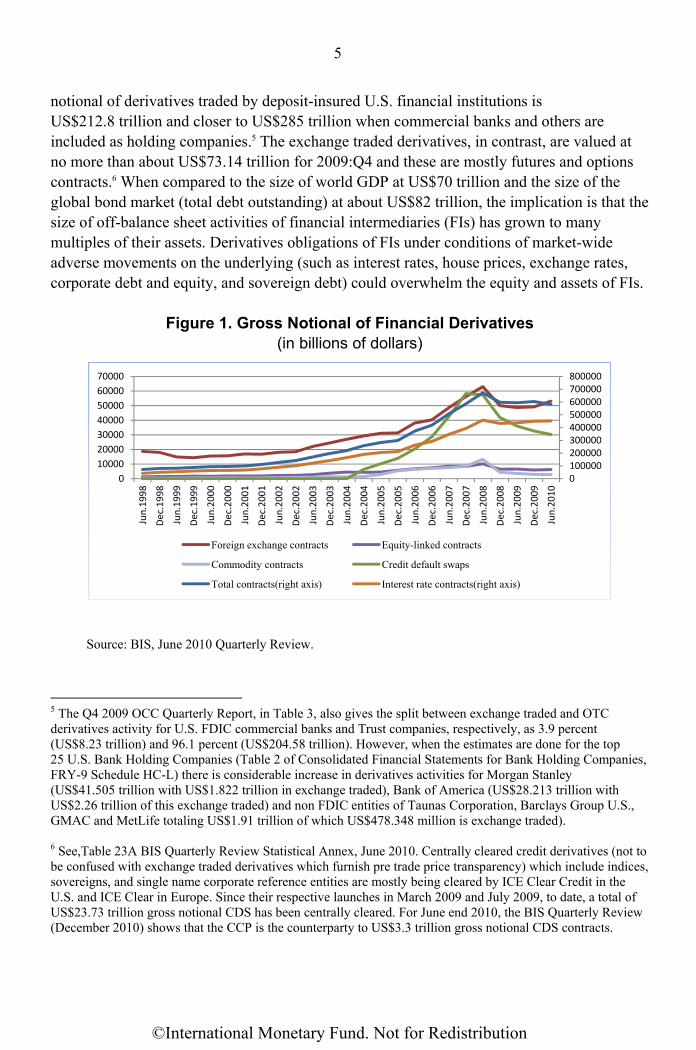
notional of derivatives traded by deposit-insured U.S. financial institutions is US$212.8 trillion and closer to US$285 trillion when commercial banks and others are included as holding companies.5 The exchange traded derivatives, in contrast, are valued at no more than about US$73.14 trillion for 2009:Q4 and these are mostly futures and options contracts.6 When compared to the size of world GDP at US$70 trillion and the size of the global bond market (total debt outstanding) at about US$82 trillion, the implication is that the size of off-balance sheet activities of financial intermediaries (FIs) has grown to many multiples of their assets. Derivatives obligations of FIs under conditions of market-wide adverse movements on the underlying (such as interest rates, house prices, exchange rates, corporate debt and equity, and sovereign debt) could overwhelm the equity and assets of FIs.

Figure 1. Gross Notional of Financial Derivatives (in billions of dollars)

Source: BIS, June 2010 Quarterly Review.

5 The Q4 2009 OCC Quarterly Report, in Table 3, also gives the split between exchange traded and OTC derivatives activity for U.S. FDIC commercial banks and Trust companies, respectively, as 3.9 percent (US$8.23 trillion) and 96.1 percent (US$204.58 trillion). However, when the estimates are done for the top 25 U.S. Bank Holding Companies (Table 2 of Consolidated Financial Statements for Bank Holding Companies, FRY-9 Schedule HC-L) there is considerable increase in derivatives activities for Morgan Stanley (US$41.505 trillion with US$1.822 trillion in exchange traded), Bank of America (US$28.213 trillion with US$2.26 trillion of this exchange traded) and non FDIC entities of Taunas Corporation, Barclays Group U.S., GMAC and MetLife totaling US$1.91 trillion of which US$478.348 million is exchange traded). 6 See,Table 23A BIS Quarterly Review Statistical Annex, June 2010. Centrally cleared credit derivatives (not to be confused with exchange traded derivatives which furnish pre trade price transparency) which include indices, sovereigns, and single name corporate reference entities are mostly being cleared by ICE Clear Credit in the U.S. and ICE Clear in Europe. Since their respective launches in March 2009 and July 2009, to date, a total of US$23.73 trillion gross notional CDS has been centrally cleared. For June end 2010, the BIS Quarterly Review (December 2010) shows that the CCP is the counterparty to US$3.3 trillion gross notional CDS contracts.

0100000200000300000400000500000600000700000800000

0

10000

20000

30000

40000

50000

60000

70000

Jun

.19

98

Dec

.19

98

Jun

.19

99

Dec

.19

99

Jun

.20

00

Dec

.20

00

Jun

.20

01

Dec

.20

01

Jun

.20

02

Dec

.20

02

Jun

.20

03

Dec

.20

03

Jun

.20

04

Dec

.20

04

Jun

.20

05

Dec

.20

05

Jun

.20

06

Dec

.20

06

Jun

.20

07

Dec

.20

07

Jun

.20

08

Dec

.20

08

Jun

.20

09

Dec

.20

09

Jun

.20

10

Foreign exchange contracts Equity-linked contracts

Commodity contracts Credit default swaps

Total contracts(right axis) Interest rate contracts(right axis)


6

Figure 2. Gross Market Values OTC Derivatives (in billions of dollars)

Source: BIS, June 2010 Quarterly Review.

Figures 1 and 2 give the gross notional and the gross market value of the global derivatives in the 5 different derivatives products. Since 2008, there has been a considerable decline in both gross notional and gross market value due to compression and tear ups of bilateral positions. Gross notional is the best measure of the size of derivatives activity and the gross market value gives an estimate of the economic risk in derivatives arising from the volatility of underlying reference/asset prices, leverage and hedge ratios, duration, liquidity, and counterparty risk. Toward, the latter part of 2010, the increase in gross market value of derivatives can be attributed to growing volatility in financial markets. At least since the NBER paper by Darby (1994), risk from financial derivatives has been considered a systemic threat due to the sheer size of the OTC markets and the high concentration of financial obligations. To this may be added the institutional weakness of OTC derivatives market (Duffie, (2010)) and correlated movements (Brunnermeier et. al., (2009)) in the underlying assets of financial derivatives, interest rates, exchanges rates, bank assets, corporate and sovereign debt that can exacerbate the size of derivatives liabilities and also trigger multiple obligations across many sectors. In view of the growing structural concentration in the provision of risk guarantees through financial derivatives, as will be reviewed next, the fragility of the modern risk sharing institutions are germane to issues on systemic risk. Existing statistical models for systemic risk may fail to identify the threats to stability from the topological structures of financial networks often referred to as TITF arising from the concentration of financial links between a few key players. The use of network analysis can help to identify systemically important players in terms of network connectivity, to assess the nature of contagion propagation, and also to monitor and design ways of increasing robustness of the network.

0

5000

10000

15000

20000

25000

30000

35000

40000

0

1000

2000

3000

4000

5000

6000

Foreign exchange contractsEquity-linked contractsCommodity contractsCredit default swapsTotal contracts(right axis)


7

Systemic risk implications of a FI’s connectivity and concentration of obligations, by virtue of being a negative externality, have not been factored into the capital or collateral being held by FIs. Many have remonstrated (Acharya and Richardson (2009), Bernanke (2009)) against the socialization of losses from large complex FIs and have pointed out the need for highly connected FIs to internalize their systemic risk costs. In a ratings based system, as succinctly pointed out by Haldane (2009), leniency of capital and collateral requirements for a few large highly rated financial intermediaries has resulted in excessive expansion of credit and derivatives activities by them that is far beyond what can be sustained in terms of system stability. Further, the expectation that FIs that are TITF will be bailed out also increases their ratings than if this were not to be the case (Moodys (2011), Haldane (2010)). Haldane (2009) calls such highly interconnected FIs ‘super-spreaders’ and this epithet will be retained in the financial network modeling that follows. Haldane (2009) recommends that super-spreaders should have larger buffers. To date, the financial networks literature have produced interesting qualitative analysis for contagion in networks, but have not operationalized a metric for systemic risk for the network system nor a measure of a FI’s contribution to systemic risk arising from the interconnectivity of its financial obligations. This paper is novel in proposing a systemic risk measure directly related to the stability of the financial network topology and a corresponding eigenvector centrality based ‘super-spreader’ tax to reduce the potential socialized losses from failure of highly interconnected FIs in the derivatives markets. Section II will review the data on the derivatives markets to assess the modeling challenges posed by SIFIs (Systemically Important Financial Institutions) that dominate these markets. As the topological fragility arising from TIFT looms large, the extant market data-based methods for estimating systemic risk from FIs will be contrasted with the so called eigen-pair method for financial network stability analysis proposed in this paper. The market data-based methods for systemic risk modeling are found to run into the so called paradox of instability (Borio and Drehmann (2009), Minsky (1982)) that underscores the need to focus on a network model of direct financial exposures and obligations. Section III will review the technical aspects of network theory and economics literature on financial networks. The main drawbacks of the pre-2007 economics literature on financial networks have been that models that are based on empirical bilateral data between counterparties were few in number to establish ‘stylized’ facts on network structures for the different classes of financial products ranging from contingent claims and derivatives, credit related interbank exposures, and large value payment and settlement systems. Where bilateral data on financial exposures were not available, both empirical and theoretical models assumed network structures to be either uncorrelated and random as in Nier et. al. (2007) or complete networks as in Upper and Worms (2004). As will be argued, these approaches crucially do not have the TITF characteristics that will be modelled using a highly sparse core-periphery network structure. Only Craig and von Peter (2010) and Fricke and Lux (2012) who use empirical bilateral interbank data have highlighted the core-periphery network structure that has also been found by the author to be most pronounced in the bilateral data for derivatives liabilities


8

in the Indian financial system.7 While the stability of financial networks has been usually investigated using the classic Furfine (2003) algorithm, sufficient emphasis has not been given to the way in which contagion propagates in highly tiered and clustered networks and stability of the system in terms of network characteristics has not been studied by economists. Following May (1972, 1974) and the recent approach of Wang et. al. (2003) and Giakkoupis et. al. (2005), which is increasingly being adopted in epidemiology and for internet security, the maximum eigenvalue for the network of derivatives liabilities expressed as a ratio of Tier 1 capital will be used to determine the stability of the system. Section IV discusses the necessary network stability results using maximum eigenvalue and the corresponding eigenvector centrality of the FIs. Systemic risk index for each FI is based on its right eigenvector centrality and the super-spreader tax fund that can mitigate potential socialized losses from the failure of highly connected banks is designed. In contrast, the left eigenvector centrality index for the financial network will be called the vulnerability or exposure index. In the empirical Section V, the empirical reconstruction of the derivatives network based on 2009:Q4 data is undertaken and the network analysis and a series of stress tests are conducted to investigate the consequences of the high concentration of activity of 12 or so SIFIs. The super-spreader tax is quantitatively derived and back tested to see if sufficient funds are escrowed from the super-spreader tax generated to stabilize the system. Section VI concludes the paper and outlines future work.

II. SYSTEMIC RISK IN OTC DERIVATIVES: MODELING CHALLENGES

A. SIFIs in Derivatives Markets and Market Concentration

Typically, risk sharing in advanced financial systems is accomplished by OTC derivatives. At the level of the individual user, these schemes appear plausible as a means of risk shifting, but at the macro-level they may lead to systemically unsustainable outcomes as interconnectivity of FIs increases. The success of risk sharing at a system level is crucially related to the numbers of protection sellers or those who have a considerable position in derivatives liabilities and the structural interconnections involved in the provision of guarantees. Indeed, the key structural aspect of the networks underpinning financial derivatives has been summarized in the 2009 Fitch survey: “dependence on a limited number of counterparties looks to be a permanent feature of the market; this is underscored by the fact that the top 12 counterparties comprised 78 percent of total exposure in terms of the number of times cited, up from the 67 percent reported last year. 8,9 The top five institutions

7 See Reserve Bank of India Financial Stability Report, December 2011.

8 http://www.scribd.com/doc/37557210/Fitch-Market-Research-Global-Credit-Derivatives-Survey-09162010.

9 The 12 counterparties are Goldman Sachs, JP Morgan Chase, Barclays, Bank of America, Deutsche Bank, Morgan Stanley, Credit Suisse, BNP Paribas, UBS, Merrill Lynch, and Royal Bank of Scotland.


http://www.scribd.com/doc/37557210/Fitch-Market-Research-Global-Credit-Derivatives-Survey-09162010

9

that provided volume figures accounted for 95 percent of total notional amount bought and sold. This concentration is a reflection of the dominant role of banks and dealers as counterparties, particularly after the collapse of a limited number of financial institutions who were important intermediaries in this market.” In an attempt to address systemic risk in the financial system, the notion of a Systemically Important Financial Institution (SIFI) has come to the forefront. Joint statements by the Financial Stability Board, IMF and BIS have identified these FIs in regard to large size, prominence in markets or functions (non-substitutability), complexity, global activity and interconnectedness. 10 It is important that some metric for systemic risk based upon the impact of a firm’s failure on the financial system as a whole is found and that some figures for extra capital charges have already been stipulated to range from one percent to 2.5 percent depending on the assessment of the above factors for SIFIs, with an additional one-percent capital charge levied on institutions considered to be very risky. The question is: can SIFIs internalize their systemic risk costs arising from their activities in specific sectors and markets with a non-specific capital surcharge? In what way can the surcharge be attributable to a SIFI’s strategies, for instance, in global derivatives markets that have been a cause for concern? This study involves 202 participants of derivatives markets based in the U.S. and Europe, of which 20 institutions are global SIFIs while other 18 institutions are broker dealers in over four of the five derivatives markets. Using an affiliation graph in Figure 3 on the number of participants in each of the derivatives products, the dominance of 8 broker dealers can be seen in the centre of Figure 3. The majority of 126 institutions belong to only 1 product market, 23 to two products only, 8 to three, 10 to four, and 8 to all five markets. Affiliations to only one market are arranged at the outer corners of the graph in Figure 3, those in any 2 markets are arranged further in from the edges and the most central circle consists of the 8 broker dealers in all 5 markets surrounded by those that are present in 4 markets. It is important to study the systemic risk from activities of SIFIs and other FIs in the different derivatives markets to fully understand the propagation of financial contagion that often emanates from specific markets and underlying assets (e.g., mortgage backed securities in the CDS market, Markose et. al. (2012)). With interest rates at a historic low, serious concerns are warranted about the systemic risk from interest rate swaps that account for over 80 percent of financial derivatives. However, the starting point of this study is the calibrated network of bilateral assets and liabilities that the 202 FIs face in respect to derivatives contracts aggregated over all derivatives products.

10 See http://www.financialstabilityboard.org/publications/r_111104bb.pdf.


http://www.financialstabilityboard.org/publications/r_111104bb.pdf

10

Figure 3. Affiliation Graph of Global SIFIs and United States (U.S.) FDIC FIs as Participants in the Five Financial Derivatives Markets

Note: Total number of participants is 202 based on gross notional data for Forex (Blue: 48), Interest Rate Swaps (Green: 189), Equities (Brown: 25), Commodities and others (Yellow: 22), CDS (Red: 23). Source: Data on non U.S. FIs and global U.S SIFIs (see footnote 8) is from individual 2009 Annual Financial Statements; remaining U.S. FIs’ data from FDIC Call Reports Q4 2009. The data are summarized in Table 1.11 As discussed in the OCC Quarterly Report (2009), the first step in measuring credit exposure in derivatives contracts is to identity the contracts that would lead a FI to lose value if the counterparty to the contract defaults. The contracts with gross positive fair value (GPFV) for a FI constitute the derivatives receivables from its counterparties without taking into account netting. Where no legally binding bilateral netting exists between a FI and its counterparties and the FI receives no collateral from them, GPFV is the maximum credit exposure or losses a FI will face if its counterparties fail. In turn, a FI’s derivatives contracts with a negative fair value, with no netting and no collateral posted by the FI to its counterparties, represents gross negative fair value (GNFV) or the total derivatives payables to the FI’s counterparties. The fair values are obtained from the market price of the instrument if it is traded or model determined if it is not

11 Data for the top 20 FIs are given in the Appendix.


11

traded. Derivatives liabilities and derivatives assets are respectively estimated once the gross payables and gross receivables for each FI are adjusted for collateral and bilaterally netted on a multi-product basis where master agreements exist and summed over all counterparties. The derivatives assets are the amounts that matter as the loss given default of a FI’s counterparties and they attract a Basel II capital charge. Regulators such as the U.S. Office of Comptroller of the Currency (see OCC Quarterly Derivatives Trading Reports) have resorted to an aggregate metric called net current credit exposure (NCCE) to evaluate credit risk in banks’ derivatives activities that is based on derivatives assets. However, as first noted by Singh (2010) “a FI’s derivative payables is the risk imposed on the rest of counterparties when it fails” and this represents the causal factor for a FI’s systemic risk from its activities in the derivatives markets. Hence, in what follows, the focus will be on the network of derivatives liabilities and a systemic risk surcharge on FIs will be determined on the basis of their interconnectivity and centrality in the system from the direction of liabilities of FIs.12

Table 1. Value and Market Share of Financial Derivatives for 202 FIs (in trillions of dollars)

All FIs Top 16 FIs Top 26 FIs

Gross Notional 674.369 659.263 (97.76%)

673. 827 (99.92%)

Gross Positive Fair Value (GPFV) 10.465 10.254 (97.98%)

10.453 (99.89%)

Gross Negative Fair Value (GNFV) 10.144 9.934 (97.92%)

10.134 (99.89%)

Derivatives Assets 1.168

1.068 (91.39%)

1.15 (98.52%)

Derivatives Liabilities 0.889

0.816 (91.78%)

0.874 (98.33%)

Total Assets 37.252 27.863

(74.80%)

32.837 (88.15%)

Tier 1 capital 1.413 1.014 (71.60%)

1.207 (85.48%)

Source: Data on non U.S FIs and global U.S SIFIs (see footnote 8) from individual 2009 Annual Financial Statements; remaining U.S FIs’ data from FDIC Call Reports Q4 2009.

Note: The market shares are in parenthesis.

Table 1 highlights two aspects of systemic risk characterizing derivatives market: the unique and dominant role played by SIFIs and the large size of derivatives assets and liabilities relative to Tier 1 capital of the sector. Further, as the underlying of financial derivatives is pro-cyclical to macro-economic factors and guarantors of credit risk are caught

12 The Dodd-Frank Act has included derivatives liabilities in excess of US$3.3 billion on the list of criteria signalling systemic risk of a non-bank financial company, www.treasury.gov/press-center/press-releases/Pages/tg1580.aspx . This insight has been kindly provided by Manmohan Singh.


www.treasury.gov/press-center/press-releases/Pages/tg1580.aspx

www.treasury.gov/press-center/press-releases/Pages/tg1580.aspx

12

up in a self-reflexive loop, this can promote an excessive growth of these derivatives that may appear rational at the level of the individual unit.13 However, far from mitigating volatility, derivatives growth can bring about extreme tail events for which the financial system will be unable to provide protection in regard to settlement liquidity (Brock et. al. (2009), Rajan (2006)). Not present in Table 1 are the data that show smaller end-user hedge benefits are supported by larger offsetting activities done by broker dealers of derivatives in which a large proportion of payoffs at settlement goes to speculative ‘naked’ buyers of derivatives.14 The dislocation here is that financial derivatives trading provide greater profitability to broker-dealers in the short run than returns from real side investment.

B. Market Data Based Systemic Risk Measures and Financial Network Perspective

In contrast to the approach taken in this paper, by and large, systemic risk models have relied on statistical market price based data to extrapolate from the micro-prudential risk measures of Basel II to obtain macro-prudential measures. To analyze so called interconnectedness risk between FIs, matrix of bilateral correlations or non-linear copula based co-movements purported to represent extreme market conditions is constructed. The main market-based systemic risk measures that have been proposed are Conditional VaR (CoVaR) by Adrian and Brunnermeier (2009), System Expected Shortfall (SES) by Acharya et al. (2010), Co-risk by Chau-Lan (2010), DIP (Distress Insurance Premium) by Huang et al. (2010), POD (Probability that at least one bank becomes distressed) by Segoviano and Goodhart (2009), Shapley-Value by Tarashev et. al. (2010) and Macro-prudential capital by Gauthier et. al (2009). The ingredients of most statistical systemic risk measures involve the following. Firstly, a system wide expectation is formed of joint extreme/tail losses on a debt/liability or equity portfolio of all FIs (joint portfolio) often using VaR or Expected Shortfall type measures. The systemic risk of a FI is then estimated in a number of ways: a simple beta statistic (ratio of covariance of tail loss of FI to the variance of the joint portfolio tail loss); the marginal contribution given as expected loss of the FI conditional on the joint portfolio loss (Huang et. al. (2010)); as ‘incremental’ (-CoVaR) joint portfolio tail loss conditional on the default of the FI less the joint portfolio tail loss conditional of the FI being solvent; or using the Myerson-Shapley value that, in a network setting with a number (N) of FIs, requires the

13 Reflexivity refers to fixed point mappings that include wrong way risk—CDS protections providers themselves get downgraded as conditions on the credit risk on underlying deteriorates— and can exacerbate tail risk that derivatives are meant to mitigate. Fitch Ratings’ Global Credit Derivatives Surveys and 2009 Depository Trust and Clearing Corporation (DTCC) data on outstanding contracts on reference entities show that seven broker-dealers in derivatives markets have moved up the ranks in the top 25 reference entities in CDS markets with many of them providing protection on others. 14 Graph 5B of OCC Quarterly Report on Bank Trading and Derivatives Q4 2009 shows that there has been an increased growth of netting benefits relative to the growth in gross notional value of derivatives contracts. See also Das (2010).


13

incremental risk measure to be evaluated over all non-zero subgraphs of N.15 The principle is that capital surcharge or macro-prudential capital requirement for each FI should reflect the FI’s contribution to the joint portfolio loss. Chan-Lau (2010), for instance, specifies the systemic risk surcharge for a FI as the product of an incremental social loss function and the probability of default of the FI. In those systemic risk measures that aim to estimate the joint portfolio loss, the probability of default (PoD) of a FI and a matrix of pairwise conditional PoDs are needed. There are many methods to determine the PoD of an FI. Popular among them is to use CDS spreads directly to proxy PoDs, back them out from CDS spreads or use default estimates from data providers such as Moody’s KMV. The conditional pairwise PoD is obtained by (high at 95) quantile regressions of one FI’s PoD on that for another FI and common risk factors (Chan-Lau (2010)). The Segoviano and Goodhart (2009) banking stability index is based on a similarly constructed distress dependence matrix. They then use the probability of one or more FIs being in distress conditional on a particular FI being the trigger to determine the systemic risk impact of the FI. The major drawback of market price data based measures of systemic risk is that they can suffer from the paradox of financial instability (Borio and Drehmann (2009)) or the paradox of volatility, issues first addressed by Minsky (1982).16 These market price-based statistical proxies for market risk (volatility index) and credit risk (CDS spreads) are at their lowest just before the point of great financial collapse and hence, while there may be information in the cross-sectional data of FI’s contributions to systemic risk, the aggregated market price-based systemic risk statistics are at best contemporaneous with the crisis in markets.17 In fact, Castren and Kovonius (2009) show that their distance to distress (DD) systemic risk measure with a high DD signaling low distress “dropped sharply only after 15 See Kirman et. al. (2007) for a discussion on the dimensionality (NP-hard) problem that the use of Myerson-Shapley principle entails when sub-networks are selected instead of sub-groups.

16On the paradox of financial instability, Borio and Drehmann (2009) state that "the financial system looks strongest when it is most fragile." As this also corresponds to the relationship between a publicly available volatility index, such as the VIX, and the underlying stock price index, it has led to the notion of the paradox of volatility. The volatility index, often taken as a proxy for market risk, is typically low during bull market conditions. The paradox is that it experiences its lowest point when the market index is at its highest point prior to an extreme fall. As credit growth boosts asset prices, CDS spreads are also inversely related to asset prices and are at their lowest precisely before the crash when asset prices peak. Hence, market data paradoxically signals least risk just before a major market collapse! The Minsky (1982) thesis is a more general one in that it holds that the seeds of financial collapse are sown during the boom asset market conditions that mask the excessive growth of leverage and financial fragility.

17 At the 2010 IMF Workshop on Operationalizing Systemic Risk, Markose showed that the Segoviano-Goodhart (2009) Banking Stability Index and the volatility indexes VIX or VFTSE spiked contemporaneously with the 2007 crisis. These indexes all also subsided far too soon after the Lehman Brother crisis, blunting their efficacy as an early warning signal for impending and prolonged financial market crisis. Rama Cont expressed similar concerns.


14

(italics added) the crisis had started.” They claim that the high DDs “in the years 2005–2006 were mainly driven by historically low volatility … even though from the market leverage Chart 6, it is clear that vulnerabilities were gradually accumulating in the form of rising indebtedness in most sectors.” Adrian and Brunnermeir (2009) have directly incorporated information on banks’ balance sheet and financial liabilities/leverage to overcome pro-cyclicality of market price data in systemic risk indexes that lead them to obscure the growing risk from leverage. Thus, while Adrian and Brunnermeir (2009) do address the paradox of financial instability problem by proposing a countercyclical forward Co-Var measure, this is not the case with most market price based systemic risk measures. 18 Note that, after the regime has changed to the high volatility state, the market-based systemic risk measures are good at capturing the direction of the contagion from increased statistical cross correlation in the falling asset returns. To date there has been no comprehensive study of TITF and systemic risk measures based on the network topology of bilateral exposures and obligations specifically for derivatives markets. Financial network models based on financial exposures are models that aim to depict causal chains of exposures and obligations of counterparties rather than rely solely on statistical correlations on market price-based data for FIs. The only quantitative assessment to date of FIs’ overall derivatives liabilities and systemic risk impact is that of Segoviano and Singh (2008). The paper is based on the FDIC/OCC data on fair value of derivatives liabilities for FIs and the CDS spreads for these FIs as reference entities. The latter determines the conditional default probabilities and the so called distress dependence between FIs determines which FIs will fail conditional on failure of others. Under post crisis bear market conditions, market price data show increased correlations and co-movements in the adversely affected financial market sector. Segoviano and Singh (2008) find that the expected cumulative derivatives losses when cascaded in a series of insolvencies of top broker dealers exceed the capabilities of the Fed Reserve to provide backstops. This adds urgency for the need to conduct an in-depth structural analysis of the financial derivatives and the role of large FIs. In contrast to the Segoviano-Singh framework where cascade effects are governed by the distress matrix based on the CDS spreads on the FIs, in the financial network model the direction and magnitude of derivatives payables and receivables between FIs govern connectivity, concentration, network structure and system instability. The Markose et. al. (2012) network algorithm based on market shares of FIs and others in the gross negative (positive) fair value of the derivatives contracts determines the ranking in the market for network links from (to) each FI and hence also the bilateral links between agents.

18 To reverse the procyclicality of market price-based systemic risk measures, Adrian and Brunnermeir (2009) in the forward Co-VAR include panel data on lagged FI specific characteristics such as size, leverage, maturity mismatch, etc. This supplemented quantile regressions for forward Co-Var was found to be inversely related to the systemic risk measure based on market price data alone.


15

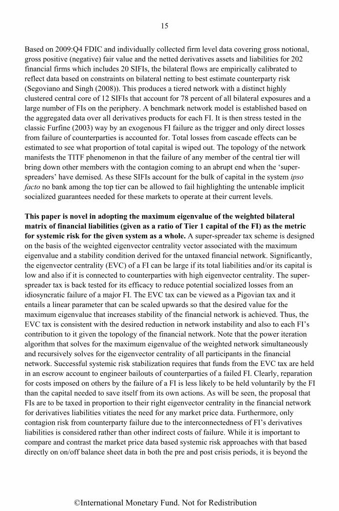
Based on 2009:Q4 FDIC and individually collected firm level data covering gross notional, gross positive (negative) fair value and the netted derivatives assets and liabilities for 202 financial firms which includes 20 SIFIs, the bilateral flows are empirically calibrated to reflect data based on constraints on bilateral netting to best estimate counterparty risk (Segoviano and Singh (2008)). This produces a tiered network with a distinct highly clustered central core of 12 SIFIs that account for 78 percent of all bilateral exposures and a large number of FIs on the periphery. A benchmark network model is established based on the aggregated data over all derivatives products for each FI. It is then stress tested in the classic Furfine (2003) way by an exogenous FI failure as the trigger and only direct losses from failure of counterparties is accounted for. Total losses from cascade effects can be estimated to see what proportion of total capital is wiped out. The topology of the network manifests the TITF phenomenon in that the failure of any member of the central tier will bring down other members with the contagion coming to an abrupt end when the ‘super-spreaders’ have demised. As these SIFIs account for the bulk of capital in the system ipso facto no bank among the top tier can be allowed to fail highlighting the untenable implicit socialized guarantees needed for these markets to operate at their current levels. This paper is novel in adopting the maximum eigenvalue of the weighted bilateral matrix of financial liabilities (given as a ratio of Tier 1 capital of the FI) as the metric for systemic risk for the given system as a whole. A super-spreader tax scheme is designed on the basis of the weighted eigenvector centrality vector associated with the maximum eigenvalue and a stability condition derived for the untaxed financial network. Significantly, the eigenvector centrality (EVC) of a FI can be large if its total liabilities and/or its capital is low and also if it is connected to counterparties with high eigenvector centrality. The super-spreader tax is back tested for its efficacy to reduce potential socialized losses from an idiosyncratic failure of a major FI. The EVC tax can be viewed as a Pigovian tax and it entails a linear parameter that can be scaled upwards so that the desired value for the maximum eigenvalue that increases stability of the financial network is achieved. Thus, the EVC tax is consistent with the desired reduction in network instability and also to each FI’s contribution to it given the topology of the financial network. Note that the power iteration algorithm that solves for the maximum eigenvalue of the weighted network simultaneously and recursively solves for the eigenvector centrality of all participants in the financial network. Successful systemic risk stabilization requires that funds from the EVC tax are held in an escrow account to engineer bailouts of counterparties of a failed FI. Clearly, reparation for costs imposed on others by the failure of a FI is less likely to be held voluntarily by the FI than the capital needed to save itself from its own actions. As will be seen, the proposal that FIs are to be taxed in proportion to their right eigenvector centrality in the financial network for derivatives liabilities vitiates the need for any market price data. Furthermore, only contagion risk from counterparty failure due to the interconnectedness of FI’s derivatives liabilities is considered rather than other indirect costs of failure. While it is important to compare and contrast the market price data based systemic risk approaches with that based directly on on/off balance sheet data in both the pre and post crisis periods, it is beyond the


16

scope of this paper to do so.

III. FINANCIAL NETWORK ANALYSIS

Networks are defined by a pair of sets (N, E) that stand for the finite set of nodes N={1,2,3,…..,n}, and E is a set of edges. In financial networks nodes stand for financial entities such as banks, other financial intermediaries, and their non-financial customers. The edges or connective links represent contractual flows of liquidity and/or obligations to make payments and receive payments. Let i and j be two members of the set N. When a direct link originates with i and ends with j, viz. an out degree for i, it represents payments for which i is the guarantor. Note that an agent’s out degrees correspond to the number of its immediate neighbours or counterparties and is denoted by ki. A link from j to i yields an in degree for i and represents cash inflows or financial receivables for i from j.

A. Adjacency Matrix and Gross Flow Matrix for Derivatives

Key to the network topology is the bilateral relations between agents and is given by the adjacency matrix. Denote the (N +1) x (N +1) adjacency matrix A = (aij)

I , here I is the indicator function with aij = 1 if there is a link between i and j and aij = 0, if not. The Nth agent will be represented by the non-bank FIs such as Monolines, hedge funds and insurance companies. The N+1th agent represents participants not including the 202 U.S. and European FIs. This is also used to balance the system. The set of agent i’s ki direct neighbours i = { j, j i, such that aij = 1} gives the list of i’s counterparties to whom which i has to make payments or fulfil other financial obligations. The adjacency matrix becomes the gross flow matrix X such that xij represents the flow of gross financial obligations, GNFV, from the derivatives seller (the row FI) to the derivatives buyer j (the column FI). Note that GNFV and GPFV are a fraction (typically 10 percent) of the gross notional for which the firm is a derivatives seller or buyer, respectively. The total gross payables in terms of GNFV for FI i is the sum over j columns or counterparties, Gi = ∑ while the total gross receivables or

total GPFV for each j is the sum taken across the i rows Bi = ∑ . This is shown below:

X =

NBBBB

G

G

G

G

G

xx

xx

xxx

xxxx

Njj

j

N

i

ii

jNN

iNi

N

Nij

11

1

2

1

111

11

122321

111312

......

.

.

0.....

0...

0..

.........0..

........0

.......0

(1)


17

The zeros along the diagonal imply that FIs do not lend to themselves (see, Upper, 2007) or and in case of contagion, FIs do not ‘infect’ themselves. There can be asymmetry of entries such that for instance G1 need not equal B1. However, aggregate GNFV including that of the

N+1 entity i

iG will be made to balance with the .j

jB

B. Bilaterally Netted Matrix of Payables and Receivables

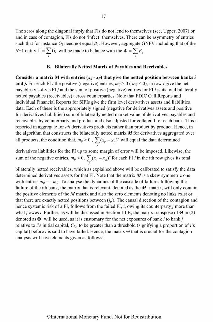
Consider a matrix M with entries (xij - xji) that give the netted position between banks i and j. For each FI i the positive (negative) entries, mij > 0 ( mij < 0), in row i give the net payables vis-à-vis FI j and the sum of positive (negative) entries for FI i is its total bilaterally netted payables (receivables) across counterparties. Note that FDIC Call Reports and individual Financial Reports for SIFIs give the firm level derivatives assets and liabilities data. Each of these is the appropriately signed (negative for derivatives assets and positive for derivatives liabilities) sum of bilaterally netted market value of derivatives payables and receivables by counterparty and product and also adjusted for collateral for each bank. This is reported in aggregate for all derivatives products rather than product by product. Hence, in the algorithm that constructs the bilaterally netted matrix M for derivatives aggregated over

all products, the condition that, mij > 0 , j

jiij xx )( will equal the data determined

derivatives liabilities for the FI up to some margin of error will be imposed. Likewise, the

sum of the negative entries, mij < 0, j

jiij xx )( for each FI i in the ith row gives its total

bilaterally netted receivables, which as explained above will be calibrated to satisfy the data determined derivatives assets for that FI. Note that the matrix M is a skew symmetric one with entries mij = - mji. To analyse the dynamics of the cascade of failures following the failure of the ith bank, the matrix that is relevant, denoted as the M+ matrix, will only contain the positive elements of the M matrix and also the zero elements denoting no links exist or that there are exactly netted positions between (i,j). The causal direction of the contagion and hence systemic risk of a FI, follows from the failed FI, i, owing its counterparty j more than what j owes i. Further, as will be discussed in Section III.B, the matrix transpose of Θ in (2) denoted as ´ will be used, as it is customary for the net exposures of bank i to bank j relative to i’s initial capital, Ci0, to be greater than a threshold (signifying a proportion of i’s capital) before i is said to have failed. Hence, the matrix Θ that is crucial for the contagion analysis will have elements given as follows:


18

)2(

0...)(

....)(

.0........

)(...0....

)(.........0..

)(........

)(00

0....0)()(

0

010

11

010

11

0

33

30

3223

30

3113

20

2112

j

jNNjNN

N

NiiNii

N

NN

C

xx

C

xx

C

xx

C

xx

C

xx

C

xxC

xx

C

xx

The matrix Θ is a non-negative real matrix as no element is negative and all elements are either zero or strictly positive real numbers, . . , 0. In general, a matrix or vector will

be said to be positive (non-negative) if all elements in it are positive (non-negative).

C. Topology of Financial Networks Complete, Random, Core-periphery, Clustered, and Small World

Like many real world socio-economic, communication, and information networks such as the www, financial networks are far from random and uncorrelated. In order to construct and characterize financial networks that have high concentration or localization of exposures with dense network interconnectivity between a few FIs, it is useful to briefly survey the well known classification of networks (see Table 2) and highlight the properties of small world networks that are a good fit for the financial network of exposures found in derivatives markets.19 The aim is to incorporate the highly skewed connectivity of 26 broker-dealers representing high concentration of derivatives liabilities in Table 1. This implies that other participants who are in the majority have little or no links to one another and instead are linked to the central core. Thus, a core-periphery structure (Borgatti and Everett, 1999) with small world network properties manifests itself in the derivatives network. This has also been regarded to be a statistical signature of complex social systems (Watts(1998) and Watts and Strogatz (1999)) namely, a top tier multi-hub of few agents who are highly connected among themselves (often called rich club dynamics) and to some other nodes in the periphery who show few if any connections amongst themselves. The properties of small world networks and how contagion propagates through them will be briefly contrasted with that for

19 Small world networks are named after the work of Stanley Milgram (1967) on the six degrees of separation in social networks. It has been found that globally, on average, everybody is linked to everybody else by no more than six indirect links.


19

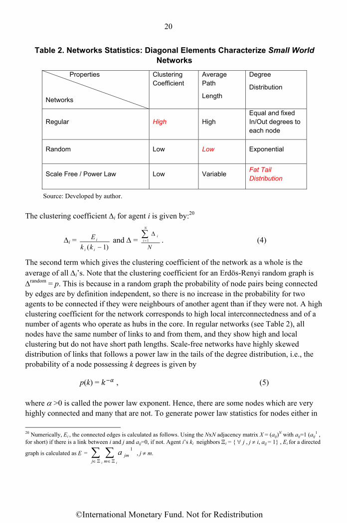
the Erdös-Renyi random graph and also the Barabási and Albert (1999) scale free networks. In order to construct a network for financial derivatives that shows dominance of few players with a 92 percent and upwards of concentration of derivatives exposures to one another, use will be made of network statistics and dynamics described below regarding high clustering, preferential attachment in link formation, and identification of members with high ‘rich club’ statistics. Networks are mainly characterized by a set of network statistics. These are: (i) the probability of any two randomly selected nodes in a network being connected is denoted by p with there being total of N(N-1) possible links for directed graphs and N(N-1)/2 for undirected graphs; (ii) measure of local interconnectivity between nodes called clustering coefficient (i denotes the clustering coefficient for node i and is the clustering coefficient for the network); (iii) the shortest path length of the network estimates the average shortest path between all pairs of randomly selected nodes; and (iv) degree distribution that gives the probability distribution P(k) as a function of the degrees k of each of the nodes, and p(k) gives the probability that a randomly selected node as exactly k links. The average number links per node is given by <k> = kk p(k) and the variance of links <k2> = kk

2 p(k). Where empirical sample data is used, p(k) = Nk/N-1 where Nk is the number of nodes with k links. Textbook prototypes of regular, random, and scale-free networks have properties in respect to the network statistics given in Table 2. As will be explained, small world networks described by elements along the diagonal of Table 2 have one property in common with each of the other network types. In Erdös-Renyi random networks in which connectivity between any two nodes is uncorrelated, the probability distribution of degrees is given by:

P(k) = 1 1

! . (3)

The exact solution to the last term above is achieved in the limit when N→∞. The Erdös-Renyi random networks show little local interconnectivity or clustering. They have short path lengths due to the random link formation. The average shortest path between any two arbitrarily chosen nodes is found to be “small” and bounded by the logarithm of the total number of nodes in the system. Clustering in networks measures how interconnected each agent’s neighbours are and is considered to be the hallmark of social and species-oriented networks. Specifically, there should be an increased probability that two of an agent’s neighbours are also neighbours of one another. For each agent with ki neighbours the total number of all possible directed links between them is given by ki (ki-1). Let Ei denote the actual number of links between agent i’s ki neighbors, viz. those of i’s ki neighbours who are also neighbours.


20

Table 2. Networks Statistics: Diagonal Elements Characterize Small World Networks

Source: Developed by author.

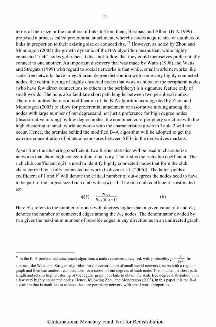
The clustering coefficient i for agent i is given by:20

i = )1( ii

i

kk

E and = N

N

ii

1 . (4)

The second term which gives the clustering coefficient of the network as a whole is the average of all i’s. Note that the clustering coefficient for an Erdös-Renyi random graph is random = p. This is because in a random graph the probability of node pairs being connected by edges are by definition independent, so there is no increase in the probability for two agents to be connected if they were neighbours of another agent than if they were not. A high clustering coefficient for the network corresponds to high local interconnectedness and of a number of agents who operate as hubs in the core. In regular networks (see Table 2), all nodes have the same number of links to and from them, and they show high and local clustering but do not have short path lengths. Scale-free networks have highly skewed distribution of links that follows a power law in the tails of the degree distribution, i.e., the probability of a node possessing k degrees is given by

p(k) = , (5) where >0 is called the power law exponent. Hence, there are some nodes which are very highly connected and many that are not. To generate power law statistics for nodes either in

20 Numerically, Ei , the connected edges is calculated as follows. Using the NxN adjacency matrix X = (aij)

N with aij=1 (aij1 ,

for short) if there is a link between i and j and aij=0, if not. Agent i’s ki neighbors i = { j , j i, aij = 1} , Ei for a directed

graph is calculated as E = i ij m

jma 1 , j m.

Properties

Networks

Clustering Coefficient

Average Path

Length

Degree

Distribution

Regular High High Equal and fixed In/Out degrees to each node

Random Low Low Exponential

Scale Free / Power Law Low Variable Fat Tail Distribution


21

terms of their size or the numbers of links to/from them, Barabási and Albert (B-A,1999) proposed a process called preferential attachment, whereby nodes acquire size or numbers of links in proportion to their existing size or connectivity. 21 However, as noted by Zhou and Mondragon (2003) the growth dynamic of the B-A algorithm means that, while highly connected ‘rich’ nodes get richer, it does not follow that they could themselves preferentially connect to one another. An important discovery that was made by Watts (1998) and Watts and Strogatz (1999) with regard to social networks is that while, small world networks like scale-free networks have in-egalitarian degree distribution with some very highly connected nodes, the central tiering of highly clustered nodes that work as hubs for the peripheral nodes (who have few direct connections to others in the periphery) is a signature feature only of small worlds. The hubs also facilitate short path lengths between two peripheral nodes. Therefore, unless there is a modification of the B-A algorithm as suggested by Zhou and Mondragon (2003) to allow for preferential attachment or assortative mixing among the nodes with large number of out degreesand not just a preference for high degree nodes (disassortative mixing) by low degree nodes, the combined core-periphery structure with the high clustering of small world networks with the characteristics given in Table 2 will not occur. Hence, the premise behind the modified B–A algorithm will be adopted to get the extreme concentration of bilateral exposures between SIFIs in the derivatives markets.

Apart from the clustering coefficient, two further statistics will be used to characterize networks that show high concentration of activity. The first is the rich club coefficient. The rich club coefficient, k) is used to identify highly connected nodes that form the club characterized by a fully connected network (Colizza et. al. (2006)). The latter yields a coefficient of 1 and k# will denote the critical number of out-degrees the nodes need to have to be part of the largest sized rich club with k) = 1. The rich club coefficient is estimated as:

k) = . (6)

Here N>k refers to the number of nodes with degrees higher than a given value of k and E>k denotes the number of connected edges among the N>k nodes. The denominator divided by two gives the maximum number of possible edges in any direction as in an undirected graph.

21 In the B–A preferential attachment algorithm, a node i receives a new link with probability pi =

∑. In

contrast, the Watts and Strogatz algorithm for the construction of small world networks, starts with a regular graph and then has random reconnections for a subset of out degrees of each node. This obtains the short path length and retains high clustering of the regular graph, but fails to obtain the scale free degree distribution with a few very highly connected nodes. Hence, following Zhou and Mondragon (2003), in this paper it is the B-A algorithm that is modified to achieve the core-periphery network with small world properties.


22

The network centrality measure that has been found by the author to correlate best with the capacity of a FI to cause the largest contagion losses on others in the Furfine (2003) type stress test is its eigenvector centrality statistic obtained for matrix in equation (2). The algorithm that determines it assigns relative centrality scores to all nodes in the network based on the principle that connections to high-scoring nodes contribute more to the score of the node in question than equal connections to low-scoring nodes. Denoting as the right eigenvector centrality for the ith node for matrix , the centrality score is proportional to the sum of the centrality scores of all nodes to which it is connected (i.e., ki

neighbours). Hence,

= ∑ . (7)

For the centrality measure in (7), the largest eigenvalue, λmax , and its associated eigenvector are taken. The ith component of this eigenvector then gives the centrality score of the ith node in the network. Using vector notation, the eigenvalue equation for the matrix in (2) for the eigen-pair (λmax, ) is given as:

= λmax . (8.a)

Note that for a non-negative matrix in (2) with real entries, λmax is a real positive number and the eigenvector associated with the largest eigenvalue has non-negative components by the Perron-Frobenius theorem (see Meyer (2000), Chapter 8). Positive values for the centralities of all nodes of matrix in (2) are guaranteed by Perron-Frobenius theorem only if in (2) is irreducible.22 For matrix clearly, given equation (7), those nodes in the periphery with no out-degrees will have zero eigenvector centrality. Finally, from the perspective of the measure of systemic risk, the so called right eigenvector of matrix given above in (8.a), as will be discussed, is what matters. A FI’s systemic risk index will be based on this. It measures the impact of FIs’ total liabilities relative to the respective capital of each of its counterparties given by the row sums of matrix in (2) on the stability of the system characterized by the maximum eigenvalue. The so-called dual left eigenvector, on the other hand, gives the impact of the exposures of each FI to others and hence can be seen to yield vulnerability indices. The left eigenvector of denoted by v1 is defined as

v1 = ´v1 = λmax v1 . (8.b)

22 The condition of the Perron-Frobenius theorem that guarantees a positive eigenvector corresponding to the maximum eigenvalue for the non-negative matrix is that the directed graph it represents should be irreducible. That is, for any randomly selected pairs of nodes (i,j) there is a path between them, viz. is strongly connected, Meyer (2000).


23

Note both the left and right eigenvectors yield the same maximum eigenvalue for the matrix in (2).23

D. Economics Literature on Financial Networks

Pre-2007 financial network models in the economics literature have yielded mixed results. An influential and early work on connectivity in a financial network and that of financial contagion is that of Allen and Gale (2001). They gave rise to a mistaken view that follows only in the case of homogenous graphs, i.e., increasing connectivity monotonically increases system stability in the context of diversification of counterparty risk.24 Battiston et al. (2010) have correctly shown that connectivity and stability of a network is not a simple monotonic relationship but that beyond a point, connectivity in a network could increase instability. However, Battiston et al. (2010) do not offer insights into what sort of network topologies give rise to concerns about financial intermediaries being TITF either. Indeed, the derivatives-based risk sharing networks, as discussed above, need to be characterized by highly interconnected central tier composed of high degree hub nodes that have been called rich clubs. In contrast, the bulk of numerically based studies in financial contagion work (Nier et al. (2007) and Gai and Kapadia (2010)) has been confined to Erdös-Renyi random graphs and while they can be regarded as first steps, as financial networks are far from random, they have some way to go.

As little empirical work has been done to date on network structures of the specific markets underpinning off-balance sheet bank activity such as CDS responsible for triggering and propagating the 2007 crisis, it must be noted that the bulk of the empirical financial network approach has been confined to interbank credit markets for their role in the spread of financial contagion (see Furfine (2003) and Upper (2007)). However, the use of the entropy method (Upper and Worms (2004) and Boss et al. (2004)) for the construction of the matrix of bilateral obligations of banks that results in a complete and as homogenized network structure as possible, greatly vitiates the potential for network instability or contagion.25

Recent work by Craig and von Peter (2010) using bilateral interbank data from German banks and also by Fricke and Lux (2012) for the Italian interbank market has

23 Fujiwara et. al. (2009) have also noted the significance of the right and left eigenvectors to provide centrality indices for banks and firms in a birpartite graph of lending relationships between banks and firms in Japan.

24 In a complete graph, if bank i’s total exposure is equally divided among its N-1 counterparties, then risk is shared equally at the rate of 1/N-1. The demise of a single counterparty has a very small impact on i. In contrast, in the Allen and Gale (2001) incomplete circle network where each bank is exposed to only one other for the full 100 percent of its receivables, then the failure of any bank in the circle will bring the others down.

25 For a recent criticism of the entropy method in the construction of networks, see the 2010 ECB Report on Recent Advances in Modeling Systemic Risk Using Network Analysis.


24

identified the following tiered core–periphery structure. They find that bilateral flow matrix (X), unlike in a complete network or as in a Erdös-Renyi random network, is sparse in the following way:

X =

. (9)

Here, CC stands for the financial flows among the core banks in the centre of the network, CP stands for those between core and periphery banks, PC between periphery and core banks and PP stand for flows between periphery banks. The sparseness of the matrix relates to the fact that PP flows are zero and banks in the periphery of the network do not interact with one another. The localized clustering in the central core resembles the small world network property of being too interconnected and corresponds to the data-based CDS market network where this property was first identified in Markose et al. (2012). Hence, the criticism Craig and von Peter level at extant financial networks literature is worth stating here. They claim that many interbank models proposed in the economics literature (e.g., Allen and Gale (2000), Freixas et. al. (2000), and Leitner (2005)) ignore the tiered structure and do not analyze it in any rigorous way: “the notion that banks build yet another layer of intermediation between themselves goes largely unnoticed in the banking literature.” Craig and von Peter (2010) find that the tiered character of this market is highly persistent. This is similar to an outcome of competitive co-evolution ( Markose (2005)) in that to retain status quo in market shares, the core banks are hugely geared to the arms race involved there (see also Galbiati and Giansante (2010) and Giansante (2009)). Craig and von Peter (2010) go on to note that “the persistence of this tiered structure poses a challenge to interbank theories that build on Diamond and Dybvig (1983). If unexpected liquidity shocks were the basis for interbank activity, should the observed linkages not be as random as the shocks? Should the observed network not change unpredictably every period? If this were the case, it would make little sense for central banks and regulatory authorities to run interbank simulations gauging future contagion risks. The stability of the observed interbank structure suggests otherwise.” Fricke and Lux (2012) also report on the persistence of the central core structure in the overnight Italian interbank network of bilateral obligations that had about 28 percent of all banks before the 2007 global financial crisis and 23 percent surviving afterwards.26 From the author’s experience of mapping the financial networks based on actual bilateral data of financial institutions for the Indian financial system, there appears to be a distinct variation in the core-periphery hierarchical structure noted by Craig and von Peter (2011) in the different types of financial activities. In their derivatives or contingent claims exposures and obligations, FIs show a far more marked concentration in the core both in terms of financial obligations and connectivity, with few FIs in the core and a large number of them in the periphery. In non-contingent claims-based borrowing and lending, the interbank market shows more diffusion in the core with a larger number of FIs in

26 Karl Habermeier raised this exact point in a recent discussion with the author.


25

the core. The least hierarchical and sparse network is the RTGS payment and settlements systems where there is a distinct lack of identifiable periphery banks in the Indian context. That the credit-based interbank markets have different network properties to RTGS payment and settlement systems has also been noted by Kyriakopoulos et. al. (2010).27 Their findings on the network topology of the Austrian payment and settlement systems have been found to correspond to the study of the Fedwire payment and settlement system by Soramäki et. al. (2006). Bech and Atalay (2008) did a detailed study of the network topology of Fed Funds market and found that the clustering of the system was limited and that small banks lend more to big banks than to their own sized banks, implying a disassortative linking. They found that this disassortativity was reduced when links were weighted by value of flows. Hence, this paper emphasizes the need for empirical calibrations that reflect actual market concentration in activity or the use of full bilateral data on financial obligations between counterparties. Finally, the presence of highly connected and contagion with players typical of a clustered complex system network perspective is to be contrasted with what some economists regard to be an equilibrium network. Recently, Babus (2009) states that in “an equilibrium network the degree of systemic risk, defined as the probability that a contagion occurs conditional on one bank failing, is significantly reduced.” Indeed, the premise of TITF is that the failure of a highly connected bank will increase the failure of another such bank, indicating that network formation in the real world are different from those assumed in economic equilibrium models.

E. Eigenvalue Perspective of Network Stability

From the perspective of maximum eigenvalue and eigenvector centrality, the analysis and management of the stability of financial networks has been influenced by the work of May (1972 and1974), Wang et. al. (2003), and studies on the spread of epidemics in non-homogenous networks with hierarchies (see Kao, 2010, page 62). In a seminal work based on random matrix theory, May (1972 and1974) extended the Wigner condition of eigenvalues for sparse random networks. He was the first to state that the stability of a dynamic network-based system will depend on the size of the maximum eigenvalue of the weighted adjacency matrix of the network. Assuming the matrix entries are zero-mean random variables, May (1974) derives a closed form solution for the maximum eigenvalue of the network in terms of three network parameters: p, the probability of connectivity, N the number of nodes, and which is the standard deviation of node strength28The May (1974)

27 Note, as shown in Kyriakopoulos et. al. (2010) the network mapping of electronic real time payment and settlement systems is highly sensitive to the time scale over which flows are estimated. This problem is not something that has been resolved yet. 28 Node strength is given by the row sum of a FI’s activities in matrix and as will be seen in the next section, those FIs with large and highly divergent row sums from the mean can exert destabilizing impact on the system.


26

result states that network instability follows when the maximum eigenvalue is greater than

one, viz. > 1.

Hence, there is a trade-off between heterogeneity in node strength. Large networks with highly divergent node strengths have to be sparse with low connectivity to remain stable over time. Only homogenous networks with very low can have increased connectivity and growth in the number of nodes and remain sustainable. In networks with high variance to mean ratio in degrees and with tiered hierarchies of highly connected nodes, the direction of the epidemic that starts in a central hub follows a distinct hierarchical pattern with the highly connected nodes being infected first and the epidemic then cascading toward groups of nodes with smaller degrees (Kao (2010)). Further, the epidemic dies out at great speed once the super-spreaders are eliminated. In contrast, in uncorrelated random graphs, the epidemic lasts longer and also reaches more nodes. In terms of epidemic control, clustered networks enable targeting of specific individuals as opposed to inoculating the whole population in a random graph. Sinha (2005) and Sinha and Sinha (2006) also find that, while both the small world and the Erdös-Renyi random graph show instability at the condition given by May (1974), the lack of structure in a random graph results in a worse capacity of the system to cope with the contagion. In Markose et. al. (2012) it was shown, for the first time in the case of financial networks, how an Erdös-Renyi random network equivalent to the empirically calibrated highly clustered core-periphery network for the CDS market propagates instability in a radically different way from the latter. The failure of highly connected units increase the probability of failure other similarly connected units, an aspect of the TITF phenomena. Structurally, as will be seen, the interconnected hubs often suffer self-annihilation and thereby save the spread of contagion to the extremities—a matter of considerable significance in saving a species from epidemics. However, this is cold comfort in the case of financial networks as the collapse of hubs of highly connected FIs involves large loss of capital in the system. This transforms the problem into a moral hazard one with tax payer bailouts. The following sections of the paper will operationalize the link between the stability condition based on the maximum eigenvalue for the financial network and the corresponding eigenvector centrality parameter for FIs as the basis of a scheme to make them internalize their systemic risk costs on others.

IV. CONTAGION AND STABILITY ANALYSIS

To characterize dynamic and stability properties of networks, the study of their topology has been actively pursued especially in the context of ecology of species and epidemiology. In financial networks, the analysis of contagion from specific node failure has typically used the classic Furfine (2003) methodology. However, to date very little use has been made of network analysis in the monitoring and management of systemic risk. The first step here is to convert the well known Furfine (2003) algorithm to model a dynamic network


27

system for population failure among FIs. The second step is to see how the eigen-pair stability analysis applies to the contagion dynamics implied by the Furfine algorithm.

A. Furfine (2003) Methodology: Cascades from Failure of a Trigger Bank

The sequential algorithm for simulating contagion from Furfine (2003) is followed. Starting with a trigger bank i that fails at time 0, denote the set of banks that fail at each round or iteration by Dq, q = 1,2, … . Note the superscript q denotes the qth iteration. The cascade of defaults occurs in the following way: Bilateral tear ups are assumed, but there can be no novation of derivatives contracts and there is zero recovery rate on the trigger bank i’s derivatives liabilities. 29 Trigger bank i’s counterparty bank j is assumed to have failed when j’s net losses from i when taken as a ratio of j’s Tier 1 capital (reported in the last column of Table A.1 in the Appendix) is greater than a threshold . That is,

( xij - xji )+/ Cj > .

This threshold signifies a percentage of bank capital that can be regarded as specifically being held to buffer losses in this sector of activities. This threshold is assumed to be the same for all banks. The experiments assume a

A second-order effect of contagion follows if there are some banks z, {z}, D1, i.e., those that did not fail in round 1, suffer losses due to counterparty failure such that the net losses are greater than a proportion of its capital:

[ 1D

iz zi jz zjj

x x x x

]/ Cz > .

The summation term aggregates the net loss of derivatives suffered by z from all banks j, j i, which demised in the first iteration. This then iterates to the qth round of defaults if there are some banks v, {v} {D1 D2 …. Dq-1}, i.e., that have not failed till q 1, such that

[ 1q s

s

iv vi jv vj

j

x x x x

D

]/ Cv .

The contagion is assumed to have ended at the round q# when there are no more banks left or none of those that have survived fail at q#. It is useful to refer to the sum of losses sustained by all direct and indirect counterparties at q# due to the failure of the trigger

29 Clearly, the Furfine contagion algorithm can include an exogenous parameter for a positive recovery rate.


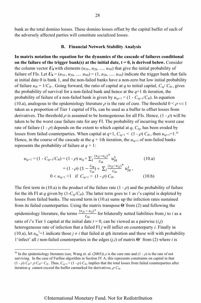
28

bank as the total domino losses. These domino losses offset by the capital buffer of each of the adversely affected parties will constitute socialized losses.

B. Financial Network Stability Analysis

In matrix notation the equation for the dynamics of the cascade of failures conditional on the failure of the trigger bank(s) at the initial date, t = 0, is derived below. Consider the column vector U0 with elements (u10 , u20, ..... uN0) that give the initial probability of failure of FIs. Let U0 = (u10 , u20, ..... uN0) = (1, u20, ..... uN0) indicate the trigger bank that fails at initial date 0 is bank 1, and the non-failed banks have a non-zero but low initial probability of failure ui0 = 1/Ci0 . Going forward, the ratio of capital at q to initial capital, Ciq/ Ci0 , gives the probability of survival for a non-failed bank and hence at the q+1 th iteration, the probability of failure of a non-failed bank is given by uiq+1 = (1 - Ciq+1/Ci0). In equation (10.a), analogous to the epidemiology literature is the rate of cure. The threshold 0 < taken as a proportion of Tier 1 capital of FIs, can be used as a buffer to offset losses from derivatives. The threshold is assumed to be homogeneous for all FIs. Hence, (1 - ) will be taken to be the worst case failure rate for any FI. The probability of incurring the worst case rate of failure (1 - ) depends on the extent to which capital at q, Ciq, has been eroded by losses from failed counterparties. When capital at q+1, Ciq+1 < (1 - ) Ci0 , then uiq+1=1. Hence, in the course of the cascade at the q + 1th iteration, the uiq+1 of non-failed banks represents the probability of failure at q + 1:

uiq+1 = (1 - Ciq+1/Ci0) = (1 - ) uiq + ∑ (10.a)

= (1 - 1 ∑

uiq+1 <1 if Ciq+1 > (1 - ) Ci0. (10.b) The first term in (10.a) is the product of the failure rate (1 - and the probability of failure for the ith FI at q given by (1-Ciq/Ci0). The latter term goes to 1 as i’s capital is depleted by losses from failed banks. The second term in (10.a) sums up the infection rates sustained from its failed counterparties. Using the matrix transpose ´from (2) and following the

epidemiology literature, the terms

for bilaterally netted liabilities from j to i as a

ratio of i’s Tier 1 capital at the initial date t = 0, can be viewed as a pairwise (i,j) heterogeneous rate of infection that a failed FI j will inflict on counterparty i. Finally in (10.a), let ujq

1=1 indicate those j i that failed at qth iteration and these will with probability 1‘infect’ all i non-failed counterparties in the edges (j,i) of matrix ´ from (2) where i is

30 In the epidemiology literature (see, Wang et. al. (2003)) is the cure rate and (1 - ) is the rate of not surviving. In the case of Furfine algorithm in Section IV A, this represents constraints on capital in that (1 - Ci0+ Ci0= Ci0 . Thus, Ciq+1 < (1 - Ci0, implies that the total losses from failed counterparties after iteration q cannot exceed the buffer earmarked for derivatives, Ci0.


29

exposed to j and there is zero impact between failed entities themselves (j,j). Non-failed banks, j, at q have zero impact on others j i and satisfy (10.a) if they survive to q + 1. FIs that fail prior to q - s, s >1, have zero impact on both themselves and others. This is an important ingredient as it represents the fact that once super-spreaders have demised, the contagion may halt as the network loses connectivity. Thus, in the algorithm depicting the contagion dynamics, Uq +1 is a non-negative vector that gives the incremental failure of banks at q + 1 (viz. banks that have not failed previously) where an indicator function F(z) sets row uiq+1 in the vector Uq +1 to equal uiq+1

1=1 to denote the failure of bank i, uiq+1 in (10 a,b) if i survives and uiq+1

0 = 0 if the FI had failed at or before q. Thus, for q>1 uiq+1 = F(zqF(zq) = uiq+1

1 = 1 if zq > 1,F(zq) = uiq+1 if 0 <zq < F(zq) = uiq+10 =0 (11.a)

with zq =(1 - uiq + ∑ q>1 (11.b)

and zq = 0 for all uiq-s

1, s 1, viz. i failed on or before q. (11.c) At q=1, as the initial probability of failure, ui0, of the non-trigger banks is assumed to be negligible at 1/Ci0, F(z1) = ui1 if 0 <z1 <and F(z1) = ui1

1 = 1, if

z1 = (1 - / Ci0 + ∑ + > . (11.d)

In contrast, in order to implement the eigen-pair stability analysis, as will be seen below, the linear characterization of the dynamical system in (10) and (11a-d) will overstate the damage caused by non-failed and failed banks as they will continue to ‘infect’ beyond their initial point of failure unlike the criterion in (11.c).31 The non-negative vector Uq +1 can be viewed as a metric of the damage rather than strict probability of failure at each q and the related stability conditions will limit a rampant uncontrolled growth of Uq as opposed to one that converges to a steady state. In other words, if the linear system satisfies stability conditions without the operation of the indicator function in (11 a-c), then the stability conditions will be satisfied in the presence of (11 a-c). Element for element, (11 a-c) produce smaller values than the vector Uq +1. The eigen-pair systemic risk analysis will be given in the following results.

31 In general, in the unconstrained case, in equation (10.a), uiq+1 = (1 - ) uiq + ∑ . That is, the

indicator function that signifies only banks that fail at q no longer follows and now we have a weighted

sum of the impact of all banks, j i in the second term.


30

Result 1: Matrix representation of financial network system

In order for the eigen-pair stability analysis to be used, in matrix notation the dynamics of financial contagion takes the following form:

Uq +1 = [(1 - + ´]Uq = QUq . (12)

Here, ´ is the transpose of the matrix in (2) with each element ij´= ji and I is the identity matrix. Recall that the elements of the 2nd row of ´, for example, take the following form: positive entries for counterparties 1, 3, …, N and with 0 to indicate that an FI does not ‘infect’ itself:

2´ =

… .

. (13)

Thus, for example with trigger bank that fails at the initial date being bank 1, from (10.a) and

(11.d) and noting that u20 = 1/ C20 , bank 2 will fail at the first iteration q = 1 if

>

Bank i effectively fails at q>1 from (11.b) when the sum of the rates of infection from others plus its own failure rate (1- uiq exceeds 1 (see footnote 28 for the constraint this places on losses from ‘infection’ at penultimate q before failure). The total number of failed FIs at q given by the contagion algorithm is:

N#q = q i uiq

1. (14) For some finite q, N#

q = N, i.e., the whole population can be wiped out. Result 2: Stability condition for financial network in (12)

The steady state of system (12) denoted by #is defined as one where #is a non-negative vector with some ui# <1 , viz if some nodes are to survive a local initial perturbation in the form of node failure. The system stability of (12) will be evaluated on the basis of the power iteration of the initial matrix Q=[(1 - + ´]. From (12), Uq takes the form:

Uq= [(1-)I´]qU0 = Qq U0. (15)

It can be shown that the stability of the system is governed by the maximum eigenvalue of the initial matrix Q = [(1 - ´ ] when it satisfies the condition:

max (Q) < 1 . 16) Expressing the eigenvalue equation in matrix notation, the qth power of matrix Q in (15) is: Q V = DV Q qV = DqV . (17)


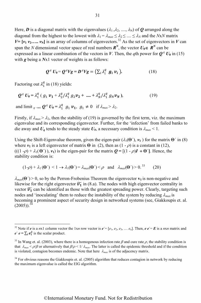
31

Here, D is a diagonal matrix with the eigenvalues (1 ,2, ...., N) of Q arranged along the diagonal from the highest to the lowest with 1 = max ≤ 2 ≤ .... ≤ N and the NxN matrix V= [v1 v2….. vN] is an array of columns of eigenvectors.32 As the set of eigenvectors in V can span the N dimensional vector space of real numbers RN, the vector U0 RN can be expressed as a linear combination of the vectors in V. Then, the qth power for Q q U0 in (15) with g being a Nx1 vector of weights is as follows: Q q U0 = Q qVg = D qVg ∑ . (18) Factoring out in (18) yields: Q q U0 = ( + / + .... + / ), (19) and limit q ∞ Q q U0 = , 0 if max > 2. Firstly, if max > 2, then the stability of (19) is governed by the first term, viz. the maximum eigenvalue and its corresponding eigenvector. Further, for the ‘infection’ from failed banks to die away and Uq tends to the steady state U#, a necessary condition is max < 1. Using the Shift-Eigenvalue theorem, given the eigen-pair (1(´), v1 ) for the matrix ´ in (8) where v1 is a left eigenvector of matrix in (2), then as (1 - ) is a constant in (12), (((1 -) + 1( ´) ), v1) is the eigen-pair for the matrix Q = [(1 - )I´]. Hence, the stability condition is: (1-) + 1 (´) < 1 1(´) = max(´) < and max(´) > 0.max(´) > 0, so by the Perron-Frobenius Theorem the eigenvector v1 is non-negative and likewise for the right eigenvector in (8.a). The nodes with high eigenvector centrality in vector can be identified as those with the greatest spreading power. Clearly, targeting such nodes and ‘inoculating’ them to reduce the instability of the system by reducing max is becoming a prominent aspect of security design in networked systems (see, Giakkoupis et. al. (2005)).34

32 Note if e is a nx1 column vector the 1xn row vector is e´= [e1, e2, e3, … en]. Then, e e´= E is a nxn matrix and e´ e = ∑ is the scalar product.

33 In Wang et. al. (2003), where there is a homogenous infection rate and cure rate , the stability condition is that max < / or alternatively that / < 1/max. The latter is called the epidemic threshold and if the condition is violated, contagion becomes endemic. Note that here max is of the adjacency matrix.

34 For obvious reasons the Giakkoupis et. al. (2005) algorithm that reduces contagion in network by reducing the maximum eigenvalue is called the EIG algorithm.


32

Result 3: Eigen-Pair analysis and role of maximum row sums

In the management of contagion and the design of the super-spreader tax or inoculation measures, it is important to understand the relationship between the maximum eigenvalue of and its corresponding eigenvectors and v1. In what follows, the role of row sums in the stability of the system ´ will be exploited. Firstly, it should be noted that the upper bound of the maximum eigenvalue max(´) is given by maximum of row sums of the matrix ´: max ≤ || ´||∞ = ∑ = maxi Si. (21) Here, || . ||∞ stands for the infinity norm of a matrix, which is the maximum of row sums Si where Si = ∑ . Hence, high connectivity to large number of counterparties and also large

exposures relative to capital contribute to the high row sum values for FIs and the largest of these constitutes the upper bound of max. Further, from the von Mises power iteration algorithm, Ralston (1965), which simultaneously generates the dominant eigenvalue of ´and its associated eigenvector, v1, the role of the scalar upper bound of || ´||∞ can be seen as follows. Starting with an initial column vector b0 of 1’s, the power iteration algorithm for the matrix ´ that yields the eigen-pair (max ,v1) is given by:

bq+1 =

|| || =

|| || . (22)

Here every element of the vector ´q+1b0 is normalized by its own maximum row sum resulting in the highest eigenvector central element to be 1. The iteration is said to have converged at q+1 when ´v1 = bq+1 = bq with an epsilon margin of error. This results in the eigenvalue equation in (8.b) ´v1 = λmax v1 . Clearly, at q+1, the scalar ||´q+1b0||∞ = max while ||´b0||∞ = || ´||∞ = maxi Si. Normalizing by the maximum row sum in (22) shows the direct relationship between Si = ∑ and max as given in the result in (21). However, for purposes

of designing the super-spreader tax, normalizing the numerator in (22) by the Euclidean norm ||´bq||2 will be followed so that the scalar product v1´v1=∑ =1. Note that the method of normalizing does not alter the converged values for the max of a matrix while the corresponding eigenvectors using the two methods differ by a constant multiplicative factor.35 Finally, the power iteration algorithm in (22) delivers the two ingredients needed to design systemic risk measures and mitigants for an interconnected system in terms of the eigen-pair max and the associated centrality measures of the individual FIs.

35 Here, denote the eigenvector obtained by the norm ||.||∞ as v1||.||∞ and the one by the norm ||.||2 simply as v1. Let g be a constant and g v1||.||∞ = v1. Then g2 v1||.||∞ v1||.||∞ = v1 v1 = 1. This gives g = (1/ v1||.||∞ v1||.||∞ )1/2. Note that v1||.||∞ v1||.||∞ is simply the sum of squares of the elements of the vector v1||.||∞ .


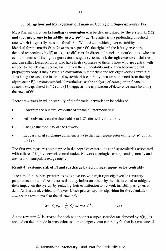
33

C. Mitigation and Management of Financial Contagion: Super-spreader Tax

Most financial networks leading to contagion can be characterized by the system in (12) and they are prone to instability at max(´) > The latter is the prefunding threshold rate, which is typically the same for all FIs. While max—which governs stability— is identical for the matrix in (2) or its transpose ´, the right and the left eigenvectors, denoted respectively by and v1, are different. In directed financial networks, those who are central in terms of the right eigenvector instigate systemic risk through excessive liabilities and can inflict losses on those who have high exposures to them. Those who are central with respect to the left eigenvector, viz. high on the vulnerability index, then become potent propagators only if they have high correlation in their right and left eigenvector centralities. This being the case, the individual systemic risk centrality measures obtained from the right eigenvector is recommended. Nevertheless, as the analysis of contagion in financial systems encapsulated in (12) and (15) suggests, the application of deterrence must be along the rows of ´. There are 4 ways in which stability of the financial network can be achieved: Constrain the bilateral exposure of financial intermediaries;

Ad-hocly increase the threshold in (12) identically for all FIs;

Change the topology of the network;

Levy a capital surcharge commensurate to the right eigenvector centrality of a FI in (12).

The first two measures do not price in the negative externalities and systemic risk associated with failure of highly network central nodes. Network topologies emerge endogenously and are hard to manipulate exogenously.

Result 4: Systemic risk of FI and surcharge based on right eigen-vector centrality

The aim of the super-spreader tax is to have FIs with high right eigenvector centrality parameters to internalize the costs that they inflict on others by their failure and to mitigate their impact on the system by reducing their contribution to network instability as given by max. As discussed, critical to the von-Mises power iteration algorithm for the calculation of λmax are the row sums Si of the ith row in ´:

Si = ∑ ∑ . (23)

A new row sum Si

# is created for each node so that a super-spreader tax denoted by is applied on the ith node in proportion to its right eigenvector centrality that is a measure of


34

its systemic risk:36

Si# = ∑ # ∑ . (24)

The rationale behind this application of the right eigenvector centrality of a node as the basis of the super-spreader tax is to enable a node to provide a buffer proportional to its own capacity to propagate contagion. Note that the funds that will be escrowed here using is not calibrated to mitigate failure of FI i due to its exposures to j counterparties, but it is in keeping with its own spreading powers. Thus, Si

# < Si for > 0. (25) We will consider two formulations of the super-spreader tax: = , 0 < ≤ 1 or >1, (26.a) and = , 0 < ≤ 1 or >1. (26.b) In (26.a), the super-spreader tax is a linear function of a FI’s eigenvector centrality while the super-spreader tax is set proportionate to rather than to in (26.b). The advantage of this is that is a naturally normalized variable with ∑ 1. Further, with the super-spreader tax being a function of rather than , this will penalize nodes with higher eigenvector centrality more than others. This is useful when the dominant eigenvector central node is distinctly more dominant than others and hence the progressivity of the tax rate becomes more apparent with the application of than of . In contrast, when several nodes are equally dominant, the use of = is more appropriate. Finally, as 0 ≤ < 1, equation (26.a) can extract more tax across the population with non-zero centrality measures than a tax rate using and hence also deliver faster rates of decline of the max of the system.

36 Clearly, it is possible to apply the capital surcharge in denominator of (23),

Si# = ∑ # ∑ . This was, in fact, tried out in an earlier draft of the paper. But

following the principle of ‘greedy’ algorithms as in the EIG algorithm of Giakkoupis et. al. (2005) that seek the largest possible reductions of the maximum eigenvalue of the system, the current proposal in (24) was found to be more effective. Note, the algorithm applied in equation (24) was constrained to retain a non-negative matrix for ´#().


35

The network stabilization algorithm will be called the EIG algorithm in keeping with Giakkoupis et. al. (2005). The new matrix associated with Si

#() will be denoted as ´#(). The alpha parameter when set at 0 obtains the max associated with the untaxed initial matrix ´. When =1, each node is exactly penalized by or that yields the max for ´#(). Considering, 1> , there is a monotonic reduction in the max associated with the matrices {´#()} corresponding to the monotonic reduction in row sums Si

#(1) < Si#(= 1) < ...

< Si#(= 0.75)<... < Si

#(= 0.5) < ...< Si(=0). The case of 1 may apply when the initial matrix ´ needs a more aggressive application of the tax to stabilize the matrix to the point where Si

#(1) for all i such that max< for ´#(). Clearly, if > 1 is needed to stabilize the system, the sustainability of such a market for risk sharing is in question. In fact, full stabilization to levels of max(´#) may not be technically possible and/or economically feasible. However, what the eigen-pair method of estimating and managing systemic risk in an interconnected financial network based on bilateral on- and off-balance sheet data provides is a clear cut mathematical benchmark for whether the system has become more or less unstable and who within it contributes most to this. The nature of the systemic risk stabilization super-spreader fund is that it operates like an escrow fund. The funds commensurate to each FI’s surcharge as a proportion to their Tier 1 capital are collected at some initial point whether within a centralized clearing platform (CCP) context or by the regulatory authority. The funds are deployed at the time of the failure of a FI for the collective good. The funds escrowed from the failing FI will contribute according to its right eigenvector centrality to restore to the others the domino losses delineated in the Furfine algorithm of Section IV.A. Note that the tax collected from non-failed banks with high eigenvector centrality will also have to be used during a financial contagion. The degree of stabilization being sought can be calibrated. A full stabilization of matrix ´ to achieve max< may be not be necessary and may be prohibitively expensive. Note that the function of the super-spreader tax escrow fund is not to collect the loss of capital for the system as a whole at the end point q# of the Furfine contagion algorithm. Rather it is a measure of the under capitalization or collateralization relative to what is needed for network stability. Finally, the systemic risk super-spreader fund can be designed to work in a clustered hierarchical network where contagion takes a specific pathway amongst the central tier if a highly connected node fails. This lite super-spreader tax fund aims to cover the losses that the most connected nodes will inflict on their direct ‘big’ neighbors in the first tier, q = 1. The empirical section will demonstrate these points quantitatively.

V. EMPIRICAL RESULTS: NETWORK ANALYSIS OF THE CALIBRATED AGGREGATED

GLOBAL DERIVATIVES MARKET

Here I start with the construction of the network of bilateral financial obligations based on firm level data aggregated over all derivatives products and all over counterparties. The sample data for 2009:Q4 for the top 22 FIs of the 202 market participants is reported in


36

Appendix Table A.1. The variables reported there is for derivatives gross notional, gross positive fair value, gross negative fair value, derivatives assets, derivatives liabilities and Tier 1 capital. As discussed in Section III.D, the network algorithm works on the basis of the Zhou and Mondragon (2003) modified preferential attachment principle in order to achieve the sparse adjacency matrix and the core-periphery network structure so as to reflect empirical observations on the high level of concentration of exposures among the top 12 derivatives broker dealers (see footnote 16). A further constraint that is met is that the bilaterally netted matrix crucial for the stability and contagion analysis, described in Section IV, satisfies the empirical data for each FI in regard to their derivatives assets and derivatives liabilities. We design a ‘shuffle algorithm’ for the bilateral netted M matrix described in Section II.B so that the errors are brought to about 2 percent of the actual data for the M matrix on average.

A. Empirical (Small World) Core-Periphery Network Algorithm

The adjacency matrix for X in (1) is constructed from the empirically based market shares in the relevant market data given in Appendix Table A.1. Our algorithm assigns out degrees for a FI in terms of its respective market share in terms of the GNFV of derivatives. Due to the regional aspect of the global derivatives market, there is some regional clustering in FI’s allocation of out-degrees. Denoting: : market share of derivatives gross notional

: Gross Negative Fair Value for which is a guarantor vis-à-vis its counterparties : Gross Positive Fair Value for which is beneficiary vis-à-vis its counterparties

The algorithm allocates to each of row bank i’s counterparties j, a value of its GNFV equal to

and if j

iij GGS , then bank i allocates the remaining to the external non-U.S. and

European financial entities which are collectively denoted as the N+1 agent. The column sums of matrix X in (1) are made to satisfy the GPFVj or Bj for each bank, and if

ji

ij BGS , the remaining is bought from the external N+1entity. The gross flow X

matrix so constructed using the above algorithm is a sparse matrix with a very high concentration of activity in the top left hand side of the matrix. The bilaterally netted matrix

M of Section II.B is constructed to satisfy the condition that, mij > 0, j

jiij xx )( will equal

the data determined derivatives liabilities for the FIs up to some (2 percent) average margin

of error.37 Likewise, the sum of the negative entries, mij < 0, j

jiij xx )( for each FI i in the

37 Using the gross bilateral X matrix constructed as above as the initial matrix, Rais Shaghaghi and Markose (2012) apply a genetic algorithm to implement the empirical constraints on the netted bilateral flows between counterparties. As there are multi-objectives regarding minimization of errors from a number of different

(continued…)


37

ith row gives its bilaterally netted receivables for all derivatives products, which as explained above is calibrated to satisfy the data determined derivatives assets for that FI. The network for the bilaterally netted matrix is plotted below. In Figure 4, the red nodes denote those with derivatives liabilities in excess of 6 percent market share or are solely derivatives sellers and blue nodes are the remaining. JP Morgan and Bank of America occupy central status with 2 tiers of FIs around them. Over 80 percent of the banks are in the periphery with almost no connectivity among themselves reflecting a very sparse adjacency matrix.

Figure 4. Empirically Constructed Global Derivatives Network (Bilaterally Netted) Aggregated over all Derivatives Products for FIs and Outside Entities

(Triangle): Empirical Small World Network in Tiered Layout

Source: Constructed by author from bilaterally netted derivatives data (2009 Q4)for 204 FISs.

constraints, some 100,000 generations of the genetic algorithm were needed to produce M+ matrices with errors which were less than 2 percent on average from the empirical data on derivatives liabilities and assets. Of these, the M+ matrices from top 8 runs were selected. As the unweighted matrix is identical, the sparseness and core-periphery structure does not change in all the runs and likewise the TITF property in the Furfine contagion. The M+ matrix analyzed in this paper has a 20 percent standard deviation in the ‘fitted’ derivatives liabilities, biased in the direction of the more eigen-vector central FIs.


38

The tiered layout in Figure 4 is constructed in the following way. First the full range of connectivity of all banks is taken in terms of the ratio of each bank’s total in and out degrees divided by total number of connected links of the most connected FI. FIs that are a ranked in the top 10 percentile of this ratio constitute the inner core. This is followed by a mid core between 90 and 70 percentile and a 3rd tier between 40 and 70 percentile. Those with connectivity ratio less than 40 percentile are categorized as the periphery. The tiering algorithm that produced Figure 4 has the constraint that those in the periphery are not connected to one another. The triangles in Figure 4 represent non-bank FIs and non-U.S. and European FIs.

B. Global Derivatives Network Statistics (2009:Q4)

As with any complex network it is important to understand the topology and structure of the network in terms of the network statistics based on the degree distribution. Table 3 gives the network statistics for the empirically constructed global derivatives networks for the case for 202 nodes which involve banks only and 204 nodes where the last two nodes include non-bank FIs and the external balancing node representing banks outside of U.S. and Europe. As we do not have explicit data on these, they are modeled not to fail in the contagion experiments. Network statistics are reported for both these cases. Table 3 indicates the sparseness of the network which can be seen from the average number of in and out degrees of about 2.3 and low connectivity of only 1 percent. With no isolated subgraphs for the network, such a low level of connectivity manifests the very high efficiency of link formation. The distribution of out degrees from FIs shows greater asymmetry than does that of in degrees in terms of all higher moments given by standard deviation, skewness and kurtosis. Three statistics for the empirical highly tiered derivatives network stand out in contrast to an equivalent random graph. Firstly, the cluster coefficient is about 0.48 whereas that for an Erdös-Renyi random graph this will be closer to the connectivity for the network of 0.01. Also, random graphs have substantially low variance to mean ratios, <k2>/<k>, of less than 1 when compared to that of the empirically calibrated network for derivatives exposures of FIs. Table 3 shows the latter to be in excess of 7.


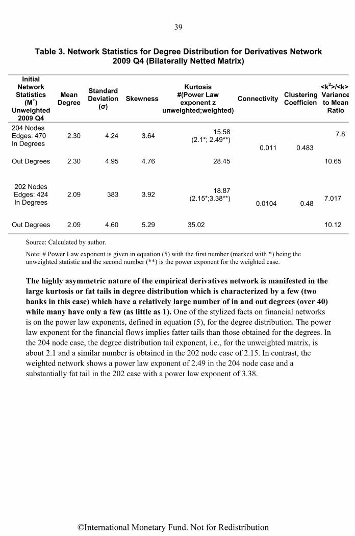
39

Table 3. Network Statistics for Degree Distribution for Derivatives Network 2009 Q4 (Bilaterally Netted Matrix)

Initial

Network Statistics

(M+) Unweighted

2009 Q4

Mean Degree

Standard Deviation

(σ) Skewness

Kurtosis #(Power Law exponent z

unweighted;weighted)

Connectivity ClusteringCoefficient

<k2>/<k>Varianceto Mean

Ratio

204 Nodes Edges: 470 In Degrees

2.30 4.24 3.6415.58

(2.1*; 2.49**)0.011 0.483

7.8

Out Degrees 2.30 4.95 4.76 28.45 10.65

202 Nodes Edges: 424 In Degrees

2.09 383 3.9218.87

(2.15*;3.38**)0.0104 0.48

7.017

Out Degrees 2.09 4.60 5.29 35.02 10.12

Source: Calculated by author.

Note: # Power Law exponent is given in equation (5) with the first number (marked with *) being the unweighted statistic and the second number (**) is the power exponent for the weighted case. The highly asymmetric nature of the empirical derivatives network is manifested in the large kurtosis or fat tails in degree distribution which is characterized by a few (two banks in this case) which have a relatively large number of in and out degrees (over 40) while many have only a few (as little as 1). One of the stylized facts on financial networks is on the power law exponents, defined in equation (5), for the degree distribution. The power law exponent for the financial flows implies fatter tails than those obtained for the degrees. In the 204 node case, the degree distribution tail exponent, i.e., for the unweighted matrix, is about 2.1 and a similar number is obtained in the 202 node case of 2.15. In contrast, the weighted network shows a power law exponent of 2.49 in the 204 node case and a substantially fat tail in the 202 case with a power law exponent of 3.38.


40

Table 4. Rich Club Statistics (See, Equation (6))

VI. Out

VII. Degree

VIII. (k)

IX. Rich Club

X. Coefficient

XI. Number of

XII. Nodes N(kd))

Selected Members

k > 0 0.03 150 k > 1 0.22 42 k > 2 0.38 30 k > 3 0.64 21 Standard Charter k > 4 0.67 20 k > 6 0.69 19 Societe Generale k > 7 0.71 18 Dexia, Uni-Credit

k > 8 0.91 13

New York Mellon, UBS,HSBC

k > 9 0.95 11

Credit Suisse, Credit Agricole,

k > 10 1 9

Barclays, BNP Paribas, RBS

k > 12 1 6 Morgan Stanley

k > 13 1 4

Deutsche Bank, Citigroup

k > 16 1 3 Goldman Sachs k > 17 1 2 Bank of America k > 30 1 1 JPMorgan


Membership of the rich club given in equation (6) with (k) = 1 is determined using out degrees, ki. Note the number of FIs with ki > 0 is only 150 out of a total of 202 nodes. As Table 4 shows there are 4 distinct groupings of rich club statistics. The members included in the rich club statistic from (k) = 1 to (k) = 0.91, are those who are part of an almost complete central cluster. These include 14 major broker-dealers. In the next section, it will be shown that threats can arise from those FIs that occupy the second set of rich club coefficients in the range {0.71 0.69} and also from a couple in the range {0.64, 0.69}. Recall, even though members with low rich club coefficients have fewer out degrees, those that connect to the inner core of the network will have high eigenvector centrality and hence the capacity to trigger contagion. The 100 or so FIs on the periphery have a rich club coefficient of 0.03.

C. Eigenvector Centrality and Furfine Stress Test Results

Here I will empirically examine the role of ‘super-spreaders’ of contagion in the derivatives markets in terms of their network connectivity and their eigenvector centrality. The results of the Furfine contagion stress tests described in Section IV A are also given. Table 5 indicates that there is considerable difference in the ranking of FIs in respect


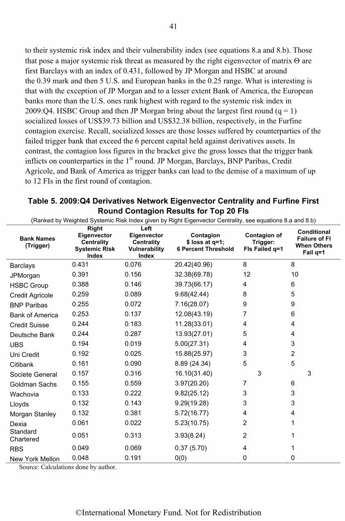
41

to their systemic risk index and their vulnerability index (see equations 8.a and 8.b). Those that pose a major systemic risk threat as measured by the right eigenvector of matrix are first Barclays with an index of 0.431, followed by JP Morgan and HSBC at around the 0.39 mark and then 5 U.S. and European banks in the 0.25 range. What is interesting is that with the exception of JP Morgan and to a lesser extent Bank of America, the European banks more than the U.S. ones rank highest with regard to the systemic risk index in 2009:Q4. HSBC Group and then JP Morgan bring about the largest first round (q = 1) socialized losses of US$39.73 billion and US$32.38 billion, respectively, in the Furfine contagion exercise. Recall, socialized losses are those losses suffered by counterparties of the failed trigger bank that exceed the 6 percent capital held against derivatives assets. In contrast, the contagion loss figures in the bracket give the gross losses that the trigger bank inflicts on counterparties in the 1st round. JP Morgan, Barclays, BNP Paribas, Credit Agricole, and Bank of America as trigger banks can lead to the demise of a maximum of up to 12 FIs in the first round of contagion. Table 5. 2009:Q4 Derivatives Network Eigenvector Centrality and Furfine First

Round Contagion Results for Top 20 FIs (Ranked by Weighted Systemic Risk Index given by Right Eigenvector Centrality, see equations 8.a and 8.b)

Bank Names (Trigger)

Right Eigenvector Centrality

Systemic Risk Index

Left Eigenvector Centrality

Vulnerability Index

Contagion $ loss at q=1;

6 Percent Threshold

Contagion of Trigger:

FIs Failed q=1

Conditional Failure of FI When Others

Fail q=1

Barclays 0.431 0.076 20.42(40.96) 8 8

JPMorgan 0.391 0.156 32.38(69.78) 12 10

HSBC Group 0.388 0.146 39.73(66.17) 4 6

Credit Agricole 0.259 0.089 9.68(42.44) 8 5

BNP Paribas 0.255 0.072 7.16(28.07) 9 9

Bank of America 0.253 0.137 12.08(43.19) 7 6

Credit Suisse 0.244 0.183 11.28(33.01) 4 4

Deutsche Bank 0.244 0.287 13.93(27.01) 5 4

UBS 0.194 0.019 5.00(27.31) 4 3

Uni Credit 0.192 0.025 15.88(25.97) 3 2

Citibank 0.161 0.090 8.89 (24.34) 5 5

Societe General 0.157 0.316 16.10(31.40) 3 3

Goldman Sachs 0.155 0.559 3.97(20.20) 7 6

Wachovia 0.133 0.222 9.82(25.12) 3 3

Lloyds 0.132 0.143 9.29(19.28) 3 3

Morgan Stanley 0.132 0.381 5.72(16.77) 4 4

Dexia 0.061 0.022 5.23(10.75) 2 1 Standard Chartered

0.051 0.313 3.93(8.24) 2 1

RBS 0.049 0.069 0.37 (5.70) 4 1

New York Mellon 0.048 0.191 0(0) 0 0 Source: Calculations done by author.


42

In the exposure stakes measured by the vulnerability index, Goldman Sachs followed by Morgan Stanley rank the highest. Dexia, Unicredit, and Standard Charter are the least connected with less than 2 percent of total links. As shown in the last two columns of Table 5, in such densely clustered structures, there is high correlation between those who can inflict contagion directly on their counterparties and those who are directly vulnerable to the failure of others. Figures 5.a–5.f show the devastating consequences of ‘the too interconnected to fail’ (TITF) phenomenon. The empirically calibrated network of derivatives liabilities that has produced a highly clustered central core, results in a characteristic propagation of contagion. To date, this has not be sufficiently quantified or modeled in the case of financial networks. Note a 6 percent capital threshold has been assumed for the system dynamics in equation (12) with conditions (11a-d) in place. As can be seen in Figures 5.a–5.f, whether the trigger bank directly kills 12 in the first round of contagion in the case of JP Morgan, 7 in the case of Goldman Sachs, 4 in the case of UBS, or even only 2 in the case of Standard Charter, the contagion with no interventions can spread at great speed to the 3rd and 4th iteration (q = 3, q = 4 in the Furfine terminology given in Section IV.A and shown as concentric circles in Figure 5) of the tiered OTC derivatives market. This will bring down a similar number (25) of FIs and the potential total domino loss of Tier 1 capital from all of these cases as shown in Figures 5a–5f is approximately US$350 billion which is 25 percent of total Tier 1 capital of US$1.413 trillion for the 202 FIs given in Table 1. Clearly, the failure of JP Morgan will trigger the fastest self-annihilating contagion which ends at q = 2. This phenomenon where a clustered group of banks stand or fail together is what we called TITF. Even though the overall connectivity of the global derivatives network was low at 1 percent, the tiered structure with heavy concentration of exposures is what causes this outcome. There is also the feature that others endowed with fewer out degrees can provoke a slower growing contagion as in the case of Standard Charter with only 5 out degrees. Finally, while there is some regional bias in that the failure of UBS and Deutsche Bank will certainly affect other big regional FIs, the global implications of failure are immediately apparent in the plots of the Furfine contagion algorithm.


43

Figure 5. Furfine Contagion Stress Test on Empirical Calibrated Derivatives Network 2009:Q4 (203 FIs) 6 percent Capital Threshold

(Black nodes are failed banks; trigger bank in centre)

Figure 5aTrigger Bank JP Morgan: q=1 FIs Failed 12 Figure 5b Trigger bank Goldman Sachs: q=1 FIs failed 7 Total FIs failed 25; 24.48 % Tier 1 Capital Loss US$345.94bn Total FIs failed 25; 25 % Tier 1 Capital Loss US$355.75 bn

Figure 5c Trigger bank UBS: q=1 FIs Failed 4 Figure 5d Trigger bank Deutsche Bank: q =1 FIs failed 5 Total FIs failed 26; 24.67 % Tier 1 Capital Loss US$348.66bn Total FIs failed 25; 25 % Tier 1 Capital Loss US$355.75

Figure 5e Trigger Bank Credit Suisse: q=1 FIs failed 5 Figure 5f Trigger Bank Standard Chartered: q=1 FI Failed 1 Total FI Failed 25; 24.67 % Tier 1 Capital US$348.61 bn Total FI failed 25; 25 % Tier 1 Capital US$351.81 bn

Source: Plotted using author’s software.


44

D. Quantification and Evaluation of the Super-spreader Tax (2009 Q4)

At the maximum eigenvalue for the system in (12)max (Q) 1.57 (or max(= 0.57 which is greater than the capital threshold = 0.06), the derivatives market is deemed unstable and the losses to the system as a whole from the failure of any of top 20 eigenvector dominant banks, can be nothing short of catastrophic. The systemic risk is assessed solely on the basis of the matrix of the ratio of derivatives liabilities to Tier 1 capital with the contagion dynamics governed by the equation (12). The total loss of Tier 1 capital from contagion is in the order of about US$350 billion irrespective of which of the top FIs were to fail, with only the speed of contagion differing with different trigger banks. This is important to understand as the bulk of macro-prudential discussions focus on SIFIs rather than on unstable networks of financial liabilities. The objective of levying a derivatives market surcharge is that the socialized losses that arise from the interconnectivity of FIs have to be internalized by the FIs themselves. The question is, what is price of stability? Does the full amount of US$350 billion less the capital buffers on derivatives assets of the 25 or so adversely affected counterparties need to be escrowed via taxes to achieve full stabilization ? In this section, I will evaluate the super-spreader tax based on a theoretical derivation in Section IV.C and equations (26.a and 26.b). Note the eigenvector centrality for the top 20 banks for the initial untaxed system is given in Table 5. A surcharge on a FI’s capital commensurate to its right eigenvector centrality using the formulae in equation (26.a) = (or equation (26.b) = ) is applied to the rows of ´ for different values of 0 < ≤ 1. This results in a monotonic reduction in the maximum eigenvalue #

max associated with the matrices {´#()} corresponding to the monotonic reduction in row sums Si

#(=1) < .. < Si

#(=0.75)<... < Si#(= 0.5) < ...< Si(= 0). The results of the EIG-algorithm are

given in Figure 6. What is clear from Figure 6 is that the application of the super-spreader tax formula = in (26.a), rather than the one in (26.b), brings down the #

max of the system much faster for all values of . Secondly, at when the #

max (´) of the system comes close to = 0.03, which far exceeds the stability target, the maximum eigen-value power iteration algorithm ceased to converge. Clearly there are technical and economic limits to how much a given unstable system can be stabilized. The super-spreader tax rate for each FI, given in Table 6, is obtained by multiplying the right eigenvector centrality of each node by the alpha parameter given in equation

(26a). This is then evaluated against the #max (´) for the system and also in terms of how

much funds will accrue as shown in Table 7. To get the dollar value of the capital surcharge, the tax rates are multiplied by the Tier 1 capital of each FI. The last row of Table 7 shows the amounts the super-spreader escrow fund can obtain by using different tax rates on the 20 FIs with the highest systemic risk indices based on their right eigenvector centrality. Strictly speaking, the figures in the last row of Table 7 refers to the funds if deployed in keeping with


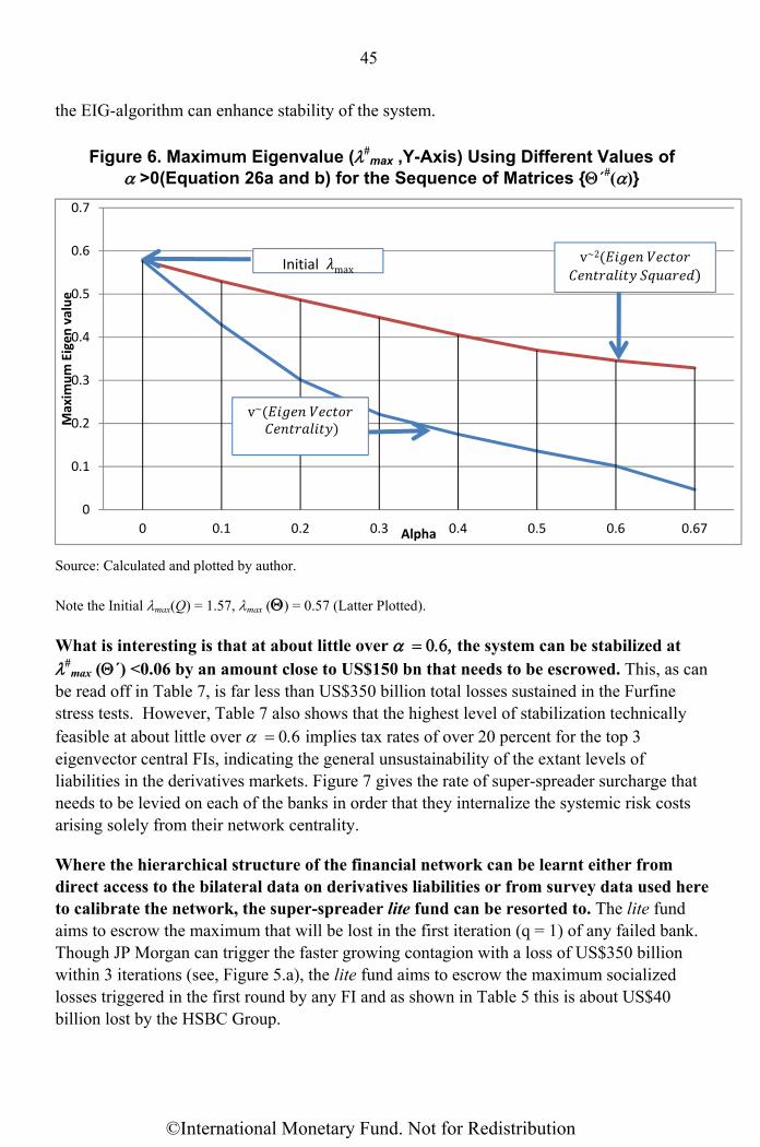
45

the EIG-algorithm can enhance stability of the system.

Figure 6. Maximum Eigenvalue (#max ,Y-Axis) Using Different Values of

>0(Equation 26a and b) for the Sequence of Matrices {´#()}

Source: Calculated and plotted by author.

Note the Initial max(Q) = 1.57, max () = 0.57 (Latter Plotted).

What is interesting is that at about little over the system can be stabilized at #

max (´) <0.06 by an amount close to US$150 bn that needs to be escrowed. This, as can be read off in Table 7, is far less than US$350 billion total losses sustained in the Furfine stress tests. However, Table 7 also shows that the highest level of stabilization technically feasible at about little over implies tax rates of over 20 percent for the top 3 eigenvector central FIs, indicating the general unsustainability of the extant levels of liabilities in the derivatives markets. Figure 7 gives the rate of super-spreader surcharge that needs to be levied on each of the banks in order that they internalize the systemic risk costs arising solely from their network centrality.

Where the hierarchical structure of the financial network can be learnt either from direct access to the bilateral data on derivatives liabilities or from survey data used here to calibrate the network, the super-spreader lite fund can be resorted to. The lite fund aims to escrow the maximum that will be lost in the first iteration (q = 1) of any failed bank. Though JP Morgan can trigger the faster growing contagion with a loss of US$350 billion within 3 iterations (see, Figure 5.a), the lite fund aims to escrow the maximum socialized losses triggered in the first round by any FI and as shown in Table 5 this is about US$40 billion lost by the HSBC Group.

0

0.1

0.2

0.3

0.4

0.5

0.6

0.7

0 0.1 0.2 0.3 0.4 0.5 0.6 0.67

Max

imu

m E

ige

n v

alu

e

Alpha

v~

v~2Initial max


46

Figure 7. Individual FI Tax Rates Obtained by Multiplying Right Eigenvector Centrality by Different Values of Alpha > 0 (Using Equation 26a)


The lite super-spreader fund option that secures enough liquidity to buffer first tier losses which is a relatively small sum of US$40bn implies tax rates of 8–9 percent for the 3 FIs with the highest systemic risk index, followed by 5 FIs taxed at 5 percent , 3 at 2.5 percent and the remaining at 1 percent or so. This is marked in Figure 7 and highlighted in Table 7.

0

0.05

0.1

0.15

0.2

0.25

0.3

0 0.1 0.2 0.3 0.4 0.5 0.6

Tax

Rat

e %

alpha

Barclays

JPMorgan

HSBC

Credit Agricole

BNP Paribas

BoA

Credit Suisse

Deutsche Bank

UBS

Uni Credit

Citibank

Societe General

Goldman Sachs

Wachovia

Lloyds

Morgan Stanley

Dexia

Standard Chartered

Lite super-spreader tax fund based on top 20 FIs' eigenvector centrality (V) can cover largest 1st round losses


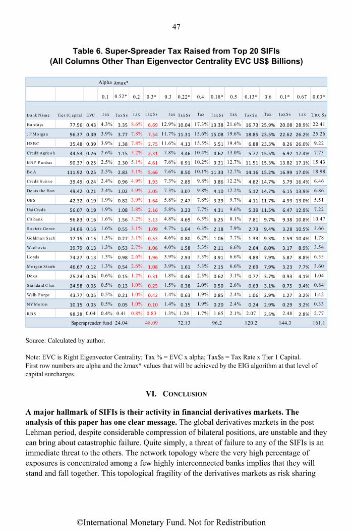
47

Table 6. Super-Spreader Tax Raised from Top 20 SIFIs (All Columns Other Than Eigenvector Centrality EVC US$ Billions)


Note: EVC is Right Eigenvector Centrality; Tax % = EVC x alpha; Tax$s = Tax Rate x Tier 1 Capital. First row numbers are alpha and the λmax* values that will be achieved by the EIG algorithm at that level of capital surcharges.

VI. CONCLUSION

A major hallmark of SIFIs is their activity in financial derivatives markets. The analysis of this paper has one clear message. The global derivatives markets in the post Lehman period, despite considerable compression of bilateral positions, are unstable and they can bring about catastrophic failure. Quite simply, a threat of failure to any of the SIFIs is an immediate threat to the others. The network topology where the very high percentage of exposures is concentrated among a few highly interconnected banks implies that they will stand and fall together. This topological fragility of the derivatives markets as risk sharing

Alpha λmax*

0.1 0.52* 0.2 0.3* 0.3 0.22* 0.4 0.18* 0.5 0.13* 0.6 0.1* 0.67 0.03*

Bank Name Tier 1 Capita l EVC Tax Tax $ s

Tax

Tax $ s Tax Tax $ s Tax Tax $ s Tax Tax $ s

Tax Tax $ s Tax Tax $s

Barclays 77.56 0.43 4.3% 3.35 8.6% 6.69 12.9% 10.04 17.3% 13.38 21.6% 16.73 25.9% 20.08 28.9% 22.41

J P Mo rgan 96.37 0.39 3.9% 3.77 7.8% 7.54 11.7% 11.31 15.6% 15.08 19.6% 18.85 23.5% 22.62 26.2% 25.26

HSBC 35.48 0.39 3.9% 1.38 7.8% 2.75 11.6% 4.13 15.5% 5.51 19.4% 6.88 23.3% 8.26 26.0% 9.22

Credit Agrico le 44.53 0.26 2.6% 1.15 5.2% 2.31 7.8% 3.46 10.4% 4.62 13.0% 5.77 15.5% 6.92 17.4% 7.73

BNP P aribas 90.37 0.25 2.5% 2.30 5.1% 4.61 7.6% 6.91 10.2% 9.21 12.7% 11.51 15.3% 13.82 17.1% 15.43

Bo A 111.92 0.25 2.5% 2.83 5.1% 5.66 7.6% 8.50 10.1% 11.33 12.7% 14.16 15.2% 16.99 17.0% 18.98

Credit Suis s e 39.49 0.24 2.4% 0.96 4.9% 1.93 7.3% 2.89 9.8% 3.86 12.2% 4.82 14.7% 5.79 16.4% 6.46

Deuts che Bank 49.42 0.21 2.4% 1.02 4.9% 2.05 7.3% 3.07 9.8% 4.10 12.2% 5.12 14.7% 6.15 13.9% 6.86

UBS 42.32 0.19 1.9% 0.82 3.9% 1.64 5.8% 2.47 7.8% 3.29 9.7% 4.11 11.7% 4.93 13.0% 5.51

Uni Credit 56.07 0.19 1.9% 1.08 3.8% 2.16 5.8% 3.23 7.7% 4.31 9.6% 5.39 11.5% 6.47 12.9% 7.22

Citibank 96.83 0.16 1.6% 1.56 3.2% 3.13 4.8% 4.69 6.5% 6.25 8.1% 7.81 9.7% 9.38 10.8% 10.47

So cie te Genera 34.69 0.16 1.6% 0.55 3.1% 1.09 4.7% 1.64 6.3% 2.18 7.9% 2.73 9.4% 3.28 10.5% 3.66

Go ldman Sach 17.15 0.15 1.5% 0.27 3.1% 0.53 4.6% 0.80 6.2% 1.06 7.7% 1.33 9.3% 1.59 10.4% 1.78

Wacho via 39.79 0.13 1.3% 0.53 2.7% 1.06 4.0% 1.58 5.3% 2.11 6.6% 2.64 8.0% 3.17 8.9% 3.54

Llo yds 74.27 0.13 1.3% 0.98 2.6% 1.96 3.9% 2.93 5.3% 3.91 6.6% 4.89 7.9% 5.87 8.8% 6.55

Mo rgan S tanle 46.67 0.12 1.3% 0.54 2.6% 1.08 3.9% 1.61 5.3% 2.15 6.6% 2.69 7.9% 3.23 7.7% 3.60

Dexia 25.24 0.06 0.6% 0.15 1.2% 0.31 1.8% 0.46 2.5% 0.62 3.1% 0.77 3.7% 0.93 4.1% 1.04

Standard Chart 24.58 0.05 0.5% 0.13 1.0% 0.25 1.5% 0.38 2.0% 0.50 2.6% 0.63 3.1% 0.75 3.4% 0.84

Wells Fargo 43.77 0.05 0.5% 0.21 1.0% 0.42 1.4% 0.63 1.9% 0.85 2.4% 1.06 2.9% 1.27 3.2% 1.42

NY Mello n 10.15 0.05 0.5% 0.05 1.0% 0.10 1.4% 0.15 1.9% 0.20 2.4% 0.24 2.9% 0.29 3.2% 0.33

RBS 98.28 0.04 0.4% 0.41 0.8% 0.83 1.3% 1.24 1.7% 1.65 2.1% 2.07 2.5% 2.48 2.8% 2.77

Superspreader fund 24.04 48.09 72.13 96.2 120.2 144.3 161.1


48

institutions has an implicit moral hazard problem that undermines their social usefulness. The empirically calibrated network for derivatives liabilities manifests a highly clustered core-periphery structure and extreme form of TITF as seen in Figures 5.a- 5.f. The implied socialized losses are very large (to the tune of US$350 billion) and the liabilities arising from extant derivatives network structures cannot be supported by the existing capital base.38 The good news is that the highly clustered network structure permits targeted management of systemic risk. One of the main contributions of the paper is to use network analysis to design a set of surcharges that will enable the SIFIs in the derivatives markets to internalize the costs imposed on other FIs and also the tax payer by their failure. This paper is among the first to show how network stability, which is based on the maximum eigenvalue of a non-positive financial matrix of liabilities, relates to the right eigenvector centrality of FIs and their contagion spreading capabilities in the system. The right eigenvector centrality has been identified as providing the systemic risk index for each FI while the left eigenvector centrality yields the exposure or vulnerability index of FI. A progressive capital surcharge rate based on the right eigenvector centrality of each FI in the pre-tax setting is designed and calibrated in Section V.D in order to achieve a much more stable system with a reduced maximum eigenvalue. As in the case of the 2009:Q4 derivatives liabilities data, while an escrowed amount of about US$150 billion as shown in Table 7 can technically stabilize the system, it implies tax rates of over 20 percent on the super-spreaders. The hierarchical core-periphery structure of networks of liabilities in off-balance sheet financial interactions, enables the design of a super-spreader lite escrow account based on the surcharges on 20 FIs with non-negligible right eigenvector centrality. The objective of the lite fund is to be able to cover the maximum direct first round losses that could be inflicted by a failed FI, which is estimated to about US$40 billion. Operationalizing macro-prudential policy is now well understood to revolve around the following. First, how to measure systemic risk of a financial system is an important aspect in operationalizing macro-prudential policies. While a whole array of systemic risk factors can be listed as in Markose (2011)— which include perverse incentives provided by poorly designed regulation— many accept that the first step is to quantify systemic risk within the financial sector from the activities of financial firms themselves. The overview given in Section II of the market data-based single index metrics of systemic risk indicates the potential pitfalls as they are prone to the paradox of instability. This was first pointed by Minsky (1982) and now being rediscovered by Borio and Drehmann (2009) and others. Extrapolating from individual VaR estimates to Co-Var as a measure of systemic risk and

38 The US$350 billion losses are after adjusting for capital offsets and factoring in the 20 percent calibration error (see footnote 44 and Rais Shaghaghi and Markose (2012) for further details).


49

then attempting to counteract procyclicality of market based data especially on default probabilities, which are at their lowest at the top of the boom, is a fraught exercise.39 This paper recommends that direct bilateral balance sheet and off-balance sheet data of FIs be visualized using network models with the least amount of tainting by market risk-based metrics. As noted in Section IV.B, the growth of liabilities of a FI relative to Tier 1 capital of its counterparties will increase the maximum row sum of such a matrix and with it the instability of the system in terms of its maximum eigenvalue. At the time when a FI increases its market share by expanding its liabilities, it could succeed in increasing short-term profits and with this every market-based statistic will show the FI in rude health. Thus, it is hard to conceive why it should pose a threat to the system as a whole. Unless there is a holistic visualization of what is happening to the system wide eigen-pair metrics over time, alarm bells are unlikely to go off about systemic risk. From a pragmatic point of view, digital mapping of financial networks is already being developed for monitoring systemic risk over time and for regulatory purposes at the Reserve Bank of India and also at the Mexican Central bank.40 The second aspect in operationalizing systemic risk is on how to measure the contributions of individual FIs to the systemic risk. As discussed at length in Section III.B, the eigen-pair analysis of a non-negative real matrix of net liabilities to capital ratio of FIs provides a natural framework to determine a FI’s contribution to systemic risk. There is a straightforward logic of using only the matrix of liabilities to Tier 1capital ratio data to levy surcharges based on a FI’s eigen-vector centrality. The procedure is fully transparent and avoids holding the FI culpable for contagion from macro-economic shocks, second order fire sales, and other market mark downs. Thirdly, another important aspect in operationalizing macro-prudential policies is how to design prudential requirements on FIs, such as capital surcharge, tax or fee for a financial stability fund, based on their systemic risk contributions. What the analysis of systemic risk based on the maximum eigen-pair of the bilateral (netted) liabilities matrix demonstrates is that a homogeneous threshold rate will not enable SIFIs to internalize their systemic risk costs. Also, it is unlikely that SIFIs can internalize systemic risk costs arising from their activities in specific markets with the aid of generic surcharges. As the escrow fund works as a performance guarantee for FIs’ derivatives liabilities, it is on par with 39 Markose and Alentorn (2011) have suggested the use of higher moments such as negative skewness within a generalized extreme value (GEV) distribution framework to track the probability of the largest price/market drops. A traded option implied negative skew index peaks with the market and does not require an inversion of logic needed with, for example, a volatility index.

40 Hernando de Soto (2012) has made a case that a public registry of ownership of intangibles such as financial assets is the final frontier of private property owning capitalistic system if the system is not to revert to the twilight zone of unaccounted black markets.


50

collateral or paid up capital to a CCP. Finally, the escrow fund designed on the basis of an FI’s derivatives liabilities aggregated and netted across all derivatives products, affords the FI the best benefits of low cost clearing that may not be available in current arrangements and potential developments of multiple centralized clearing platforms (see Singh (2011)). This may provide incentives for participants of OTC markets to submit a full set of derivatives payables and receivables vis-á-vis all counterparties and products to the relevant regulatory authority.


51

Appendix Table A.1 Financial Derivatives for the Top 22 Banks

(in billions of dollars; percent of total)

Gross

Notional GPFV GNFV

Derivative Assets

Derivative Liabilities

Total Assets

Tier 1 Capital

JP Morgan Chase

78,665 (11.66%)

1,550 (14.81%)

1,517 (14.95%)

95 (8.16%)

81 (9.15%)

2,692 (7.23%)

96 (6.82%)

Royal Bank of Scotland

76,377 (11.33%)

690 (6.59%)

663 (6.53%)

106 (9.09%)

81 (9.08%)

2,379 (6.39%)

98 (6.96%)

Bank of America

72,529 (10.76%)

1,494 (14.28%)

1,462 (14.41%)

81 (6.91%)

44 (4.91%)

2,855 (7.66%)

112 (7.92%)

Deutsche Bank

71,040 (10.53%)

867 (8.28%)

834 (8.22%)

100 (8.53%)

67 (7.58%)

2,156 (5.79%)

49 (3.50%)

Barclays Group PLC

61,144 (9.07%)

649 (6.21%)

628 (6.19%)

65 (5.57%)

49 (5.49%)

2,155 (5.78%)

78 (5.49%)

BNP Paribas

59,697 (8.85%)

522 (4.99%)

493 (4.86%)

60 (5.17%)

31 (3.54%)

2,956 (7.93%)

90 (6.40%)

Credit Suisse

44,550 (6.61%)

735 (7.02%)

734 (7.23%)

59 (5.07%)

60 (6.79%)

1,066 (2.86%)

39 (2.80%)

Morgan Stanley

41,506 (6.15%)

928 (8.86%)

890 (8.77%)

49 (4.20%)

38 (4.30%)

773 (2.08%)

47 (3.30%)

Goldman Sachs

41,118 (6.10%)

654 (6.25%)

591 (5.83%)

45 (3.88%)

24 (2.71%)

182 (0.49%)

17 (1.21%)

Citibank 36,087 (5.35%)

706 (6.74%)

690 (6.80%)

87 (7.46%)

53 (5.95%)

1,764 (4.74%)

97 (6.85%)

UBS Bank Global

28,013 (4.15%)

436 (4.16%)

424 (4.18%)

74 (6.31%)

66 (7.45%)

1,385 (3.72%)

42 (3.00%)

Credit Agricole

21,698 (3.22%)

351 (3.36%)

348 (3.43%)

70 (5.99%)

57 (6.42%)

2,237 (6.01%)

45 (3.15%)

HSBC Group

14,477 (2.15%)

247 (2.36%)

248 (2.44%)

58 (4.95%)

58 (6.53%)

1,175 (3.15%)

35 (2.51%)

Unicredit 4,978

(0.74%) 110

(1.05%) 112

(1.10%) 89

(7.58%) 90

(10.11%) 1,334

(3.58%) 56

(3.97%)

Lloyds 3,784

(0.56%) 60

(0.58%) 50

(0.49%) 29

(2.51%) 16

(1.77%) 1,605

(4.31%) 74

(5.26%) Societe General

3,601 (0.53%)

254 (2.43%)

251 (2.48%)

26 (2.10%)

12 (1.97%)

1,150 (3.09%)

35 (2.46%)

ICE Trust U.S.

3,302 (0.49%)

4 (0.04%)

4 (0.04%)

0 (0.00%)

0 (0.00%)

6 (0.02%)

0 (0.00%)

Standard Chartered

2,905 (0.43%)

38 (0.36%)

37 (0.36%)

8 (0.66%)

6 (0.68%)

437 (1.17%)

25 (1.74%)

Dexia 2,629

(0.39%) 44

(0.42%) 46

(0.45%) 12

(1.00%) 14

(1.52%) 830

(2.23%) 25

(1.79%)

Wachovia 2,263

(0.34%) 66

(0.63%) 66

(0.65%) 29

(2.46%) 9

(1.04%) 997

(2.68%) 40

(2.82%) Bank of New York Mellon

1,275 (0.19%)

16 (0.16%)

17 (0.16%)

8 (0.71%)

9 (1.06%)

250 (0.67%)

10 (0.72%)

Wells Fargo 1,073

(0.16%) 16

(0.16%) 15

(0.15%) 14

(1.20%) 9

(0.98%) 1,217

(3.27%) 44

(3.10%) Others 1,659

(0.25%) 27

(0.26%) 26

(0.26%) 30

(2.59%) 26

(2.94%) 5,650

(15.17%) 258

(18.24%)

Source: Data for US SIFIs and European banks from individual Annual Financial Reports, rest FDIC Call Reports 2009 Q4. GPFV:Gross Positive Fair Value; GNFV:Gross Negative Fair Value.


52

REFERENCES

Acharya, V. and M. Richardson, (2009), “Government Guarantees: Why the Genie Needs to be Put Back in the Bottle,” The Economists’ Voice, November (The Berkeley Electronic Press).

Acharya, V., L. H. Pedersen, T. Philippon, and M. Richardson, (2010), “Measuring Systemic Risk,” Working Paper 1002, Federal Reserve Bank of Cleveland.

Adrian, T. and M.K. Brunnermeier, (2009), CoVaR, Federal Reserve Bank of New York Staff

Reports, No. 348 an 2009. Alessandri, P. and Haldane A., (2009), “Banking on the State”, Paper Based on Presentation

at the Federal Reserve Bank of Chicago, 12 International Banking Conference. Babus A., (2009), “The Formation of Financial Networks”, Discussion Paper 06–093,

Tinbergen Institute.

Barabási, A.-L. and R. Albert, (1999), "Emergence of scaling in random networks," Science 286: 509–512.

Bech, M. and E. Atalay, (2008), “The Topology of the Federal Funds Market,” Federal Reserve Bank of New York, Staff Report No. 354.

Bernanke B., (2009), “Financial Regulation and Supervision after the Crisis—The Role of the Federal Reserve.” Speech at the Federal Reserve Bank of Boston 54th Economic Conference, October 23 2009.

Borgatti, S.P. and Everett M.G., (1999), “Models of Core/Periphery Structures. Social Networks” 21: 375–395.

Boss, M. H. Elsinger, M. Summer, and S. Thurner, (2004), “An Empirical Analysis of the

Network Structure of the Austrian Interbank Market,” Financial Stability Report, 7, Estorreichesche National Bank

Brunnermeier, M. A. Crockett, C. Goodhart, A. Persaud, and H. Shin, (2009), “The

Fundamental Principles of Financial Regulation”, Geneva Reports on the World Economy 11, International Center for Money and Banking Studies.

Battiston, S., D. Delli Gatti, M. Gallegati, B. Greenwald, and J. Stiglitz ,(2009), “Liaisons

Dangereuses: Increasing Connectivity, Risk Sharing and Systemic Risk,” NBER Working Paper No. 15611.


53

Borio, C , and M. Drehmann, (2009), “Towards an Operational Framework for Financial Stability:'Fuzzy' Measurement and its Consequences”, in Banco Central de Chile (ed), Financial Stability, Monetary Policy and Central Banking, also available as BIS Working Paper No 284.

Brock, W., Hommes, C., Wagener, F. (2009) “More Hedging Instruments may Destabilize

the Markets,” Journal of Economic Dynamics and Control, Vol 33, pp. 1912–1928. Castren, O. and Kavonius, I.K. (2009), “ Balance Sheet Interlinkages and Macro-Financial

Risk Analysis in the Euro Area ”, ECB Working Paper No. 1124, 2009.

Chan-Lau, Jorge A., (2010),“Regulatory Capital Charges for Too-Connected-to-Fail Institutions: A Practical Proposal”, IMF DP 98/10.

Colizza, V., Flammini, A., Serrano, M., Vespignani A., (2006), “Detecting Rich Club

Ordering in Complex Networks”, Nature Physics 2,110–115 Craig, B and von Peter, G. (2010), “Interbank Tiering and Money Center banks”, BIS

Working Paper No. 322. De Soto, H. (2012), “Knowledge Lies at the Heart of Western Capitalism,” In Financial

Times, January 30, 2012. Das, S. (2010), “Credit Default Swaps—Financial Innovation or Financial Dysfunction,”

Banque De France , Financial Stability Report , No. 14, Derivatives. Duffie, D. (2010) “The Failure Mechanics of Dealer Banks”, Journal of Economic

Perspectives, 24(1), 51–72. Darby, M. (1994), “Over the counter derivatives and systemic risk to the global financial

system,” NBER Working Paper No. 4801. Franklin, A. and Douglas G. (2000), “Financial Contagion”, Journal of Political Economy,

108, 1–33. Freixas , X, B. Parigi and J.C Rochet (2000), “Systemic Risk, Interbank Relations and

Liquidity Provision by the Central Bank,” Journal of Money Credit and Banking, No. 32(3), Part 2, pp. 611–38.

Fricke, D. and T. Lux (2012), “Core-Periphery Structure in the Overnight Money Market:

Evidence from the e-Mid Trading Platform”, Kiel Institute for the World Economy, Working Paper No. 1759.


54

Fujiwara, Y., H. Aoyama, Y. Ikeda, H. Iyetomi, and W. Souma (2009), “Structure and Temporal Change of Credit Network between Banks and Large Firms in Japan,” Economics E-Journal, No.2009–7, http://www.economics-ejournal.org/economics/journalarticles/2009-7

Furfine, C. H. (2003), “Interbank Exposures: Quantifying the Risk of Contagion”, Journal of

Money, Credit, and Banking, No 35(1), pp.111–28. Galbiati, M., and Giansante, S. (2010), “Emergence of Tiering in Large Value Payment

Systems,” Bank of England Working Paper No. 399. Giansante, S. (2009), “Agent-Based Economic (ACE) Modeling of Payments Media:

Emergence of Monetary Exchange, Banking, Large Value Payment and Settlement Systems”, University of Essex, Centre for Computational Finance and Economic Agents (CCFEA), PhD.

Giakkoupis , G., A. Gionis, E. Terzi, and P. Tsaparas (2011), “Models and Algorithms for

Network Immunization,” University of Helsinki, Mimeo. Gorton, G. and A. Metrich, (2009), “ Securitized Banking and the Run on Repo,” NBER

Working Paper 15223, National Bureau of Economic Research, Inc, http://econpapers.repec.org/RePEc:nbr:nberwo:15223.

Gauthier, C., A. Lehar, and M. Souissi, (2009), “Macroprudential Capital Requirements and

Systemic Risk,” Working Paper (Ottawa: Bank of Canada). Huang, X., H. Zhou, and H. Zhu (2010), “Systemic Risk Contribution,” BIS Working Paper,

No.60-3. Haldane A. G. (2009), “Rethinking the Financial Network,” Speech delivered at the Financial

Student Association, Amsterdam. Haldane, A.G. (2010), “The $100 Billion Question,” Speech of March 30, available at:

http://www.bankofengland.co.uk/publications/speeches/2010/speech433.pdf. Kirman A., Markose S., Giansante S., and Pin P. (2007), “ Marginal Contribution,

Reciprocity, and Equity in Segregated Groups: Bounded Rationality and Self-organization in Social Networks”, Journal of Economic Dynamics and Control, Volume 31, Issue 6, June 2007, p 2085–2107.


http://www.economics-ejournal.org/economics/journalarticles/2009-7

http://www.economics-ejournal.org/economics/journalarticles/2009-7

http://www.bankofengland.co.uk/publications/speeches/2010/speech433.pdf

http://econpapers.repec.org/RePEc:nbr:nberwo:15223

55

Kao, R. R. (2010), “Networks and Models With Heterogenous Population Structure in Epidemiology,” Chapter 4, In Network Science, Edited by Estrada, E., Higham, D., Fox, M., and Oppo, G., Springer, London.

Kyriakopoulos, F., S., Thurner, C. Puhr, and S.W. Schmitz (2010) “Network and Eigenvalue

Analysis of Financial Transaction Networks,” The European Physical Journal B, 71, 623–631.

Markose, S., S. Giansante and A. Rais Shaghaghi (2012), “Too-Interconnected-to-Fail Financial Network of U.S. CDS Market: Topological Fragility and Systemic Risk,” Journal of Economic Behavior and Organization, Available online 31 May 2012, ISSN 0167-2681, 10.1016/j.jebo.2012.05.016. (http://www.sciencedirect.com/science/article/pii/S0167268112001254)

Markose, S. (2011),“Multi-Agent Financial Network Analyses For Systemic Risk Management Post 2007 Financial Crisis: A New Complexity Perspective for G-10 and BRICs,” Talk given at the Reserve Bank of India Financial Stability Division, August 22–23 2010. http://www.acefinmod.com/docs/April2012newdrafts/24NovFinancial%20StabilitySheriMarkose.pdf

Markose, S. and A. Alentorn (2011) “The Generalized Extreme Value Distribution, Implied

Tail Index, and Option Pricing”, Journal of Derivatives, Spring 2011, Vol. 18, No. 3: pp. 35–60.

Markose, S.M. (2005) “Computability and Evolutionary Complexity : Markets as Complex

Adaptive Systems (CAS)”, Economic Journal ,vol. 115, pp.F159–F192. May, R.M. (1972), “Will a Large Complex system be Stable?” Nature 238, 413–414. May, R.M., (1974), “Stability and Complexity in Model Ecosystems”, Princeton University

Press. Mayer, C. (2000), Matrix Analysis and Applied Linear Algebra, SIAM, U.S.A. Milgram, S. (1967), “The Small World Problem”, Psychology Today 2, 60–67. Minsky, H., (1982), “The Financial-Instability hypothesis: Capitalist processes and the

behavior of the economy,” 1982, in Kindleberger and Laffargue, editors, Financial Crises.


http://www.sciencedirect.com/science/article/pii/S0167268112001254

http://www.acefinmod.com/docs/April2012newdrafts/24NovFinancial%20StabilitySheriMarkose.pdf

http://www.acefinmod.com/docs/April2012newdrafts/24NovFinancial%20StabilitySheriMarkose.pdf

56

Moody’s (2011), “Supported Bank Debt Ratings at Risk of Downgrade Due to New Approaches to Bank Resolution,” Special Comment published on February 14, 2011, available at http://moodys.alacra.com/research/moodys-global-credit-research- .

Nier, E., Yang J., Yorulmazer T., and Alentorn, A., (2007), “Network Models and Financial

Stability”, Journal of Economics Dynamics and Control, Vol 31, No. 6, 2033–60. OCC Quarterly Report on Bank Trading and Derivatives Q4, 2009, Comptroller of the

Currency Administrator of National Banks, Washington, D.C.

Rais Shaghaghi, A. and Markose, S. (2012) “Empirical Calibration of Global Financial Derivatives Network: Genetic Algorithm for Multi-Objective Optimization of Data based Constraints,” Economics Department and CCFEA mimeo, University of Essex.

Rajan, G.R. (2006), “Has Finance Made the World Riskier?” European Financial Management 12(4), 499–533.

Ralston , A., (1965), A First Course in Numerical Analysis, McGraw Hill. Segoviano , M. and C. Goodhart, (2009), “Banking Stability Measures”, IMF Working Paper

No. 09/04.

Segoviano , M. and Singh M. (2008), “Counterparty Risk in Over-the-counter Derivatives Market”, IMF Working Paper No.2008/258.

Sinha, S., (2005), “Complexity vs. Stability in Small-world Networks”, Physical A

(Amsterdam), 346, 147–153. Sinha, S. and Sinha S. (2006), “Robust Emergent Activity in Dynamical Networks”, Physics

Review E Stat. Nonlinear Soft Matter Physics, 74, 066177. Singh, M. (2011), “Making OTC Derivatives Safe: A Fresh Look”, IMF WP No. 2011/66. Singh, M. (2010), “Collateral, Netting and Systemic Risk in the OTC Derivatives Market,”

IMF Working Paper 2010/99, Washington D.C., International Monetary Fund. Singh, M. and James A. (2010), “The (sizable) Role of Rehypothecation in the Shadow

Banking System”, IMF Working Paper 2010/172, Washington D.C., International Monetary Fund.

Soramaki, K., M. Bech, R. Glass, W. Beyeler, (2006), “The Topology of Interbank Payment

Flows,” Federal Reserve Bank of New York Staff Report No. 243.


http://moodys.alacra.com/research/moodys-global-credit-research-

57

Tarashev, N., C. Borio, and K. Tsatsaronis (2009), “The Systemic Importance of Financial Institutions,” BIS Quarterly Review, pp. 75–87 (September).

Upper, C. (2007), “Using Counterfactual Simulations to Assess the Danger of Contagion in

Interbank Markets,” BIS Working Paper No. 234, Basel. Watts, D.J., Strogatz, S. H. (1998), “Collective Dynamics of ‘Small-World’ Networks,”

Nature, vol. 393, pp. 440–442. Watts, D. (1999), “Small Worlds,” Princeton University Press. Upper, C. (2007), “Using Counterfactual Simulations to Assess the Danger of Contagion in

Interbank Markets”, BIS Working Paper No. 234, Basel. Wang, Y., Chakrabarti, D. Wang, C., Faloutsos, C. (2003), “Epidemic Spreading in Real

Network: An Eigenvalue Viewpoint” Reliable Distributed Systems, IEEE Symposium, http://www.cs.cmu.edu/~deepay/mywww/paper .

Watts, D.J., Strogatz, S. H. (1998), “Collective Dynamics of ‘Small-World’ Networks,”

Nature, vol. 393, pp. 440–442. Watts, D. (1999), “Small Worlds,” Princeton University Press. Zhou, S., and R. Mondragon (2003), “The Rich-Club Phenomenon in the Internet Topology,”

IEEE Communications.


http://www.cs.cmu.edu/~deepay/mywww/paper

Documents

Systemic Risk from Global Financial