Embed Size (px)
Citation preview
Testing Small Wind Turbine Generators: Design of a Driving Dynamometer
by
Stephen Rehmeyer Pepe
Sc.B. (Brown University) 2005
A report submitted in partial satisfactionof the requirements for the degree of
Masters of Science, Plan II
in
Mechanical Engineering
in the
GRADUATE DIVISION
of the
UNIVERSITY OF CALIFORNIA, BERKELEY
Committee in charge:
Professor Daniel Kammen, ChairProfessor Dennis Lieu
Spring 2007
The report of Stephen Rehmeyer Pepe is approved.
Chair Date
Date
University of California, Berkeley
Spring 2007
Testing Small Wind Turbine Generators: Design of a Driving Dynamometer
Copyright c! 2007
by
Stephen Rehmeyer Pepe
Abstract
Testing Small Wind Turbine Generators: Design of a Driving Dynamometer
by
Stephen Rehmeyer Pepe
Masters of Science, Plan II in Mechanical Engineering
University of California, Berkeley
Professor Daniel Kammen, Chair
To design an e!ective wind turbine, it is essential to understand the characteristics of its
electrical generator. While the generator itself does not interact with the wind directly, its
properties determine how the turbine’s rotor will respond to the wind. In this way, the
generator e!ects the turbine performance profoundly, and must be designed in tandem with
its intended rotor. To enable small wind turbine generators to be tested in the laboratory, a
driving dynamometer is designed and built. This test platform is designed to run generators
at variable speed and load resistance, up to 240 rpm and 1.0 kW. The dynamometer is tested
to establish its own performance characteristics, and is used to test and evaluate a small wind
turbine generator. Improvements are proposed that would facilitate its future use testing
other small wind turbine generators.
Professor Daniel KammenCommittee Chair
1

“And now,” cried Max, “let the wild rumpus start!”
– Maurice SendakWhere the Wild Things Are
i

ii
Contents
Contents ii
List of Figures vii
List of Tables ix
Acknowledgements x
1 Introduction 1
2 System Design 5
2.1 Overview . . . . . . . . . . . . . . . . . . . . . . . . . . . . . . . . . . . . . 6
2.2 Mounting Structure . . . . . . . . . . . . . . . . . . . . . . . . . . . . . . . 7
2.2.1 Building System . . . . . . . . . . . . . . . . . . . . . . . . . . . . . 8
2.2.2 Basic Design . . . . . . . . . . . . . . . . . . . . . . . . . . . . . . . 9
2.2.3 Additional Design Considerations . . . . . . . . . . . . . . . . . . . . 10
2.3 Drivetrain . . . . . . . . . . . . . . . . . . . . . . . . . . . . . . . . . . . . . 12
2.3.1 Theory . . . . . . . . . . . . . . . . . . . . . . . . . . . . . . . . . . 12
2.3.2 Design . . . . . . . . . . . . . . . . . . . . . . . . . . . . . . . . . . . 12
2.3.3 Assembly . . . . . . . . . . . . . . . . . . . . . . . . . . . . . . . . . 14
2.4 Power Electronics . . . . . . . . . . . . . . . . . . . . . . . . . . . . . . . . . 15
2.4.1 Motor Theory . . . . . . . . . . . . . . . . . . . . . . . . . . . . . . . 15
2.4.2 Transistor Selection . . . . . . . . . . . . . . . . . . . . . . . . . . . 18
2.4.3 NPN Transistor Control . . . . . . . . . . . . . . . . . . . . . . . . . 19
2.4.4 PNP Transistor Control . . . . . . . . . . . . . . . . . . . . . . . . . 20
2.4.5 Additional Circuit Design . . . . . . . . . . . . . . . . . . . . . . . . 21
iii
2.5 Control System . . . . . . . . . . . . . . . . . . . . . . . . . . . . . . . . . . 23
2.5.1 Theory . . . . . . . . . . . . . . . . . . . . . . . . . . . . . . . . . . 23
2.5.2 Control Strategy . . . . . . . . . . . . . . . . . . . . . . . . . . . . . 24
2.5.3 Initialization . . . . . . . . . . . . . . . . . . . . . . . . . . . . . . . 25
2.5.4 Motor Speed . . . . . . . . . . . . . . . . . . . . . . . . . . . . . . . 26
2.5.5 Speed Measurement . . . . . . . . . . . . . . . . . . . . . . . . . . . 26
2.5.6 Frequency Considerations . . . . . . . . . . . . . . . . . . . . . . . . 27
2.5.7 Encoder Properties . . . . . . . . . . . . . . . . . . . . . . . . . . . . 28
2.5.8 Digital Signal Processor Properties . . . . . . . . . . . . . . . . . . . 29
2.6 Dump Load . . . . . . . . . . . . . . . . . . . . . . . . . . . . . . . . . . . . 29
2.6.1 Resistors . . . . . . . . . . . . . . . . . . . . . . . . . . . . . . . . . 29
2.6.2 Electrical System . . . . . . . . . . . . . . . . . . . . . . . . . . . . . 31
2.6.3 Mounting Structure . . . . . . . . . . . . . . . . . . . . . . . . . . . 31
2.7 Measurement . . . . . . . . . . . . . . . . . . . . . . . . . . . . . . . . . . . 32
3 Testing 35
3.1 Overview . . . . . . . . . . . . . . . . . . . . . . . . . . . . . . . . . . . . . 36
3.2 Test Plan . . . . . . . . . . . . . . . . . . . . . . . . . . . . . . . . . . . . . 36
3.3 Setup . . . . . . . . . . . . . . . . . . . . . . . . . . . . . . . . . . . . . . . 37
3.4 Test Round 1 . . . . . . . . . . . . . . . . . . . . . . . . . . . . . . . . . . . 39
3.5 Test Round 2 . . . . . . . . . . . . . . . . . . . . . . . . . . . . . . . . . . . 40
3.6 Raw Data . . . . . . . . . . . . . . . . . . . . . . . . . . . . . . . . . . . . . 41
4 Analysis 43
4.1 Overview . . . . . . . . . . . . . . . . . . . . . . . . . . . . . . . . . . . . . 44
4.2 Basic Analysis . . . . . . . . . . . . . . . . . . . . . . . . . . . . . . . . . . 44
4.2.1 Energy Balance . . . . . . . . . . . . . . . . . . . . . . . . . . . . . . 44
4.2.2 Characterization of Losses . . . . . . . . . . . . . . . . . . . . . . . . 47
4.2.3 Physical Interpretation . . . . . . . . . . . . . . . . . . . . . . . . . . 49
4.2.4 Reality Checks . . . . . . . . . . . . . . . . . . . . . . . . . . . . . . 51
4.3 Dynamometer Results . . . . . . . . . . . . . . . . . . . . . . . . . . . . . . 52
4.3.1 Torque Output . . . . . . . . . . . . . . . . . . . . . . . . . . . . . . 53
4.3.2 Power Electronics Performance . . . . . . . . . . . . . . . . . . . . . 53
4.4 Generator Results . . . . . . . . . . . . . . . . . . . . . . . . . . . . . . . . 55
iv
4.4.1 Overview . . . . . . . . . . . . . . . . . . . . . . . . . . . . . . . . . 55
4.4.2 Motor Constant . . . . . . . . . . . . . . . . . . . . . . . . . . . . . 56
4.4.3 Generator Modeling . . . . . . . . . . . . . . . . . . . . . . . . . . . 56
4.4.4 Model Evaluation . . . . . . . . . . . . . . . . . . . . . . . . . . . . . 60
4.4.5 Evaluation of Generator Ratings . . . . . . . . . . . . . . . . . . . . 61
5 Summary and Conclusions 67
5.1 Summary . . . . . . . . . . . . . . . . . . . . . . . . . . . . . . . . . . . . . 68
5.2 Conclusions . . . . . . . . . . . . . . . . . . . . . . . . . . . . . . . . . . . . 68
5.3 Future Work . . . . . . . . . . . . . . . . . . . . . . . . . . . . . . . . . . . 69
Bibliography 71
A Component Specifications 73
B Complete Control Program: Dynamic C Code 83
C Raw Test Data 91
v

vi
List of Figures
1.1 California Energy and Power (CE&P) 1 kW generator. . . . . . . . . . . . . 3
2.1 Subsystems comprising the driving dynamometer. . . . . . . . . . . . . . . . 7
2.2 Completed driving dynamometer, labeled to show main subsystems. . . . . 8
2.3 Comparison of electrical machine orientation options. . . . . . . . . . . . . . 9
2.4 One of two roller platforms on which the generator rests. . . . . . . . . . . . 11
2.5 Dynamometer mounting structure. . . . . . . . . . . . . . . . . . . . . . . . 11
2.6 Sprocket mounted on the shaft of a CE&P generator. . . . . . . . . . . . . . 13
2.7 Sprocket mounted on the shaft of the optical encoder. . . . . . . . . . . . . 13
2.8 Encoder sprocket positioning in relation to drivetrain motion and torques. . 14
2.9 Relationships between motor phases and torque output. . . . . . . . . . . . 16
2.10 Active motor phases for constant maximum torque. . . . . . . . . . . . . . . 17
2.11 Switches connecting each motor lead to each DC power line. . . . . . . . . . 17
2.12 PNP and NPN transistors connecting each motor lead to the positive voltageand to ground. . . . . . . . . . . . . . . . . . . . . . . . . . . . . . . . . . . 18
2.13 Control circuit for each NPN transistor. . . . . . . . . . . . . . . . . . . . . 19
2.14 Control circuit for each PNP transistor. . . . . . . . . . . . . . . . . . . . . 20
2.15 Complete transistor configuration, including flyback diodes. . . . . . . . . . 22
2.16 Assembled power switching circuitry. . . . . . . . . . . . . . . . . . . . . . . 22
2.17 Assembled control circuitry. . . . . . . . . . . . . . . . . . . . . . . . . . . . 23
2.18 Locations where phase switching should occur associated with encoder counts. 25
2.19 Control system timing, showing processes as scheduled and as performed. . 28
2.20 Three-phase bridge rectifier connected to the generator leads and dump load. 31
2.21 Resistor connection assemblies on the dump load. . . . . . . . . . . . . . . . 31
2.22 Mounted resistor and exposed resistor-mounting structure on the dump load. 32
vii
2.23 Complete dump load, including resistors, bridge rectifier, and shunt resistor. 33
2.24 Complete system with main electrical measurement locations. . . . . . . . . 34
4.1 Flow of power within the dynamometer-generator system. . . . . . . . . . . 44
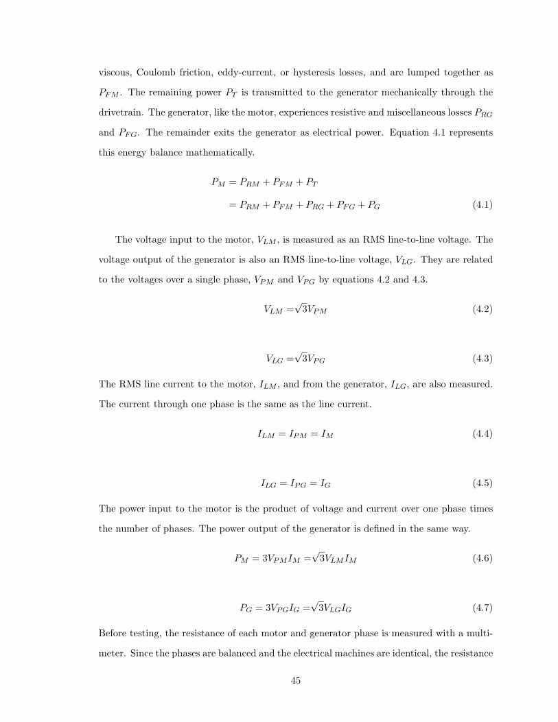
4.2 Power flows during each test run. . . . . . . . . . . . . . . . . . . . . . . . . 46
4.3 Generator frictional torque; data versus model. . . . . . . . . . . . . . . . . 48
4.4 Generator frictional losses; data versus model. . . . . . . . . . . . . . . . . . 49
4.5 Di!erence between modeled and measured frictional torque. . . . . . . . . . 50
4.6 Frictional power di!erence as a percentage of non-resistive power losses. . . 50
4.7 Generator phase current: modeled versus measured. . . . . . . . . . . . . . 61
4.8 Generator line voltage: modeled versus measured. . . . . . . . . . . . . . . . 62
4.9 Generator output power: modeled versus measured. . . . . . . . . . . . . . 62
4.10 Generator e"ciency: modeled versus measured. . . . . . . . . . . . . . . . . 63
4.11 Generator applied torque: modeled versus measured. . . . . . . . . . . . . . 63
4.12 Nameplate of the CE&P generator. . . . . . . . . . . . . . . . . . . . . . . . 64
A.1 Primary transistor specifications. . . . . . . . . . . . . . . . . . . . . . . . . 74
A.2 Secondary transistor specifications. . . . . . . . . . . . . . . . . . . . . . . . 75
A.3 Quadrature optical encoder specifications, page 1 of 2. . . . . . . . . . . . . 76
A.4 Quadrature optical encoder specifications, page 2 of 2. . . . . . . . . . . . . 77
A.5 Digital signal processor specifications, page 1 of 2. . . . . . . . . . . . . . . 78
A.6 Digital signal processor specifications, page 2 of 2. . . . . . . . . . . . . . . 79
A.7 Three-phase bridge rectifier specifications. . . . . . . . . . . . . . . . . . . . 80
A.8 Shunt resistor specifications. . . . . . . . . . . . . . . . . . . . . . . . . . . . 81
A.9 Operational amplifier specifications. . . . . . . . . . . . . . . . . . . . . . . 82
B.1 Dynamic C code, page 1 of 6. . . . . . . . . . . . . . . . . . . . . . . . . . . 84
B.2 Dynamic C code, page 2 of 6. . . . . . . . . . . . . . . . . . . . . . . . . . . 85
B.3 Dynamic C code, page 3 of 6. . . . . . . . . . . . . . . . . . . . . . . . . . . 86
B.4 Dynamic C code, page 4 of 6. . . . . . . . . . . . . . . . . . . . . . . . . . . 87
B.5 Dynamic C code, page 5 of 6. . . . . . . . . . . . . . . . . . . . . . . . . . . 88
B.6 Dynamic C code, page 6 of 6. . . . . . . . . . . . . . . . . . . . . . . . . . . 89
C.1 Raw data, page 1 of 2. . . . . . . . . . . . . . . . . . . . . . . . . . . . . . . 91
C.2 Raw data, page 2 of 2. . . . . . . . . . . . . . . . . . . . . . . . . . . . . . . 92
viii
List of Tables
2.1 Phase names and associated motor power connections. . . . . . . . . . . . . 15
2.2 DSP pins and their uses. . . . . . . . . . . . . . . . . . . . . . . . . . . . . . 30
3.1 Test plan in data sheet format. . . . . . . . . . . . . . . . . . . . . . . . . . 38
4.1 Frictional torque curve fit options . . . . . . . . . . . . . . . . . . . . . . . . 48
4.2 Dynamometer torque equation . . . . . . . . . . . . . . . . . . . . . . . . . 54
4.3 Generator current equation . . . . . . . . . . . . . . . . . . . . . . . . . . . 58
4.4 Generator applied torque equation . . . . . . . . . . . . . . . . . . . . . . . 59
4.5 Generator line voltage equation . . . . . . . . . . . . . . . . . . . . . . . . . 59
4.6 Generator power output equation . . . . . . . . . . . . . . . . . . . . . . . . 59
4.7 Generator e"ciency equation . . . . . . . . . . . . . . . . . . . . . . . . . . 60
4.8 Generator modeled versus measured variables . . . . . . . . . . . . . . . . . 61
ix

Acknowledgements
To everyone who helped make this project work, helped maintain my sanity when it didn’t,
and shared my excitement when it did: I give you my sincere thanks, and I owe you a beer.
‡ Thanks especially to Dan Kammen, for his part in creating such a wonderful com-
munity of people who care about making energy renewable and appropriate ‡ Dennis Lieu,
for infecting me with his passion for electromechanical devices ‡ Mike, Scott, and Pete,
for making Hesse Hall the most welcoming building on campus ‡ David Auslander, for his
patience during a time of microcontroller crisis ‡ David, the Rabbit Semiconductor guy, for
generously giving me $230 worth of assistance on a $215 purchase ‡ Tim, for his inspiration
and guidance in the realm of quotations ‡ Mick, for bringing the student shop to life with
learning and laughter ‡ Christian and Nate, for managing to always seem excited by my
progress ‡ Pete Schwartz, whose 6-o’clock poems brought a rare beam of sunlight into the
lab ‡ Jude, for keeping my ego in check on the tennis court ‡ and a very special thanks to
Dan Prull, for his companionship and guidance from start to finish–as well as a thanks in
advance for hiring me when he becomes a hot-shot professor. ‡
x

xi

Chapter 1
Introduction
Horizontal boosters. Alluvial dampers. Ow. That’s not it, bring me the Hy-drospanner. I don’t know how we’re going to get out of this one.
– Han Solo
1

Wind turbines are comprised of to two main subsystems: one, the rotor, captures wind
power and converts it to mechanical power. The second subsystem is the generator, which
converts that mechanical power into electricity. Of the two, rotor design is by far the sexier
pursuit: the rotor is the most visible part of the turbine and the part that interacts directly
with the wind, making its design essential for e!ective operation and aesthetic acceptance.
Proof of this is the number of rotor designs in existence. One design–the three-bladed
horizontal axis rotor–has become extremely popular, but it is by no means ubiquitous, nor
is every such rotor designed in the same way. But no less important to the e!ectiveness
of a wind turbine is the design of its generator. For one, the generator determines how
e"ciently mechanical power produced by the rotor is converted to electrical power. Even
more importantly, the generator determines how the rotor interacts with the wind, by
a!ecting how a specific electrical loading translates into mechanical loading of the rotor.
One generator might require a rotor to rotate quickly to reach a specific voltage, while a
di!erent generator could reach that same voltage at low speed. Depending on the design
of the rotor, either case could be ideal. It is crucial, then, that the generator and rotor be
designed in tandem, so they can work together most e!ectively.
Of course, it is impossible to design around a generator when that generator’s properties
are not well understood. This is especially true when a new generator is developed. A novel
generator must be characterized though testing; not just to guide its improvement, but
also to inform the design of the entire wind turbine it will be a part of. But even when
an o!-the-shelf generator is utilized, it is sometimes necessary to independently test the
generator’s performance, verifying that the generator behaves exactly as its manufacturer
claims.
Such was the case for California Energy and Power (CE&P), a startup company de-
veloping small vertical axis wind turbines. For their 1 kW prototype wind turbine, CE&P
obtained a set of generators from a manufacturer in China: Feng Hua Generators Ltd. of
Shen-Yeng. The Renewable and Appropriate Energy Laboratory (RAEL) was asked to test
these generators in November 2006, as part of a larger contract to test CE&P’s prototype
wind turbine. This need became even more critical in January 2007, when the prototype
2
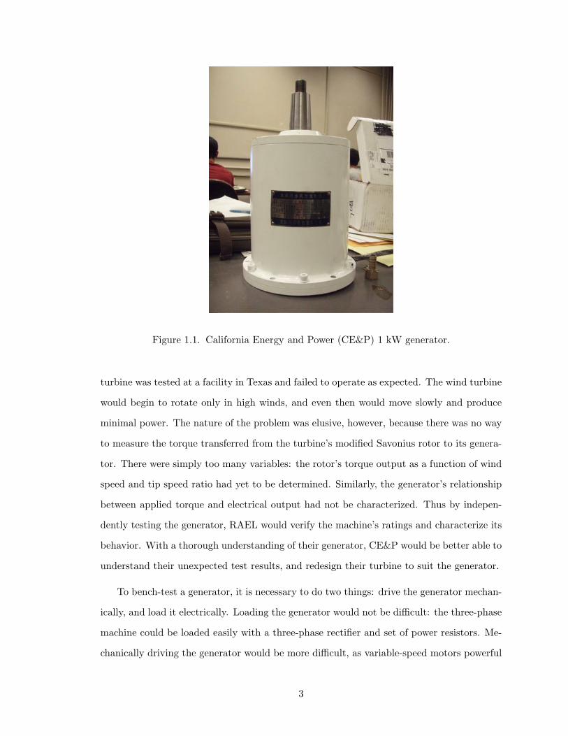
Figure 1.1. California Energy and Power (CE&P) 1 kW generator.
turbine was tested at a facility in Texas and failed to operate as expected. The wind turbine
would begin to rotate only in high winds, and even then would move slowly and produce
minimal power. The nature of the problem was elusive, however, because there was no way
to measure the torque transferred from the turbine’s modified Savonius rotor to its genera-
tor. There were simply too many variables: the rotor’s torque output as a function of wind
speed and tip speed ratio had yet to be determined. Similarly, the generator’s relationship
between applied torque and electrical output had not be characterized. Thus by indepen-
dently testing the generator, RAEL would verify the machine’s ratings and characterize its
behavior. With a thorough understanding of their generator, CE&P would be better able to
understand their unexpected test results, and redesign their turbine to suit the generator.
To bench-test a generator, it is necessary to do two things: drive the generator mechan-
ically, and load it electrically. Loading the generator would not be di"cult: the three-phase
machine could be loaded easily with a three-phase rectifier and set of power resistors. Me-
chanically driving the generator would be more di"cult, as variable-speed motors powerful
3
enough to drive a 1 kW generator are very expensive. Using a di!erent driving motor
would also create a paradox: how would this new motor be accurately characterized? For
these reasons, it was determined that the CE&P generator should be driven with a second
identical CE&P generator. One machine would be supplied power and driven as motor,
providing mechanical power to the second. The first advantage to this strategy is economic:
since two generators were available from CE&P, it was unnecessary to invest in another
electrical machine. The second advantage is technical: using two identical electrical ma-
chines would allow analysis of both machines to be performed simultaneously. The fact that
both machines should have the same properties–specifically motor constants and frictional
losses–would allow for a more accurate analysis.
The design challenge, then, was to build a system capable of driving a 3-phase, perma-
nent magnet CE&P generator as a variable-speed motor; transmitting its torque to a second
CE&P generator; and electrically loading the generator output with a variable resistance.
This system is referred to as a driving dynamometer, and its design is presented in Chap-
ter 2. Once the dynamometer was complete, it was used to perform preliminary testing in
a process described in Chapter 3. Next, Chapter 4 presents the analysis of the test data:
the theory behind it, the analysis itself, and its results. Lastly, Chapter 5 summarizes the
project, presents specific conclusions, and outlines future work.
4

Chapter 2
System Design
I had invested $14 and approximately an hour for research, development, andinstallation. In the collision the beer cans collapsed (as they were intended to);both my car and the Senate o"ce building remained splendidly unscathed.
– Victor PapanekDesign For the Real World
5

2.1 Overview
The purpose of the dynamometer system is to drive the CE&P permanent magnet
electrical generator at various speeds and various resistive loads, while electrical currents,
voltages, and rotational speed are measured. To accomplish this, an identical electrical
generator is operated as a motor, supplying mechanical power to the generator being tested.
Several subsystems make this possible, each of which is discussed in detail.
• Mounting Structure: A rigid platform holds both electrical machines steady during
testing. The platform is designed for high static and vibrational loads.
• Drivetrain: A chain drive conveys mechanical power from the motor to the generator.
• DC Power Supply: To reach adequate voltage, the system is powered by two DC
power supplies. These are connected in series and operated simultaneously.
• Power Electronics: A custom power electronics package is required to allow the
permanent magnet generator to operate as a motor.
• Control System: Continuous control of the motor is achieved through the use of an
optical encoder and a digital signal processor running Dynamic C code.
• Dump Load: The generator output is rectified and loaded with up to five power
resistors. A mounting structure holds the resistors securely in place.
• Measurement System: To adequately analyze the system, the system speed, input
and output voltage, and input and output currents must be measured.
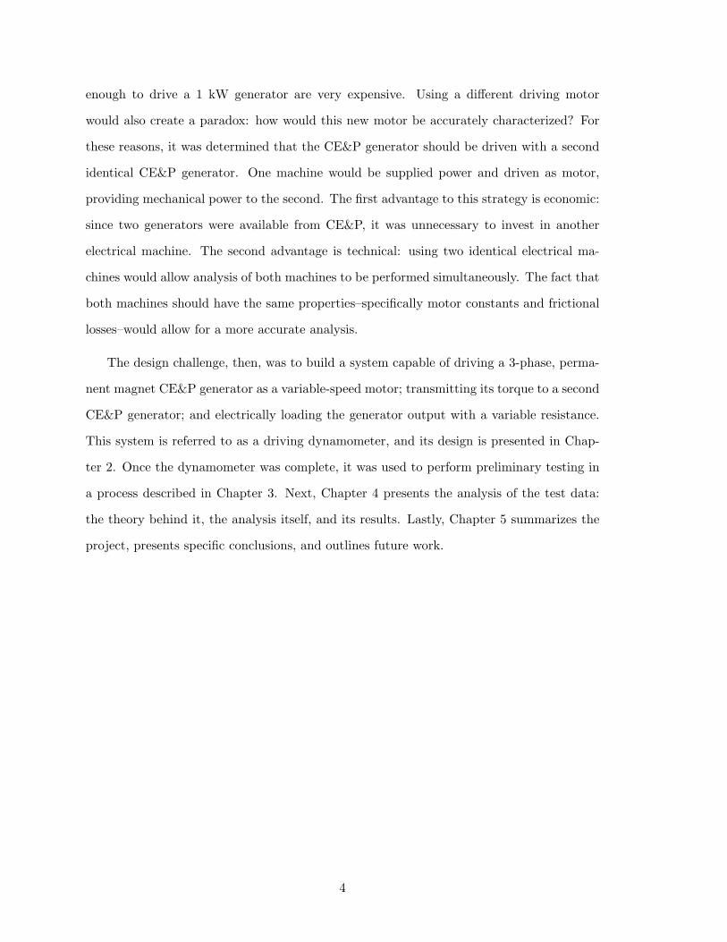
Figure 2.1 shows these systems and the flow of power and information between them.
Electrical power is supplied by the DC power supplies. The power electronics package
controls the flow of this power to phases of the motor, where the motor converts it to
mechanical power. The drivetrain transfers mechanical power to the generator, where it
is turned back into electricity and is dissipated in the dump load. To keep the motor
running smoothly, an optical encoder tracks the angular position of its shaft. Based on the
6
instantaneous shaft position, a digital signal processor determines which motor phases to
activate, and signals the power electronics package accordingly.
Figure 2.1. Subsystems comprising the driving dynamometer.
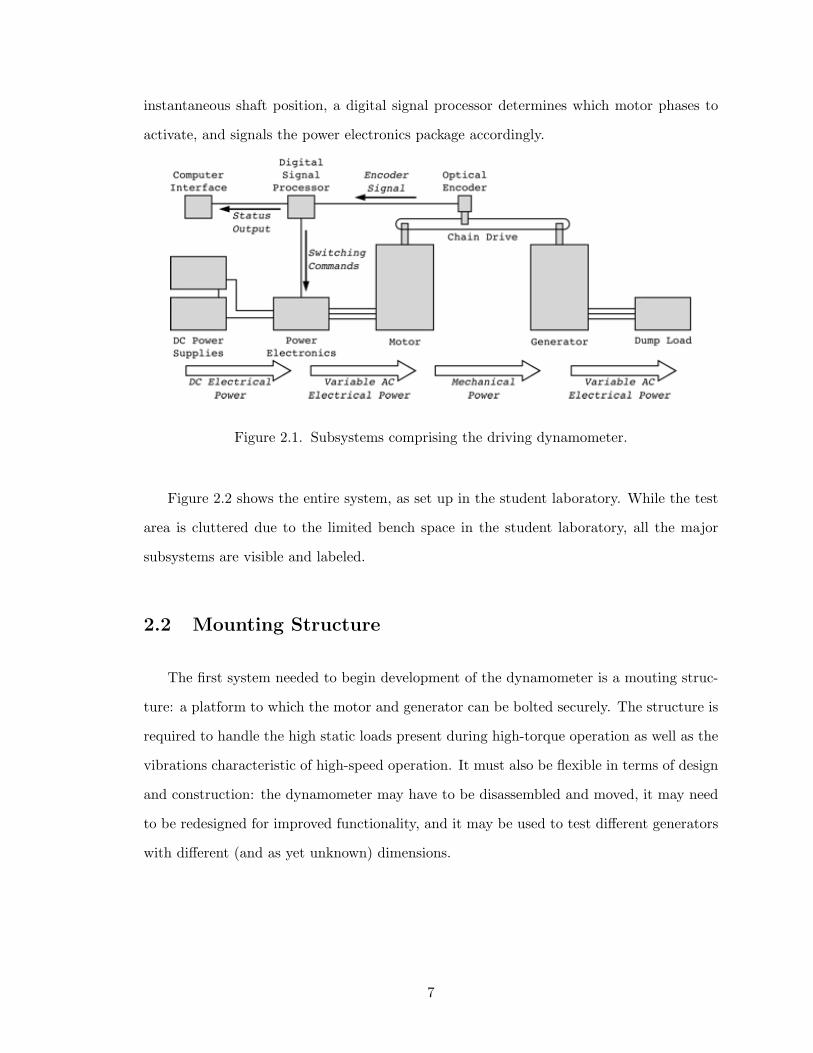
Figure 2.2 shows the entire system, as set up in the student laboratory. While the test
area is cluttered due to the limited bench space in the student laboratory, all the major
subsystems are visible and labeled.
2.2 Mounting Structure
The first system needed to begin development of the dynamometer is a mouting struc-
ture: a platform to which the motor and generator can be bolted securely. The structure is
required to handle the high static loads present during high-torque operation as well as the
vibrations characteristic of high-speed operation. It must also be flexible in terms of design
and construction: the dynamometer may have to be disassembled and moved, it may need
to be redesigned for improved functionality, and it may be used to test di!erent generators
with di!erent (and as yet unknown) dimensions.
7
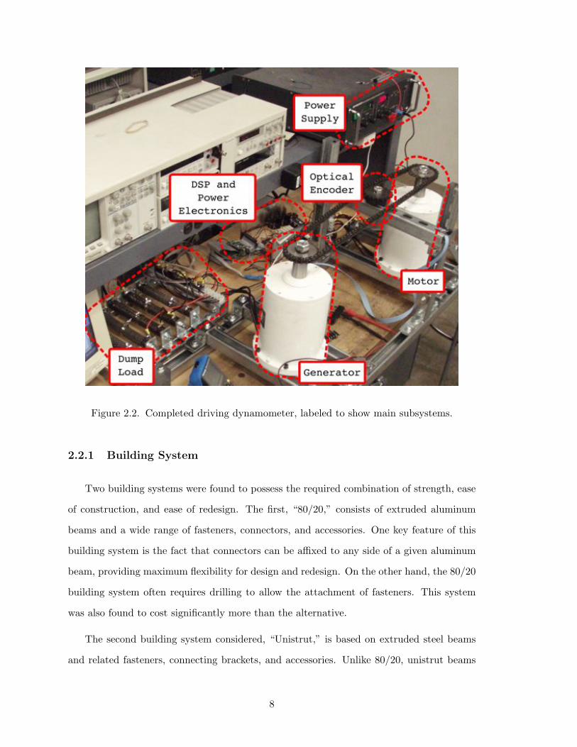
Figure 2.2. Completed driving dynamometer, labeled to show main subsystems.
2.2.1 Building System
Two building systems were found to possess the required combination of strength, ease
of construction, and ease of redesign. The first, “80/20,” consists of extruded aluminum
beams and a wide range of fasteners, connectors, and accessories. One key feature of this
building system is the fact that connectors can be a"xed to any side of a given aluminum
beam, providing maximum flexibility for design and redesign. On the other hand, the 80/20
building system often requires drilling to allow the attachment of fasteners. This system
was also found to cost significantly more than the alternative.
The second building system considered, “Unistrut,” is based on extruded steel beams
and related fasteners, connecting brackets, and accessories. Unlike 80/20, unistrut beams
8
consist of only one deep channel, so connections can be made on one side of a beam only.
However, that limitation does not pose a significant problem for this application, due to the
simplicity of the mounting structure and the variety of connecting brackets available. In
addition, Unistrut members require no machining to make connections. The system is also
significantly more economical than the 80/20 building system. For these reasons, Unistrut
was selected over 80/20 for construction of the mounting structure.
2.2.2 Basic Design
The design of the mounting structure was complicated by the fact that the permanent
magnet generators obtained from CE&P are designed for use in vertical-axis wind turbines.
When mounted on a horizontal surface, their shafts extend up vertically, rather than extend-
ing out horizontally. Thus the simplest solution–mounting the generators on a horizontal
surfact and connecting their shafts directly–was not an option. With this limitation in mind,
two mounting options were considered. First, the shafts chould be connected directly with
a shaft coupling if the generators were mounted to extend horizontally, facing each other
on parallel upright surfaces. On the other hand, the generators could be mounted on the
same horizontal surface, extending vertically. In this case, the shafts cannot be connected
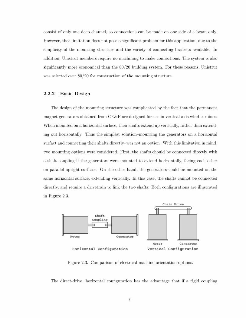
directly, and require a drivetrain to link the two shafts. Both configurations are illustrated
in Figure 2.3.
Figure 2.3. Comparison of electrical machine orientation options.
The direct-drive, horizontal configuration has the advantage that if a rigid coupling
9
is used, frictional losses between the two machines are entirely eliminated. The vertical
configuration, however, has even more important advantages. For one, it requires a much
simpler mounting structure, since the 75-lb motors rest directly on the platform rather than
being cantilevered out towards each other. Similarly, the vertical configuration simplifies
assembly: while mounting or dismounting an electrical machine, it is not necessary to fight
gravity while getting the machine into position. While the introduction of a chain drive
is an additional system and expense, it confers two more advantages. First, it simplifies
alignment. Since the shafts are not connected directly, they need not be perfectly aligned.
Second, it introduces an opportunity for easy and e!ective position sensing. While the
chain drive keeps the motor and generator turning in unison, it can also turn a sprocket-
mounted optical encoder. In the horizontal configuration, an additional drivetrain would be
required to link the shafts to the optical encoder–thus making it no simpler than the vertical
configuration. For these reasons, the vertical configuration is selected for the dynamometer.
2.2.3 Additional Design Considerations
To ensure proper tensioning of the roller chain, and to allow easy disassembly of the
system, the generator mount is designed to rest on rolling trolleys that move within the main
horizontal channels. Thus during disassembly, the generator’s mount can be untightened
and rolled towards the motor to create slack in the drive chain. For reassembly, the generator
is pulled away from motor to lightly preload the chain while the mount is tighened securely
down for testing. The rolling trolleys must withstand the compressive force of the generator,
as well as an additional compressive force introduced when the generator mount is tightened
down. Distributed among four trolleys, the total force on generator mount can safely
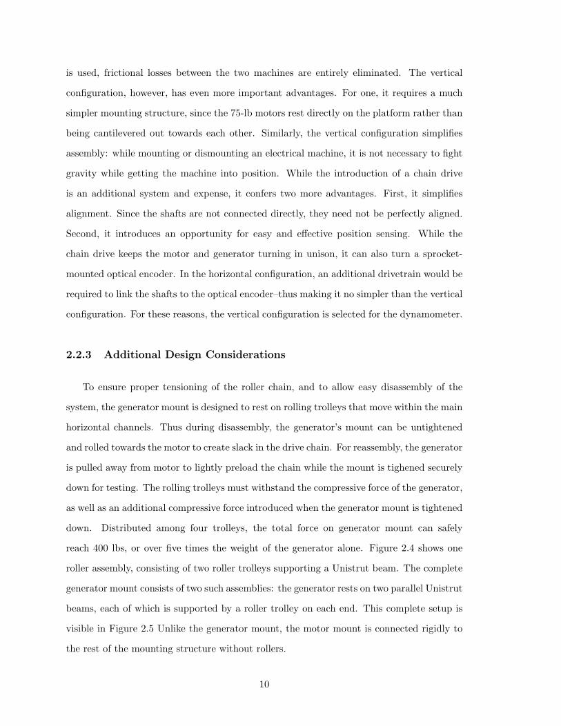
reach 400 lbs, or over five times the weight of the generator alone. Figure 2.4 shows one
roller assembly, consisting of two roller trolleys supporting a Unistrut beam. The complete
generator mount consists of two such assemblies: the generator rests on two parallel Unistrut
beams, each of which is supported by a roller trolley on each end. This complete setup is
visible in Figure 2.5 Unlike the generator mount, the motor mount is connected rigidly to
the rest of the mounting structure without rollers.
10
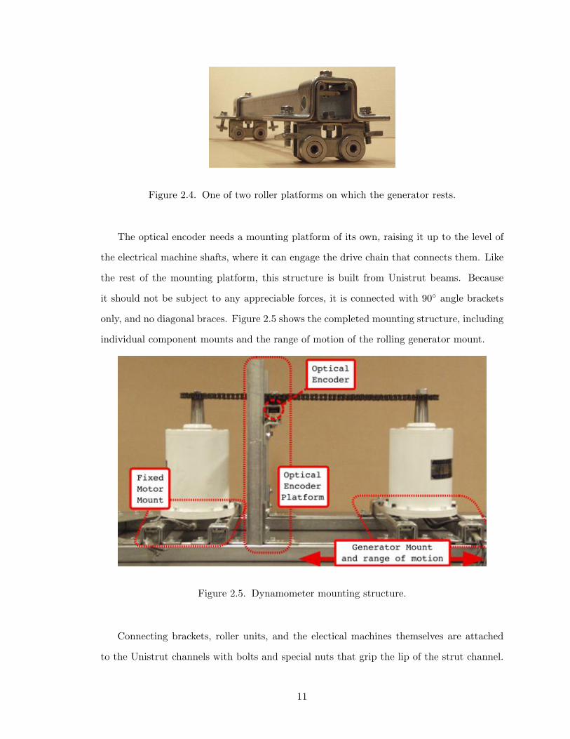
Figure 2.4. One of two roller platforms on which the generator rests.
The optical encoder needs a mounting platform of its own, raising it up to the level of
the electrical machine shafts, where it can engage the drive chain that connects them. Like
the rest of the mounting platform, this structure is built from Unistrut beams. Because
it should not be subject to any appreciable forces, it is connected with 90! angle brackets
only, and no diagonal braces. Figure 2.5 shows the completed mounting structure, including
individual component mounts and the range of motion of the rolling generator mount.
Figure 2.5. Dynamometer mounting structure.
Connecting brackets, roller units, and the electical machines themselves are attached
to the Unistrut channels with bolts and special nuts that grip the lip of the strut channel.
11
To ensure that connections remain secure throughout potentially vibration-prone testing,
split-ring lock washers are used with every fastener.
2.3 Drivetrain
2.3.1 Theory
When the dynamometer is running, It is essential for both electrical machines and
the encoder to rotate exactly synchronously. If the generator alone turns at a di!erent
di!erent angular velocity, the speed measurement developed by the encoder and digital
signal processor will inaccurately reflect the true speed of the generator. Worse still, if the
encoder and motor get out of sync the motor will stop turning smoothly, jerk to a halt, or
move erratically with potentially dangerous torque and current.
Thus a belt and pully system would be inadequate. Belts can have a tendency to slip
(suddenly losing traction) and creep (slowly advancing one pulley faster than another).
Chain drive systems, however, guarantee sychronous motion by engaging discrete chain
links on the teeth of a sprocket. As long as each sprocket has the same number of teeth and
the chain does not fail, the motion of each component will remain synchronous indefinitely.
2.3.2 Design
The generator shafts are designed for an attachment to be bolted on, compressed be-
tween the thick main shaft and a nut on the thinner, threaded end of the shaft. The thread
is an unusual metric size: 20 mm in diameter, with a 1.5 mm pitch. Thus to fit the shafts,
flat sprockets with a 5/8” (15.9 mm) bore were machined on a lathe to have the required
20 mm bore. Figure 2.6 shows a sprocket mounted on the generator shaft.
The shaft of the optical encoder is 1/4”, far too small for any standard sprocket. This
problem was solved by increasing the diameter of the shaft with aluminum shaft couplings.
These inexpensive units attach with set screws, and are adequate for the low torque applied
to the encoder. One coupling has an inside diameter of 1/4” and and outside diamter of
12
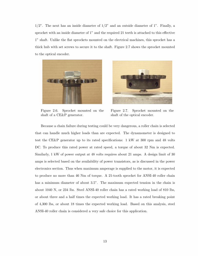
1/2”. The next has an inside diameter of 1/2” and an outside diameter of 1”. Finally, a
sprocket with an inside diameter of 1” and the required 21 teeth is attached to this e!ective
1” shaft. Unlike the flat sprockets mounted on the electrical machines, this sprocket has a
thick hub with set screws to secure it to the shaft. Figure 2.7 shows the sprocket mounted
to the optical encoder.
Figure 2.6. Sprocket mounted on theshaft of a CE&P generator.
Figure 2.7. Sprocket mounted on theshaft of the optical encoder.
Because a chain failure during testing could be very dangerous, a roller chain is selected
that can handle much higher loads than are expected. The dynamometer is designed to
test the CE&P generator up to its rated specifications: 1 kW at 300 rpm and 48 volts
DC. To produce this rated power at rated speed, a torque of about 32 Nm is expected.
Similarly, 1 kW of power output at 48 volts requires about 21 amps. A design limit of 30
amps is selected based on the availability of power transistors, as is discussed in the power
electronics section. Thus when maximum amperage is supplied to the motor, it is expected
to produce no more than 46 Nm of torque. A 21-tooth sprocket for ANSI-40 roller chain
has a minimum diameter of about 3.5”. The maximum expected tension in the chain is
about 1040 N, or 234 lbs. Steel ANSI-40 roller chain has a rated working load of 810 lbs,
or about three and a half times the expected working load. It has a rated breaking point
of 4,300 lbs, or about 18 times the expected working load. Based on this analysis, steel
ANSI-40 roller chain is considered a very safe choice for this application.
13
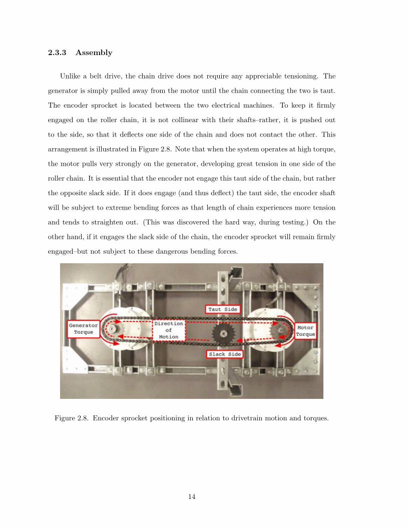
2.3.3 Assembly
Unlike a belt drive, the chain drive does not require any appreciable tensioning. The
generator is simply pulled away from the motor until the chain connecting the two is taut.
The encoder sprocket is located between the two electrical machines. To keep it firmly
engaged on the roller chain, it is not collinear with their shafts–rather, it is pushed out
to the side, so that it deflects one side of the chain and does not contact the other. This
arrangement is illustrated in Figure 2.8. Note that when the system operates at high torque,
the motor pulls very strongly on the generator, developing great tension in one side of the
roller chain. It is essential that the encoder not engage this taut side of the chain, but rather
the opposite slack side. If it does engage (and thus deflect) the taut side, the encoder shaft
will be subject to extreme bending forces as that length of chain experiences more tension
and tends to straighten out. (This was discovered the hard way, during testing.) On the
other hand, if it engages the slack side of the chain, the encoder sprocket will remain firmly
engaged–but not subject to these dangerous bending forces.
Figure 2.8. Encoder sprocket positioning in relation to drivetrain motion and torques.
14
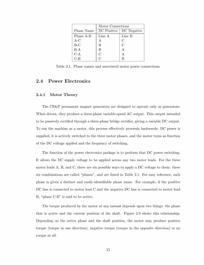
Motor ConnectionsPhase Name DC Positive DC NegativePhase A-B Line A Line BA-C A CB-C B CB-A B AC-A C AC-B C B
Table 2.1. Phase names and associated motor power connections.
2.4 Power Electronics
2.4.1 Motor Theory
The CE&P permanent magnet generators are designed to operate only as generators.
When driven, they produce a three-phase variable-speed AC output. This output intended
to be passively rectified through a three-phase bridge rectifier, giving a variable DC output.
To run the machine as a motor, this process e!ectively proceeds backwards: DC power is
supplied, it is actively switched to the three motor phases, and the motor turns as function
of the DC voltage applied and the frequency of switching.
The function of the power electronics package is to perform that DC power switching.
It allows the DC supply voltage to be applied across any two motor leads. For the three
motor leads A, B, and C, there are six possible ways to apply a DC voltage to them: these
six combinations are called “phases”, and are listed in Table 2.1. For easy reference, each
phase is given a distinct and easily-identifiable phase name. For example, if the positive
DC line is connected to motor lead C and the negative DC line is connected to motor lead
B, “phase C-B” is said to be active.
The torque produced by the motor at any instant depends upon two things: the phase
that is active and the current position of the shaft. Figure 2.9 shows this relationship.
Depending on the active phase and the shaft position, the motor may produce positive
torque (torque in one direction), negative torque (torque in the opposite direction) or no
torque at all.
15
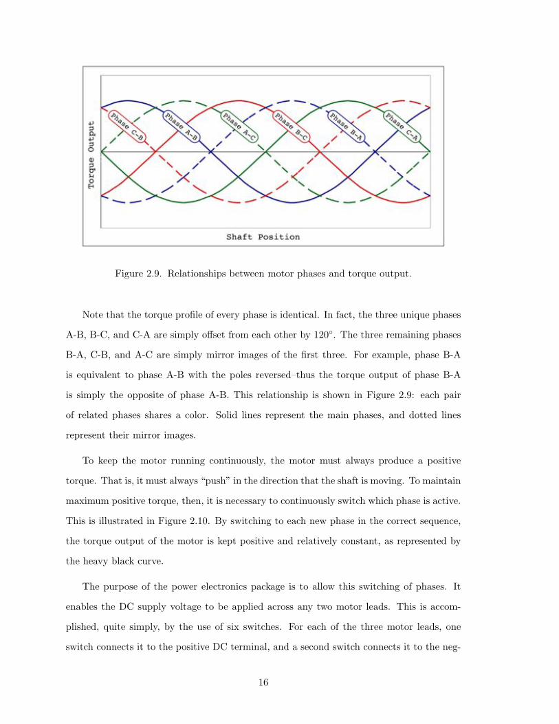
Figure 2.9. Relationships between motor phases and torque output.
Note that the torque profile of every phase is identical. In fact, the three unique phases
A-B, B-C, and C-A are simply o!set from each other by 120!. The three remaining phases
B-A, C-B, and A-C are simply mirror images of the first three. For example, phase B-A
is equivalent to phase A-B with the poles reversed–thus the torque output of phase B-A
is simply the opposite of phase A-B. This relationship is shown in Figure 2.9: each pair
of related phases shares a color. Solid lines represent the main phases, and dotted lines
represent their mirror images.
To keep the motor running continuously, the motor must always produce a positive
torque. That is, it must always “push” in the direction that the shaft is moving. To maintain
maximum positive torque, then, it is necessary to continuously switch which phase is active.
This is illustrated in Figure 2.10. By switching to each new phase in the correct sequence,
the torque output of the motor is kept positive and relatively constant, as represented by
the heavy black curve.
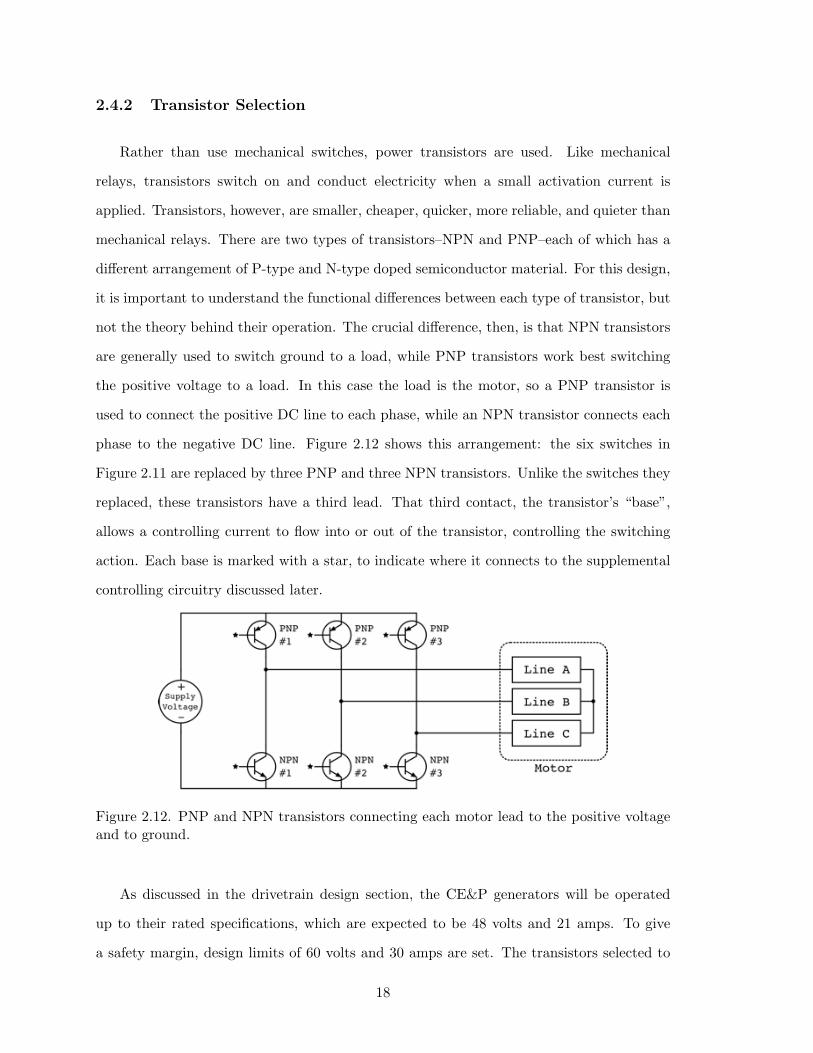
The purpose of the power electronics package is to allow this switching of phases. It
enables the DC supply voltage to be applied across any two motor leads. This is accom-
plished, quite simply, by the use of six switches. For each of the three motor leads, one
switch connects it to the positive DC terminal, and a second switch connects it to the neg-
16
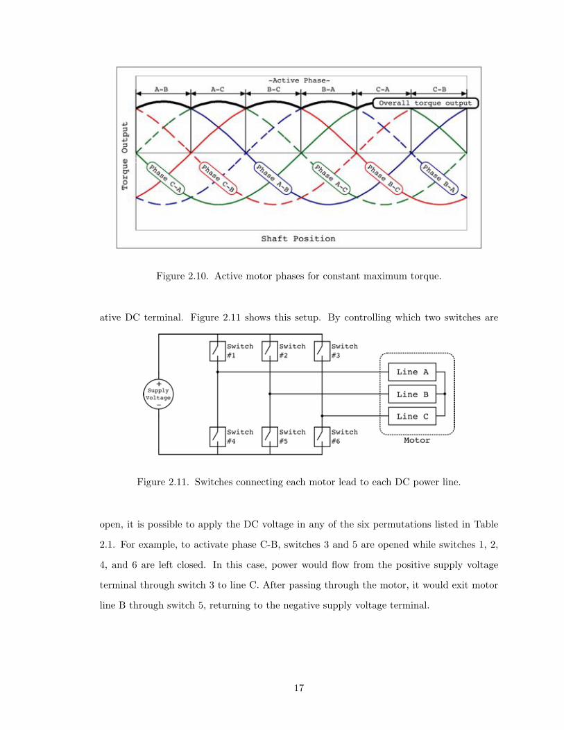
Figure 2.10. Active motor phases for constant maximum torque.
ative DC terminal. Figure 2.11 shows this setup. By controlling which two switches are
Figure 2.11. Switches connecting each motor lead to each DC power line.
open, it is possible to apply the DC voltage in any of the six permutations listed in Table
2.1. For example, to activate phase C-B, switches 3 and 5 are opened while switches 1, 2,
4, and 6 are left closed. In this case, power would flow from the positive supply voltage
terminal through switch 3 to line C. After passing through the motor, it would exit motor
line B through switch 5, returning to the negative supply voltage terminal.
17
2.4.2 Transistor Selection
Rather than use mechanical switches, power transistors are used. Like mechanical
relays, transistors switch on and conduct electricity when a small activation current is
applied. Transistors, however, are smaller, cheaper, quicker, more reliable, and quieter than
mechanical relays. There are two types of transistors–NPN and PNP–each of which has a
di!erent arrangement of P-type and N-type doped semiconductor material. For this design,
it is important to understand the functional di!erences between each type of transistor, but
not the theory behind their operation. The crucial di!erence, then, is that NPN transistors
are generally used to switch ground to a load, while PNP transistors work best switching
the positive voltage to a load. In this case the load is the motor, so a PNP transistor is
used to connect the positive DC line to each phase, while an NPN transistor connects each
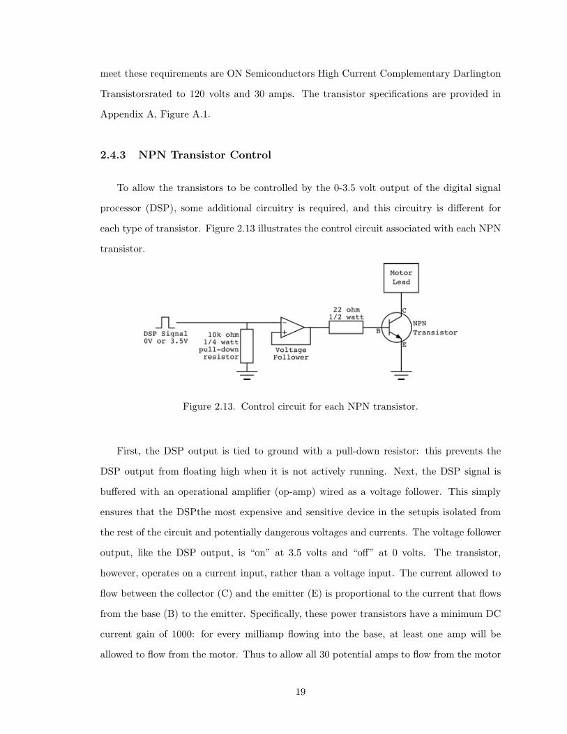
phase to the negative DC line. Figure 2.12 shows this arrangement: the six switches in
Figure 2.11 are replaced by three PNP and three NPN transistors. Unlike the switches they
replaced, these transistors have a third lead. That third contact, the transistor’s “base”,
allows a controlling current to flow into or out of the transistor, controlling the switching
action. Each base is marked with a star, to indicate where it connects to the supplemental
controlling circuitry discussed later.
Figure 2.12. PNP and NPN transistors connecting each motor lead to the positive voltageand to ground.
As discussed in the drivetrain design section, the CE&P generators will be operated
up to their rated specifications, which are expected to be 48 volts and 21 amps. To give
a safety margin, design limits of 60 volts and 30 amps are set. The transistors selected to
18
meet these requirements are ON Semiconductors High Current Complementary Darlington
Transistorsrated to 120 volts and 30 amps. The transistor specifications are provided in
Appendix A, Figure A.1.
2.4.3 NPN Transistor Control
To allow the transistors to be controlled by the 0-3.5 volt output of the digital signal
processor (DSP), some additional circuitry is required, and this circuitry is di!erent for
each type of transistor. Figure 2.13 illustrates the control circuit associated with each NPN
transistor.
Figure 2.13. Control circuit for each NPN transistor.
First, the DSP output is tied to ground with a pull-down resistor: this prevents the
DSP output from floating high when it is not actively running. Next, the DSP signal is
bu!ered with an operational amplifier (op-amp) wired as a voltage follower. This simply
ensures that the DSPthe most expensive and sensitive device in the setupis isolated from
the rest of the circuit and potentially dangerous voltages and currents. The voltage follower
output, like the DSP output, is “on” at 3.5 volts and “o!” at 0 volts. The transistor,
however, operates on a current input, rather than a voltage input. The current allowed to
flow between the collector (C) and the emitter (E) is proportional to the current that flows
from the base (B) to the emitter. Specifically, these power transistors have a minimum DC
current gain of 1000: for every milliamp flowing into the base, at least one amp will be
allowed to flow from the motor. Thus to allow all 30 potential amps to flow from the motor
19
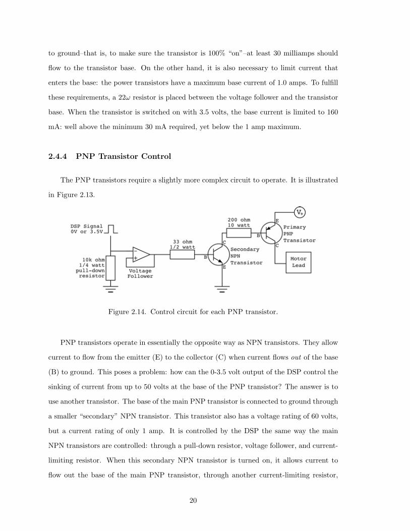
to ground–that is, to make sure the transistor is 100% “on”–at least 30 milliamps should
flow to the transistor base. On the other hand, it is also necessary to limit current that
enters the base: the power transistors have a maximum base current of 1.0 amps. To fulfill
these requirements, a 22! resistor is placed between the voltage follower and the transistor
base. When the transistor is switched on with 3.5 volts, the base current is limited to 160
mA: well above the minimum 30 mA required, yet below the 1 amp maximum.
2.4.4 PNP Transistor Control
The PNP transistors require a slightly more complex circuit to operate. It is illustrated
in Figure 2.13.
Figure 2.14. Control circuit for each PNP transistor.
PNP transistors operate in essentially the opposite way as NPN transistors. They allow
current to flow from the emitter (E) to the collector (C) when current flows out of the base
(B) to ground. This poses a problem: how can the 0-3.5 volt output of the DSP control the
sinking of current from up to 50 volts at the base of the PNP transistor? The answer is to
use another transistor. The base of the main PNP transistor is connected to ground through
a smaller “secondary” NPN transistor. This transistor also has a voltage rating of 60 volts,
but a current rating of only 1 amp. It is controlled by the DSP the same way the main
NPN transistors are controlled: through a pull-down resistor, voltage follower, and current-
limiting resistor. When this secondary NPN transistor is turned on, it allows current to
flow out the base of the main PNP transistor, through another current-limiting resistor,
20
and to ground. This current flow allows the PNP transistor to open, sending the positive
DC voltage to that motor lead. When the DSP signal drops to zero, the NPN resistor shuts
o!: current cannot flow from the PNP transistor’s base, so the PNP transistor shuts o! as
well. The secondary NPN transistor specifications are given in Appendix A, Figure A.2.
2.4.5 Additional Circuit Design
To facilitate development and troubleshooting, the DSP outputs are also fed to an LED
array. This array consists of two rows of three LEDs, representing the six switches that
control the motor. Whenever a switch is activated, the corresponding LED is illuminated.
Because the amount of current supplied by each op-amp is limited, each LED is bu!ered
through its own voltage follower. In this way, the lighting circuit is guaranteed not to
interfere with the current requirements of the switching circuit.
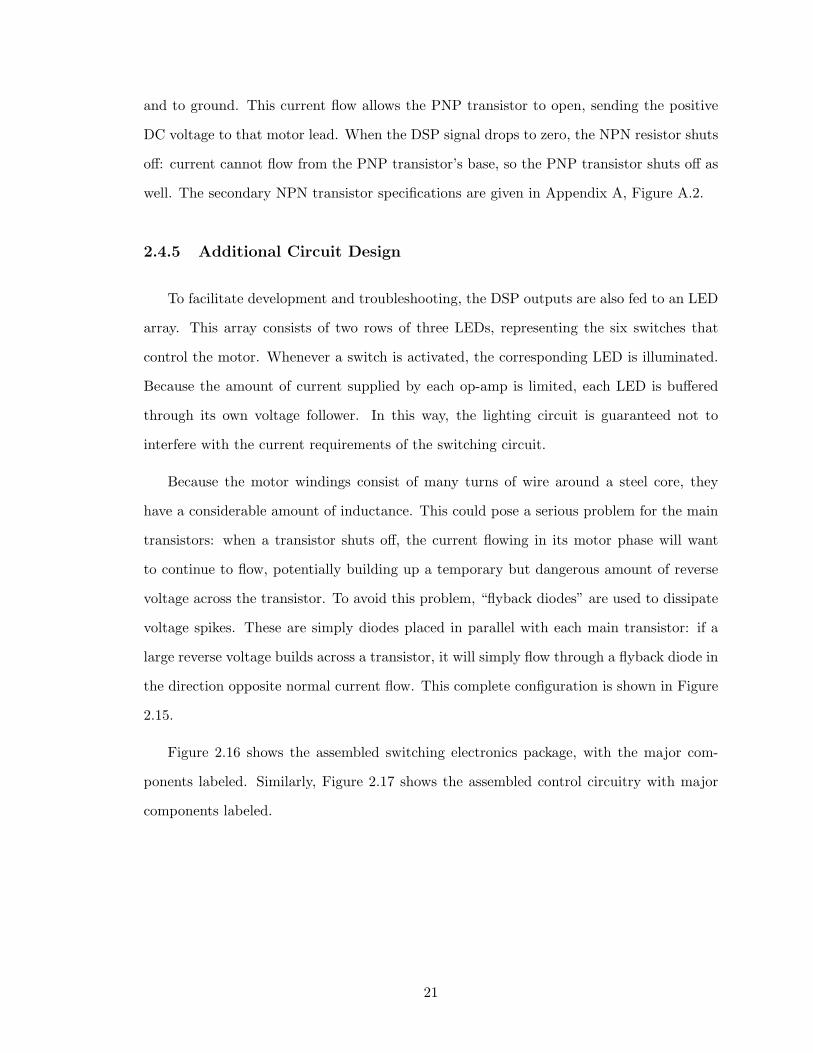
Because the motor windings consist of many turns of wire around a steel core, they
have a considerable amount of inductance. This could pose a serious problem for the main
transistors: when a transistor shuts o!, the current flowing in its motor phase will want
to continue to flow, potentially building up a temporary but dangerous amount of reverse
voltage across the transistor. To avoid this problem, “flyback diodes” are used to dissipate
voltage spikes. These are simply diodes placed in parallel with each main transistor: if a
large reverse voltage builds across a transistor, it will simply flow through a flyback diode in
the direction opposite normal current flow. This complete configuration is shown in Figure
2.15.
Figure 2.16 shows the assembled switching electronics package, with the major com-
ponents labeled. Similarly, Figure 2.17 shows the assembled control circuitry with major
components labeled.
21
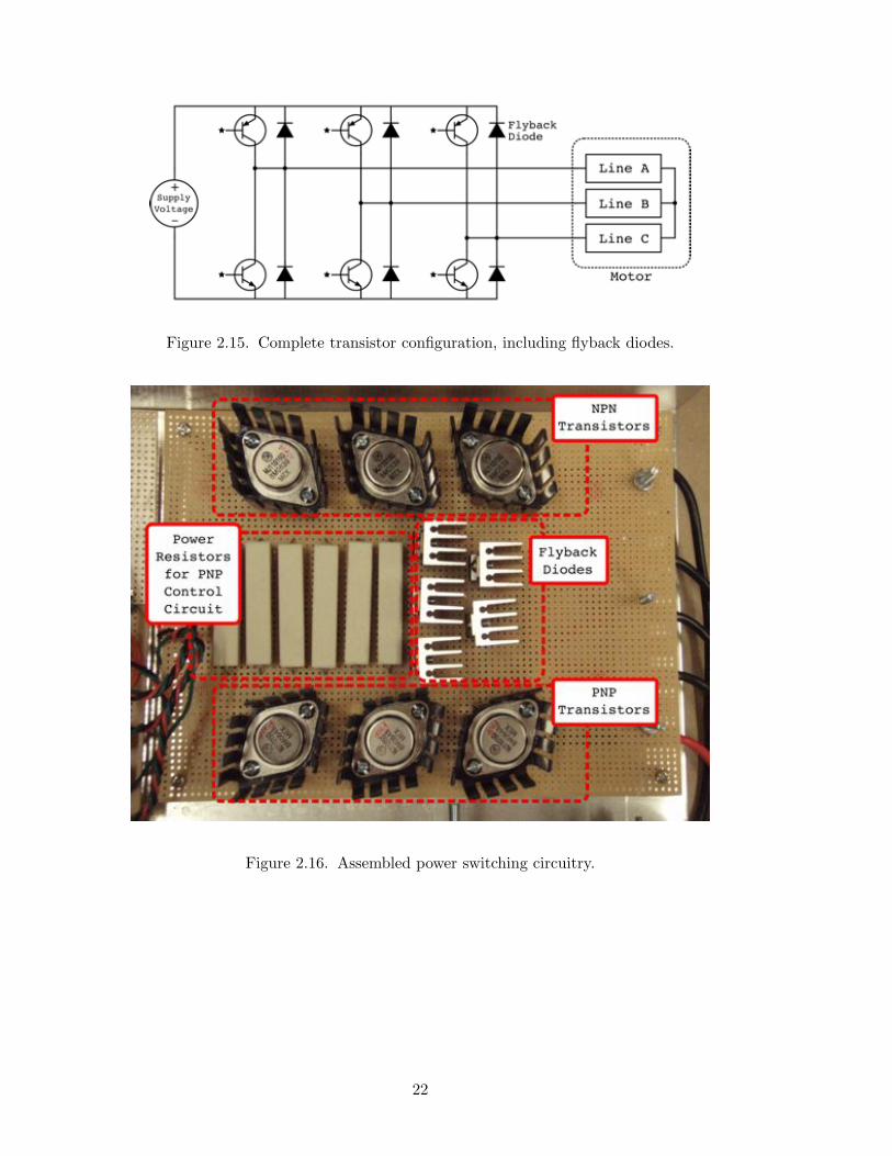
Figure 2.15. Complete transistor configuration, including flyback diodes.
Figure 2.16. Assembled power switching circuitry.
22
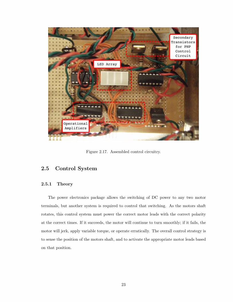
Figure 2.17. Assembled control circuitry.
2.5 Control System
2.5.1 Theory
The power electronics package allows the switching of DC power to any two motor
terminals, but another system is required to control that switching. As the motors shaft
rotates, this control system must power the correct motor leads with the correct polarity
at the correct times. If it succeeds, the motor will continue to turn smoothly; if it fails, the
motor will jerk, apply variable torque, or operate erratically. The overall control strategy is
to sense the position of the motors shaft, and to activate the appropriate motor leads based
on that position.
23
2.5.2 Control Strategy
A high-resolution quadrature encoder is used to track the position of the motor shaft.
As it turns, the encoder produces two square-wave pulses–o!set by 90!–that correspond to
its movement. A decoder within the DSP interprets that signal, and converts it to an integer
count. As the encoder moves in one direction, the count increments every 0.35 degrees–
or 1024 times per revolution. If the encoder moves in the opposite direction, the count
decreases. Thus the encoder does not report absolute position, only the relative position
of the shaft. It also does not reset its count to zero each revolution. Instead, it counts
continuously up.
An absolute shaft position must be determined, however, because power must be
switched to various motor phases at fixed angular positions of the motor shaft. To pro-
duce an absolute position, the encoder is first initialized at a known position, in a process
that is outlined in section 2.5.3 below. Next, the true encoder count is modulated to 1024,
the number of encoder counts in one revolution. Thus even as the encoder completes multi-
ple revolutions and the count far exceeds 1024, the absolute shaft position is always tracked
as a number between zero and 1024.
Thus a number is obtained that corresponds to the instantaneous position of the motor
shaft. To make use of this number, the locations where phase switching should take place
must also be associated with a number. These locations are dubbed “switch points,” because
they are the shaft positions where phase switching should occur. Once the switch points
are associated with integers, the DSP can determine which motor phase to activate simply
by comparing two integers.
Figure 2.18 illustrates this control strategy. Say the encoder returns a current position
38. This value is between 35 and 76, so phase A-C is activated: the DSP signals the
transistors associated with phase A-C to open, connecting motor line A to the positive DC
terminal and motor line C to the negative DC terminal. Later, the encoder may return
a value of 95: again this value is compared to the values associated with each switch
point. Since it is between 76 and 104, phase B-C should be activated. This process repeats
24
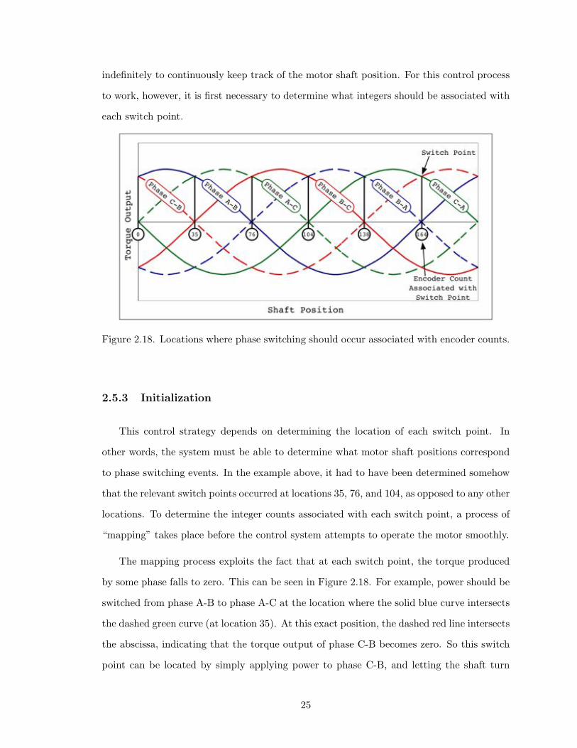
indefinitely to continuously keep track of the motor shaft position. For this control process
to work, however, it is first necessary to determine what integers should be associated with
each switch point.
Figure 2.18. Locations where phase switching should occur associated with encoder counts.
2.5.3 Initialization
This control strategy depends on determining the location of each switch point. In
other words, the system must be able to determine what motor shaft positions correspond
to phase switching events. In the example above, it had to have been determined somehow
that the relevant switch points occurred at locations 35, 76, and 104, as opposed to any other
locations. To determine the integer counts associated with each switch point, a process of
“mapping” takes place before the control system attempts to operate the motor smoothly.
The mapping process exploits the fact that at each switch point, the torque produced
by some phase falls to zero. This can be seen in Figure 2.18. For example, power should be
switched from phase A-B to phase A-C at the location where the solid blue curve intersects
the dashed green curve (at location 35). At this exact position, the dashed red line intersects
the abscissa, indicating that the torque output of phase C-B becomes zero. So this switch
point can be located by simply applying power to phase C-B, and letting the shaft turn
25
until it stops. When the shafts stops, the encoder is sampled and its reading–in this case
35–is stored. The next switch point is located in the same way: the next phase, phase A-B,
is powered. Again the motor shaft will turn, and eventually stop. This new location is
associated with switching from phase A-C to phase B-C. The process of stepping, waiting,
encoder sampling, and storing is repeated for an entire revolution.
The CE&P generator is a 10-pole machine. For each pair of poles, the machine experi-
ences one full electrical cycle, where one cycle consists of all six phase transitions as shown
in Figure 2.18 above. Thus for each revolution of the motor shaft, the motor must e!ect five
sets of six transitions, or 30 phase transitions. The process of mapping, then, continues for
one full revolution, logging thirty switch point locations, each of which is a number between
zero and 1024.
Once the motor completes this initialization sequence, it immediately enters the normal
running mode. In this mode, the DSP constantly compares the encoder position to the
mapped positions, changing phase when necessary to maintain smooth operation.
2.5.4 Motor Speed
Nowhere in the control strategy is the motor speed addressed, because the motor speed
is not determined by the control system. Instead, the motor speed is controlled by the
voltage of the DC power supply. If the DC input is low, the motor will advance from one
switch point to the next slowly (but still smoothly). If a higher voltage is applied, the motor
will turn more quickly. Because the control system makes phase switches as a function of
shaft position (as opposed to a timed schedule), it automatically adjusts the frequency of
phase switching to match any motor speed, as determined by the voltage input.
2.5.5 Speed Measurement
Because the motor speed is not directly controlled, it must be measured. This is done
by reusing the information provided by the encoder. Once a second, the encoder count
countN is logged and compared to the encoder count one second before, countN"1. The
26
di!erence is divided by the one second time interval, and scaled to give a speed reading in
revolutions per minute, as shown in Equation 2.1.
!rpm =60 sec/min
1024 counts/rev
countN " countN"1
1 sec(2.1)
The motor speed reading must be noted in real time during testing, so it is output from
the DSP to a PC serial port. By using the program Hyperterminal on the PC, the speed is
read from the serial port and displayed on-screen in real time.
2.5.6 Frequency Considerations
To operate smoothly at all speeds, the control system must be able to keep up with the
required motor switching frequency. Specifically, the control system should always run at
least two cycles for each switching operation, where one cycle consists of reading the encoder
and activating the corresponding phase. The CE&P generators have a rated speed of 300
rpm. Given 30 switch points per revolution, the motor will require 150 switching operations
per second at that speed. For the control system to operate at twice that frequency, it must
run at at least 300 Hz, sampling at least once every 3.3 milliseconds.
The first solution to this challenge was to run the control system with a timer and a
tight loop. That is, sampling events would be scheduled every, say, 2 ms. An empty while(
) loop would simply idle until a scheduled time, at which point the encoder-sampling and
phase-switching process would take place. As long as this sequence finished in less than
2 ms, the scheduled timing would be maintained. Unfortunately, one essential command
takes the DSP more than 2 ms to complete, disrupting the timing. This is the puts( )
(literally, “put string”) command that enables the speed to be communicated to the PC
and displayed in real time. That command alone was found to take about 3.5 to 4 ms to
complete, making impossible to maintain the 3.3 ms minimum sampling frequency.
A new solution was devised using the slice( ) command available in the Dynamic C
programming language used by the DSP. This function allows long processes like the puts(
) command to be paused while other commands run, and re-started when there is another
opportunity. It is based on the idea that segments of code can be separated into “slices,”
27
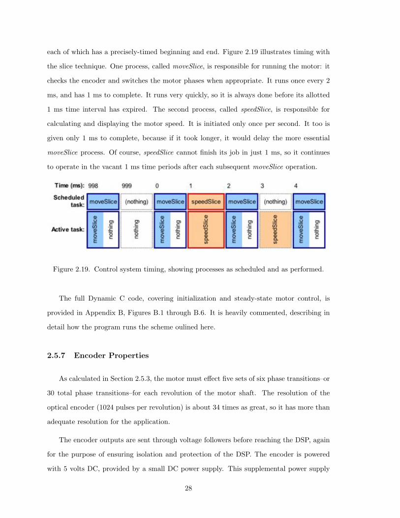
each of which has a precisely-timed beginning and end. Figure 2.19 illustrates timing with
the slice technique. One process, called moveSlice, is responsible for running the motor: it
checks the encoder and switches the motor phases when appropriate. It runs once every 2
ms, and has 1 ms to complete. It runs very quickly, so it is always done before its allotted
1 ms time interval has expired. The second process, called speedSlice, is responsible for
calculating and displaying the motor speed. It is initiated only once per second. It too is
given only 1 ms to complete, because if it took longer, it would delay the more essential
moveSlice process. Of course, speedSlice cannot finish its job in just 1 ms, so it continues
to operate in the vacant 1 ms time periods after each subsequent moveSlice operation.
Figure 2.19. Control system timing, showing processes as scheduled and as performed.
The full Dynamic C code, covering initialization and steady-state motor control, is
provided in Appendix B, Figures B.1 through B.6. It is heavily commented, describing in
detail how the program runs the scheme oulined here.
2.5.7 Encoder Properties
As calculated in Section 2.5.3, the motor must e!ect five sets of six phase transitions–or
30 total phase transitions–for each revolution of the motor shaft. The resolution of the
optical encoder (1024 pulses per revolution) is about 34 times as great, so it has more than
adequate resolution for the application.
The encoder outputs are sent through voltage followers before reaching the DSP, again
for the purpose of ensuring isolation and protection of the DSP. The encoder is powered
with 5 volts DC, provided by a small DC power supply. This supplemental power supply
28
is independent from the main DC power supplies, and also powers the op-amp chips that
function as voltage followers. The encoder specifications sheet is provided in Appendix A,
Figures A.3 and A.4.
2.5.8 Digital Signal Processor Properties
The digital signal processor is part of a Rabbit Semiconductor RCM4100 RabitCore
Development Kit. It was selected because it is the least expensive product found to contain
both the functionality needed for this project, and the standard functionality that would
be helpful for future DSP-based projects undertaken at RAEL. These capabilities include a
quadrature decoder, digital inputs and outputs, analog inputs, and pulse-width modulators.
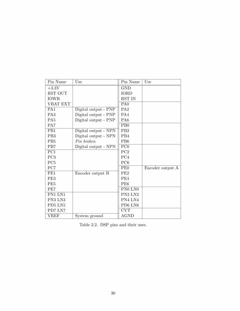
The DSP runs the control program provided in Appendix B, and communicates to the rest
of the system though a set of input and output pins. These I/O pins and their specific uses
are listed in Table 2.2. The DSPs specifications are provided in Appendix A, Figures A.5
and A.6.
2.6 Dump Load
In order to fully characterize the performance of a generator, it is necessary to vary both
its speed and the electrical load it powers. Once the motor is up and running, changing
the generator speed is a simple matter of changing the voltage input to the motor. To
vary the electrical load on the generator, it is necessary to develop a variable resistive load
compatible with the generators three phase output.
2.6.1 Resistors
The dump load is designed to utilize power resistors already available in RAEL. These
resistors can each dissipate up to 300 watts of power, and come in three resistances: 1.2 #,
8 #, and 15 #. By combining these resistances in di!erent series and parallel arrangements,
it is possible to create loads between 1.2 # and 46 # that can dissipate up to 1.5 kW.
29
Pin Name Use Pin Name Use+3.3V GNDRST OUT IORDIOWR RST INVBAT EXT PA0PA1 Digital output - PNP PA2PA3 Digital output - PNP PA4PA5 Digital output - PNP PA6PA7 PB0PB1 Digital output - NPN PB2PB3 Digital output - NPN PB4PB5 Pin broken PB6PB7 Digital output - NPN PC0PC1 PC2PC3 PC4PC5 PC6PC7 PE0 Encoder output APE1 Encoder output B PE2PE3 PE4PE5 PE6PE7 PN0 LN0PN1 LN1 PN2 LN2PN3 LN3 PN4 LN4PD5 LN5 PD6 LN6PD7 LN7 CVTVREF System ground AGND
Table 2.2. DSP pins and their uses.
30
2.6.2 Electrical System
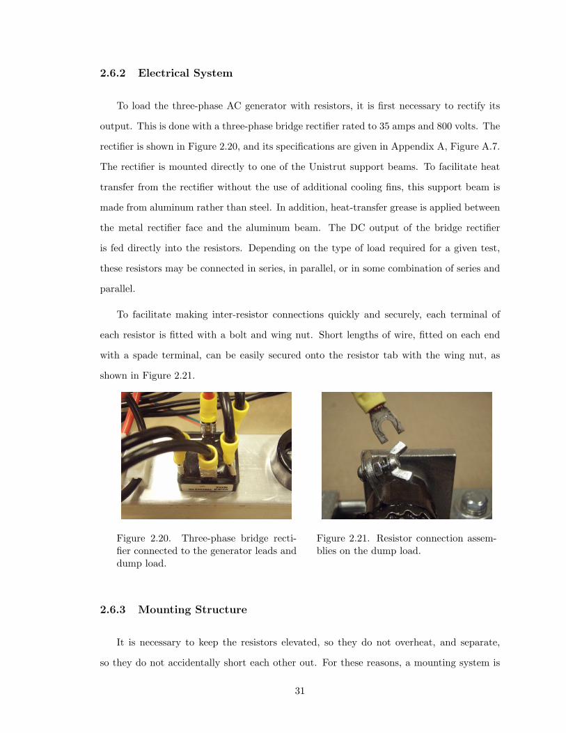
To load the three-phase AC generator with resistors, it is first necessary to rectify its
output. This is done with a three-phase bridge rectifier rated to 35 amps and 800 volts. The
rectifier is shown in Figure 2.20, and its specifications are given in Appendix A, Figure A.7.
The rectifier is mounted directly to one of the Unistrut support beams. To facilitate heat
transfer from the rectifier without the use of additional cooling fins, this support beam is
made from aluminum rather than steel. In addition, heat-transfer grease is applied between
the metal rectifier face and the aluminum beam. The DC output of the bridge rectifier
is fed directly into the resistors. Depending on the type of load required for a given test,
these resistors may be connected in series, in parallel, or in some combination of series and
parallel.
To facilitate making inter-resistor connections quickly and securely, each terminal of
each resistor is fitted with a bolt and wing nut. Short lengths of wire, fitted on each end
with a spade terminal, can be easily secured onto the resistor tab with the wing nut, as
shown in Figure 2.21.
Figure 2.20. Three-phase bridge recti-fier connected to the generator leads anddump load.
Figure 2.21. Resistor connection assem-blies on the dump load.
2.6.3 Mounting Structure
It is necessary to keep the resistors elevated, so they do not overheat, and separate,
so they do not accidentally short each other out. For these reasons, a mounting system is
31
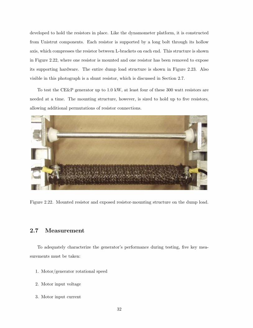
developed to hold the resistors in place. Like the dynamometer platform, it is constructed
from Unistrut components. Each resistor is supported by a long bolt through its hollow
axis, which compresses the resistor between L-brackets on each end. This structure is shown
in Figure 2.22, where one resistor is mounted and one resistor has been removed to expose
its supporting hardware. The entire dump load structure is shown in Figure 2.23. Also
visible in this photograph is a shunt resistor, which is discussed in Section 2.7.
To test the CE&P generator up to 1.0 kW, at least four of these 300 watt resistors are
needed at a time. The mounting structure, however, is sized to hold up to five resistors,
allowing additional permutations of resistor connections.
Figure 2.22. Mounted resistor and exposed resistor-mounting structure on the dump load.
2.7 Measurement
To adequately characterize the generator’s performance during testing, five key mea-
surements must be taken:
1. Motor/generator rotational speed
2. Motor input voltage
3. Motor input current
32
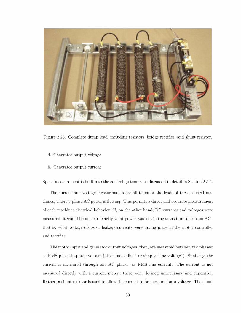
Figure 2.23. Complete dump load, including resistors, bridge rectifier, and shunt resistor.
4. Generator output voltage
5. Generator output current
Speed measurement is built into the control system, as is discussed in detail in Section 2.5.4.
The current and voltage measurements are all taken at the leads of the electrical ma-
chines, where 3-phase AC power is flowing. This permits a direct and accurate measurement
of each machines electrical behavior. If, on the other hand, DC currents and voltages were
measured, it would be unclear exactly what power was lost in the transition to or from AC–
that is, what voltage drops or leakage currents were taking place in the motor controller
and rectifier.
The motor input and generator output voltages, then, are measured between two phases:
as RMS phase-to-phase voltage (aka “line-to-line” or simply “line voltage”). Similarly, the
current is measured through one AC phase: as RMS line current. The current is not
measured directly with a current meter: these were deemed unnecessary and expensive.
Rather, a shunt resistor is used to allow the current to be measured as a voltage. The shunt
33
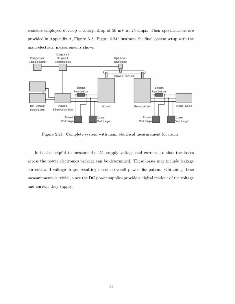
resistors employed develop a voltage drop of 50 mV at 25 amps. Their specifications are
provided in Appendix A, Figure A.8. Figure 2.24 illustrates the final system setup with the
main electrical measurements shown.
Figure 2.24. Complete system with main electrical measurement locations.
It is also helpful to measure the DC supply voltage and current, so that the losses
across the power electronics package can be determined. These losses may include leakage
currents and voltage drops, resulting in some overall power dissipation. Obtaining these
measurements is trivial, since the DC power supplies provide a digital readout of the voltage
and current they supply.
34
Chapter 3
Testing
The perception of electric shock can be di!erent depending on the voltage,duration, current, path taken, frequency, etc. Current entering the hand hasa threshold of perception of about 5 to 10 mA (milliampere) for DC and about1 to 10 mA for AC at 60 Hz.
– wikipedia
35

3.1 Overview
Once the dynamometer’s subsystems are complete and assembled, testing can begin.
The goals of this first round of testing are twofold:
1. Assess the performance of the dynamometer. Ensure that it works as designed, and
characterize its operation as a function of measured quantities.
2. Assess the performance of the CE&P generator.
Based on the analytical methods developed in Chapter 4, these two goals are performed
simultaneously, using the simplifying fact that the generator and motor are identical. Of
concern here is the problem of fulfilling these dual objectives within a very limited time-
frame. It is entirely possible that the dynamometer could not work as designed; it could,
say, fail at some current below the 30 amp design current. Such a failure would be a show-
stopper: testing could not continue without a functioning system, and diagnosing and fixing
a fault could take a considerable amount of time.
To address this concern, a testing sequence is chosen that begins by loading the system
as lightly as possible. By beginning with a high dump load resistance, both the electrical
currents and mechanical torque are minimized. As testing proceeds the dump load resistance
is decreased, and the system experiences higher currents and torques. This strategy has
two advantages. First, since currents and torques increase gradually, potential problems
like mechanical deflections, vibrations, overheating, or excess current draw can be identified
before they cause damage. Second, even if a system failure does occur, a set of data up
to the failure point will have been collected. This partial data set could help diagnose the
failure (or near-failure) and could even be su"cient to allow preliminary analysis of the
dynamometer and generator.
3.2 Test Plan
With this strategy in mind, the following test plan is developed:
36
1. Begin with no dump load resistors connected (open circuit: infinite resistance).
2. Begin with a DC supply voltage of 10V.
3. Collect system speed, input line voltage, input shunt voltage, output line voltage,
output shunt voltage, and DC supply current.
4. Increase DC supply voltage by 5V, and repeat data collection.
5. After the DC supply voltage reaches 50V, return to 10V and decrease dump load
resistance to the next increment.
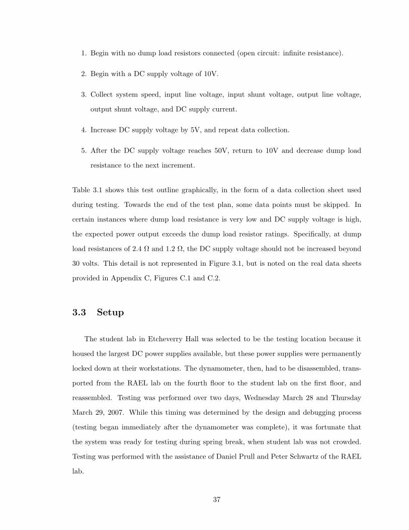
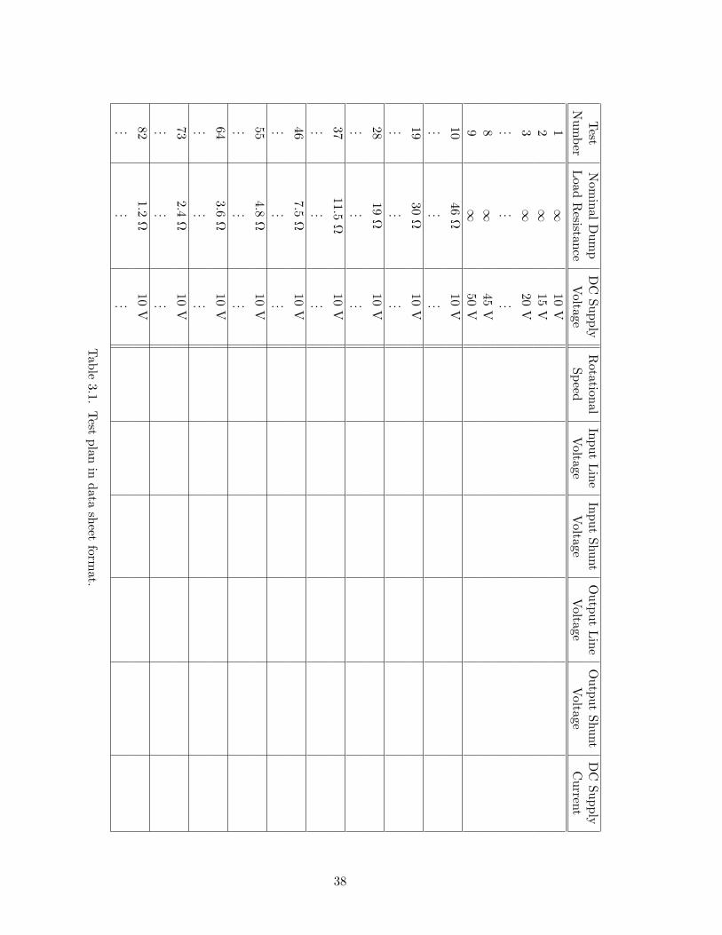
Table 3.1 shows this test outline graphically, in the form of a data collection sheet used
during testing. Towards the end of the test plan, some data points must be skipped. In
certain instances where dump load resistance is very low and DC supply voltage is high,
the expected power output exceeds the dump load resistor ratings. Specifically, at dump
load resistances of 2.4 # and 1.2 #, the DC supply voltage should not be increased beyond
30 volts. This detail is not represented in Figure 3.1, but is noted on the real data sheets
provided in Appendix C, Figures C.1 and C.2.
3.3 Setup
The student lab in Etcheverry Hall was selected to be the testing location because it
housed the largest DC power supplies available, but these power supplies were permanently
locked down at their workstations. The dynamometer, then, had to be disassembled, trans-
ported from the RAEL lab on the fourth floor to the student lab on the first floor, and
reassembled. Testing was performed over two days, Wednesday March 28 and Thursday
March 29, 2007. While this timing was determined by the design and debugging process
(testing began immediately after the dynamometer was complete), it was fortunate that
the system was ready for testing during spring break, when student lab was not crowded.
Testing was performed with the assistance of Daniel Prull and Peter Schwartz of the RAEL
lab.
37
TestN
ominalD
ump
DC
SupplyR
otationalInput
LineInput
ShuntO
utputLine
Output
ShuntD
CSupply
Num
berLoad
Resistance
Voltage
SpeedV
oltageV
oltageV
oltageV
oltageC
urrent1
#10
V2
#15
V3
#20
V...
......
8#
45V
9#
50V
1046
#10
V...
......
1930
#10
V...
......
2819
#10
V...
......
3711.5
#10
V...
......
467.5
#10
V...
......
554.8
#10
V...
......
643.6
#10
V...
......
732.4
#10
V...
......
821.2
#10
V...
......
Table3.1.
Testplan
indata
sheetform
at.
38
The dynamometer frame was slightly larger than the narrow desktops in the student
lab, but once secured down with clamps, was quite stable. Two power supplies were used
in series to supply the DC supply power. Each power supply had a rated output of 35 volts
and 25 amps, giving a total possible output of 70 volts and 25 amps. Because of the series
configuration, the DC current output could be read from either power supply, and the DC
voltage was obtained by adding the output voltages of each.
While relocating to the student lab was not ideal, it had the additional advantage of
providing an abundance of voltage meters. Each voltage output was connected to one
voltage meter, making data collection much easier than if one meter had been used to
sample every output.
3.4 Test Round 1
The first day of testing began well, and data at all voltage levels was obtained for the
first two dump load resistance values. However, as testing progressed and the dump load
resistances were decreased, two problems began to develop. First, the supply current began
to increase more quickly than expected, indicating that either (a) there was a considerable
amount of leakage current passing through the power electronics, or (b) something was
putting an extra load on the system, forcing the motor to draw more power. Second, a
“grinding” sound began to emanate from the encoder, which could be seen visibly bending
at its shaft. For fear of destroying the encoder, testing was immediately halted for the day.
Eventually, with the help of the student shop sta!, it was determined that the problem
lay in the positioning of the encoder. The encoder sprocket was incorrectly engaging the
taut side of the drive chain. As the dump load resistance decreased, the electrical machines
developed greater torque. This created more tension in the taut side of the chain, increasing
the force on the encoder sprocket. The encoder shaft was unable to handle this bending
force, causing the shaft to deflect and make the observed grinding sound. The extra loading
this grinding placed on the system may have also explained the increase in current drawn
by the system.
39

A solution proved rather simple: the encoder was simply repositioned to the slack side
of the chain. Luckily, the encoder was not damaged, and the system was up and running
once again. Data from this first day of testing was thrown out, to be repeated with the
improved test setup.
3.5 Test Round 2
The second day of testing proceeded much more smoothly, and the system performed
well enough to gather data at all planned resistance values. Another strange phenomenon
was observed, however: at low resistances and high voltages, a new grinding sound was
heard, but could not be located. The sound was accompanied by unsteady voltage readings.
It could be eliminated by resetting and restarting the dynamometer, but would eventually
return. But no cause was immediately evident–it seemed that the problem might be internal
to the electrical machines themselves–so once data was gathered at each resistance value,
testing was stopped and the test setup broken down.
The underlying problem was eventually discovered: at high torques, the generator’s
drive sprocket was actually slipping with respect to the generator shaft. This was able
happen because the generator sprocket was pulled counter-clockwise by the motor (as viewed
from above) while the generator tried to resist this motion, creating a clockwise torque. With
the torques arrayed in this manner, the nut holding the generator sprocket in place would
tend to loosen, gripping the sprocket less firmly. The motor sprocket, however, experienced
forces in the opposite directions, properly causing the nut holding its sprocket to tighten
as torques increased. The deep grinding sounds, then, were caused by the steel sprocket
moving against the generator shaft. This also produced a fine black dust that settled on
the generator, as the sprocket was slightly worn by the grinding action. The fact that the
system ran unsteadily could be due to the fact that the grinding was not perfectly constant,
but rather a cycle of sticking and slipping that became more intense as the nut loosened
further.
Unfortunately there was simply was not su"cient time to redesign the dynamometer
40
to address this problem. While a solution is absolutely necessary for future use of the
dynamometer, it was not immediately necessary. Even though the problem a!ected a
significant amount of data, enough valid data remained to begin preliminary analysis of the
dynamometer and generator.
3.6 Raw Data
The raw data obtained during the second day of testing is provided in Appendix C,
Figures C.1 and C.2. In these figures, data points shaded grey are those that are deemed
questionable (due to unsteady readings or other observations), and are not used in analysis
of the system. While the majority of the questionable data is due to the sprocket slippage
problem, it was also observed that low-voltage operation produced consistently unsteady
results. There are two possibilities for this unsteadiness: either the dynamometer does not
operate smoothly as slow speeds, or the voltage meters were unable to give a steady RMS
readings as slow electrical frequencies. In either case, this is not considered problematic.
The unsteady low-voltage data is discarded, and future tests should start at an input voltage
of 20 volts rather than 10 volts.
After purging all remotely questionable data points, 33 remain. They range over input
voltages of 20 to 50 volts, and dump loads from open circuit to 11.5 #. This is su"cient to
begin preliminary analysis of the dynamometer and the CE&P generator.
41

42
Chapter 4
Analysis
Heisenberg Something you’re always accusing me of. ‘If it works it works.’Never mind what it means.Bohr Of course I mind what it means.Heisenberg What it means in plain language.Bohr In plain language, yes.
– Michael FraynCopenhagen
43
4.1 Overview
Once testing has been performed, the resultant data is analyzed with two goals in mind:
assess the performance of the dynamometer, and assess the performance of the CE&P
generator. First, the entire dynamometer-generator system is addressed in Section 4.2.1. In
this section the overall energy flows within the system are characterized. This enables the
dynamometer’s characteristics to be quantified in Section 4.3. Finally, the CE&P machine
is assessed as a generator in Section 4.4.
4.2 Basic Analysis
4.2.1 Energy Balance
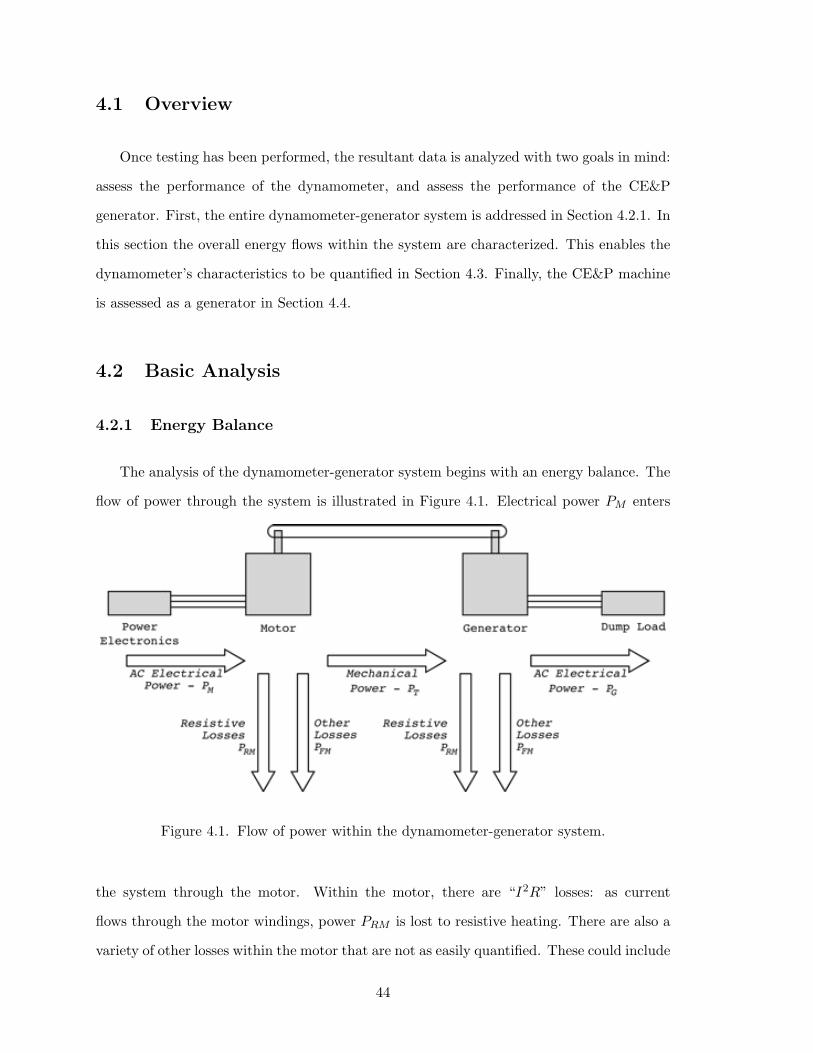
The analysis of the dynamometer-generator system begins with an energy balance. The
flow of power through the system is illustrated in Figure 4.1. Electrical power PM enters
Figure 4.1. Flow of power within the dynamometer-generator system.
the system through the motor. Within the motor, there are “I2R” losses: as current
flows through the motor windings, power PRM is lost to resistive heating. There are also a
variety of other losses within the motor that are not as easily quantified. These could include
44
viscous, Coulomb friction, eddy-current, or hysteresis losses, and are lumped together as
PFM . The remaining power PT is transmitted to the generator mechanically through the
drivetrain. The generator, like the motor, experiences resistive and miscellaneous losses PRG
and PFG. The remainder exits the generator as electrical power. Equation 4.1 represents
this energy balance mathematically.
PM = PRM + PFM + PT
= PRM + PFM + PRG + PFG + PG (4.1)
The voltage input to the motor, VLM , is measured as an RMS line-to-line voltage. The
voltage output of the generator is also an RMS line-to-line voltage, VLG. They are related
to the voltages over a single phase, VPM and VPG by equations 4.2 and 4.3.
VLM =$
3VPM (4.2)
VLG =$
3VPG (4.3)
The RMS line current to the motor, ILM , and from the generator, ILG, are also measured.
The current through one phase is the same as the line current.
ILM = IPM = IM (4.4)
ILG = IPG = IG (4.5)
The power input to the motor is the product of voltage and current over one phase times
the number of phases. The power output of the generator is defined in the same way.
PM = 3VPMIM =$
3VLMIM (4.6)
PG = 3VPGIG =$
3VLGIG (4.7)
Before testing, the resistance of each motor and generator phase is measured with a multi-
meter. Since the phases are balanced and the electrical machines are identical, the resistance
45
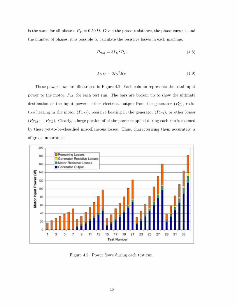
is the same for all phases: RP = 0.50 #. Given the phase resistance, the phase current, and
the number of phases, it is possible to calculate the resistive losses in each machine.
PRM = 3IM2RP (4.8)
PGM = 3IG2RP (4.9)
These power flows are illustrated in Figure 4.2. Each column represents the total input
power to the motor, PM , for each test run. The bars are broken up to show the ultimate
destination of the input power: either electrical output from the generator (PG), resis-
tive heating in the motor (PRM ), resistive heating in the generator (PRG), or other losses
(PFM + PFG). Clearly, a large portion of of the power supplied during each run is claimed
by these yet-to-be-classified miscellaneous losses. Thus, characterizing them accurately is
of great importance.
Figure 4.2. Power flows during each test run.
46
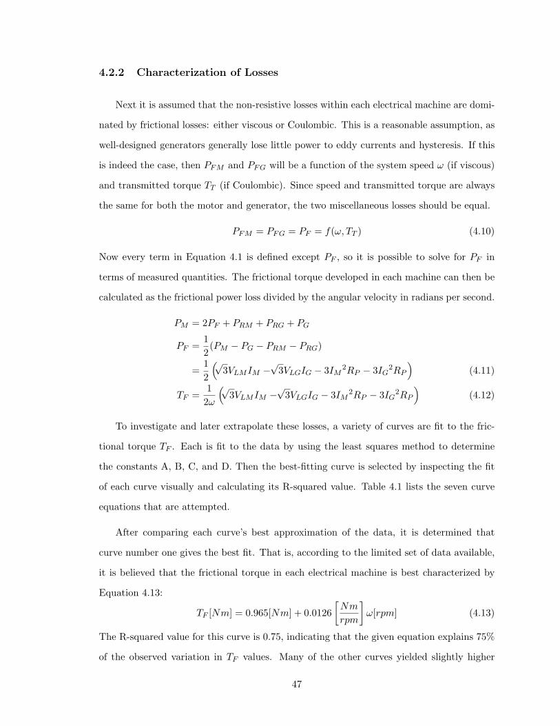
4.2.2 Characterization of Losses
Next it is assumed that the non-resistive losses within each electrical machine are domi-
nated by frictional losses: either viscous or Coulombic. This is a reasonable assumption, as
well-designed generators generally lose little power to eddy currents and hysteresis. If this
is indeed the case, then PFM and PFG will be a function of the system speed ! (if viscous)
and transmitted torque TT (if Coulombic). Since speed and transmitted torque are always
the same for both the motor and generator, the two miscellaneous losses should be equal.
PFM = PFG = PF = f(!, TT ) (4.10)
Now every term in Equation 4.1 is defined except PF , so it is possible to solve for PF in
terms of measured quantities. The frictional torque developed in each machine can then be
calculated as the frictional power loss divided by the angular velocity in radians per second.
PM = 2PF + PRM + PRG + PG
PF =12(PM " PG " PRM " PRG)
=12
!$3VLMIM "
$3VLGIG " 3IM
2RP " 3IG2RP
"(4.11)
TF =12!
!$3VLMIM "
$3VLGIG " 3IM
2RP " 3IG2RP
"(4.12)
To investigate and later extrapolate these losses, a variety of curves are fit to the fric-
tional torque TF . Each is fit to the data by using the least squares method to determine
the constants A, B, C, and D. Then the best-fitting curve is selected by inspecting the fit
of each curve visually and calculating its R-squared value. Table 4.1 lists the seven curve
equations that are attempted.
After comparing each curve’s best approximation of the data, it is determined that
curve number one gives the best fit. That is, according to the limited set of data available,
it is believed that the frictional torque in each electrical machine is best characterized by
Equation 4.13:
TF [Nm] = 0.965[Nm] + 0.0126#
Nm
rpm
$![rpm] (4.13)
The R-squared value for this curve is 0.75, indicating that the given equation explains 75%
of the observed variation in TF values. Many of the other curves yielded slightly higher
47
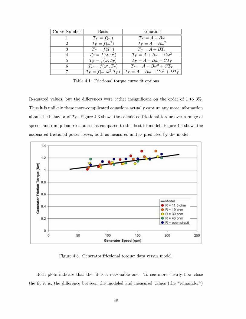
Curve Number Basis Equation1 TF = f(!) TF = A + B!2 TF = f(!2) TF = A + B!2
3 TF = f(TT ) TF = A + BTT
4 TF = f(!,!2) TF = A + B! + C!2
5 TF = f(!, TT ) TF = A + B! + CTT
6 TF = f(!2, TT ) TF = A + B!2 + CTT
7 TF = f(!, !2, TT ) TF = A + B! + C!2 + DTT
Table 4.1. Frictional torque curve fit options
R-squared values, but the di!erences were rather insignificant–on the order of 1 to 3%.
Thus it is unlikely these more-complicated equations actually capture any more information
about the behavior of TF . Figure 4.3 shows the calculated frictional torque over a range of
speeds and dump load resistances as compared to this best-fit model. Figure 4.4 shows the
associated frictional power losses, both as measured and as predicted by the model.
Figure 4.3. Generator frictional torque; data versus model.
Both plots indicate that the fit is a reasonable one. To see more clearly how close
the fit it is, the di!erence between the modeled and measured values (the “remainder”)
48
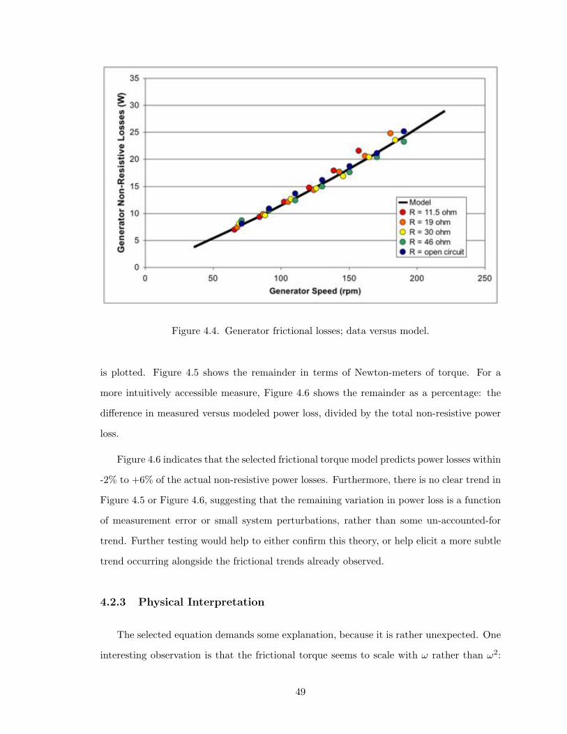
Figure 4.4. Generator frictional losses; data versus model.
is plotted. Figure 4.5 shows the remainder in terms of Newton-meters of torque. For a
more intuitively accessible measure, Figure 4.6 shows the remainder as a percentage: the
di!erence in measured versus modeled power loss, divided by the total non-resistive power
loss.
Figure 4.6 indicates that the selected frictional torque model predicts power losses within
-2% to +6% of the actual non-resistive power losses. Furthermore, there is no clear trend in
Figure 4.5 or Figure 4.6, suggesting that the remaining variation in power loss is a function
of measurement error or small system perturbations, rather than some un-accounted-for
trend. Further testing would help to either confirm this theory, or help elicit a more subtle
trend occurring alongside the frictional trends already observed.
4.2.3 Physical Interpretation
The selected equation demands some explanation, because it is rather unexpected. One
interesting observation is that the frictional torque seems to scale with ! rather than !2:
49
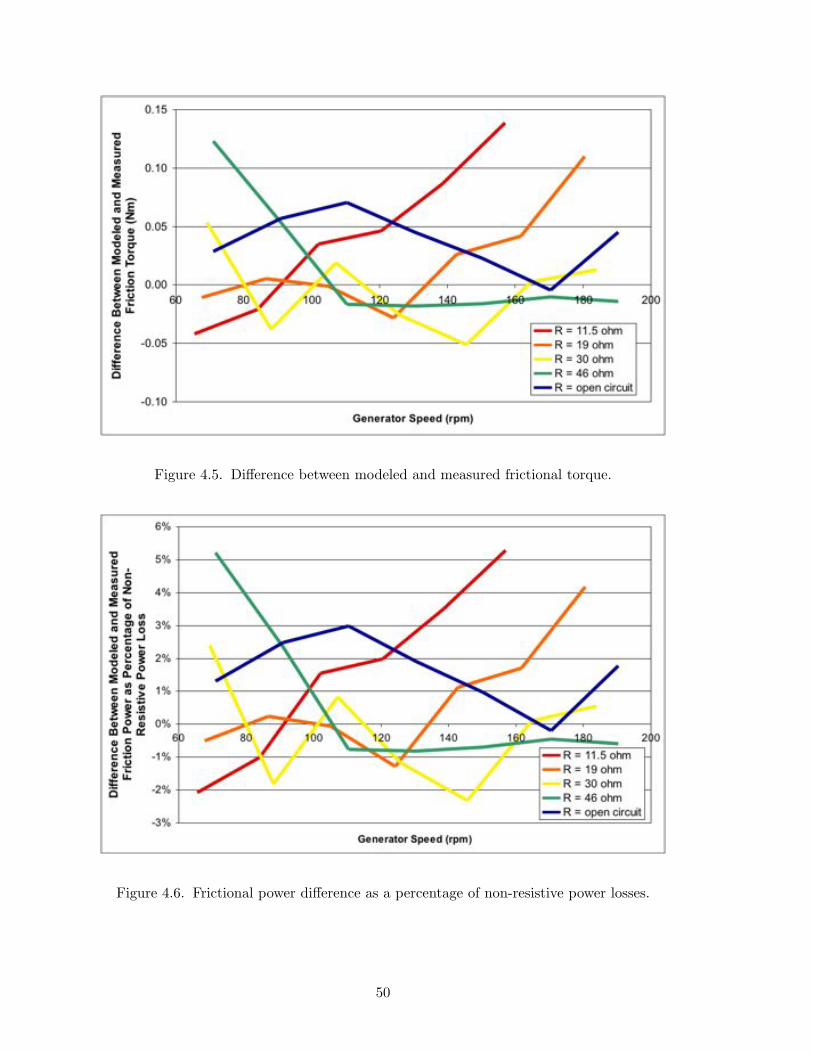
Figure 4.5. Di!erence between modeled and measured frictional torque.
Figure 4.6. Frictional power di!erence as a percentage of non-resistive power losses.
50
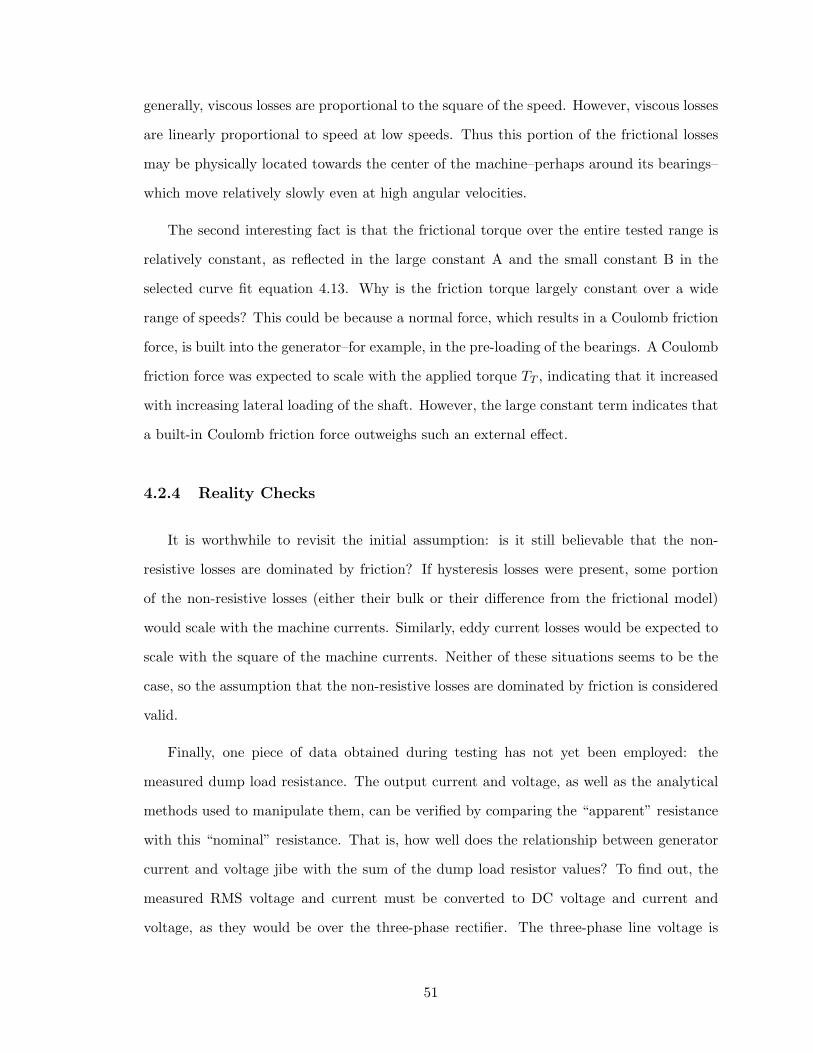
generally, viscous losses are proportional to the square of the speed. However, viscous losses
are linearly proportional to speed at low speeds. Thus this portion of the frictional losses
may be physically located towards the center of the machine–perhaps around its bearings–
which move relatively slowly even at high angular velocities.
The second interesting fact is that the frictional torque over the entire tested range is
relatively constant, as reflected in the large constant A and the small constant B in the
selected curve fit equation 4.13. Why is the friction torque largely constant over a wide
range of speeds? This could be because a normal force, which results in a Coulomb friction
force, is built into the generator–for example, in the pre-loading of the bearings. A Coulomb
friction force was expected to scale with the applied torque TT , indicating that it increased
with increasing lateral loading of the shaft. However, the large constant term indicates that
a built-in Coulomb friction force outweighs such an external e!ect.
4.2.4 Reality Checks
It is worthwhile to revisit the initial assumption: is it still believable that the non-
resistive losses are dominated by friction? If hysteresis losses were present, some portion
of the non-resistive losses (either their bulk or their di!erence from the frictional model)
would scale with the machine currents. Similarly, eddy current losses would be expected to
scale with the square of the machine currents. Neither of these situations seems to be the
case, so the assumption that the non-resistive losses are dominated by friction is considered
valid.
Finally, one piece of data obtained during testing has not yet been employed: the
measured dump load resistance. The output current and voltage, as well as the analytical
methods used to manipulate them, can be verified by comparing the “apparent” resistance
with this “nominal” resistance. That is, how well does the relationship between generator
current and voltage jibe with the sum of the dump load resistor values? To find out, the
measured RMS voltage and current must be converted to DC voltage and current and
voltage, as they would be over the three-phase rectifier. The three-phase line voltage is
51
related to the DC output voltage by Equation 4.14, where VB is the voltage drop across the
bridge rectifier: about 1.3 volts for a silicon rectifier operating in this current range.
VDC =3$
2"
VLG " VB (4.14)
Next, the DC output current must be determined from the RMS phase current. The current
output of each phase is a form of square wave, determined by the sequence in which the
rectifier diodes conduct. The phase current is Imax for 120!, zero for 60!, "Imax for 120!,
and again zero for 60!. These square waves nest together such that Imax = IDC : the DC
current is equal to the maximum phase current. Therefore to determine IDC , it is necessary
to determine Imax as a function of IRMS given the shape of the square wave. Using the
definition of the RMS (root-mean-square) value,
IDC = Imax =
%360!
(1)2120! + ("1)2120! + 02120!IRMS =
&32IRMS (4.15)
Now the apparent resistance can be calculated.
Rapparent =VDC
IDC=
2$
3"
'VLG "
(2/3VB
IRMS
)(4.16)
Calculated as such, the apparent resistances are very close to the measured resistances:
within +/- 1 #, or +/- 4%. The calculated resistances vary slightly, but nearly always
increase from one test to the next. This is to be expected: as testing continues the resistors
heat up, causing their resistance values to increase slightly. This similarity between apparent
and nominal resistance values is very encouraging.
4.3 Dynamometer Results
Having quantified the various power flows within the dynamometer-generator sys-
tem and characterized the remaining power loss, it is possible to begin analyzing the
dynamometer–that is, the motor and the power electronics that drive it. The primary
goal of this analysis is to determine the driving torque produced by the motor, because
the assessment of the CE&P generator depends on it. Furthermore, a torque equation
will enable the dynamometer to be employed usefully in the future: the dynamometer’s
52
applied torque will be determined from experimental data and used to asses any genera-
tor’s response to such torque. A secondary goal of the dynamometer analysis is to quantify
the losses across the power electronics package. While it is not necessary that the power
electronics be e"cient per se, it is worthwhile to ensure that they do not experience large
voltage drops, leakage currents, or power losses–any of which could signal a potentially
damaging problem within the power electronics package.
4.3.1 Torque Output
Applying equation 4.1 over the motor alone, the mechanical power transmitted by the
motor is determined as a function of the motor’s input power, resistive power losses, and
frictional power losses.
PT = PM " PRM " PF (4.17)
The transmitted torque, then, is determined by dividing the transmitted power by the
angular velocity. The expression is then simplified and put in terms of measured quantities
alone.
TT =1!
[PM " PRM " PF ]
=1!
[PM " PRM ]" TF
=1!
*$3VLMIM " IM
2RP
+"A + B! (4.18)
Table 4.2 shows the final dynamometer torque equation and all the information required to
use it.
4.3.2 Power Electronics Performance
To asses the leakage current, voltage drop, and power loss within the power electronics
package, its DC electrical input is compared to its AC output (the AC input to the motor).
The DC input voltage, VIN"DC is shown on the power supply displays. To enable a direct
comparison, the RMS motor line voltage is converted to a DC voltage. This is done exactly
as it was in Section 4.2.4, where the RMS output of the generator was converted to DC
53
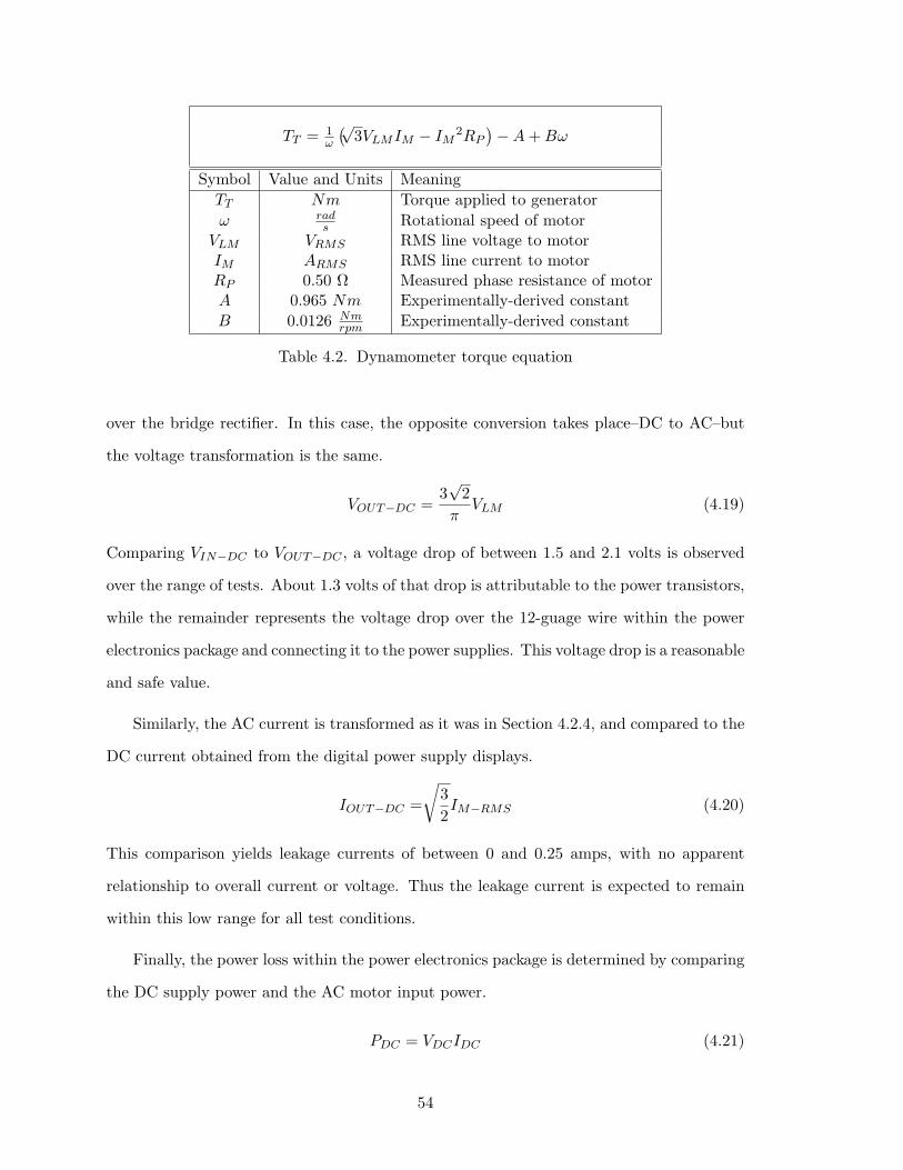
TT = 1!
,$3VLMIM " IM
2RP-"A + B!
Symbol Value and Units MeaningTT Nm Torque applied to generator! rad
s Rotational speed of motorVLM VRMS RMS line voltage to motorIM ARMS RMS line current to motorRP 0.50 # Measured phase resistance of motorA 0.965 Nm Experimentally-derived constantB 0.0126 Nm
rpm Experimentally-derived constant
Table 4.2. Dynamometer torque equation
over the bridge rectifier. In this case, the opposite conversion takes place–DC to AC–but
the voltage transformation is the same.
VOUT"DC =3$
2"
VLM (4.19)
Comparing VIN"DC to VOUT"DC , a voltage drop of between 1.5 and 2.1 volts is observed
over the range of tests. About 1.3 volts of that drop is attributable to the power transistors,
while the remainder represents the voltage drop over the 12-guage wire within the power
electronics package and connecting it to the power supplies. This voltage drop is a reasonable
and safe value.
Similarly, the AC current is transformed as it was in Section 4.2.4, and compared to the
DC current obtained from the digital power supply displays.
IOUT"DC =&
32IM"RMS (4.20)
This comparison yields leakage currents of between 0 and 0.25 amps, with no apparent
relationship to overall current or voltage. Thus the leakage current is expected to remain
within this low range for all test conditions.
Finally, the power loss within the power electronics package is determined by comparing
the DC supply power and the AC motor input power.
PDC = VDCIDC (4.21)
54
PAC =$
3VLMIM (4.22)
The power loss is found to range between 0.7 and 11 watts, giving an e"ciency of 80% to
99%. This amount of power dissipation is low enough that is not cause for concern–11 watts
should be easily dissipated by the transistors and other components. The power loss does
not seem to track well with overall current or voltage, however, so it is di"cult to predict
how much power the package will have to dissipate at higher currents. Thus, testing at
higher currents should proceed with caution.
4.4 Generator Results
4.4.1 Overview
At last, using the results of the overall and dynamometer analyses, the generator’s
properties can be evaluated. One way to evaluate a generator is to simply run it at the
points of interest and measure what happens. If the generator is expected to operate at
speeds (!1, !2, ..., !n) and load resistances (R1, R2, ..., Rn), it may be possible to run
tests at each of those specific combinations. To predict the behavior of the generator in
situations between these discrete data points, interpolation might give adequate results.
However, a more powerful tactic would be to develop a model of the generator. In
this case, data from dynamometer testing is used to inform and check the model. Such a
technique should give more accurate results than simply interpolating between data points.
Furthermore, modeling is crucial when the data gathered does not span the generator’s en-
tire potential range of operation–which, unfortunately, was the case with the first round of
CE&P generator testing. The analysis of the CE&P generator (or any other future gener-
ator) proceeds as follows: first, the generator’s motor constants are derived from test data.
Second, the energy methods used previously are employed once again to model the genera-
tor’s behavior based on only measured quantities, its speed, and its derived motor constant.
55
The resultant model is then checked against the data gathered during dynamometer testing.
Lastly, the model is used to assess the generator’s claimed specifications.
4.4.2 Motor Constant
The motor constant has two incarnations: the voltage constant relates the generator’s
open-circuit voltage to its speed, while the torque constant relates the back torque of the
generator to the current that flows through it. Under certain conditions both constants
should be equal, so as a check both constants are evaluated and compared. First, the
voltage constant is determined. This is done by fitting a line to the generator’s open circuit
voltage-versus-speed data. The slope of this line is the voltage constant, presented in three
di!erent units.
Kv = 0.184VRMS line"to"line
rpm(4.23)
= 1.76VRMS line"to"line
rad/s(4.24)
= 1.01VRMS line"to"neut
rad/s(4.25)
Next, the torque constant is determined: in theory, it should be equal to the value of Kv
given in Equation 4.25. The e!ective torque constant can be found at each data point.
These values vary only very slightly, and are averaged to give an overall torque constant.
Kt =TT " TF
3IG(4.26)
Kt = 1.02Nm
ARMS total(4.27)
Indeed, the Kv and Kt values match up extremely closely–they di!er by only 0.6%.
4.4.3 Generator Modeling
Current Equation
Now it is possible to develop relations for the generator current, voltage, torque, e"-
ciency, and power output, given any generator speed and dump load resistance. The analysis
56
begins with an energy balance over the generator, which is expressed in terms of torques
by dividing through by the rotational speed. Next, the torque terms are combined and the
power terms are expanded.
PT = PG + PRG + PF (4.28)
TT =PG + PRG
!+ TF (4.29)
TT " TF =$
3IGVLG + 3IG2RP
!(4.30)
This equation contains four variables: the applied torque TT , the phase current IG, the line
voltage VLG, and the rotational speed !. Since the first three of these variables must be
isolated and related to ! and the dump load resistance alone, two more relations are needed
to unravel Equation 4.30. The first is torque constant identity of Equation 4.27. Plugging
this in puts the torque variables in terms of the phase current.
3KtIG =$
3IGVLG + 3IG2RP
!(4.31)
3Kt! =$
3VLG + 3IGRP (4.32)
The line voltage can also be related to the phase current. First, Ohm’s law is used to relate
the DC current and voltage over the dump load resistance RD. The DC current and voltage
are then replaced by their AC equivalents, as defined in Section 4.2.4.
VDC = IDCRD (4.33)
3$
2"
VLG " VD =&
32IGRD (4.34)
VLG ="
2$
3IGRD +
"
3$
2VD (4.35)
Now VLG is plugged into Equation 4.32, so that the phase current alone is related to the
two variables: rotational speed and dump load resistance. The equation is solved for the
phase current IG, and constitutes the first useful equation of the generator model.
3Kt! =$
3#
"
2$
3IGRD +
"
3$
2VD
$+ 3IGRP (4.36)
3Kt! ""$6VD = IG
!"
2RD + 3RP
"(4.37)
IG =3Kt! " "#
6VD
"2 RD + 3RP
(4.38)
57
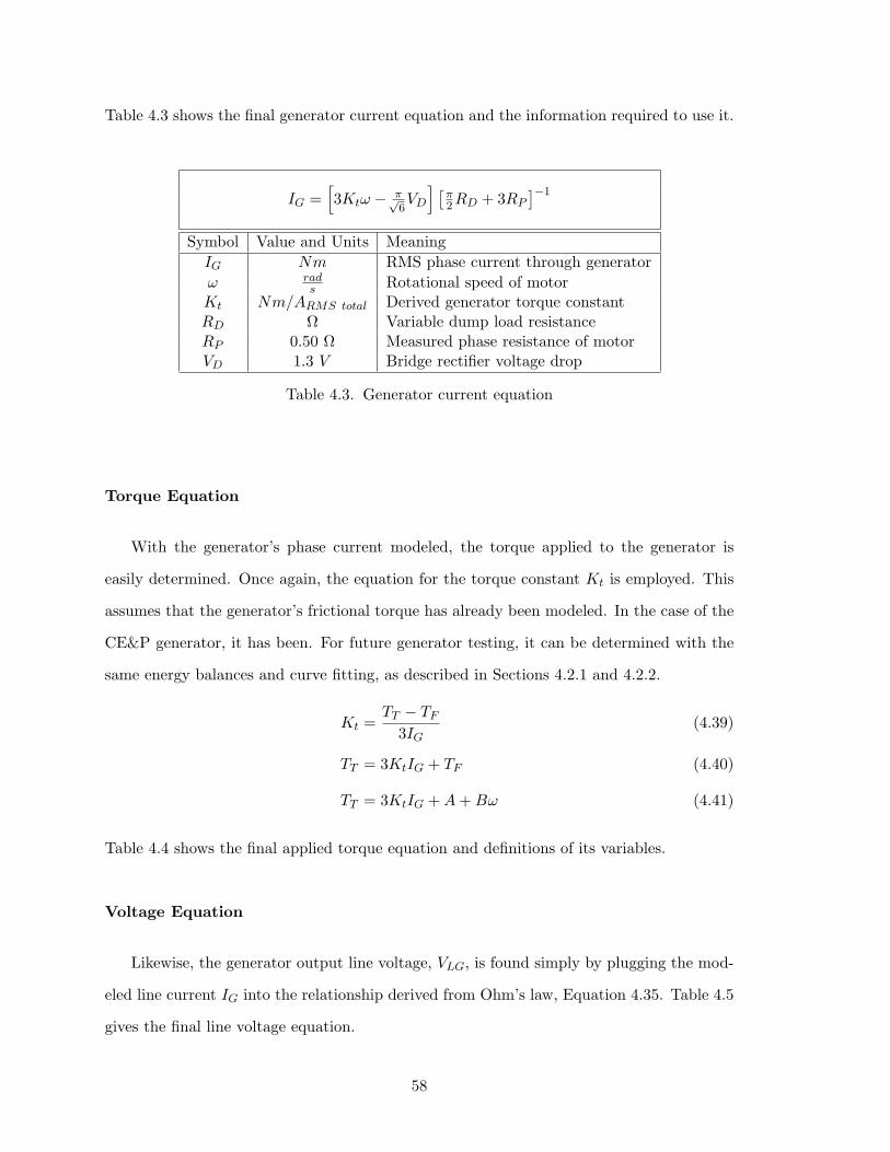
Table 4.3 shows the final generator current equation and the information required to use it.
IG =*3Kt! " "#
6VD
+ ."2 RD + 3RP
/"1
Symbol Value and Units MeaningIG Nm RMS phase current through generator! rad
s Rotational speed of motorKt Nm/ARMS total Derived generator torque constantRD # Variable dump load resistanceRP 0.50 # Measured phase resistance of motorVD 1.3 V Bridge rectifier voltage drop
Table 4.3. Generator current equation
Torque Equation
With the generator’s phase current modeled, the torque applied to the generator is
easily determined. Once again, the equation for the torque constant Kt is employed. This
assumes that the generator’s frictional torque has already been modeled. In the case of the
CE&P generator, it has been. For future generator testing, it can be determined with the
same energy balances and curve fitting, as described in Sections 4.2.1 and 4.2.2.
Kt =TT " TF
3IG(4.39)
TT = 3KtIG + TF (4.40)
TT = 3KtIG + A + B! (4.41)
Table 4.4 shows the final applied torque equation and definitions of its variables.
Voltage Equation
Likewise, the generator output line voltage, VLG, is found simply by plugging the mod-
eled line current IG into the relationship derived from Ohm’s law, Equation 4.35. Table 4.5
gives the final line voltage equation.
58
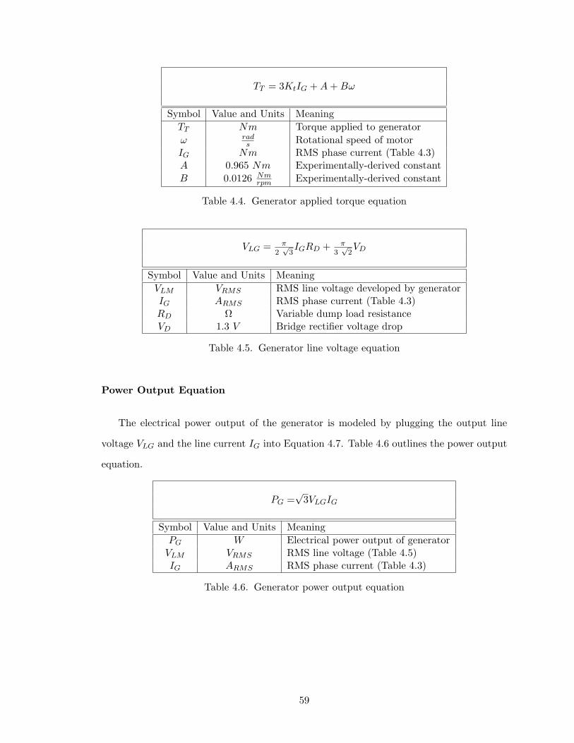
TT = 3KtIG + A + B!
Symbol Value and Units MeaningTT Nm Torque applied to generator! rad
s Rotational speed of motorIG Nm RMS phase current (Table 4.3)A 0.965 Nm Experimentally-derived constantB 0.0126 Nm
rpm Experimentally-derived constant
Table 4.4. Generator applied torque equation
VLG = "2#
3IGRD + "
3#
2VD
Symbol Value and Units MeaningVLM VRMS RMS line voltage developed by generatorIG ARMS RMS phase current (Table 4.3)RD # Variable dump load resistanceVD 1.3 V Bridge rectifier voltage drop
Table 4.5. Generator line voltage equation
Power Output Equation
The electrical power output of the generator is modeled by plugging the output line
voltage VLG and the line current IG into Equation 4.7. Table 4.6 outlines the power output
equation.
PG =$
3VLGIG
Symbol Value and Units MeaningPG W Electrical power output of generator
VLM VRMS RMS line voltage (Table 4.5)IG ARMS RMS phase current (Table 4.3)
Table 4.6. Generator power output equation
59
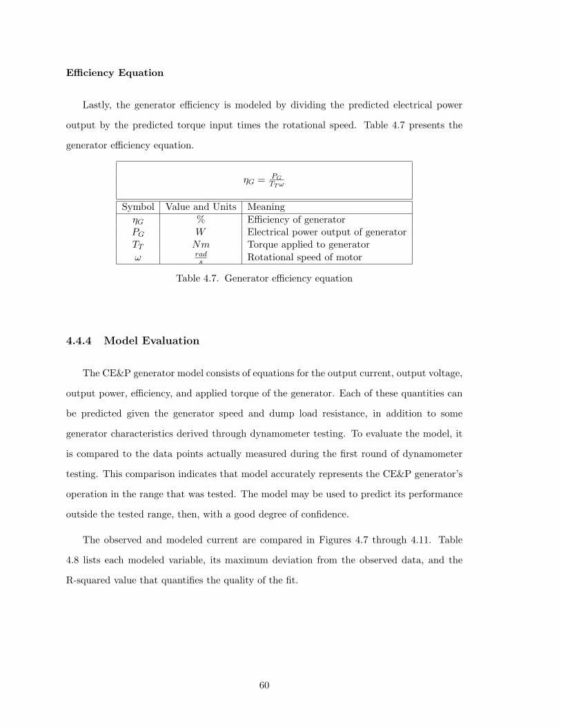
E!ciency Equation
Lastly, the generator e"ciency is modeled by dividing the predicted electrical power
output by the predicted torque input times the rotational speed. Table 4.7 presents the
generator e"ciency equation.
#G = PGTT !
Symbol Value and Units Meaning#G % E"ciency of generatorPG W Electrical power output of generatorTT Nm Torque applied to generator! rad
s Rotational speed of motor
Table 4.7. Generator e"ciency equation
4.4.4 Model Evaluation
The CE&P generator model consists of equations for the output current, output voltage,
output power, e"ciency, and applied torque of the generator. Each of these quantities can
be predicted given the generator speed and dump load resistance, in addition to some
generator characteristics derived through dynamometer testing. To evaluate the model, it
is compared to the data points actually measured during the first round of dynamometer
testing. This comparison indicates that model accurately represents the CE&P generator’s
operation in the range that was tested. The model may be used to predict its performance
outside the tested range, then, with a good degree of confidence.
The observed and modeled current are compared in Figures 4.7 through 4.11. Table
4.8 lists each modeled variable, its maximum deviation from the observed data, and the
R-squared value that quantifies the quality of the fit.
60
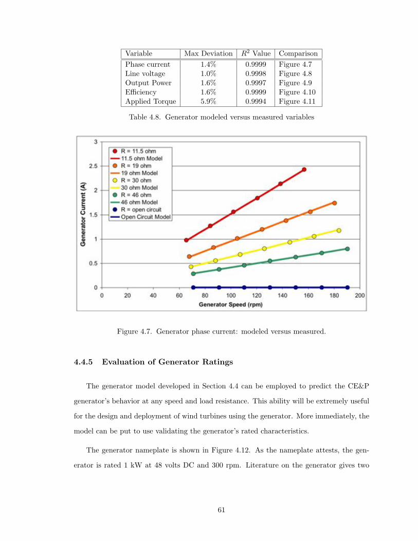
Variable Max Deviation R2 Value ComparisonPhase current 1.4% 0.9999 Figure 4.7Line voltage 1.0% 0.9998 Figure 4.8Output Power 1.6% 0.9997 Figure 4.9E"ciency 1.6% 0.9999 Figure 4.10Applied Torque 5.9% 0.9994 Figure 4.11
Table 4.8. Generator modeled versus measured variables
Figure 4.7. Generator phase current: modeled versus measured.
4.4.5 Evaluation of Generator Ratings
The generator model developed in Section 4.4 can be employed to predict the CE&P
generator’s behavior at any speed and load resistance. This ability will be extremely useful
for the design and deployment of wind turbines using the generator. More immediately, the
model can be put to use validating the generator’s rated characteristics.
The generator nameplate is shown in Figure 4.12. As the nameplate attests, the gen-
erator is rated 1 kW at 48 volts DC and 300 rpm. Literature on the generator gives two
61
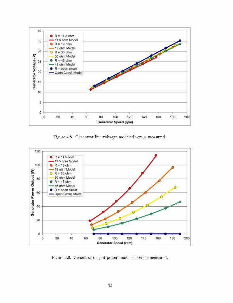
Figure 4.8. Generator line voltage: modeled versus measured.
Figure 4.9. Generator output power: modeled versus measured.
62
Figure 4.10. Generator e"ciency: modeled versus measured.
Figure 4.11. Generator applied torque: modeled versus measured.
63
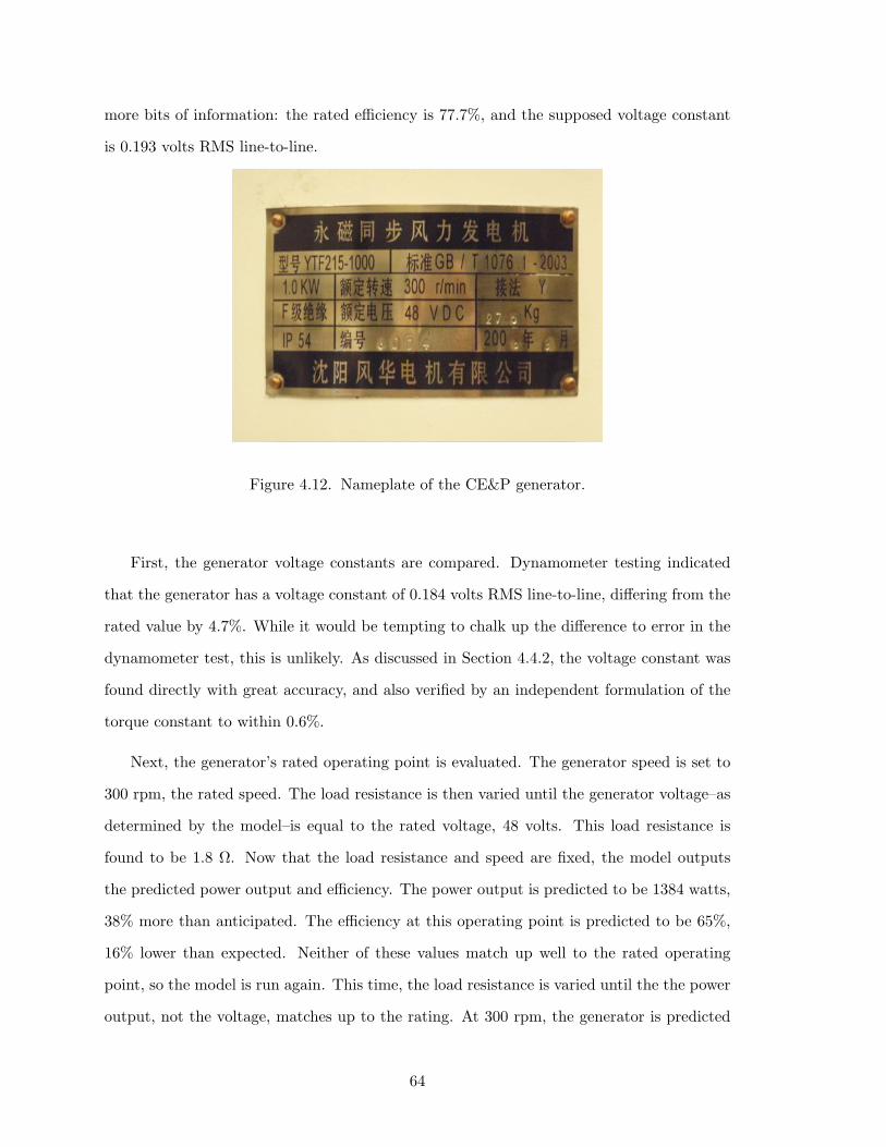
more bits of information: the rated e"ciency is 77.7%, and the supposed voltage constant
is 0.193 volts RMS line-to-line.
Figure 4.12. Nameplate of the CE&P generator.
First, the generator voltage constants are compared. Dynamometer testing indicated
that the generator has a voltage constant of 0.184 volts RMS line-to-line, di!ering from the
rated value by 4.7%. While it would be tempting to chalk up the di!erence to error in the
dynamometer test, this is unlikely. As discussed in Section 4.4.2, the voltage constant was
found directly with great accuracy, and also verified by an independent formulation of the
torque constant to within 0.6%.
Next, the generator’s rated operating point is evaluated. The generator speed is set to
300 rpm, the rated speed. The load resistance is then varied until the generator voltage–as
determined by the model–is equal to the rated voltage, 48 volts. This load resistance is
found to be 1.8 #. Now that the load resistance and speed are fixed, the model outputs
the predicted power output and e"ciency. The power output is predicted to be 1384 watts,
38% more than anticipated. The e"ciency at this operating point is predicted to be 65%,
16% lower than expected. Neither of these values match up well to the rated operating
point, so the model is run again. This time, the load resistance is varied until the the power
output, not the voltage, matches up to the rating. At 300 rpm, the generator is predicted
64
to output 1000 watts when the load resistance is 3.6 #. At this operating point the voltage
is expected to be 58 volts–21% greater than expected. The e"ciency, however, is predicted
to be 77.0%, which matches up quite well with the rated 77.7% e"ciency.
Given these results, it is hard to assess exactly how much the model and the generator
ratings di!er, because it is unclear what specific operating points should be compared. In
any case, the model predicts behavior quite di!erent from that indicated by the machine’s
nominal ratings. There are three possibilities for this significant discrepancy:
1. The model may not be valid over the generator’s entire range of operation. At higher
torques and currents, the generator may exhibit behavior not observed during the first
round of testing.
2. The generators obtained by CE&P may not behave consistently. That is, each indi-
vidual electrical machine may exhibit di!erent qualities, due to manufacturing impre-
cision or lack of quality control.
3. The data provided by the generator manufacturer could be incorrect.
To determine what is truly taking place, it is crucial to retest the CE&P generator at
higher torques and currents, as was originally intended. This will either validate the model,
or inform a more accurate model. It would also be helpful to swap the two electrical
machines: use the generator as the dynamometer motor, and test the motor as a generator.
This would help address item number 2, and ensure that each machine behaves just like its
twin.
Lastly, the generator’s maximum e"ciency is evaluated, as predicted by the model.
Limiting the generator speed to 450 rpm, or 50% greater than its rated speed, the maximum
e"ciency is found to be 86% at 450 rpm and 13 #. At this operating point, the power output
is 873 watts.
65

66
Chapter 5
Summary and Conclusions
This matter is a pot of sweet potatoes.The words of all men point in one direction: agreement.
– Zulu proverb
67
5.1 Summary
The Renewable and Appropriate Energy Laboratory was contracted by California En-
ergy and Power to test a 1 kW permanent magnet generator for use in small, vertical axis
wind turbines. To enable testing of the generator, as well as to facilitate accurate analysis of
the test data, a driving dynamometer was developed using a second identical generator. The
dynamometer was comprised of several subsystems. A custom power electronics package,
optical encoder, and digital signal processor allowed one generator be driven as a motor,
providing the dynamometer’s motive force. A chain drive transferred mechanical power
from the motor to the generator, which was electrically loaded with a variable-resistance
dump load.
Testing was performed over two days. While an unresolved sprocket-mounting problem
prohibited testing their full range operation, enough data was collected to permit prelimi-
nary analysis of both the dynamometer and the generator. Analysis began by determining
the machines’ motor constants, as well as characterizing their non-resistive power losses.
With this information, the dynamometer’s torque output was determined as a function of
measured quantities. Then the generator itself was evaluated: using test results and genera-
tor theory, a model of the generator’s performance was developed. The model was found to
correlate extremely well to measured data points, and was used to evaluate the generator’s
manufacturer-specified ratings.
5.2 Conclusions
Through the process of designing, fabricating, and using the driving dynamometer,
several major conclusions have been reached.
68
Dynamometer
1. The dynamometer is a promising tool for testing small wind turbine generators. With
some improvements to the drivetrain, it should be able to test generators up to a
maximum of 240 rpm, 800 volts DC, 35 amps, 1 kW, and 40 Nm of applied torque.
2. The dynamometer should be run with a DC voltage input of 20 volts and above. This
will allow the test operator to bypass the range of unsteady operation observed below
20 volts.
CE&P Generator
1. The California Energy and Power 1 kW permanent magnet generator can be accu-
rately modeled in the low-power range that was tested. While it must be verified
through testing, the model is expected to hold up at higher power levels.
2. The CE&P generator experiences non-resistive power losses from what can be repre-
sented as a frictional torque. The frictional torque is approximated as the sum of a
constant value and a term proportional to the generator speed. This characterization
of the generator’s non-resistive power losses forms the basis of the generator model.
3. The model suggests that the CE&P generator’s motor constant and operating point
ratings are inaccurate, or vary considerably between supposedly-identical machines.
Again, this claim must be verified by testing at higher torque, current, and power
levels.
5.3 Future Work
Through preliminary testing and analysis, the dynamometer has proven that it can
function e!ectively and produce high-quality results. Further work is needed, however, to
complete the analysis of the CE&P generator, and enable the testing of other generators in
the future.
69
First and foremost, the problem outlined in Section 3.5 must be addressed: the chain
drive or generator shaft-to-sprocket connection must be redesigned, so that the connection
does not naturally loosen at high torques. This will enable the dynamometer to run tests
in the high torque, high current, and high power regime it was designed for. Once that
redesign takes place, the CE&P generator can be retested through a larger range of oper-
ating conditions. Retesting will serve as a check on the conclusions developed here: does
the generator actually perform as predicted by the model? Retesting should also involve
swapping the two CE&P generators, so each is run as both a motor and generator. By
comparing the results from two such tests, the consistency of individual generator units
produced by this manufacturer can be evaluated.
Beyond testing the CE&P generator, the dynamometer setup could use some improve-
ments if it is to continue testing generators for the RAEL laboratory. More than anything,
the dynamometer needs a home–specifically, a home with an adequately-sized DC power
supply. If it must be shipped to the student lab in Etcheverry for every test, it is unlikely
that the dynamometer will be used. Since RAEL is relocating to the Richmond Field Sta-
tion, this will may necessitate the purchase of a power supply for the lab. In the same
vein, at least one voltage meter should be obtained for use with the dynamometer. This
will enable the accurate voltage measurements necessary for high-quality results without
relying on those in the student lab, or a lower-resolution multimeter. Lastly, future testing
and analysis would be simplified if a tool were developed to automatically process test re-
sults. This could take the form of a spreadsheet that embodies the calculations outlined in
this report. Test operators would enter readings into such a spreadsheet directly, and get
immediate results. As well as facilitating analysis of the generator, it would enable the test
process to be tuned in real time–for example, by warning the user when the chain tension
or resistor power dissipation was approaching a limit to safe operation.
70

Bibliography
Lieu, P. D. K., Design of Basic Electro-mechanical Devices (Course Packet), 2005.
Shigley, J. E., Mechanical Engineering Design, McGraw-Hill Higher Education, 2004.
Wildi, T., Electrical Machines, Drives, and Power Systems, Sixth Edition, Prentice Hall,2006.
71

72

Appendix A
Component Specifications
73
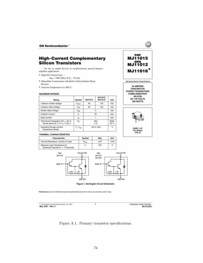
Figure A.1. Primary transistor specifications.
74
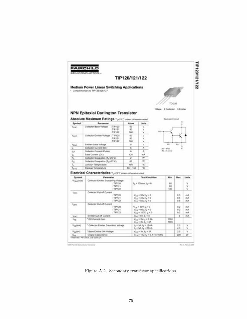
Figure A.2. Secondary transistor specifications.
75
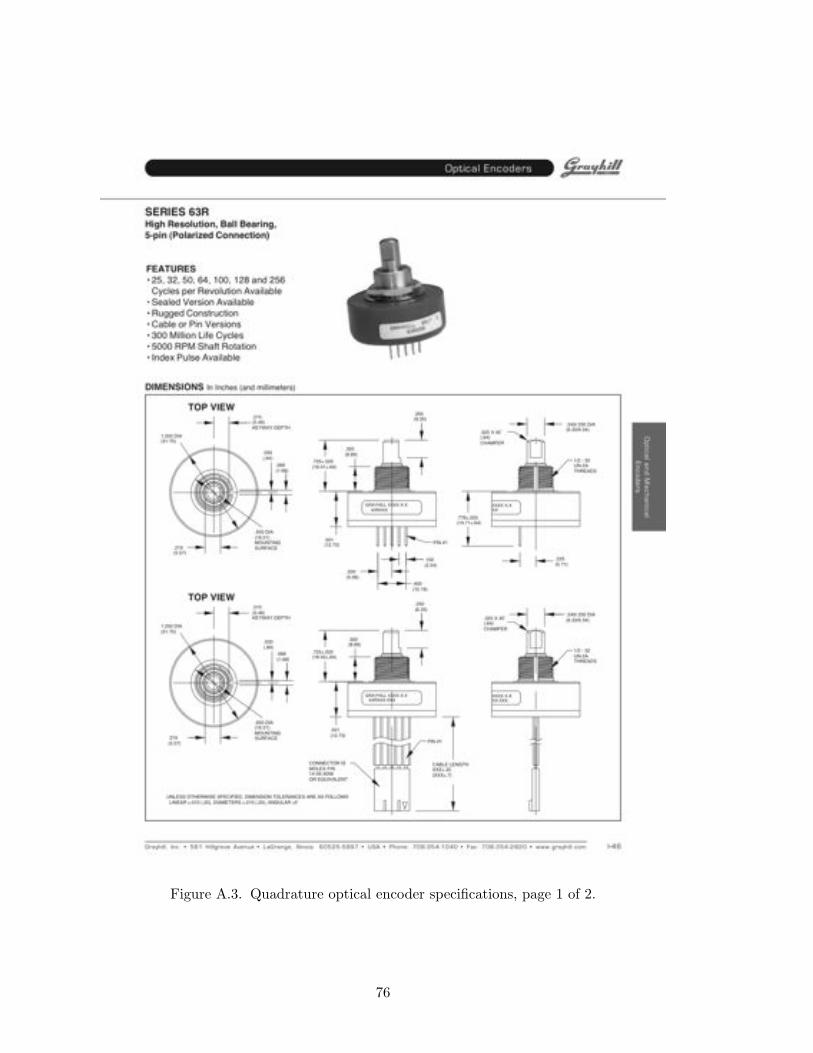
Figure A.3. Quadrature optical encoder specifications, page 1 of 2.
76
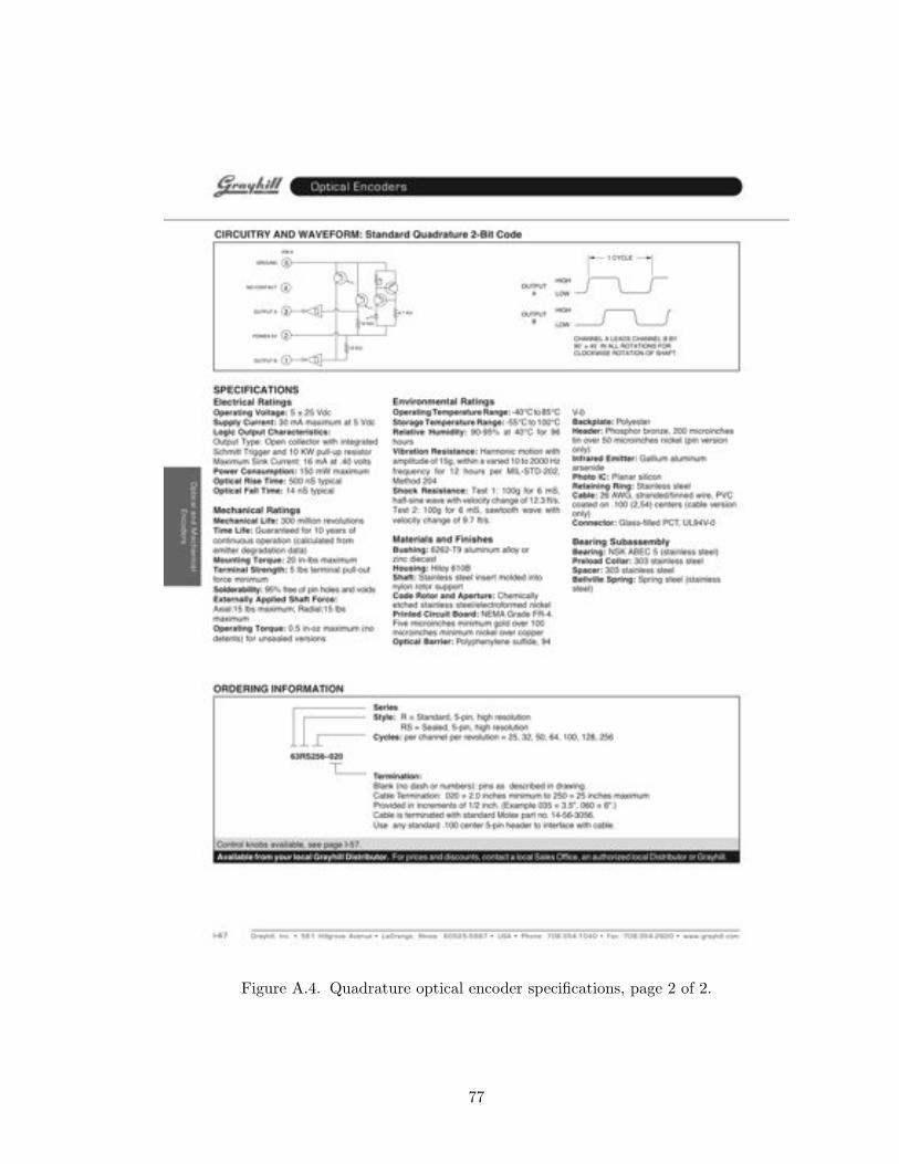
Figure A.4. Quadrature optical encoder specifications, page 2 of 2.
77

Figure A.5. Digital signal processor specifications, page 1 of 2.
78
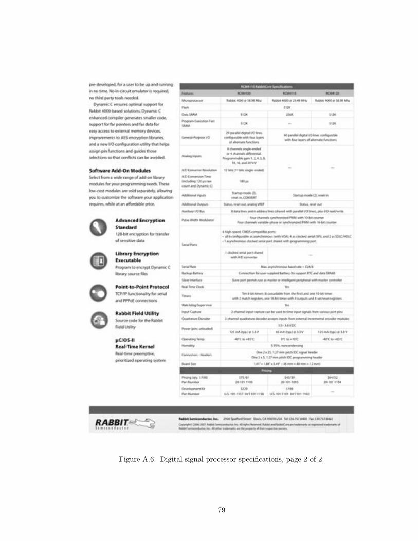
Figure A.6. Digital signal processor specifications, page 2 of 2.
79
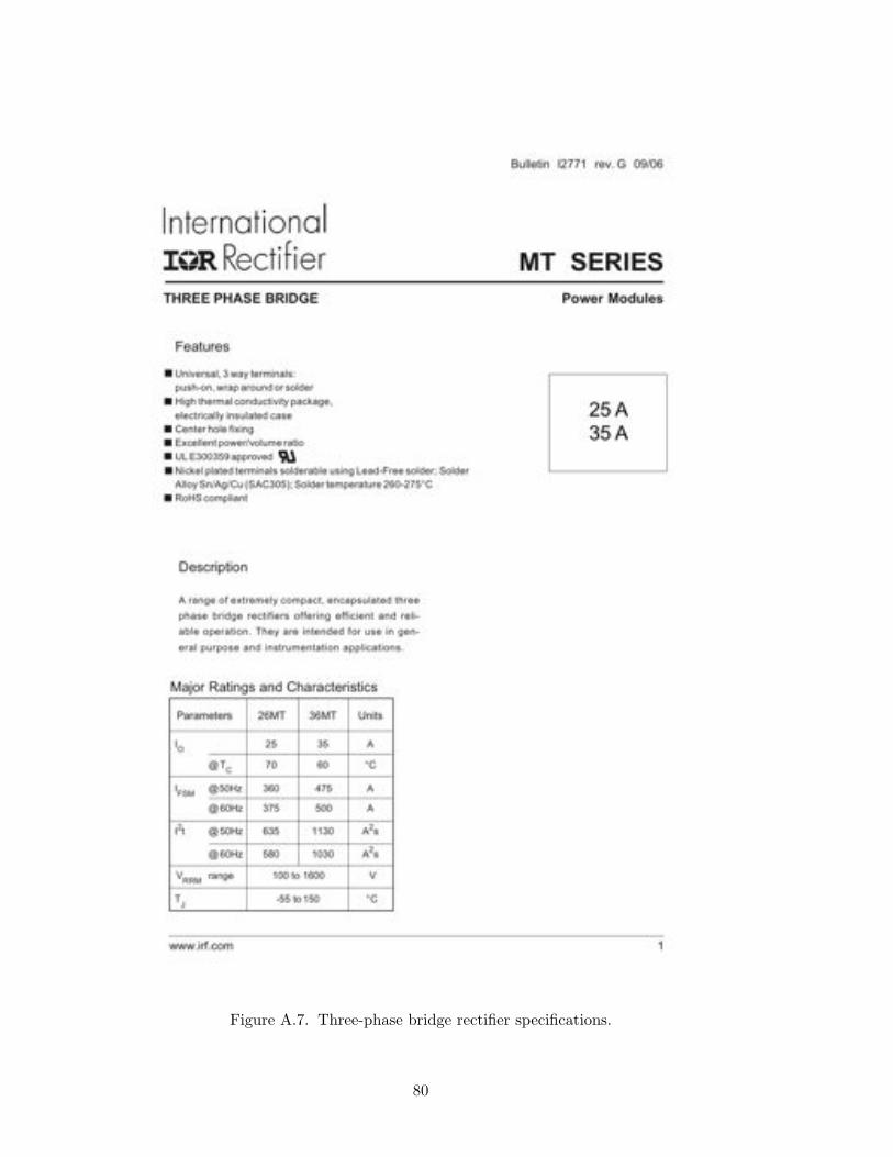
Figure A.7. Three-phase bridge rectifier specifications.
80

Figure A.8. Shunt resistor specifications.
81
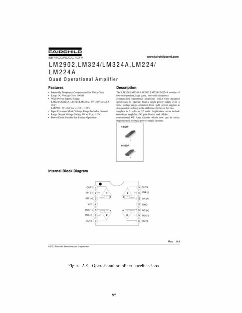
Figure A.9. Operational amplifier specifications.
82

Appendix B
Complete Control Program:Dynamic C Code
83
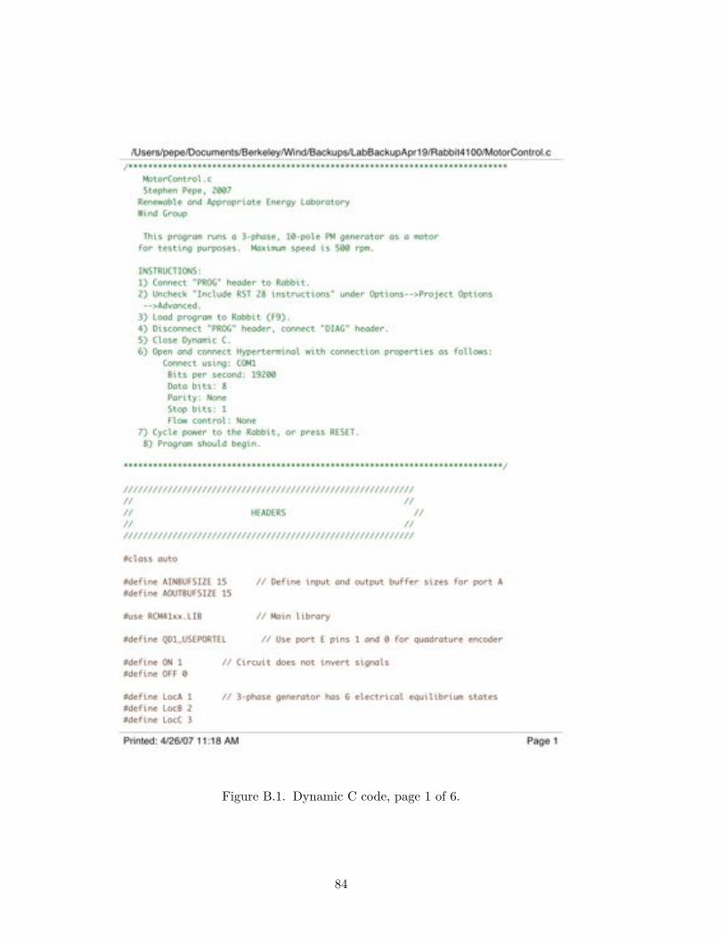
Figure B.1. Dynamic C code, page 1 of 6.
84
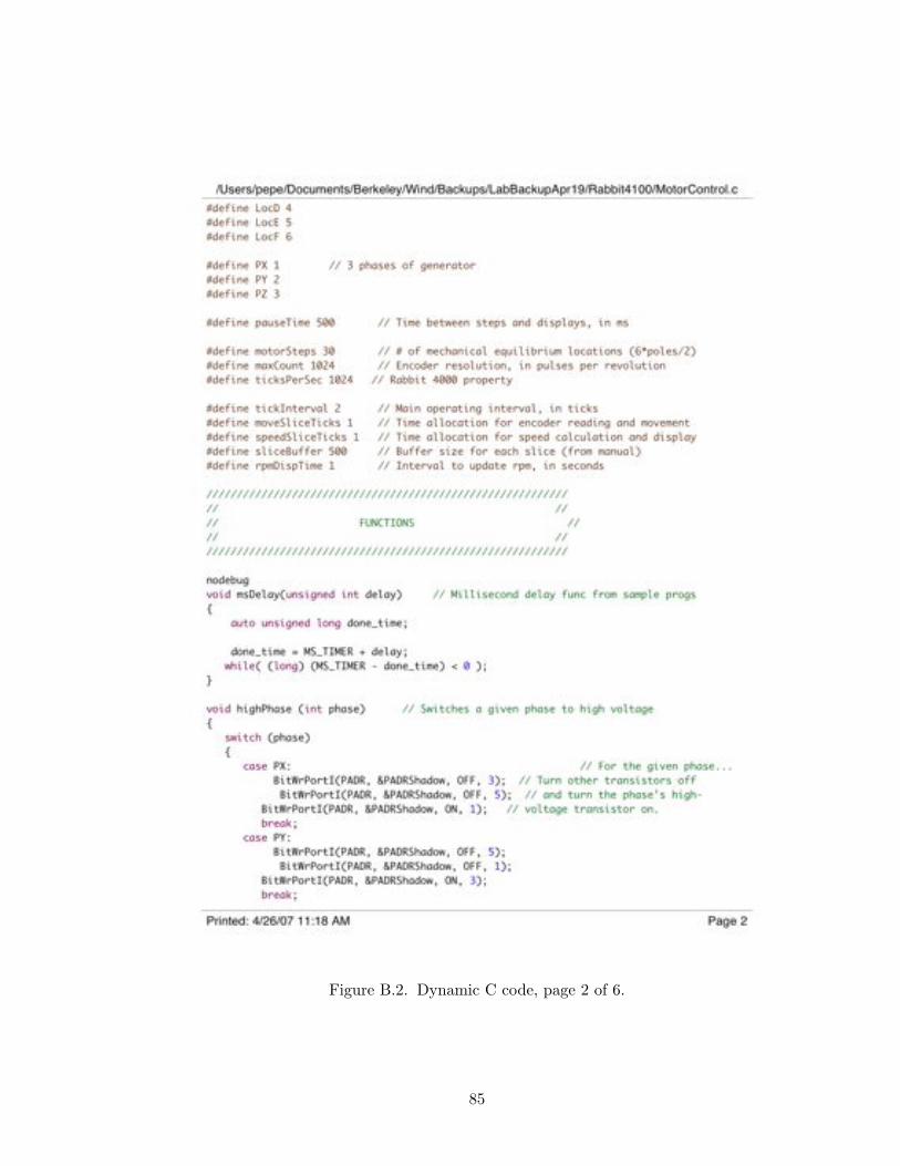
Figure B.2. Dynamic C code, page 2 of 6.
85
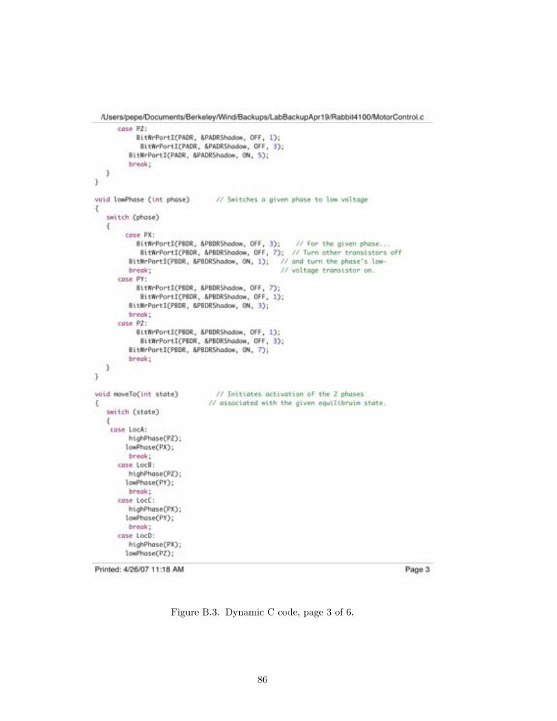
Figure B.3. Dynamic C code, page 3 of 6.
86
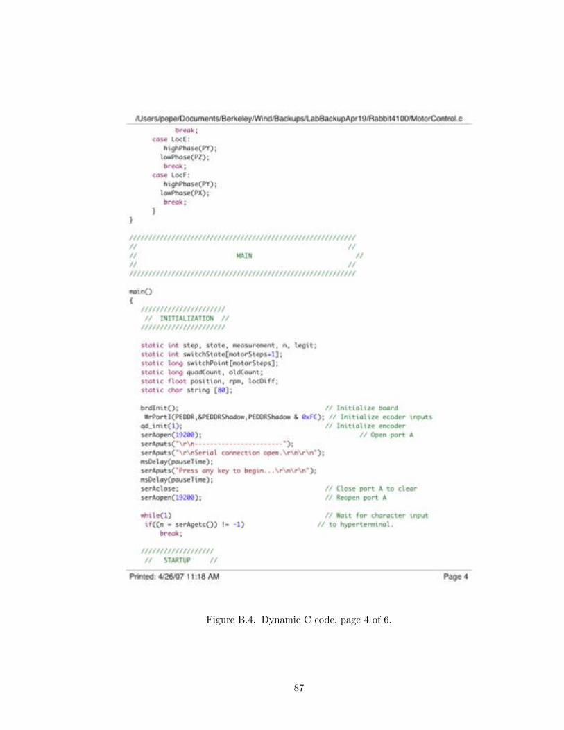
Figure B.4. Dynamic C code, page 4 of 6.
87
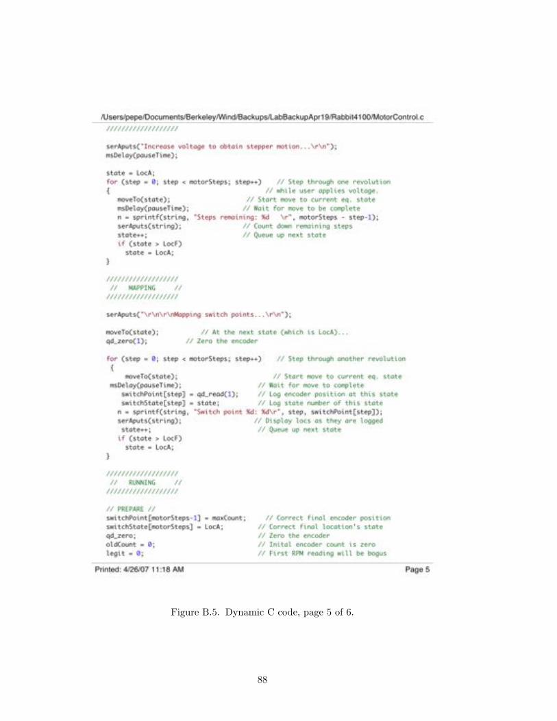
Figure B.5. Dynamic C code, page 5 of 6.
88
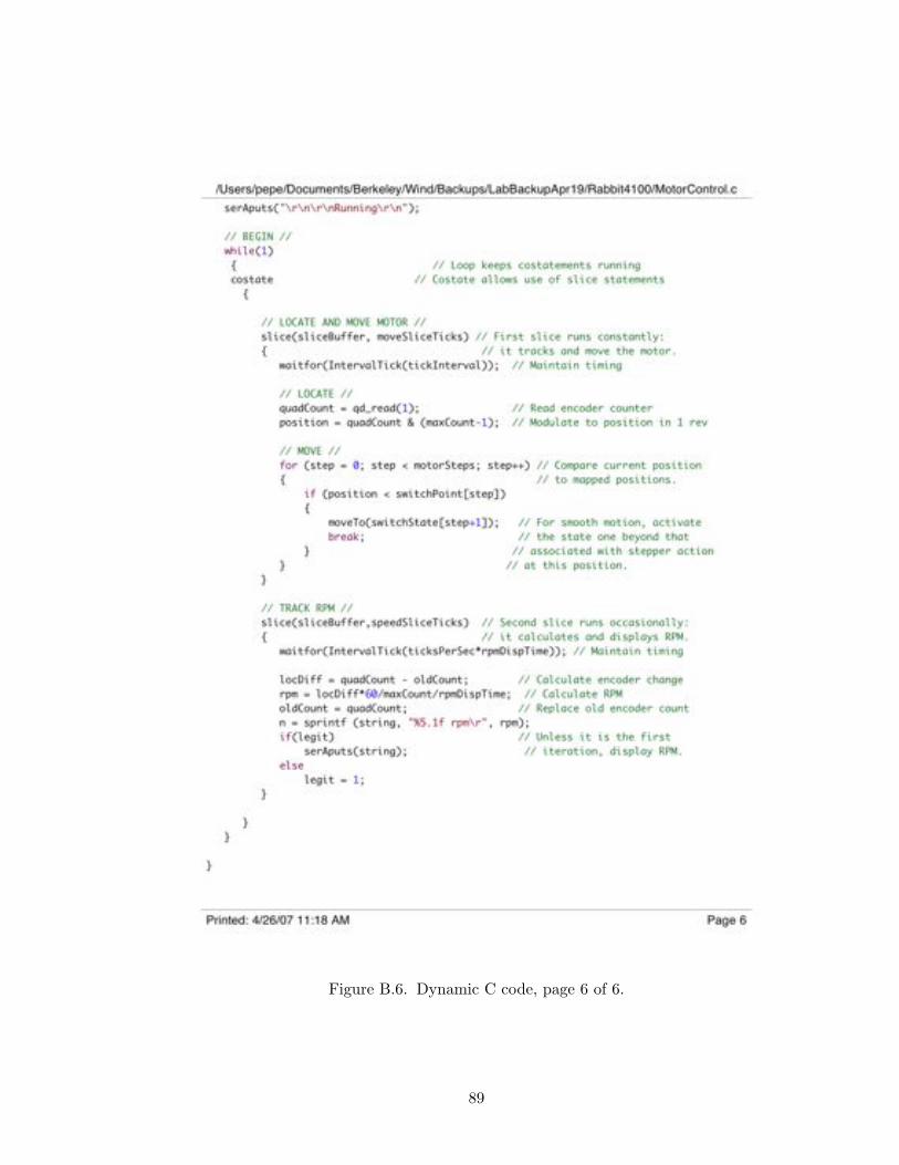
Figure B.6. Dynamic C code, page 6 of 6.
89

90
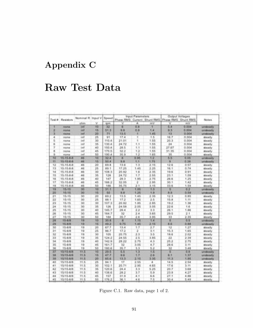
Appendix C
Raw Test Data
Figure C.1. Raw data, page 1 of 2.
91
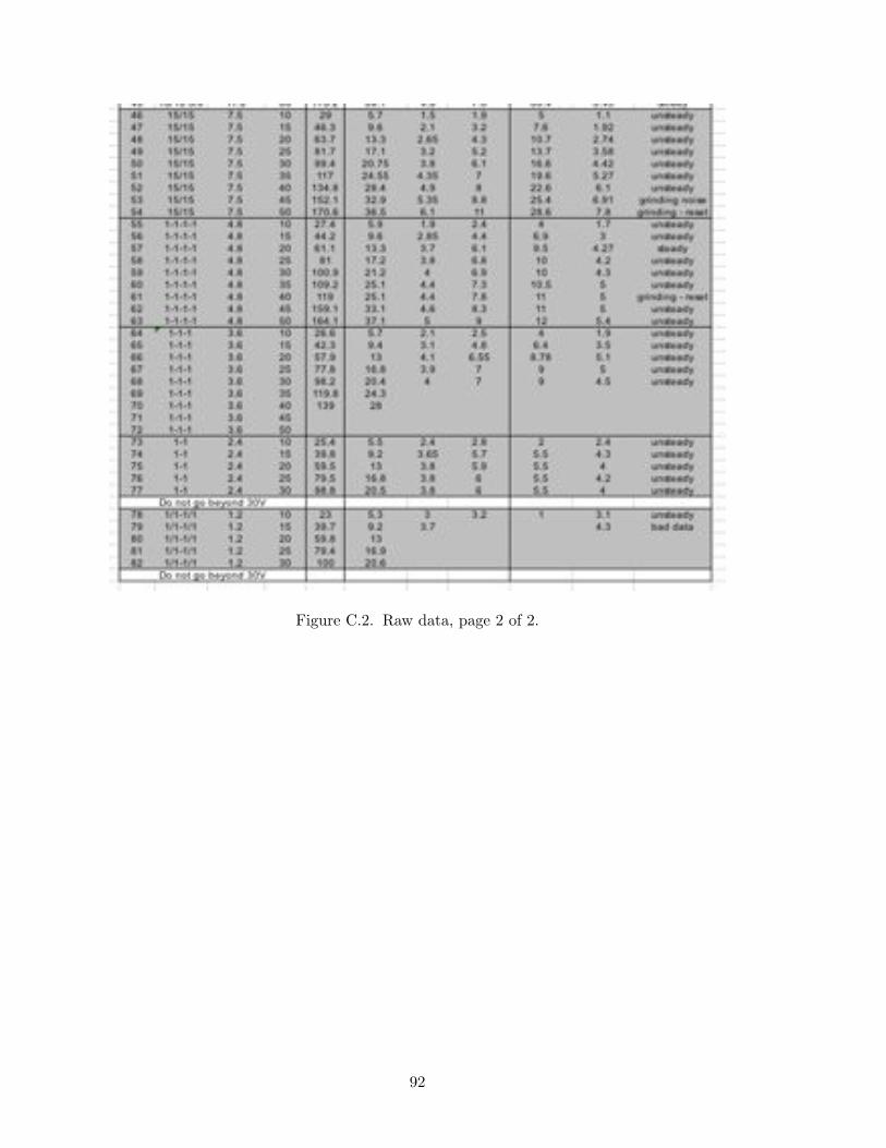
Figure C.2. Raw data, page 2 of 2.
92