Embed Size (px)
Citation preview
I
t, t -
.t
. - - - - - ~
AEDC-TR-77-80 ARCHIVE COPY- DO NOT LOAN
. f
AN ANALYSIS OF THE INFLUENCE OF SOME
EXTERNAL DISTURBANCES ON THE AERODYNAMIC
STABILITY OF TURBINE ENGINE AXIAL FLOW
FANS AND COMPRESSORS
P - - m
m = D m o - ==:m~
m B ~___ "n
" - " Z
E ~ =
E ~
ENGINE TEST F/~CILITY ARNOLD ENGINEERING DEVELOPMENT CENTER
AIR FORCE SYSTEMS COMMAND ARNOLD AIR FORCE STATION, TENNESSEE 37389
August 1977
Final Report for Period June 1973 -- June 1977
Approved for public release; distribution unlimited,
,'.', :" J; C I ' C e
Prepared for
DIRECTORATE OF TEST ENGINEERING DEPUTY FOR OPERATIONS ARNOLD ENGINEERING DEVELOPMENT CENTER AIR FORCE SYSTEMS COMMAND ARNOLD AIR FORCE STATION, TENNESSEE 37389
i . . . o . . . '
,- • .,.,: -:
NOTICES
When U. S. Government drawings specifications, or other data are used for any purpose other than a definitely related Government procurement operation, the Government thereby incurs no responsibility nor any obligation whatsoever, and the fact that the Government may have formulated, furnished, or in any way supplied the said drawings, specifications, or other data, is not to be regarded by implication or otherwise, or in any manner licensing the holder or any other person or corporation, or conveying any rights or permission to manufacture, use, or sell any patented invention that may in any way be related thereto.
Qualified users -may obtain copies of this report from the Defense Documentation Center.
References to named commercia! products in this report are not to be considered in any sense as an endorsement of the product by the United States Air Force or the Government.
This report has been reviewed by the Information Office (OI) and is releasable to the National Technical Information Service (NTIS). At NTIS. it will be available to the general public, including foreign nations.
APPROVAL STATEMENT
Tl~s technical report has been reviewed and is approved for publication.
FOR THE COMMANDER
MARION L. LASTER Director of Test Engineering Deputy for Operations
AEAN L. 7~E~VEREAU~"
Colonel, USAF Deputy for Operations
• -=' . ; : . . . . . . . :'~'.,~r..': . . . . . ~,."
UNCLASSIFIED REPORT DOCUMENTATION PAGE
t R E P O R T NUMBER J~ GOVT ACCESSION NO,
I AEDC-TR-77-80
4 TqTLE ( ~ d Subrrlte)
AN ANALYSIS OF THE INFLUENCE OF SOME EXTERNAL DISTURBANCES ON THE AERODYNAMIC STABILITY OF TURBINE ENGINE AXIAL FLOW FANS AND COMPRESSORS ? A u T H O R f s J
William F. Klmzey, ARO, I n c .
9 P E R F O R M I N G ORGAN~ZAT |ON NAME AND ADDRESS
A r n o l d E n g i n e e r i n g D e v e l o p m e n t C e n t e r A i r F o r c e S y s t e m s Command A r n o l d A i r F o r c e S t a t i o n , T e n n e s s e e 37389 I L C O N T R O L L I N G O F F I C E NAME AND ADDRESS
A r n o l d E n g i n e e r i n g D e v e l o p m e n t C e n t e r (XRFIS) A r n o l d A i r F o r c e S t a t i o n , T e n n e s s e e 37389 14 M O N ' T O R t N G AGENCY NAME & ADDRESSr | I d l l l e ren r / tom C o n t r o l l | n 8 0 ( h c e )
READ iNSTRUCTIONS BEFORE COMPLETING FORM
5 R E C I P I E N Y ' S C A T A L O G NUMBER
S T Y P E 0 F R E P O R T & P E R I O D C O V E R E D
F i n a l R e p o r t - J u n e 1973 - J u n e 1977
6 P E R F O R M I N G ORG R E P O R T NUMBER
B C O N T R A C T OR G R A N T NUMBER(e )
10 PROGRAM E L E M E N T P R O J E C T , TASK AREA & WORK UNIT NUMBERS
P r o g r a m E l e m e n t 6 5 8 0 7 F
1 :) R E P O R T D A T E
A u g u s t 1977 13 NUMBER O F PAGES
271 IS S E C U R I T Y CLASS. (e l IhJe report)
UNCLASSIFIED
ISe DECL ASSI F I C A T I O N DOWNGRADING SCNEOuLE N/A
16 D I S T R I B U T I O N S T A T E M E N T (o f th le Repor t )
A p p r o v e d f o r p u b l i c r e l e a s e ; d i s t r i b u t i o n u n l i m i t e d .
17 D I S T R I B U T I O N S T A T E M E N T (o f fhe n b l t r a c t enlered In B lock 30, I I d i f fe ren t .
l i t S U P P L E M E N T A R Y N O T F..~
A v a i l a b l e Ln DDC
19 K E Y WORO$ tCon tmue on reve r i e side f l n e c e s s e ~ ~ d i d e n t l l y by bloch number)
m a t h e m a t i c a l a n a l y s i s e n g i n e s c o m p r e s s o r s e x t e r n a l t u r b i n e d i s t u r b a n c e s a x i a l f l o w a e r o d y n a m i c s t a b i l i t y f a n s
2G J B S " R A C T (Cont inue ~ r e v e r i e side I ! necessary ~ d Jden|mfy ~ bJock numbe~
The o v e r a l l o b j e c t i v e o f t h e work d e s c r i b e d h e r e i n was t o d e v e l o p an i m p r o v e d m e t h o d f o r t h e c o m p u t a t i o n o f t h e i n f l u e n c e o f e x t e r n a l d i s t u r b a n c e s on t u r b i n e e n g i n e c o m p r e s s o r s t a b i l i t y , a n d , i n s o d o i n g , t o g a i n a d d e d p h y s i c a l i n s i g h t i n t o t h e d e s t a b i l i z i n g p r o c e s s e s . The o b j e c t i v e s w e r e a c c o m p l i s h e d t h r o u g h t h e d e v e l o p m e n t o f a o n e - d i m e n s i o n a l , t i m e - d e p e n d e n t m a t h e m a t i c a l c o m p r e s s o r m o d e l f o r a n a l y s i s o f p l a n a r d i s t u r b a n c e s and an
FORM 1473 E D I T I O N O F I N O V 6 S I S O B S O L E T E DD , JAN 73
UNCLASSIFIED
UNCLASSIFIED
20. ABSTRACT ( C o n t i n u e d )
e x t e n s i o n o f t h e model t o a t h r e e - d i m e n s i o n a l fo rm f o r a n a l y s i s o f d i s t o r t e d i n f l o w s . The m o d e l s s a t i s f y m a s s , momentum and e n e r g y e q u a t i o n s on a t i m e - d e p e n d e n t b a s i s . C o m p r e s s o r s t a g e f o r c e and s h a f t work w e r e d e t e r m i n e d f rom e m p i r i c a l s t a g e c h a r a c t e r i s t i c s w i t h c o r r e c t i o n s made f o r u n s t e a d y c a s c a d e a i r f o i l a e r o d y n a m i c s . The s y s t e m o f e q u a t i o n s c o m p r i s i n g t h e mode l i s s o l v e d u s i n g a d i g i t a l c o m p u t e r . Example p r o b l e m s w i t h c o m p a r i s o n s t o e x p e r i m e n t s a r e p r e s e n t e d f o r t h r e e d i f f e r e n t c o m p r e s s o r s . Example p r o b l e m s s o l v e d u s i n g t h e o n e - d i m e n s i o n a l a n a l y s i s i n c l u d e : d e t e r m i n a t i o n o f t h e s t e a d y - s t a t e s t a b i l i t y l i m i t ( s u r g e l i n e ) w i t h u n d i s t u r b e d f l o w , i n s t a b i l i t y c a u s e d by o s c i l l a t i n g p l a n a r i n f l o w , dynamic r e s p o n s e o f a c o m p r e s s o r t o o s c i l l a t i n g e n t r y p r e s s u r e , dynamic r e s p o n s e t o o s c i l l a t i n g d i s c h a r g e p r e s s u r e , and c o m p r e s s o r i n s t a b i l i t y c a u s e d by r a p i d upward ramps o f e n t r y t e m p e r a t u r e . Example p r o b l e m s s o l v e d u s i n g t h e d i s t o r t i o n model i n c l u d e : s t a b i l i t y l i m i t ( s u r g e ) l i n e r e d u c t i o n c a u s e d by a combined r a d i a l and c i r c u m f e r e n t i a l p r e s s u r e d i s t o r t i o n , t i m e - v a r i a n t d i s t o r t i o n e f f e c t s , p u r e r a d i a l p r e s s u r e d i s t o r t i o n e f f e c t s , and p u r e p r e s s u r e and t e m p e r a t u r e c i r c u m f e r e n t i a l d i s t o r t i o n e f f e c t s . C o m p a r i s o n s a r e made w i t h e x p e r i m e n t a l r e s u l t s , and t h e m o d e l s d e v e l o p e d a r e shown t o c o m p u t e t h e c o m p r e s s o r s t a b i l i t y l i m i t s w i t h r e a s o n a b l e a c c u r a c y .
A F S r A , ~ l r AFIL T e n q
UNCLASSIFIED
A E D C-T R -77-80
PREFACE
The research reported herein was partially performed
by the Arnold Engineering Development Center (AEDC), Air
Force Systems Co,and (AFSC). The work and analysis for
this research were done by personnel of ARO, Inc., AEDC
Division (a Sverdrup Corporation Company), operating
contractor for the AEDC, AFSC, Arnold Air Force Station,
Tennessee, under Program Element 65807F. A portion of the
work was conducted under ARO Projects No. RF435-12YA,
R32P-98A, R32P-12YA, R32P-50A, and R32P-C5A. The author
of the report is William F. Kimzey, ARO, Inc. Eules L.
Hively is the Air Force project manager. The manuscript
(ARO Control No. ARO-ETF-TR-77-47) was submitted for
publication on July 12, 1977.
The author wishes to acknowledge Mr. Fran Loper, ARO,
Inc., for his assistance in the development of numerical
analysis and computer programs required for this effort;
Mr. Don Couch and Mr. Ted Garretson, ARO, Inc., for their
work in computer program development and in running some
of the data presented in this report; and Dr. B. H. Goethert,
University of Tennessee Space Institute, for assistance
provided during the course of this work. The material re-
ported herein was submitted to the University of Tennessee as
partial fulfillment of the requirements of the degree of
Doctor of Philosophy.
A EDC-TR-7?-80
CONTENTS
Chapter Pag___~e
I. INTRODUCTION . . . . . . . . . . . . . . . . . . 1
Ramifications of Stability to Engine
Operation . . . . . . . . . . . . . . . . . . 3
Major Operating Conditions and External
Disturbances Influencing Stability ..... 3
Previous Analyses of Compressor Stability
with Undisturbed Flow . . . . . . . . . . . . 8
Previous Analyses of Compressor Stability
with Disturbed Flow . . . . . . . . . . . . . 12
Objectives and Approach of Current Work .... 19
Organization . . . . . . . . . . . . . . . . . 22
II. DEVELOPMENT OF ONE-DIMENSIONAL,
TIME-DEPENDENT MODEL . . . . . . . . . . . . . 23
Governing Equations . . . . . . . . . . . . . . 24
Stage Forces and Shaft Work . . . . . . . . . . 29
Method of Solution . . . . . . . . . . . . . . 43
III. EXAMPLE PROBLEMS WITH COMPARISON TO
EXPERIMENTS, ONE-DIMENSIONAL MODEL ...... 60
Steady-State Stability Limits . . . . . . . . . 61
Dynamic Stability Limits . . . . . . . . . . . 66
IV. DEVELOPMENT OF THREE-DIMENSIONAL MODEL
FOR DISTORTED FLOWS . . . . . . . . . . . . . . 78
Governing Equations . . . . . . . . . . . . . . 79
iii
AEDC-TR-77-80
Chapter
Simplifications . . . . . . . . . . . . . . . .
Special Considerations for Distortion
Effects . . . . . . . . . . . . . . . . . . .
Method of Solution . . . . . . . . . . . . . .
V. EXAMPLE PROBLEMS WITH COMPARISON TO
EXPERIMENTS, DISTORTION MODEL . . . . . . . . .
Combined Distortion Pattern,
XC-1 Compressor . . . . . . . . . . . . . . .
Time-Variant Distortion . . . . . . . . . . . .
Pure Radial and Circumferential
Distortion Patterns . . . . . . . . . . . . .
VIo SUMMARY OF RESULTS AND RECOMMENDATIONS
FOR FURTHER WORK . . . . . . . . . . . . . . .
One-Dimensional, Time-Dependent Analysis . . .
Distortion Analysis . . . . . . . . . . . . . .
Recommendations for Further Work . . . . . . .
BIBLIOGRAPHY . . . . . . . . . . . . . . . . . . . . .
Page
86
92
i01
109
109
115
117
122
123
126
129
133
A E DC-TR-77-80
ILLUSTRATIONS
Figure Page
1. Typical Aircraft Gas Turbine Compression
System Configurations . . . . . . . . . . . . . 142
2. Typical Compressor Map . . . . . . . . . . . . . 143
3. Effect of Flight Altitude and Mach Number on
Compressor Operating Region . . . . . . . . . . 144
4. Typical Influences of External Disturbances
on Compressor Stability . . . . . . . . . . . . 146
5. Surge Analysis Based on Compressor and
Throttle Curve Shapes . . . . . . . . . . . . . 149
6. Representative Axial Flow Compressor
Arrangement and Operation . . . . . . . . . . . 150
7. Physical System Modeled and Control Volumes. . . 151
8. Rotor Fluid Element Velocities and Forces. . . 152
9. Representative Stage Characteristics [46] .... 153
I0. Steady-State and Unsteady Stage
Characteristic Behavior . . . . . . . . . . . . 154
ii. Unsteady Airfoil and Cascade Aerodynamics .... 155
12. Comparison of Theoretical and Experimental
Unsteady Cascade Lift Coefficients ...... 156
13. Variation of Dynamic Lift Coefficient Ratio
with Mean Angle of Attack . . . . . . . . . . . 157
14. Unsteady Lift Coefficient Magnitude Ratio .... 158
Y
AEDC-TR-77-80
ri~e
15. Computational Plane Designations for Finite
Difference Solutions . . . . . . . . . . . . . 159
16. Solution Procedure for One-Dimensional,
Time-Dependent Model . . . . . . . . . . . . . 160
17. Station Locations (Computation Planes) for
One-Dimensional, Time-Dependent Models .... 161
18. XC-I Compressor Model Loaded to Stall,
N//~ = 90% . . . . . . . . . . . . . . . . . . 162
19. Flow Breakdown Process Leading to Instability,
XC-I Compressor, N//~ = 90% .......... 163
20. Comparison of Model Computed 90% Speed
Characteristic and Stability Limit with
Experimenual Measurements, XC-I Compressor . . 164
21. NACA-8 Compressor Model Loaded to Stall,
N//~ = 90% . . . . . . . . . . . . . . . . . . 165
22. Comparison of Model Computed Speed Character-
istics and Stability Limits with Experimental
Measurements, NACA-8 Compressor ........ 168
23. Comparison of Model Computed Flow Coefficients
at Compressor Stability Limit with
Experimental Measurements,
NACA-8 Compressor . . . . . . . . . . . . . . . 169
24. Comparison of Model Computed Speed Character-
istics and Stability Limits with Experimental
Measurements, J85-13 Compressor ........ 171
vi
AE DC-T R-77-80
Figure Page
25. Oscillating Inflow Loading to Stall,
NACA-8 Compressor, N//~ = 70% . . . . . . . . . 172
26. Stability Limits for Planar Oscillating
Inflow, NACA-8 Compressor . . . . . . . . . . . 179
27. Test Arrangements for NASA J85-13 Dynamic
Response Experiments . . . . . . . . . . . . . 180
28. Variation of Amplitude Ratio and Phase Angle
Through the J85-13 Compressor with
Oscillating Compressor Entry Pressure
at 40 Hz . . . . . . . . . . . . . . . . . . . 181
29. Dynamic Response to Oscillating Compressor
Entry Pressure, J85-13 Compressor ....... 183
30. Variation of Amplitude Ratio and Phase Angle
Through the J85-13 Compressor with
Oscillating Engine Fuel Flow at 40 Hz . . . . 189
31. Dynamic Response to Oscillating Fuel Flow,
J85-13 Compressor . . . . . . . . . . . . . . . 191
32. Rapid Inlet Temperature Ramp to Stall,
NACA-8 Compressor . . . . . . . . . . . . . . . 193
33. Compressor Instability Caused by Rapid Inlet
Temperature Ramps . . . . . . . . . . . . . . . 196
34. Division of Compressor into Control Volumes. . . 197
35. Control Volume Velocities and Fluxes ...... 198
36. Circumferential Crossflow . . . . . . . . . . . . 199
37. Radial Crossflow . . . . . . . . . . . . . . . . 200
vii

AE DC-TR-77-80
Figure Page
38. Radial Distortion Effects . . . . . . . . . . . . 201
39. Circumferential Distortion Effects ....... 202
40. Compressor Entry Total Pressure Distribution
for Combined Distortion Pattern ........ 205
41. Compressor Entry Pressure Input Values for
Combined Distortion Pattern . . . . . . . . . . 206
42. Comparison of Computed and Experimental
Stability Limits with Combined Distortion
Pattern, XC-I Compressor . . . . . . . . . . . 207
43. Circumferential Profiles in Tip Region with
Combined Distortion Pattern,
XC-I Compressor 208 I m a l o o D e e m e e i i o m
44. Comparison of Computed and Measured
Circumferential Distortion Attenuation for
Combined Pattern . . . . . . . . . . . . . . . 210
45. Radial Profiles with Combined Distortion
Pattern . . . . . . . . . . . . . . . . . . . . 213
46. Radial Profiles with Uniform Entry Flow ..... 215
47. Flow Coefficient Distribution Just Prior to
Instability with Combined Distortion
Pattern . . . . . . . . . . . . . . . . . . . . 217
48. Time-Variant Distortion . . . . . . . . . . . . . 221
49. Relative Frequency Spectrum for Time-Variant
Distortion Pattern . . . . . . . . . . . . . . 222
50. Loss in Stability Limit Pressure Ratio with
Time-Variant Distortion . . . . . . . . . . . . 223
°,°
ym
AEDC-TR-77-80
Figure Page
51. Computed Radial Distortion Influences on
Stability . . . . . . . . . . . . . . . . . . . 224
52. Comparison of Radial Distortion Model
Computations with Experimental Results .... 226
53. Model Computed Influence of Circumferential
Pressure Distortion on Stability,
XC-I Compressor . . . . . . . . . . . . . . . 227
54. Comparison of Circumferential Distortion
Model Computations with Experimental
Results . . . . . . . . . . . . . . . . . . . . 228
55. Circumferential Crossflow Magnitudes and
Effects . . . . . . . . . . . . . . . . . . . . 229
56. Model Computed Influence of Circumferential
Distortion Angular Extent on Stability,
XC-I Compressor . . . . . . . . . . . . . . . . 231
57. Effect of Unsteady Airfoil Stall Properties
on Stability Margin . . . . . . . . . . . . . . 232
58. Model Computed influence of Circumferential
Temperature Distortion on Stability,
XC-I Compressor . . . . . . . . . . . . . . . . 233
59. Comparison of Circumferential Temperature
Distortion Model Computations with
Experimental Results . . . . . . . . . . . . . 234
AED C-TR-77-80
APPENDIXES
A. FIGURES FOR CHAPTERS I THROUGH VI . . . . . . . .
B. COMPRESSOR DETAILS AND STAGE
CHARACTERISTICS . . . . . . . . . . . . . . . .
C. FIGURES AND TABLES FOR APPENDIX B . . . . . . . .
NOMENCLATURE . . . . . . . . . . . . . . . . . . . . .
141
235
237
265
X
A E DC-T R-77-80
CHAPTER I
INTRODUCTION
Stable aerodynamic operation of the compression
system of an aircraft gas turbine engine is essential for
the engine to operate safely and to satisfactorily deliver
the performance which it is designed to provide. The com-
pression system of an aircraft gas turbine engine consists
of one or more compressors arranged in configurations such
as those illustrated in Fig. 1 (Appendix A). 1 Aerody-
namically stable operation refers to the condition in which
the compressor delivers a desired quantity of airflow on a
continuous basis, compressed to a desired pressure level,
free of excessively large amplitude fluctuations in the flow
properties throughout the compressor. The aerodynamic
stability limit is most commonly represented as a locus of
corrected rotor speed points denoting the minimum corrected
flow rate value for stable operation on a plot of the total
pressure ratio across the compressor versus corrected air-
flow rate as shown in Fig. 2. Operation to the right of the
curve is stable and to the left of the curve is unstable.
The stability limit curve is often referred to as
the surge line or stall line of the compressor stemming from
IAII figures in Chapters I through VI appear in Appendix A.
A E DC-T R-77-80
the fact that surge is one possible specific form of
instability experienced in compressors, and all compressor
instabilities are initiated by aerodynamic stall of some
blades or vanes of the compressor.
The stability margin of the compressor is commonly
taken to be the percentage difference between the compressor
total pressure ratio at the stability limit and that at the
operating line holding corrected airflow constant (Fig. 2).
The position of the operating line is primarily determined
by the load imposed on the compressor by downstream engine
components. However, under actual flight conditions in an
aircraft, the positions of both the stability limit line and
the operating line are influenced by external disturbances
in the flow at either the entry or exit of the compressor.
The overall objective of this study is to develop
an improved analytical method which will allow prediction of
the loss of stability margin of the compressor caused by
external disturbances imposed upon it by flight conditions
in an aircraft. Also, the development of the method is
intended to provide some degree of physical understanding of
the processes which lead to compressor instability.
Prior to beginning the analysis it is helpful to
review the ramifications of stability on engine operation
and to review some of the experimentally observed influences
of the operating conditions and external disturbances on
compressor stability. Also, a review of some of the
AEDC-TR -77-80
previously accomplished works directed at stability pre-
dictions both with and without external disturbances will be
made.
I. RAMIFICATIONS OF STABILITY TO ENGINE OPERATION
Operation of the compressor to the left of the
stability limit (Fig. 2) will result in loss of thrust,
possible loss of engine control, or possible engine
structural damage caused by overheating and high cyclic
stress induced in the engine by unstable flow conditions.
Reference [1] 2 presents evidence of thermal and cyclic
stress effects imposed by compressor instability for one
particular engine. Montgomery [2] has compiled a history of
difficulties in the operation of several aircraft gas
turbine engines which have been experienced because of
compressor stability problems. Montgomery's work well
illustrates the need for a method of determining the sta-
bility limit of the gas turbine engine compressor,
especially as they are affected by the conditions of flight.
II. MAJOR OPERATING CONDITIONS AND EXTERNAL
DISTURBANCES INFLUENCING STABILITY
The position of the stability limit line and the
operating line of the compressor of a given design are
2Numbers in brackets refer to similarly numbere~ references in the Bibliography.
AE DC-T R-77-80
affected in flight by the condition of the flow entering the
compressor and by the throttling or back pressure provided
by the compressor or engine component downstream of the
compressor under consideration. The entry total tempera-
ture, the Reynolds number at which the compressor must
operate, and the nonuniformity and unsteadiness of the flow
at the compressor inlet have major influences on the sta-
bility of the compressor.
Because of the variation of total temperature at
the compressor entry which occurs with flight Mach number
and altitude, the compressor's operating region moves far
from the design point of the compressor; thus, a relatively
large region of the compressor map must be considered in any
analysis of stability. Figure 3a depicts the variation of
operating region with compressor inlet total temperature for
a simple single spool turbojet compressor. Figure 3b shows
the influence of flight Mach number and altitude on engine
entry total temperature. The changes in flight conditions
cause the Reynolds number to change. Figure 3c gives an
example of the Reynolds number influence on the stability
limit. The Reynolds Number Index (REI) used in Figure 3c is
the ratio of the Reynolds number in flight to that which
would exist at sea-level-static conditions at the same
compressor inlet axial Mach number. Figure 3d shows the
variation of REI with flight condition.
Figure 4 shows experimentally determined losses in
stability margin caused by nonuniform (distorted) flow
4
AE DC-TR-77-80
conditions and unsteady flow conditions at the compressor
entry plane. In Fig. 4 the loss is illustrated by downward
shifts of the stability limit toward the operating line. In
some cases, the disturbances also cause stability margin
loss by moving the operating line upward. For purposes of
illustration, the entire loss is shown in Fig. 4 as a down-
ward movement of the stability limit. Figure 4a from [4] is
for the case of steady but distorted flow into the com-
pressor created by a wire screen of nonuniform porosity
placed in front of the compressor. Figure 4b from [5]
illustrates the loss in stability margin caused by uniform
but sinusoidally time-varying flow into the compressor
produced by a rotating flow interrupter upstream of the
compressor. The case of combined unsteady and distorted
flow, sometimes called time-variant distortion, is shown in
Figs. 4c and 4d for a turbojet engine compressor [6] and a
turbofan engine fan [7]. The engine entry flow fields were
produced by a venturi-centerbody arrangement which produced
an unstable shock wave boundary layer interaction which
causes the adverse flow field at the engine entry plane [6].
Figure 43, based on data from [8], indicates the influence
on the downstream compressor stability limit line of the
nonuniform and unsteady flow field exiting from a forward
compressor of a turbofan engine.
In addition to disturbances in the pressure enter-
ing the compressor, total temperature disturbances may occur.
Information from [9] shown in Fig. 4f, indicates the
A EDC-TR-77-80
experimentally determined influence of time-steady spatial
variation o[ total temperature entering the compressor.
Rapid uniform total temperature increases at the engine
inlet which could be caused by ingestion of hot gases pro-
duced by gun or rocket fire can also cause a loss of
stability [10].
Disturbances to the compressor may originate at
the exit of the compressor as well as at the inlet. An
experiment conducted on a turbofan engine described in [ii]
demonstrated the influence of an oscillating back pressure
on fan stability.
The distortion examples of Fig. 4 all use total
pressure or total temperature variation to describe the
distortion pattern characteristics and to correlate with
loss in stability margin. The use of total pressure and
total temperature has been shown through experience and is
accepted in practice to be the most practical distortion
pattern description method (see Bibliography). The
Society of Automotive Engineers Aerospace Recommended
Practice on Gas Turbine Engine Inlet Flow Distortion
Methodology [12] specifies total pressure as the parameter
for distortion pattern description. Total pressure and
total temperature are used because they are much more
readily measured than velocity distribution, static pressure
and flow direction. Also, when a distorted flow field
approaches an engine, the interaction of the engine with the
distortion pattern produces a specific static pressure,
6
AEOC-TR-77-80
velocity and flow angularity pattern at the engine entry
(di&cussed in Chapter IV). Thus, the combination of a total
pressure or total temperature distortion pattern with an
engine at a given operating condition implicitly specifies
a velocity, static pressure and flow direction distribution
at the compressor entry and throughout the compressor.
Measurement of velocity and flow direction at the compressor
entry is sometimes suggested as a more physically meaningful
set of measurements for distortion pattern definition
because rotor blade angle of attack is related to the
velocity vectors at the rotor blade leading edge. However,
compressor instability caused by distortion can (and often
does) occur because of stall in any stage of the compressor.
Therefore, unless detailed velocity and flow direction
measurements are made at each and every compressor stage
entry, no real additional information is provided by the
more difficult velocity and flow direction measurements.
Further, the total pressure and total temperature distri-
butions produced by an aircraft inlet, if measured approxi-
mately an engine diameter ahead of the compressor entry
plane, will be the same with or without an engine installed
behind the inlet. Therefore, distortion pattern information
from scale model and full-scale inlet tests may be obtaaned
without the engine installed. This could not be done if
velocity static pressure and flow direction were chosen as
the distortion pattern definition parameters. For these
reasons, total pressure and total temperature variations
AE DC-TR-77-80
will also be used for disturbance description for the
analytical work in this study.
Most of the influences shown in Fig. 4 were
determined from simulations of actual flight in altitude
test cells or wind tunnels using artificial methods of dis-
turbance generation. These disturbances are, however,
representative of actual disturbances experienced in flight.
The influence on stability in actual flight is, however,
more difficult to measure; thus, the ground test sources are
used. More detailed information on the generation of these
disturbances in flight is given in [13 through 16].
III. PREVIOUS ANALYSES OF COMPRESSOR STABILITY
WITH UNDISTURBED FLOW
Early analysis of compressor instability dealt
with "surging" described as "a violent fluctuation in
delivery" by Whittle in an early work (1931) on the turbo-
compressor as a supercharger [17]. In an even earlier work
by Kearton [18] and in later works by Den Hartog [19] and
IIorlock [20], analysis of surge was performed using the
shapes of the pressure-ratio-mass flow curves of the com-
pressor and the throttle (back pressuring device) to locate
stable and unstable combinations of the compressor and
throttle and to qualitatively describe surging. (Figure 5
is a simple illustration of this analysis.) With the
throttle set to an open condition, the match point, A, is a
stable operating condition. This may be deduced by
8

AE DC-T R-77-80
imagining that the flow is momentarily perturbed upward, if
this should happen, the upward perturbation will cause a
reduction in the pressure exiting from the fan, and an
increase in the resistance to flow from the throttle. Both
of these effects tend to cause flow to decrease, thus
countering the original perturbation and restoring equi-
librium. A similar argument applies for a downward
perturbation of flow rate. If, however, the match point is
point C, instability will occur. Once more, imagine an
upward perturbation of flow. This will result in an
increase in compressor discharge pressure which is greater
than the increase in resistance to flow; thus, the upward
perturbation in flow will be reinforced causing the flow to
continue to increase. Thus, point C is unstable. This
analysis may be generalized to state that the compressor-
throttle combination will be unstable in regions where the
slope of the compressor characteristic curve is greater than
the slope of the throttle loss characteristic curve.
Applying this rule, if operation is attempted near point C,
and the flow is perturbed upward, it will continue to
increase until it reaches point B where the flow increase is
countered (that is, the compressor characteristic slope
becomes less than the throttle curve slope) and, ignoring
dynamic effects, is caused to begin to decrease. Once the
flow starts down, however, it will continue to decrease
until it reaches a region near point D where the slope of
the compressor characteristic is once more less than that of
9
A EDC-TR-77-80
the loss characteristic. Thus, a limit cycle, quaiitatively
describing surge based on characteristic curve nonlinearity,
but ignoring dynamic effects, is constructed.
This simple explanation provided a reasonable
qualitative explanation of the surge instability, but in
actual use tended to predict a value of flow rate at which
surge would be encountered which was often lower than that
actually experienced [21]. It later became common practice
to assume that instability would occur at the peak com-
pressor ratio; that is, at the first point where the
compressor characteristic slope became positive. This
assumption was reasonably well borne out for high corrected
rotor speeds by experiments [21, 22].
While the theories described to this point were
based principally on observations made on centrifugal com-
pressors, they are in principle applicable to axial flow
units. (For example, the compressor characteristic curve of
Fig. 5 in no way specifies the type of compressor which
produced it.) Pearson and Bowmer (1949) [21] specifically
addressed the problem of stability in axial flow compressors.
Pearson and Bowmer observed the discrepancy which existed
between compressor experiments and the simple nonlinear
characteristic curve theory and noted that the nonlinear
theory ignored the dynamic effects caused by volumetric
capacitance, fluid column inertia, and flow resistance in
the compressor and ducting. Pearson and Bowmer approached
the problem by deriving an approximate set of dynamic
I0
AEDC-TR-77-80
(time-dependent) equations for a twelve-stage axial flow
compressor and related the compressor to an analogous
electrical circuit. The compressor was stacked from assumed
stage characteristics to form a representative multi-stage
unit. It was then assumed that instability would occur at
any condition where the impedance of any given part of the
circuit representing a stage was zero. For positive
impedance, disturbances in the circuit would be damped; for
negative impedance the disturbances would be amplified, thus
causing instability.
Howell (1964) [23] extended the work of Pearson
and Bowmer by applying the same technique of drawing an
electrical analogy to the compressor, but used a more
detailed stability analysis on the resulting electrical net-
work. Howell also applied the analysis to an actual
compressor and compared those results to the experimentally
determined stability limit. Howell's analysis produced a
reasonably good prediction of the stability limit, but it
was somewhat below the experimentally observed limit at
design rotor speed.
Kimzey and Couch (1969) developed a stability
criterion for predicting the position of the stability limit
directly from an analysis of a simple set of dynamic
equations representing the volumetric capacitance and
inertial characteristics of the compressor on a stage-by-
stage manner [24]. This stability criterion was based on
the assumption that the compressor stages work in pairs,
I!
AEDC-TR-77-80
and if any "pair" becomes an unstable combination, then
instability of the entire compressor will result. (Any
given stage in the compressor is a member of two pairs; one
is formed in conjunction with the preceding stage and one
with the following stage; for the last stage, the ducting
and throttle form one pair; for the first stage, the up-
stream ducting forms a pair with the first stage.) The
criterion was applied to an actual compressor and compared
to experimental data. Reasonably good agreement was shown.
Daniele, Blaha, and Seldner (1974) [25] applied
more sophisticated stability criteria to an approximate set
of linearized dynamic equations representing volumetric
capacitance, inertial, and energy effects. These criteria
were applied to a compressor for which detailed experimental
data were available to predict the steady-state stability
limit line. Very good agreement with the experimental data
was achieved.
IV. PREVIOUS ANALYSES OF COMPRESSOR STABILITY
WITH DISTURBED FLOW
The work described above was principally directed
at the prediction of the compressor stability limit with
steady and uniform flow entering the compressor. Work has
also been performed in an effort to predict the influence of
external disturbances on the stability limit. An excellent
and comprehensive review of the work accomplished to date in
this area is given in [16].
12
AE DC-T R-77-80
Stcad~ Nonuniform (Distorted) Flow
Notable early work dealing with the influence of
distortion at the compressor entry was accomplished by
Alford (1957) [26]. Alford treated the problem of circumfer-
ential total pressure distortion with a penetration theory
which postulated that the influence of circumferential
distortion on stability margin was proportional to the depth
of penetration of the distorted pattern into the compressor.
The distortion pattern attenuation characteristics were
computed in an approximate manner, thereby deriving the form i
of an index which correlated distortion pattern character-
istics to loss in stability margin. Alford concluded that
the loss in margin depended on the magnitude of the total
pressure deficit in the low pressure region, on the area of
the compressor entry annulus which had total pressure below
the average value, and on the angular extent of the low
pressure region.
Pearson (1963) [27] described the parallel com-
pressor theory of circumferential distortion. The theory
divides the compressor annulus into arc sectors, each sector
being viewed as an independent compressor running in
parallel with the other sectors. All sectors are assumed to
discharge to a common static pressure. The pressure ratio-
flow rate characteristic curve of each sector was assumed to
be unchanged by the distortion. Crossflows between the
adjacent parallel compressor sectors were ignored. Each
sector will have a different inlet total pressure because of
13
A E D C-T R-77-80
the circumferential distortion existing at the compressor
entry plane. In its simplest form of application, the
entire compressor is assumed to roach its stability limit
when the stability limit of any sector is encountered. In
practice, correlating indexes, such as described in [28] are
developed which relate the actual loss in stability margin
to the size of the arc sector chosen and the size of the
deficiency of total pressure in the lowest pressure sector.
Total temperature distortion has also been treated using
parallel compressor theory [28].
Goethert and Kimzey [29] presented an analog
computer model for calculating the effect of circumferential
distortion which was principally based on the parallel com-
pressor theory, but did make provisions for approximating
crossflow effects between sectors. Fett (1969) [24]
combined parallel compressor theory with the Hurwitz
stability criteria to provide a method of directly pre-
dicting the loss of stability margin caused by circumfer-
ential distortion for simple two- and three-stage
compressors.
Comparisons between the degree of distortion
predicted to cause instability by the parallel compressor
theory in its simplest form and that observed experimentally
indicated that as the angular extent of the low pressure
region was reduced from 180 degrees, the compressor would
actually become more tolerant to the distortion than pre-
dicted.
14
AE DC-T R-77-80
Reid (1969) [30], and Calogeras, Meha]ic, and
Burstadt (1971) [31] showed experimentally that as the
angular extent of the low pressure region was increased from
0 to 60 degrees, the loss in stability margin increased
drastically, but the loss was nearly constant between 90 and
180 degrees. The experiment also showed that somewhere
between 60 and 90 degrees, the prediction of loss of
stability margin from parallel compressor theory was more
reasonable. From these observations, a critical angle was
defined as the minimum distortion angle which would allow
prediction of stability margin loss by simple parallel com-
pressor theory.
Goethert and Reddy (1971) [32] arrived at a
critical angle of approximately 60 degrees based on a
theoretical treatment of a cascade of blades in a phase-
shifted oscillatory flow field such as would be produced by
a compressor rotor moving through a circumferentially dis-
torted flow field. In the unsteady cascade flow treatment,
it was shown that an airfoil (or cascade of airfoils) takes
a certain amount of time to change its lift in response to
rapid changes of angle of attack. It was also shown that
the change in the lift from the steady-state value during a
rapid oscillation of the approach flow direction diminishes
as the frequency of oscillation is increased. Thus, cir-
cumferential distortions with low pressure regions which
cover only small angular extents will be recognized by a
rotor blade passing through the region as a very rapid
15

A E D C-T R -77-80
change, and the change in lift will be small. As the
angular extent of the distortion is increased, however, the
rotor blade will have an increasingly longer time to adjust
to the higher angles of attack existing in the low pressure
region.
The portion of the compressor in the low pressure
region will therefore operate at angles of attack nearer the
stall value, thus reducing the stability margin of the
compressor.
The analysis of Goethert and Reddy was particu-
larly useful in that the difference in the response of a
cascade compared to that of an isolated airfoil was clearly
made. Also, the difference between oscillatory flow
approaching a stationary cascade and stationary flow
approaching an oscillating cascade was made. The influence
of unsteady airfoil aerodynamics on compressor behavior in a
distorted flow field was recognized and used by other
investigators also [33, 34]. Extensions have also been made
into unsteady airflow aerodynamics of stalled flow around
an airfoil by Carta (1973) [35] and Melick (1973) [36].
Uniform Time-Varying Entry Flow
The effect of uniform time-dependent disturbances
on the stability of compressors has also been investigated.
Gabriel, Wallner, and Lubick (1957) [37] studied the effects
of uniform fluctuations of compressor inlet total pressure
on compressor stability. The influence of rapid ramps in
16

AE DC-T R-77-80
compressor inlet total temperature was also studied.
Analysis of the influence was performed by solving a set of
lumped volume unsteady mass conservation equations along
with equations representing the pressure-ratio-mass flow
characteristic curves of several compressor stage groups.
The characteristic curves of the stage groups were obtained
from steady-state tests of the compressor and were assumed
to be valid dynamically in this analysis. This is the
so-called quasi-steady-state stage characteristic assumption.
The behavior of a fifteen-stage turbojet engine compressor
was analyzed by dividing the stages into four stage groups.
The resulting equations were solved using an analog computer.
It was assumed in the analysis that if any stage group
characteristic curve reached its peak value, that is, the
characteristic curve slope changes from negative to posi-
tive, that compressor instability would occur. The work
indicated that for uniform, sinusoidal oscillations of
compressor inlet total pressure, the amplitude required to
cause instability decreased as the oscillation frequency
increased. Also, it was found that upward ramps in com-
pressor entry total temperature would cause compressor
instability, and that the effects become increasingly
severe as the ramp rate is increased. The calculated
results were compared to experimental data and showed
reasonably good agreement with the experimentally determined
stability limit. This particular analysis was limited to
compressor rotor speeds near the design value.
17
AEDC-TR-77-80
Later investigators extended Gabriel, Wallner, and
Lubick's approach for calculating the effects on stability
of uniform, time-dependent compressor inlet disturbances.
Kimzey (1966) [38] improved the analysis by using each com-
pressor stage separately (instead of combining into stage
groups), and improved upon the form of the analog computer
solution. Further refinements, including the approximation
of unsteady momentum effects, unsteady energy effects,
improvement of the criteria for instability, and imple-
mentation of the solution on the digital computer, have also
been accomplished [24, 39, 40].
Time-Varying Distortion
Although a great deal of excellent experimental
work has recently been accomplished on time-varying
distortion [13 through 16], relatively little has been
accomplished to provide a method of directly calculating its
effects on stability. A quasi-steady approach, developed by
Plourde and Brimlow (1968) [7], is most commonly used at the
present time. This particular approach assumes that the
compressor reacts to time-variant distortion in the same
manner as it reacts to steady-state distortion if the time-
variant distortion pattern "dwells" at the compressor entry
for a time period approximately equal to the time required
for the compressor rotor to make one revolution. A dis-
tortion index, which correlates the loss in stability margin
to the spatial distortion pattern characteristics in the
18
AEDC-TR-77-80
same manner as is used with steady-state distortion, is then
calculated as a function of time. Time-dependent fluctua-
tions in the compressor entry flow field, which are at a
frequency higher than that commensurate with the pattern
"dwell time," are filtered out prior to making the dis-
tortion index computations. The loss in stability margin is
then correlated with the maximum distortion index value
observed over a given time period. Although Plourde and
Brimlow's treatment does not directly account for some
dynamic processes known to be present in the compressor with
time-varying distortion, reasonably good correlation is
achieved with the method, making it a most valuable engi-
neering tool for practical applications.
Melick (1973) [36] applied unsteady airfoil theory
to the analysis of the time-variant distortion problem.
Additional detail on time-varying distortion analysis is
provided in [41, 42].
V. OBJECTIVES AND APPROACH OF CURRENT WORK
As previously stated, the overall objective of
this study is to develop an improved analytical method with
general applicability for predicting compressor stability
margin loss caused by the aforementioned external dis-
turbances. The development of the method is intended to
provide insight into some of the physical processes which
lead to compressor aerodynamic instability.
19
AE DC-T R-77-80
The work described herein specifically extends the
present state of knowledge through the following develop-
ments.
Improved One-Dimensional, Time-Dependent Model
An improved model, suitable for steady-state
stability limit computation and for analysis of planar,
transient and dynamic disturbances is developed. The model
includes mass, momentum, and energy effects. The full non-
linear form of the equations, not used in earlier works, is
solved. Unsteady cascade influences, also not included in
earlier works, based on the Goethert-Reddy analysis [32],
are included in the analysis and their influences evaluated.
The Goethert-Reddy unsteady cascade analysis is compared to
experimental unsteady compressor blade aerodynamic data.
Detailed comparisons of model computed steady-state
stability limits are presented for three different com-
pressors providing an indication of the generality of the
analysis method. Four unsteady cases: compressor
instability caused by planar oscillatory inflow, dynamic
unstalled response of a compressor to oscillating inflow,
dynamic unstalled response to oscillating back pressure, and
response of a compressor to rapid inlet temperature ramps,
are computed. Where possible, the computed results are
compared to experimental results.
20

AEDC-TR-77-80
Extension to Multi-Dimensional Flow Case
The concepts of the one-dimensional, time-
dependent model are extended to three dimensions to allow
treatment of distorted flows into the compressor. The
compressor is divided both radially and circumferentially
into control volumes, and crossflows among the volumes
caused by distortion and their effects on stability are
computed. The influence of the radial work variation is
approximated and included for the radial distortion evalu-
ations. Unsteady cascade effects are included. Thus, a
model capable of computing the influences of combined radial
and circumferential distortion is produced. The model is
used to compute the loss in stability margin for a com-
pressor with steady-state, combined radial and circumferen-
tial distortion, and comparisons to experimental results are
made. A time-dependent distortion case is computed.
Parametric influence of pure radial and pure circumferential
pressure distortion are analyzed. Pure circumferential
temperature distortion is also analyzed.
Comparisons to Experimental Results
Emphasis was placed on comparisons of model
computations to experimental results to maximize under-
standing of the physical processes and to test the validity
of the computations. Experimental results on no single
compressor were sufficient for the comparisons desired;
thus, three different compressors were modeled. They are:
2!
AE DC-T R -77-80
a four-stage Allison XC-1 compressor [43], an eight-stage
NACA research compressor, the NACA-8 [44, 45, 46], and the
General Electric eight-stage J85-13 engine compressor [47].
Information on these compressors used in this study are
given in Appendix B. The NACA-8 and General Electric J85-13
compressors were modeled one-dimensionally and the models
included a portion of inlet ducting and combustor ducting
for more realistic time-dependent boundary conditions for
the compressor. The Allison XC-I compressor was used for
one-dimensional, steady-state stall analysis and for the
distortion studies. No ducting was included in the XC-I
models.
VI. ORGANIZATION
The development of the one-dimensional, time-
dependent model is presented in Chapter II. Chapter III
presents application of the one-dimensional analysis to
example problems. The extension of the model to three
dimensions is given in Chapter IV. Chapter V describes
application to distortion cases. The work is summarized
and recommendations for further work is given in Chapter VI.
22
AEDC-TR-77-80
CHAPTER II
DEVELOPMENT OF ONE-DIMENSIONAL,
TIME-DEPENDENT MODEL
The axial-flow compressor is made up of successive
rows of airfoils, a moving row, the rotor, followed by a
stationary row, the stator, as shown in Fig. 6. A rotor
followed by a stator is defined as a stage for this study.
A representative absolute velocity and static pressure
distribution through the compressor is also shown in Fig. 6.
The compressor increases the static pressure and density of
the fluid passing through it by the dynamic action of the
rotor which imparts kinetic energy to the fluid. Depending
on the specific design, the static pressure through the
rotor changes by varying amounts. The function of the
stator row is to diffuse and redirect the flow to convert a
portion of the imparted kinetic energy to internal energy.
The flow is further diffused as it passes from the com-
pressor through the compressor diffuser to the combustor.
After leaving the combustor it passes through a turbine
nozzle (if on an engine) or a throttling valve (if on a
compressor test rig) which is usually choked.
In the formulation of the one-dimensional model, a
control volume, enclosing the fluid in the compressor is
drawn, as shown by the dashed lines in Fig. 7. For the
one-dimensional analysis, all flow properties are "bulked"
AE DC-TR-77-80
in the radial and circumferential directions and variations
with the axial coordinate and with time only are considered.
The development of the one-dimensional model pro-
ceeds as follows. The governing equations are written. The
method of specifying the force and shaft work acting on the
fluid is developed. The finite difference forms of the
equations used for numerical solution on a digital computer
are then developed and the method of solution given.
I. GOVERNING EQUATIONS
Figure 7a illustrates the ducting-compressor-
burner-turbine vane system which was modeled. Figure 7b
shows the overall control volume representing the system.
The forces of the blading and walls of the system acting on
the fluid are represented by an effective axial time-
dependent force distribution, F(z,t). Similarly, shaft
work done on the fluid and heat added to the fluid are
represented by the time-dependent distributions, WS(z,t) and
Q(z,t). Mass removal or addition (interstage bleed, for
example) are represented by another time-dependent bleed
flow distribution function, WB(z,t). All bleed flows are
assumed to cross the control volume boundary normal to the
axial direction. Time-dependent boundary conditions are
provided by specification of the total pressure and total
temperature, P(t) and T(t), respectively, at the system
forward boundary and by specification of discharge static
pressure, Pexit(t), at the aft boundary. For choked turbine
24
AEDC-TR-77-80
vanes, a sufficiently low discharge static pressure was
specified to assure choking. In that case, the aft boundary
condition is unity Mach number. If unchoked, specification
of static pressure is the aft boundary condition.
The governing equations are derived by appli-
cation of time-dependent mass• momentum, and energy
conservation principles to the elemental volume of Fig. 7c.
Mass
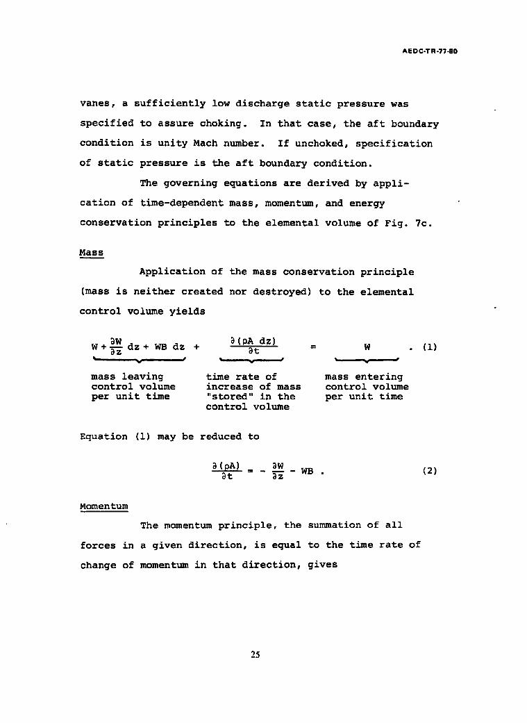
Application of the mass conservation principle
(mass is neither created nor destroyed) to the elemental
control volume yields
BW B(DA dz) W+~ dz + WB dz + Bt = W Q
mass leaving time rate of mass entering control volume increase of mass control volume per unit time "stored" in the per unit time
control volume
(1)
Equation (1) may be reduced to
B(pA) = BW WB . ~t BZ
(2)
Momentum
The momentum principle, the summation of all
forces in a given direction, is equal to the time rate of
change of momentum in that direction, gives
25
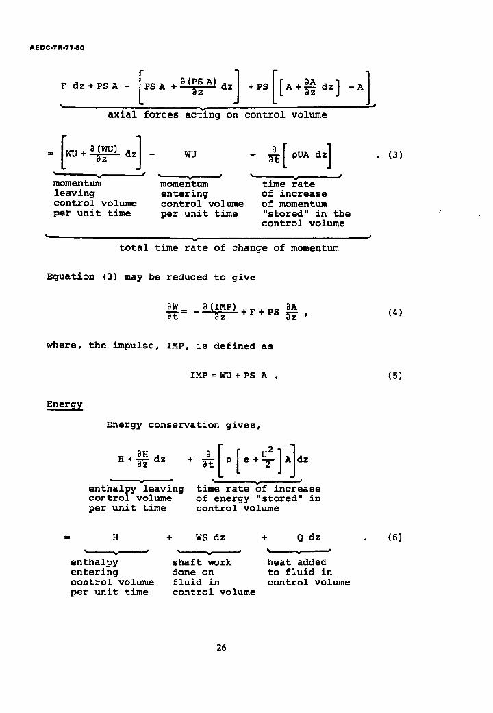
AEDC-TR-77-80
F dz + P S A - P S A + ~(PS~zA) dz + P S A + ~ - ~ dz - A
axial forces acting " on control volume
wu a[wu) z] = +~--~----d - WU
morn en tu~ momentum leaving entering control volume control volume per unit time per unit time
+
time {ate of increase of momentum "stored" in the control volume
total time rate of change of momentum
(3)
Equation (3) may be reduced to give
~W 8(IMP) +F+PS ~A ~-~-- - ~z ~ '
(4)
where, the impulse, IMP, is defined as
IMP =WU+PS A . (5)
Energy
Energy conservation gives,
~H H+~ dz
enthalpy leaving control volume per unit time
+ ~t P ~- dz
time rate of increase of energy "stored" in control volume
= H
enthalpy entering control volume per unit time
+ WS dz + Q dz
shaft work heat added done on to fluid in fluid in control volume control volume
(6)
26
AEDC-TR-77-80
Equation (6) may be reduced to
where
a n d
(XA) _ ~t
~H ~-~+WS +Q , (7)
[ u2] X:p e+-f (8)
H = Cp WT . (9)
State and Additional Equations
Additional equations required include the perfect
gas equation of state,
PS = D R TS , (i0)
calorically perfect internal energy and enthalpy relation-
ships,
e=c v TS +constant , (11)
h = Cp TS + constant , (12)
stagnation (total) state temperature,
U 2 T=Cp TS +-~- , (13)
and stagnation (total) state pressure,
Y
, (14)
27
A E D C-T R -77 -80
where
7=cP CV °
Also required is the Mach number,
(15)
U M = -- (16) a r
where the acoustic velocity, a, is
a = ~7 R TS = ~y ~ , (17)
and the Mach number-static pressure form of the energy in
the control volume,
which results from combination of Eqs. (8), (10), (11),
(15), (16), and (17).
The Mach number-static pressure form of the
impulse, IMP, is also used,
IMP=PS A[I+TM 2] .
(18)
(19)
This equation results from combination of
W=pAU , (20)
with Eqs. (5) and (17).
28
A E D C-T R-77-80
II. STAGE FORCES AND SHAFT WORK
Steady-State Sta@e Characteristics
Consider the element of fluid contained between
two blades in a rotor as shown in Fig. 8a. Entering the
rotor, the tangential velocity is V 8 , and at the exit it is 1
V82. Applying the conservation of angular momentum
principle to the fluid element in steady flow gives the
t=W[r2 V8 -r I ] • 2 VSl
torque on the element,
(21)
Multiplying Eq. (21) by rotor speed, ~, yields the time rate
of doing work on the fluid, which is equal to the total
enthalpy change across the rotor. Thus,
o~ [, ,i [r r ] W - = ~W V@2 V@2 (22)
Replacing the difference between radius-velocity products
using an effective radius yields,
opwE,2 ,l~ o~[vo2 vol]
= -r 1 r2 V82 V81
V82 -V@I
where
(23)
(24)
29
A EDC-TR-77-80
Writing wheel speed as
and
Uwh = ~r ( 2 5 )
gives
- = AV 8 (26) V82 V81
T 2 -T 1 = Uwh AV 8 •
T 1 Cp T 1 (27)
Applying the linear momentum equation for steady
flow to the element of Fig. 8a gives
F 8 =W AVe =Pl A1 U 6V 8 , (28)
where F 8 is the force being applied to the fluid by the
blading in the compressor.
The force, F8, can also be expressed in terms of
blade lift and drag, as indicated in Fig. 8b,
F 8 =L cos(e+k) + D sin(e+A) , (29}
where u is the blade angle of attack, determined by the
velocity triangle of Fig. 8b, and X is the blade chord-to-
axial direction angle, or, the cascade stagger angle.
30

AEDC-TR-77-80
ficients,
and
The lift and drag may be expressed as coef-
L C£ =i V 2 ' (30)
Pl rel Aref
D Cd = 1 Pl V2 tel Aref
(31)
Combining Eqs. (27) through (31) produces
• 1" 2 - T 1
T 1
[ 1 A__~f] Uwh~rel [ ] (32)
Returning once more to Fig. 8b, define the stage flow
coefficient as
U --- . (33}
V e
From Fig. 8b, the flow coefficient, %, is related
to the blade angle of attack, u, by the stagger angle, A,
which is a constant for any given blade row,
¢ = cot(A+a) . (34)
Thus, ~ serves the same purpose in the compressor as ~ does
for aircraft wing aerodynamics. It decreases with
increasing u; therefore, small ¢ means large a, and vice
versa. Also from Fig. 8b,
31
AEDC-TR-77-80
U - - = c o s ( X + ~ ) Vrel
(35)
Combining Eqs. (32) through (35) yields
% ~-i i~ u 2 v 2
T 1
(36)
The left-hand side of Eq. (36) is defined as the stage
loading parameter, #T (following Horlock [20]), or simply as
the stage temperature coefficient (more common in American
works [40]). Thus,
~T = cp(TR-I) ,
U 2 wh T 1
(37)
where TR is the stage total temperature ratio.
If the swirl component of tangential velocity is
smal i,
and
U = - (38)
Uwh
= 2 A 1 + 1 C£ + ( 3 9 )
32
AE 0C-TR.77-80
At given Mach and Reynolds numbers, C£ and C d are functions
of u; thus, #, only. Therefore,
~T I = T(#) . (40) Re,M
In principle, theoretical or experimental lift and
drag coefficients could be used, along with stage geometry,
(A, AI, Are f) to compute the stage temperature coefficients
following Eqs. (36) or (39). Corrections for blade row
interference causing losses and secondary flows would be
required. Another method is to measure the stage total
temperature, flow rate, total pressure, and flow angularity
at the stage entry and exit and directly compute ~T and
from Eqs. (37) and (38). The stage characteristics used in
this study were obtained in that manner and are summarized
in Appendix B.
The temperature ratio of Eq. (37) for an ideal
compressor stage is the isentropic temperature ratio defined
from stage entry and exit stagnation pressure. Using this
ratio, another stage parameter, the stage pressure coef-
ficient, ~P, is produced,
~-__!i
2 Uwh
T 1
(41)
33
AE DC-TR-77-80
The pressure coefficient is also a function of the flow
coefficient, ~, in a manner similar to the temperature
coefficient. The stage adiabatic efficiency is
had = Ahisentropic = PR 7 -1
Ahactual TR-I (42)
Thus,
~P ~ad = V "
(43)
A set of curves,
CT = %T (¢)
I i
~ad = had (~) I J
, (44)
is referred to as stage characteristics, and along with flow
direction,
[%]. (45)
or an equivalent set of flow direction information, fully
defines a stage's performance from a one-dimensional stand-
point. Note that the set of Eq. (44) is redundant; any two
of the three variables are sufficient to compute the third.
Various forms of the stage characteristics are
used. An alternate form used in NACA compressor research,
34
AEDC-TR-77-80
and used for the stage characteristics of the NACA-8 com-
pressor treated in this study, is the equivalent temperature
and pressure ratio form. They are defined as
LCp T J design
EPR = ~P + 1 , (47) LCp T J design
and had is defined as in Eq. (43).
Because
CpTJ design
is a constant for a given compressor, the set remains a
function of ~, as in Eq. (44), and contains the same
information.
Figure 9 is an example set of stage character-
istics for the first stage of the NACA-8 compressor [46].
To the right of the equivalent pressure ratio peak, the
stage is unstalled (i.e., high ~ and low ~). To the left,
the stage is stalled. Rapid decrease of stage efficiency at
low ~ (high u) where the blades are stalled, is evident.
The data of Fig. 9 is seen to generalize well with the flow
coefficient, ~, computed as in Eq. (38) with the swirl
component of velocity ignored. This implies that for this
set of data, the swirl velocity component was either small
35
AE DC-TR-7740
relative to wheel speed, or, changed little as a fraction of
wheel speed over the range of compressor operation con-
sidered. Steady-state stage characteristics for the three
compressors treated in this study were obtained from [43,
46, 47], and are shown in Appendix B.
The foregoing discussion pertains primarily to the
compressor rotor which imparts the shaft work to the fluid.
No stagnation temperature change occurs across the stators
(with adiabatic boundaries) and the stagnation pressure
losses of the stator may be combined with the change across
the rotor to give a net change. Therefore, the character-
istics of Eq. (44) may be attributed to the overall stage.
Unsteady Cascade Effects
When the angle of attack of the flow into the
compressor stage varies slowly, the lift coefficient follows
the steady-state C£-u curve very closely, as illustrated in
Fig. I0. Similarly, the steady-state ~-~ characteristics
are followed. When ~ rapidly changes, however, the lift
cannot instantaneously follow because a certain amount of
time is required for the flow around the blade to adjust to
the new condition. Lag loops or hysteresis in the CE-~ and
~-~ curves appear (Fig. 10).
Goethert and Reddy analyzed the unsteady cascade
effects [32]. They analyzed unsteady incompressible
potential flow through a stationary cascade of thin, flat
plate foils with small oscillations in the axial velocity
36
AEDC-TR-77-80
producing angle-of-attack oscillations. The time-averaged
angle of attack was zero. Their results are summarized in
Fig. ii. The cascade stagger angle is A; the blade chord
length, C; and spacing is a. Rotor speed, ~, was constant
and Vsw was zero. The axial velocity, U, was oscillated at
frequency f, causing an inverse oscillation of ~. This
produced an oscillation in the lift coefficient. The
results were presented in terms of maximum amplitude ratio
at a given frequency, divided by the lift coefficient
amplitude at f = 0 (quasi-steady-state). The resulting lift
ratio is presented as a function of reduced frequency, k,
for four values of cascade spacing, a/C. The case of
a/C = =, a single, isolated airfoil, is shown for reference.
Also treated for reference was the case of oscillating foils
in a steady stream. The Goethert-Reddy work showed signifi-
cant differences to exist between the oscillating foils,
stationary stream, and the converse case. Their work also
showed the unsteady effects for a cascade of finite spacing
to be much less severe than that of an isolated airfoil.
The unsteady influence was shown to increase with increasing
spacing (a/C) and stagger angle, A.
The lift coefficient ratio variation with reduced
frequency is intuitively correct at k = 0 and as k ~ ~.
Following Goethert and Reddy [32] the reduced frequency, k,
may be viewed as an indication of the ratio of flow passage
time to the disturbance stay time of the forced oscillation.
37
A E DC-TR -77-80
The passage time is defined as the time required for an air
particle to pass through the blade row channel. Or,
_ C ( 4 8 ) Atpassage Vre I "
The disturbance stay time is defined as the time that any
one blade is exposed to the positive disturbance velocity of
one velocity oscillation, that is,
Therefore,
1 Atdisturbance = 2-~ " (49)
dt~assa~e = 2f___.~C=
Atdisturbance Vrel (50)
Alternately, k may be viewed as being proportional
to the ratio of the blade chord length to the disturbance
wave length,
chord length _ C _ Cf _ k wave length Vrel Vrel ~-~ . (51)
If k is near zero (i.e., the disturbance time period is
large compared to the passage time), the blade lift will
easily follow the disturbance. Similarly, the chord length
is small relative to the disturbance wave length; thus, the
lift can easily respond. If k * ®, the disturbance time is
small compared to the passage time and many disturbance wave
38

A E D C-T R-77-80
lengths reside within one chord length at any instant in
time. The disturbance is then "averaged-out" by the blade
yielding an instantaneous lift value of zero due to the
disturbance.
Bruce and Henderson [48] conducted an experi-
mental investigation of the unsteady force coefficients
produced by a compressor rotor in unsteady flow. A single
stage, low-speed compressor was fitted with a rotor blade
having a segment of the blade on a small strain-gaged force
balance. This installation allowed a direct measurement of
the unsteady forces acting on that blade segment as the
rotor passed through a distorted flow field produced by a
distortion screen. A portion of their measurements was
taken with stagger angle and cascade spacing near the values
used by Goethert and Reddy. Figure 12 shows a comparison of
the Goethert-Reddy analysis with the Bruce-Henderson experi-
mental results. The trends with reduced frequency are in
good agreement. The experimental results generally were
from I0 to 20% higher than the analytical results. Con-
sidering the difficulties and assumptions involved in both
the analytical and experimental evaluations, this level of
agreement is considered reasonable at this time. Agreement
among other theoretical treatments and experimental results
surveyed was usually of this order or worse. (See compari-
sons made in [48] for example.)
The analysis of Goethert and Reddy was performed
for an unloaded cascade, that is, the mean angle of attack
39
AE D C-T R-77-80
was zero. Figure 13 shows the variation of lift coefficient
ratio with mean angle of attack from the unsteady cascade
work of Ostdiek [49], and Bruce and Henderson's single-stage
compressor [48]. The dynamic lift coefficient ratio magni-
tudes were normalized by the value of a mean angle of attack
of eight degrees. The measurements were made over a range
of reduced frequency of 0.002 to 2.9, and from 0 to 12
degrees mean angle of attack. The results are all within
±10% and no generalized trend could be identified.
Unstead~ Stave Characteristic Correction
The Goethert-Reddy analysis may be used to con-
struct a correction to the steady-state stage character-
istics. To facilitate application of the correction, the
dynamic lift coefficient ratio was represented by a simple,
first-order differential'equation, as indicated in Fig. 14.
The equation,
dC£ C£ C£s s + - (52) T T '
represents the time-dependent lift coefficient, C£, in
response to the quasi-steady-state lift coefficient, C£ss,
which would be produced if the lift exactly followed the
steady-state C£-~ relationship.
The blade time constant, T, depends on the chord
length and reduced frequency,
40
A E DC-T R-77-80
EC "[ - • (53)
Vrel
The constant, E, depends on cascade geometry (i.e., a/C and
A). For a/C = 1.0, and ~ = 50 degrees, £ = 0.3106. The
value of E is found by fitting the approximating differ-
ential equation, Eq. (52), to the response indicated by the
Goethert-Reddy analysis.
For sinusoidal variation of angle of attack, the
amplitude response of Eq. (52) is
IC~Imax I , = 1
Ic~ls~ + (~ ~) . (54)
The approximation of Eq. (52) is compared to the Goethert-
Reddy solution in Fig. 14, and fidelity .is excellent up to
k=8.
The cascade airfoil lift coefficient is related to
the stage characteristics through Eq. (39). Consider
oscillations of the flow into a stage around a given stage
characteristic operating point (~o' ~o )" Let ~ represent
either ~T or ~P. Expanding Eq. (39) in a Taylor series,
neglecting the drag coefficient term and retaining only the
first-order terms of the series gives
11'2 ~" A 1
(55)
4]
AEOC-TR-77-80
Near the point, (~o' ~o )'
- ~O
- ~o 0
(56)
Then, from Eqs. (55) and (56),
'to -1
Are f 1/2 - ] . (571
Substituting Eq. (57) into Eq. (52) produces,
d~ ~ ~ss EE + E = - E - • (58)
Thus, the stage characteristics may be corrected for
unsteady cascade airfoil influences using the same first-
order differential equation algorithm as that constructed
for the unsteady lift coefficient.
The linearization of the unsteady correction
implicit in Eqs. (55) and (56) is justified by: i) the
Goethert-Reddy analysis is itself a linearized analysis;
2) the correction magnitude is small in the range of reduced
frequency normally encountered, as will be demonstrated
later. The correction is actually proper only up to the
stall point (i.e., up to the point where unsteady viscous
effects become predominant).
42
AEOC-TR -77-80
Force and Shaft Work Distributions
The momentum equation, Eq. (4), requires an axial
force distribution representing the force of the compressor
blading and casings on the fluid. The function is con-
structed from the experimentally determined steady-state
stage characteristics corrected for unsteady effects. (Or,
alternately, the force may be computed in a quasi-steady-
state manner from the steady-state stage characteristics and
then directly corrected for unsteady effects using the
dynamic lift coefficient ratio of Fig. 14.) The shaft work
distribution required by the energy equation, Eq. (7), is
similarly constructed.
The exact method of extracting the force and shaft
work distributions depends partly on the finite difference
method used to solve the governing equations, and is
described in the next section.
Ill. METHOD OF SOLUTION
The basic governing equations are:
(~A) ~W ~----~ = ~z WB , (2)
and
~W _ 3 (IMP) + F + PS 5A 9t ~z B--{ , (4)
(XA) _ ~H Bt ~z + WS + Q . (7)
43
AEDC-T FI-77.80
The dependent variables to be integrated for are pA, W, and
XA. The area, A, was preserved in the derivative to allow
for cases where exit area is rapidly changed.
Finite Difference Approximation, One-Sided
Difference Form
The spatial derivatives were approximated in two
different finite difference forms. When only the compressor
was considered Ino ducting), a simple, one-sided difference
approximation was used. The control volume was divided into
unequal lengths. Each length included a stage of the com-
pressor as shown in Fig. 15. Figure 15 also shows the
computation plane designations. The spatial derivatives at
location i were approximated by
aw. w. - w. i ~ 1 im
-~z zi _ Zi m , 1591
a (IMP) i
az
~ IMPip - IMP i
Zip - z i , (60)
aA. 1
-~ = constant , 161)
(the product of static pressure with the area-derivative was
combined with the force term, F),
and
aH i H i - Him m
-~z z. - Z. " (62) 1 im
44
A E DC-TR-77-80
Substitution into Eqs. (2), (4), and (7) produces
the approximate equations,
~(PA)ip = Wi - Wip
8t Zip - z i ' (63)
and
~w. IMP. - IMP.
_ i ~ P + F~ (64) -~t z. - z. J. ap i
(XA) . H. - H. ip = i ip + WS. + Qi (65)
~t z. - z. 1 " ~p
Writing Eqs. (63), (64), and (65) from i = 1 to
i = in-l; that is, from the forward to the aft control
volume boundaries, results in 3x(in-l) first-order differ-
ential equations to be solved simultaneously.
Force and Shaft Work Computation
The division of the control volume into stage
lengths was made because the forces and shaft work applied
between stage entry and exit are obtainable from the stage
characteristics. To determine the force and shaft work
applied to each element, the flow coefficient into the
element is calculated,
U • = 1
~i ~ . (66)
1
45
AEDC-TR-77-80
The stage characteristic, represented as a polynomial curve
T (or n i) are found. fit, is then entered and ~ and ~i
Corrections for unsteady effects are made. The stage stag-
nation pressure ratio and temperature ratios which go into
the force and shaft work computations are calculated from
a n d
wh P PR i = = 1 + c~ ~i (67)
wh T TR i = = 1 +c~ ~i "
Shaft work is computed as
WSi = WiTi[ TR i - i] .
Similarly, the axial force is given by
(68)
(69)
= IMP [IMPR. - 1] (70) Fi i I "
IMPR i is the impulse function ratio across the stage,
determined from the stagnation temperature and pressure
ratios, area ratio, and flow directions,
Y
46
AE D C-T R-77-80
The variable, ME, is the equivalent Mach number downstream
of the stage which would be present if steady flow existed.
(Recall that the stage characteristics from which the forces
and shaft work are determined, are based on experimental
steady-state measurements). The value of ME is computed
from a polynomial expression approximating the inverse of
Eq. (72), for constant R and 7,
r- +ll I y---l-I
(72)
MFFE is the downstream equivalent mass flow function,
w VT i TR i MFFE = i (73)
Pi PRi Aip cos Bip '
defined in the same spirit as was ME.
The flow direction angles, ~i and Sip, taken with
respect to the axial direction, are input as functions of
compressor corrected rotor speed, as constants, or, are
assumed to be zero if no flow direction information is
available.
Solution Procedure
Figure 16 outlines the overall digital computer
solution procedure followed. The problem is solved as an
initial condition problem. Following the flow path of
Fig. 16, at time equal zero, initial values of the dependent
47
AEDC-TR-77-80
variables are specified. Entry plane, interior plane and
exit plane conditions along with forces and shaft work are
computed for time equal zero and are used to compute the
time derivatives of the dependent variables. The time
derivatives are then integrated using a fourth-order Runge-
Kutta numerical integration method [50] for the dependent
variabie values at the next step in time. The new values
are then used to compute conditions for that time step and
the solution advances in time until the desired solution is
obtained.
Some additional details of the computation pro-
cedure are as follows.
Entry plane conditions. At the forward boundary,
i = 1, flow, Wl, will be available from integration of
Eq. (64). Density, PI' and the energy variable, Xl, are
not available and must be supplied by the boundary condition.
Stagnation pressure, PI' and stagnation temperature, TI, are
supplied as boundary conditions. The mass flow function,
is computed.
function by
wi 7 MFFi = PIA1 ' (74)
Mach number is related to the mass flow
y--rlj (75)
48
AE D C-T R-77-80
The inverse form of Eq. (75) is approximated by a polynomial
curve-fit of M 1 as a function of MFF 1 for constant R and 7.
Static temperature, static pressure, density, and the energy
variable may be computed knowing Mach number:
-1
[ Tsz ] PSz = PI L ~?z J
(76)
, (77)
and
PS 1
Pl - R TS 1 '
Psl[ 21 X 1 = ~-~ 1 + ~ M 1 .
(78)
(79)
Interior plane values. On the interior planes,
values of the three dependent variables are known from
integration. To provide the other variables necessary for
the solution, the following calculations are made at each
W, 1
Ui = pi-~--~i '
plane:
(80)
_ 1[xi TSi Cv Pi -~ ' (81)
PSi = Pi R TS i , (82)
49
AEDC-TR-77-80
u 2
T i = Cp TS i + ~ , (83)
Pi = PSi T~ i
7
, (84)
a i = ~7 R TS i , (85)
and
U, M. - 1 1 a i '
IMPi = PSi Ai[l + 7 M2]z
(86)
, (8";)
H z. = Cp W.~ T i . (88)
Exit plane values. Density, p, and the energy
variable, X, are available from integration. Flow, W, is
not available from integration and must be found using the
aft boundary condition. At the exit plane of the aft
control volume, static pressure is specified. Exit
stagnation-to-static pressure ratio is tested against
critical pressure ratio to determine if the exit is choked
or not, as follows:
7
[ ]ori. (89)
50
AEDC-TR-77-80
If
[P] Pxn • ~
Pexit -- crit
the exit is choked and
Min = 1.0 .
Then,
If
(7-1) Xin PS. =
~n i + 7(7-1) " 2
(90)
Pexit crit
the exit is unchoked, and
PSin = Pexit "
Therefore,
q[ 2 Min =
Xin 1 ]
PSin 7-i (91)
Mach number and static pressure are now known for either
condition. Therefore, the remaining calculations are conuoon
for either case.
5]
AED C-TR-77-80
and
PS. in TS. -
in R -1°-n ' (92)
Uin = Min ~ 7 R TSin , (93)
Win = Pin Uin Aexit " (94)
Impulse and enthalpy values at the exit and entry
planes are computed using Eqs. (87) and (88).
Finite Difference Approximation, Central
Difference Form
When ducting ahead of and behind the compressor
was included in the system modeled, a noncentered, two-sided
difference form of finite difference approximation was used
to allow more accurate representation of the duct flow
processes and to avoid some numerical stability difficulties
experienced in attempts to apply the one-sided difference
form to duct-flow cases.
The central difference algorithm used is derived
as follows. Let y(z) be any variable with continuous third
derivative with respect to z, for which an approximation to
o~z desired. Referring to Fig. 15, let is
and
~Zip = Zip - z i ,
dZim = Zim - z i •
(95)
(96)
52
AEDC-T R-77-80
Expanding around the i th location,
a n d
i
.~j. . ~I .:°.0[.:.] Yim = Yi 8z AZim + 2 8z 2 li
(97)
(98)
Multiplying Eq. (97) by AZ~m, Eq. (98) by AZ~p, differencing the results and solving for ~-~zli gives
where
~z] -a +a.,.+ -0[~z'] i im Yim aip Yip
Az=max [AZip , AZim] ,
and the weighting terms are
• (99)
(100)
and
AZ. a. = ip
am Az. am AZip - AZim ]
a i = -
dZim + ~Zip AZip dZim
AZ. am 1 aip'~zip [~,io_~zip]
I (i01)
53
AEDC-TR-77-80
The sum of the coefficients,
aim + a i + aip 0 (102)
Multiplying Eq. (102) by Yi and subtracting from Eq. (99)
gives
(lO3)
Replacing the spatial derivatives in the governing
equations, Eqs. (2), (4), and (7), produces the alternate
finite difference form,
~[~,]~ "i~[ ~ -,~ip ] - ~ , (104)
~W.
@= aim [ IMP i - IMPim] + alp [ IMP i - IMPip ]
and
~A +F+PS. 0
i (105)
~[~,]~ ~ ° o~ [ ~ - ~ ] * ~ [ " ~ - . ~ ] . ~ . o . (106)
As was done with the one-sided case, the pressure-area
partial derivative in Eq. (105) was combined with the axial
force term.
54

A E D C-T R-77 -80
The solution procedure followed (Fig. 16) was the
same as used in the one-sided case except Eqs. (104), (105),
and (106) were used instead of Eqs. (63), (64), and (65).
The bleed flow, forces, shaft work and heat added
must also be made compatible with the two-sided difference
form. Thus,
and
WB = aim WBim -aip WB i , (107)
F= -aim Fim+aip F i , (108)
WS= -aim WSim+aip WS i , (109)
Q = - aim Aim + aip Qi " (110)
Also, on the forward and aft boundary planes, an appropriate
one-sided form of the differential equation was used. The
force term for ducting was taken as a simple friction loss
expressed as
F i = -Cd. 7 PS i A i M~I " (iii) 1
The value of Cd. was adjusted to give a reasonable stag- 1
nation pressure loss in the ducting and to permit
numerically stable operation of the model.
55
AEDC-TR-77-80
Interpretation and Limitations of
Differencin~ Methods
Differencin~ al@orithm truncation error. The one-
sided algorithm is a first-order approximation (i.e., it
ignores terms of order (~z) and above). The central differ-
ence algorithm is a second-order approximation (terms of
order (dz) 2 and above are ignored).
Let y again be any variable in the problem
requiring spatial differentiation. The one-sided algorithm
is found from expansion around a point,
i x 2 ~z2 i (112)
Solving for the first partial derivative,
i
(113)
The truncation error in the governing equations is the error
resulting from the substitution of the algorithm for the
exact form of the spatial partial derivative. Therefore, an
upper estimate for the truncation error for the one-sided
case is
1 ~2y, ~ -- ~- ~-~-~-! (~z) .
oZ 'i (114)
56
A E D C-T R -77 -80
The second partial derivative is finite, so, as Az -7 0, the
error vanishes and, referring to Eq. (112), the approxi-
mation is consistent of order one.
A similar analysis of truncation error for the
central difference algorithm produces an error estimate of
E ~ ~ (nz) .
~z i
(ll5)
The central difference algorithm is therefore consistent of
order two.
For the problems solved using the nonlinear
system of equations produced by the approximation, numerical
stability was investigated by running various time step
sizes and observing the behavior of the solution at large
times.
The system of equations constituting the model is
for time-dependent, one-dimensional subsonic flow and is
hyperbolic in nature, with specified boundary conditions and
initial conditions. Thus, each integration step to compute
the dependent variables at the new time, (t + At), must be
made within the region of influence of the known values at
time, t. The Courant-Friedrichs-Lewy maximum time step
criteria [51],
dZmin (116) Atmax - a + Uma X '
57
A E DC-TFI-?7-80
must be observed. For AZmi n = 0.25 ft, a = 1553 ft/sec
(value at TS = 1000aR), Uma x = a,
At = 8x10 5 sec . max
Values used were typically one-half of dtma x. Various
values, depending on the nature of the specific analysis,
were used.
With consistency and numerical stability, con-
vergence is implied [51]. The best proof of convergence of
the numerical solution is provided by the comparisons to
experimental results given in Chapter III.
Disturbance fre~uenc~ limitations. The differ-
encing length is Az; therefore, no disturbances having
disturbance wave lengths of order Az or less can be
explicitly treated by the model. As a working limit,
minimum wave lengths were restricted to i0 AZma x. There-
fore, the highest frequency phenomena with downstream
propagation of pressure disturbances which could be
explicitly treated by the model would be
(U + a)mi n = , (117)
fmax 10 AZma x
where U is a representative minimum axial velocity, and a is
the acoustic velocity. For U = 300 ft/sec, a = 1116 ft/sec,
and AZma x = 0.25 ft,
58
A E D C-T R -77-80
f = 566 Hz . max
Similar limits can be computed for temperature rather than
pressure oriented disturbances.
Steady-state solution. Inspection of the approxi-
mating equations, Eqs. (63), (64), and (65), or Eqs. (104),
(105), and (106), shows that when the time derivatives are
zero, the remaining equations are the exact mass, momentum
and energy equations for steady, one-dimensional flow
through a control volume of any specified size. The
governing equations in the approximate form could also have
been derived from an integral analysis of time-unsteady flow
through a finite control volume.
59
AEDC-TR-77-80
CHAPTER III
EXAMPLE PROBLEMS WITH COMPARISON TO EXPERIMENTS,
ONE-DIMENSIONAL MODEL
Three steady-state examples and three dynamic
examples are given. Three different compressors, the
Allison XC-I, the NACA-8, and the General Electric J85-13,
were driven to their stability limit for steady flow to
demonstrate the physical processes and to test the models'
ability to compute the steady-state stability limit. The
NACA-8 compressor was stalled dynamically by imposed
oscillating inflow. Dynamic response of the J85-13 for
first oscillating inflow and then for oscillating back
pressure was computed. Finally, the response of the NACA-8
compressor to a rapid inlet temperature ramp representing
rocket exhaust gas ingestion is presented.
Three different compressors were modeled because
experimental data necessary for comparison to the analytical
model did not exist in a sufficiently complete set for any
single compressor. A side benefit of modeling three com-
pressors is the demonstration of the generality of the
analysis method.
50
A E D C-T R-77-80
I. STEADY-STATE STABILITY LIMITS
The Allison XC-I compressor is a four-stage
compressor with design airflow and stall pressure ratio of
38.7 lbm/sec and 4.9:1. Details of the compressor, the
overall compressor map, and the stage characteristics used
in the model are presented in Appendix B. The information
on this compressor was taken from [43]. The computational
stations for the model are shown in Fig. 17a. No ducting
was included in this model, thus, the one-sided difference
formulation was used.
The compressor was loaded to the stability limit
by increasing the exit pressure until flow breakdown was
indicated. Inlet stagnation pressure and temperature were
constant. Corrected rotor speed was 90% of design.
Figure 18 illustrates the loading and the resulting stall
process. Exit static pressure was ramped at a rapid rate to
minimize computer time necessary for the computations. The
rate was sufficiently slow, however, that transient effects
were very small. Airflow at any stage never differed from
compressor inlet airflow by more than 0.5% during loading.
As the load on the compressor increased, compressor pressure
ratio increased and airflow decreased until flow breakdown
was indicated. Figure 19 shows some key compressor
variables on an expanded time scale covering the flow break-
down as computed by the model. Stage 3 flow coefficient
reaches its stall value at t = 55.7 msec. The flow, W3,
61
A E D C-T F1-77 -80
into stage 3 is seen to begin to decrease at the same time.
Shortly afterward the flows at each location begin to
diverge one fr~n the other and to oscillate. The static
pressure behind stage 3 rapidly falls because the stage's
pumping capacity is quite limited when stalled. The
pressure forward of stage 3 rapidly increases in response to
the sudden blockage to the flow which the stalled stage 3
produced. This static pressure signature is observed
experimentally, and is a common means employed to determine
which stage in a compressor stalled first, causing the
instability to occur. (See Fig. X-27 in [14] for example.)
Figure 20 shows the 90% corrected rotor speed
characteristic computed from the model compared to experi-
mental measurements. The flow breakdown point indicated by
the model agreed well with the experimental stability limit.
The model solution thus indicates the following
sequence leading to compressor instability. The compressor
is loaded and flow reduces until a stage somewhere in the
compressor reaches its stall point (its maximum pressure
coefficient point). The ability of that stage to continue
to pump flow (i.e., to help support the pressure gradient
over the length of the compressor imposed by the back
pressure load) begins to diminish. As the flow reduction
because of the increasing load continues, the ability of the
stage to pump diminishes even further because of the
increased load. Eventually, a point is reached where the
flow into the stage becomes fully stalled, thus, little
62
A E DC-T R -77-80
force on the fluid is provided to pump the flow, and the
flow path through the compressor becomes blocked because of
the highly separated condition of the stalled flow in the
channels. In terms of the solution of the model equations,
as the loading is increased, a point is reached where no
stable solution to the governing equations exists which will
satisfy the imposed load (boundary conditions); thus, the
solution, like the flow through the compressor, becomes
unstable. However, the behavior of the model quickly
becomes nonrepresentative of the compressor shortly after
flow breakdown because the stage characteristics are not
valid for deeply stalled, dynamic situations.
NACA-8 Compressor
The NACA-8 compressor is an eight-stage com-
pressor with design airflow and stall pressure ratio of
65 lbm/sec a~d 10:1. Compressor details and stage charac-
teristics are given in Appendix B and are taken from [44,
45, 46]. The model included inlet ducting and combustor
ducting, thus, the central difference form was used.
Computation planes are shown in ~ig. 17b. Figure 21
illustrates the loading of the NACA-8 model to the stability
limit by reducing the turbine nozzle area. The nozzle was
choked. Corrected rotor speed was 90% of design, inlet
stagnation pressure and temperature were constant. Pressure
ratio increased and corrected airflow decreased until
instability was encountered. The process was repeated at
63
AE DC-TR-77-80
70 and 80% corrected speed. The results are presented in
Fig. 22 and are compared to experimental data. Reasonable
agreement was obtained.
Extensive internal steady-state experimental
measurements were made on the NACA-8 compressor allowing
detailed model-to-experiment comparisons. Figure 23 shows
the variation of stage flow coefficients near the stability
limit as a function of corrected rotor speed. Both experi-
ment and model computed values are shown. Good agreement
was obtained.
It is also evident from Fig. 23 that this com-
pressor operates with forward stages below the stall value
of stage flow coefficient at corrected rotor speeds below
approximately 78%. Both experimental and computed flow
coefficient values for stage 1 are below stall at 70% speed.
This behavior is in agreement with previous theories and
experiment observations (see Chapter I and [21, 24]). An
explanation is as follows. At low corrected rotor speeds,
the forward stages are unable to deliver the design pressure
ratio. The flow density provided to the aft stages is
therefore much lower than that for which the compressor
axial area distribution was designed. Thus, to maintain
steady mass flow continuity, the flow coefficients (axial
velocity) in the aft stages are high. Indeed, at suffi-
ciently low corrected rotor speeds, the aft stages are even
choked. This limits the flow through the compressor to a
low value. It also means that the aft stage characteristics
64

A E DC-T R-77-80
will be steep relative to the forward stages (see Appendix
B). Therefore, at low corrected rotor speeds, as the load
on the compressor (the demanded pressure ratio) is increased,
flow reduces, and the following sequence occurs. The
ability of the aft stages to increase their pressure ratio
in response to the flow reduction is initially greater than
the decrease in pressure ratio occurring in the forward
stages in response to the same reduction in flow rate. Thus,
the increased load may be satisfied. As the loading con-
tinues, however, the forward stages become more and more
stalled, and a point is eventually reached where the aft
stages can no longer compensate. At that point, the load
can no longer be satisfied, and overall compressor insta-
bility occurs.
This example makes clear the need to distinguish
between stage stalling and overall compressor stalling or
instability. Overall compressor instability is always
preceded by stage stall, but is not always simultaneous with
stage stall.
General Electric J85-13 Compressor
The General Electric J85-13 compressor is an
eight-stage compressor with design airflow and stall
pressure ratio of 43 ibm/sec and 7.7:1. The compressor
employs a set of variable inlet guide vanes ahead of the
first-stage and compressor bleed from the second-, third-,
and fourth-stage stator cases. The guide vanes and bleed
65
AE DC-TR-77-80
valve are scheduled by the engine control as functions of
corrected rotor speed. (Additional bias for inlet tempera-
ture is also sometimes provided.) The schedules used in the
model of this study are given in Appendix B. Stage charac-
teristics and additional compressor details are also given
in Appendix B and are taken from [47].
The steady-state stability limit and corrected
speed characteristics were computed for 80 and 87% corrected
rotor speed and are compared to experimental results
(Fig. 24). Agreement was good. The compressor model was
loaded by reducing turbine nozzle area. The nozzle was
choked. The model included ducting, thus the central
difference formulation was used.
II. DYNAMIC STABILITY LIMITS
Oscillatin~ Inflow Loading, NACA-8 Compressor
Figure 25a shows the oscillation of the inlet
total pressure imposed on the NACA-8 compressor model.
Inlet total temperature and turbine nozzle area were
constant. Corrected rotor speed was 70%. The pressure was
oscillated at 20 Hz and the amplitude was slowly increased
until compressor instability occurred. Overall compressor
pressure ratio responded as shown in Fig. 25b. For con-
venience, the model was started at 90% speed (initial
conditions were previously calculated for 90% speed),
rapidly decelerated to 70% speed, stabilized, and then the
oscillation was imposed at t = 0.15 second.
66
AED C-TR-77-80
The pressure ratio oscillations grew with the
imposed pressure oscillations until instability was
encountered. The response of the airflow into the com-
pressor is shown in Fig. 25c. Initially, the flow variation
is near sinusoidal, but, as the stages are driven into and
out of their stalled regions, indications of flow breakdown
begin to appear. Finally, the flow completely diverges to
zero. The phase shifts and amplitude variations of the flow
properties through the compressor due to the forced oscil-
lations cause the stage flow coefficients to oscillate.
Figures 25d through 25g show the flow coefficient dynamic
variations. Also indicated are the individual stage stall
values and the value of each flow coefficient at which the
compressor steady-state stability limit was reached at 70%
rotor speed. Excursions well below both values occur
dynamically before total flow breakdown is experienced.
This behavior is in qualitative agreement with experimental
observations reported in [5, 37]. Examinations of the flow
coefficient variations indicate that stage 7 was the stage
which eventually became totally unstable and caused com-
pressor instability (Fig. 25g).
Interpretation of the model results suggests the
following physical process for instability with oscillating
inflow. The stage flow coefficients are alternately driven
into and out of their stalled regions. The stages must be
held in the adversely loaded condition for a sufficiently
long period of time for the flow breakdown to occur. Thus,
67
AE DC-TR-77-80
at a given frequency, the amount of time a stage (or group
of stages) will be in the highly loaded condition depends on
the amplitude of the imposed oscillation. Once a stage (or
group of stages) is transiently held in the adversely loaded
condition for a sufficient time period, the breakdown
process is locally like that which occurs in steady-state
loading.
The extent to which the flow coefficients oscil-
late depends on the dynamic response (phase angle and
amplitude ratio), which depends on oscillation frequency.
The loading process of Fig. 25 was repeated for frequencies
up to 320 Hz. The amplitude of imposed oscillation required
to drive the compressor to the stability limit is shown in
Fig. 26. As frequency increases, the amplitude required for
instability decreases. This occurs because, as frequency
increases, the phase lags and amplitude attenuations across
the stages increase; thus, the flow coefficient oscillations
are larger for a given imposed oscillation amplitude at
higher frequencies. (A fundamental discussion of the phase
shift and amplitude ratio effect is given in [24].)
A local minimum occurs in Fig. 26 near 80 Hz.
This occurs because, below 80 Hz, aft stages in the com-
pressor are critical, but, at frequencies higher than 80 Hz,
the amplitude attenuation across the forward stages
increases to the extent that it protects the aft stages, and
a new stage, farther forward in the compressor, becomes
critical.
68
A E D C-T R -77-80
The computations of Fig. 26 were made both with
and without the unsteady cascade correction to the stage
characteristics. First-stage reduced frequency is indicated
at each value of oscillation frequency. Only small
influences were experienced for this compressor in oscil-
latory inflow because of the relatively low reduced
frequencies. Compressors and fans with larger blades would
experience the influence of the correction at somewhat lower
frequencies.
No experimental data were available for this com-
pressor for direct comparison of stability limits. The
general trend with frequency and the amplitude magnitudes
are in agreement with the experiment of [37], however.
Oscillatin~ Inflow D~namic Response,
J85-13 Compressor
As indicated in the previous section, the ability
of the model to properly compute stability limits in oscil-
latory flow depends on its ability to compute the dynamic
response of the various stages in the compressor to the
imposed oscillations. Two experiments were carried out by
NASA using the J85-13 turbojet engine to measure the
unstalled dynamic response of the compressor to imposed
inflow oscillations [52, 53]. Figure 27 is a sketch of the
test arrangements. One test was conducted in a supersonic
wind tunnel with an axisymmetric mixed compression inlet
installed (Fig. 27a). Engine entry total pressure
69
AE DC-T R-77-80
oscillations were produced by oscillating the inlet bypass
doors, causing the terminal normal shock in the inlet to
oscillate, thus producing the downstream total pressure
oscillations. The other test arrangement (Fig. 27b) used an
airjet system in a section of ducting ahead of the engine.
The airjet system operates by blowing high velocity air
counter to the primary airstream. Planar oscillations in
engine entry pressure were produced by oscillating the air-
jet counterflow. In both cases, the oscillation amplitude
was approximately 10%, peak-to-peak.
The J85-13 compressor model was subjected to
imposed total pressure oscillations at the forward control
volume plane, thus simulating the inlet experiment of
Fig. 27a. The test setup of Fig. 27b differs from the model
and the inlet experiment, in that the forward isolation
plane provided by the supersonic flow in the throat of the
inlet is not in the airjet test setup. The inlet and model
dynamic systems consisted of the ducting downstream of the
normal shock wave to the choked turbine nozzle in the engine.
The airier dynamic system includes all of the test cell
ducting forward of the engine (until a choked valve,
venturi, or other forward isolation point is reached) down
to the choked turbine nozzle in the engine.
Figure 28 shows the variation of pressure amplitude
ratio and phase angle for a 40-Hz oscillation through the
compressor. Model computations are compared to the NASA
data. The calculated trends are in good agreement with
70
AE DC-TR-77-80
experiment. Normalized magnitude differs by approximatoly
10~ and phase angle by five degrees. The agreement,
although reasonable for dynamic response data, could be
improved by closer matching of engine operating condition
between model and experiment. Also, the J85-13 engine run
in the wind tunnel was likely not the same engine from which
the stage characteristics were taken; thus, engine-to-engine
variations are present. Further, the measurement uncertain-
ties present in the experimental data (quoted as ±3% on
pressure measurement and ±8 degrees on phase angle in [52])
may affect the comparison.
More detailed dynamic response results are shown
in Fig. 29. Figures 29a and 29b represent the frequency
response across one stage; Figs. 29c and 39d across approxi-
mately half of the compressor; and Figs. 29e and 29f across
the entire compressor. Trend and level agreement between
the model computations and the inlet results were reasonable,
but, once again, could be improved by closer matching of the
actual experimental hardware. In particular, the compressor
discharge agreement suffered because the combustor volume of
the actual engine was larger than that modeled. The com-
bustor in the model was shortened during steady-state
stability studies to keep the number of computation planes
to a minimum, and was not increased for the dynamic response
study.
Comparisons of the model and engine-with-inlet
results with the airier results show considerable
7]
AED C-TR-77-80
differences, especially near 40 Hz. The most likely cause
for the difference is the fact that the two dynamic systems
are not equivalent.
The model configuration used in the computations
was not tailored in detail to the experimental configuration
tested. The comparison shows that to obtain close agreement
dynamically, close attention to matching configuration must
be observed. The comparisons also show that considerable
care must be exercised in dynamic experimental work to
assure dynamic equivalency of systems (e.g., same isolation
points, volumes and geometry).
The results also suggest a potentially powerful
coupling of experimental work and analytical modeling. For
example, if it were not possible (or desired) to physically
dynamically isolate the airjet setup in the test cell to
simulate a given inlet-engine combination, the test setup,
including the airier system and the compressor, could be
modeled and the model refined using experimental results to
closely match the test setup measurements. Then, the
analytical model inlet configuration could be modified to
match any desired configuration, and the desired information
derived from the model.
Oscillatin@ Compressor Discharge Pressure,
J85-13 Compressor
Fuel flow to the J85-13 engine run with the super-
sonic inlet (Fig. 27a) was oscillated to determine the
72
AE DC-TR-77-80
propulsion system's dynamic response to oscillations induced
within the engine. The oscillations produced compressor
discharge oscillations of approximately 10%. The inlet was
assumed to remain started, thus, the model dynamic system
boundaries were the same as for the oscillating inlet bypass
door case. Computations were made using the J85-13 model by
adding heat to the combustor control volumes in an oscil-
latory manner to produce peak-to-peak oscillations in
compressor back pressure of approximately 10%.
Figure 30 provides a comparison between computed
and experimental amplitude ratio and phase angle variation
through the compressor at a frequency of 40 Hz. Trend and
level agreement were reasonable. Because of the high com-
pressor rotor inertia, at 40 Hz, rotor speed cannot respond
to the imposed fuel flow oscillations; thus, the effects of
the oscillation are from aerodynamic upstream propagation
only. The aft-stage characteristics (stages 4 through 8)
(Appendix B) are quite steep, and at this condition, the
stages are operating on the steep, negative slope part of
the curves. Therefore, perturbations in the aft-stage
airflow (or flow coefficient) will cause large oscillations
in stage pressure ratio. Figure 30 indicates the magnifi-
cation of the induced oscillation at the stage 4 entry.
However, stages i, 2, and 3 are operating in the flow coef-
ficient range of 0.5 to 0.55 (i.e., on the shallow, positive
slope part of the curves for stages 2 and 3, and the
shallow, negative slope range for stage 1). As a result,
73
AE DC-TR-7?-80
the forward stages oscillate pressure ratio very little in
response to a given airflow oscillation. Therefore, the
forward stages attenuate the upstream propagating dis-
turbance to the point that it is barely measurable at the
compressor inlet (Fig. 30a). Thus, it becomes clear that
the stage characteristic shapes and match points play a very
important role, not only in the steady-state stability of
the compressor, but also in the way disturbances are propa-
gated, thus, in the transient and dynamic stability
characteristics of the compressor.
Figures 31a and 31b present the dynamic response
to oscillating fuel flow across the compressor. Experi-
mental results are presented along with three different sets
of model computations. The first set is for constant rotor
speed and constant P1 and T I. The second set is for
variable rotor speed and constant P1 and T I. The third set
is for variable rotor speed, variable P1 and constant T I.
The three sets were computed to account for the three
dynamic effects caused by oscillating fuel flow. At fre-
quencies above approximately 20 Hz, the rotor speed cannot
respond to the oscillating fuel flow~ thus, as already
discussed, upstream aerodynamic propagation is the chief
mechanism present. At frequencies below 20 Hz, rotor speed
can respond to the oscillations in fuel flow. thus, the
stage flow coefficients must now vary mechanically also
(i.e., wheel speed oscillates). Further, because wheel
speed varies, compressor airflow demand also must vary.
74
AEDC-TR -77-80
Inlet airflow varies as a result and causes the normal shock
wave to oscillate. This causes the inlet total pressure,
PI' to oscillate.
Engine rotor speed response was represented in the
model by a simple first-order differential equation simu-
lating the engine control and rotor dynamic response. An
oscillation in Pl' at the control volume forward boundary,
was imposed to simulate the shock wave motion. As seen in
Fig. 31, reasonable agreement with experiments was obtained
only when all three of these effects were included. Because
of the complicated nature of the three disturbance paths,
agreement between model computations and experimental
results at internal compressor locations was poor. Agree-
ment could be improved by more exact modeling of the
specific engine under consideration.
This example makes clear the importance of
auxiliary perturbation propagation paths which must be con-
sidered, and which can have a strong influence on dynamic
response, thus on stability.
Rapid Inlet Temperature Ramp to Stall,
NACA-8 Compressor
The NACA-8 compressor model was subjected to a
rapid rise in inlet temperature simulating ingestion of hot
gases from gun or rocket fire. Mechanical rotor speed, N,
and P1 were held constant. The initial corrected rotor
speed was 70%. Figure 32a shows the imposed temperature
75
AE DC-TR-77-80
ramp. The engine entry temperature responded as shown in
the figure. Approximately 0.01 second was required for the
temperature pulse to be convected to the engine face.
Figure 32b shows the rapid reduction in corrected rotor
speed caused by the temperature ramp. Figure 32c shows the
stage flow coefficient variation caused by the temperature
ramp. The forward stages are rapidly driven downward by the
reduction in airflow accompanying the rapid temperature rise.
The resulting increase in forward stage loading immediately
prior to stall initially holds the mid-stage reduction to a
minimum, and actually unloads the aft stages. A point is
reached, however, where the forward stages stall and can no
longer support the load imposed on them. Flow breakdown
then occurs and is propagated back through the compressor.
In the example shown, the compressor may have
recovered frum the instability with the removal of the
temperature pulse. On an actual engine, combustor flameout
would probably have occurred as a result of the compressor
instability which was initiated.
A series of ramps of differing ramp height was
computed at a ramp rate of 3600"R/second. The results are
compared in Fig. 33 to a scatter band for three different
engines from [16]. Although Fig. 33 is far from an exact
comparison, the results do indicate proper trend and
magnitude.
76
AE DC-T R-77-80
Gas composition was considered constant for these
calculations. In the real experimental case, additional
effects may be present because of the gas composition
changes associated with ingestion of combustion products.
77
A E D C-T R -77-80
CHAPTER IV
DEVELOPMENT OF THREE-DIMENSIONAL MODEL
FOR DISTORTED FLOWS
The concepts used to develop the one-dimensional
model can be extended to allow computation of spatial dis-
tortion effects on stability. Figure 34 depicts the control
volume arrangement used for the distortion model. As was
noted in Chapter II, the one-sided finite difference form of
the governing equations could have been derived from a
finite control volume integral analysis rather than a
differential analysis. For greater simplicity in developing
the distortion model, the finite control volume, integral
approach is used.
The development of the distortion model is
described as follows. The governing equations are written.
Simplifications to allow distortion effects to be computed
with a minimum amount of internal radial and circumferential
flow detail are described. Special physical considerations
for radial distortion effects and for circumferential dis-
tortion effects are presented. The method of solution,
closely paralleling that used for the one-dimensional model
is then described.
78
A E D C -T R -77 -80
I. GOVERNING EQUATIONS
Figure 34 shows a finite control volume covering
an arc sector of a concentric ring of the compressor annulus
extending axially into the compressor one stage length. The
compressor is divided into control volumes as indicated in
Fig. 34. The subscript notation used to identify the
location of a control volume is also shown. Subscript "i"
indicates an axial position, "j" a radial position, and "k"
a circumferential position. Control volume i,j,k is there-
fore the control volume whose axial-facing entry plane is
on plane i, and whose axial-facing exit plane is on plane
ip = i + i. Its lower boundary surface approximately
facing the radial direction is on surface j, its upper face
is on surface jp = j + 1. Similarly, the control volume
surface normal to the circumferential direction is on
surface k and, advancing counterclockwise, its other surface
normal to the circumferential direction is on plane
kp = k + i. The compressor inlet is at i = i, the exit at
i = in. The annulus inner surface is at j = i, the outer
surface is at j = in. Circumferentially, k = i is the same
plane as k = kn + I. The compressor is therefore divided
into inm • jnm • kn control volumes where inm = (in-l) and
jnm = (in-l). For the example of Fig. 34, the compressor is
divided into 72 control volumes.
The compressor is divided radially on an equal
axially-facing area basis. That is,
79
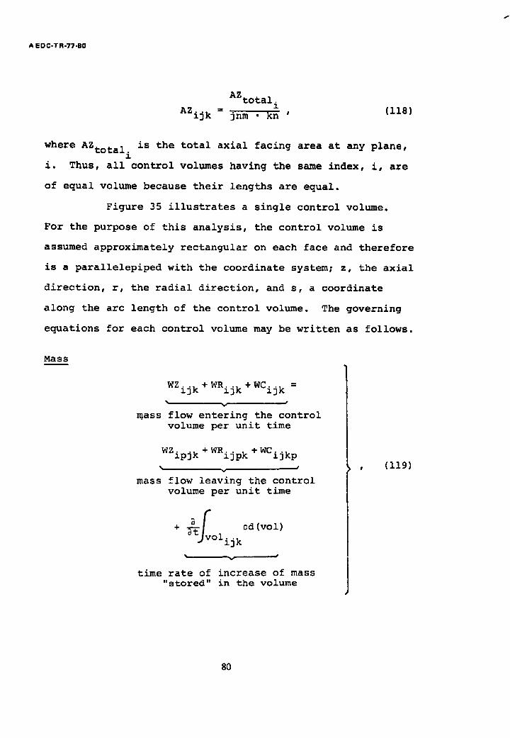
A EDC-T R-77-80
AZtotal. = I (118) AZijk jnm • kn '
where AZtotal. is the total axial facing area at any plane, 1
i. Thus, all control volumes having the same index, i, are
of equal volume because their lengths are equal.
Figure 35 illustrates a single control volume.
For the purpose of this analysis, the control volume is
assumed approximately rectangular on each face and therefore
is a parallelepiped with the coordinate system; z, the axial
direction, r, the radial direction, and s, a coordinate
along the arc length of the control volume. The governing
equations for each control volume may be written as follows.
Mass
WZij k + WRij k + WCij k =
• i
mass flow entering the control v o l u m e p e r u n i t t i m e
WZipjk + WRijpk + WCijkp
v
mass flow leaving the control v o l u m e p e r u n i t t i m e
+ ~-~f cd(vol)
°lij k
Y
time rate of increase of mass " s t o r e d " i n t h e v o l u m e
(119)
80
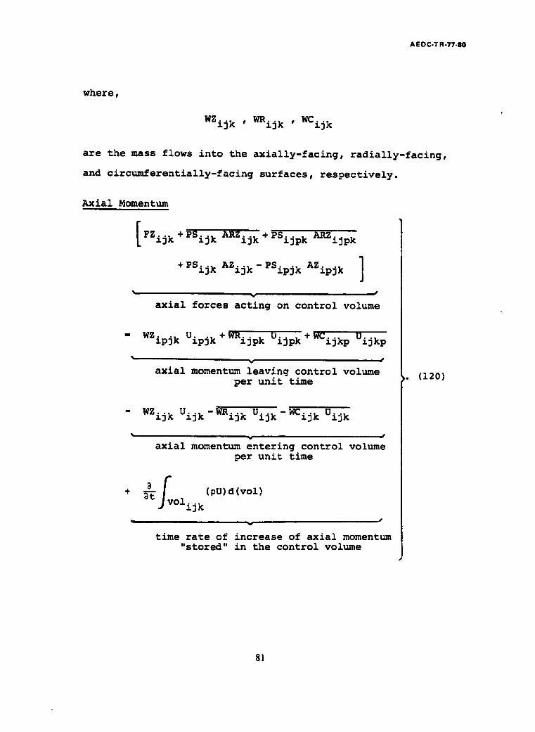
AEDC-T R-77-80
where,
WZijk ' WRijk ' igk
are the mass flows into the axially-facing, radially-facing,
and circumferentially-facing surfaces, respectively.
Axial Momentum
FZij k + ~ + P S i j p k ARZijpk
+ PSij k AZij k -PSipjk AZipjk ]
v
axial forces acting on control volume
WZipjk Uipjk + WRijpk Uijpk + WCijkp Uijkp
v J
axial momentum leaving control volume per unit time
+
WZijk Uijk-WRij k Uij k-WCij k Uij k
t
axial momentum entering control volume per unit time
v (pU) d(vol) t olij k
'v
t i m e r a t e o f i n c r e a s e o f a x i a l moment~ 'n "stored" in the control volume
, . (120)
8!
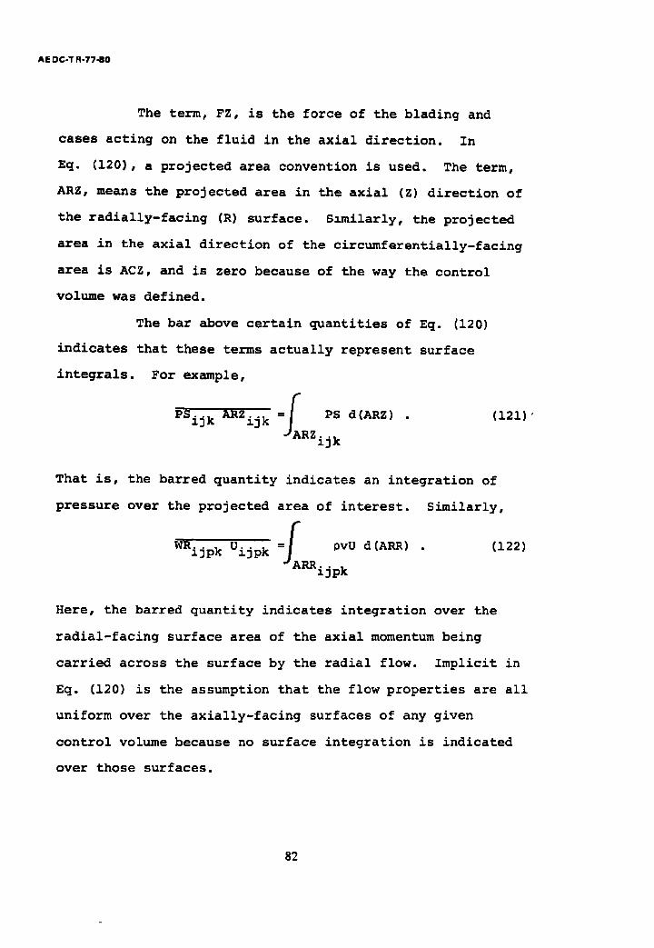
AE DC-T R-77-80
The term, FZ, is the force of the blading and
cases acting on the fluid in the axial direction. In
Eq. (120), a projected area convention is used. The term,
ARZ, means the projected area in the axial (Z) direction of
the radially-facing (R) surface. S~milarly, the projected
area in the axial direction of the circumferentially-facing
area is ACZ, and is zero because of the way the control
volume was defined.
The bar above certain quantities of Eq. (120)
indicates that these terms actually represent surface
integrals. For example,
=~A PS d (ARZ) PSij k ARZij k
RZij k
(121)"
That is, the barred quantity indicates an integration of
pressure over the projected area of interest. l "
WRijpk Uijpk =I pvU d(ARR) .
~ARRijpk
Similarly,
(122)
Here, the barred quantity indicates integration over the
radial-facing surface area of the axial momentum being
carried across the surface by the radial flow. Implicit in
Eq. (120) is the assumption that the flow properties are all
uniform over the axially-facing surfaces of any given
control volume because no surface integration is indicated
over those surfaces.
82
AE D C-T R-77-80
Radial Momentum
[FRijk + PSij k ACRij k
+PSij k ARRij k
+ PSijkp ACRijkp
I -PSijpk ARRijpk ]
% ,%. •
radial forces acting on control volume
WZipjk Vipjk +WRijpk Vijpk +WCijkp Wijkp
• ~.. I
radial momentum leaving control volume
- WZij k vij k÷WRij k Vijk+WCij k Wijk
• v
radial momentum entering control volume
+ ~--~ (0v) d (vol)
Jvol...
time rate of increase of radial momentum "stored" in the control volume
. (123)
The force, FR, includes centrifugal forces and viscous
forces acting radially on the fluid in the control volume.
83
AE DC-TR-77-80
Circumferential Momentum
+
FCij k + ~ - P S i j k p ACCijkp
v
circumferential forces acting on c o n t r o l v o l u m e
WZipjk Wipjk +WRijpk Wijpk +WCijkp Wijkp
circumferential momentum leaving control volume per unit time
WZijk wij k-WRij k wij k-WCij k wij k
v
circumferential momentum entering control volume per unit time
f (ow)d(vol)
v°lij k
v
time rate of increase of circumferential momentum "stored" in the control volume
• (124)
The force, FC, includes Coriolis and viscous forces acting
on the fluid in the control volume.
84
A E D C -T R -7"/-80
~_n e.__rr g_.,y..
w
HZij k + HRij k +
v
enthalpy entering the control volume per unit time
+ WS + Q
v
shaft work done and heat added to fluid in control volume per
unit time
HZipjk + HRijpk + HCijkp
enthalpy leaving the control volume per unit time
(125)
+ 0f [ u2.v2..2] p e + 2 d(vol)
v°lij k
time rate of increase of energy "stored" in the control volume
In Eq. (125), the barred quantities represent integrations
over surfaces similar to those of the momentum equations.
For example,
HRijk = fAR [Cp TS +
U 2 + v 2 + w 2 pv d (AR) . (126)
8S
AE DC-TR-77-80
II. SIMPLIFICATIONS
In principle, the governing equations, Eqs. (119),
(120), (123), (124), and (125), could be solved directly if
all terms entering the equations could be evaluated. There
are five differential equations for each control volume;
therefore, for the example of Fig. 34, simultaneous solution
of 360 differential equations would be required. This, in
itself is not prohibitive, but, as finer divisions of the
compressor, or, as larger compressors are considered, the
computer storage and time requirements make the analysis
inconvenient to use. Also, direct solution of the radial
and circumferential momentum equations requires knowledge of
equivalent radial and circumferential body forces not
readily determinable. Further, numerical stability becomes
more and more of a problem as the level of complexity and
number of equations are increased.
The aim of this analysis is to compute the
influence of distorted flows on compressor stability. This
goal can be achieved with simplifications to the governing
equations which circumvent, at least to an extent, the
problems listed above and produce a practical model for dis-
tortion analysis. The simplifications are as follows.
Radial and Circumferential Flows
Each control volume of the compressor is assumed
to be representable as a compressor element which is in
radial and circumferential equilibrium with adjacent control
86
AE DC-T R-77-80
volumes when the compressor is running with uniform flow at
its entry plane and uniform throttling at the exit. This
means radial and circumferential crossflows are zero with no
distortion present. Further, it is assumed that with dis-
tortion present, the radial and circumferential flow
velocities are no greater than an order of magnitude less
than the axial velocity.
The circumferential and radial crossflows into the
control volume were computed using empirical relationships
in place of the circumferential and radial momentum
equations. Algebraic expressions, relating the crossflows
to the static pressure differences between volumes, were
used. This substitution reduced the number of differential
equations requiring solution from five times to three times
the number of control volumes.
Circumferential flows. Figure 36 illustrates a
pair of control volumes circumferentially adjacent but with
different static pressures. Looking down the blades in a
spanwise direction, the flow path for the circumferential
flow is through the blade row gaps. The blade row gaps, in
effect, form a series of orifice-like restrictions to the
circumferential flow. The circumferential flow is there-
fore computed by assuming that the static pressure in the
high pressure region, PShigh, is a "reservoir" pressure
driving flow to a lower pressure, PSIo w, across a series of
87
AE DC-TR-77-80
orifices. The sequence of equations comprising the approxi-
mating algorithm is as follows.
Ec I J PShi~h 7
I m I •
Mgap PSIo w (127)
Vgap = Mgap alow pressure ' (128) region
WCgap = Plow pressure Vgap Agap region effective
(129)
The approximations of using low pressure region acoustic
velocity and density are justified because the actual
differences between adjacent control volumes are not large.
The effective gap area is given by
A = CXFC A , (130) gap gap effective physical
where CXFC is the circumferential crossflow coefficient.
For most cases, a nominal value of CXFC = 0.6 was used. The
best way to determine the coefficient value would be to
empirically calibrate it using compressor test data to pro-
vide observed crossflow values with circumferential
distortion applied to the compressor. The physical gap area
used included the space between the rotor and the stator
internal to each control volume plus the gap between the
trailing edge of the stator upstream of the control volume
and the rotor of the control volume. For the first stage,
88
AE DC-TR-77-80
the gap area was doubled to provide an accounting for the
additional circumferential flow adjustment which occurs
upstream of the compressor first rotor. Experimental data
is given in [54] which indicates the extent of the cir-
cumferential flow redistribution occurring at the compressor
entry. The process is described in detail in [38]. The
impact of crossflow magnitude on the solution is indicated
in Chapter V.
The circumferential velocity component across the
face of a control volume was computed as
V +V gaPi~ k gaPijkp (131)
Wijk = 2
The averaging is performed because the "gap" values apply
at the circumferential boundaries of the control volume.
Radial flows. Figure 37 shows a pair of radially
adjacent control volumes with different static pressure.
Viewed looking axially into the compressor, the blades form
channels in which radial flow may occur. In the actual
compressor, strong secondary flow fields caused by rotation
and viscous effects exist [55]. A considerable amount of
mass is carried back and forth across the control volume
radial boundary on a scale usually smaller than, or on the
order of, the control volume size. For the purposes of this
analysis, it is the net flow exchange, caused by distortion,
89
A E D C-T R -77 -80
which is desired. An approximate, empirical form of the
radial momentum equation is used.
WRnet = CXFRVPlow [ PShigh-PSlow] +FR • (132)
The form of the equation is a simplification of the full
radial momentum equation produced by neglecting the time-
dependent term and flux terms across all but the radial-
facing control volume boundaries. The force term, FR, is
representative of the sum of viscous and centrifugal forces,
2 FR=Fviscou s +~ vol ~ r . (133)
Because WRne t is the radial crossflow caused by distortion,
the force, FR, is adjusted so as to cause WRne t to be zero
with the compressor running with no distortion. This is, in
a sense, equivalent to imposing the radial equilibrium
condition,
2 ~P p c, r ar = ' (134)
often used in three-dimensional analysis of compressor
flows [20]. (In this application, however, FR conceptually
includes viscous forces as well as centrifugal forces.) If
the stage characteristics of each radially adjacent control
volume were the same, with no distortion present, FR would
be zero. If radial variation of stage characteristics is
90

A E D C-T S -77-80
considered (treated later in this chapter), FR is set to
cause WRne t to be zero with no distortion present.
The term, CXFR, is the radial crossflow coef-
ficient, and was determined by subjecting the model to
radial inlet distortion and adjusting the coefficient to
permit the stage exit radial static pressure gradient to
vary as much as 2% from the undistorted value. This pro-
cedure was adopted because experimental data on radial
distortion indicate that although the induced static
pressure gradients relax as the flow progresses through the
compressor, a slight gradient does remain [56]. The upper
limit of CXFR was set by model numerical stability con-
siderations. A value of CXFR = 0.01 was used for most cases
computed in this study. For modeling a specific compressor,
the value of CXFR would best be determined through tests of
a compressor with radial distortion imposed and, adjustment
of the coefficient made to match the observed change in
stage exit flow distributions caused by the radial
distortion.
The radial velocity across the boundary is
computed from,
WRne t VR = (135)
Plow Achannel
9!
AE D C-T R-77-80
The radial velocity component across the face of the control
volume was computed as
VRij k + VRijpk Vijk = 2 " (136)
III. SPECIAL CONSIDERATIONS FOR
DISTORTION EFFECTS
Radial Distortion
Figure 38 illustrates the key physical processes
occurring when a radially distorted flow approaches a rotor
blade. On the left of Fig. 38, with uniform flow, con-
sidering the "design A" case, the tip and hub angles of
attack and stage characteristic operating points are stable,
near design conditions. On the right side of Fig. 38, a hub
radial distortion (low velocity or total pressure in the hub
region) case is shown. For case "A," the tip section
operates at a lower angle of attack and higher flow coef-
ficient while the hub becomes highly loaded, and, in case
"A," is even stalled.
In the "design "B" case, the tip section in uni-
form flow is highly loaded while the hub section is only
lightly loaded. Introduction of the radial distortion
pattern for the "B" case causes the stage to operate at a
better condition than was experienced with uniform flow.
This illustrates that the way a compressor responds to
radial distortion must depend on the spanwise work
92
AEDC-TR -77-80
distribution. Therefore, the one-dimensional stage
characteristic used up to this point will not permit compu-
tation of radial distortion effects. As noted in Fig. 38,
the distortion induced shift in radial work distribution, as
well as the distorted flow pattern itself, induces radial
crossflows.
The three effects which must be considered for
radial distortion analysis are then as follows.
Radial variation of compressor entry flow
properties. These are automatically treated by the model
because of the division of the compressor into control
volumes radially as well as circumferentially.
Radial variation of work and force distribution.
Stage characteristics may be specified for each radial
location in the same manner as a single, average stage
characteristic was specified for the one-dimensional
analysis. For the example of Fig. 34, each stage would have
a hub, a midspan, and a tip set of stage characteristics.
For the XC-I compressor used in example calcu-
lations in Chapter V, the compressor was divided radially
into five annuli (jn = 6). Stage characteristics for each
annulus were not available, but radial distributions of
total pressure and total temperature at each stage discharge
were given in [43] for one operating point at the corrected
speed setting analyzed. These profile data were used to
compute a correction to stage pressure ratio and stage
93
A E D C-T R -77-80
temperature ratio as a function of radius for each stage;
thus, in effect, producing radially variant stage charac-
teristics. A total temperature ratio correction factor,
CF T(r) = TR(r) TR ' (137)
avg
and a total pressure ratio correction factor,
CF P(r) = PR(r) (138) PRavg '
were determined for each stage from the profile data of
[43].
become The stage characteristics as functions of radius then
-1 ~t _1 U 2
~T(r) =~Tvg CF T+~'w-~h|[CFT-1]
and
~P (r) = ~P 7 avg cFP
(139)
(140)
Inherent in this correction is the assumption that the
pressure ratio and temperature ratio profiles, normalized by
their averages, do not vary greatly over the range of flow
coefficient of interest. Examination of data from other
compressors where profile data were available over a wider
range of operating conditions than used in this study showed
the profiles' shapes to be consistent (within ±5%, and
usually better) up to the point of stall.
94
AEDC-TR-77-80
Radial crossflows. Radial crossflows are computed
as described previously. A stage coefficient correction for
the distortion-induced radial flow velocity across the
control volume face is made by computing ~ as
U2 - v 2 ¢ U2 . (141)
wh
Circumferential distortion steady flow effects.
Figure 39a shows a compressor subjected to a simple circum-
ferential distortion pattern. Half of the face of the
compressor is in a lower than average total pressure region
and half is above. The example distortion waveform is a
simple sine wave. Upstream of the compressor face a length
of one compressor diameter or more, the static pressure
variatlon across the entry duct caused by the presence of
the compressor in the distorted flow field will be nearly
zero. The total pressure distortion at that location is
then principally an axial velocity distortion. Depending on
design characteristics and operating conditions of the
compressor, a portion of the high velocity region will be
diffused, creating a circumferential static pressure
gradient at the compressor face. This results in the
generation of a swirl velocity (Fig. 39a) carrying mass from
the high to the low pressure regions of the compressor face.
(This phenomenon is described in more detail in [27, 38,
54].) Figure 39a shows the influence of the variation in
95

A EDC-TR-77-80
axial and swirl velocities at four circumferential locations.
At 8 = 0, there is no swirl velocity and axial velocity is
high; therefore, ~ is low and the stage is operating at a
lightly loaded condition. At 8 = 90 °, the axial velocity is
still fairly high, and the swirl component exists, and is in
the direction of rotor rotation. The swirl component
combines with wheel speed to reduce the angle of attack at
this point. At 8 = 180 ° , the axial velocity is at a
minimum, thus causing a high angle of attack and high, even
stalled, stage loading. At 8 = 270 °, the axial velocity is
increased once more, but the swirl velocity component is
counter to rotor speed, thereby causing a higher angle of
attack and stage loading.
To a lesser extent, the same flow situation exists
at each stage entry. The effects on the stage character-
istic operating points are accounted for by computation of
the flow coefficient as
U = +V " (142)
Uwh sw
The swirl velocity, Vsw , is simply the circumferential
velocity component, w, at that particular location.
Unsteady effects. Figure 39b illustrates unsteady
airfoil effects for the same circumferential distortion
pattern. As indicated in Fig. 39b, the axial and swirl
velocities caused the flow coefficient to decrease, even to
96
AE DC-TR-77-80
below the steady-state stage stall value. The distortion
pattern is stationary. The rotor blades pass through the
spatially variant stationary pattern with each rotation,
and, from their point of reference, the flow is cyclically
unsteady. For a sinusoidal pattern, the frequency felt by a
rotor blade is
N f = 2--~ = ~ , (143)
where N is the mechanical rotor speed in rpm.
If the distortion pattern contained two cycles of
a sine wave instead of one (i.e., two low pressure regions),
the frequency would double. The reduced frequency for the
blade is
k = 2~fC _ NC (144) Vre I 60 Vre I
As discussed in Chapter II, the blade forces cannot instan-
taneously respond to rapid changes in angle of attack.
Therefore, as a blade passes through the low pressure region
(region of low %, Fig. 39b), the blade forces, thus ~, do
not follow the # variation in a steady-state manner. Near
the stall point, if the variation is sufficiently rapid, the
lag is such that ¢ may proceed into the stalled region, and
quickly retreat, without blade stall actually occurring
[35]. The effect is more pronounced as reduced frequency
increases.
97
AE DC-T R-77-80
The unsteady cascade aerodynamics arising Item
circumferentlal distortion are approximated in the model
following the treatment described in Chapter If, with an
empirical correction added for the stalled blade region of
operation. In Figs. Ii and 14, the unsteady lift magnitude
is given as a function of reduced frequency. As was shown
in Chapter II, Eq. (58), the dynamic response of ~ is the
same as the dynamic response of C£. Therefore, the ratio of
maximum dynamic ~ to the quasi-steady-state value is the
same as the corresponding lift coefficient ratio. Or,
I Imax Ic Imax Iss Ic Iss
= DLR . (145)
(DLR means dynamic lift ratio.)
Referring to the upper left-hand corner of
Fig. 39b, as a rotor blade begins at location k = I, the
value of ~ is ~i" As it progresses to the low pressure
area, k = 4, ~ = ~4" The value of #4 calculated on a
steady flow basis in region k = 4 is ~4 , but, is incorrect ss
because of dynamic effects. Let the actual value be ~4dy n.
A correction may be constructed as follows.
- 41 I ¢ I ma x ~4d~ n - = DLR (146)
ss ss
98
A E D C-T R -77-80
Therefore,
4dy n ' + (i - DLR) ~i " = DLR ~4s s (147)
Thus, the actual ~4 value depends not only on the steady-
state value computed at the k = 4 location, but also on the
blade's history as it passed from location k = I.
This dynamic lag algorithm can be more generally
written so as to be applied successively from one sector to
the proceeding sector in the direction of rotor rotation.
Or,
~ijk = DLR ~ijks s + (i - DLR) ~ijkm " (148)
Thus, a lag is introduced into the stage characteristics.
The value of DLR used was computed from
i
DLR = -~/ 1
V 1 + (ak) , (149)
as shown in Fig. 14. The reduced frequency, k, depended on
the shape of the circumferential distortion pattern. The
value of £ used followed the Goethert-Reddy analysis, but
could readily be varied based on measured response of a
compressor to circumferential distortion of varying pattern
shape to account for additional viscous effects. This
part of the unsteady correction predominates in the blade
unstalled region of operation.
99
AE DC-TR-77-80
Goethert and Reddy point out in [32] that blade
dynamic response should be expected to be more sluggish
because of boundary layer effects not included in their
inviscid analysis. This will be particularly true when the
blade is operating in its stalled region. As already
pointed out, the blade may transiently operate at angles of
attack greater than the steady-state stall angle of attack
without actually stalling. Experimental results on the
degree to which this phenomenon may be present for isolated
airfoils were compiled by Melick [36] and are indicated in
Fig. 39c. The dynamic stall lift coefficient increment is
correlated to the nondimensional time derivative of angle of
attack for several different types of isolated airfoils.
This effect was incorporated in the model by
computing the derivative of angle of attack from the change
in flow coefficient as a blade passed through the distortion
pattern using Eq. (34) to relate flow coefficient to angle
of attack. A stall lift coefficient increment was then
calculated using the empirical relationship of Fig. 39c.
The resulting lift coefficient increment was then used to
compute an equivalent increment in stage pressure and
temperature coefficients using Eq. (39), neglecting the
influence of the blade drag coefficient. With this infor-
mation, the stage characteristic curve was translated
upward, at the unstalled stage characteristic slope existing
near the stage characteristic peak, in a manner analogous to
the CE - ~ curve translation of Fig. 39c. This translation,
100
AEDC-TR -77-80
when combined with the dynamic lag effects of Eq. (149)
yields the dynamic stage characteristic behavior in the
stalled stage region depicted in Fig. 39b.
The Goethert-Reddy analysis [32] and Fig. ii
indicated less dynamic effects with a cascade of airfoils
than are experienced with a single, isolated airfoil. It
might well be anticipated that the stall region behavior of
the cascade would be less than the isolated airfoil case as
well. For that reason, the "stall overshoot" constant, m,
Fig. 39c, was chosen at four different values, and influence
on the solution determined parametrically. A value of m
between one and ten was found to be reasonable. Details of
the parametric investigation are discussed in Chapter V.
IV. METHOD OF SOLUTION
In this section, the approximation to the time
derivative of the volume integrals in the governing
equations is described. The resulting model equations,
including effects of the simplifications already described,
are written and the solution procedure described.
Volume Integral Time-Derivative Approximation
In each of the governing equations, Eqs. (119),
(120), and (125), a partial time derivative of a volume
integral exists. The general form is
101
AEDC-TR-7740
Y = ~t l~" y (z,r,s,t) d(vol)
#v ol
= f ~Y (z,r,s t) d(vol) ~t ' " Jv ol
(150)
It is desired to approximate Y in terms of a control volume
surface value of y. By the mean value theorem, there exists
some point (z,r,s) interior to the control volume, such that
fro ~ (z'r's't) d(vol) = (vol} ~ (z,r,s,t) .
1
(151)
~Yo Let -~£- be a value of the integrand on either the forward or
aft control volume face normal to the z-axis. The time
derivative at the mean value point is then related to the
surface time derivative by expanding around the surface
point,
where
~Y (z,r s t)=°Y [ z O So t ] ~t ' ' ~t 'ro' '
Z O +a~Z,ro,So,t ] ] Az
[ "o,ro, o
o < a, b, c < 1
, (152)
102
AE DC-TR-77-80
Also,
and
AZ = Z - ~ O
Ar= r - r o
AS = S O -
(153)
The approximation,
~Yo ¥ = (vol) ~- , (154)
is chosen for use in the model. Multiplying Eq. (152) by
the volume, and rearranging the order of differentiation
yields an estimate for the truncation error.
E -" (vol) ~-~ AZ + ~r
The spatial derivatives are finite; therefore, as
Az , Ar , As ~ 0 ,
(155)
the error, c, vanishes, thus the approximation is consistent
of order one.
Numerical stability was investigated by running
with different time step sizes as in the one-dimensional
analysis. A time step size of approximately one-half the
value indicated by the Courant-Friedrichs-Lewy criterion
was used.
103
AE DC-TA-77-80
The actual approximations made were,
Mass
p d(vol) = vol ~ Pipjk '
d volijk
(156)
Axial Momentum
~-~ (p U) d(vol) = vol (p U)
v°lij k
ijk ' (157)
Energy
~fv Pie+
°lij k
U 2 + v 2 + w 2 2 J d (vol)
= vol ~ p e+ 2 ipjk
(158)
Model Equations
Using the approximations and simplifications pre-
viously described yields the equations comprising the
distortion model.
Governing Equations
Mass, axial momentum, and energy were used. The
assumption of small v and w permits ignoring v and w terms
104
AEDC-TR-77-80
in some instances. Also, radial and circumferential flows
were determined by the crossflow approximations, thus
replacing the radial and circumferential momentum equations.
The resulting equations are as follows.
Mass
a ipjk 1 [ ~t - volij k WZijk + WRijk + WCijk
- WZipjk -WRijpk - WCijkp ] " (159)
Axial Momentum
8 ( P U)i~k = 1 [ ] (160) ~t ~ Fijk + IMPijk - IMPipjk "
In Eq. (160) the contribution of the pressure integrated
over the projected areas of the radially oriented surfaces
is combined with the force term, FZ, of Eq. (120) to pro-
duce F. The force, F, is obtained from stage characteristic
information, as was done in the one-dimensional case. The
impulse terms are
IMP = PS AZ + WZ U . (161)
The momentum convected across the radial and circumferential
boundaries is negligible compared to the axial impulse terms.
105
AED C-TR-77-80
Energy
xi [ ] -- 1
(vol)ii k ~ijk + QiJk + I~ijk - HZipjk • (162)
In Eq. (162),
[ u2 ] X = p e + -~- . (163)
The v 2 and w 2 terms in Eq. (125) are negligible compared to
U 2 .
The terms neglected in Eqs. (160) and (162) are
second-order terms determined by nondimensionalization and
order of magnitude analysis of the equations• The terms
were ignored because their influence on the solution was
small. Also, inclusion of terms caused the numerical solu-
tions to be generally less stable and to oscillate with
small amplitude when a steady-state condition was reached.
Solution Procedure
The solution procedure used on the digital
computer paralleled the approach used for the one-
dimensional model outlined in Fig. 16. Initial values of
the dependent variables, D, P U, and X, were specified for
every control volume location, ijk, to start the solution.
For simplicity, the solution was always started from a
steady, uniform flow condition, thus easing the chore of
computing initial conditions.
106
AEDC-TR-77-80
Forward boundary conditions. Forward boundary
conditions were total pressure and total temperature,
Pl,j,k and Tl,j,k, specified at each control voiume face.
Entry plane conditions were then computed using the same
relationships as indicated in Fig. 16, but for every control
volume face instead of just one. Thus, the subscript, i, in
Fig. 16, entry plane conditions, is replaced with subscript,
l,j,k.
Interior plane values. The same relationships
indicated in Fig. 16 are used again. Once more, the
subscript, i, must be replaced with i,j,k, and the quanti-
ties computed at each control volume face.
Crossflow values. Crossflows among the control
volumes are computed using Eqs. (127) through (136) for each
control volume. For all calculations made in this study,
crossflow across the compressor walls was zero.
Exit plane conditions. Only unchoked flow at the
exit was used for this study; thus, a uniform static
pressure was specified at every control volume aft face at
the compressor exit plane. Exit plane calculations follow-
ing the unchoked portion of the one-dimensional procedure
(Fig. 16, exit plane conditions) were therefore used with
the index, in, replaced by in,j,k, and computations made for
all control volumes.
107
A E D C-T R-77 -80
Force and work computations. The same procedure
used in the one-dimensional procedure was used again, but
individually at each control volume. Local values of flow
coefficient were computed and adjusted for distortion
effects according to Eqs. (141) and (142). Further cor-
rections to stage characteristics for radial variations and
for unsteady effects were also made.
Time-derivative computations. The derivatives of
the dependent variables, D, p U, and X, are computed from
Eqs. (159), (160), and (162) for every control volume. The
values are then integrated to provide values of the vari-
ables at the next time step. The sequence is then repeated,
with the boundary conditions changing in accordance with the
specified problem under investigation and the computations
continued until the desired solution is obtained.
Additional numerical stability considerations. To
prevent numerical instabilities in the model solution caused
by error buildup in the crossflow calculations when the
driving pressure differences from control volume to control
volume are very small, the pressure differences are tested
to assure a significant pressure gradient exists. If a
significant difference exists, crossflow is calculated; if
not, crossflow is set to zero.
108

AE D C-TR-77-80
CHAPTER V
EXAMPLE PROBLEMS WITH COMPARISON TO EXPERIMENTS,
DISTORTION MODEL
One steady-state combined radial and circumfer-
ential distortion case for the XC-I compressor is given.
Detailed experimental data were available for this case and
comparisons between model computations and experimental
measurements are presented. An example of time-variant
distortion for the XC-I compressor is given. Pure radial
and pure circumferential distortion effects are computed.
A pure circumferential temperature distortion case is also
presented. Specific experimental data were not available
for the time-variant distortion, pure radial and pure
circumferential distortion patterns for the XC-I compressor.
Data from other compressor tests were used, therefore, to
check the model results for proper trend and order of
magnitude.
In all cases discussed in this chapter, the
nominal compressor entry conditions were one atmosphere
pressure and 518.7°R temperature.
I. COMBINED DISTORTION PATTERN, XC-1 COMPRESSOR
Figure 40 shows a contour map of the combined
circumferential and radial total pressure distortion pattern
to which the XC-I compressor was subjected. The pattern was
109
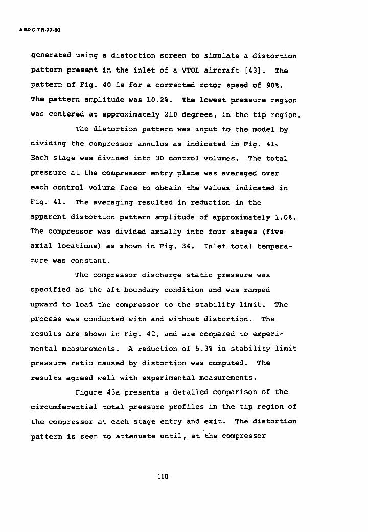
AED C-TR-77-80
generated using a distortion screen to simulate a distortion
pattern present in the inlet of a VTOL aircraft [43]. The
pattern of Fig. 40 is for a corrected rotor speed of 90%.
The pattern amplitude was 10.2%. The lowest pressure region
was centered at approximately 210 degrees, in the tip region.
The distortion pattern was input to the model by
dividing the compressor annulus as indicated in Fig. 414
Each stage was divided into 30 control volumes. The total
pressure at the compressor entry plane was averaged over
each control volume face to obtain the values indicated in
Fig. 41. The averaging resulted in reduction in the
apparent distortion pattern amplitude of approximately 1.0%.
The compressor was divided axially into four stages (five
axial locations) as shown in Fig. 34. Inlet total tempera-
ture was constant.
The compressor discharge static pressure was
specified as the aft boundary condition and was ramped
upward to load the compressor to the stability limit. The
process was conducted with and without distortion. The
results are shown in Fig. 42, and are compared to experi-
mental measurements. A reduction of 5.3% in stability limit
pressure ratio caused by distortion was computed. The
results agreed well with experimental measurements.
Figure 43a presents a detailed comparison of the
circumferential total pressure profiles in the tip region of
the compressor at each stage entry and exit. The distortion
pattern is seen to attenuate until, at the compressor
110
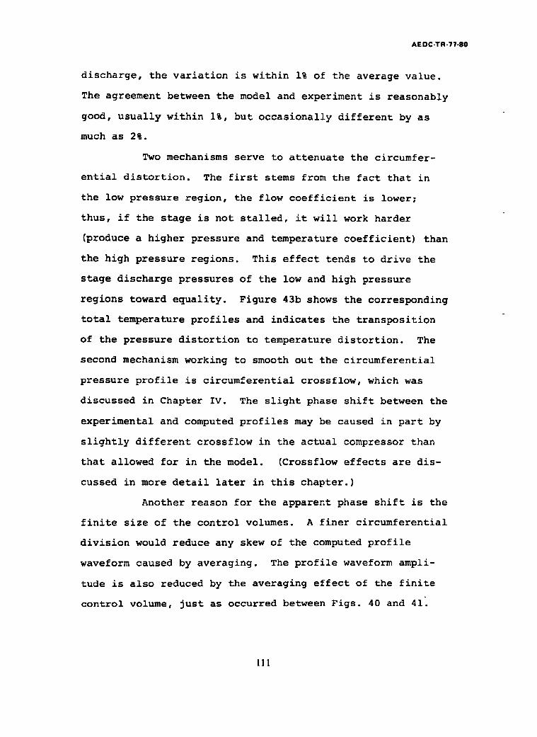
AEDC-TR-77-80
discharge, the variation is within 1% of the average value.
The agreement between the model and experiment is reasonably
good, usually within i%, but occasionally different by as
much as 2%.
Two mechanisms serve to attenuate the circumfer-
ential distortion. The first stems from the fact that in
the low pressure region, the flow coefficient is lower;
thus, if the stage is not stalled, it will work harder
(produce a higher pressure and temperature coefficient) than
the high pressure regions. This effect tends to drive the
stage discharge pressures of the low and high pressure
regions toward equality. Figure 43b shows the corresponding
total temperature profiles and indicates the transposition
of the pressure distortion to temperature distortion. The
second mechanism working to smooth out the circumferential
pressure profile is circumferential crossflow, which was
discussed in Chapter IV. The slight phase shift between the
experimental and computed profiles may be caused in part by
slightly different crossflow in the actual compressor than
that allowed for in the model. (Crossflow effects are dis-
cussed in more detail later in this chapter.)
Another reason for the apparent phase shift is the
finite size of the control volumes. A finer circumferential
division would reduce any skew of the computed profile
waveform caused by averaging. The profile waveform ampli-
tude is also reduced by the averaging effect of the finite
control volume, just as occurred between Figs. 40 and 41
111

AE DC-TR-77-80
Thus, the model profile amplitudes should be expected to be
1% or so less than the experimentally observed profiles.
Figure 44 shows the attenuation of the distortion
pattern through the compressor for the tip (Fig. 44a),
mid-span (Fig. 44b), and hub (Fig. 44c) regions. Agreement
between the computed and experimental results is generally
within 1% when allowance is made for the averaging effects
of the finite control volumes of the model. Pressure dis-
tortion reduction and tomperature distortion production are
similar for the tip and mid-span regions. In the hub
region, however, both the computed and experimental measure-
ments indicate amplification of the distortion across the
first stage. This occurs because of the shallower stage
characteristics which exist in the hub region. The agree-
ment is not as good in the hub region as in the tip and
mid-span regions, indicating some inaccuracy in the
estimation of the hub region stage characteristics.
Figure 45 presents a comparison of radial total
pressure and temperature profiles in the region of maximum
radial distortzon (at 210 degrees). Figure 45a shows agree-
ment within 1 to 2% except in the hub region at the second
stage entry. Once more, this indicates some inaccuracy in
the hub region stage characteristic. Figure 45b shows the
total temperature radial profiles. Agreement within 1% was
generally achieved.
Figure 46 presents similar profiles for the
compressor operating without distortion. Agreement between
!12
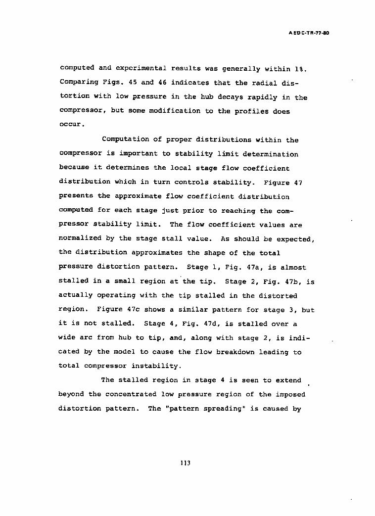
A ED C-TR-77-80
computed and experimental results was generally within 1%.
Comparing Figs. 45 and 46 indicates that the radial dis-
tortion with low pressure in the hub decays rapidly in the
compressor, but some modification to the profiles does
occur.
Computation of proper distributions within the
compressor is important to stability limit determination
because it determines the local stage flow coefficient
distribution which in turn controls stability. Figure 47
presents the approximate flow coefficient distribution
computed for each stage just prior to reaching the com-
pressor stability limit. The flow coefficient values are
normalized by the stage stall value. As should be expected,
the distribution approximates the shape of the total
pressure distortion pattern• Stage i, Fig. 47a, is almost
stalled in a small region at the tip. Stage 2, Fig. 47b, is
actually operating with the tip stalled in the distorted
region. Figure 47c shows a similar pattern for stage 3, but
it is not stalled. Stage 4, Fig. 47d, is stalled over a
wide arc from hub to tip, and, along with stage 2, is indi-
cated by the model to cause the flow breakdown leading to
total compressor instability.
The stalled region in stage 4 is seen to extend
beyond the concentrated low pressure region of the imposed
distortion pattern. The "pattern spreading" is caused by
113
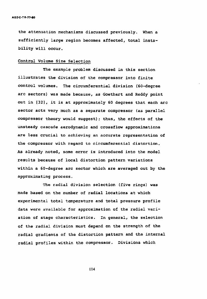
AED C-TR-77-80
the attenuation mechanisms discussed previously. When a
sufficiently large region becomes affected, total insta-
bility will occur.
Control Volume Size Selection
The example problem discussed in this section
illustrates the division of the compressor into finite
control volumes. The circumferential division (60-degree
arc sectors) was made because, as Goethert and Reddy point
out in [32], it is at approximately 60 degrees that each arc
sector acts very much as a separate compressor (as parallel
compressor theory would suggest); thus, the effects of the
unsteady cascade aerodynamic and crossflow approximations
are less crucial to achieving an accurate representation of
the compressor with regard to circumferential distortion.
As already noted, some error is introduced into the model
results because of local distortion pattern variations
within a 60-degree arc sector which are averaged out by the
approximating process.
The radial division selection (five rings) was
made based on the number of radial locations at which
experimental total temperature and total pressure profile
data were available for approximation of the radial vari-
ation of stage characteristics. In general, the selection
of the radial division must depend on the strength of the
radial gradients of the distortion pattern and the internal
radial profiles within the compressor. Divisions which
I14
AE DC-TR-77-80
hold averaging error to within 1 or 2% should be quite
sufficient. Also, the radial crossflow representation in
the model is relatively crude. Therefore, it should not be
expected that finer and finer radial division of the com-
pressor would yield greater and greater accuracy of the
computed results. Additionally, the stage characteristic
data are based on one-dimensional (or, at best, averaged
over a radial distance) data, thus, a very fine division
radially would not be consistent with the resolution of the
input empirical information.
II. TIME-VARIANT DISTORTION
Figure 48 illustrates time-variant distortion.
The total pressure at the engine entry plane fluctuates with
time and also varies spatially across the compressor face.
The fluctuations are caused by unsteady flow processes in
the inlet, such as unsteady shock wave-boundary layer
separation [6, 13, 15]. The unsteady, nonuniform flow
causes distortlon patterns at the engine entry which vary
with time, as illustrated in Fig. 48. The spatially
averaged pressure also oscillates.
The XC-I compressor model was subjected to tlme-
varlant distortion by superimposing a time-dependent
waveform on the distortion pattern of Fig. 40. Figure 49
shows the frequency spectrum of the superimposed fluctu-
ations. The spectrum is representative of those measured
experimentally in aircraft inlets [15]. The waveform was
115
A E DC-TR-77-80
applied in two parts. One part was phase shifted over the
compressor face so as to alternately stretch and shrink the
steady-state distortion pattern. The other part was added
uniformly to produce timewise fluctuation in the spatial
average. (Details of time-variant distortion pattern
analysis and synthesis are discussed in [42].)
Two cases were computed for the XC-I compressor
with time-variant distortion. One was for an overall root-
mean-square (rms) amplitude of 2% and the other was for 4%.
With these inlet flow fields present, the compressor exit
pressure was ramped upward until instability occured.
Figure 50a shows the loss in stability limit pressure ratio
correlated with the rms amplitude. A reduction results, as
should be expected, and is of similar magnitude as the
experimental results of [7] for a different compressor.
The model computed results were also correlated to
the amplitude of the instantaneous distortion pattern
existing just prior to compressor instability, as shown in
Fig. 50b. All pattern shapes were similar, thereby per-
mitring use of the simple distortion pattern magnitude
descriptor. The results generalize well with steady-state
distortion results, thus providing a degree of analytical
conformation to the quasi-steady-state distortion approach
currently used in experimental stability analysis. (See
Chapter I and [7] for further details on that approach.)
The results shown in Fig. 50 should not be sur-
prising because the XC-1 compressor is very small (about
116
A E D C-T R -77-80
17 inches in diameter and 8 inches long) and has high rotor
speed (about 16,230 rpm at 90% speed). Therefore, fluctu-
ations in the frequency range considered are sufficiently
low to permit the instantaneous distortion pattern to dwell
at the entry, and penetrate through the compressor in a
quasi-steady manner. For example, in this case, approxi-
mately 0.0037 second is required for one rotor revolution,
and 0.0017 second is required to convect a particle through
the compressor (average axial velocity of 400 ft/sec). The
period of the highest frequency component in the spectrum is
0.0038 second. Thus, the distortion effects will be much
like steady-state distortion.
If larger amplitude timewise fluctuations are con-
sidered, particularly if the compressor is combined with
upstream ducting and a combustor, planar oscillation effects
similar to those discussed in Chapter III would show an
effect also.
III. PURE RADIAL AND CIRCUMFERENTIAL
DISTORTION PATTERNS
Three additional types of distortion patterns were
computed to gain some insight into the influence of pattern
severity and shape v~riations. The patterns considered are
pure radial pressure distortion, pure circumferential
pressure distortion, and pure circumferential temperature dis-
tortion. No specific experimental data for the XC-I
117
AE DC-TR-77-80
compressor were available for these cases. Comparisons to
experimental results from other compressors are made
therefore.
Radial Pressure Distortion
Figure 51a illustrates the results of loading the
XC-I compressor model to the stability limit with tip radial
distortion (low pressure in the tip region). Pattern
severities of 5, i0, and 20% were considered. Because of
the relatively high tip loading of this compressor, Fig. 46,
it appears to be more sensitive to tip radial distortion.
Figure 51b shows the results for the hub radial case and
indicates the compressor to be more tolerant. Figure 52
shows comparisons of the XC-1 model results with experi-
mental data from a J85-13 test [16]. Similar results were
obtained, except that the J85-13 was even more tolerant of
hub radial distortion than the XC-I was computed to be.
Circumferential Pressure Distortion
Figure 53 shows the effect of increasing the
severity of a 60-degree-arc circumferential distortion
pattern. Pattern magnitudes of 5, i0, 15, and 20% were
computed. Increasing loss of stability limit pressure ratio
and airflow was computed. Figure 54 shows the model
results compared to a range of experimental data from other
compressors. The model results appear reasonable.
Figure 55a depicts the variation of airflow in the
distorted region. Crossflow into the distorted region
118
AEDC-TR-77-80
rapidly increases the flow in that sector. Also shown in
Fig. 55a is the crossflow into an approximately 90-degree
distorted region computed for the XC-I compressor from
experimental measurements [43].
Two different crossflow distribution cases were
computed to check the influence of crossflow on computed
compressor behavior. In one case, the first stage cross-
flow was increased. The increase was accomplished by
increasing the first stage crossflow area. Figure 55b indi-
cates the effect of the crossflow change on compressor
stability. The increased first stage crossflow case
matched the experimental distribution better, and caused a
higher stability limit pressure ratio with distortion
present. The improved performance comes about by allowing
crossflow to relieve downstream stage loading in the dis-
torted region. The crossflow distribution more closely
matching the experimental case was used in the previously
discussed combined distortion case.
Figure 56 shows the influence on stability of
varying the angular extent of the circumferential low
pressure area while holding the distortion pattern magnitude
constant. Three different cases, 6- = 30, 60, and 180
degrees are shown. The 30-degree case has the least loss in
stability. The 60- and 180-degree cases have approximately
the same percentage loss in stability limit pressure ratio
(taken at constant corrected airflow through each stability
limit point). However, the flow and pressure ratio
119
AE DC-TR-77-80
reduction for the 180-degree case was more than that of the
60-degree case. Figure 57 shows the loss in stability limit
pressure ratio as a function of distortion pattern angular
extent. Computations were made for four different values of
dynamic lift coefficient "stall overshoot" constant, m,
Fig. 39c. Also shown in Fig. 57 are experimental data from
a J85-13 compressor subjected to distortion of varying
angular extent. The experimental results fall between the
m = 1 and m = i0 model computation results. The m = 40
results, corresponding to the center of the isolated airfoil
correlation curve, Fig. 39c, produce virtual insensitivity
to circumferential distortion up to 60 degrees, which is an
unrealistic result. A value of m between 1 and i0 is a
more realistic value. The results shown in Fig. 56 are for
m = i0.
The analysis presented in Fig. 57 indicates that
the unsteady cascade aerodynamic effects predominate in
determining the response of the compressor to circumfer-
ential distortion below approximately 60 degrees angular
extent.
Circumferential Temperature Distortion
Figure 58 shows the effect of varying the severity
of total temperature distortion on compressor stability.
Temperature distortion destabilizes the compressor in much
the same manner as does pressure distortion. The distorted
region, which is hotter than the rest of the compressor,
120
AEDC-TR-7?-80
operates at reduced airflow, thus at reduced flow coef-
ficients compared to the rest of the compressor. Therefore,
as the load on the compressor is increased, the hot region
stalls first, eventually causing the entire compressor to
become unstable.
Mechanical rotor speed was constant during the
loading. Corrected rotor speed, indicated in Fig. 58,
decreased as much as 1.1% because of the increased average
temperature over the face of the compressor.
Little influence of crossflow was found, indi-
cating that basic parallel compressor theory (with
appropriate unsteady cascade corrections) should give
reasonable predictions for temperature distortion.
Figure 59 shows a comparison of model computed
stability limit pressure ratio reduction to experimental
results from other compressors. The predicted trend is
reasonable, although more pressure ratio reduction is
computed than was experienced on the other compressors.
121
AEDC-TR-77-80
CI~PTER VI
SUMMARY OF RESULTS AND RECOMMENDATIONS
FOR FURTHER WORK
The overall objective of this work was to develop
an improved analytical method for the computation of turbine
engine compressor stability loss caused by a wide range of
different types of external flow disturbances. Another
objective was to gain understanding of the physical
processes leading up to instability as induced by external
disturbances. The understanding was provided by the
development of an analytical model and by application of the
model to example problems with comparisons to experimental
results. The objectives were accomplished in two major
steps. In the first step, a one-dimensional, time-dependent
math model was developed and applied to a variety of steady
and time-dependent planar disturbances which are destabi-
lizing to the compressor. In the second step, the concepts
of the one-dimensional model were extended to three
dimensions to allow the development of a time-dependent
model for computation of radial, circumferential and
combined distortion effects on stability. The distortion
model was then applied to the computation of distortion
cases with comparisons to experimental results. The results
of those two steps are summarized as follows.
122
AEDC-TR-77-80
I. ONE-DIMENSIONAL, TIME-DEPENDENT ANALYSIS
Model Description
The one-dimensional model satisfies the time-
dependent mass, momentum and energy equations. The full,
nonlinear form of the equations, not used in earlier works,
was used. The compressor is divided into control volumes on
a stage-by-stage basis. The force and shaft work applied to
the fluid is determined from empirical steady-state stage
characteristics modified for unsteady cascade airfoil
effects. The solution of the model governing equations is
obtained through finite difference approximation of the
governing differential equations. The resulting system of
equations was solved on a digital computer.
Example Problems
Steady-state stabilit~ limit. Three different
compressors were modeled. They were, an Allison XC-I lift
engine four-stage compressor, a NACA eight-stage research
compressor, and the General Electric J85-13 turbojet engine
compressor. The model was shown to be able to generally
compute the steady-state stability limit pressure ratio and
corrected airflow to within 1 to 2% of experimentally
determined values. Compressor internal steady-state flow
conditions in agreement with experimental values were also
shown to be computed by the model. The initial flow
123
AE DC-TR-77-80
breakdown process in the compressor at the stability limit
was shown to be reasonably well reproduced by the model.
D~namic stabilit~ limits (oscillatin~ inflow
loadin~)~ NACA ei~ht-sta~e compressor. The NACA eight-stage
compressor model was driven to its stability limit by planar
oscillation of the compressor inlet pressure at frequencies
from 20 to 320 Hz. The model results indicated that, as
frequency increased, the amplitude required to cause insta-
bility decreased. It also showed that the individual stages
transiently enter and retreat from their stalled regions
during the oscillations without total compressor instability
occurring. As the oscillation amplitude increased, however,
the time period during which the stage is in the stalled
region is increased, and a point is eventually reached where
total compressor instability occurs. The analysis showed
further that, for planar oscillations in the frequency range
analyzed, the influence on stability of the unsteady cascade
correction to the steady-state stage characteristics was
small.
The ability of the model to compute dynamic
stability limits was shown to depend strongly on the model's
ability to properly compute the dynamic response of the
compressor to imposed disturbances.
Oscillating inflow dynamic response, J85-13
compressor. The unstalled, dynamic response to planar entry
pressure oscillations in terms of amplitude ratio and phase
1:24
AE DC-TR-77-80
angle were computed and compared to experimental data. The
experimental data were obtained by NASA in a wind tunnel at
Math 2.5 with the engine operating behind a supersonic
inlet. The compressor entry pressure oscillations were pro-
duced by forced oscillations of the inlet bypass doors.
Data were acquired from 1 to 50 Hz. Amplitude ratios and
phase angles computed by the model agreed with experimental
values to within 10% and five degrees, respectively. An
additional set of experimental oscillating entry pressure
data obtained by NASA was compared to the inlet data and
model computations. The additional set was obtained in a
test cell with an array of small airjets blowing against the
primary engine flow in an oscillatory manner to produce the
pulsations. The results differed markedly from the inlet-
engine results, probably because of differences in the
boundaries of the dynamic system under consideration.
Oscillating compressor dischar@e pressure, J85-13
compressor. The unstalled, dynamic response of the J85-13
compressor to oscillations in discharge pressure caused by
engine fuel flow oscillations was computed using the model
and compared to experimental results. A frequency range of
i to 60 Hz was considered. Agreement between model compu-
tations and experimental results was 10 to 20% and 5 to i0
degrees on amplitude ratio and phase angle, respectively, at
40 Hz. The experiment was conducted in a wind tunnel at
Mach 2.5 with the engine installed behind a supersonic inlet.
125
AEDC-TR-77-80
Three dynamic disturbance paths were discovered to
exist at frequencies below 20 Hz and were included in the
model analysis. The three paths are: (I) the direct up-
stream propagation of the pressure disturbances, (2) oscil-
lation of stage pumping because of rotor speed oscillations,
and (3] oscillation of compressor entry pressure caused by
the supersonic inlet shock wave oscillations resulting from
the engine airflow oscillation. The example illustrated the
influence of multiple disturbance paths on dynamic behavior
and stability.
Rapid inlet temperature ramp, NACA eight-stave
compressor. The NACA eight-stage compressor model was
driven to instability by ramping inlet temperature at a rate
of 3600OR per second to simulate hot gas ingestion from
rocket or gun fire. Ramp heights of 100°R or over caused
instability. The results were compared to a band of experi-
mental data from other compressors. The model computations
were within the band.
II. DISTORTION ANALYSIS
Model Description
The concepts of the one-dimensional model were
extended to allow computation of the effects on stability of
distorted flow at the compressor entry plane. The com-
pressor was divided radially and circumferentially as well
as axially into control volumes, and crossflow between the
126
AEDC-TR-77-80
control volumes caused by distortion was approximated. The
governing equations were developed from the three-
dimensional, time-dependent mass, momentum and energy equa-
tions for a finite control volume. Empirical crossflow
relationships were used to replace the radial and circumfer-
ential momentum equations for purposes of simplification.
The radial work distribution variation effect necessary for
treatment of radial distortion was approximated using
average stage characteristics modified as a function of
radius by an empirical total pressure and total temperature
profile correction. Crossflow and unsteady cascade effects
for circumferential distortion were built into the model
also. The resulting set of equations was solved using a
digital computer.
Example Problems
Steady-state combined radial and circumferential
distortion. The four-stage, XC-I compressor was modeled for
distortion by dividing each stage into five radial and six
circumferential divisions. This produced 30 control volumes
per stage, or 120 control volumes for the entire compressor.
The model was subjected to a combined distortion pattern and
loaded to the stability limit using compressor discharge
static pressure as the aft boundary condition. Detailed
experimental data were available for this case and compari-
sons were made. The stability limit pressure ratio and
corrected airflow were computed to within 1.3 to 0.8% of the
127
AE DC-TR-77-80
experimental values, respectively. Detailed circumferential
and radial profile comparisons of total pressure and total
temperature were made. Agreement with experimental results
was reasonable.
Time-variant distortion. A timewise fluctuating
total pressure was superimposed on the steady-state combined
radial and circumferential distortion pattern to which the
XC-I compressor model was subjected to simulate time-variant
distortion. The reduction in stability limit pressure ratio
was shown to correlate well with the severity of the instan-
taneous distortion pattern existing just prior to compressor
instability. The correlation also agreed with results
obtained by imposing steady-state distortion of increased
severity on the model. This result provides an analytical
confirmation of the quasi-steady-state distortion method of
analysis currently used in experimental stability test and
analysis.
Pure Radial and Circumferential Distortion
The XC-I compressor model was subjected to pure
radial pressure distortion, pure circumferential pressure
distortion, and pure circumferential temperature distortion
patterns of varying severity and their influences on
stability were computed. No specific experimental data for
the XC-I compressor subjected to these specific distortion
patterns were available. Therefore, comparisons were made
128
AE DC-TR-77-80
to experimental results from other compressors. Trends and
general magnitudes computed by the model were in agreement
with the experimental results.
The response of the compressor to pure radial
distortion was indicated by the model analysis to depend
most strongly on the radial work distribution (radial stage
characteristic variations) built into the compressor.
Response to pure circumferential pressure distortion and
attenuation of the distortion pattern through the compressor
depended on a combination of stage characteristic curve
slope (steepness), and mildly on crossflow distribution.
Response to circumferential distortion patterns with low
pressure region angular extent less than 60 degrees was
indicated to depend strongly on the blading unsteady aero-
dynamic response.
III. RECOMMENDATIONS FOR FURTHER WORK
The modeling technique developed in this work can
be used beneficially in turbine engine compressor design and
development and to assist in solving operational problems
which may arise in field use. There are both improvements
and an extension which can potentially increase its value
further.
Improvements
Stage characteristics. Stage characteristic
information is at the heart of this modeling method.
129
AE DC-TR-77-80
Efforts should be made to obtain improved stage character-
istic information. More attention should be given to
acquiring accurate stage characteristic data during com-
pressor tests. Theoretical methods for computing (or at
least extending the experimental results) should be
developed.
Unsteady cascade aerodynamics. Continued work is
necessary in this area to define the unsteady aerodynamics
of cascades, particularly near and in the stalled operating
regime.
Crossflows. The approximate methods used for
crossflow in the model are somewhat crude. Specific atten-
tion should be given to improving the crossflow represen-
tation. A possible approach is the determination of a
different solution method to solve the governing equations,
including the radial and circumferential momentum equations.
The method would have to be reasonably economic in terms of
computer storage and time requirements. This would also
require determination of a proper representation for the
radial and circumferential forces present in the compressor.
Extension
Post-stall behavior. The model could be extended
to compute the behavior of the compressor after an insta-
bility was entered by incorporation of unsteady aerodynamic
cascade behavior in the deeply stalled regime. Because of
130
AE DC-TTq-77-80
the highly inefficient processes present in the compressor
in deep stall, consideration should also be given to the
metal-to-gas unsteady heat transfer processes. Such an
extension would be valuable for determining methods for
returning the compressor from an unstable to a stable
condition.
131
AE DC-TR-77-80
BIBLIOGRAPHY
i.
.
.
4.
.
.
.
Kimzey, W. F., and E. W. Edmunds. "An Investigation of the Effects of Inlet Flow Density on Compressor Blade Dynamic Stress During Compressor Stall of a YJ93-GE-3 Turbojet Engine in an Altitude Test Cell," Arnold Engineering Development Center TR-66-101, Arnold Axr Force Station, Tennessee, June, 1966.
Montgomery, J. Franklin, III. "The Need for Air Force Engine Stability Margin Testing for Inlet-Engine Interface Definition," Air Force Aero Propulsion Laboratory TR-71-84, Wright-Patterson Air Force Base, Ohio, December, 1971.
Turner, E. E., and M. K. Lake. "Stall Line Determi- nation of a Modified J85-GE-5 Turbojet Compressor," Arnold Engineering Development Center TR-62-150, Arnold Air Force Station, Tennessee, September, 1962.
Calogeras, James E., Charles M. Mehalic, and Paul L. Burstadt. "Experimental Investigation of the Effects of Screen-Induced Total Pressure Dis- tortion on Turbojet Stall Margin," National Aeronautics and Space Administration TMX-2239, Lew~s Research Center, Cleveland, Ohio, March, 1971.
Reynolds, G. G., W. F. Vier, and T. P. Collins. "An Experimental Evaluation of Unsteady Flow Effects on an Axial Compressor," Air Force Aero Propulsion Laboratory TR-73-43, Wright-Patterson Air Force Base, Ohio, July, 1973.
Kimzey, W. F., and R. J. Lewls. "An Experlmental [nvestlgatlon of the Effects of Shock-Induced Turbulent in-Flow on a Turbo3et Engine." Paper presented at the AIAA Second Propulsion Joint Speclalist Conference, Air Force Academy, Colorado Springs, Colorado, June 13-17, 1966.
Plourde, G. A., and B. Brimlow. "Pressure Fluctuatlons Cause Compressor instability," Proceed~nqs of the Air Force Airframe-Propulsion Comparability Symposium. Wright-Patterson Air Force Base, Ohio: Air Force Aero Propulsion Laboratory, 1970. Pp. 576-604.
133

AE 0C-TR-77-80
.
.
i0.
11.
12.
Ward, G. G. "Compressor Stability Assessment Program, Volume I--Dual Spool Compression System Test and Data Analysis," Air Force Aero Propulsion Labora- tory TR-74-I07, Wright-Patterson Air Force Base, Ohio, December, 1974.
Mehalic, Charles M., and Ray A. Lottig. "Steady-State Inlet Temperature Distortion Effects on the Stall Limits of a J85-GE-13 Turbojet Engine," National Aeronautics and Space Administration TMX-2990, Lewis Research Center, Cleveland, Ohio, February, 1974.
Rich, William A., and Robert A. Reale. "Specification Rocket Test for Turbojet/Turbofan Missile Gas Ingestion," Naval Air Propulsion Test Center ATD-197, Naval Air Propulsion Test Center, Trenton, New Jersey, February, 1971.
Boyd, H. E., Jr. "Propulsion System Integration and Test Program (Steady-State), Part VI, YTF-33 Turbofan Engine Tests," Air Force Aero Propulsion Laboratory TR-69-44, Part VI, Wright-Patterson Air Force Base, Ohio, June, 1969.
Gas Turbine Engine Flow Distortion Methodology. Warrendale, Pennsylvania: Society of Automotive Engineers, 1976.
13. Proceedings of the Air Force Airframe-Propulsion Compatibility Symposium. Wright-Patterson Air Force Base, Ohio: Air Force Aero Propulsion Laboratory, 1970.
14. Aircraft Propulsion. Washington, D. C.: National Aeronautics and Space Administration, 1970.
15.
16.
17.
Kimzey, W. F., and S. H. Ellis. "Supersonic Inlet Simulator--A Tool for Simulation of Realistic Engine Entry Flow Conditions." Society of Auto- motive Engineers Paper 740824, Warrendale, Pennsylvania, October, 1974.
Distortion Induced Engine Instability. Neuilly sur Seine, France: Advisory Group for Aerospace Research and Development, 1974.
Whittle, F. "The Turbo-Compressor and the Super- charging of Aero Engines," Royal Aeronautical Society Journal, 35:1047-1074, November, 1931.
134
A E D C -T R-77 -80
18.
19.
20.
21.
22.
23.
24.
25.
26.
27.
28.
Kearton, W. J. Turbo-Blowers and Compressors. London: Sir Isaac Pitman and Sons, Ltd., 1926.
Den Hartog, J. P. Mechanical Vibrations. McGraw-Hill Book Company, Inc., 1940.
New York:
Horlock, J. H. New York: 1973.
Axial Flow Compressors. Huntington, Robert E. Krieger Publishing Company,
Pearson, H., and T. Bowmer. "Surging of Axial Com- pressors," The Aeronautical Quarterly, 1:195-210, November, 1949.
Bullock, Robert 0., Ward W. Wilcox, and Jason J. Moses. "Experimental and Theoretical Studies of Surglng in Continuous-Flow Compressors," National Advisory Committee for Aeronautics Report 861, Aircraft Engine Research Laboratory, Cleveland, Ohio, April, 1946.
Howell, W. T. "Stability of Multi-stage Axial Flow Compressors," The Aeronautical Quarterly, 15:328-356, November, 1964.
Goethert, B. H. "Research and Engineering Studies and Analysis of Fan Engine Stall, Dynamic Interaction with Other Subsystems and Systems Performance," Air Force Aero Propulsion Laboratory TR-70-51, Wright-Patterson Air Force Base, Ohio, July, 1970.
Daniele, C. J., R. J. Blaha, and K. Seldner. "Pre- diction of Axial Flow Instabilities in a Turbojet Engine by Use of a Multistage Compressor Simulation on the Digital Computer," National Aeronautics and Space Administration TMX-3134, Lewis Research Center, Cleveland, Ohio, January, 1975.
Alford, J. S. "Inlet Flow Distortion Index." Paper presented at the International Days of Aeronautical Sciences Meeting, Paris, France, May 27-29, 1957.
Pearson, J. "Wakes in Axial Compressors," Journal of the Royal Aeronautical Society, 63:415-416, July, 1963.
Hercock, R. G., and D. D. Williams. "Aerodynamic Response," Distortion induced Engine Instability. AGARD Lecture Series No. 72. Neuilly sur Seine, France: Advisory Group for Aerospace Research and Development, 1974. Pp. 3-1 - 3-37.
135
AE DC-TR-77-80
29.
30.
31.
32.
33.
34.
35.
36.
Goethert, B. H., and W. F. Kimzey. "Effect of High Frequency Fluctuations of Inlet Flow on Compressor Stall." Paper presented at the 32nd Meeting of the Propulsion and Energetics Panel of AGARD, Toulouse, France, September 9-13, 1968.
Reid, C. "The Response of Axial Flow Compressors to Intake Flow Distortion." American Society of Mechanical Engineers Paper No. 69-GT-29, presented at the Gas Turbine Conference and Products Show, Cleveland, Ohio, March, 1969.
Calogeras, James E., Charles M. Mehalic, and Paul L. Burstadt. "Experimental Investigation of the Effect of Screen-Induced Total Pressure Dis- tortion on Turbojet Stall Margin," National Aeronautics and Space Administration TMX-2239, Lewis Research Center, Cleveland, Ohio, March, 1971.
Goethert, B. H., and K. C. Reddy. "Unsteady Aero- dynamics of Rotor Blades of a Compressor Under Distorted Flow Conditions." Paper presented at AGARD Fluid Dynamics Panel Specialist Meeting on Aerodynamic Interference, Silver Springs, Maryland, September 28-30, 1970.
Peacock, R.E. "Unsteady Response of Compressor Rotors at a 90 ° Circumferential Pressure Distortion," Proceedings of a Workshop on Unstead~ Flows in Jet Engines Held at United Aircraft Research Labora- tories, F. O. Carta, editor. West Lafayette, Indiana: Purdue University, Project Squid Head- quarters, 1974. Pp. 193-210.
Korn, J. A. "Estimated Effect of Circumferential Dis- tortlon on Axial Compressors Using Parallel Compressor Theory and Dynamic Stall Delay." American Institute of Aeronautics and Astronautics Paper No. 74-33, presented at 1974 AIAA Aerospace Sciences Meeting, Washington, D. C., January- February, 1974.
Carta, F. O. "An Experimental Study on the Aerodynamic Response of a Subsonic Cascade Oscillating Near Stall," Project Squid Headquarters TR-UTRC-2-PU, West Lafayette, Indiana, July, 1976.
Melick, H. C. "Analysis of Inlet Flow Distortion and Turbulence Effects on Compressor Stability," National Aeronautics and Space Ad~,inlstration CR-ii4577, Moffett Field, California, March, 1973.
136
AE DC-TR-7?-80
37.
38.
39.
40.
41.
42.
43.
44.
Gabriel, David S., Lewis E. Wailner, and Robert J. Lubick. "Some Effects of Transients in Inlet Pressure and Temperature on Turbojet Engines." Paper presented at the 25th Annual Meeting of the Institute of the Aeronautical Sciences, New York, January 28-31, 1957.
Kimzey, William F. "The Effects of Unsteady, Non- uniform Flow on Axial Flow Compressor Stall Characteristics." Unpublished Master's thesis, The University of Tennessee, Knoxville, 1966.
Kuhlberg, J. F., D. E. Sheppard, and E. O. King. "The Dynamic Simulation of Turbine Engine Com- pressors." American Institute of Aeronautics and Astronautics Paper No. 69-486, presented at the AIAA/SAE Joint Propulsion Specialist Conference, Cleveland, Ohio, June, 1969.
Willoh, Ross G., and Kurt Seldner. "Multistage Compressor Simulation Applied to the Prediction of Axial Flow Instabilities," National Aeronautics and Space Administration TMX-1880, Lewis Research Center, Cleveland, Ohio, September, 1969.
Jacocks, J. L. "Prediction of Maximum Time Variant Inlet Distortion Levels," Proceedings of a Workshop on Unsteady Flow in Jet Engines Held at United Aircraft Research Laboratories, F. O. Carta, editor. West Lafayette, Indiana: Purdue University, Project Squid Headquarters, 1974. Pp. 377-390.
Kimzey, William F., and Milton W. McIlveen. "Analysis and Synthesis of Distorted and Unsteady Turboengine Inlet Flow Fields." American Institute of Aero- nautics and Astronautics Paper No. 71-668, presented at the AIAA Seventh Propulsion Joint Specialist Conference, Salt Lake City, Utah, June 14-18, 1971.
Korn, James A. "Propulsion System Flow Stability Program (Dynamic) Part XI, Lift Engine Compressor Tests and Response to Steady-State Distortion," Air Force Aero Propulsion Laboratory TR-68-142, Part XI, Air Force Systems Command, Wright- Patterson Air Force Base, Ohio, December, 1968.
Voit, Charles H. "Investigation of a High-Pressure Ratio Eight-Stage Axial-Flow Research Compressor with Two Transonic Inlet Stages, I--Aerodynamic Design," National Advisory Committee for Aero- nautics Report RM-E53124, Lewis Flight Propulsion Laboratory, Cleveland, Ohio, December, 1953.
137
AE DC-TR-77-80
45.
46.
47.
48.
49.
50.
51.
52.
53.
Geye, Richard P., Ray E. Budinger, and Charles H. Volt. "Investigation of High-Pressure-Ratio Eight-Stage Axial-Flow Research Compressor with Two Transonic Inlet Stages, II--Preliminary Analysis of Overall Performance," National Advisory Committee for Aero- nautics Report RM-E53J06, Lewis Flight Propulsion Laboratory, Cleveland, Ohio, December, 1953.
Voit, Charles H., and Richard P. Geye. "Investigation of a High-Pressure-Ratio Eight-Stage Axial-Flow Research Compressor with Two Transonic Inlet Stages, III--Individual Stage Performance Charac- teristics," National Advisory Committee for Aeronautics Report RM-E54HI7, Lewis Flight Pro- pulsion Laboratory, Cleveland, Ohio, November, 1954.
Milner, Edward J., and Leon M. Wenzel. "Performance of a J85-13 Compressor with Clean and Distorted Inlet Flow," National Aeronautics and Space Administra- tion TMX-3304, Lewis Research Center, Cleveland, Ohio, December, 1975.
Bruce, E. P., and R. E. Henderson. "Axial Flow Rotor Unsteady Response to Circumferential Inflow Dis- tortions," Project Squid Headquarters TR-PSU-13-PU, West Lafayette, Indiana, September, 1975.
Ostdiek, Francis Richard. "A Cascade in Unsteady Flow." Ph.D. dissertation, Ohio State University, Columbus, 1975.
Carnahan, Brice, H. A. Luther, and James O. Wilkes. Applied Numerical Methods. New York: John Wiley and Sons, Inc., 1969.
Roache, Patrick J. Computational Fluid D~namics. Albuquerque, New Mexico: Hermosa Publishers, 1972.
Wallhagen, Robert E., Francis J. Paulovich, and Lucille C. Geyser. "Dynamics of a Supersonic Inlet Engine Combination Subjected to Disturbances in Fuel Flow and Inlet Overboard Bypass Airflow," National Aeronautics and Space Administration TMX-2558, Lewis Research Center, Cleveland, Ohio, May, 1972.
Milner, Edward J., Leon M. Wenzel, and Francis J. Paulovich. "Frequency Response of an Axial-Flow Compressor Exposed to Inlet Pressure Perturbations," National Aeronautics and Space Administration TMX-3012, Lewis Research Center, Cleveland, Ohio, April, 1974.
138
AE DC-TR-77-80
54.
55.
56.
Plourde, G. A., and A. If. Stenning. "The Attenuation of Circumferential Inlet Distortion in Multistage Compressors." American Institute of Aeronautics and Astronautics Paper No. 67-415, presented at the AIAA Third Joint Propulsion Specialist Conference, Washington, D. C., June, 1967.
Aerodynamic Design of Axial-Flow Compressors. Revised. Washington, D. C.: National Aeronautics and Space Administration, 1965.
Langston, C. E. "Distortion Tolerance - By Design Instead of By Accident." Paper presented at the International Gas Turbine Conference and Products Show, Cleveland, Ohio, March 10-13, 1969.
139
AEDC-TR-77-80
APPENDIX A
FIGUR[:S FOR CHAPTERS I THROUGH VI
14|
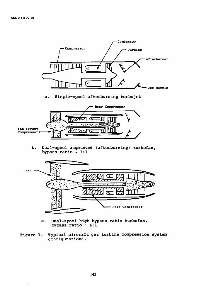
AEDC-TR-77-80
Compressor Turbine
/ - - - A f t e r b u r n e r
/~=- Jet N o z z l e
a. Single-spool afterburning turbojet
- ~ompressor
o
b. Dual-spool augmented (afterburning) turbofan, bypass ratio ~ 1:1
Fan
c.
Figure 1.
~ Rear Compressor
Dual-spool high bypass ratio turbofan, bypass ratio ~ 6:1
Typical aircraft gas turbine compression system configurations.
142
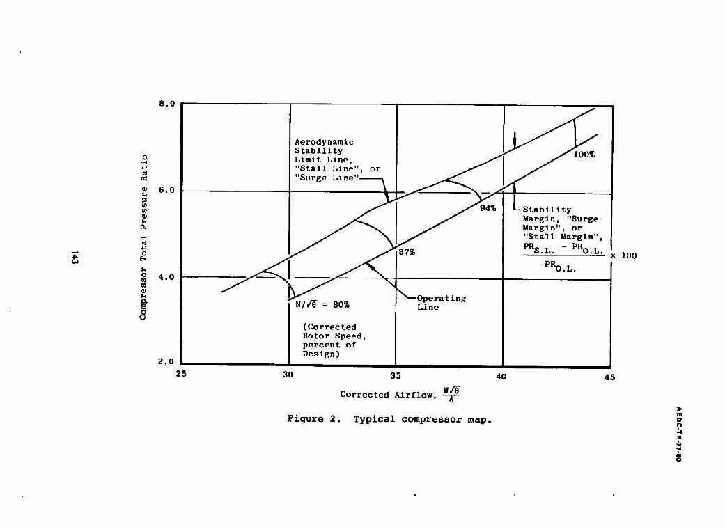
4~
8 . 0
0 .4 &J
n¢
¢ 6 . 0 S.,
r.4
0
o 4 0 .
E 0
2,0
25
J
Aerodynamic ~ 1 0 0 ~ % Stability Limit Line, / "Stall Line", or
. .
~--Operating N/~ = 80% Line
(Corrected Rotor Speed, percent of Design)
i
3 0 35 4 0 45
Corrected Airflow, W/e 6
Figure 2. Typical compressor map. m
.o -4
& o
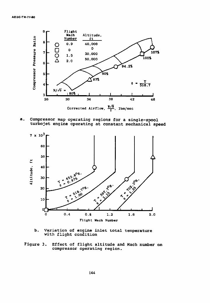
AE DC-TR-77.80
9 Flight .o Bach A l t i t u d e ,
Number f t ~ , ~
~ 8 o%7W-~ ~o--7~7~-- ~ A
== 1°s 3o,~oo = o,oo
8
3 1 80% I I , I , I , I 28 30 34 38 42 46
C o r r e c t e d Airflow ~W'v l b m / s e c ' 6
a. Compressor map operating regions for a single-spool turbojet engine operating at constant mechanical speed
7 x 10³-
60-- L
6 4 o - < ~0~,
"~ 3 0
0 ~ i , , / I , /, , , I 0 0 .4 0 . 8 1 .2 1 .6 2 .0
Flight Mach Number
b. Variation of engine inlet total temperature with flight condition
Figure 3. Effect of flight altitude and Bach number on compressor operating region.
144
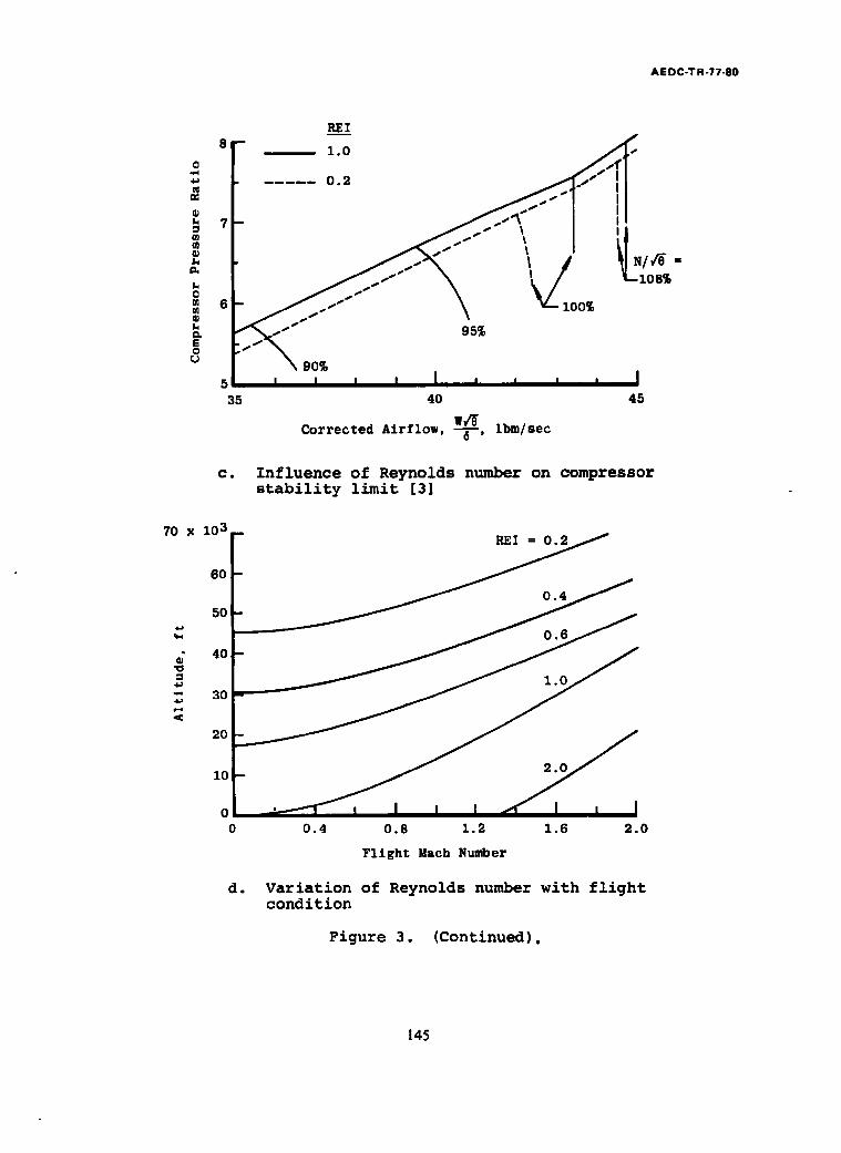
AEOC-TR-77-80
0
a
o
E o
8
6
5 35
REI
- 1 . 0
t-108%
0%
5%
\ 90% m i
i I i I I i i i i I 40 45
W/8 Ibm/sec Corrected Airflow, -~--,
c. Influence of Reynolds number on compressor stability limit [3]
70 x 103 r R E y
5 0
"~ 3 0
10
o ' I I i I / I ~ [
0 0 . 4 0 . 8 z . 2 z . 6 2 . 0
F l i g h t M a c h N u m b e r
d. Variation of Reynolds number with flight condition
Figure 3. (Continued).
145
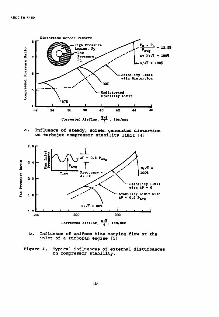
AEDC-TR-77-80
Dis to r t i on Screen Pa t te rn
8 -- ~ H i g h Pressure / ~ P H - PL -
o I//f ~ eeslon, P. / _~=~- -- = 12.5~ FX C~;'/A~Lo. / _s--, , ' ,
" T~'/A ~ " ~ / / / / / / / A Pressure / _~" s " " I at N//~ = 100~
6 -- / \ /~ "---Stability Li,-it / / ~ ~ with Dis to r t i on
~ . . . . / / / -
I ~ ~-- Undis tor ted / S t a b i l i t y Limit
87% 4
32 34 36 38 40 42 44 46
w~ Corrected Airflow, T ' lbm/sec
a. Influence of steady, screen generated distortion on turbojet compressor stability limit [4]
O ~4
m
k
W m
k
2.8
2.4
2.0
1.6
1.2 I00
|I _L ,~ o.., p,v,, / A
/ / ~ ~-- S t a b i l i t y Limit / / ~ ~ wlth AP = 0
f s ~" ~ ~ - S t a b i l l t y Limit with I ~ AP = 0.5 Pavg
N I / ~ = s0~ , , , , l I l l l I I I I I
200 300
Corrected Airflow, W#, lbm/sec
b. Influence of uniform time varying flow at the inlet of a turbofan engine [5]
Figure 4. Typical influences of external disturbances on compressor stability.
146
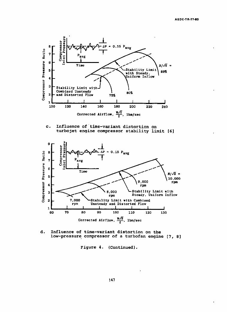
AEDC-TR-77-80
~I _L s , - ~ ~k-A--£~-~i-~-~p . 0.1s Pav
¢~ g o L = ~o~ avg
,, /.,,,, 3J-Stability Limit withJ ~ l
I Combined Uns teady | _ 80% 2 r and Distorted Flow 75%
,3 l / I I I I I I i00 120 140 160 180 200 220
C o r r e c t e d A i r f l o w , W ~ , l b m / s e c
I 240
c. Influence of time-variant distortion on turbojet engine compressor stability limit [6]
o 8 ~a
= 7
k
= 6
5
o 4 W
k 3 E o 2
d.
1 60
- / ~ - \ .... ~ io.ooo
_ ~ ~ ~ - - S t a b l l i t y Limit wi th rpm S t e a d y , Uni fo rm I n f l o w
7 ,000 S t a b l l i t y Limit wl th Combined rpm Unsteady and Distorted Flow
l I l I I I f 70 80 90 100 110 120 130
C o r r e c t e d A i r f l o w . W_~, l b m / s e c
Influence of time-variant distortion on the low-pressure compressor of a turbofan engine [7, 8]
Figure 4. (Continued).
i
147

AE DC-TR-77-80
3 . 6 vStability Limit w i t h \ S t e a d y Uni form I n f l o w
3.2 7 % / " \ \ w i t h Distort*on V ~ ' ~ \ \ and U n s t e a d y / .., '- \\ ~% I n f l o w from
~ 3 . 0 ~ " ./" \\ ~ Discharge of "~, ./*" \\ ~. U p s t r e a m
~ 2.8 ~, ~ I\; OmpressOr
~ 2.e ~\ ~ N/.~ = zo, soo rpm
o 2 . 4 %\% 10,000 rpm \
9 , 5 0 0 rpm 2 . 2 I I I I I
20 22 24 26 28 30
C o r r e c t e d A i r f l o w , W_~, l b m / s e c
e. Influence of unsteady and nonuniform flow from the low-pressure compressor on high-pressure compressor stability limit in a turbofan engine [8]
O
ee
L
~q
O
O
¢ L
E O
9
8
7
6
5
4 35
- ~ / L o w T e m p e r a t u r e Re g ion , T L / / / / / ~ (T H - TL) /Tavg = 19%
~ / ~ j r " H i g h T e m p e r a t u r e R e g z o n , T H _ ~ / ' ~ . . . _ g + o ~ ,
-- ~ " - - ~ t a b l l l t y L i m i t / ~ ~ wlth Unzform
t.. - ~ ' ~ - - ~ ' ' ~ . ~ " N / / '~ = 96.2% ~ . N/CO = 93.1%
- S t a b x l x t y Lzmi t w i t h Nonunzform T e m p e r a t u r e
K , z J I i , , , I 40 45
C o r r e c t e d A i r f l o w , ~ , l b m / s e c
f. Influence of nonuniform total temperature on a turbojet engine compressor [9]
Figure 4. (Continued).
148
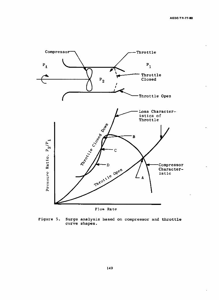
A E D C-T R-77 -80
C o m p r e s s o r - ~
~-~ \ ~
¢ 0 P2
s Throttle
~ - - - - ~ T h r o t t l e Closed
l l
Throt t le Open
Cq n.
d +J
o ~=
T..
Z'
/,
C
D
C
B
Loss Character- istics of Throttle
u o m p r e s s o r Character- i s t i c
Flow Rate
Figure 5. Surge analysis based on compressor and throttle curve shapes.
149
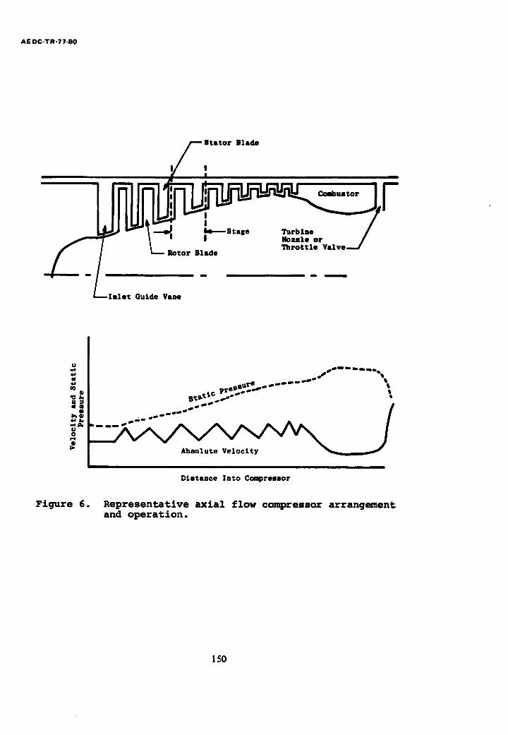
AE DC-TR-77-80
F 8tarot Blade
I I
F !
--'Y'------"-- --~lnletL Guide Vane -- --
U
eee-r'~- - ...... " / " ....... "~ ii ~ G VT ~ °° ee ° ' ' : el o o o I m l l b ° ° e ~ ° ° el'
D2ntance Into Compressor
Figure 6. Representative axial flow compressor arrangement and operation.
150
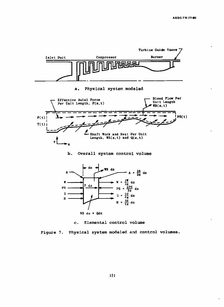
A E D C - T R - 7 7 - 8 0
Turbine Guide Vanes 7
Inlet Duct Compressor Burner /
a. Physical system modeled
~ p E f f e c t i v e Axial Force . ~ . B l e e d Flow Per er Unit Length, F(z , t ) UnitwB(z,t)Length
t P S ( t )
, _ . ,
#S ha f t Work and Heat Per Unit r ~ Length, WS(z,t) and Q(z,t)
z
b. Overall system control volume
_ _ ~ dz ~ ~ ~ _ _ _ _ _ BA A A + ~-~ dz
w __I=!F I V ~w PS dz _ L :- W + ~-~ dz PS ÷ ~--P~. dz
U =- U* ~--~ dz H : BH
H + ~-~ dz
W8 dz + Qdz
c. Elemental control volume
Figure 7. Physical system modeled and control volumes.
151
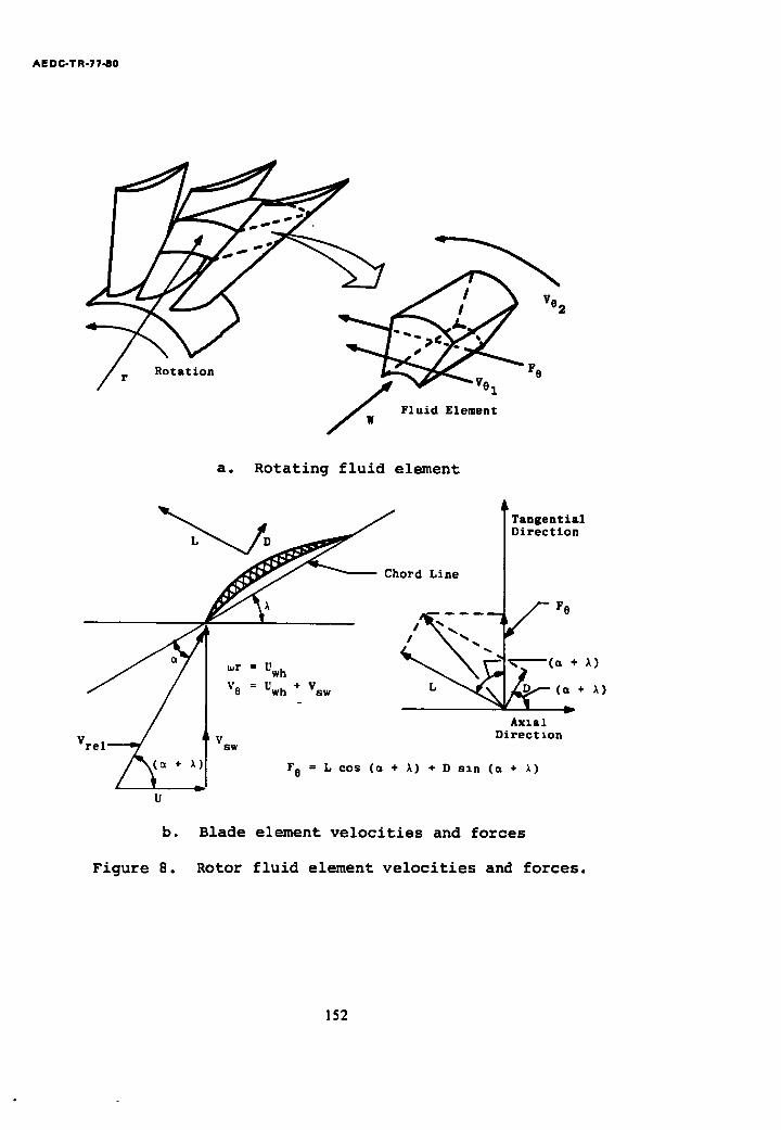
AE DC-TR-77-80
Ve 2
F e
Y 1
S F l u i d E lement
a. Rotating fluid element
hord L ine F8
V
U
mr = Uwh
V 8 = Uwh + Vsw
V sw
(a + ~)
Axlal Directlon
F 8 = L cos (a + A) + D sxn (a + A)
b. Blade element velocities and forces
Figure 8. Rotor fluid element velocities and forces.
152
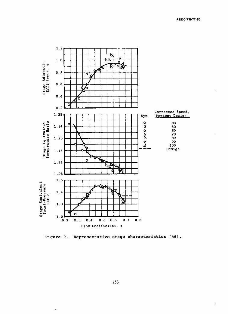
AEDC-TR-77-80
_~ :~,
, -
¢/2
~o
4~
~ c
o3
1.2
I 0
0.8
0.6
0.4
0.2
1 28
1 24
1 20
1 16
1 12
o~/
i 0
_ J
- - - - C
~ t
, !
" i Io
1 08
1.5 [ i
1.3 --. j ]
~.~ ~ 'o l I 0 . 2 0 . 3 0.4
_i [
I !
I
!
; I ,
I I i
~ N U
! l ' I
0.5 0.6 0.7
Flow Coefficient, ¢
Sv.~
O rl
O
V
m ~ m
0.8
Corrected Speed, Percent DesiEn
30 50 60 70 80 90
100 D e s z g n
Figure 9. Representative stage characteristics [46].
153
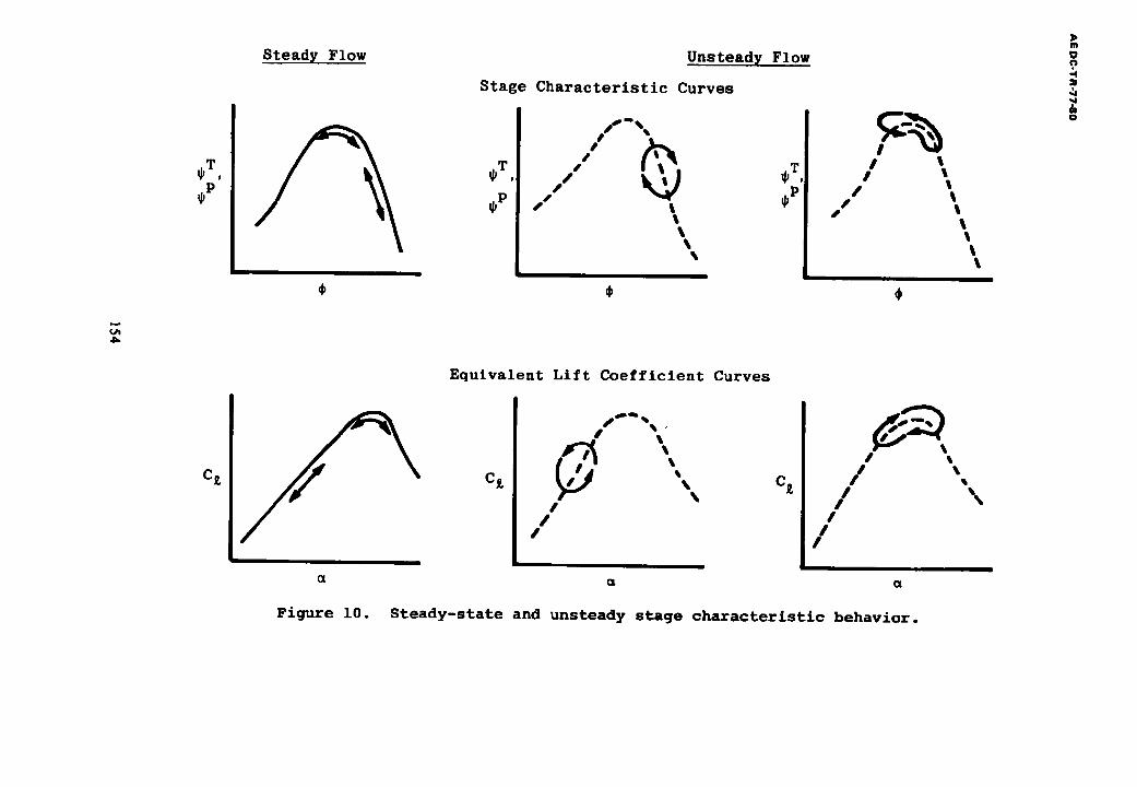
4a
Steady Flow
~P
Unsteady Flow
S tage C h a r a c t e r i s t i c Curves
~T
~P ss /
s Sp • l
l
~T, ~P
I I
l S
I I l 1 l 1 l l
E q u i v a l e n t L i f t C o e f f i c i e n t Curves
c~ c~ ~ c~ / \
/ /
Figure i0. Steady-state and unsteady stage characteristic behavior.
> m 0 ? "4
& O
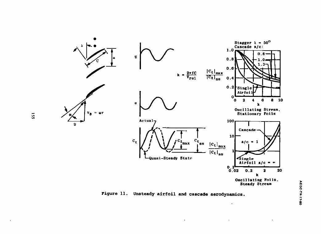
Stagger k = 50°I~. i ~ ~ _ ~ Cascade a/c : ~°~Io~
u o. S I - - ~ k \ X ¢ - 1.o
-- 0 ii 1 3~ k -- -_~._C Ic~l~x Vrel [Cllss 0
0"0 , - _ .
a ~ 0 2 4 k 6 8 I0
Oscillating Stream, Stationary Folls
k a[ r]
U Actua~ I00- l
T Y/? c 'V / ~J. '_c_" s. ..,........ r," .7- ~ , - . ~ ' L-quasi-Steady Stat(,
O. O. 02 O. 2 2 20
k Oscillating Foils.
Steady Stream
Figure 11. Unsteady airfoil and cascade aerodynamics.
m 0 9 -4
m 0

t , / t o~
I C ~ l m a x -r~-[-ss
1 . 2
1 . 0
0 . 8
0 . 6
0 . 4
0 . 2
0
0 . 0 2
On cP
[]
= 50 ° a / c = 1 , 3 - - X O
% B r u c e a n d H e n d e r s o n . 14B]
0 ~ = 4 s o a / ~ = 1 . ~ s 3 \ D X = 55 ° a / C = 1 . 3 5 3
=__c_c N o t e B r u c e and H e n d e r s o n D a t a k = V r e l N o r m a l i z e d t o A v e r a g e o f Co V a l u e s a t L o w e s t V a l u e o f k (% 0 .6 ~
C ffi F u l l B l a d e C h o r d L e n g t h
I I i I I I [ I I I I J i i i j I I I 0.04 0.06 0.1 0.2 0.4 0.6 1.0 2.0 4.0
k
I I I I I 6.0 10.0
Figure 12. Comparison of theoretical and experimental unsteady cascade lift coefficients.
m o n "4 3
& 0
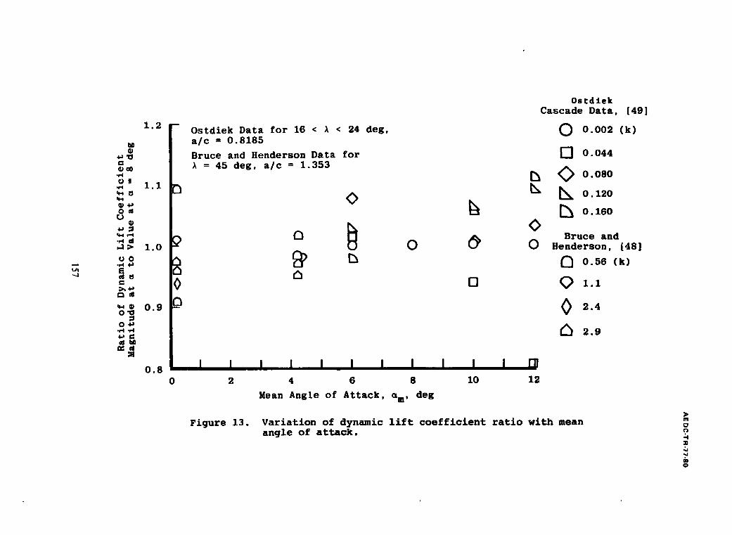
t ~
1 . 2
~00
OH 1.1
oe o
• ,4 d ~ 1.0 o o
• , 4 4-~
t ~ e l
~ 0 . 9 O ~
O ~ • , 4 . - I
G d ~
0 . 8
O s t d 2 e k D a t a f o r 16 < Z < 24 d e E , a / c = 0 . 8 1 8 5
B r u c e and H e n d e r s o n D a t a f o r = 45 d e g , a / c = 1 . 3 5 3
<>
O
O s t d i e k C a s c a d e D a t a , [49 ]
0 0 . 0 0 2 ( k )
D 0.044
[~ ~ O. 080 I',, ~ o .12o
C3 o,1 o <>
B r u c e a n d ( ~ 0 H e n d e r s o n , [ 48 ]
E]
0 . 5 6 ( k )
1 . 1
2 . 4
2.9
0
I I
2
Figure 13.
I l . I I I I 4 6 8
Mean A n g l e o f A t t a c k , ~m' d e g
10 12
Variation of dynamic lift coefficient ratio with mean angle of attack.
m
o 0
~s
m 0
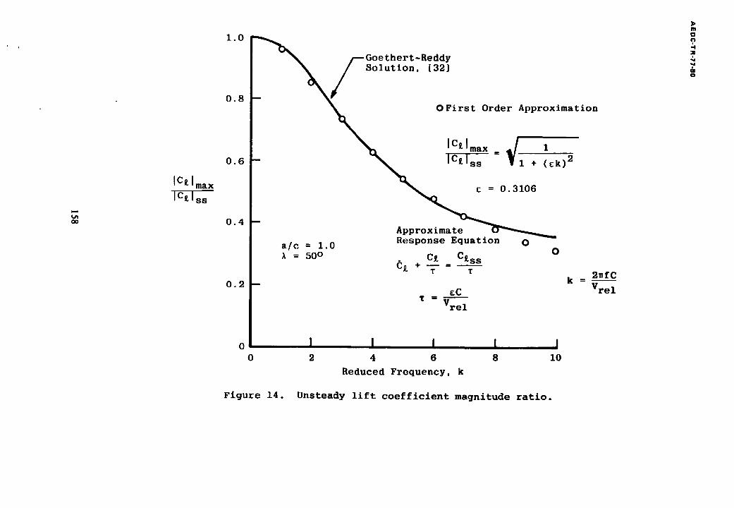
1 . 0
G o e t h e r t - R e d d y S o l u t i o n , [ 32 ]
fll
~3 ?
& 0
0 . 8 O F i r s t O r d e r A p p r o x i m a t i o n
IC£[ma x
IC~Iss
0 . 6
0 . 4
0 . 2
0
Ic~{max = . f IC~lss ~ 1 + ( e k ) 2
e = 0 . 3 1 0 6
A p p r o x i m a t e a a / c = 1 . 0 R e s p o n s e E q u a t i o n
A ffi 50 ° C£ C£ss ~ + -- =
T T
eC T = Vrel
0 0
k = _ _
I I I I 2 4 6 8
R e d u c e d F r e q u e n c y , k
10
2 . f C
V r e l
Figure 14. Unsteady lift coefficient magnitude ratio.
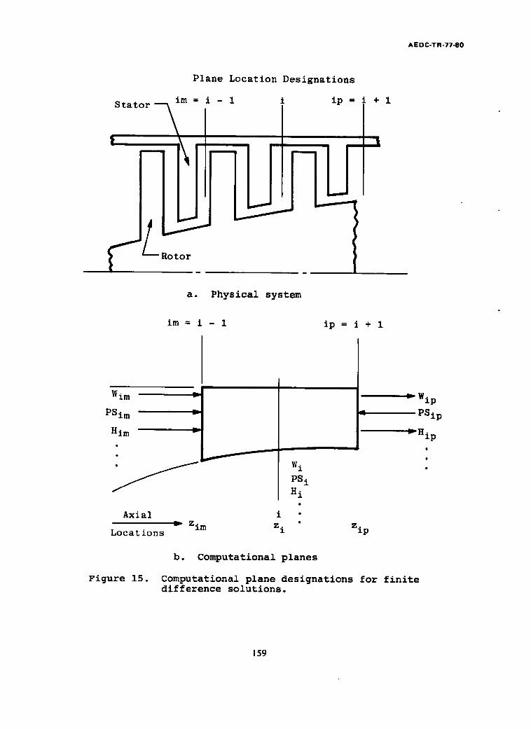
AEDC-TR-77-80
Plane Location Designations
im = i - 1 Stator--~
t m
q
C/_.o.o. /
ip= i +I
-A
a. Physical system
ira=i- 1 ip= i + 1
Wim
PSi m
Him
v
v
W i PS i H i
Axial i • Z • v im z. z.
Locations m l p
Wip
P S i p
Hip
b. Computational planes
Figure 15. Computational plane designations for finite difference solutions•
159
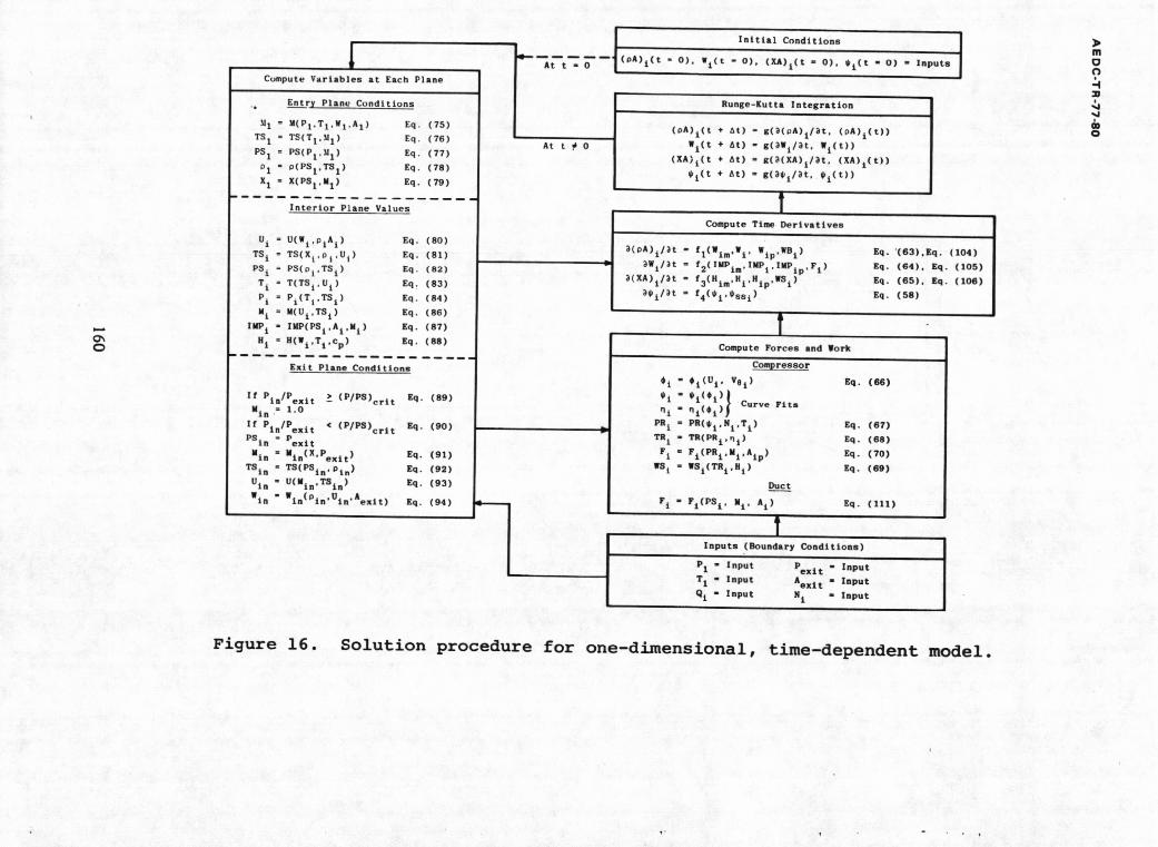
0
Cumpute V a r i a b l e s at Each P lane
• , Entry Plane C o n d i t i o n s
U I " M(PI,TI.WI.A I ) Eq. (75) TS 1 • TS(TI.U 1) Eq. ( 7 6 )
PSI = PS(P1,M 1) Eq. ( 7 7 )
o I = o(PSI ,T81) Eq. (78) XI i X(PSI.MI ) Eq. ( 7 9 )
I n t e r i o r Plane Values
UI i U(Wl,01AI) Eq. (80) TS i " T S ( X i , 0 | , U i ) Eq. (81) P5 i = PS(oi ,TS I ) Eq. (82)
T i " T(TSA,U I ) Eq, (83)
Pl = P i ( T i ' T S I I Eq. (84) M i " M(UI,TS i ) Eq. (86)
IMP i - IMP(PSI.Ai.M i ) Eq. (87)
8 i = B ( g i , T i . c p) Eq. (88) m m m m m m m ~ N m m N m m m m m r a m ,
E x i t P l ane C o n d i t i o n s
I f P i n / P e x i t ~ ( P / P S l c r l t Eq. (89) Min .- 1 .0
I f P l n / P e x i t < ( P / P S ) c r l t Eq. (90) PSin ~ P e x i t
Min = Min(X.Pex i t ) Eq. (81) TSin " TS(PSin. Oin) Eq. (921
Uin = U(Min,TSln) 8q. (93)
g in " g i n ( O i n ' U i n ' A e x l t ) Eq. (94)
At t - 0
At t ~ 0
I n i t i a l C o n d i t i o n s |
l ( o A 1 i ( t i 01, W i ( ; ' - 01, (XA1i( t = 01, * i ( t - 01 " lnpu
Runge-Kuttn I n t e g r a t i o n
I
( P A ) i ( t + At) = 8 ( a ( p A ) l l | t , ( p A l l ( t ) )
| i ( t ÷ At) - 8 ( a V i l a t . g l ( t l ) (XA)l(t + A t ) - 8(~ (XA) l /~ t , (XA11(t11
$ i ( t + At) - f ( ~ $ i / ~ t , O l ( t ) )
T Compute Time D e r i v a t i v e s
] a ( o A ) i / ~ t - f l ( g i m , W i , Wip.WB i )
~wi /~ t = f2(IMPim, IMPi. IMPip 0F i ) ~(XA) I /a t - f 3 ( H i m , H f . H i p . g S l l
~ e i / a t = t 4 ( e i . $ n n l )
T Compute Forces and gork
Compressor
# i " # i ( U i ' Va i l e i - e l ( I l l ~ q l n i ( t i ) } Curve F i t s
PR i = P R ( e i . N i . T l ) TR i - T R ( P 8 1 . , i )
Y 1 = F i ( P R i . l i , A i p ) 88 i - gSi(TRA,HI)
Duc___~t
F i = Fi(PSi, M i, A i )
Eq. "(63) ,Eq. (104) Eq. ( 6 4 ) . Eq. (105) Sq. ( 6 5 ) . Kq. (1081 Eq. (581
• qo ( e e )
Eq. (67) Eq. (68) Eq. (701 8q. ( 8 9 )
Eq. (111)
I n p u t s (Boundary C o n d i t i o n s )
P l i Inpu t P e x i t = Inpu t
T 1 " Inpu t A e x i t = I n p u t Qi i Inpu t N l o Inpu t
m o ?
& 0
Figure 16. Solution procedure for one-dimensional, time-dependent model.
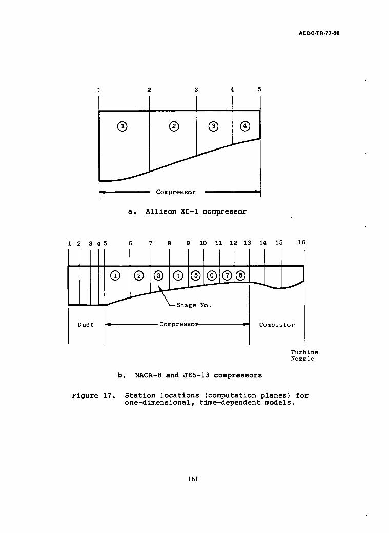
AE DC-T R-77-80
1 2 3
® ®
J
4 5
® ®
Compressor
a. Allison XC-I compressor
1 2 3 4 5 6 7 8 9 I0 11 12 13 14 15 16
@
Duct I_
Turbine Nozzle
b. NACA-8 and J85-13 compressors
Figure 17. Station locations (computation planes) for one-dimensional, time-dependent models.
16l
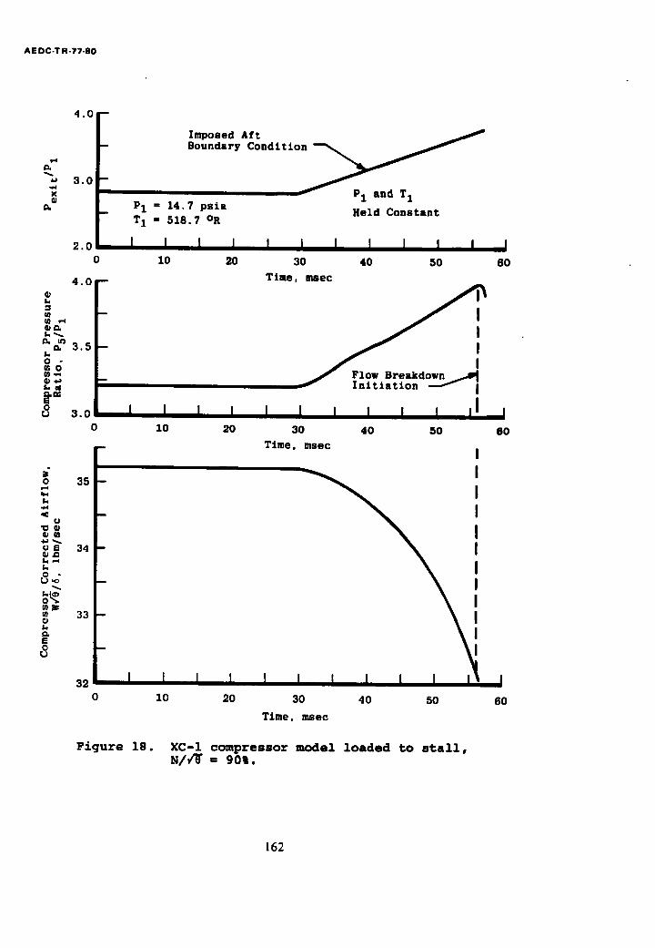
AE DC-T R-77-80
4 . 0
~ 3 . 0 -
GI
2 . 0 0
4.0 m
k
M
k ~
= 3.5--
o - o
L t
o o 3 . 0
0
o 35 -
~ m
u s 34 --
k o -
33 --
E O
32
0
P l = 1 4 . 7 p s L a
T I = 5 1 8 . 7 OR
t I I i 10 20
I I I 10 20
I I I I I 10 20
P l a n d T 1
H e l d C o n s t a n t
I I I I I I I I 30 4 0 50 60
TLme, msec
/ F l o w B r e a k d o w n ~ " I n L t t a t L o n ~ i
I
I I I ] I I I' I 30 40 50 60
Time, msec [
[
!
I I i I I I ~ I 30 40 50
TLme, m s e c
Figure 18. XC-I compressor model loaded to stall,
N//~= 9 0 % .
6 0
162
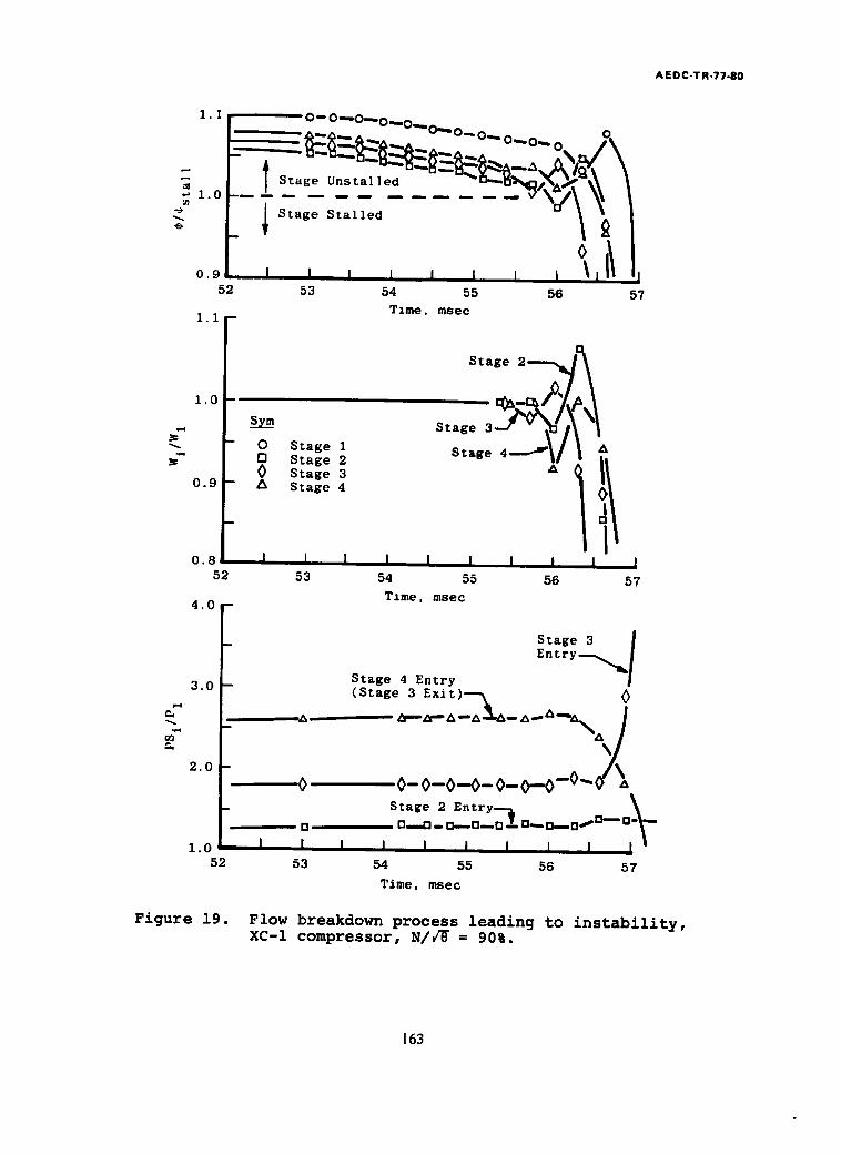
AEDC-T R-77-80
o,
j ~.oI-- t . . . . . . . . . . - ~ \ ~
52 53 54 55 56 57 Time. msec 1.1-
1.0
0 .9
s ~
- O Stage 1 Q S tage 2 0 Stage 3
-- ~ S tage 4
0 .8 I I 52 53
4.0 m
Stage 2 ~ 1 t _ _ ~ / O ~ /
I I I I l I I 54 55 56 57 Time. msec
3.0
2.0
0
o
1.o i I I 52 53
Stage 3 I
Stage 4 Entry Entry~/
(S t age 3 E x i t ) - - ~ 0
O- 0-0-.0_ O_ 0.-0-0-- 0/~ Stage 2 E n t r y - - ~ ~ .~._ D___~__O.__O.__DImD..O.__D~D O-~
I I I I I I ~ ' 54 55 56 57 Time, msec
Figure 19. Flow breakdown process leading to instability, XC-1 compressor, N//~ = 90%.
163
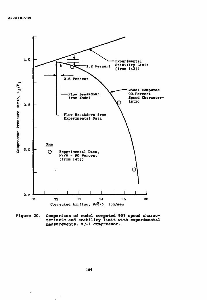
AE DC-T R-77-80
4 . 0
1-4
J qq 4~
3 . 5
¢1
1,4
$4 0 W
o 3 .0
2.5
i ~ r p e r c e n t lmental , ~ Stability Limit (from [43])
- - - - - - . 4 m
-- I 0.6 Percent
~----Flow Breakdown from Model
Model Computed 90-Percent Speed Character- istic
Flow Breakdown from Experimental Data
sym
0 Experimental Data, N/~/e = 90 Percent (from [43])
C
31
I I I I 1 I I I I J 32 33 34 35 36
C o r r e c t e d A i r f l o w , Wv~/6, l bm/sec
Figure 2 0 . Comparison of model computed 90% speed charac- t e r i s t i c and stability limit with experimental measurements, XC-I compressor.
164
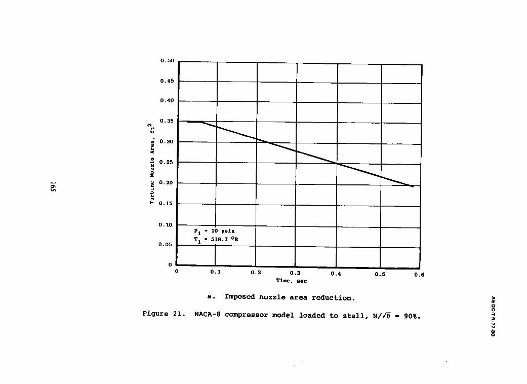
0.50
tn
0.45
0 . 4 0
0.35 t ~
=~ 0 . 3 0
,==
• -~ 0 . 2 5 N N O
Z
® 0 . 2 0 ,4
JD k ,
[ - 0 . 1 5
O . 1 0
0.05
--- . . . .
P l = 10 p s l a
T 1 - 5 1 8 . 7 ° R
0 . 1 0 . 2 0 . 3 0 . 4 0 . 5 0 . 6 T l m , sec
Figure 21.
a. Imposed nozzle area reduction.
NACA-8 compressor model loaded to stall, N/~ = 90%.
m o O
& O
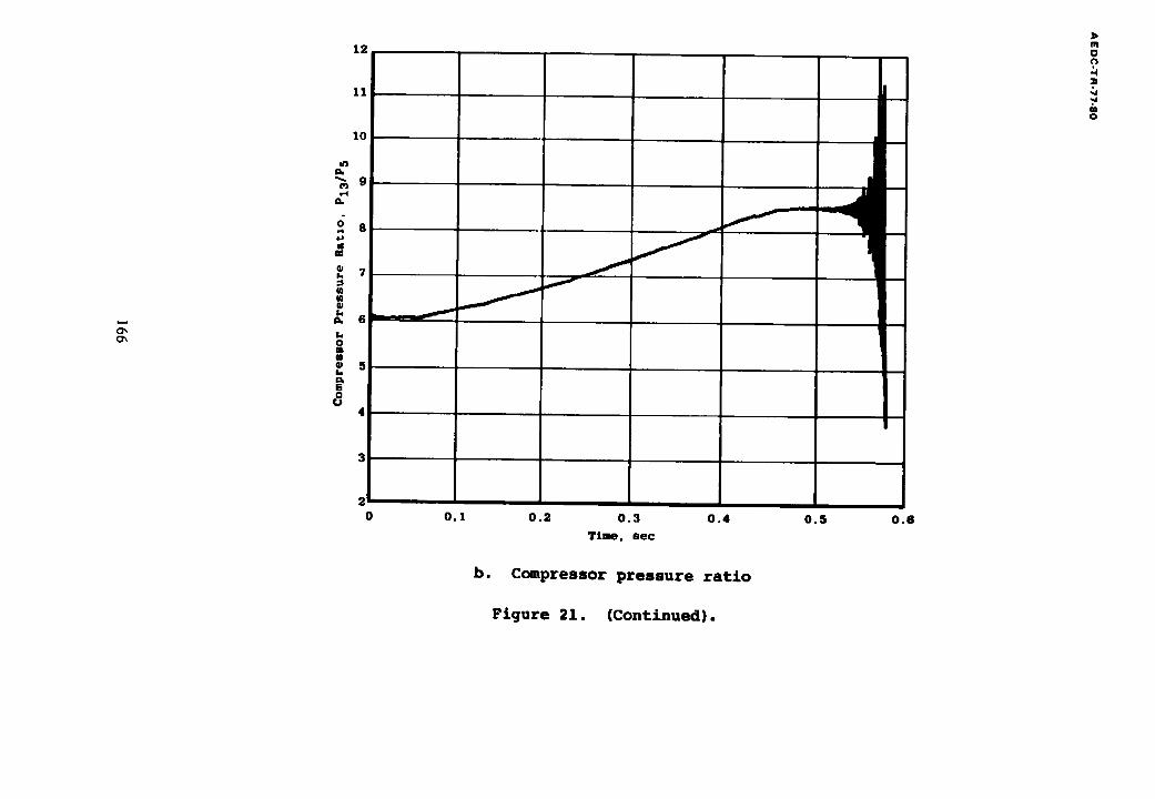
1 2
1 1
1 0
dl n.
"A 9j e..4
n .
1'4
g
~ 7 k I
GO III fO J4 ~ _ _
A. 6
h 0 B m 0 '-- I
[] 0
U 4 '
3
2
J
J i
f
I J
I I
0 . 1 0 . 2 i i
0 . 3 0 . 4 0 . 5 0 . 6
T i m e , Bec
b . Compressor pressure ratio
Figure 21. (Continued}.
m O
& O
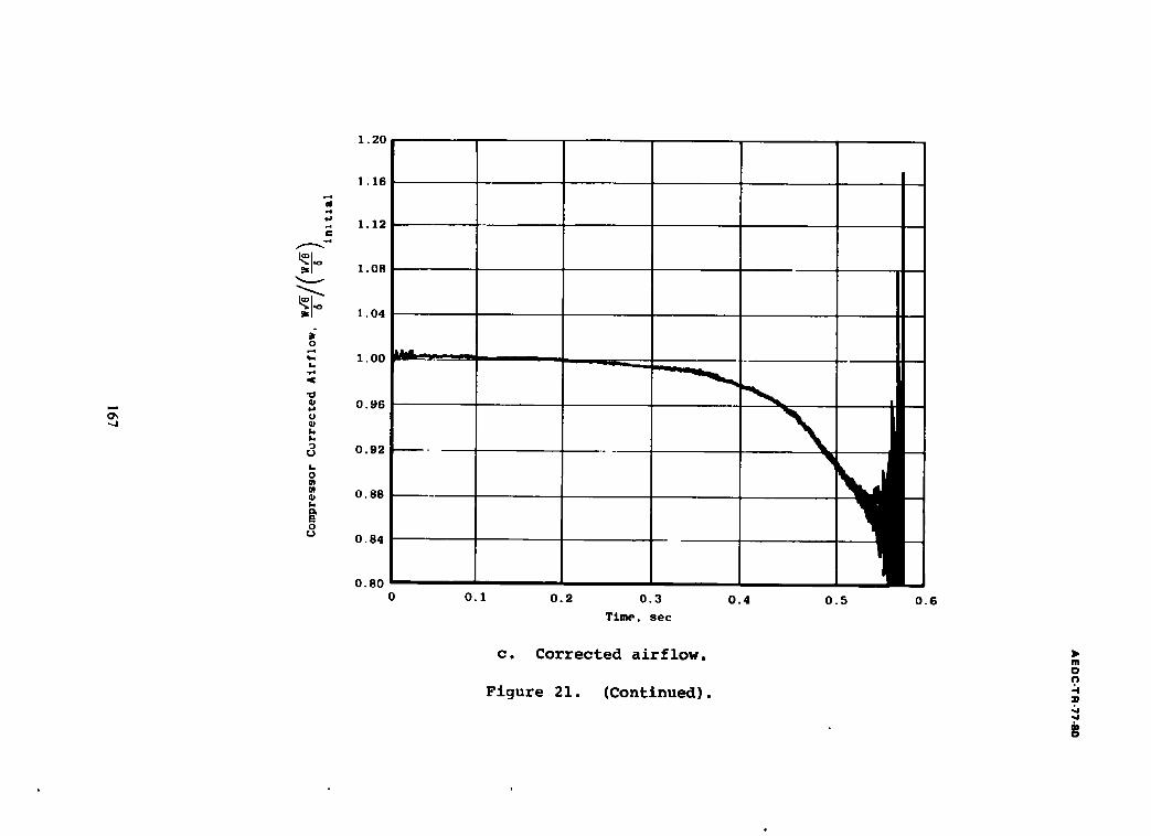
1.20
O~ -,3
,.4 4~
~1 ~
o ,...4
4J
Q;
k 'D
r j
k o
w
o,
o (.)
] , 1 6
1 . 1 2
1 . 0 8
I , 0 4
1 . 0 0
0 . 9 6
0 . 9 2
O , 8 8
\
0 . 8 4
I II H |
0.80
0 0.I 0 . 2 0 . 3
Time, sec
c. Corrected airflow.
Figure 21. (Continued}.
0.4 0.5 0.6
m O
~s
00 o
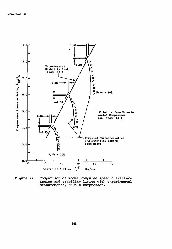
A E D C-T R-77-80
9 . 0 m
8.0 --
I
7 . 0 -
n .
B
a 6 . 0 -
L
m Ui 0
~' 5 . 0 - h 13
10 - - qo L. eL
E 0 4 . 0 -
3 . 0 -
2 .0 2O
Figure 22.
E x p e r i m e n t a l S t a b i l x t y Limit ( f r o m [45] )
2.2% - - - ~ "
,1 L.~ ~,
#
T'-'II'-/
t'-~/~°~ °
L o 0
0
0 0
OoN/~ = 90%
°o 0 P o i n t s f rom E x p e r i -
m e n t a l Compres so r map ( f r o m [45] )
Computed C h a r a c t e r i s t i c s and S t a b i l i t y Limits f rom Model
11 °
I I I I I I I 30 40 50 60
w ~ C o r r e c t e d A i r f l o w , T ' I b m / s e c
I j 70
Comparison of model computed speed character- istics and stability limits with experimental measurements, NACA-8 compressor.
168
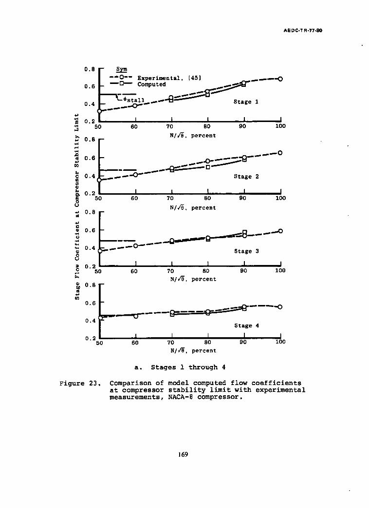
AE DC-T R-77-80
0 . 8 [ -
| - - - 0 - - E x p e r i m e n t a l , [45] ~ . . . - - - - - - 0 L - - 1 3 - - " Computed _ _ ~ ~ o. s, , L - - - - -
0 .4 L - x- s t - - a l l - ~ - ' ~ ~ s t a g e 1 p_-- '~ o . 2 ~ I i I I I • ~ 50 60 70 80 90 100
i 0 8 F N/ /~ . p e r c e n t
/ ~ ~ 0
- - 0 4 . - - 0 " S t a g e 2
= 0 2 l I I I I I s 50 60 70 s o s o z o o 0
~J N/4e, p e r c e n t -~ 0 8 -- ed
4J
~ 0 6
~ 0 4 0 0
0 . 2 c 50
~ 0 . 8 -
D
~ " " " S t a g e 3
I I I I I 60 70 80 90 100
N/V~, p e r c e n t
0.S -- _--n-------~---~~------~ ~ - - - - - - u -- - - - - - ~ - -
0.4 S tag e 4
0 . 2 I I 1 i I 50 60 70 80 90 100
N/V~, p e r c e n t
a. Stages 1 through 4
Figure 23. Comparison of model computed flow coefficients at compressor stability limit with experimental measurements, NACA-8 compressor.
169
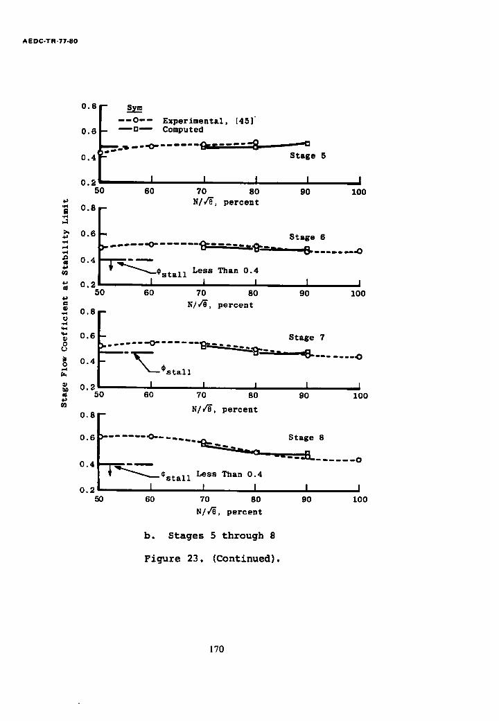
A EDC-TR-77-80
0.8 - s_~
- - - - 0 - - - - E x p e r i m e n t a l , [ 4 5 ] 0 . 6 - - - u - - Computed
.~o~..~. ...... ~. ...... .-° ~-~ 0 . 4 S t a g e 5
o . ~ I I I I I 50 60 70 80 90 100
N/a, p e r c e n t 0 . 8 ~
0 . 6 S t a g e 6
• r ~--'~=~---'~ .......
0 " 4 1 ~ " ' - - ¢ s t a l l " " - - - - L e s s Than 0 . 4
0 . 2 / [ I I ] I 50 60 70 80 90 I00
= N / a , p e r c e n t 0.8- - O ~4 qq
0.6
~o 0.4 -...4)
0.2 [ a 50 100 4a
G3
-- , S t a g e 7
~ - " - u - - = ~ - - - - ~ . . R .
- --'~¢stall
I I I I 60 70 80 90
N / / e , p e r c e n t O.S -
0 . 6
~ ¢ s t a l l I
60
S t a g e 8
-- w ~ m m ~ R D m m i m 0 0 . 4
L e s s Than 0 . 4
0 . 2 I I I I 50 70 80 90 100
N/V~, p e r c e n t
b. Stages 5 through 8
Figure 23. (Continued).
170
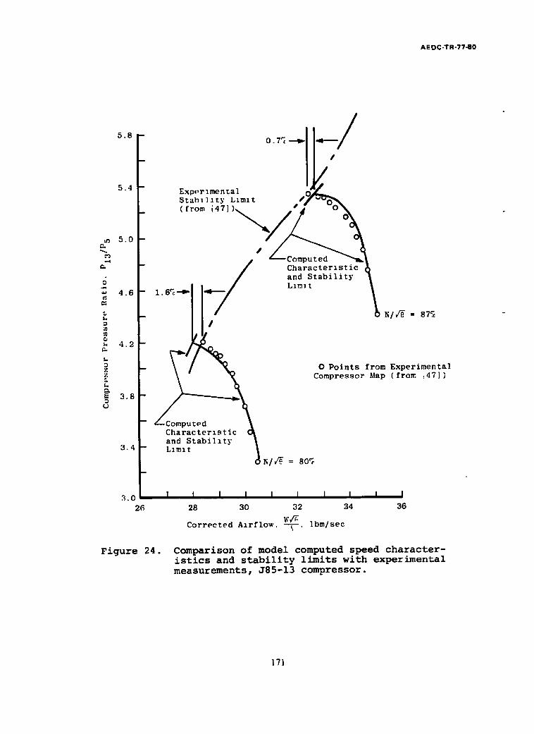
AEDC-TR-77-80
5 . 8
5 . 4
5 . 0 -
4 . 6 -
¢ L
if)
4.2 - - C .
L
D
L
~- 3 . 8 -
3 . 4 -
3 . 0
2 6
/ S~an111ty Ll.mz t / F ~
~ / Characterlstic
N / d ' ~ = 8 7 ~
O Points from Experimental Compressor Map (from ,47])
Computed Characterxstic and Stabillty L]mlt
~ / ~ = 8o~
i I I I I I I I l 28 30 32 34 36
~'~ Corrected Azrflow. - - - ' q - . . Ibm/sec
Figure 24. Comparison of model computed speed character- istics and stability limits with experimental measurements, J85-13 compressor.
171
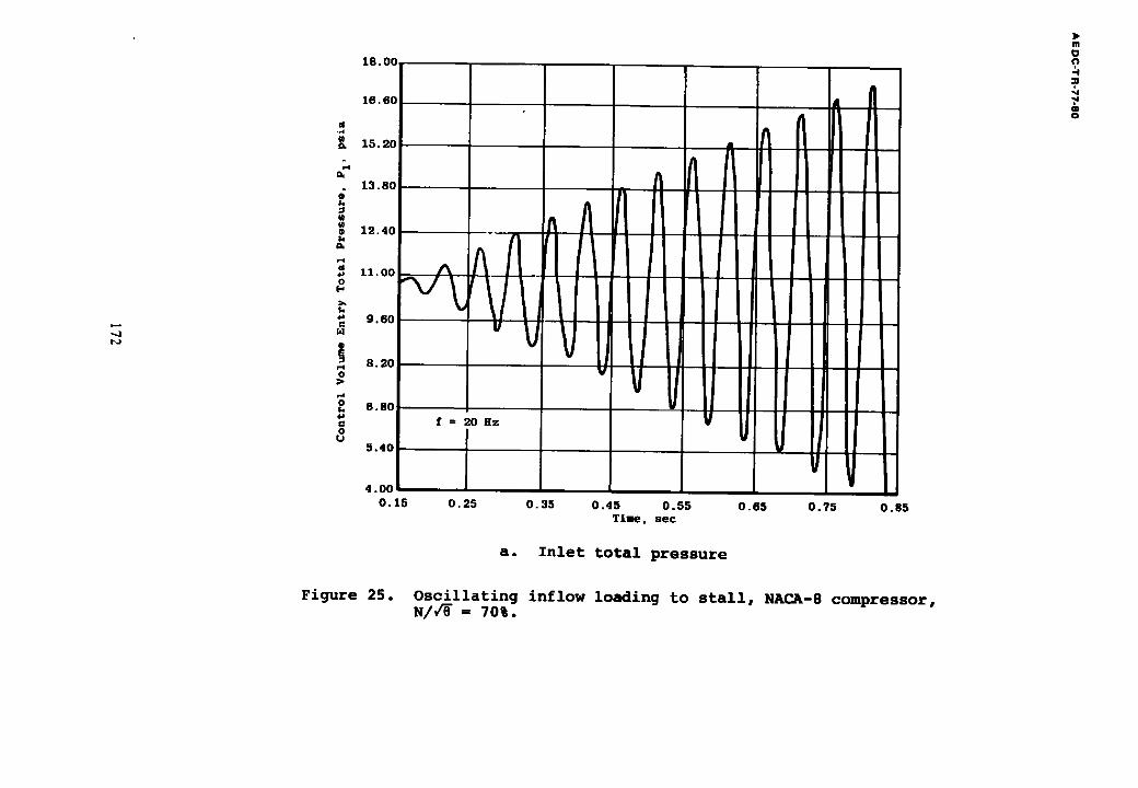
1 8 . 0 0
1 6 . 6 0 ] l,n IA n lll w
15.20 A ' I
i ~ 10 , in/I ~i II II ~,,..,o ~ ~ II I 1 !1 II II., - ' " . .
~ ,,.oo , , A f I I l . . l l l l l l l . . "" ~, \i I l l Ill II lal " 9 . 6 0 . .
, v ~ I l l i1111 IIII 8 . 2 0 • • , ,
u I/I lit II Illl "~ 6 . 8 0 • ,, , , _
~ uilJ i/ii - , f : 2 0 H z O
U 5 . 4 0 . .
.oo 1 v l l 0 . 1 5 0 . 2 5 0 . 3 5 0 . 4 5 0 . 5 5 0 . 6 5 0 . 7 5 0 . 8 5
TAme, s e ¢
a. Inlet total pressure
m
0 ?
~ J
oo o
Figure 25. Oscillating inflow loading to stall, NACA-8 compressor, ~I/~= 7 o ~ .
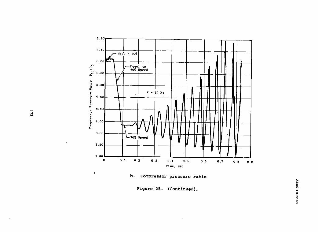
%
J.J
o
6,80
6 . 4 0
i~ O0
rj. 60
5.20
4 80
4 . 4 0
4.00
2.80s 0
i~N//O = 9o% I , - - -Dece] t o
70% Speed
!
f = 20 Hz
-l ;
~" 70%ipeed
O. 0.2
/I/
0 3 0 . 4 0 . 5 0 6
Time, $ec
0.7 0 8 09
b. Compressor pressure ratio
Figure 25. (Continued).
> m o
~4 & 0

--.I
1 O0
O. 90
0.80
~o7o
0 GO
o . 50
.7
k .~ O. ,10
t. 0 3 0
k
E 0 O . 2 0
0 . 1 0
0 0 1 5
nP *I
Ill II Ill II II II/
f - 2 0 I I z
ItlllIJ
V, 0.25 0.35 0.45 0.55 0.65 0.75 0.85
Time, sec
c. Compressor entry airflow
> m o n
m o
Figure 25. (Continued).
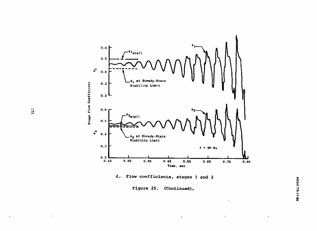
..j ta-,
0.6 01 I
0.5 1 0 . 4
~ 0 . 3 / S t a b i l i t y L i m i t
l ~, o . s
: .- 0 . 4 - 0 2 a t S t e a d y S t a
S t a b i l i t y L i m i t
0 . 3 - f =
0 . 2 I I I , I I ., I I O. 15 0 . 2 5 0 . 3 5 0 . 4 5 0 . 5 5 0 . 6 5 0 . 7 5 0 . 8 5
Time, se¢
d. Flow coefficients, stages 1 and 2
Figure 25. (Continued).
m O
~J & O
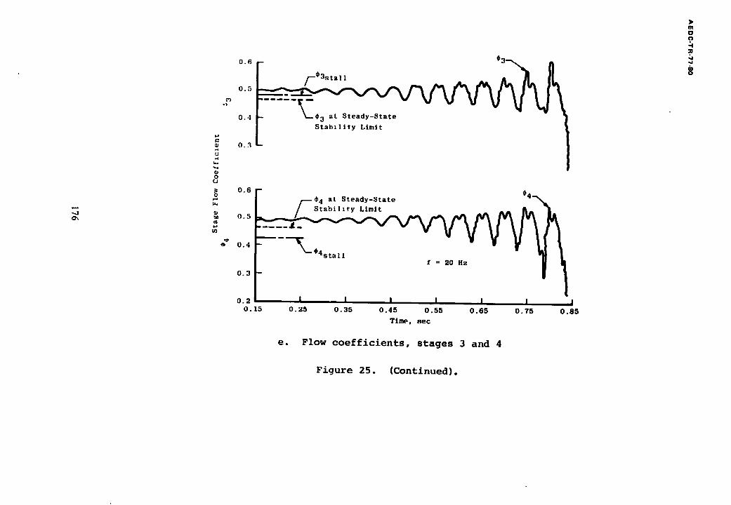
.,.j
0 .6 %3
0.5 .P
O.,l
~ 0.3
o (J
0.6 ~ %4 / " - ~ 4 at Steady-State - ' ~
0.5 u)
0.4
0.3
0 . 2 1 I i I I , I I ~1 O. 15 0 . 2 5 0 . 3 5 0 .45 0 .55 0 . 6 5 0 . 7 5 0 . 8 5
Time, Rec
e. Flow coefficients, stages 3 and 4
> m O ? 3
m O
Figure 25. (Continued).
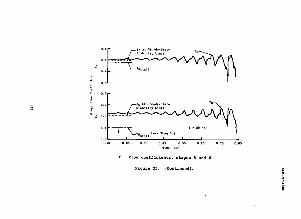
~4 ..j
0.6[-- ~ ' 5 at S teady-S ta te , I / Stabl I tty Limit 5 - - ' ~ _
0.5
0.4
0.6 / " - -*6 at S t eady-S ta t e 6~_
e6s t~ l l Less T:an 0 . 3 I I O. 15 0.25 O. 35 0.45 0.55 0.65 0.75 0.85
Time, sec
f. Flow coefficients, stages 5 and 6
Figure 25. (Continued). > m 0 n
$
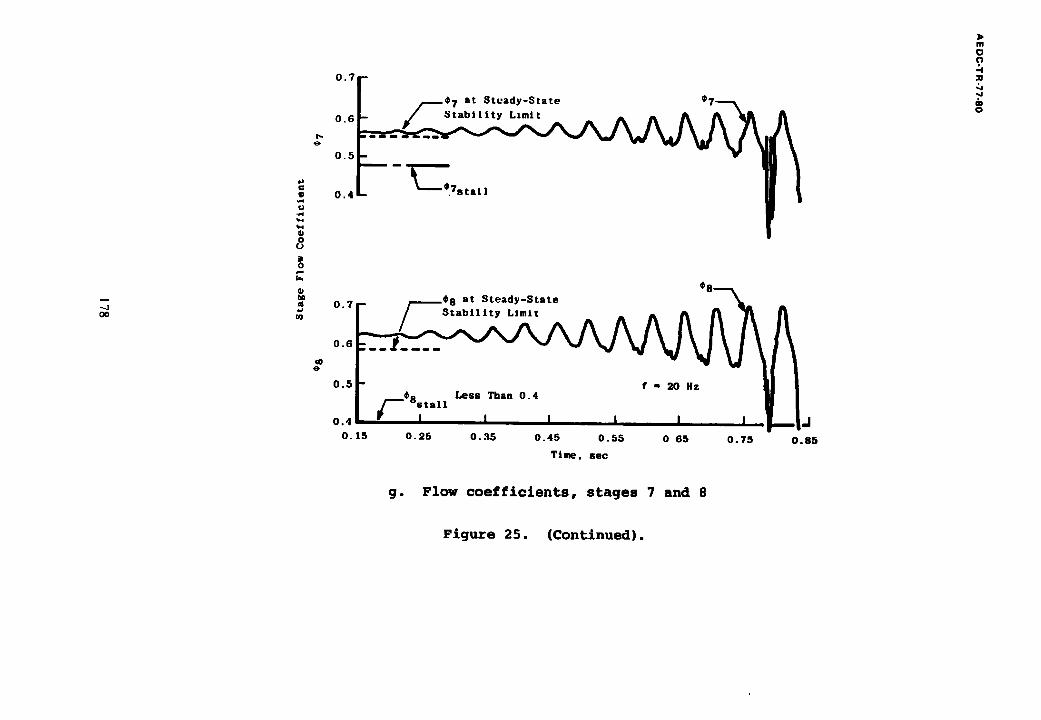
oo
u
o
0 . 7
0 , 6
0 . 5
0 . 4
~p --@7 a t S t e a d y - S t a t e S t a b i l i t y L s m i t
. 7 s t a l I
0S 0 . 7 - - ,_. . . . . . .0 s a t S t e a d y - S t a t e ~ .
~o / S t a b i l i t y L i m i t
0 . 6
0 . 5
0 . 4 d 0 . 1 5 0 . 2 S 0 . 3 5 0 . 4 S 0 . S S 0 65 0 . 7 5 O .S5
T ime . s e c
m O n
m o
g. Flow coefficients, stages 7 and 8
Figure 25. (Continued).
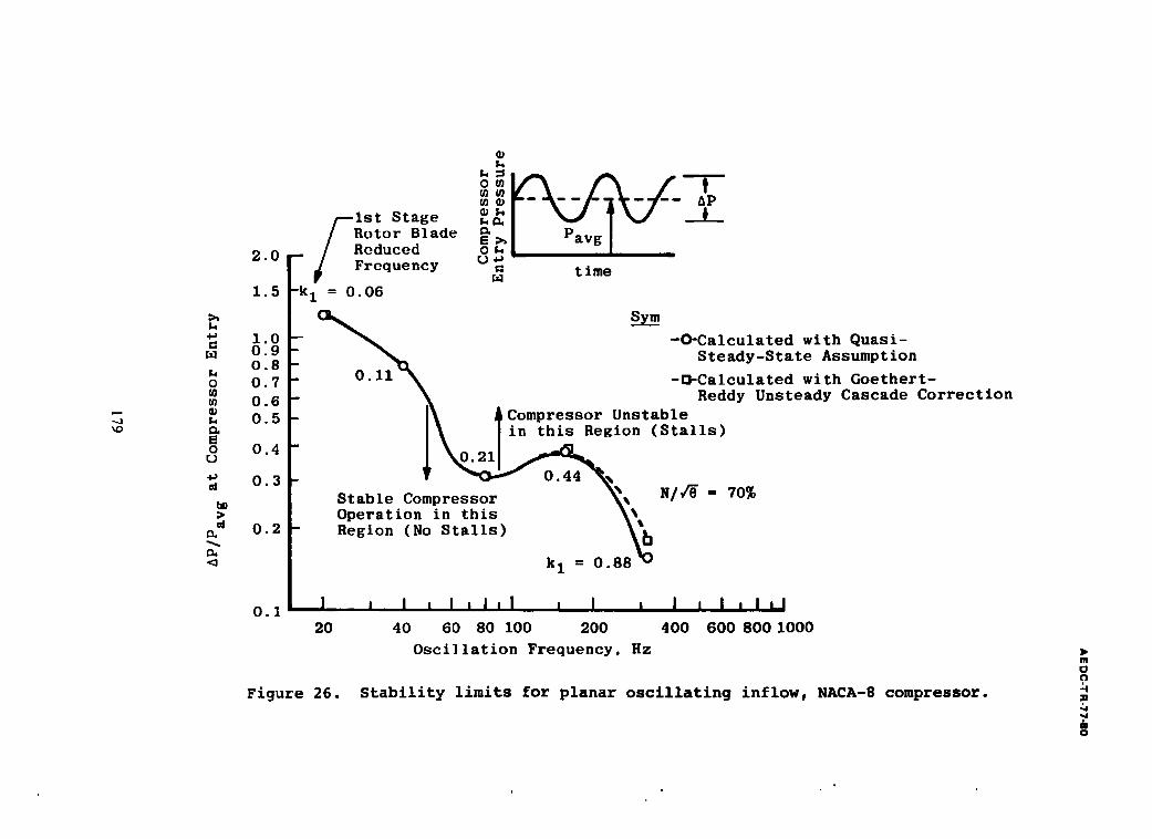
~D
+J
O
O U
4~
~0
¢d
2.0
1.5
1.0 0.9 0.8 0.7 0.6 0.5
0.4
0.3
0.2
0.1
A 1-7-
/Rotor Blade /Roduced ~Frequency ~ time
-k I = 0 . 0 6
- ~ - O - C a l c u l a t e d w i t h Q u a s i - Steady-State Assumption
0.11~ -Q-Calculated with Goethert- Reddy Unsteady Cascade Correction
I\ $ Compressor Unstable I ~ / i n this Region (Stalls)
Stable Compressor ~ NI 4~ = 70% O p e r a t i o n i n t h i s ~ Reglon (No Stalls) ~b
I,, k I = 0.88 v
I , | , I , I i I , I , I I I , I , I
20 40 60 80 100 200 400 600 800 1000
Oscillation Frequency, Rz
Figure 26. Stability limits for planar oscillating inflow, NACA-8 compressor.
m o o -4
q4 & o
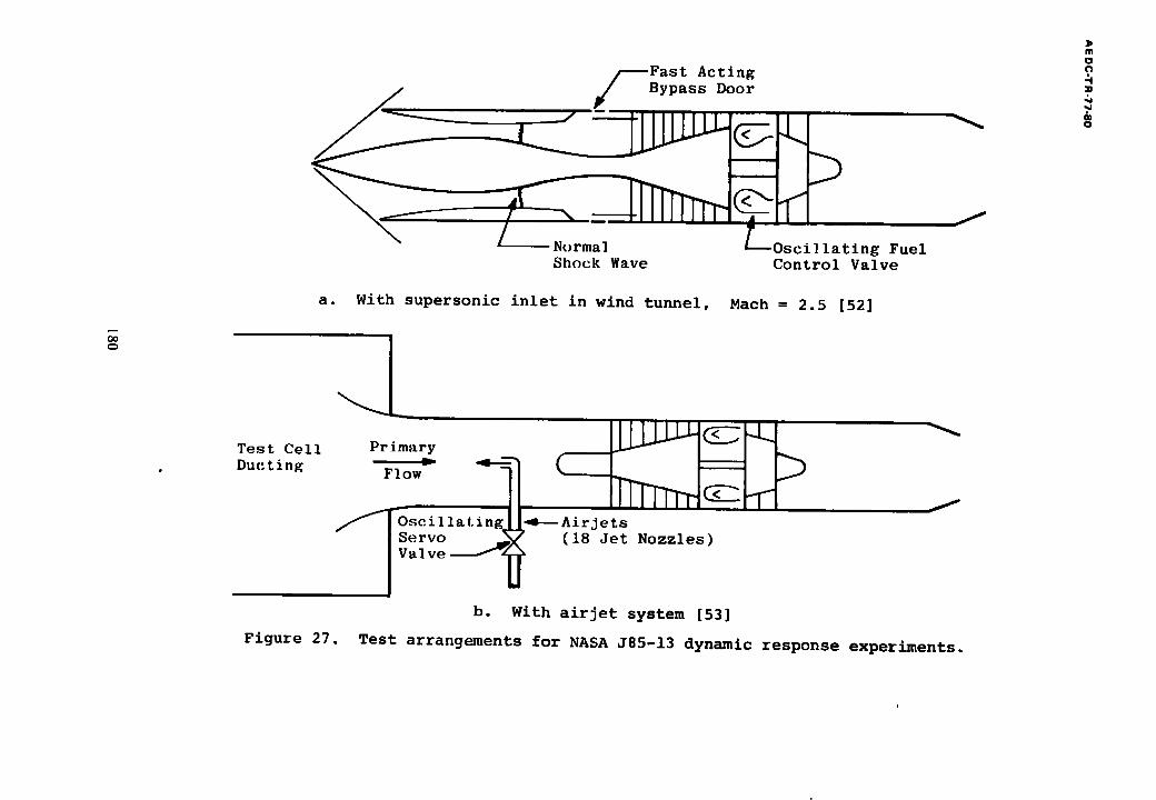
CD
f Fast Acting Bypass Door
~ ====_=====~L=_~,,,,~,, J L''
--Normal Oscillating Fuel Shock Wave Control Valve
/
a. With supersonic inlet in wind tunnel, Mach= 2.5 [52]
Test Cell Ducting
Primary . L ~ ~ ~ "j~
b. With airier system [53]
i
m O o
& O
Figure 27. Test arrangements for NASA J85-13 dynamic response experiments.
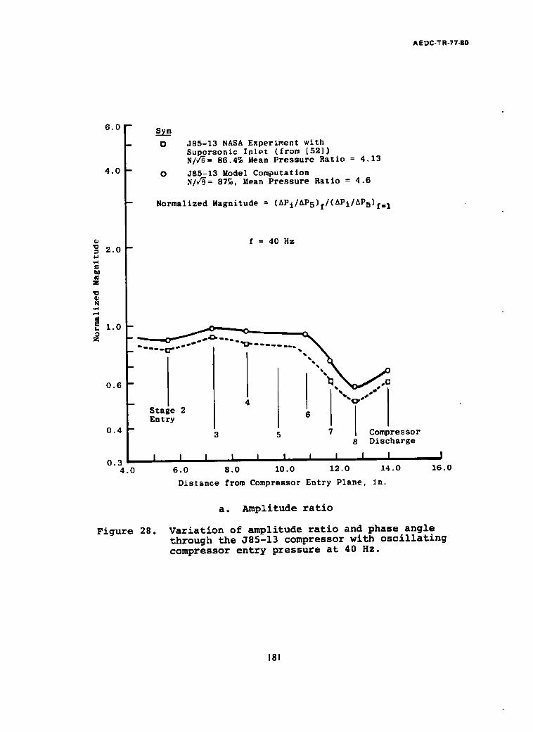
AEDC-T R-77-80
6 . 0
4 . 0
2 . 0
t
1 . 0 =o
0 . 6
0 . 4
0 . 3 4 . 0
D
Sym
D J 8 5 - 1 3 NASA E x p e r i m e n t w i t h S u p e r s o n i c I n l e t ( f r o m [ 5 2 ] ) N/,/SJ= 86.4% Mean P r e s s u r e R a t i o = 4 . 1 3
O J 8 5 - 1 3 Model C o m p u t a t i o n y/geeffi 87%, Mean P r e s s u r e R a t i o = 4 . 6
N o r m a l i z e d M a g n i t u d e = ( A P i / A P 5 ) f / ( A P i / A P 5 ) f f f i 1
f = 40 Hz
{ - - 4 I
S t a g e 2 61 i E n t r y [
- 3 5 7 C o m p r e s s o r 8 D i s c h a r g e
I I I I I I I I I I 6.0 8.0 10.0 12.0 14.0
D i s t a n c e f rom C o m p r e s s o r E n t r y P l a n e . i n .
I 16.0
a. Amplitude ratio
Figure 28. Variation of amplitude ratio and phase angle through the J85-13 compressor with oscillating compressor entry pressure at 40 Hz.
181
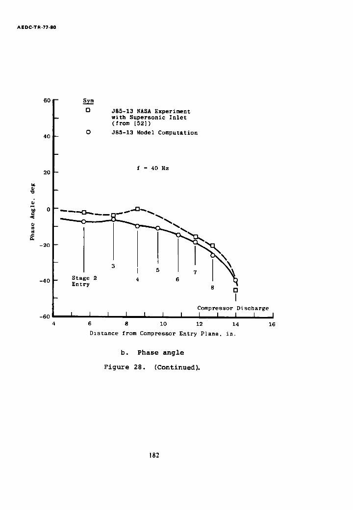
A E D C-T F1-77 -80
60 s~
C] J 8 5 - 1 3 NASA Exper iment w i t h S u p e r s o n i c I n l e t (from [52])
40 O J85-13 Model Computation
f = 4 0 Hz
"0
- 2 0
- 4 0 Stage 2 4 6 I Entry 8 [3
I Compressor lDischarge -eo I I I I I I I I I I I
4 6 8 I 0 12 14 16
D x s t a n c e f r o m C o m p r e s s o r E n t r y P l a n e , i n .
b. Phase angle
Figure 28. (Continued).
182
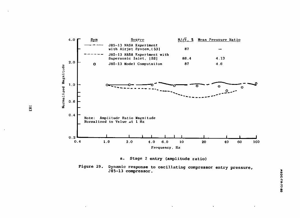
4.0 B Sym Mean Pressure Ratio
O0 t ~
2 . 0 - -
,P4
b~
1 . 0 --
t~ m
E 0 . 6 - -
0 Z
0 . 4 --
0 . 2 0 . 4
0
S o u r c e N L / 8 , %
J 8 5 - 1 3 NASA E x p e r i m e n t w i t h A i r j e t S y s t e m , { 5 3 ] 87
J 8 5 - 1 3 NASA E x p e r i m e n t w i t h S u p e r s o n i c I n l e t , L52] 8 6 . 4
J 8 5 - 1 3 Model C o m p u t a t i o n 87
4.13
4.6
•• ~ - ~ o o~. o- o o'-- "-Y "~- o o
-.-........._ o ...
N o t e : A m p l i t u d e R a t i o M a g n i t u d e N o r m a l i z e d t o V a l u e a t 1 H z
I I ,| I I I I I . I I I 1.0 2.0 4.0 6.0 10 20 40 60 100
Froquency, llz
Figure 29.
a. Stage 2 entry (amplitude ratio)
Dynamic response to oscillating compressor entry pressure, J85-13 compressor.
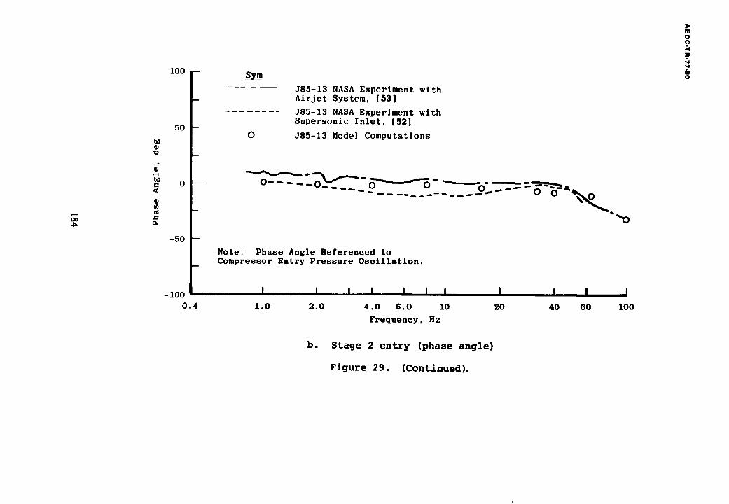
OO
v - 4
bD
®
e$
100
50 -
m
0 - -
m
- 5 0 - -
m
- 1 0 0
0 . 4
sym
O
J 8 5 - 1 3 NASA E x p e r i m e n t w i t h A i r j e t S y s t e m , [ 5 3 ]
J 8 5 - 1 3 NASA E x p e r i m e n t w i t h S u p e r s o n i c I n l e t , [ 5 2 ]
J 8 5 - 1 3 Model C o m p u t a t i o n s
N o t e : P h a s e A n g l e R e f e r e n c e d t o C o m p r e s s o r E n t r y P r e s s u r e O s c i l l a t i o n .
I I , , , I I I I I I I I J 1.0 2.0 4.0 6.0 10 20 40 60 100
F r e q u e n c y , i l z
b. Stage 2 entry (phase angle)
Figure 29. (Continued}.
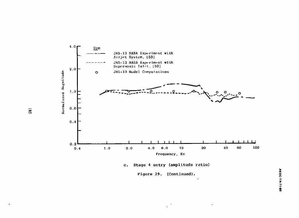
oo
4.a
"O
e.4
B L4 O
4 . 0
2 . 0
J
I . 0 B
i
B
m
0 . 6 - -
0 . 4 --
0 . 2
0 . 4
Sym
0
.J85-13 NASA Exp+,rim#.nt with Airj~t System. [53]
J85-13 NASA Exl)(.rim,~nt with Sup(,rsorlic Inl,.t. [52]
, I 8 5 - 1 3 M o d e l C ~ m q ) u t a t i o n s
~'~=':----2..--:"- o o ,o., - o ^ • =..P ,a~'% # f ~w ."
i , I I I I I I I I I I I I 1 . 0 2 . 0 4 . 0 6 . 0 10 20 4 0
F r e q u e n c y , Hz
I ~ i
60 100
Co Stage 4 entry (amplitude ratio)
Figure 29. (Continued). ill
0
-,i
w 0
Q
I
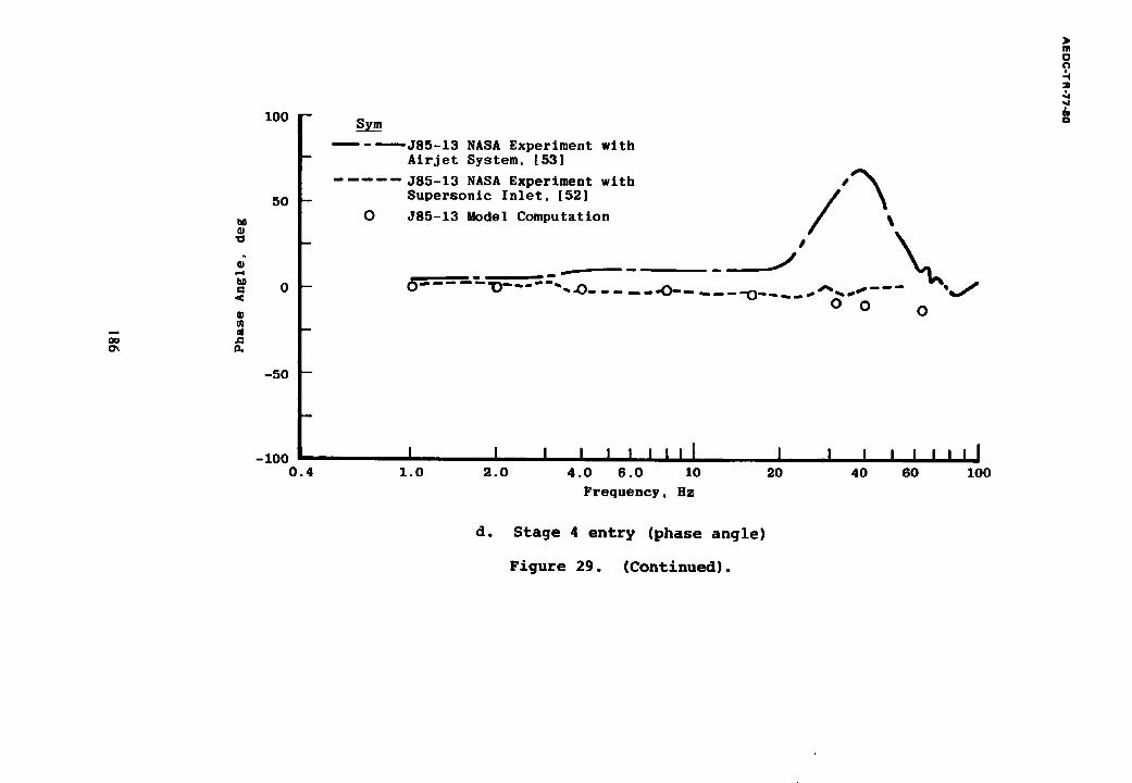
hO
t=.4 b~
a
O,
1 0 0 - -
5 0 - -
0 - -
- 5 0 - -
- 1 0 0 0 . 4
s ~ - - - - - ' - - J 8 5 - 1 3 NASA E x p e r i m e n t w i t h
A i r j e t S y s t e m , [ 5 3 ]
. . . . . J 8 5 - 1 3 NASA E x p e r i m e n t w i t h S u p e r s o n i c I n l e t . [ 5 2 ]
0 J85-13 M o d e l Computation / /s~ %
0 0 0
I I I I I I i I I J I I l i i n i i l I . 0 2 . 0 4 . 0 6 . 0 1 0 2 0 4 0 6 0 1 0 0
F r e q u e n c y . H z
m O
~J & o
d. Stage 4 entry (phase angle)
Figure 29. (Continued).
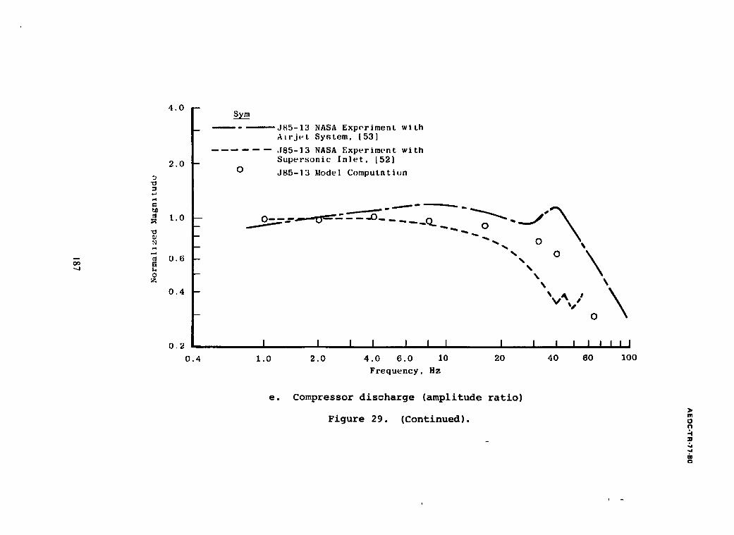
Oo
.1
"el
N
0 Z
4 . 0
2.0 m
1.0 -- m
m
0.6 --
0.4 --
0.2
0 . 4
Sym
0
J85-13 NASA Exporiment with Alrj,Jt System, [53]
.185-13 NASA Experiment with Supersonic Inlet, [52]
J85-13 Model Computation
. o \ %
%
X X \
V ~t \
0
I I I I I I I I I I I I ' i ' t 1.0 2 0 4.0 6.0 10 20 40 60 100
Frequency, Xz
e. Compressor discharge (amplitude ratio)
Figure 29, (Continued), m
? M
OB
o
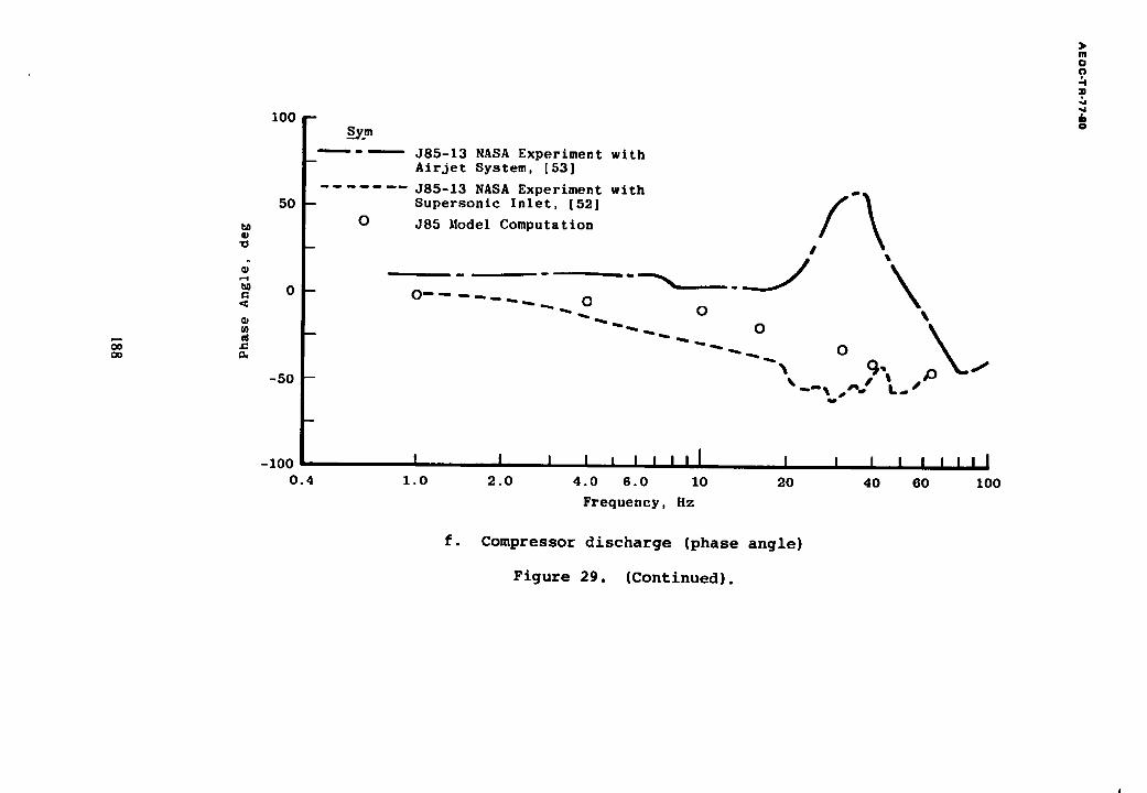
M
d 7. f:l
ffJ
1 0 0 -
50
-50
-100 0 .4
S_~vm "=------- J 8 5 - 1 3 NASA Experiment with
Airjet System, [53]
J85-13 NASA Experiment with S u p e r s o n i c I n l e t , [52] - - - - / ' /
0 J85 Model Computa t ion / I t
- - _ \
I 1 I I I I I III I I I I
1 .0 2 .0 4 . 0 6 . 0 10 20 40
F r e q u e n c y , Hz
I I I I I 6 0 1 0 0
f. Compressor discharge (phase angle)
Figure 29. (Continued}.
m o ? 3
& 0
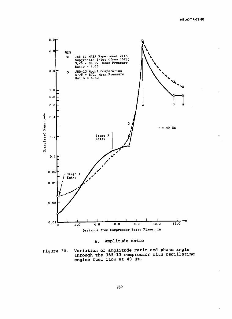
A E D C-T R -77-80
6 . 0 ,
4 . 0
2 . 0
1 . 0
0 . 8
0 . 6
0.4
m
s,
N 0 . 2
E
0 Z
0.1
0.06
0.04
s ~ [3
0
- S t a g e 1 E n t r y
J85-13 NASA Experlment wlth S u p E r s o n i c I n l e t ( f r o m 1 5 2 ] ) N/4~ = 8 8 . 2 ~ , Mean P r e s s u r e R a t l o = 4 . 6 3
J 8 5 - 1 3 Model C o m p u t a t l o n N/4~ = 87~ , Mean P r e s s u r e R a t l o = 4 . 6 0
S t a g e 2 E n t r y
J
I I 4 7 8
f = 40 HZ
0.02
0.01" 0
Figure 30.
2.0 4.0 6.0 8.0 I0.0
Distance from Compressor Entry Plane, in.
12.0
a. Amplitude ratio
Variation of amplitude ratio and phase angle through the J85-13 compressor with oscillating engine fuel flow at 40 Hz.
189

AEDC.TR-77-80
6 0 -
s,m - - - 0 - - J 8 5 NASA E x p e r i m e n t w i t h
S u p e r s o n i c I n l e t , 152]
40 - --0-- J85-13 Model CompuSatlon
20 - f = 40 Nz
_2o t •40
l I I -60 0 2.0
S t a g e 1 E n t r y
I l I I I ] I I J I 4.0 6.0 8.0 10.0 12.0
D x s t a n c e f r o m C o m p r e s s o r E n t r y P l a n e , i n .
b. Phase angle
Figure 30. (Continued).
190
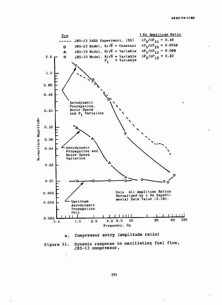
AE DC-T R-77-80
¢., ,o
4.1 . -4 ¢
¢ b;
.,..,
E L
c.
2 . 0
1 . 0
0 . 6 0
0 . 4 0
0.20
0. i0
0.06
0.04
0 . 0 2
0.01
0. 006
0.004
0.002 " 0 . 4
s_~ J85-13 NASA Experiment, [52]
O J85-13 Model, N/~ = Constant J 8 5 - 1 3 M o d e l , N / ~ = V a r i a b l e
D J85-13 Model. N//'O = Variable
~0
%,
P l = V a r l a b l e
1Hz A m p l i t u d e Ratio
&P5/AP13 = 0.16 AP5/AP13 = 0.0016 AP5/AP13 = 0.098 AP5/AP13 = 0.23
Aerodynamlc \ ~ Propagation, Rotor Speed and Pl Variation
"n \,,
aml c ~ • Propagation and~ ~ ' Rotor Speed ~ ~ Varlation ~ Z ~ ~ ~
0/0 Note All.Amplitude Ratios Normalized by 1 Hz Experi-
ZUpstream mental Data Value (0.16). Aerodynamlc Propagation Only i I I I I I l i l l l I l I ' l l l ] l 1.0 2.0 4.0 6.0 I0 20 60 lU0
Frequency, Rz
Re
Figure 31.
Compressor entry (amplitude ratio)
Dynamic response to oscillating fuel flow, J85-13 compressor.
191
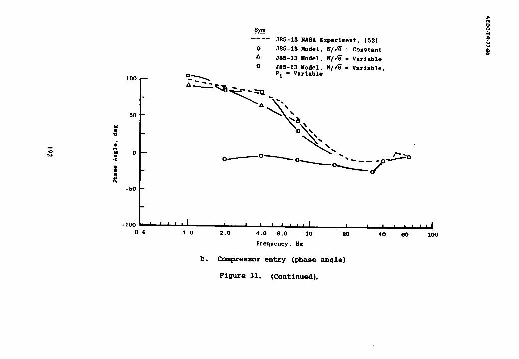
m
~J
~q
m J:
100 --
50 -
0 --
D
-50 -
B
- 1 0 0 0 . 4
Sym
. . . . J 8 5 - 1 3 NASA Exper im ent , [52]
0 J 8 5 - 1 3 Model. N / , ~ = C o n s t a n t
A J 8 5 - 1 3 Model, N / ~ = V a r i a b l e
t:] J 8 5 - 1 3 X o d e l . N / / 8 = V a r i a b l e . " _ ~ Pl = V a r i a b l e
! i i I I i
1 . 0
b.
I I i n | | I I i i
2 . 0 4 . 0 6 . 0 tO 20
Frequency , Hz
Compressor entry (phase angle)
i I
4O
I I ! I m |
6 0 1 0 0
m
O n :m
~J
& o
Figure 31. (Continued).
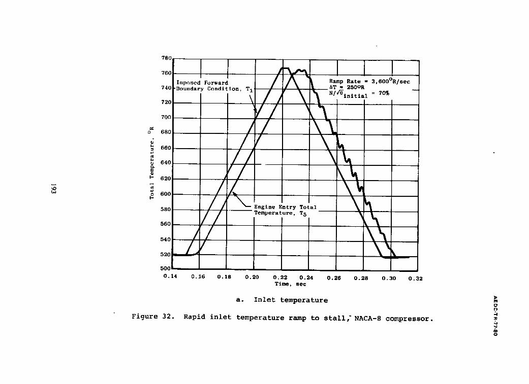
~o
780
760
740
720
700
o 680
d = 660 , J
o 640 E
~" 69-0
o 600
580
560
540
50( 0 . 1 4
Figure 32.
I m p o s e d F o r w a r d B o u n d a r y C o n d i t i o n
/ / /
/ /
, T 1
\
/ / /
/ ~ ' L R.p Rate = A T = 250oR
/ / <i'r61 n i t i al 1
II ' i
E n g i n e E n t r y T o t a l T e m p e r a t u r e , T 5
! 3,600°R/sec
= 7 0 %
I
P~I IL~
O. 16 O. 18 0.20 0.22 0.24 0.26 0.28 0.30 0.32 Time, see
a. Inlet temperature
Rapid inlet temperature ramp to stall," NACA-8 compressor.
> m
o
& O
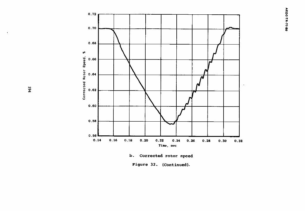
~D 4~
0.72
0.70
0.68
• o 0 . 6 6 oj
f., 0 . ~ 0 . 6 4 0
oj 4 J u w 0 . 6 2 k 1.4 0
¢J
O. 60
O. 58
\ / \ / \
/
!
> m O
9
R O
0.56
O. 14 O. 1 6 0 . 1 8 0 . 2 0 0 . 2 2 0 . 2 4 0 . 2 6 0 . 2 8 0 . 3 0 0 . 3 2
T i m e , s e c
b. Corrected rotor speed
Figure 32. (Continued}.
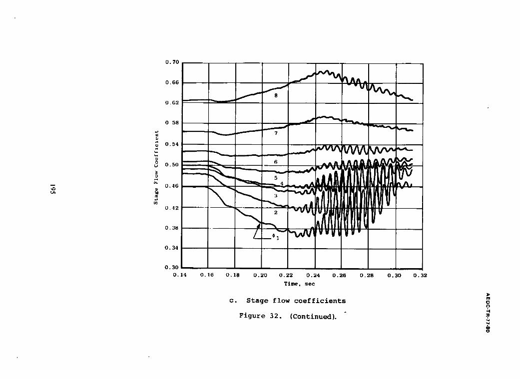
m ~D t~
O. 70
000
0 58 ~ ~ I =--, ~ n ~ " t , , - -
o.,t2 ~ rV b/ m tl V '
0.38 ~ ' ~ A ,
0.34
O. 30
0 . 1 4 0 . 1 6 0 . 1 8 0 . 2 0 0 . 2 2 0 . 2 4 0 . 2 6 0 . 2 8 0 . 3 0 0 . 3 2
Time, sec
Co Stage flow coefficients
Figure 32. (Continued).
m
m o
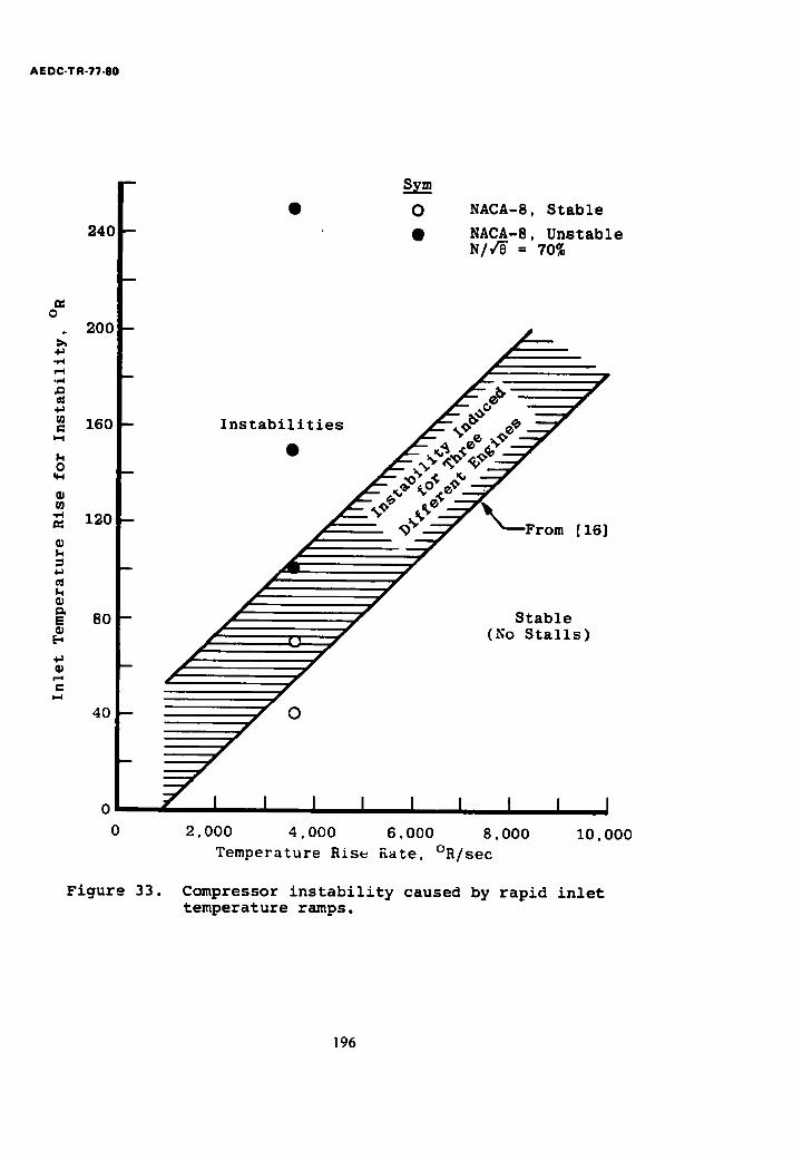
AE 0C-TR-77-80
240
O
200
°p4
4J
160
O
"~ 120
E 80
t,-
40
O
I n s t a b i l i t i e s
NACA-8, S t a b l e
NACA-8, Unstable
N / / 0 = 70%
0
~"~ ~-=-From [16]
S t a b l e (No S t a l l s )
0 L
0
Figure 33.
2 , 0 0 0 4 , 0 0 0 6 . 0 0 0 8 . 0 0 0 T e m p e r a t u r e Ris~ R a t e , °R/sec
1 0 , 0 0 0
Compressor instability caused by rapid inlet temperature ramps.
196
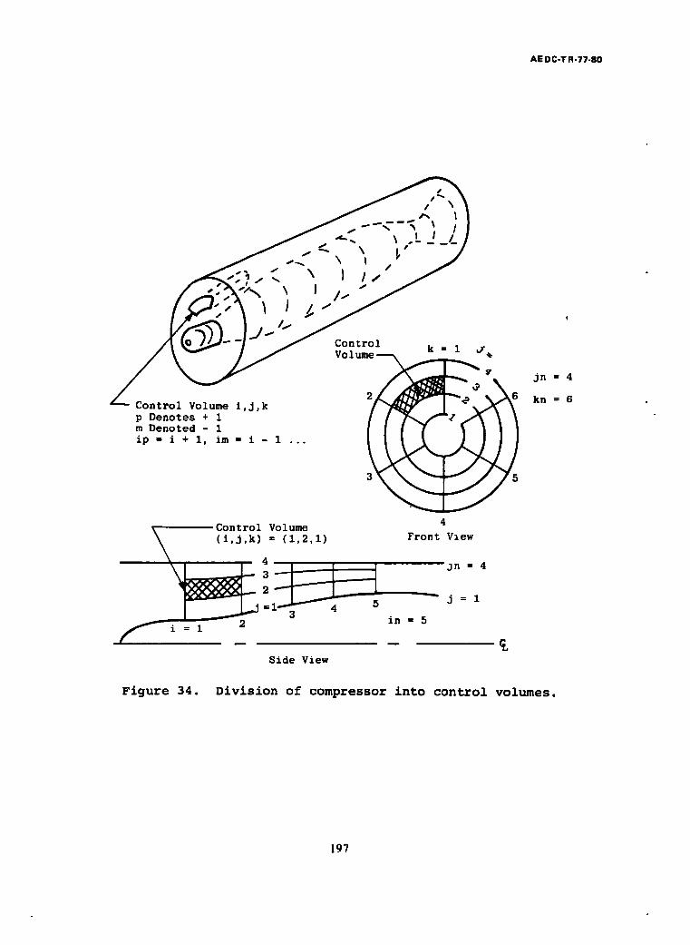
AE DC-T R-77-80
o , \ . Control Volume i , j , k I ~ I " ~ \ p Denotes + i / [ ~/~"? /~ ~ m D e n o t e d - 1 I I ! l ~ | I I ip = i + I, im = i - 1 ... ~ k ~ / ]
4 Control Volume (i,j,k) - (1,2.1) Front Vxew
i = 1 2
Side View
"jn=4
j -- 1
in = 5
%
i n - - 4
kn =6
Figure 34. Division of compressor into control volumes.
197
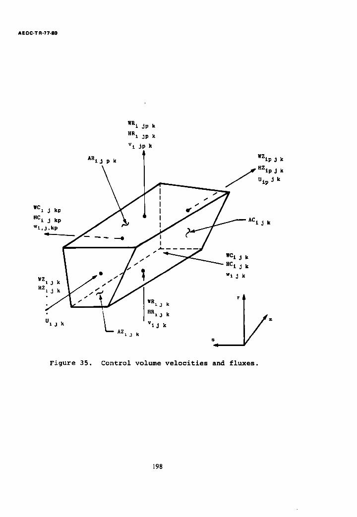
AEDC-T R-77-80
WC ,z j kp HCi j kp w i , j , k p
wz t j k HZ x j k
U xJ k
ARt J p k
• /
J -
WRi jp k
HRx jp k
v i Jp k
S ,
J
; /
y IWRIj k
L HRx3 k
v i i k AZ xj k
J
J
f
WZip J k
HZip J k
Uip j k
ACij k
wci j k
HCl J k
W i j k
r
Figure 35. Control volume velocities and fluxes.
198
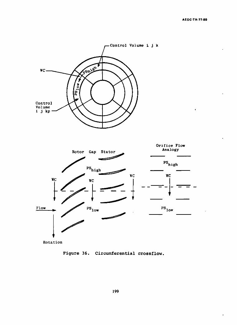
AEDC-TR-77-80
Volume i j k
WC
Cont Volume / ~X ~ I / ~ / / i j kp ~
Flow
R o t o r Gap S t a t o r
/ P S h i g ~ .ic
/
Orifice Flow Analogy
m m
PShig h
WC
PSIo w
Ro t a t ion
Figure 36. Circumferential crossflow.
199
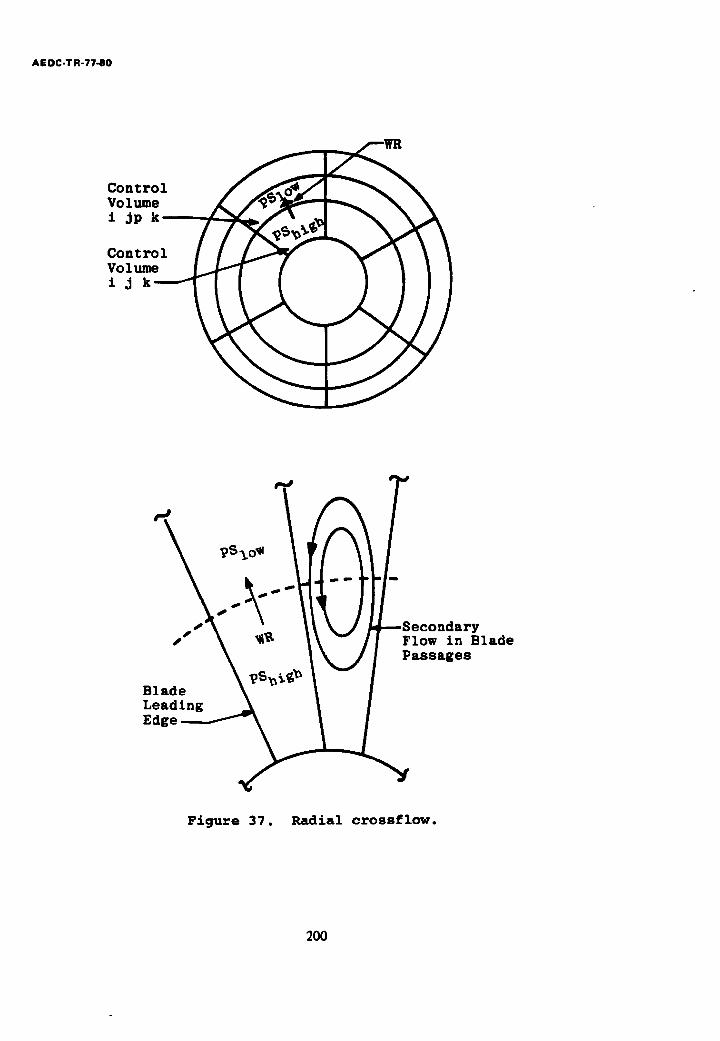
AE DC-T R-77-80
C o n t r Volum i 3P
C o n t r Volum i j k
Blade Lead ing Edge
, ~ e c o n a a r y F l o w i n B l a d e Passages
w
Figure 37, Radial crossflow.
200
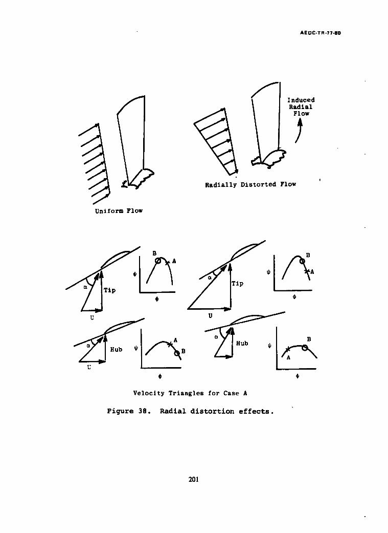
AE 0C-TR-77-80
I n d u c e d R a d i a l
F low
R a d l a l l y DI ow
U n i f o r m F l o w
U 0 *
V e l o c l t y T r i a n g l e s f o r C a s e A
Figure 38. Radial distortion effects.
201
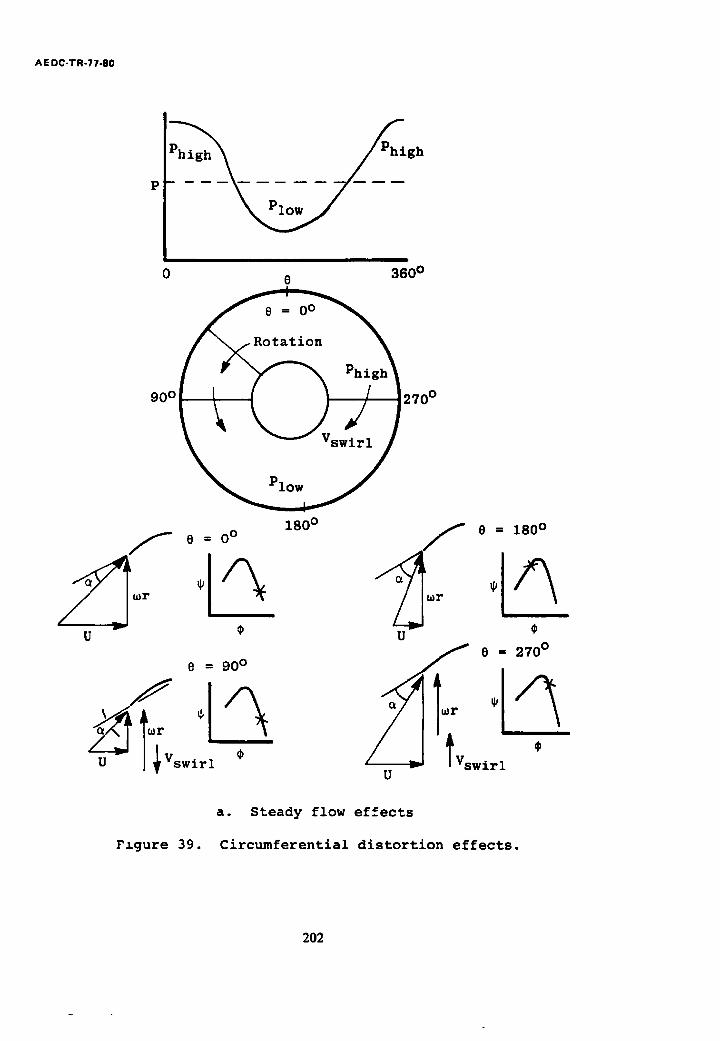
AE DC-TR-77-80
p
0 0 3600
90 ° 270 °
f 0 iO °
U $
e = 90 °
f
U | ~ Vswirl
180 ° e i IS0£ U $ e]27o
Z J IVswirl ° U
a. Steady flow effects
F~gure 39. Circumferential distortion effects.
202

AEDC-TR-77-80
270 . . . .
9 0 ~ . / / / P l:ov,' " " ,%_ / P
I
~"'- ~ dy.
0 360 5, deg
0 360 0, deg
~dyn
b. Unsteady flow effects
Figure 39. (Continued).
203

AE DC-T R-77-80
C~
/ i | ~ C i s t a l l
' f
V C d~ re f
Angle of Attack, a
m = 40 1.0-- -- / m= 20
. ~ . g e of Exper l - / ~ -<> - I / " _ m e n t a l Data, ~ ~ , ~ ~
08 t361 --~ /~.~\ h-'l
o 0 0.01 0.02 0.03 0.04 0.05
C ~a Vre f %t ' r ad lans
c. Unsteady stall effects
Figure 39. (Continued).
204
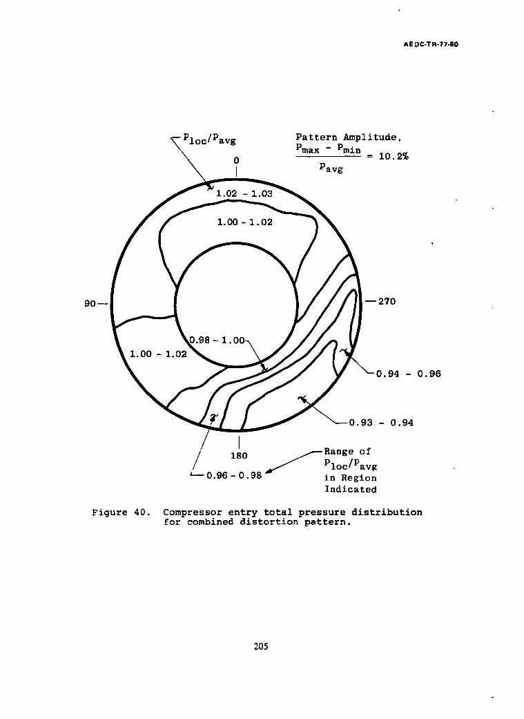
AE DC-T R-77-80
Ploc/Pavg Pattern Amplitude, Pmax - Pmin
= lO.2% Pavg
1.00 - 1.02
90-- -- 270
1.00 - 1.02
- 1
9 4 - 0 . 9 6
Figure 40.
0 . 9 3 - 0 . 9 4
/ i / 180 s Range of
Ploc/Pavg 0.96-0.98 in Region
Indicated
Compressor entry total pressure distribution for combined distortion pattern.
205
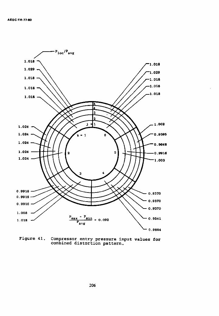
AEDC-TR-?7.80
' ~ P l o c / P a v g
1.018 "--~
1. 029 - - ~
1. 018 -.-.
1 .018
1.018
.018
.029
.018
018
1. 024
1. 024
1 .024
1.024
1.024
k = l
2
1 .002
0.9595
3 4
0 . 9 9 1 6
O. 9916
O. 9916
1 . 0 0 8
1 . 0 1 8
Figure 41.
0 . 9 3 7 0
0 . 9 3 7 0
0 . 9 3 7 0
Pmax - Pmin = 0.092 ~ ~ - ' - 0 . 9 5 4 1 P a v g
0.9884
Compressor entry pressure input values for combined distortion pattern.
206
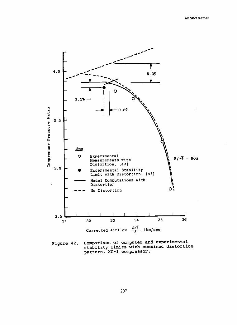
A E DC-T R-77-80
O --d 4~
O
k C
E O
4.0
3.5
3.0
2.5 31
1.3% ~
~S ~,,a~ ~ ~
f 5.3%
O. 8%
Sym
O Experimental Measurements with Distortion, [43]
Experzmental Stability Limit with Distortion. [43]
Model Computations with Distortion
No Distortion
i I I I I 1 32 33 34
Corrected A i r f l o w - - = - - ibm/sec
o',
I = • 35 36
~ / , ~ = 9 0 %
Figure 42. Comparison of computed and experimental stability limits with combined distortion pattern, XC-I compressor.
207
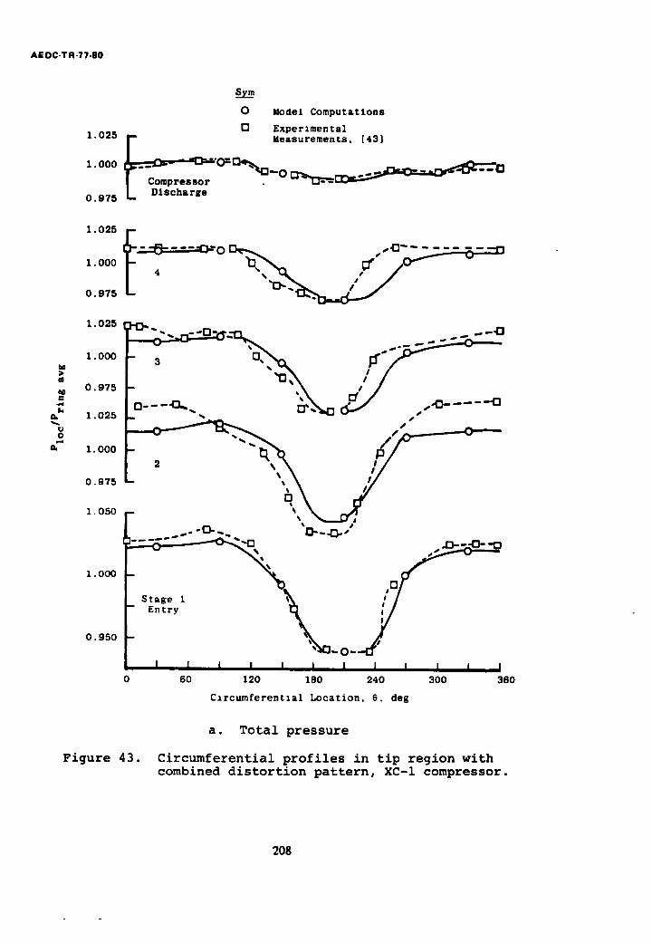
AE DC-TR-77-80
0 Model C o m p u t a t i o n s
0 Expe rzmen ta l 1 .025 F Measurements , [43]
!
0 . 9 7 5 L D i s c h a r g e
L
o
i .025
1. 000
0 .975
1 .025
1. 000
I 0.975
1.025
1. 000
0.975
I. 050
1. 000
O. 950
Figure 43.
~ " 4-~ ====~>'0~ "'~-- G "FI
- ' , , , ' 7 - - ~,N .~./ .<>- .... o---~-.. ~'-~o 6~ ..'~--- "
-
- " ~ - o--.d' ' I I I I I I I I I I I
0 60 120 180 240 300 360
C i r c u m f e r e n t i a l Location, 6. deg
a. Total pressure
Circumferential profiles in tip region with combined distortion pattern, XC-I compressor.
208
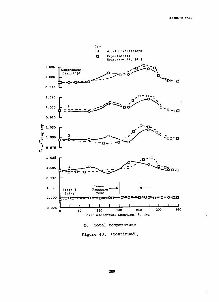
AE DC-T R-77-80
1 . 0 2 5
1. 000
0 . 9 7 5
1.025
1. 000
0.975
:) 1.025 a
bo
1. 000
u
o 0. 975
1. 025
1. 000
0.975
1 . 0 2 5
1. 000
0 . 9 7 5
s_~ O Model C o m p u t a t I o n s
[3 E x p e r i m e n t a l M e a s u r e m e n t s , [43]
/ Discharge / O " ~ " ' 0 ~" 6 I " - - 6
/ D - D ~ o
o o - - d... ~ ' ~ "o -cu
.0"-- -0. "
. . . . [] _ . -'0 ~"'01 ":OO" []
- / O . O " -O, ',
_ 2 ~ O ~ _ _~/. D ~ O ~ ~ 1 3 . D "--:8--o- - -
- - S t a g e 1 P r e s s u r e ~ E n t r y Zone
----~0 . . . . 0 =--~D - - ~ O D - ' ~ D ' = O ---~- D ---D O=D =~D---O--D:D
l I I I i I I I I I i • 0 60 120 180 240 300 360
C i r c u m f e r e n t i a l L o c a t i o n , O, d e g
b. Total temperature
Figure 43. (Continued).
2 0 9
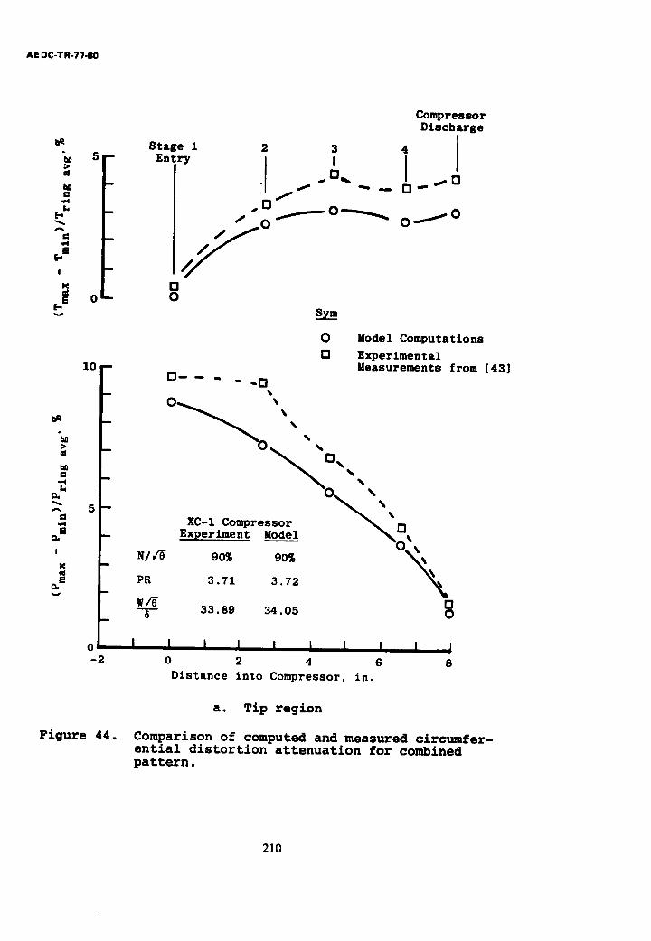
AE DC-TR-77-80
~a "w 5- I
!
K
[] 0 -
10--
m
= m
[]
!
M
E
n
0 -2
Compressor
Discha rge
Stage 1 i !
,, m ~ ..0~ ~ --
/~O ~ O ~ O ~ o
O O
O - - _ .
O O
Model Computa t ions E x p e r i m e n t a l Measurements from [43]
" -0 O ~ •
~ o q ~ ~ • XC-i Compressor ~ ~]
Experiment Mode___1 ~ %
PR 3.71 3.72
3 3 . 8 9 3 4 . 0 5
I I I I i I # I I 0 2 4 6 8 Distance into Compressor, in.
a. Tip region
Figure 44. Comparison of computed and measured circumfer- ential distortion attenuation for combined pattern.
210
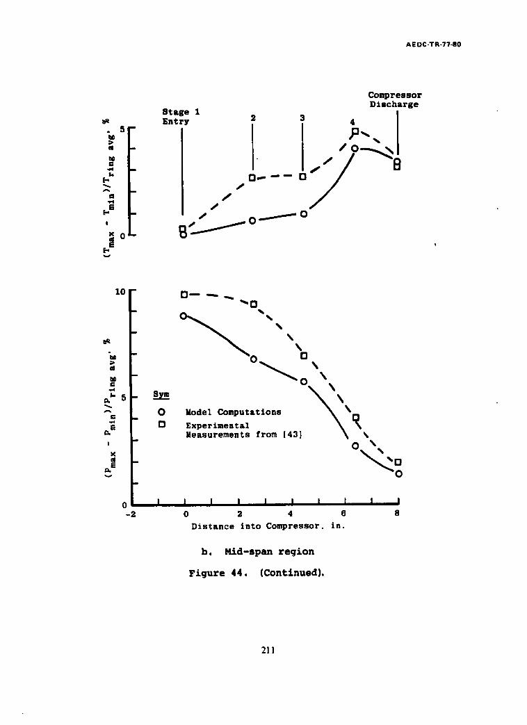
AE D C - T R - 7 7 - 8 0
C o m p r e s s o r D i s c h a r g e
S t a g e I E n t r y 3
. 5
/ O" ---- O /
j ,a
o ==
10
B
"u -
B
"" O ~ D
!
a _ N
0 ! - 2
r i m
%%%%
Model C o m p u t a t i o n s
E x p e r i m e n t a l Me a sur e ment s from 1 4 3 ] %%
0 ,,
! I I I I l I I i 0 9. 4 6 8
Distance in to CompreBsor. in.
b . Mid-span region
Figure 44. (Continued).
211
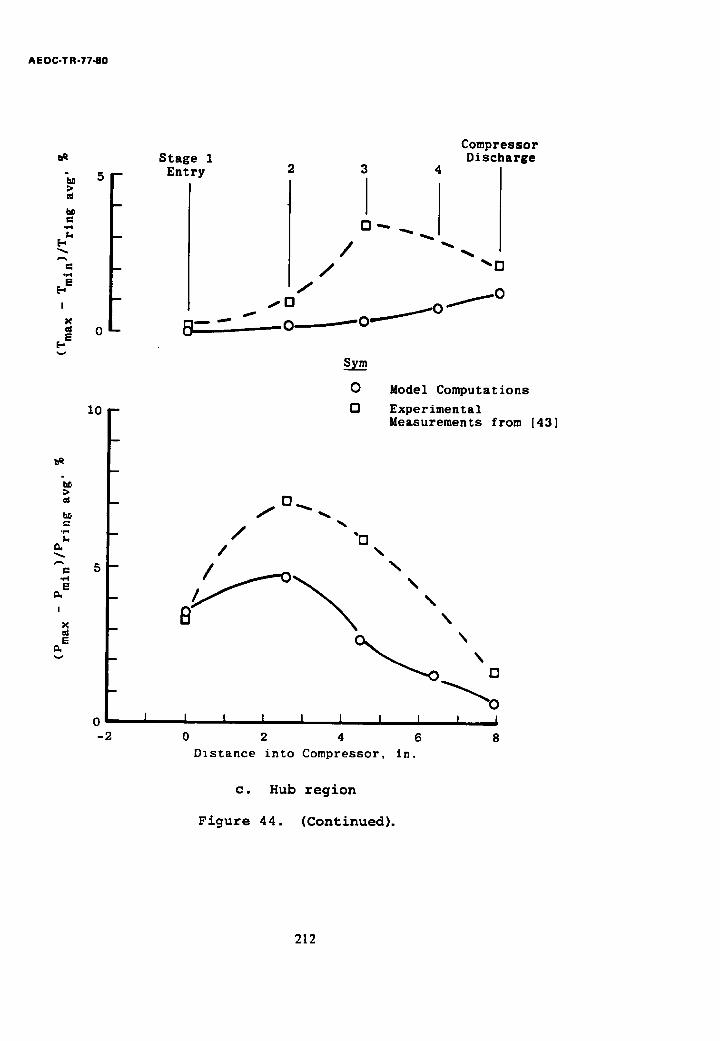
AEDC-TR-7740
!
E E-
e-
. p 4
E
I
X
E
5 i
m
i
i
i
0 -
1 0 -
m
m
n
m
5 - -
m
n
0 - 2
Stage 1 E n t r y
s
/
- - 0
/ /
3 4
Compressor D i s c h a r g e
"[3
/ o
_o
sym
O
D
Model Computations
Experimental Measurements from [43]
o
/ -Q /
\ \ \
\\
l l I I I i I I J
0 2 4 6 8 D;stance into Compressor, in.
c. Hub region
Figure 44. (Continued).
212
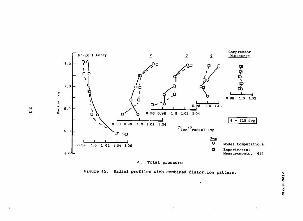
t~
8 . 0
7.0
"4
6 . o t~
5.0
m
4.0 m
_ Compressor St.',1~_e 1 hntry 2 _3 4_ Discharge
- ~',I /3 ? " ° " ' , /, \
O D I 0.98 1.0 1.02
0 , 9 8 1 . 0 1 , 0 2 I l I
• / 0 O. . 1 .0 1.02 1.04
I I I [0= 210 deg] 1.0 1.02 1.04
Ploc/Pradial avg
[] 0 \ ~ t I .96 0.98
L , I I I Sym
o . 9 8 t.O 1 . 0 2 1.04 *.06 0 rn
Model Computations
ExperLmental Measurements, [43]
a. Total pressure
Figure 45. Radial profiles with combined distortion pattern. m 0
9 -4 =m
"4
0
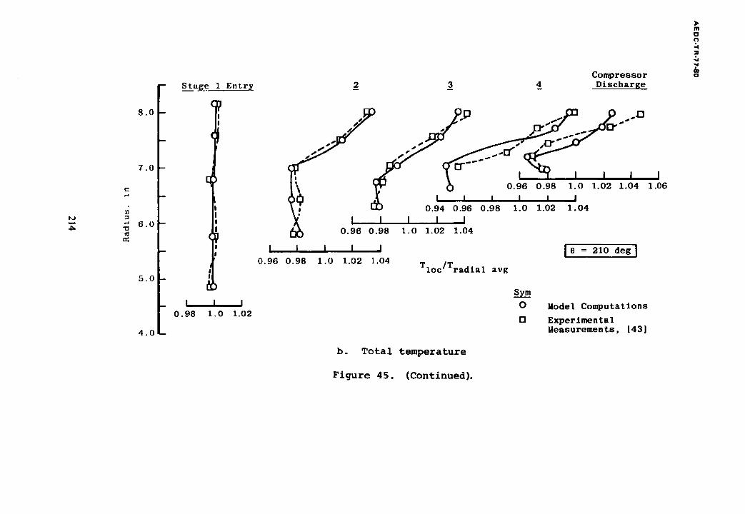
m
4~
8.0
7.0
6.0
5.0
4.0
S.....~ta.~e 1 Entry
c~
I i I 0.98 1.0 1.02
Compressor 2 3 4 Dischar6e _ _ w
j o o., ,o.o. A I I I I I I
0 .94 0 .96 0 . 9 8 1 .0 1 .02 1 . 0 4
I I l I I 0 . 9 6 0 . 9 8 1 . 0 1 .02 1 .04
[ I I ] J [ 6 = 210 d e g ] 0.96 0.98 1 0 1.02 1.04
" T l o c / T r a d i a l a v g
sym
0
0
M o d e l C o m p u t a t i o n s
Experimental Measurements, [43]
b. Total temperature
m
n
3
& o
Figure 45. (Continued).
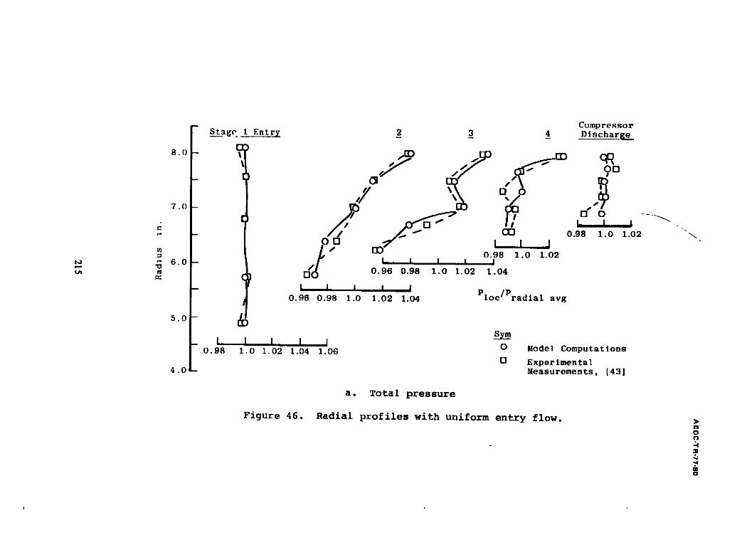
10
8 . 0
7 . 0
-s
" 6 0 --
5.0 -
w
4.0 -
St~go 1 Entry
o Compressor
2 3 4 D i scha rge
t tD ~ ~ ED C~_ L
,I ",;
/ / ./~- ~" CO 0.98 1 . 0 1 .02
L [D 0 . 9 8 1 . 0 1 .02 r • i i i i
d~ 0.96 0.98 1.0 1.02 1.04
L I I I I 0.96 0.98 1.0 1.09. 1.04 PloclPradial avg
L I I I I 0 . 9 8 1 , 0 1 .02 1.04 1 .06
s~m
O
B Model Computa t ions
E x p e r i m e n t a l Measurements , {43]
a. Total pressure
Figure 46. Radial profiles with uniform entry flow. m
O O
& o
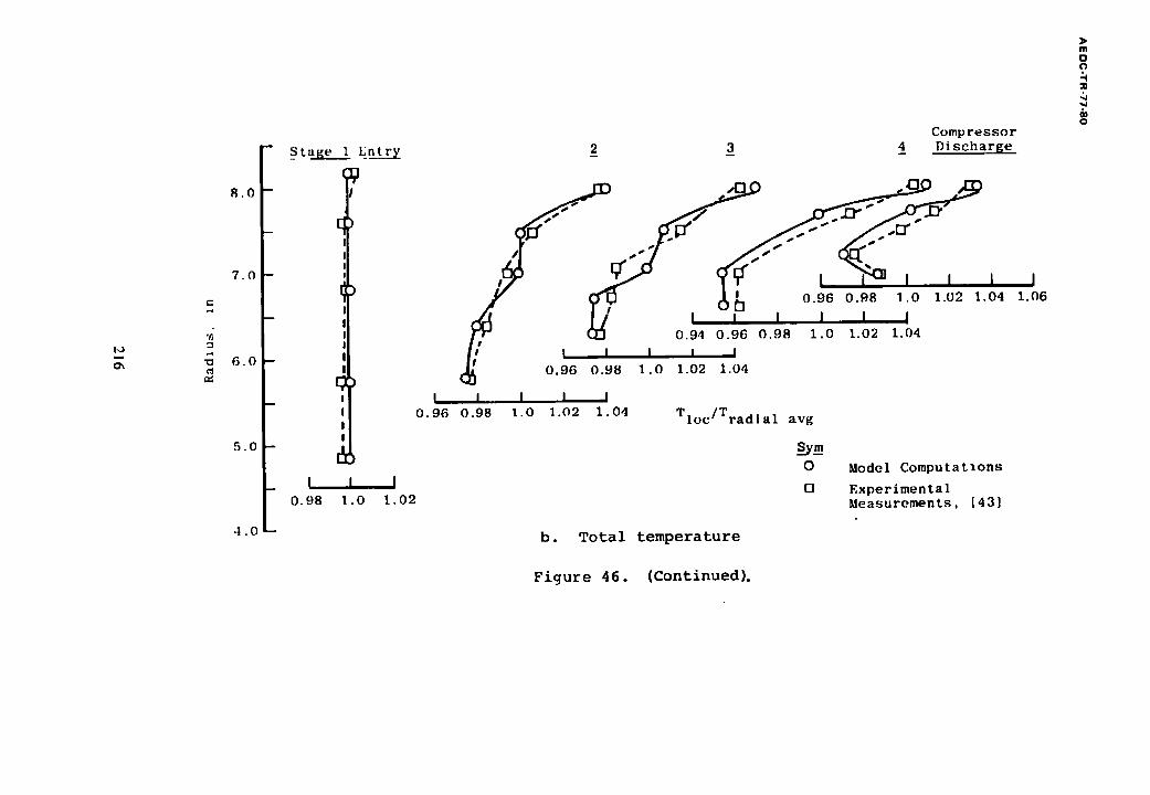
t , o
R . O -
7 . 0 -
c-,
,=4
, / )
6 . o - c~
m
5 . 0 -
m
• ! . 0 - -
s'ta e_~_/ L.nt~
I
)
I I I I I I
)
I I I 0 . 9 8 1 . 0 1 . 0 2
Compressor 2 3 4 D i s c h a r g e
6 Y , , ~ 6~ 0 . 9 6 0 . 9 8 1 . 0 1.02 1 .04
Ii , - F i , , J ,/V" m 0.94 0.96 0 .98 1.0 1.02 1.04 I,* I i I ' J
( ~ 0 . 9 6 0 . 9 8 1 . 0 1.02 1.04
I I I , ' •
0 . 9 6 0 . 9 8 1 .0 1 .02 1 . 0 4 T l o c / T r a d i a l a v g
s_ym
0
El
Model Computatlons
Experimental Measurements, [43]
b. Total temperature
I 1 . 0 6
m
O f~
m O
Figure 46. (Continued).
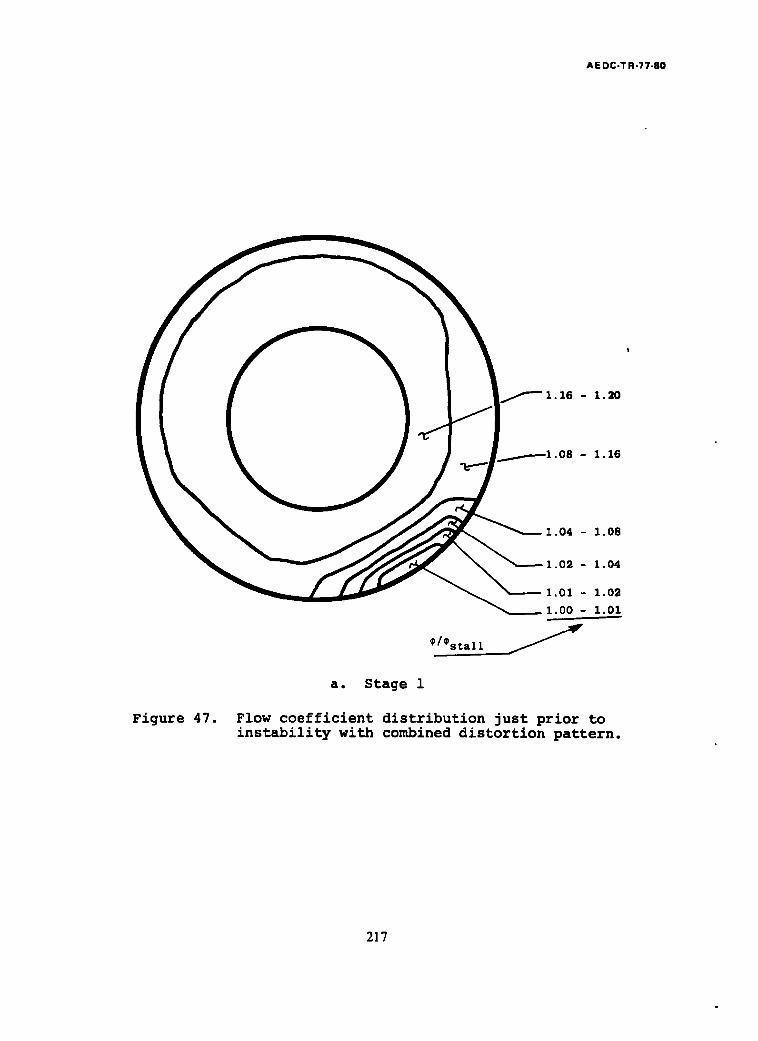
AEDC-TR-77-80
Figure 47.
\ !
~ 1 . 1 6 - 1.20
. . t . . . ~ l ~ l . 08 1.16
O I
~ 1 . 0 4 1.08 1
~ ~ 1 . o 2 - 1 . o 4
1.01 - 1.02 1.00 - 1.01
~/~stall S
a. Stage 1
Flow coefficient distribution just prior to instability with combined distortion pattern.
217
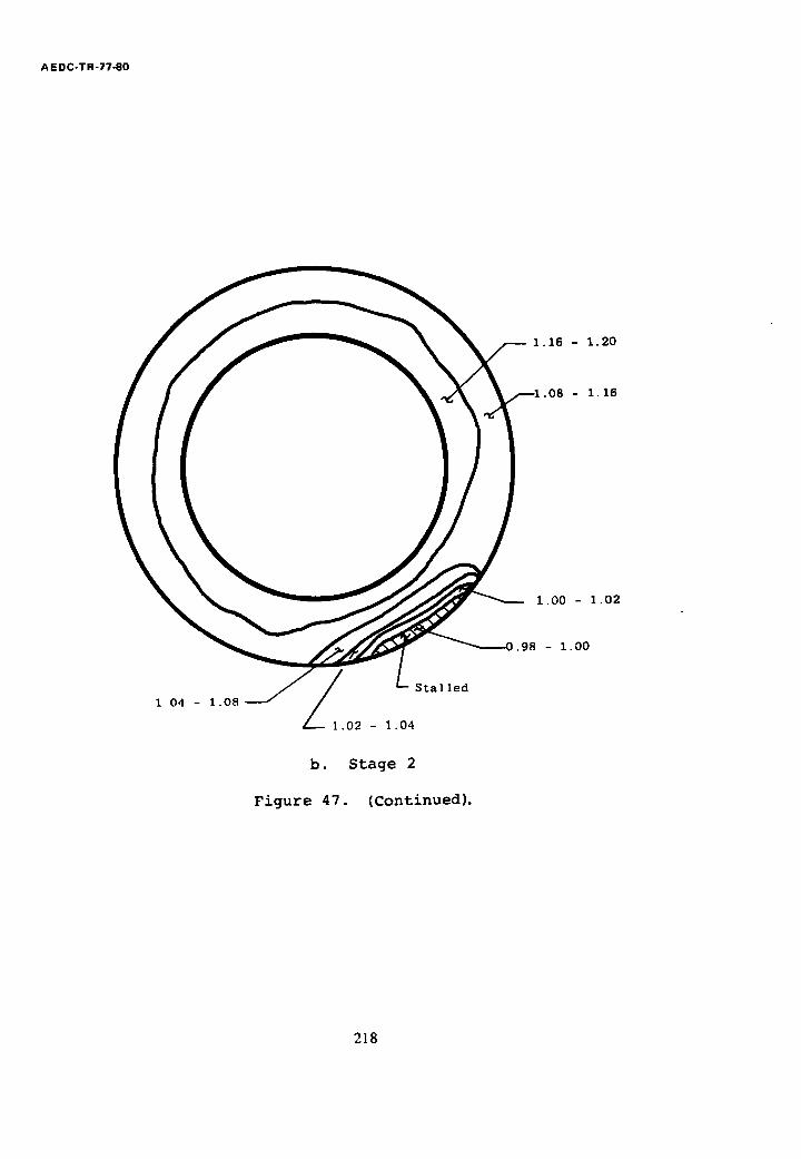
A EDC-TR-77-80
1.16 - 1.20
.08 - 1.16
1.00 - 1.02
1 04 - 1.08
/ / L S t a l l e d
1 . 0 2 - 1 . 0 4
b. Stage 2
Figure 47. (Continued).
. 98 - 1.00
218
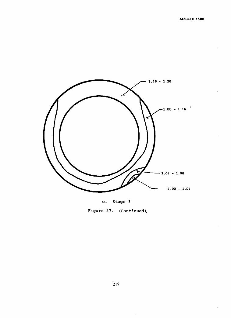
AEDC-TR-77-80
--- 1.16 - 1.20
!
f 1.08 - 1.16
1.04 - 1.08
1.02 - 1.04
c. Stage 3
Figure 47. (Continued).
219

AE DC-TR-77-80
1.04 - 1.08
- 1.04
1.00 - 1.02
- - 0 . 9 8 - 1.00
S t a l l e d
0.94 - 0.98
d. Stage 4
Figure 47. (Continued).
220
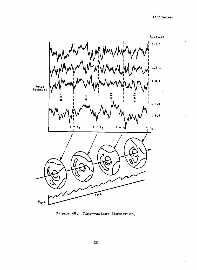
AEDC-TR-77-80
Location
Total Pressure n I m
R
l n
-- I =
l I I,i,I
V v 1 r v '1
I ~ ~ ~ ~ I ii2,1 [ ~ l 1 , 3 , 1
m m [
_ I _ I
: I : I
l l ~ l i,j,k I 1 , 6 , 5
t = t 1 t --. t 2 t = t 3 t -- t 4
I / I I i
/,
Figure 48. Time-variant distortion.
221
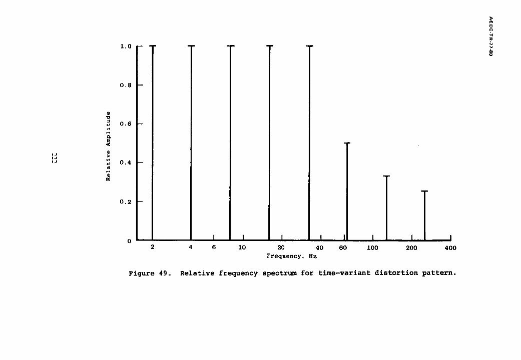
I J I J I - )
0) >
,F4
r ~
1 . 0
0 . 8
0 . 6
0 . 4
0 . 2
0 2 4 6 10 20 4 0 6 0 100 2 0 0 4 0 0
F r e q u e n c y , Hz
n
co o
Figure 49. Relative frequency spectrum for time-variant distortion pattern.
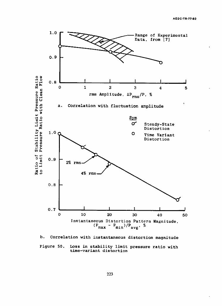
AEDC-TR-77-80
1.0 F ~ ~Range of Experimental
0 . 9 ~ [71
O~ "~0 ~ o.8 I I I I I
0 1 2 3 4 5 G
~ rms Amplitude, AP /P, % m ~ rms
= a. Correlation with fluctuation amplitude
• ~o ~ .r'4 4-) ~ 0 4 Steady-State
Dis tor t ion ~ l o O Time Variant . ,~
= I__ ~ Distor t ion
c a ~
~. . 4 J
o . 9 - v~ 2% r m s ~
0 0 . 8 -- 4% rms--/
0.7 I I I I I 10 20 30 40 50
Instantaneous Distortion Pattern Magnitude, (Pmax - Pmin)/Pavg' %
b. Correlation with instantaneous distortion magnitude
Figure 50. Loss in stability limit pressure ratio with time-variant distortion
223
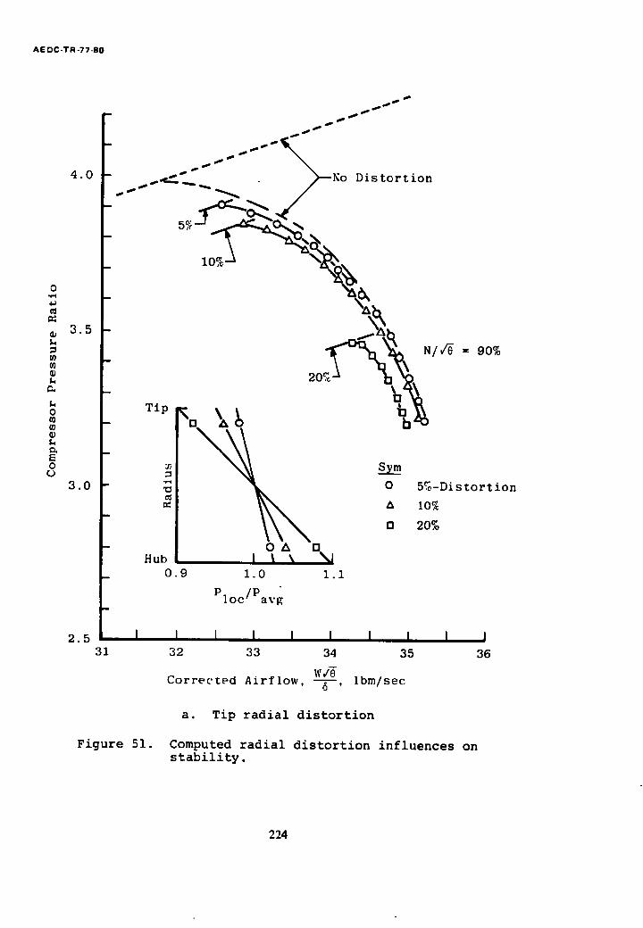
AE D C-T F1-77-80
4 . 0
2
3 . 5
¢ .
O
&9
t~ E O
3 . 0
2.5
,jpS
- ' " ")---No .. ~ 4~. _. . ~ Distortion
I0,~ %
-
N / ~ = 90% 20.~
T i p
e~ ee
1 . 0
l o c / P a v g
O 5%-Distortion
10~
U 20.%
O A tl I I \ \ J
1 . ! Hub
0 . 9
i I I I I I I I I I 31 32 33 34 35 36
C o r r e c t e d A i r f l o w , 6 ' I b m / s e c
a. Tip radial distortion
Figure 51. Computed radial distortion influences on stability.
224
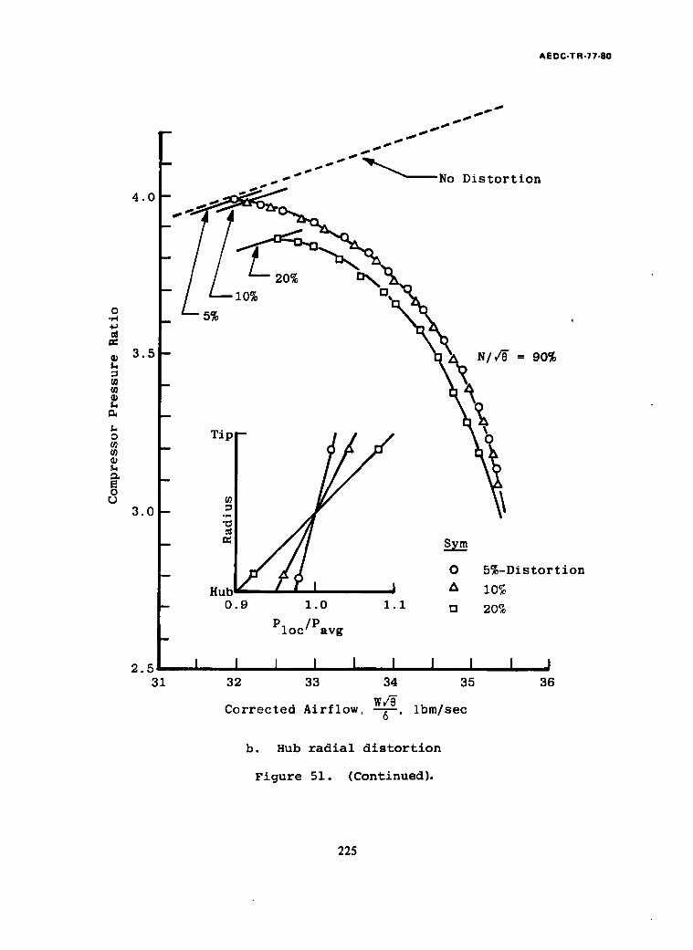
AEDC-T R-77-80
0
O
E O
-- " " D i s t o r t ion
4 . 0 _ ~ ~
3,5 - -
m
3.0 -
m
2.5 31
5%
10% 2o~ ~ ,
N / ~ = 9 0 %
Tip
Hub 0 . 9 1 .0 i . I
P l o c / P a v g
i i I [ I 32 33 34
Corrected Airflow, 6 '
O 5%-Distortion
n 1o%
D 20,~,
I I I I 35 36
I b m / s e c
b. Hub radial distortion
Figure 51. (Continued).
225
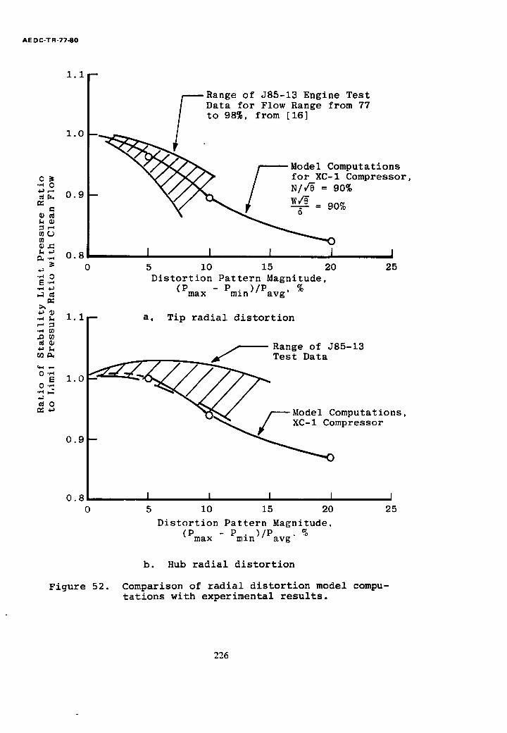
AE DC-TR-77-80
1.1
1.0
s Range of J85-13 Engine Test Data for Flow Range from 77 to 98%, from [16]
y Model Computa t ions f o r XC-1 Compressor , N / ~ = 9 0 % w_q =
I I I I I 5 10 15 20 25
D i s t o r t i o n P a t t e r n Magni tude ,
• ,..4 C 4 J r = . er.,., 0 . 9 - - 1
tw :3, '~
¢~,,.C t . . ,~ ~, .,, 0.8
• ,-.I 0
'~ ~ ( Pmax Pmin)/Pavg, %
~ 1.11-- a, Tip radial distortion
1 ~ | ~ Range of J85-13 ~ I ~ s" Tes t Data
~o ~ ~ /---- Model Computations,
0.9 _ ~,~ _/ XC-I C o m p r e s s o r
0 . 8 I I I I I 0 5 I0 15 20 25
Distortion Pattern Magnitude, (Pmax - Pmin) /Pavg" %
b. Hub radial distortion
Figure 52. Comparison of radial distortion model compu- tations with experimental results.
226

AE DC-TR-77-80
0 ..4 4~
~O W Q;
fw o (0
fw
E 0
U
4 . 0
3 . 5
3.0
m
2.5 31
B ~ e e l s
S S
S ~ e e ~ ~
~ ' " ~ ~ - No
N / / e = 90%
Sym
PH 0 £
0
0
I I i I i I 32 33 34
C o r r e c t e d A i r f l o w , l b m / s e c
PH - PL
P avg
5~
I0~
15%
20%
I I I 35 36
Figure 53. Model computed influence of circumferential pressure distortion on stability, XC-1 compressor.
_~7
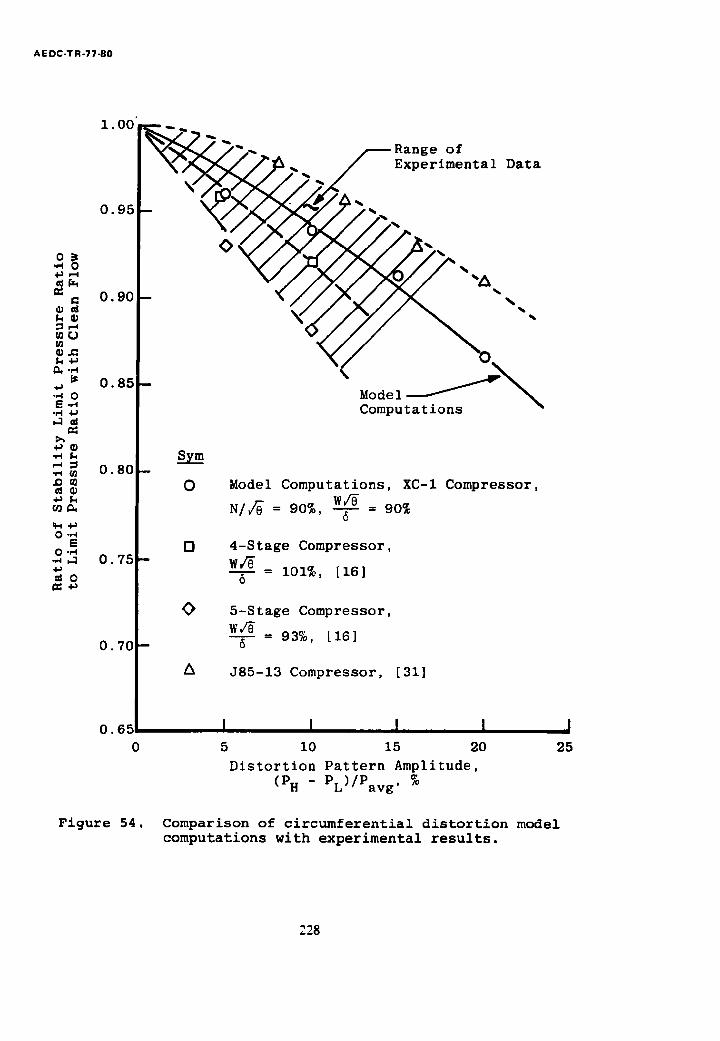
AE DC-T R-77-80
1. O0 ~ ~". - . y Range o f
~ ~ / ~ / ~ / / ' ~ ~ ~ E x p e r i m e n t a l D a t a
0.
85 / -- Model • ~ o ~ C o m p u t a t i o n s ,-3 ~1
.,-i
.O ~0 O
• ~ g., r n ~
O . , . d [] O . , ' d
O
0 . 8 0 --
O. 75 -
0 . 7 0 -
0 . 6 5
0
s_~
0
D
0
A
Model Computations, XC-I Compressor,
Wv~" = 90% N / ¢ ~ = 90%,
4 - S t a g e C o m p r e s s o r ,
= lO1%, [16] 6
5 - S t a g e Compressor,
w4~ 6 = 93%, [ 1 6 ]
J 8 5 - 1 3 C o m p r e s s o r , [31]
I I I I 5 i 0 15 20
Distortion Pattern Amplitude, (PH - P L ) / P a v g ' %
! 25
Figure 54, Comparison of circumferential distortion model computations with experimental results.
228
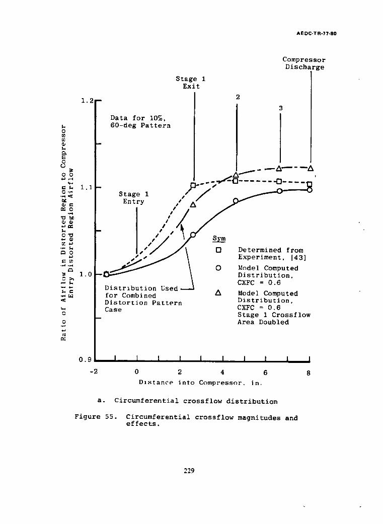
AEDC-TR-77-80
O
E o o o o
W-
re O
O~
o
Z~
0
0
1 . 2 -
1 .1
1 . 0
0 . 9
-2
D a t a f o r 10~, 6 0 - d e g P a t t e r n
Stage 1 Exit
2
C o m p r e s s o r D i s c b a r g e
o.-- t "I-o_ . . . . . . ~ . . . .
Stage 1 / / _ ~.....O"-'-'<2 Entry / Z~"
- I . . ) " Y , s _ ~
• 0 Determined from ~• / /\ 0 Determined • • S , s - / ~ Experiment, [43]
~ ~ \ O Model Computed D i s t r i b u t i o n , /
CXFC = O. 6 D i s t r i b u t i o n U s e d - - - J f o r Combined Zl Mode] Computed D i s t o r t i o n P a t t e r n D i s t r i b u t i o n , Case CXFC = 0 . 6
_ S t a g e 1 C r o s s f l o w Area D o u b l e d
i I I I l I I I I I
0 2 4 6 8
D i s t a n c e i n t o C o m p r e s s o r , i n .
a. Circumferential crossflow distribution
Figure 55. Circumferential crossflow magnitudes and effects.
229

AE DC-TR-77-80
0
0
E 0 U
4.0
3.5
3 . 0 m
m
m
2.5
31
o
s~ ~ /Stage i Crossflow
_" ~ t...oa ,~. " f " ° L Cr°ss fl°w---~ 2 , 1.0%
o • 1.4% ~ ~ •
O,
d,
N/J6 = 90%
Svm _.x..__
O
A
Crossflow. CXFC = 0.6, 10t, 60-deg Distortlon
Stage 1Crossflow Doubled, 10~. 60-deg Distortion
No Distortxon
I I I I I I 32 33 34
Corrected Airflow
b. Effect on stability limit
I I 1 35 36
Figure 55. (Continued).
230
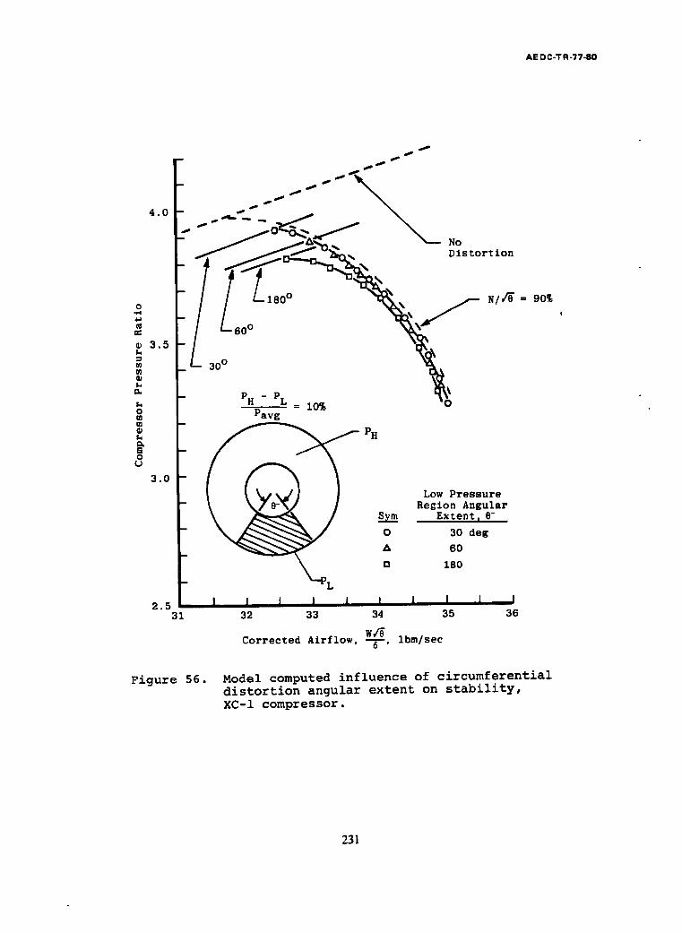
AE DC-TR-77-80
_ \ - ~ ~ ~ N _ _ No
180 °
~ 3 .5
~ L 3 ° ° " ~ - - PH - PL = I 0 % ~ i Pavg
3 . 0
2 . 5 ' - 31
o w o
[] o o
PH
O
D
L
Low P r e s s u r e Region Angu la r
Ex ten t~ 0-
30 deg
60
180
32 33 34 35 36
w,~ C o r r e c t e d A i r f l o w , --~--, lbm/sec
N / / ~ = 90~
Figure 56. Model computed influence of circumferential distortion angular extent on stability, XC-I compressor.
231
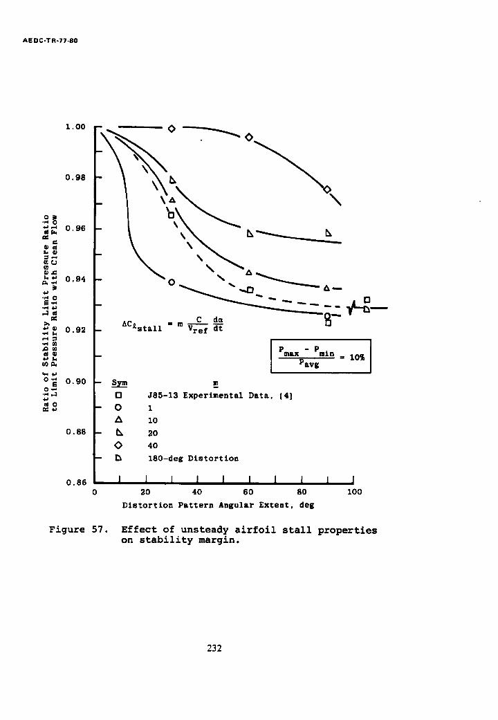
AE DC-T R-77-80
I O0
0 9 8
O R "~ O ~ 0 9 6
k ~ 0 9 4
°F,,I 0
~ 0 9 2
.,..i m
m ~
o F 0 9 0 o ~ • .4 ,.] 4~ ~ o
0.88
0.86
-
-- I Pmax - Pmln = 10~ [
I P a v g I - s _ ~ m_
O J85-13 E x p e r i m e n t a l D a t a , [ 4 ]
- O I
10
- h 20
O 40
- r~ 1 8 0 - d e e D i s t o r t i o n
i I I I I I I I I I 20 40 60 80 I00
D l s t o r t L o n P a t t e r n A n g u l a r E x t e n t , d e g
Figure 57. Effect of unsteady airfoil stall properties on stability margin.
232

A E DC -T R-7 7 -80
~..... ~ " " ~'*" ° " " ~ i0 Distortion 4.0 ....~
.~ . j , . . . ~ - - % o , , , , , / - - . , ~ -- , o~
= ~ o ~ - / ~ ~ -N-\o',
I"1 15%
- 0 2o~
M T H
8 9 . 7 % 89. 370
89.1%
88.9%
m
2.5 I i I I I I I I I I 31 32 33 34 35 36
Corrected Airflow, W/O Ibm/sec 6 '
Figure 58. Model computed influence of circumferential temperature distortion on stability, XC-I compressor.
233
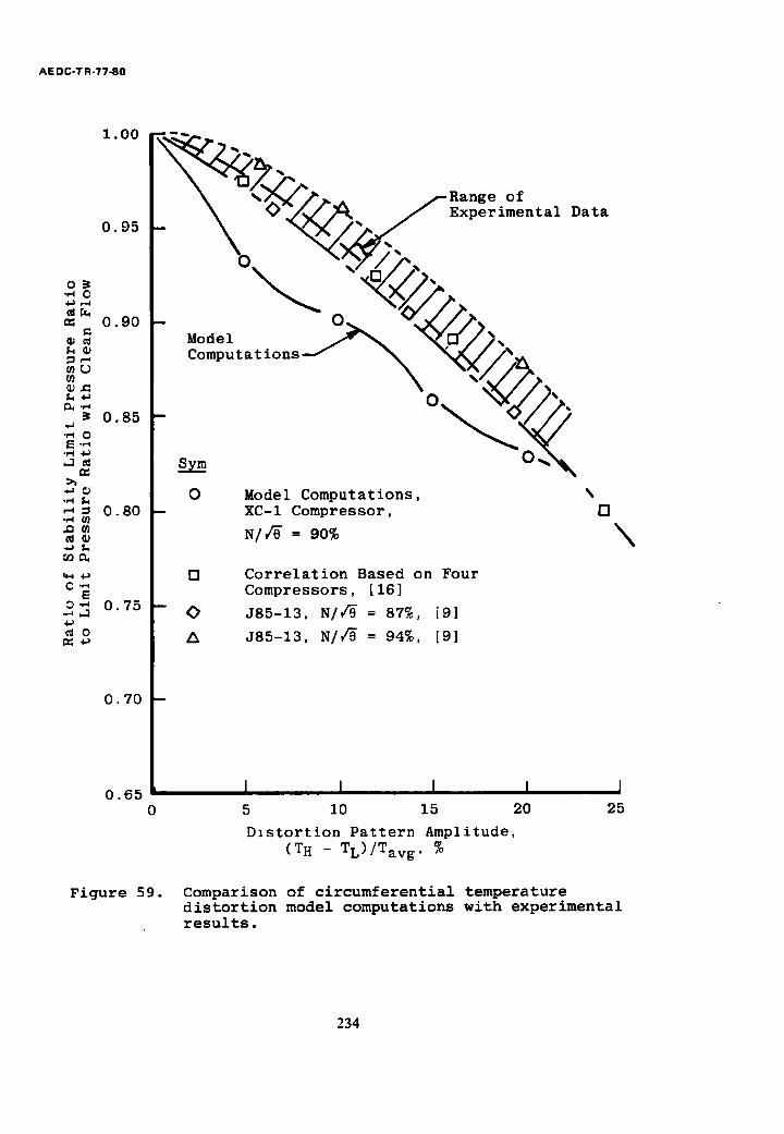
AE DC-T R-77-80
1.00
0 . 9 5
o 3 • ,~ O 4 J , - 4
0 . 9 0 -
~ . , ~
0.85 -- .J
• ~ O
~ 0.80 -
C'~ E
O -~ O. 75 --
¢d O
0 . 7 0 --
0 . 6 5 0
Figure 59.
Range o f E x p e r i m e n t a l D a t a
o M o d e l • C o m p u t a t i o n s
~ J
o M o d e l C o m p u t a t i o n s , XC-1 C o m p r e s s o r ,
N / ~ = 90%
[3
<>
C o r r e l a t i o n B a s e d o n F o u r C o m p r e s s o r s , [ 1 6 ]
J 8 5 - 1 3 , N/CrO = 87%, [9 ]
J 8 5 - 1 3 , N / / 9 = 94%, [ 9 ]
[]
I l I I I 5 10 15 20 25
D i s t o r t i o n P a t t e r n A m p l i t u d e , (T H - T L ) / T a v g , %
Comparison of circumferential temperature distortion model computations with experimental results.
\
234
AE DC-TR-77-80
APPENDIX B
COMPRESSOR DETAILS AND STAGE CHARACTERISTICS
Allison XC-I Compressor
Figure B-I (Appendix C) 1 shows the overall com-
pressor map for the Allison XC-I lift engine, four-stage
compressor. Key dimensions and design performance are given
in Table B-I (Appendix C). 1 Stage characteristics used in !
the model are given in Figs. B-2a through B-2d. The mean of
the outer and inner radii was used in the stage flow and
pressure coefficient calculations. All the information was
taken from [43]. Dimensions and data not tabulated in the
report were obtained from scaling drawings and figures.
NACA-8 Compressor
Figure B-3 gives the overall performance of the
NACA eight-stage research compressor. Principal dimensions
and design performance are given in Table B-2. Stage
characteristics are given in Figs. B-4a through B-4h. Mean
radii were used in the flow coefficient, equivalent pressure,
and equivalent temperature ratio computations. All infor-
mation on the NACA-8 compressor was taken from [44, 45, 46].
IAII figures and tables for Appendix B appear in Appendix C.
235
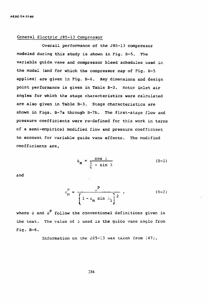
AE DC-TR-77-80
General Electric J85-13 Compressor
Overall performance of the J85-13 compressor
modeled during this study is shown in Fig. B-5. The
variable guide vane and compressor bleed schedules used in
the model (and for which the compressor map of Fig. B-5
applies) are given in Fig. B-6. Key dimensions and design
point performance is given in Table B-3. Rotor inlet air
angles for which the stage characteristics were calculated
are also given in Table B-3. Stage characteristics are
shown in Figs. B-7a through B-7h. The first-stage flow and
pressure coefficients were re-defined for this work in terms
of a semi-empirical modified flow and pressure coefficient
to account for variable guide vane effects. The modified
coefficients are,
and
cos Sm= 1 (B-l)
--- sin 3
P r ) l,i
= , (B-2)
3 2 4m [ 1 - ~m sin "i]
where ¢ and ~P follow the conventional definitions given in
the text. The value of 3 used is the guide vane angle from
Fig. B-6.
Information on ~he J~5-13 was taken from [47].
236

AE DC-TR-77-80
APPENDIX C
FIGURES AND TABLES FOR APPENDIX B
237
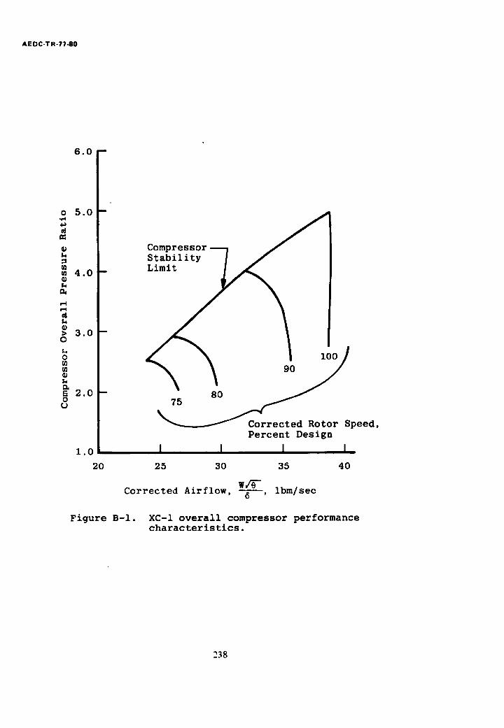
6.0
Compressor S t a b i l i t y Limit
o 5.0--
==
4 . 0 - -
r.4 p4
0 > 3 . 0 - - o
r,,., o
E 2.0-- o
1.0
20
AE DC-T R-77-80
5 90 100
C o r r e c t e d R o t o r S p e e d , P e r c e n t D e s i g n
I I I I 25 30 35 40
we~- Corrected Airflow, 6 , Ibm/sec
Figure B-I. XC-I overall compressor performance characteristics.
238
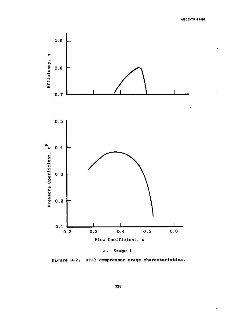
AE DC-TR-77-80
0 . 9 ~
~J
® 0.8 I °~1
q-I q~
0 . 7
0 . 5
0 . 4 --
~ 0 . 3 - -
0
i,t
• 0 . 2 - N
0 . 1 0 . 2
I I I I 0.3 0.4 0.5 0.6
Flow Coefficient,
a. Stage 1
Figure B-2. XC-I compressor stage characteristics.
239
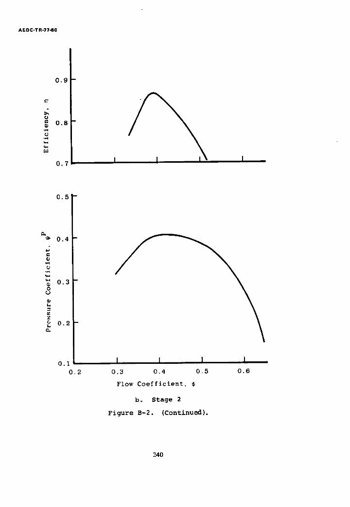
A E D C - T R - 7 7 - 8 0
0 . 8 .,=1
0 , 9
0 . 7 I I I I
0 . 5
0 . 4
4~
k~ m ¢ 0 . 3 O
b.i
0 . 2 - L. e'
0 . 1 0 . 2
l I I 0.3 0.4 0.5
Flow Coefficient, ¢.
b. Stage 2
Figure B-2. (Continued).
I
0.6
240
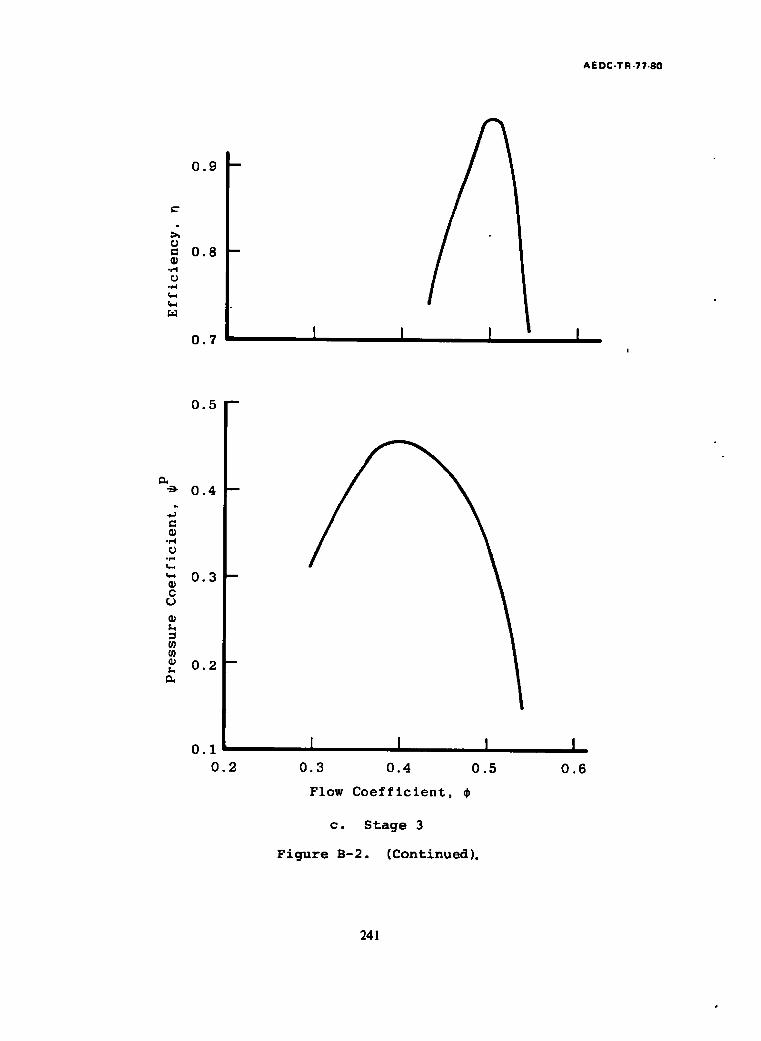
AE DC-TR-77-80
0 . 9
C"
0 . 8 (D
- 4 %.4
0 . 7 I I
0 . 5
0.4
-4
°~
0.3 --
C
¢ 0 2 - -
0 . 1
0 . 2
I I I 0.3 0.4 0.5
Flow Coefficient,
c. Stage 3
Figure B-2. (Continued).
I 0 . 6
241
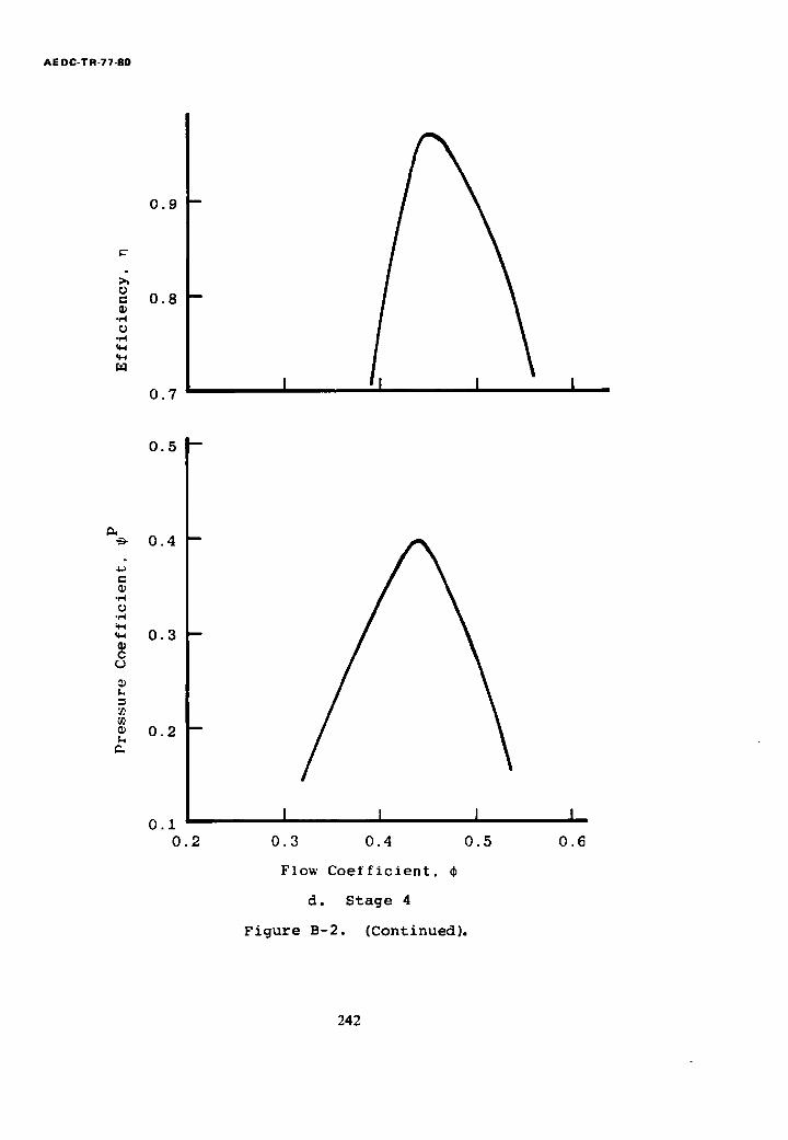
AE 0C-TR-77-80
0.9
0.7
= 0.8
-,d
-,d
0.5
0.1 0.2
0.4 --
4J
0 .rd b.4
0.3 -- OJ C 0
k
• 0.2 -- C.
I I i 0.3 0.4 0.5
Flow Coefficient, ¢
d. Stage 4
Figure B-2. (Continued).
I 0 . 6
242
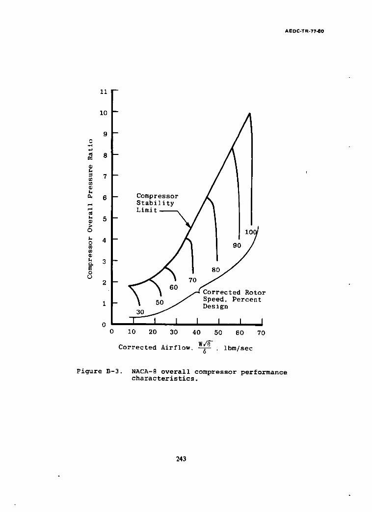
AEDC-T R-77-80
ii
i0
9
= 7
~ 6
~ 5
~ 4
~ 3
2
1
0
C o r r e c t e d A i r f l o w .
!
!ii!!- o ~o ~o~°
I i0 20 30 40 50 60 70
w/E~ 6 , Ibm/sec
Figure B-3. NACA-8 overall compressor performance characteristics.
243
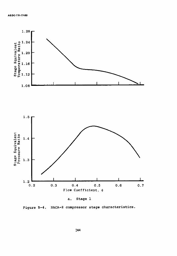
AE DC-T R-77-80
1 . 2 8 -
~ . ~ 1 . 2 4 -
~ n e i. 20 -
~ m 1.16 -
eE 4~ m ~ 1 . 1 2 -
1.08 ] l
1.5
o
~ 1.4 m
m z ~k ,.u m
~o ~ 1.3
1.2 I I i i I 0.2 0.3 0.4 0.5 0.6 0.7
Flow Coefficient, ¢
a. Stage 1
Figure B-4. NACA-8 compressor stage characteristics.
244
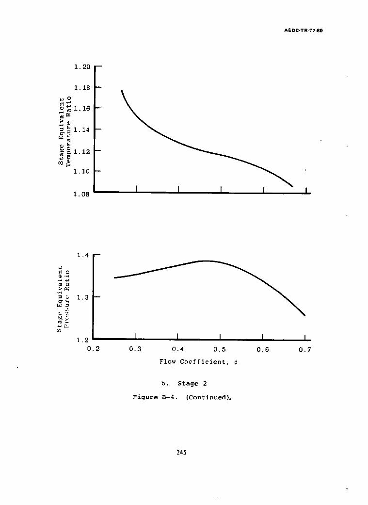
1 . 2 0
1.18
1.08
O
~ 1 . 1 6
g ~ 1 .14
E
1 . 1 0
I I I [
AE DC-TR-77-80
.Ill m
>he
& ~ Z
~ 2 . . .
1 . 4
1 . 3
1 . 2
0 . 2
I I I I I 0 . 3 0 . 4 0 . 5 0 . 6 0 . 7
F low Coefficient, ¢
b. Stage 2
Figure B-4. (Continued).
245
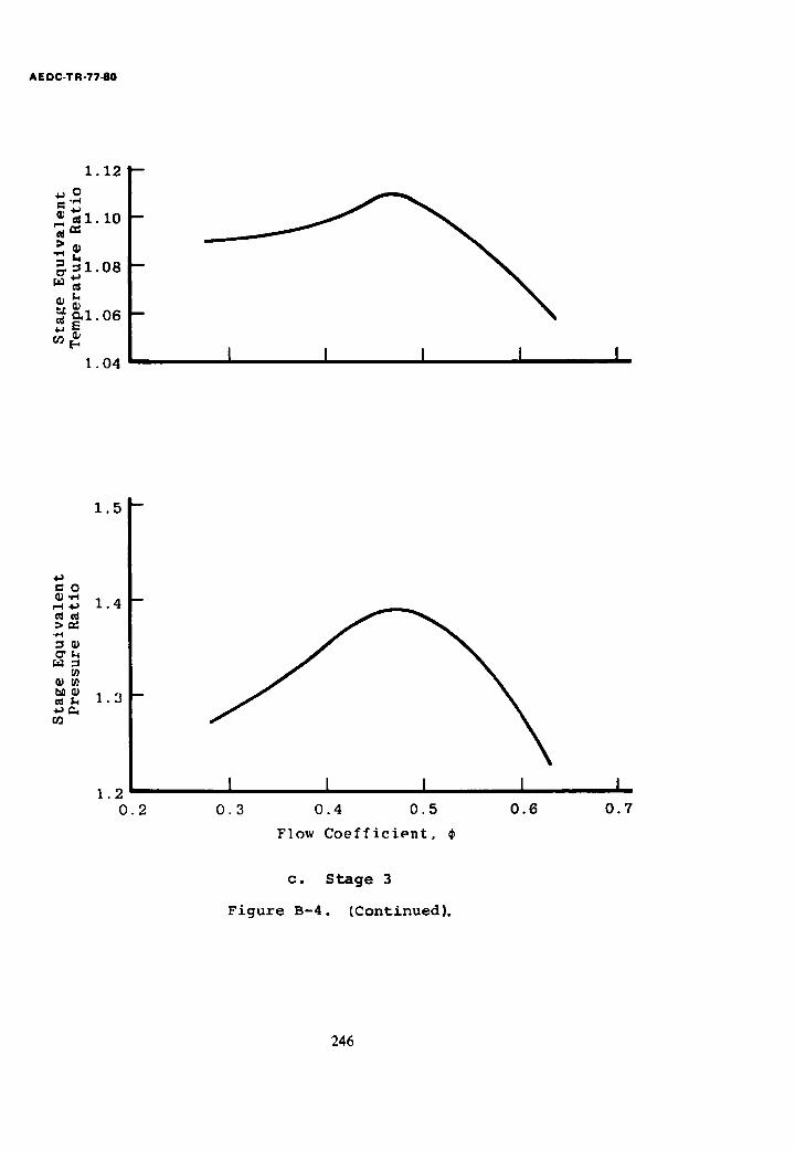
A E OC -T R -77-80
1.12
~I. i0
=~1 08
~1 06 ~E " m[..,
I . 04 I I I I I
~ 0 ~.~
.4
1 .5
1 .4
1 , 3 m
1.2 0 . 2
I I I I 0 . 3 0 . 4 0 . 5 0 . 6
F l o w C o e f f i c i e n t ,
I 0.7
c. Stage 3
Figure B-4. (Continued).
246

AE DC-T R-77-80
O
4J
~E
I. 12
i. I0
1.08
1.06 I I I I
+~
O
cO
1.5
1.4
1.3
1.2 0.3
I I I 0.4 0.5 0.6
Flow Coefficient,
d. Stage 4
Figure B-4. (Continued).
I 0 . 7
¢
247
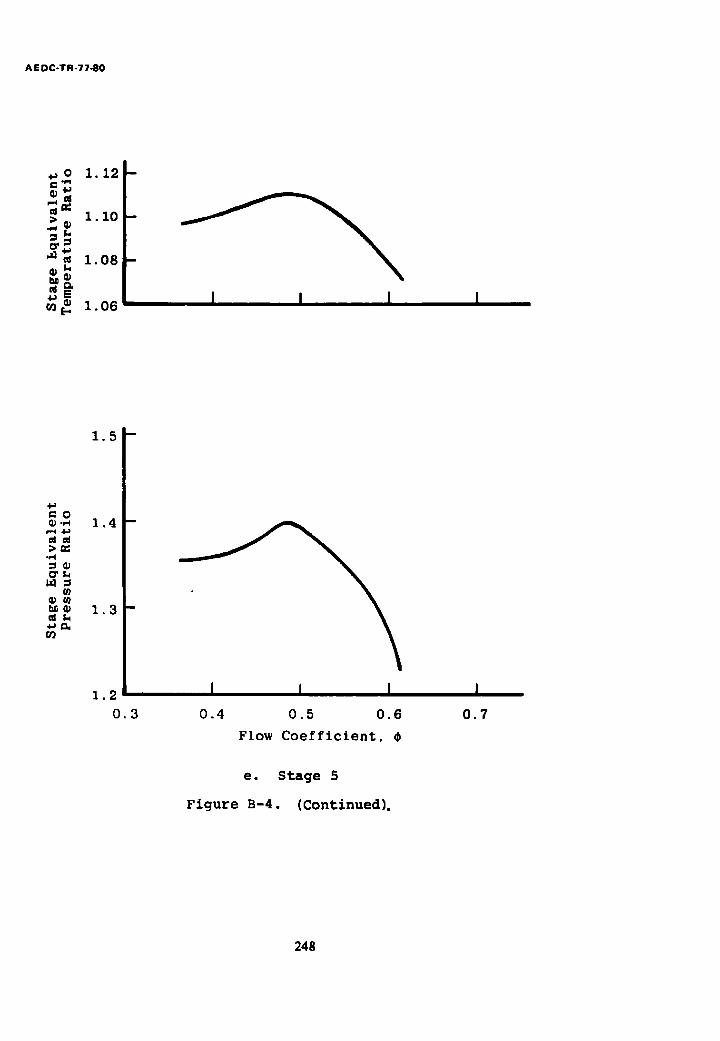
AEDC-TR-77-80
wo 1.12
~ 1 . 1 o
, a ~ 1 . 0 8 g~ , oE rn~, 1 .06
=0
e=q ,~
M
5'}
1.5
1.4
1.3 --
1.2
0.3
I I I 0 . 4 0 . 5 0 . 6
Flow C o e f f i c i e n t , ¢
I 0.7
e. Stage 5
Figure B-4. (Continued).
248

AEDC-TR-77-80
~o 1.12
1.10
1.08
1.06 r i I I
=0
cr~
1.5
1.4
1.3
I
1.2
0.3
I J I
0 . 4 0 . 5 0 . 6
Flow C o e f f i c i e n t ,
I
0.7
f. Stage 6
Figure B-4. (Continued).
249

AEDC-T R-77-80
~o 1.10
r-4
~ 1.08
~ • 1.06
m ~ 1.04
4~
= 0 ~J.~
"4
1.4
1.3
1.2
1.1
1.0 0.4 0 .5 0 .6 0 . 7
Flow C o e f f i c i e n t .
I
0.8
g. Stage 7
Figure B-4. (Continued).
250
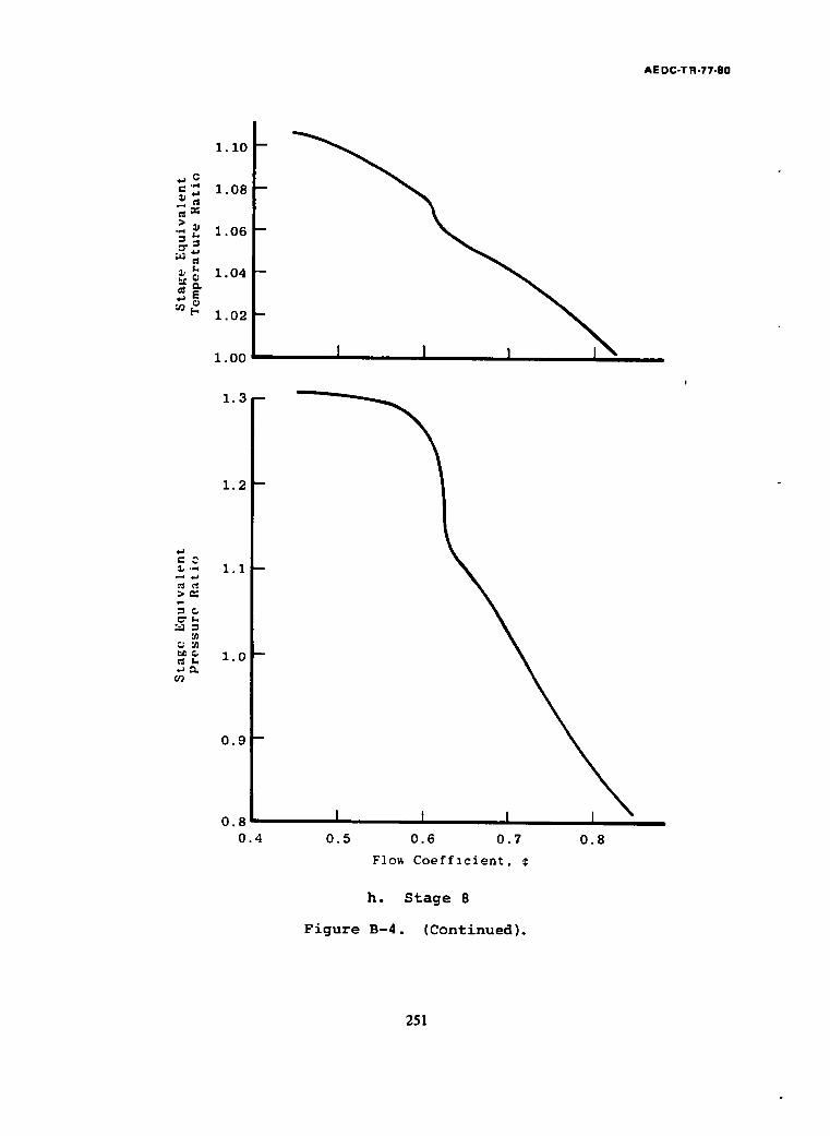
AE DC-TR-77-80
i. I0
~J
1 . 0 8
1 . 0 6
1.04
1.02
1.00
1.3
1 . 2
1 , 1 m
1 . 0 - -
0 . 9 --
0 . 8
0 . 4
I 0 . 5
~C
I 0 . 6 0 . 7 0 . 8
Flow C o e f f i c i e n t , ¢
h. Stage 8
Figure B-4. (Continued).
251

t~ t~
8
~:'0~ 7 ~ 0 / Experimental
o 5 ~ / ! or
8 4
• 8
325 30 35 40 45
W~rO Ibm/sec Corrected Airflow, ~ ,
m
? -4
& O
Figure B-5. J85-13 overall compressor performance characteristics.
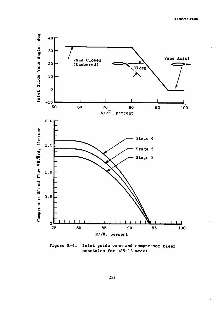
A EDC-TR-77-80
40 - ' 0
d "~ 30 -
e~
¢ 2 0 - - ¢1
1O-
F-4
-10 50
2 . 0
o
" 1 . 5
1.0 -
0.5
° I (¢/ -
I~ -
E 0 -
0 • 7 5
Vane Axial
I I I I I, 60 70 80 90 100
N/~-, percent
S t a g e 4
S t a g e 5
S t a g e 3
80 85 90 95
N/VrS, pe rcen t
100
Figure B-6. Inlet guide vane and compressor bleed
schedules for J85-13 model.
253

0 . 9 0
0.85
0
.,.4 ~J
"~ 0 8 0 ~ •
0.73
0.3
~%~ 0 .2
e -
°r,d
~.~ ~ , . ~ 0 . 1
0
AE DC-T R-77-80
l I I I F l o w C o e f f i c i e n t ,
0.3 0.4 0.5 0.6
Modified Flow Coefficient, Cm
a. Stage 1
Figure B-7.
0.7
J85-13 compressor stage characteristics.
254
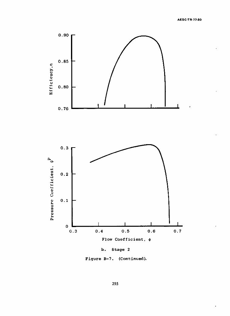
0 . 9 0
0.85
=
w~ ,~ O. 8 0
O. 76 I I
AEDC-TR-77-80
4a
-F4
0.3
0.2
0.1
0.3
I I I 0.4 0.5 0.6
Flow Coefficient,
b. Stage 2
Figure B-7. (Continued).
I 0.7
255
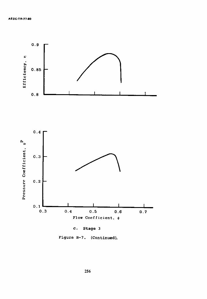
AE DC-TR-77-80
0.9
= 0.85
0 . 8 I I I I
C~
°~
-I
O~
0 . 4
0 . 3
0 . 2 m
O . 1 0 . 3
I I I 0 . 4 0 . 5 0 . 6
F l o w C o e f f i c i e n t . ¢
I 0.7
c. Stage 3
Figure B-7. (Continued).
256

AE 0C-TR-77-80
0 . 9 0 -
" 0 . 8 5 -
O. 8 0 I I I I
-r4
O
O
0.3
0.2
0.1
0 0.3
I I I 0 . 4 0 . 5 0 . 6
F l o w C o e f f i c i e n t .
I 0.7
d. Stage 4
Figure B-7. (Continued).
257
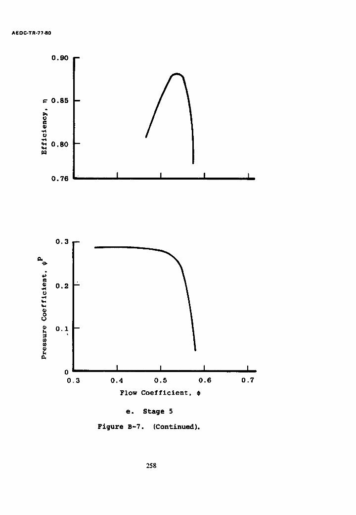
AEDC-TR-77-80
O. 9 0 -
= 0.85
£ 0
0
~ 0 . 8 0
0.76 I I i I
0.3
4~
0 . 2 ";" .t4
0
0.1 --
0 0.3
I I I 0.4 0.5 0.6
Flow Coefficient,
I 0.7
e. Stage 5
Figure B-7. (Continued).
258
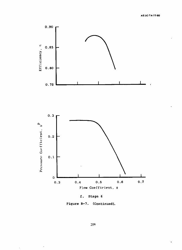
0 . 9 0 --
0.85
%.
0.80
0.76
0 , 3 m
AE DC-TR-77-80
l i l l
q. , e .
. , .q ° .
o,..4
L .
Y .
L ' L_
e ~
0 . 2 m
0 . I - -
0
0 . 3
I 0 . 4
l I 0 . 5 0 . 6
F l o w C o e f f i c i e n t ,
l 0.7
f. Stage 6
Figure B-7. (Continued).
259
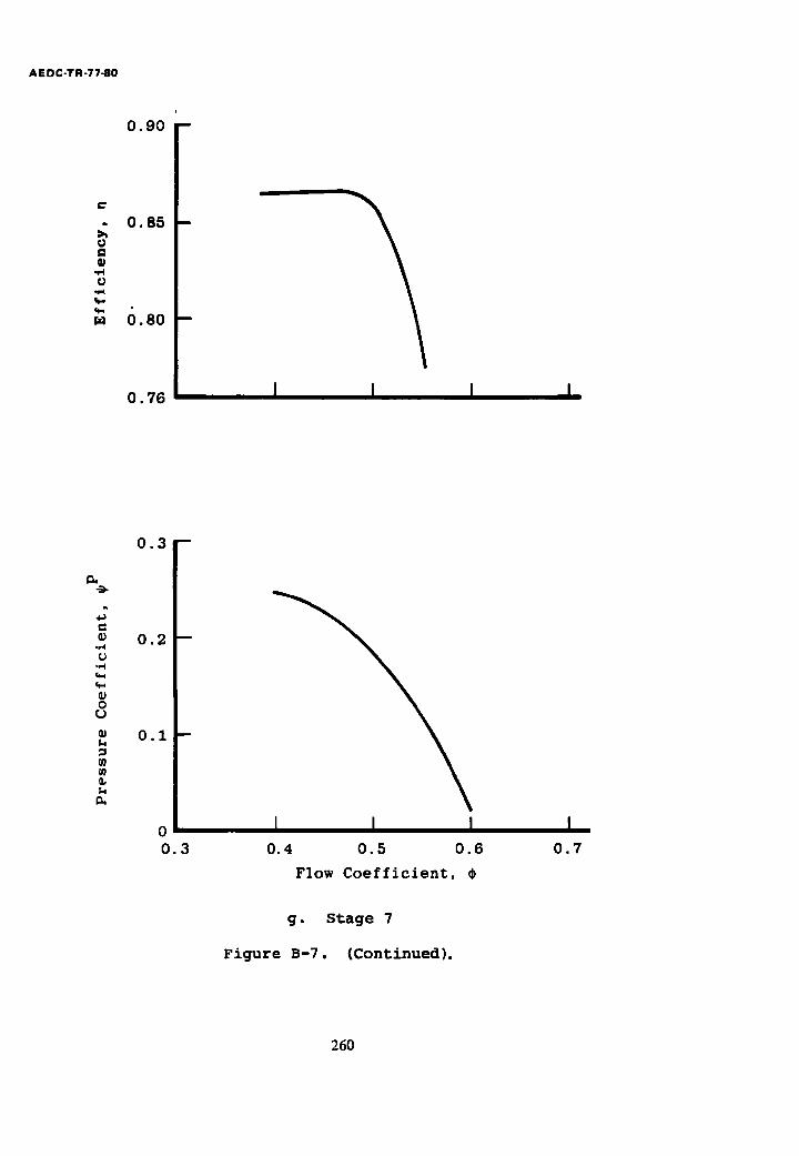
AEDC-TR-77-80
0 . 9 0
O. 85
0.80
0 . 7 6 I I I I
.--D-
.-4 U
0
0 . 3
0 . 2
0 . i
0 0 . 3
i I I 0 . 4 0 . 5 0 . 6
F l o w C o e f f i c i e n t , ¢
l 0.7
g. Stage 7
Figure B-7. (Continued).
260
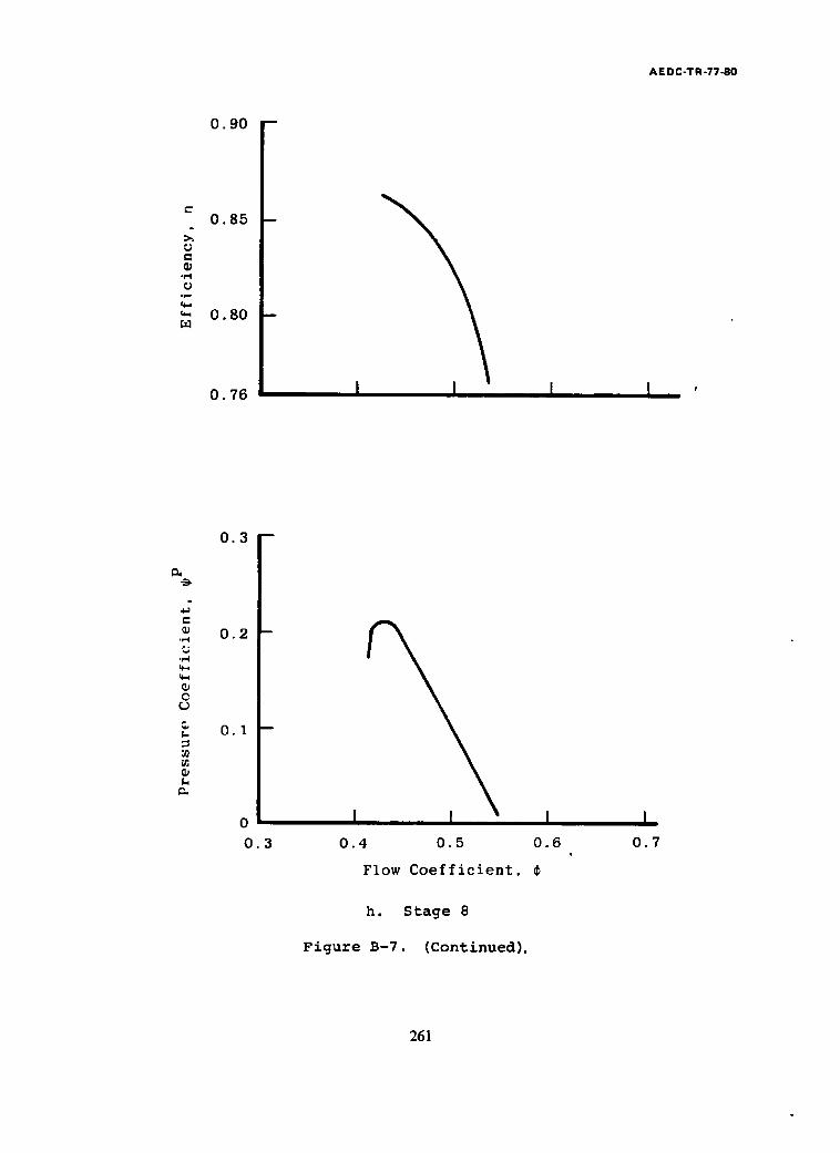
O. 90
0 . 8 5
~J e~
.=4 0
;2 ~ O. 8 0
O. 7 6
0 . 3
I I
9 -
p,
.-I
O
k
0 . 2
O . 1 B
0
0 . 3
I I
A E D C - T R - 7 7 - 8 0
I 0 . 6 0 . 4 0 . 5
Flow C o e f f i c i e n t ,
I 0.7
h. Stage 8
Figure B-7. (Continued).
261
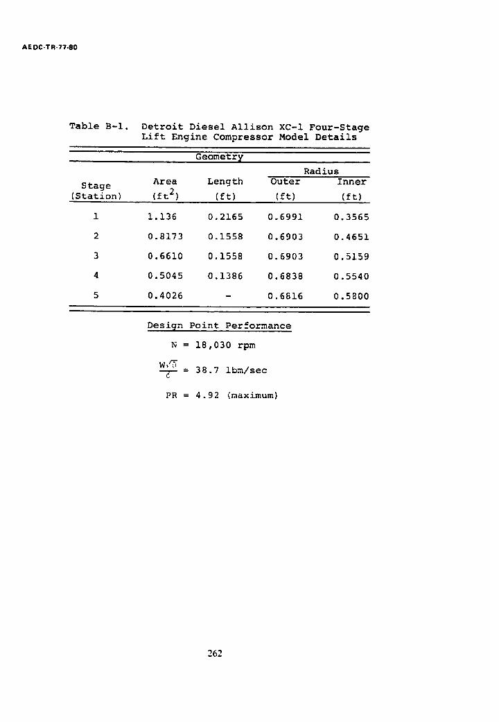
AE DC-TR-77-80
Table B-I. Detroit Diesel Allison XC-I Four-Stage Lift Engine Compressor Model Details
Geometr[
Stage Area Length Outer
(Station) (ft 2) (ft) (ft)
Radius Inner
(ft)
1 1.136 0.2165 0.6991 0.3565
2 0.8173 0.1558 0.6903 0.4651
3 0.6610 0.1558 0.6903 0.5159
4 0.5045 0.1386 0.6838 0.5540
5 0.4026 - 0.6816 0.5800
Design Point Performance
N = 18,030 rpm
W~'{i = 38.7 ibm/sec
6
PR = 4.92 (maximum)
262
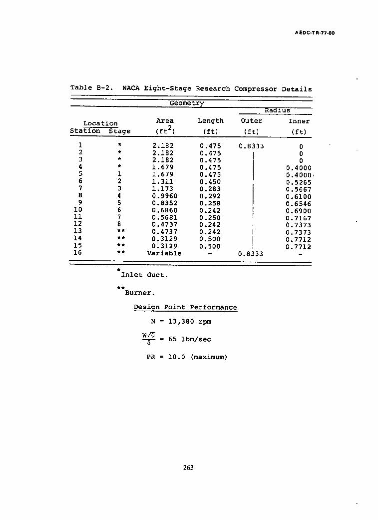
A EDC-T R-77-80
Table B-2. NACA Eight-Stage Research Compressor Details
Geometry
Location Area Length Outer Inner
Station Stage (ft 2) (ft) (ft) (ft)
1 * 2.182 2 * 2.182 3 * 2.182 4 * 1.679 5 1 1.679 6 2 1.311 7 3 1.173 8 4 0.9960 9 5 0.8352
10 6 0.6860 ii 7 0.5681 12 8 0.4737 13 ** 0.4737 14 ** 0.3129 15 ** 0.3129 16 ** Variable
0.475 0.475 0.475 0.475 0.475 0.450 0.283 0.292 0.258 0.242 0.250 0.242 0.242 0.500 0.500
0.8333
0.8333
0 0 0
0.4000 0.4000, 0.5265 0.5667 0.6100 0.6546 0.6900 0.7167 0.7373 0.7373 0.7712 0.7712
Inlet duct.
Burner.
Design Point Performance
N = 13,380 rpm
- 65 ibm/sec
PR = I0.0 (maximum)
263

AE DC-TR-77-80
Table B-3. General Electric J85-13 Eight-Stage Compressor Details
Location
Station Stage
Geometry Radius
Area Length Outer Inner
(ft 2) (ft) (ft) (ft)
Rotor Inlet
Air Angle (deg)
1 *
2 * 3 * 4 * 5 1 6 2 7 3 8 4 9 5
10 6 11 7 12 8 13 ** 14 ** 15 ** 16 **
1.300 0.1856 1.300 0.1856 1.300 0.1856
1.150 0.1856 1.066 0.1856 0.8395 0.1364 0.6821 0.1116 0.5630 0.09767 0.4690 0.08725 0.4055 0.07892 0.3698 0.07750 0.3580 0.09883 0.3542 0.i000 1.312 0.i000 0.3542 0.1000
Variable
0.6708 0.6708 0.6708 0.6708 0.6458
0.6458
0 1900 0 1900 0 1900 0 2812 0 3156 0 3935 0 4472 0 4878 05175 0.5367 0.5472 0.5506 0.5506 0.2683 0.5506
0 0 0 0
Scheduled 5.4
12.1 14.8 19.4 23.2 22.2 21.6
0 0 0 0
Inlet duct.
Burner.
Design Point Performance
N = 16,500 rpm
w/6 - 43 lbm/sec
PR = 7.7 (maximum)
264

AE DC.TR-77-80
A
ACC
ACR
ARR
ARZ
AZ
a
C
C d
C£
CF (r)
C P
C V
CXFC
CXFR
D
DLR
EPR
NOMENCLATURE
Area
Projected area of control volume circumferential
surface in the circumferential direction
Projected area of control volume circumferential
surface in the radial direction
Projected area of control volume radially-facing
surface in the radial direction !
Projected area of control volume radially-facing
surface in the axial direction
Control volume area normal to axial direction
Acoustic velocity; blade spacing; a constant
Blade chord length
Blade drag coefficient
Blade lift coefficient
Stage characteristic correction factor for
radial variation
Specific heat at constant pressure
Specific heat at constant volume
Circumferential crossflow coefficient
Radial crossflow coefficient
Blade drag force
Dynamic lift amplitude ratioed to quasi-steady-
state lift
Stage equivalent pressure ratio, Eq. (47)
265
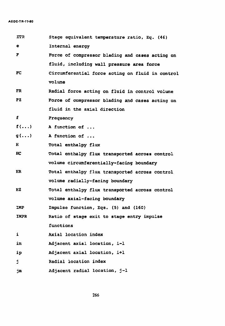
AE DC-T R-77-80
ETR
e
F
FC
FR
FZ
f
f(...)
g(...)
H
HC
HR
HZ
IMP
IMPR
i
im
ip
J
jm
Stage equivalent temperature ratio, Eq. (46)
Internal energy
Force of compressor blading and cases acting on
fluid, including wall pressure area force
Circumferential force acting on fluid in control
volume
Radial force acting on fluid in control volume
Force of compressor blading and cases acting on
fluid in the axial direction
Frequency
A function of ...
A function of ...
Total enthalpy flux
Total enthalpy flux transported across control
volume circumferentially-facing boundary
Total enthalpy flux transported across control
volume radially-facing boundary
Total enthalpy flux transported across control
volume axial-facing boundary
Impulse function, Eqs. (5) and (160)
Ratio of stage exit to stage entry impulse
functions
Axial location index
Adjacent axial location, i-1
Adjacent axial location, i+l
Radial location index
Adjacent radial location, j-i
266
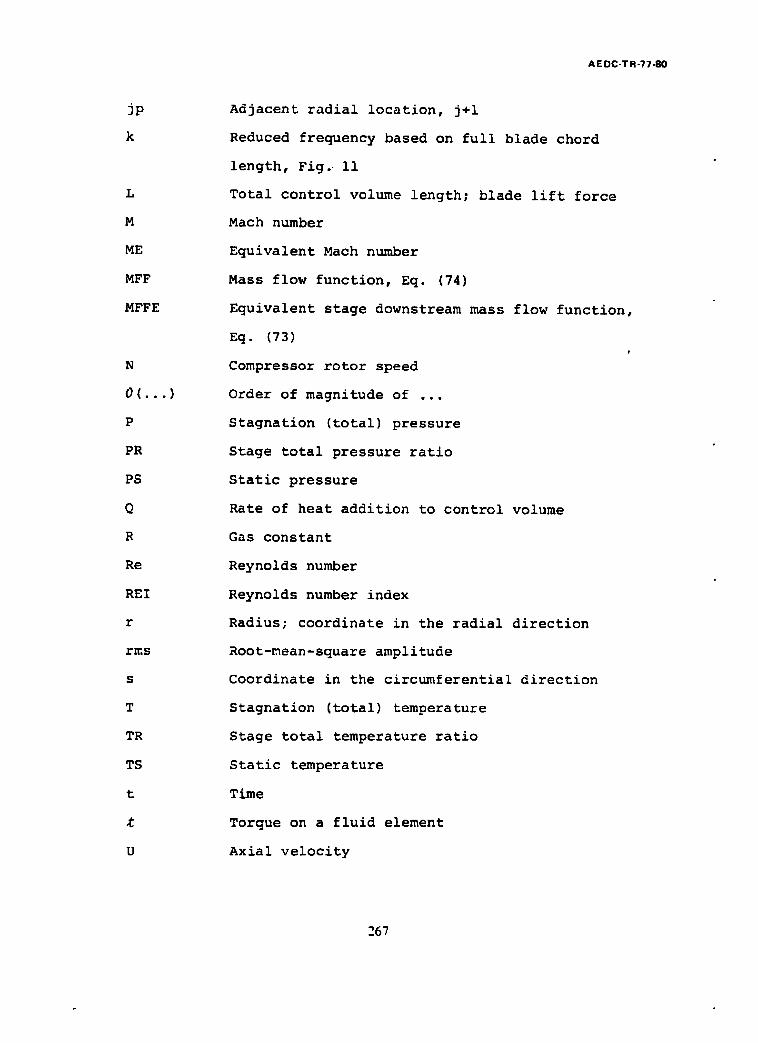
JP
k
L
M
ME
MFF
MFFE
N
0 ( . . . )
P
PR
PS
Q
R
Re
REI
r
r ~ s
s
T
TR
TS
t
t
U
AE DC-T R-77-80
Adjacent radial location, j+l
Reduced frequency based on full blade chord
length, Fig. ii
Total control volume length; blade lift force
Mach number
Equivalent Mach number
Mass flow function, Eq. (74)
Equivalent stage downstream mass flow function,
Eq. (73) f
Compressor rotor speed
Order of magnitude of ...
Stagnation (total) pressure
Stage total pressure ratio
Static pressure
Rate of heat addition to control volume
Gas constant
Reynolds number
Reynolds number index
Radius; coordinate in the radial direction
Root-mean-square amplitude
Coordinate in the circumferential direction
Stagnation (total) temperature
Stage total temperature ratio
Static temperature
Time
Torque on a fluid element
Axial velocity
267
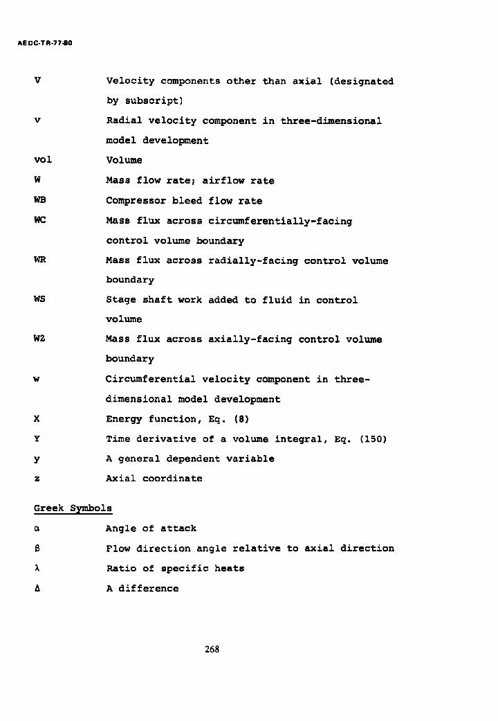
AE DC-TR-77-80
V
V
vol
W
WB
WC
WR
WS
WZ
W
X
Y
Y
Z
Velocity components other than axial (designated
by subscript)
Radial velocity component in three-dimensional
model development
Volume
Mass flow rate; airflow rate
Compressor bleed flow rate
Mass flux across circumferentially-facing
control volume boundary
Mass flux across radially-facing control volume
boundary
Stage shaft work added to fluid in control
volume
Mass flux across axially-facing control volume
boundary
Circumferential velocity component in three-
dimensional model development
Energy function, Eq. (8)
Time derivative of a volume integral, Eq. (150)
A general dependent variable
Axial coordinate
Greek S~mbols
B
A
Angle of attack
Flow direction angle relative to axial direction
Ratio of specific heats
A difference
268
AE DC-TR-77-80
Ap
6
£
had
e
m
8
P
~P ~T
Pressure fluctuation amplitude
Ratio of compressor entry total pressure to
standard day, sea-level-static pressure
A constant; an error magnitude
Stage adiabatic efficiency
Angular location; ratio of compressor inlet
total temperature to standard day, sea-level-
static temperature
Angular extent of low pressure region in r
circumferential distortion pattern
Blade chord-to-axial direction angle or stagger
angle
Density
Stage pressure coefficient
Stage temperature coefficient (stage loading
parameter)
Angular rotor speed; circular frequency
Superscripts
Average or effective value
P Pertaining to pressure
T Pertaining to temperature
Subscripts
0,1,2,...
ad
avg
crit
Location or station designators
Adiabatic
Average value
Critical value
269
AE DC-T R-77-80
dyn
exit
H
i
im
ip
ijk
J
jm
Jp
k
km
kp
L
l o c
m
m a x
m i n
n
P
radial avg
ref
rel
Dynamic value
Pertaining to control volume exit plane
High
Axial location index
Adjacent axial location, i-I
Adjacent axial location, i÷1
Three-dimensional location index, refers to
value at location i, j, k
Radial location index
Adjacent radial location, j-1
Adjacent radial location, j+l
Circumferential location index
Adjacent circumferential location, k-1
Adjacent circumferential location, k+l
Low
Local value
Modified form; minus one
Maximum value
Minimum value
Last location, e.g., in, last axial location
in control volume
Plus one
Average value along a radius, average at
constant 8
Reference value
Relative value, usually relative to rotor
blade motion
270
AEOC-TR-77-80
ring avg
stall
SS
SW
wh
Z
Average value along a circle, average at
constant r
Value at stall
Steady-state value
Swirl
Wheel
Axial component
271